spread option pricing using adi methods · spread option pricing using adi methods vida...
TRANSCRIPT
1
Spread option pricing using ADI methods
Vida Heidarpour-Dehkordi and Christina C. Christara1
Department of Computer Science
University of Toronto
Toronto, Ontario M5S 3G4, Canada
{vidahd,ccc}@cs.toronto.edu
Abstract
Spread option contracts are becoming increasingly important, as they frequently arise in the energy
derivative markets, e.g. exchange electricity for oil. In this paper, we study the pricing of European
and American spread options. We consider the two-dimensional Black-Scholes Partial Differential
Equation (PDE), use finite difference discretization in space and consider Crank-Nicolson (CN) and
Modified Craig-Sneyd (MCS) Alternating Direction Implicit (ADI) methods for timestepping. In or-
der to handle the early exercise feature arising in American options, we employ the discrete penalty
iteration method, introduced and studied in Forsyth and Vetzal (2002), for one-dimensional PDEs dis-
cretized in time by the CN method. The main novelty of our work is the incorporation of the ADI
method into the discrete penalty iteration method, in a highly efficient way, so that it can be used for
two or higher-dimensional problems. The results from spread option pricing are compared with those
obtained from the closed-form approximation formulae of Kirk (1995), Venkatramanan and Alexander
(2011), Monte Carlo simulations, and the Brennan-Schwartz ADI Douglas-Rachford method, as im-
plemented in MATLAB. In all spread option test cases we considered, including American ones, our
ADI-MCS method, implemented on appropriate non-uniform grids, gives more accurate prices and
Greeks than the MATLAB ADI method.
Keywords: Modified Craig-Sneyd, Alternating Direction Implicit method, two-dimensional Black-
Scholes, American option, spread option, exchange option, analytical approximation, numerical PDE
solution, penalty iteration 2
1 Introduction
Spread options are popular financial contracts for which, except the simplest case called exchange
contracts (i.e. strike = 0), there exist no analytical solutions. We are interested in pricing spread options,
using a numerical Partial Differential Equation (PDE) approach.
A spread option is a two-asset derivative, whose payoff depends on the difference between the prices
s1(t) and s2(t) of the two assets. Essentially, the European call (put) spread option gives the holder the
right, but not the obligation, to buy (sell) the spread s1(T ) − s2(T ) at the exercise price K, at maturity
time T .
In the energy markets, an example of a spread option is an option on the spark spread, which is the
difference between the price received by a generator for electricity produced and the cost of the natural gas
needed to produce that electricity. Another example of a spread option is an option on the crack spread,
which is the difference between the price of refined petroleum products and crude oil.
Several spread option pricing approaches can be used, such as Monte Carlo (MC) simulations or tree
(lattice) methods, however, for problems in low dimensions, the PDE approach is a popular choice, due to
1This work was supported by the Natural Sciences and Engineering Research Council of Canada2AMS: 65M06, 91G60.
July 4, 2017
2
its efficiency and global character. In addition, the essential parameters for risk-management and hedging
of financial derivatives, such as delta and gamma, are generally much easier to compute via the PDE
approach than via other methods.
We consider the basic two-dimensional Black-Scholes (BS) PDE and compute a numerical approxima-
tion to the solution using second-order finite differences (FD) discretization in space and Crank-Nicolson
(CN) or Alternating Direction Implicit (ADI) methods, more specifically, the Modified Craig-Sneyd
(MCS) method, for timestepping. Note that MCS is stable without stepsize restrictions, and exhibits
second-order convergence in both space and time when applied to PDEs with mixed derivative terms
([12], [13], [24]). To price American spread options a non-linear penalty term is added to the PDE, and
an iterative method is employed to solve the resulting problem. This technique is introduced in [8] for
one-dimensional problems and CN timestepping. Our focus in this paper is to incorporate the ADI-MCS
method efficiently into the penalty iteration. We present results from our ADI-MCS method on various
types of spread options and compare them to results from other PDE approximation methods, analytical
approximation formulae and MC simulation methods.
Regarding analytical formulae, for the case of European exchange options, there exists the Margrabe
formula [17], which gives the exact price of the exchange option, and is an accurate reference value
for comparison. For general European spread options, there is no formula that gives the exact price.
However, there exist analytical formulae that approximate the price of European spread options. These
approximations include Kirk’s formula [15] and the formula developed by Venkatramanan and Alexan-
der [22]. Kirk’s formula provides a good approximation of spread option prices when the strike K is small
compared to the current value of s2. Venkatramanan and Alexander [22] express the price of a European
spread option as the sum of the prices of two compound exchange options (CEOs), one to exchange vanilla
call options and the other to exchange vanilla put options. Using a conditional relationship between the
strike of vanilla options and the implied correlation, the authors reduce the problem to one-dimensional
put and call vanilla option computations.
For both European and American spread option test cases, we also consider two different numeri-
cal approximations in MATLAB. One is MATLAB’s implementation of the Douglas-Rachford (DR) ADI
timestepping (func. spreadsensbyfd), and another is the MC simulations (func. spreadsensbyls).
In the MATLAB function spreadsensbyfd, for American spread options, the ADI-DR timestepping
is combined with the Brennan-Schwartz algorithm [1], in order to solve the Linear Complementarity
Problem (LCP) arising when pricing American type options. In [10], the algorithm is re-formulated using
a form of LU decomposition, and this form is used in the MATLAB code.
Moreover, we display results of Greeks computed using our method, as well as MATLAB’s functions
spreadsensbyfd and spreadsensbyls. Finally, we present results for the free boundary.
In Section 2, we present the PDE along with initial and boundary conditions. The discretization of
the problem along the space dimension and the ADI time-stepping technique are described in Section
3. In Section 4, the handling of American options using the discrete penalty iteration method for both
CN and ADI timestepping is demonstrated. Special attention is paid in efficiently incorporating the ADI-
MCS method into the discrete penalty iteration. Finally, in Section 5, we present numerical results that
demonstrate the performance of our method. We first compare our results for a European exchange
option with Margrabe’s exact solution. We then make an experimental investigation on the accuracy and
convergence of the price computed by our method for both uniform and non uniform spatial meshes for
different test case scenarios, for which the exact solution is unknown. We also compare with the results
obtained by analytical approximation formulae and other numerical methods.
July 4, 2017
3
2 Problem Description
Let’s assume that the asset prices s1 and s2 follow the standard Wiener processes
dsi = (r − qi)sidt+ σisidWi, i = 1, 2, with E [dW1dW2] = ρdt. (1)
Variables σ1 and σ2 are the volatilities of s1 and s2, respectively, q1 and q2 the dividends paid by s1 and
s2, respectively, r the risk-free interest rate, ρ the correlation between s1 and s2, and E [·] the expectation.
It can be shown that under assumption (1), and some other assumptions, the price u = u(s1, s2, τ) of a
European option on two correlated assets satisfies the backward BS PDE
∂u
∂τ= Lu ≡
σ21s
21
2
∂2u
∂s21+ρσ1σ2s1s2
∂2u
∂s1∂s2+σ22s
22
2
∂2u
∂s22+(r−q1)s1
∂u
∂s1+(r−q2)s2
∂u
∂s2−ru (2)
where τ the backward time variable, i.e. τ = T − t, with t being the forward time variable (t ∈ [0, T ])and T the maturity time of the option.
The initial condition at time t = T (τ = 0), which arises from the option’s payoff, for a spread option
with exercise price K is
u∗(s1, s2) = u(s1, s2, 0) = [ω(s1 − s2 −K)]+. (3)
The values ω = 1 and ω = −1 indicate scenarios of call and put options, respectively. Throughout this
paper, the notation x+ is defined as x+ ≡ max{x, 0}.
The PDE (2) is defined in a semi-infinite [0,∞) × [0,∞) domain in space. In order to formulate
boundary conditions, we truncate the semi-infinite domain to [0, S1] × [0, S2], for large enough values
of S1 and S2. The particular values of S1 and S2 used in our experiments are given in Section 5. For
European spread options, we use the following (Dirichlet) boundary conditions, arising from the payoff
with discounting:
u(0, s2, τ) = [ω(−s2e−q2τ −Ke−rτ )]+, (4)
u(s1, 0, τ) = [ω(s1e−q1τ −Ke−rτ )]+, (5)
u(S1, s2, τ) = [ω(S1e−q1τ − s2e
−q2τ −Ke−rτ )]+, (6)
u(s1, S2, τ) = [ω(s1e−q1τ − S2e
−q2τ −Ke−rτ )]+. (7)
To formulate boundary conditions for American spread options, we consider the boundary conditions (4)-
(7) for European options, and take into account that the American option value is always above or on the
payoff. Thus, for American spread options, we consider the (Dirichlet) boundary conditions
u(0, s2, τ) = max{[ω(−s2e−q2τ −Ke−rτ )]+, [ω(−s2 −K)]+}, (8)
u(s1, 0, τ) = max{[ω(s1e−q1τ −Ke−rτ )]+, [ω(s1 −K)]+}, (9)
u(S1, s2, τ) = max{[ω(S1e−q1τ − s2e
−q2τ −Ke−rτ )]+, [ω(S1 − s2 −K)]+}, (10)
u(s1, S2, τ) = max{[ω(s1e−q1τ − S2e
−q2τ −Ke−rτ )]+, [ω(s1 − S2 −K)]+}. (11)
It is worth noting that, except for the case s1 = 0 and ω = 1, the above boundary conditions for European
and American spread options are approximate. However, our numerical results for the chosen S1 and S2
indicate that the inexact boundary conditions do not hinder the accuracy of our methods.
July 4, 2017

4
3 PDE Discretization
Let τk, k = 0, . . . , Nt, be points in time, with 0 = τ 0 < τ 1 < . . . < τNt = T , and ∆τk =τk−τk−1, k = 1, . . . , Nt. Note that τk, k = 0, . . . , Nt, may be non-uniformly spaced. Consider a possibly
non-uniform partition of [0, S1] with gridpoints s1,i, i = 0, . . . , Nx, 0 = s1,0 < s1,1 < . . . < s1,Nx= S1,
and a possibly non-uniform partition of [0, S2] with gridpoints s2,j, j = 0, . . . , Ny, 0 = s2,0 < s2,1 <. . . < s2,Ny
= S2. Let hxi = s1,i − s1,i−1, i = 1, . . . , Nx, and hy
j = s2,j − s2,j−1, j = 1, . . . , Ny.
Let uk = uk(s1, s2) be the semi-discrete (CN or ADI timestepping) approximation to the solution
of the PDE (2) at time τk. Let also uki,j be the approximation to the solution of the PDE at point
(s1, s2, τk), i.e., uki,j ≈ u(s1,i, s2,j , τk), i = 1, . . . , Nx − 1, j = 1, . . . , Ny − 1. Furthermore, let uk =
[uk1,1, u
k2,1, . . . , u
kNx,Ny
]T be the (Nx − 1)(Ny − 1) × 1 vector of values uki,j, i = 1, . . . , Nx − 1, j =
1, . . . , Ny − 1. Note that the indexing of the components is first along the s1-dimension, then along the
s2-dimension.
3.1 Space discretization
Using standard second-order centered finite differences for the spatial derivatives, the discretization
of L of (2) results in a matrix A, which can be written as A = A0 + A1 + A2, where A1 and A2 are the
matrices arising from FD discretization of the first and second derivative terms of (2) with respect to the
s1- and s2 variables, respectively, and A0 is the matrix resulting from the cross-derivative discretization.
Furthermore, the matrices A1 and A2 share evenly the discretization of the u (no-derivative) term in (2).
For the parabolic PDE (2) to be well-posed, we assume that the symmetric matrix arising from the
coefficients is positive definite, and that appropriate initial and boundary conditions are given. For the
timestepping, we present the standard θ-timestepping method, and the ADI-DR and ADI-MCS methods,
described next.
3.2 θ-timestepping
Let θ be such that 0 ≤ θ ≤ 1. To proceed from time τk−1 to time τk, with stepsize ∆τk = τk − τk−1,
the θ-timestepping discretization scheme to (2) solves the linear system
(I − θ(∆τk)A)uk = (I + (1− θ)(∆τk)A)uk−1 + (∆τk)(θgk + (1− θ)gk−1) (12)
where I is the identity matrix of order (Nx − 1)(Ny − 1), and gk is a vector of size (Nx − 1)(Ny − 1),containing contributions from the boundary conditions at τk.
In (12), the values θ = 1/2 and θ = 1 give rise to the standard Crank-Nicolson (CN) and the fully-
implicit (Backward Euler - BE) methods, respectively. It is known that the CN method is second-order ac-
curate, but prone to producing spurious oscillations, while BE is first order accurate, but exhibits stronger
stability properties (e.g. [19]). For the BS equation with the non-smooth initial condition (3), to maintain
the accuracy of CN as well as the effect of stronger stability of BE, the Rannacher smoothing technique
[20], which applies the fully-implicit timestepping in the first few timesteps, using a smaller time step-
size, then switches to CN was used. While several other smoothing techniques have been suggested, for
example, [16], [21], the Rannacher smoothing is widely used by several researchers; see, for example,
[8].
3.3 ADI-DR/ADI-MCS timestepping
Alternating Direction Implicit methods are efficient implicit methods for solvingD-dimensional parabolic
PDEs, with D ≥ 2.
July 4, 2017
5
A way to present ADI methods for problem (2) is to consider the semi-discretized form of the problem
after the spatial derivatives are discretized by FDs, which is written as an initial value problem for a system
of ODEs,
u′(τ) = F (τ, u(τ)) (τ ≥ 0) u(0) = u∗ (13)
where u∗ is the initial vector, and F is a given vector-valued function which can be split into the sum
F (τ, v) = F0(τ, v) + F1(τ, v) + F2(τ, v). (14)
The term F0 contains all contributions to F stemming from the mixed derivative terms in (2) and it is
treated explicitly in the numerical time-integration. The terms F1 and F2 represent the contribution to
F stemming from the first- and second-order derivatives in the s1 and s2-directions, respectively. These
terms are treated implicitly, at appropriate substeps of the method. The u term, i.e. the no-derivative term,
is distributed evenly among the F1 and F2 terms.
One of the ADI methods considered in this paper is known as Douglas and Rachford (DR) method [6],
[7], initially introduced for the heat equation. We consider a generalization of the method as presented in
[11]. For a two-dimensional problem, the method computes uk, given uk−1 and stepsize ∆τk as follows:
Douglas and Rachford (DR):
Y0 = uk−1 + (∆τk)F (τk−1, uk−1),Yj = Yj−1 + θ(∆τk)(Fj(τ
k, Yj)− Fj(τk−1, uk−1)), j = 1, 2
uk = Y2.(15)
The forward Euler predictor step is followed by two implicit but unidirectional corrector steps, whose
purpose is to stabilize the predictor step. We also consider the Modified Craig-Sneyd (MCS) scheme in
[12] which computes uk, given uk−1 and stepsize ∆τk as follows:
Modified Craig-Sneyd (MCS):
Y0 = uk−1 + (∆τk)F (τk−1, uk−1),Yj = Yj−1 + θ(∆τk)(Fj(τ
k, Yj)− Fj(τk−1, uk−1)), j = 1, 2
Y0 = Y0 + σ(∆τk)(F0(τk, Y2)− F0(τ
k−1, uk−1)),
Y0 = Y0 + µ(∆τk)(F (τk, Y2)− F (τk−1, uk−1)),
Yj = Yj−1 + θ(∆τk)(Fj(τk, Yj)− Fj(τ
k−1, uk−1)), j = 1, 2
uk = Y2.
(16)
The real parameters µ, θ > 0 and σ > 0 control the stability and accuracy properties of the method.
The MCS method starts with a forward Euler equation predictor, followed by two phases of two implicit
unidirectional relations as correctors, the two phases being separated by two explicit relations. Based on
previous studies [12], MCS applied to a two-dimensional problem is stable for θ ≥ 1
3and has consistency
order of 2 if and only if {σ = θ, µ = 1
2− θ}. The order of convergence of the MCS method is studied
in [13] and is shown to be two with respect to the time stepsize, independently of the spatial mesh width.
In [24], the convergence of the MCS scheme combined with Rannacher smoothing and second order FD
space discretization is studied for nonsmooth initial data.
For the two-dimensional BS equation (2), and the spatial discretization discussed in Section 3.1, the
spatial discretization of Fi(τ, uk) gives rise to Aiu
k+Ri, i = 0, . . . , 2 and F (τ, uk) gives rise to Auk+R =Σ2
i=0(Aiuk + Ri), where A = Σ2
i=0Ai, R = Σ2i=0Ri. Here, Ai, i = 0, 1, 2, are discretization matrices of
order (Nx − 1)(Ny − 1) corresponding to the continuous Fi, i = 0, 1, 2, functions, respectively, and the
vectors Ri, i = 0, 1, 2, include contributions from the boundaries.
July 4, 2017
6
With the matrices Ai and the vectors Ri, we can present the vector/matrix version of the ADI methods.
For brevity, and since the ADI-DR method matches with the first few steps of the ADI-MCS method, we
include only the ADI-MCS method description. We emphasize that u∗ and Y∗ denote vectors of values at
the grid points of the semi-discrete functions u∗ and Y∗, respectively.
Modified Craig-Sneyd (MCS) method in vector/matrix form:
compute Y0 = uk−1 + (∆τk)(Auk−1 +Rk−1)solve (I − θ(∆τk)A1)Y1 = Y0 + θ(∆τk)(Rk
1 − A1uk−1 − Rk−1
1 )solve (I − θ(∆τk)A2)Y2 = Y1 + θ(∆τk)(Rk
2 − A2uk−1 − Rk−1
2 )
compute Y0 = Y0 + σ(∆τk)(A0Y2 +Rk0 −A0u
k−1 − Rk−1
0 )
compute Y0 = Y0 + µ(∆τk)(AY2 +Rk − Auk−1 − Rk−1)
solve (I − θ(∆τk)A1)Y1 = Y0 + θ(∆τk)(Rk1 − A1u
k−1 − Rk−1
1 )
solve (I − θ(∆τk)A2)Y2 = Y1 + θ(∆τk)(Rk2 − A2u
k−1 − Rk−1
2 )
set uk = Y2.
(17)
4 American Spread Options
The price of the American option is greater than its European counterpart, because it gives the holder
the right to exercise at any point in time prior to the expiry date. Therefore, the BS model for the American
options is more complex and takes the form of a free-boundary problem [23], which can be written as a
linear complementarity problem (LCP) as
∂u
∂τ− Lu > 0
u− u∗ = 0
or
∂u
∂τ− Lu = 0
u− u∗ ≥ 0
(18)
subject to payoff (3) and appropriate boundary conditions.
Following [8], we replace the LCP (18) by a non-linear PDE obtained by adding a penalty term to the
right side of BS equation. More specifically, with a penalty parameter p, p → ∞, the non-linear PDE
considered for pricing an American put option is
∂u
∂τ− Lu = pmax(u∗ − u, 0) (19)
subject to payoff (3) and appropriate boundary conditions. The discretization of (19) is the same as that of
(2), as far as the spatial discretization and the timestepping methods are concerned. The only difference
is the treatment of the penalty term pmax(u∗ − u, 0). The penalty term is discretized as P k · (u∗ − uk),where u∗ is the vector of payoff values and P k = P (uk) is a diagonal matrix defined by
P ki1,i2
≡
{
p if i1 = i2 and uki1< u∗
i1
0 otherwise.
}
(20)
Note that P k depends on uk, thus there is non-linearity in P k · (u∗ − uk). To handle the non-linearity, a
penalty iteration is introduced at each timestep.
4.1 Penalty iteration for θ-timestepping
Adding the discretized penalty term to (12), gives rise to the linear system
(I − θ(∆τk)A)uk + P kuk = (I + (1− θ)(∆τk)A)uk−1 + (∆τk)(θgk + (1− θ)gk−1) + P ku∗. (21)
July 4, 2017
7
For convenience, let
bk ≡ (I + (1− θ)(∆τk)A)uk−1 + (∆τk)(θgk + (1− θ)gk−1). (22)
In order to resolve the non-linearity between P k and uk, we use the penalty iteration as described in [8].
Let m be the index of the non-linear penalty iteration. Let uk,m be the mth estimate of uk, and P k,m be
the mth penalty matrix constructed at the kth timestep. The initial guess vector uk,0 is chosen to be uk−1,
i.e. the solution vector at the previous timestep. For convenience, let uk,mi,j denote the component of uk,m
corresponding to the (s1,i, s2,j) point. Let also tol be a tolerance, usually set to 1/p. The penalty iteration
algorithm for θ-timestepping is described below.
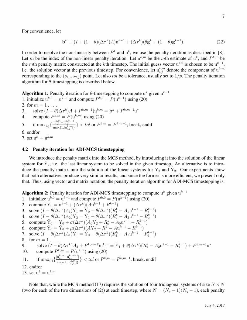
Algorithm 1: Penalty iteration for θ-timestepping to compute uk given uk−1
1. initialize uk,0 = uk−1 and compute P k,0 = P (uk−1) using (20)
2. for m = 1 , . . .
3. solve (I − θ(∆τk)A + P k,m−1)uk,m = bk + P k,m−1u∗
4. compute P k,m = P (uk,m) using (20)
5. if maxi,j{|uk,mi,j −u
k,m−1
i,j |
max{1,|uk,mi,j |}} < tol or P k,m = P k,m−1, break, endif
6. endfor
7. set uk = uk,m
4.2 Penalty iteration for ADI-MCS timestepping
We introduce the penalty matrix into the MCS method, by introducing it into the solution of the linear
system for Y2, i.e. the last linear system to be solved in the given timestep. An alternative is to intro-
duce the penalty matrix into the solution of the linear systems for Y2 and Y2. Our experiments show
that both alternatives produce very similar results, and since the former is more efficient, we present only
that. Thus, using vector and matrix notation, the penalty iteration algorithm for ADI-MCS timestepping is:
Algorithm 2: Penalty iteration for ADI-MCS timestepping to compute uk given uk−1
1. initialize uk,0 = uk−1 and compute P k,0 = P (uk−1) using (20)
2. compute Y0 = uk−1 + (∆τk)(Auk−1 +Rk−1)3. solve (I − θ(∆τk)A1)Y1 = Y0 + θ(∆τk)(Rk
1 −A1uk−1 − Rk−1
1 )4. solve (I − θ(∆τk)A2)Y2 = Y1 + θ(∆τk)(Rk
2 −A2uk−1 − Rk−1
2 )5. compute Y0 = Y0 + σ(∆τk)(A0Y2 +Rk
0 −A0uk−1 − Rk−1
0 )6. compute Y0 = Y0 + µ(∆τk)(AY2 +Rk − Auk−1 − Rk−1)7. solve (I − θ(∆τk)A1)Y1 = Y0 + θ(∆τk)(Rk
1 −A1uk−1 − Rk−1
1 )8. for m = 1 , . . .
9. solve (I − θ(∆τk)A2 + P k,m−1)uk,m = Y1 + θ(∆τk)(Rk2 − A2u
k−1 − Rk−1
2 ) + P k,m−1u∗
10. compute P k,m = P (uk,m) using (20)
11. if maxi,j{|uk,mi,j −u
k,m−1
i,j |
max{1,|uk,mi,j |}} < tol or P k,m = P k,m−1, break, endif
12. endfor
13. set uk = uk,m
Note that, while the MCS method (17) requires the solution of four tridiagonal systems of size N ×N(two for each of the two dimensions of (2)) at each timestep, where N = (Nx − 1)(Ny − 1), each penalty
July 4, 2017
8
iteration requires the solution of only one tridiagonal system of size N ×N (Line 9 of Algorithm 2), after
computing the solution of three tridiagonal systems of size N × N outside the iteration loop. Thus the
number of tridiagonal solutions at the kth timestep of MCS with penalty iteration is 3 + nitk, where nitkis the number of penalty iterations in the kth timestep. Note that the above ADI-MCS penalty technique is
implicit, just as the method proposed in [8] for θ-timestepping, and different from the method in [9]. An
extensive numerical study of the convergence of various techniques for handling the early exercise bound-
ary of American options is found in [14]. It is also worth noting, that our technique of incorporating the
ADI-MCS method into the discrete penalty iteration method for two-dimensional problems, can easily be
extended to higher dimensional problems. For example, for a D-dimensional problem, the MCS method
(for the linear problem) requires the solution of 2D tridiagonal systems of size N × N at each timestep,
while, with the penalty iteration technique (for the nonlinear problem), it requires 2D−1+nitk solutions
of tridiagonal systems, at each timestep.
5 Numerical Results
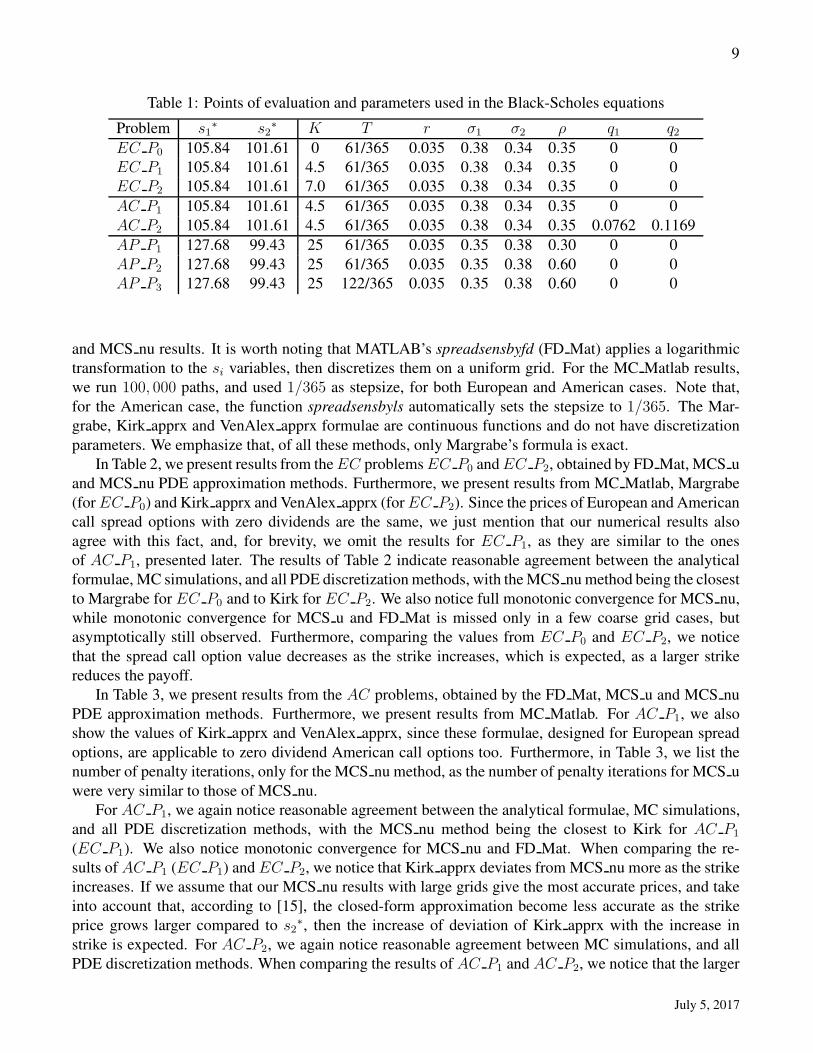
Table 1 displays the parameter values of the test cases we considered. In Table 1, s1∗ and s2
∗ are
points of evaluations. For all cases, the right boundaries are set to S1 = 8s1∗ and S2 = 8s2
∗. The test
cases starting with EC, AC and AP denote European Call, American Call and American Put problems,
respectively. Most of the parameter values for the EC and AC problems are taken from example 3 in
[18], and we vary some of these parameters, in order to better study the behaviour of our method. For the
EC problems, we vary the strike; Problem AC P1 has the same parameter values as EC P1, and, for this
no dividend case, the American and the European call spread options are expected to have the same price;
Problem AC P2 is the same as AC P1, with the exception of non-zero dividends. Most of the parameter
values for the AP problems are taken from example 2 in [18], and we vary some of these parameters, in
order to better study the behaviour of our method. In Problem AP P2, we increase the correlation level
compared to AP P1, and in problem AP P3, we also increase the maturity time.
We present results from two instances of our ADI-MCS method, one using uniform (MCS u), and
another using non-uniform (MCS nu) space grid. In the non-uniform implementation, for each of the two
spatial dimensions, we concentrate more points around the respective coordinate of the evaluation point,
using the smooth mapping function of uniform to non-uniform points (see [3], [2])
f(s) =(
1 +sinh(b(s− a))
sinh(ba)
)
K, (23)
with a ≈ 0.38, and adjusted so that the strike falls on a gridpoint, and b chosen so that the last gridpoint
falls exactly at the right boundary. We used θ = 1, σ = θ, µ = 0.5 − θ for the MCS parameters, and
p = 10−5 for the penalty parameter.
We compare the ADI-MCS results, whenever appropriate, with the results derived using various
other methods, such as other PDE approximation methods, analytical formulae, or MC simulations.
More specifically, for comparison purposes, we use the PDE ADI-DR method of MATLAB [7], [5]
(FD Mat, function spreadsensbyfd), applicable to both European and American spread options, MAT-
LAB’s MC simulations (MC Matlab, function spreadsensbyls), also applicable to both European and
American spread options, Margrabe’s formula [17] applicable only to European exchange options and giv-
ing the exact value, and the analytical approximations by Kirk (Kirk apprx) [15] and Venkatramanan and
Alexander (VenAlex apprx) [22], applicable only to European spread options (or American call spread op-
tions with zero dividends). The FD Mat results presented are for the same grid resolutions as the MCS u
July 4, 2017
9
Table 1: Points of evaluation and parameters used in the Black-Scholes equations
Problem s1∗ s2
∗ K T r σ1 σ2 ρ q1 q2EC P0 105.84 101.61 0 61/365 0.035 0.38 0.34 0.35 0 0
EC P1 105.84 101.61 4.5 61/365 0.035 0.38 0.34 0.35 0 0
EC P2 105.84 101.61 7.0 61/365 0.035 0.38 0.34 0.35 0 0
AC P1 105.84 101.61 4.5 61/365 0.035 0.38 0.34 0.35 0 0
AC P2 105.84 101.61 4.5 61/365 0.035 0.38 0.34 0.35 0.0762 0.1169
AP P1 127.68 99.43 25 61/365 0.035 0.35 0.38 0.30 0 0
AP P2 127.68 99.43 25 61/365 0.035 0.35 0.38 0.60 0 0
AP P3 127.68 99.43 25 122/365 0.035 0.35 0.38 0.60 0 0
and MCS nu results. It is worth noting that MATLAB’s spreadsensbyfd (FD Mat) applies a logarithmic
transformation to the si variables, then discretizes them on a uniform grid. For the MC Matlab results,
we run 100, 000 paths, and used 1/365 as stepsize, for both European and American cases. Note that,
for the American case, the function spreadsensbyls automatically sets the stepsize to 1/365. The Mar-
grabe, Kirk apprx and VenAlex apprx formulae are continuous functions and do not have discretization
parameters. We emphasize that, of all these methods, only Margrabe’s formula is exact.
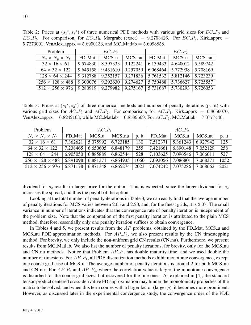
In Table 2, we present results from the EC problems EC P0 and EC P2, obtained by FD Mat, MCS u
and MCS nu PDE approximation methods. Furthermore, we present results from MC Matlab, Margrabe
(for EC P0) and Kirk apprx and VenAlex apprx (for EC P2). Since the prices of European and American
call spread options with zero dividends are the same, we just mention that our numerical results also
agree with this fact, and, for brevity, we omit the results for EC P1, as they are similar to the ones
of AC P1, presented later. The results of Table 2 indicate reasonable agreement between the analytical
formulae, MC simulations, and all PDE discretization methods, with the MCS nu method being the closest
to Margrabe for EC P0 and to Kirk for EC P2. We also notice full monotonic convergence for MCS nu,
while monotonic convergence for MCS u and FD Mat is missed only in a few coarse grid cases, but
asymptotically still observed. Furthermore, comparing the values from EC P0 and EC P2, we notice
that the spread call option value decreases as the strike increases, which is expected, as a larger strike
reduces the payoff.
In Table 3, we present results from the AC problems, obtained by the FD Mat, MCS u and MCS nu
PDE approximation methods. Furthermore, we present results from MC Matlab. For AC P1, we also
show the values of Kirk apprx and VenAlex apprx, since these formulae, designed for European spread
options, are applicable to zero dividend American call options too. Furthermore, in Table 3, we list the
number of penalty iterations, only for the MCS nu method, as the number of penalty iterations for MCS u
were very similar to those of MCS nu.
For AC P1, we again notice reasonable agreement between the analytical formulae, MC simulations,
and all PDE discretization methods, with the MCS nu method being the closest to Kirk for AC P1
(EC P1). We also notice monotonic convergence for MCS nu and FD Mat. When comparing the re-
sults of AC P1 (EC P1) and EC P2, we notice that Kirk apprx deviates from MCS nu more as the strike
increases. If we assume that our MCS nu results with large grids give the most accurate prices, and take
into account that, according to [15], the closed-form approximation become less accurate as the strike
price grows larger compared to s2∗, then the increase of deviation of Kirk apprx with the increase in
strike is expected. For AC P2, we again notice reasonable agreement between MC simulations, and all
PDE discretization methods. When comparing the results of AC P1 and AC P2, we notice that the larger
July 5, 2017
10
Table 2: Prices at (s1∗, s2
∗) of three numerical PDE methods with various grid sizes for EC P0 and
EC P2. For comparison, for EC P0, Margrabe (exact) = 9.2753426. For EC P2, Kirk apprx =5.7273001, VenAlex apprx = 5.6950133, and MC Matlab = 5.6998858.
Problem EC P0 EC P2
Nx ×Ny ×Nt FD Mat MCS u MCS nu FD Mat MCS u MCS nu
32 × 16 × 61 9.574830 8.597333 9.122241 6.139433 4.640012 5.589742
64 × 32 × 122 9.645158 9.431610 9.257059 6.068464 5.772938 5.708169
128 × 64 × 244 9.312788 9.352157 9.271836 5.761532 5.812146 5.723239
256 × 128 × 488 9.300076 9.292630 9.274627 5.750488 5.736627 5.725557
512 × 256 × 976 9.280919 9.279982 9.275167 5.731687 5.730293 5.726053
Table 3: Prices at (s1∗, s2
∗) of three numerical methods and number of penalty iterations (p. it) with
various grid sizes for AC P1 and AC P2. For comparison, for AC P1, Kirk apprx = 6.8656070,
VenAlex apprx = 6.8242103, while MC Matlab = 6.8589669. For AC P2, MC Matlab = 7.0777440.
Problem AC P1 AC P2
Nx ×Ny ×Nt FD Mat MCS u MCS nu p. it FD Mat MCS u MCS nu p. it
32 × 16 × 61 7.362621 5.075992 6.723185 130 7.512371 5.361243 6.927942 125
64 × 32 × 122 7.238465 6.650605 6.848179 255 7.421661 6.890148 7.052129 258
128 × 64 × 244 6.905050 6.885889 6.862544 528 7.103625 7.096546 7.066011 527
256 × 128 × 488 6.891098 6.881371 6.864935 1060 7.093056 7.086801 7.068371 1052
512 × 256 × 976 6.871178 6.871348 6.865274 2023 7.074242 7.075286 7.068662 2021
dividend for s2 results in larger price for the option. This is expected, since the larger dividend for s2increases the spread, and thus the payoff of the option.
Looking at the total number of penalty iterations in Table 3, we can easily find that the average number
of penalty iterations for MCS varies between 2.05 and 2.20, and, for the finest grids, it is 2.07. The small
variance in number of iterations indicates that the convergence rate of penalty iteration is independent of
the problem size. Note that the computation of the first penalty iteration is attributed to the plain MCS
method, therefore, essentially only one penalty iteration suffices to obtain convergence.
In Tables 4 and 5, we present results from the AP problems, obtained by the FD Mat, MCS u and
MCS nu PDE approximation methods. For AP P1, we also present results by the CN timestepping
method. For brevity, we only include the non-uniform grid CN results (CN nu). Furthermore, we present
results from MC Matlab. We also list the number of penalty iterations, for brevity, only for the MCS nu
and CN nu methods. Notice that Problem AP P3 has double maturity time, and we used double the
number of timesteps. For AP P1, all PDE discretization methods exhibit monotonic convergence, except
one coarse grid case of MCS u. The average number of penalty iterations is around 2 for both MCS nu
and CN nu. For AP P2 and AP P3, where the correlation value is larger, the monotonic convergence
is disturbed for the coarse grid sizes, but recovered for the fine ones. As explained in [4], the standard
tensor-product centered cross-derivative FD approximation may hinder the monotonicity properties of the
matrix to be solved, and when this term comes with a larger factor (larger ρ), it becomes more prominent.
However, as discussed later in the experimental convergence study, the convergence order of the PDE
July 4, 2017
11
Table 4: Prices at (s1∗, s2
∗) and number of penalty iterations (p. it) of four numerical methods with various
grid sizes for AP P1. For comparison, MC Matlab = 6.42514245.
Nx ×Ny ×Nt FD Mat MCS u MCS nu p. it CN nu p. it
32 × 16 × 61 7.537957 5.023413 6.244111 134 6.246340 141
64 × 32 × 122 6.758517 6.378849 6.382559 269 6.382566 303
128 × 64 × 244 6.491617 6.432238 6.398929 540 6.398665 552
256 × 128 × 488 6.416549 6.414472 6.401766 1033 6.401568 1031
512 × 256 × 976 6.407908 6.405585 6.402309 2005 6.402195 1996
Table 5: Prices at (s1∗, s2
∗) and number of penalty iterations (p. it) of three numerical methods with
various grid sizes for AP P2 and AP P3. For comparison, for AP P2, MC Matlab = 4.5322051, and for
AP P3, MC Matlab = 6.9451714.
Problem AP P2 AP P3
Nx ×Ny ×Nt FD Mat MCS u MCS nu p. it Nt FD Mat MCS u MCS nu p. it
32 × 16 × 61 6.326957 4.277741 4.524914 131 122 8.371589 7.277957 6.941974 232
64 × 32 × 122 5.185030 5.166896 4.542905 260 244 7.538642 7.677932 6.956781 504
128 × 64 × 244 4.716645 4.865245 4.531880 527 488 7.073126 7.243086 6.941153 1015
256 × 128 × 488 4.565280 4.654163 4.527039 1100 976 6.973622 7.038208 6.934672 2076
512 × 256 × 976 4.537528 4.564074 4.525580 2124 1952 6.942077 6.962628 6.932875 4076
methods is still almost 2. Furthermore, the average number of penalty iterations per timestep remains
approximately 2, i.e. one extra tridiagonal solution is needed per timestep for MCS, besides the four
tridiagonal solutions of the main MCS method.
We next present an experimental study of the convergence of the three PDE approximation methods,
FD Mat, MCS u and MCS nu. For European exchange (zero strike spread) options, i.e. Problem EC P0,
Margrabe’s formula [17] gives the exact value, so we can calculate the exact error for any approximation
method. For European spread options (with non-zero strike), there is no exact formula. We emphasize
that PDE approximation methods exhibit the property of converging to the solution as the discretization
is refined and more computational power is utilized, with the convergence being limited mainly by the
machine precision. The analytical approximations do not possess this property. They are of more limited
accuracy, and, therefore, we do not expect the PDE discretization methods to asymptotically converge
to any of the analytical approximations, such as Kirk apprx or VenAlex apprx. Computing the error as
the difference of a numerical solution from another state of-the-art numerical method or a closed form
approximation carries the problem that we are not guaranteed that the reference solution is more accurate
than our numerical solution.
Considering this, for all the test cases except European exchange options, the error at a particular grid
resolution is estimated by the difference (change) of the solution value with that grid resolution from the
solution value with the previous (coarser) grid resolution.
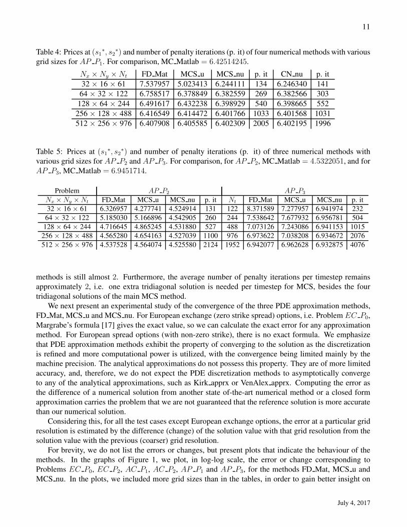
For brevity, we do not list the errors or changes, but present plots that indicate the behaviour of the
methods. In the graphs of Figure 1, we plot, in log-log scale, the error or change corresponding to
Problems EC P0, EC P2, AC P1, AC P2, AP P1 and AP P3, for the methods FD Mat, MCS u and
MCS nu. In the plots, we included more grid sizes than in the tables, in order to gain better insight on
July 4, 2017
12
32 46 64 90 128 180 256 360 512N
x
10 -4
10 -3
10 -2
10 -1
10 0
erro
r(E
C_P
0)
Matlab-DRMCS-uniformMCS-nonuniform
46 64 90 128 180 256 360 512N
x
10 -4
10 -3
10 -2
10 -1
10 0
chan
ge(E
C_P
2)
Matlab-DRMCS-uniformMCS-nonuniform
46 64 90 128 180 256 360 512N
x
10 -4
10 -3
10 -2
10 -1
10 0
chan
ge(A
C_P
1)
Matlab-DRMCS-uniformMCS-nonuniform
46 64 90 128 180 256 360 512N
x
10 -4
10 -3
10 -2
10 -1
10 0ch
ange
(AC
_P2)
Matlab-DRMCS-uniformMCS-nonuniform
46 64 90 128 180 256 360 512N
x
10 -4
10 -3
10 -2
10 -1
10 0
chan
ge(A
P_P
1)
Matlab-DRMCS-uniformMCS-nonuniform
46 64 90 128 180 256 360 512N
x
10 -4
10 -3
10 -2
10 -1
10 0
chan
ge(A
P_P
3)
Matlab-DRMCS-uniformMCS-nonuniform
Figure 1: Log-log scale graphs of the error or change vs. grid size Nx for different test case problems.
July 4, 2017
13
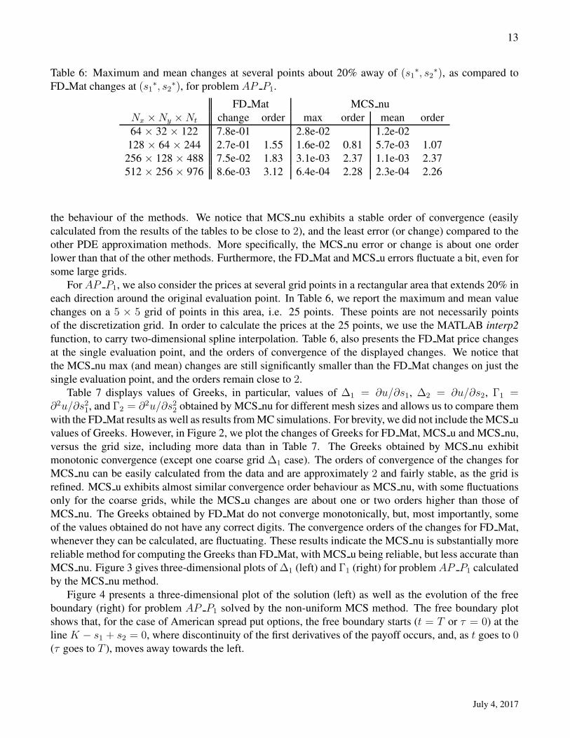
Table 6: Maximum and mean changes at several points about 20% away of (s1∗, s2
∗), as compared to
FD Mat changes at (s1∗, s2
∗), for problem AP P1.
FD Mat MCS nu
Nx ×Ny ×Nt change order max order mean order
64 × 32 × 122 7.8e-01 2.8e-02 1.2e-02
128 × 64 × 244 2.7e-01 1.55 1.6e-02 0.81 5.7e-03 1.07
256 × 128 × 488 7.5e-02 1.83 3.1e-03 2.37 1.1e-03 2.37
512 × 256 × 976 8.6e-03 3.12 6.4e-04 2.28 2.3e-04 2.26
the behaviour of the methods. We notice that MCS nu exhibits a stable order of convergence (easily
calculated from the results of the tables to be close to 2), and the least error (or change) compared to the
other PDE approximation methods. More specifically, the MCS nu error or change is about one order
lower than that of the other methods. Furthermore, the FD Mat and MCS u errors fluctuate a bit, even for
some large grids.
For AP P1, we also consider the prices at several grid points in a rectangular area that extends 20% in
each direction around the original evaluation point. In Table 6, we report the maximum and mean value
changes on a 5 × 5 grid of points in this area, i.e. 25 points. These points are not necessarily points
of the discretization grid. In order to calculate the prices at the 25 points, we use the MATLAB interp2
function, to carry two-dimensional spline interpolation. Table 6, also presents the FD Mat price changes
at the single evaluation point, and the orders of convergence of the displayed changes. We notice that
the MCS nu max (and mean) changes are still significantly smaller than the FD Mat changes on just the
single evaluation point, and the orders remain close to 2.
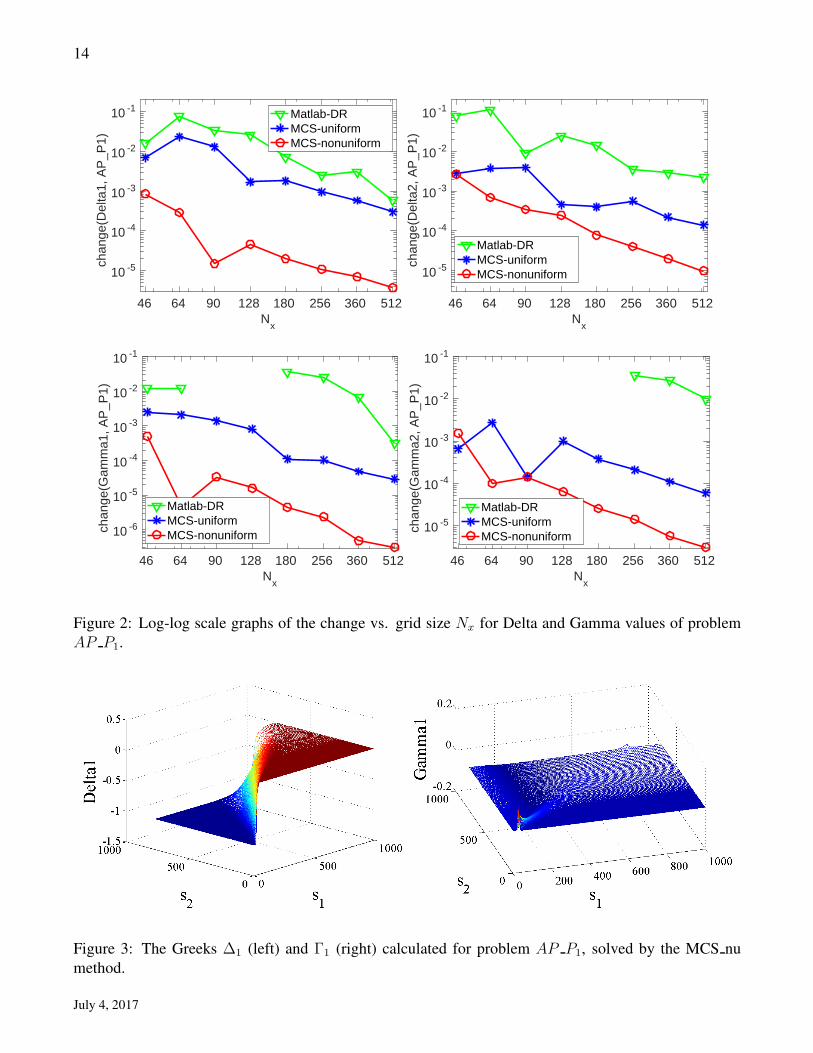
Table 7 displays values of Greeks, in particular, values of ∆1 = ∂u/∂s1, ∆2 = ∂u/∂s2, Γ1 =∂2u/∂s21, and Γ2 = ∂2u/∂s22 obtained by MCS nu for different mesh sizes and allows us to compare them
with the FD Mat results as well as results from MC simulations. For brevity, we did not include the MCS u
values of Greeks. However, in Figure 2, we plot the changes of Greeks for FD Mat, MCS u and MCS nu,
versus the grid size, including more data than in Table 7. The Greeks obtained by MCS nu exhibit
monotonic convergence (except one coarse grid ∆1 case). The orders of convergence of the changes for
MCS nu can be easily calculated from the data and are approximately 2 and fairly stable, as the grid is
refined. MCS u exhibits almost similar convergence order behaviour as MCS nu, with some fluctuations
only for the coarse grids, while the MCS u changes are about one or two orders higher than those of
MCS nu. The Greeks obtained by FD Mat do not converge monotonically, but, most importantly, some
of the values obtained do not have any correct digits. The convergence orders of the changes for FD Mat,
whenever they can be calculated, are fluctuating. These results indicate the MCS nu is substantially more
reliable method for computing the Greeks than FD Mat, with MCS u being reliable, but less accurate than
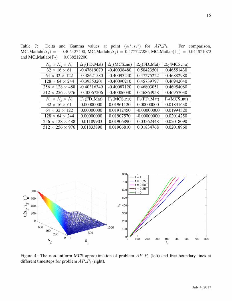
MCS nu. Figure 3 gives three-dimensional plots of ∆1 (left) and Γ1 (right) for problem AP P1 calculated
by the MCS nu method.
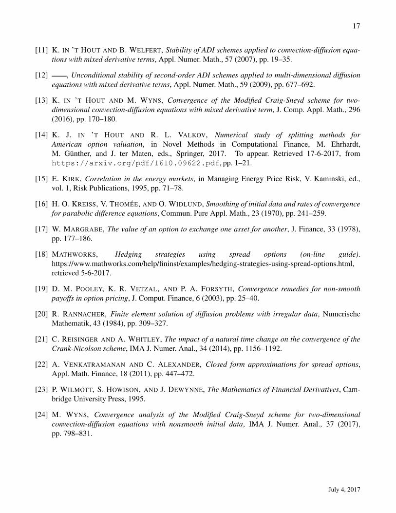
Figure 4 presents a three-dimensional plot of the solution (left) as well as the evolution of the free
boundary (right) for problem AP P1 solved by the non-uniform MCS method. The free boundary plot
shows that, for the case of American spread put options, the free boundary starts (t = T or τ = 0) at the
line K − s1 + s2 = 0, where discontinuity of the first derivatives of the payoff occurs, and, as t goes to 0(τ goes to T ), moves away towards the left.
July 4, 2017
14
46 64 90 128 180 256 360 512N
x
10 -5
10 -4
10 -3
10 -2
10 -1ch
ange
(Del
ta1,
AP
_P1)
Matlab-DRMCS-uniformMCS-nonuniform
46 64 90 128 180 256 360 512N
x
10 -5
10 -4
10 -3
10 -2
10 -1
chan
ge(D
elta
2, A
P_P
1)
Matlab-DRMCS-uniformMCS-nonuniform
46 64 90 128 180 256 360 512N
x
10 -6
10 -5
10 -4
10 -3
10 -2
10 -1
chan
ge(G
amm
a1, A
P_P
1)
Matlab-DRMCS-uniformMCS-nonuniform
46 64 90 128 180 256 360 512N
x
10 -5
10 -4
10 -3
10 -2
10 -1
chan
ge(G
amm
a2, A
P_P
1)
Matlab-DRMCS-uniformMCS-nonuniform
Figure 2: Log-log scale graphs of the change vs. grid size Nx for Delta and Gamma values of problem
AP P1.
Figure 3: The Greeks ∆1 (left) and Γ1 (right) calculated for problem AP P1, solved by the MCS nu
method.
July 4, 2017
15
Table 7: Delta and Gamma values at point (s1∗, s2
∗) for AP P1. For comparison,
MC Matlab(∆1) = −0.405427490, MC Matlab(∆2) = 0.477727230, MC Matlab(Γ1) = 0.044671072and MC Matlab(Γ2) = 0.038212200.
Nx ×Ny ×Nt ∆1(FD Mat) ∆1(MCS nu) ∆2(FD Mat) ∆2(MCS nu)
32 × 16 × 61 -0.47619079 -0.40038480 0.50423501 0.46551430
64 × 32 × 122 -0.38621580 -0.40093240 0.47275222 0.46882980
128 × 64 × 244 -0.39353201 -0.40090210 0.45739797 0.46942040
256 × 128 × 488 -0.40316349 -0.40087120 0.46803051 0.46954080
512 × 256 × 976 -0.40067206 -0.40086030 0.46864958 0.46957030
Nx ×Ny ×Nt Γ1(FD Mat) Γ1(MCS nu) Γ2(FD Mat) Γ2(MCS nu)
32 × 16 × 61 0.00000000 0.01961120 0.00000000 0.01831630
64 × 32 × 122 0.00000000 0.01912450 -0.00000000 0.01994320
128 × 64 × 244 0.00000000 0.01907570 -0.00000000 0.02014250
256 × 128 × 488 0.01189903 0.01906890 0.03562448 0.02018090
512 × 256 × 976 0.01833890 0.01906810 0.01834768 0.02018960
0
500
1000
0200
400600
0
200
400
600
800
s1
s2
u(s 1, s
2, tn)
0 100 200 300 400 500 600 700 8000
100
200
300
400
500
600
700
800
s1
s 2
t = Tt = 0.75Tt = 0.50Tt = 0.25Tt = 0
Figure 4: The non-uniform MCS approximation of problem AP P1 (left) and free boundary lines at
different timesteps for problem AP P1 (right).
July 4, 2017
16
6 Summary
The pricing of European and American spread options was considered using a two-dimensional Black-
Scholes PDE model, solved by an ADI-MCS method. The ADI-MCS method, especially when imple-
mented with a non-uniform grid, is shown to be a competitive timestepping technique for spread option
pricing. In the case of American spread options, a penalty iteration technique is proposed for the handling
of the early exercise feature. We explain how to bind the penalty iteration technique efficiently with ADI-
MCS. The number of tridiagonal system solutions on top of those of the ADI-MCS method required due
to the penalty iteration is essentially one per timestep, irrespectively of grid size. The way we incorporated
ADI-MCS into the penalty iteration can be straightforward extended to problems of higher dimensions.
Our numerical experiments demonstrate that, for European exchange options, we obtain second order
convergence to the exact value given by Margrabe’s formula. For other spread options, we obtain second
order convergence behavior for price values and the Greeks, as well as smooth solutions, Greeks, and free
boundary lines. The ADI-MCS results demonstrate reasonable agreement with those of MC simulations,
MATLAB’s ADI-DR, as well as with those obtained by Kirk’s formula, with the changes of ADI-MCS
prices from one grid resolution to a finer one being at least an order smaller than the MATLAB ADI-DR
ones, and the changes of ADI-MCS Greeks being several orders smaller than the MATLAB ADI-DR
ones.
References
[1] M. BRENNAN AND E. SCHWARTZ, The valuation of the American put option, J. Finance, 32 (1977),
pp. 449–462.
[2] C. C. CHRISTARA AND D. M. DANG, Adaptive and high-order methods for valuing American
options, J. Comput. Finance, 14 (2011), pp. 73–113.
[3] N. CLARKE AND K. PARROTT, Multigrid for American option pricing with stochastic volatility,
Appl. Math. Finance, 6 (1999), pp. 177–195.
[4] S. S. CLIFT AND P. A. FORSYTH, Numerical solution of two asset jump diffusion models for option
valuation, Appl. Numer. Math., 58 (2008), pp. 743–782.
[5] I. CRAIG AND A. SNEYD, An alternating-direction implicit scheme for parabolic equations with
mixed derivatives, Comp. Math. Appl., 16 (1988), pp. 341–350.
[6] J. DOUGLAS AND H. RACHFORD, On the numerical solution of heat conduction problems in two
and three space variables, Trans. Amer. Math. Society, 82 (1956), pp. 421–439.
[7] G. FAIRWEATHER AND A. R. MITCHELL, A new computational procedure for A.D.I. methods,
SIAM J. Numer. Anal., 4 (1967), pp. 163–170.
[8] P. A. FORSYTH AND K. R. VETZAL, Quadratic convergence for valuing American options using a
penalty method, SIAM J. Sci. Comput., 23 (2002), pp. 2095–2122.
[9] T. HAENTJENS AND K. J. IN ’T HOUT, ADI schemes for pricing American options under the Heston
model, Appl. Math. Finance, 22 (2015), pp. 207–237.
[10] S. IKONEN AND J. TOIVANEN, Pricing American options using LU decomposition, Appl. Math.
Sci., 1 (2007), pp. 2529–2551.
July 4, 2017
17
[11] K. IN ’T HOUT AND B. WELFERT, Stability of ADI schemes applied to convection-diffusion equa-
tions with mixed derivative terms, Appl. Numer. Math., 57 (2007), pp. 19–35.
[12] , Unconditional stability of second-order ADI schemes applied to multi-dimensional diffusion
equations with mixed derivative terms, Appl. Numer. Math., 59 (2009), pp. 677–692.
[13] K. IN ’T HOUT AND M. WYNS, Convergence of the Modified Craig-Sneyd scheme for two-
dimensional convection-diffusion equations with mixed derivative term, J. Comp. Appl. Math., 296
(2016), pp. 170–180.
[14] K. J. IN ’T HOUT AND R. L. VALKOV, Numerical study of splitting methods for
American option valuation, in Novel Methods in Computational Finance, M. Ehrhardt,
M. Gunther, and J. ter Maten, eds., Springer, 2017. To appear. Retrieved 17-6-2017, from
https://arxiv.org/pdf/1610.09622.pdf, pp. 1–21.
[15] E. KIRK, Correlation in the energy markets, in Managing Energy Price Risk, V. Kaminski, ed.,
vol. 1, Risk Publications, 1995, pp. 71–78.
[16] H. O. KREISS, V. THOMEE, AND O. WIDLUND, Smoothing of initial data and rates of convergence
for parabolic difference equations, Commun. Pure Appl. Math., 23 (1970), pp. 241–259.
[17] W. MARGRABE, The value of an option to exchange one asset for another, J. Finance, 33 (1978),
pp. 177–186.
[18] MATHWORKS, Hedging strategies using spread options (on-line guide).
https://www.mathworks.com/help/fininst/examples/hedging-strategies-using-spread-options.html,
retrieved 5-6-2017.
[19] D. M. POOLEY, K. R. VETZAL, AND P. A. FORSYTH, Convergence remedies for non-smooth
payoffs in option pricing, J. Comput. Finance, 6 (2003), pp. 25–40.
[20] R. RANNACHER, Finite element solution of diffusion problems with irregular data, Numerische
Mathematik, 43 (1984), pp. 309–327.
[21] C. REISINGER AND A. WHITLEY, The impact of a natural time change on the convergence of the
Crank-Nicolson scheme, IMA J. Numer. Anal., 34 (2014), pp. 1156–1192.
[22] A. VENKATRAMANAN AND C. ALEXANDER, Closed form approximations for spread options,
Appl. Math. Finance, 18 (2011), pp. 447–472.
[23] P. WILMOTT, S. HOWISON, AND J. DEWYNNE, The Mathematics of Financial Derivatives, Cam-
bridge University Press, 1995.
[24] M. WYNS, Convergence analysis of the Modified Craig-Sneyd scheme for two-dimensional
convection-diffusion equations with nonsmooth initial data, IMA J. Numer. Anal., 37 (2017),
pp. 798–831.
July 4, 2017