analytical solution for the stationary model of pollutant
TRANSCRIPT

Ambiente & Água - An Interdisciplinary Journal of Applied Science
ISSN 1980-993X – doi:10.4136/1980-993X
www.ambi-agua.net
E-mail: [email protected]
This is an Open Access article distributed under the terms of the Creative Commons
Attribution License, which permits unrestricted use, distribution, and reproduction in any
medium, provided the original work is properly cited.
Analytical solution for the stationary model of pollutant propagation
in an aquatic medium
ARTICLES doi:10.4136/ambi-agua.2298
Received: 13 Jul. 2018; Accepted: 11 Jan. 2019
Cíntia Ourique Monticelli1* ; Jorge Rodolfo Zabadal2 ;
Daniela Muller Quevedo1 ; Carlos Augusto Nascimento1
1Universidade FEEVALE (FEEVALE), Novo Hamburgo, RS, Brasil
Instituto de Ciências Exatas e Tecnológicas (ICET). E-mail: [email protected],
[email protected], [email protected] 2Universidade Federal do Rio Grande do Sul (UFRGS), Tramandaí, RS, Brasil
Departamento Interdisciplinar. E-mail: [email protected] *Corresponding author
ABSTRACT This work presents a new analytical approach for solving pollutant dispersion problems
along irregular-shaped water bodies. In this approach, the advection-diffusion equation is
expressed in terms of orthogonal curvilinear coordinates, defined by the velocity potential and
the corresponding stream function for inviscid flows. The boundary condition rewritten in terms
of these new coordinates is reduced to a classical third kind one, i.e., the derivative of the
concentration distribution with respect to the stream function is proportional to the numerical
value of the local pollutant concentration. The solution obtained from the proposed formulation
was employed to simulate pollutant dispersion (thermotolerant coliforms) along the Pampa
Creek, a tributary of the Sinos River at the outskirts of Novo Hamburgo city, South Region of
Brazil. The results obtained reproduce the qualitative behavior of the expected concentration
distribution.
Keywords: advection-diffusion equation, analytical solutions, mass transport, orthogonal curvilinear
coordinates system, pollutant dispersion.
Solução analítica do modelo estacionário de propagação de poluentes
em meio aquático
RESUMO Este trabalho apresenta uma nova abordagem analítica para a solução de problemas de
dispersão de poluentes ao longo de corpos hídricos com contornos irregulares. Nesta
abordagem, a equação advectivo-difusiva é expressa em termos de coordenadas curvilíneas
ortogonais que são definidas pelo potencial de velocidade e pela função de corrente
correspondente para fluídos invíscivos. A condição de contorno reescrita em termos destas
novas coordenadas é reduzida a uma de terceira espécie clássica, isto é, a derivada da
distribuição de concentração em relação à função de corrente é proporcional ao valor numérico
da concentração de poluente local. A solução obtida a partir da formulação proposta foi
empregada para simular dispersão de poluentes (coliformes termotolerantes) ao longo do Arroio
Pampa, afluente do rio dos Sinos, na periferia de Novo Hamburgo, cidade do sul do Brazil. Os

Rev. Ambient. Água vol. 14 n. 2, e2298 - Taubaté 2019
2 Cíntia Ourique Monticelli et al.
resultados obtidos reproduzem o comportamento qualitativo da distribuição de concentração
esperada.
Palavras-chave: dispersão de poluentes, equação advectivo-difusiva, sistema de coordenadas
curvilíneas ortogonais, soluções analíticas, transporte mássico.
1. INTRODUCTION
The conservation of surface water quality is of great importance for society, since this
water is collected in order to supply public distribution systems. However, due to their power
of dilution and self-purification, several rivers also serve as the final destination of sanitary
sewage. Hence, the technical tools to aid in the planning, monitoring and management of water
resources, among which mathematical modeling stands out as a fundamental instrument, are
very important. Mathematical models allow the generation of properly organized data, spatially
and temporally integrating dispersed data, as well as promoting a better understanding of the
dynamics of the processes and a prediction of future conditions of the system regarding relevant
parameters.
Rivers are the main source of water for human consumption. Thus, controlling the water
quality of the rivers is very important because water is directly related to human health (Qishlaqi
et al., 2017). In environmental impact studies of sewage transport network projects, part of the
data to be produced is the determination of a safe distance from the vicinal area or points of raw
water collection for water treatment plants, where effluents can be discharged through an
emissary so that the dispersion plume does not reach these areas. Surely, one can also estimate
the contamination level that would be produced if the pollutant inevitably reached the regions
of interest.
To obtain reliable results regarding the distance of the sewage outfall in relation to the
source and to the point of water collection, and thus minimize the total costs of an enterprise, it
is necessary to carry out several computational simulations. These simulations would be able
to predict the approximate spatial distribution of pollutant concentrations considering a large
quantity of scenarios by using mathematical models for mass transport. However, the time
required by computational programs capable of implementing such models can become a
critical point for certain applications that require a high level of detail, since the large number
of mathematical calculations in a commonly used numerical model (Rosman, 2001), (Gomes
et al., 2018) causes delays in the generation of the results.
The governing equation of pollutant transmission in rivers is the advection diffusion
equation (ADE). This is a partial equation that is very important in environmental engineering,
and several hydraulic phenomena such pollution transmission, suspended sediment transport
modeling, etc. are involved (Parsaie and Haghiabi, 2017). The ADE includes two differential
parts, advection and diffusion; the advection part characterizes the velocity´s contribution in
the pollutant transmission, and the diffusion or dispersion part characterizes the molecular
transmission from highest concentration region to lowest concentration region. In addition to
the differential terms present in ADE, there are the physical parameters which will be described
throughout this work.
Three possible solutions could be proposed to solve the differential equation that describe
the problem in question: the numerical, analytical and hybrid methods. Numerical methods,
usually employed by the scientific community, often provide sufficiently realistic results for
particle transport problems (Jobim, 2012). In the application of numerical solutions to
computational fluid dynamics, either by applying the finite difference, finite element or finite
volume methods and artificial neural network - ANN (Parsaie and Haghiabi, 2017), it is
common to have to discretize the domain into a mesh with thousands or even millions of points.

3 Analytical solution for the stationary model of …
Rev. Ambient. Água vol. 14 n. 2, e2298 - Taubaté 2019
This may produce algebraic systems of a very high order (Fernandez, 2007); thus, in most cases,
the numerical solutions demand a high computational effort. Consequently, they require a high
processing time, which may make it impossible in some cases to generate a sufficient number
of scenarios in a timely manner.
In order to avoid these problems, the use of analytical solutions is more advantageous. As
they are expressed in closed form, it is possible to write small source codes that are executed in
a shorter processing time, which is due to the decrease in the number of operations to be
performed and, consequently, in the memory required for all the necessary routines. The
advection-diffusion equation, which describes the transport of particles, has several proposed
analytical solutions, such as the integral transform method (Mikhailov and Ozisik, 1984), the
generalized integral transform method (Cotta, 1993), the change of variables combined with
the integral transform method (Guerrero et al., 2009), using the Green´s function (Sanskrityayn
and Kumar, 2016), among others. However, changes in the geometry of the domain are not
considered, whereas this would be required in the problem of transporting particles in a water
body.
This study presents a new analytical approach to solve the problem of pollutant dispersion
in the aquatic environment, in which the advection-diffusion equation is expressed in terms of
new orthogonal curvilinear coordinates, defined by the velocity potential and by the stream
function. Such reformulation aims to standardize the boundary conditions to be prescribed, in
addition to considerably increasing the size of the elements of the corresponding mesh. The use
of this technique produces a closed solution for the propagation model of conservative or non-
conservative pollutants and its implementation generates very compact symbolic codes and
high computational performance.
In addition, the that way the physical parameters, present in the ADE, are obtained has
fundamental importance. The determination of the longitudinal dispersion coefficients that
properly describes the stream behavior is one of the main objectives of research works, like
those of Paisaie et al. (2018) Haghiabi (2016; 2017), that use different techniques to obtain
them. In the solution proposed by this study, the dispersion coefficients used are the ones
obtained by Garcia in 2009 and the velocity coefficients obtained by Lersh et al. in 2013.
In order to prove the feasibility and validity of the proposed method, we present the results
of a one-dimensional model for the simulation of dispersion of organic pollutants
(thermotolerant coliforms) in a 7 km-stretch of the Pampa Creek until its mouth in the Sinos
River – located in an urban area of the city of Novo Hamburgo, Rio Grande do Sul, Brazil.
2. MATERIAL AND METHODS
2.1. Equations Model
In this study, in order to obtain an approximation for estimating the concentration of
thermotolerant coliforms downstream from a point source, the flow was considered to be:
homogeneous, isotropic, uniform, incompressible and irrotational. That is, respectively:
absence of regions with “superconcentrations” or even actions of fields that interact with the
substance of interest, absence of the characteristic that causes the molecule to migrate from one
point to another that differ in each direction of pollutant propagation, and the pressure and
turbulence temperature conditions are approximately the same at all points. The velocity field
has divergent zero, i.e., there are no diffusive terms nor generation or decay. And finally,
considering the irrotational flow to be the viscosity effects forming the hydrodynamic boundary
layer on the banks of the river, they can be neglected and the fluid considered with viscosity
equal to zero, which does not constitute vorticity.
Yet, many rivers and lakes can be reduced to a two-dimensional problem by behaving like
water slides, since the depth is much smaller than the distance between the boundaries, so the

Rev. Ambient. Água vol. 14 n. 2, e2298 - Taubaté 2019
4 Cíntia Ourique Monticelli et al.
dispersion would have enough time to homogenize the vertical concentration profile at the
moment the plume has spread horizontally on a geographic scale. Consequently, the dispersion
in the z-direction will be neglected.
With the changes and simplifications applied to the general equation of the particle balance
(Cranck, 1975; Kambe, 2007) based on an Eulerian view of the process, and assuming that the
kinetics of reactions could be represented by a first-order decay, the two-dimensional
advection-diffusion equation for non-conservative pollutants is given as Equation 1:
𝜕𝐶
𝜕𝑡+ 𝑢
𝜕𝐶
𝜕𝑥+ 𝑣
𝜕𝐶
𝜕𝑦= 𝐷 (
𝜕2𝐶
𝜕𝑥2+
𝜕2𝐶
𝜕𝑦2) − 𝑘𝐶 (1)
In Equation 1, 𝐶 is the pollutant concentration, 𝑥 and 𝑦 are the directions of motion, 𝑢 and
𝑣are the velocities of the water body in the directions 𝑥 and 𝑦 respectively, 𝐷 is the surface
oscillation diffusion coefficient (Garcia et al., 2009) and 𝑘 is the coefficient of velocity.
When one intends to estimate the level of pollution caused by the discharge of sewage
systems in different regions of a watercourse, whether for classification and framing according
to current regulations or for the projection of bathing conditions, it is desirable to generate
results that express the system in its steady state. Since the time scale in which the dispersion
occurs is much higher than the characteristic period of the thermal and hydrodynamic
fluctuations of the flow, the time evolution pattern of the diffusion, kinetic and velocity field
coefficients present stationarity, that is, low amplitude stochastic oscillations around a fixed
mean value. In this study, the coefficients of diffusion and velocity shall be considered constant,
representing temporal arithmetic means independent of time.
Since the only transient effect on the concentration distribution to be considered is due to
the effects of degradation kinetics, which is a phenomenon independent of mass transport,
Equation 1 can be decoupled through the split process (Zabadal and Ribeiro, 2012):
In the kinetic Equation 2:
𝜕𝐶
𝜕𝑡= −𝑘𝐶 (2)
And in the transport Equation 3:
𝑢𝜕𝐶
𝜕𝑥+ 𝑣
𝜕𝐶
𝜕𝑦= 𝐷 (
𝜕2𝐶
𝜕𝑥2+
𝜕2𝐶
𝜕𝑦2) (3)
2.2. Analytical Solution
With the target equation decoupled in a system of two equations, Equation 2 and Equation
3, they can be solved in parallel.
2.2.1. Solution of the kinetic equation for first-order decay
The asymptotic behavior of the kinetic model for most pollutants is exponential, thus
solving Equation 2 by separation of variables we obtain Equation 4:
𝐶(𝑥, 𝑦, 𝑡) = 𝑓(𝑥, 𝑦)𝑒−𝑘𝑡 (4)
The function 𝑓(𝑥, 𝑦) is precisely the exact solution for the transport equation, Equation 3.
Thus, substituting Equation 5 into Equation 3 restored the transport equation:
(𝑢𝜕𝑓
𝜕𝑥+ 𝑣
𝜕𝑓
𝜕𝑦)= 𝐷 (
𝜕2𝑓
𝜕𝑥2 +𝜕2𝑓
𝜕𝑦2) (5)

5 Analytical solution for the stationary model of …
Rev. Ambient. Água vol. 14 n. 2, e2298 - Taubaté 2019
2.3. Solution of transport equation for point sources
It is possible to produce the solution of the transport equation by writing it in terms of a
new curvilinear coordinate system (𝜙, 𝜓) and, only then, solve it. To perform this task, initially,
it is necessary to redefine the first and second order partial derivatives of the function 𝑓(𝑥, 𝑦)
in terms of the velocity potential 𝜙(𝑥, 𝑦) and the stream function 𝜓(𝑥, 𝑦). By using the chain
rule (Equations 6 and 7):
𝜕𝑓
𝜕𝑥=
𝜕𝑓
𝜕𝜙
𝜕𝜙
𝜕𝑥+
𝜕𝑓
𝜕𝜓
𝜕𝜓
𝜕𝑥 (6)
𝜕𝑓
𝜕𝑦=
𝜕𝑓
𝜕𝜙
𝜕𝜙
𝜕𝑦+
𝜕𝑓
𝜕𝜓
𝜕𝜓
𝜕𝑦 (7)
And the identities and conditions of Cauchy-Riemann Equation 8:
𝑢 =𝜕𝜙
𝜕𝑥 =
𝜕𝜓
𝜕𝑦 , 𝑣 =
𝜕𝜙
𝜕𝑦= −
𝜕𝜓
𝜕𝑥 (8)
Writing the write the second-order derivative, regrouping the terms and making the
necessary simplifications, the Laplacian of 𝑓(𝑥, 𝑦) is yielded in terms of the new coordinates
𝜙 and 𝜓 Equation 9:
𝛻2𝑓(𝑥, 𝑦) = (𝑢2 + 𝑣2) (𝜕2𝑓
𝜕𝜙2 +𝜕2𝑓
𝜕𝜓2) +𝜕𝑓
𝜕𝜙((𝑢
𝜕𝑢
𝜕𝜙− 𝑣
𝜕𝑢
𝜕𝜓) + (𝑣
𝜕𝑣
𝜕𝜙+ 𝑢
𝜕𝑣
𝜕𝜓)) +
𝜕𝑓
𝜕𝜓((𝑣
𝜕𝑢
𝜕𝜙+ 𝑢
𝜕𝑢
𝜕𝜓) −
(𝑢𝜕𝑣
𝜕𝜙− 𝑣
𝜕𝑣
𝜕𝜓)) (9)
The partial derivatives of the velocity field components 𝑢 and 𝑣can be defined with the
help of the chain rule, thus Equations 10 and 11:
𝜕𝑢
𝜕𝑥= 𝑢
𝜕𝑢
𝜕𝜙− 𝑣
𝜕𝑢
𝜕𝜓 and
𝜕𝑢
𝜕𝑦= 𝑣
𝜕𝑢
𝜕𝜙+ 𝑢
𝜕𝑢
𝜕𝜓 (10)
𝜕𝑣
𝜕𝑥= 𝑢
𝜕𝑣
𝜕𝜙− 𝑣
𝜕𝑣
𝜕𝜓 and
𝜕𝑣
𝜕𝑦= 𝑣
𝜕𝑣
𝜕𝜙+ 𝑢
𝜕𝑣
𝜕𝜓 (11)
Once the relations Equation 10 and Equation 11 had replaced into Equation 9, the divergent
and rotational of the velocity field will be cancelled, since incompressible and irrotational flows
are being considered. This allows us to rewrite the diffusion terms of the target Equation 12 as:
𝛻2𝑓(𝑥, 𝑦) = (𝑢2 + 𝑣2) (𝜕2𝑓
𝜕𝜙2 +𝜕2𝑓
𝜕𝜓2) (12)
In order to complete the procedure, it is also necessary to rewrite the advection terms of
Equation 5 as a function of the new coordinates Equation 13:
𝑢𝜕𝑓
𝜕𝑥+ 𝑣
𝜕𝑓
𝜕𝑦= 𝑢 (𝑢
𝜕𝑓
𝜕𝜙− 𝑣
𝜕𝑓
𝜕𝜓) + 𝑣 (𝑣
𝜕𝑓
𝜕𝜙+ 𝑢
𝜕𝑓
𝜕𝜓) = (𝑢2 + 𝑣2)
𝜕𝑓
𝜕𝜙+ (𝑢𝑣 − 𝑣𝑢)
𝜕𝑓
𝜕𝜓 (13)
Finally, the advection-diffusion equation for the steady state can be explained as a function
of the new coordinate system. Equating the two sides in Equation 12 and Equation 13 and
dividing by (𝑢2 + 𝑣2), Equation 5 is thus rewritten as a function of curvilinear coordinates
Equation 14:

Rev. Ambient. Água vol. 14 n. 2, e2298 - Taubaté 2019
6 Cíntia Ourique Monticelli et al.
𝜕𝑓
𝜕𝜙= 𝐷 (
𝜕2𝑓
𝜕𝜙2 +𝜕2𝑓
𝜕𝜓2) (14)
The Equation 14, that describes the bi-dimensional model, can be solved by using
Bäcklund (Polyanin and Zaitzev, 2004) and Fourier transformations (Spiegel, 1976). However,
in this study, due to the restricted number of experimental data, we will consider the one-
dimensional problem.
2.4. One-dimensional Model
In the case of narrow or slow-flow rivers, as soon as the concentration distribution reaches
the steady state the cross profile will be homogenized. Therefore, the diffusion term in this
direction, (𝜕2𝑓
𝜕𝜓2), can be neglected and the model will become one-dimensional, described
through the ordinary differential Equation 15:
𝑑𝑓
𝑑𝜙= 𝐷
𝑑2𝑓
𝑑𝜙2 (15)
Solving Equation 16 by the method of separation of variables and a second integration, the
result is:
𝑓(𝜙) = 𝑏0 + 𝑐𝑜𝑒𝜙
𝐷 (16)
In this solution b0 represents a constant buffer, namely, the minimum value of
concentration that the substance of interest will reach, which can be considered null for non-
conservative pollutants, since for these the concentration C will fall to zero when 𝜙→ -∞ in the
absence of new sources. The constant 𝑐0 represents the initial concentration of the contaminant
at the point of discharge.
Reacting the solution obtained by Equation 17 to the solution of the kinetic equation given
by Equation 4, we obtain:
𝐶 = 𝑐0𝑒(𝜙
𝐷−𝑘𝑡)
(17)
Expression Equation 17 results in the concentration of the pollutant downstream from the
point source given that the initial concentration of the pollutant and its velocity profile in the
stretch are known.
3. RESULTS AND DISCUSSION
3.1. Experimental data
In order to validate the proposed solution, experimental data were used (Nascimento and
Naime, 2009). The data were collected at the source, main body and mouth of the Pampa Creek,
an affluent of the Sinos River, shown in Figure 1. The Sinos River supplies approximately 97%
of the urban population of the city of Novo Hamburgo in Rio Grande do Sul, Brazil (COMUSA,
2015). This city has an estimated population of 249,113 inhabitants (IBGE, 2017). Pampa Creek
receives a domestic load from a region with approximately 40% of the total population of the
city (Novo Hamburgo, 2017). Their effluents are discharged in the stream without any
treatment, subsequently flowing into the Sinos River for about 1.5 km to the water collection
point for treatment and subsequent public distribution for the city.
Point P1, located at the source of the Pampa Creek, has been taken as the starting point of
the particles. Point P2, located midstream the course of Pampa is 3919 m away from P1, as well
as P3, the mouth of the creek, which is located at 7669 m away from P1. Point P4, on the Sinos

7 Analytical solution for the stationary model of …
Rev. Ambient. Água vol. 14 n. 2, e2298 - Taubaté 2019
River, located next to the raw water pumping station of the water treatment plant is 1668m
downstream of P3.
Although the model described here has the ability to change the geometry under study,
once the coordinate system has been modified, we intend to validate the results based on the
one-dimensional approach given by Equation 17. For validation of the two-dimensional
solution, Equation 14, it is necessary to obtain a more robust amount of data, such as pollutant
concentration and velocity in more than one line along the water body.
Figure 1. Pampa creek´s location and data collection points.
The next figures show that the expression found as a problem solution (Equation 17) is
experimental data adherent. The mean values for the thermotolerant coliforms measured from
May 2006 to August 2006, and from January 2007 to March 2007, are presented, respectively,
in Figures 2 and 3. We choose these periods because they had a similar precipitation profile.
The samples were collected at the source of the Pampa Creek (P1), midstream along the course
(P2), at the mouth of the brook (P3) and at the raw water collection point for water treatment in
the Sinos River (P4), on eight different dates, at the four points of interest. The mean values
show that the profile of coliform concentration from the data collected experimentally presents
exponential decay, as suggested by the solution.
Figure 2. Average coliform concentration profile, from May to
August 2006 at the 4 sampling points.

Rev. Ambient. Água vol. 14 n. 2, e2298 - Taubaté 2019
8 Cíntia Ourique Monticelli et al.
Figure 3. Average coliform concentration profile, from
January to March 2007 at the 4 sampling points.
3.2. Velocity Potentials
The hydraulic variables are directly related to the watercourse flow. Thus, during rainy
periods, and more frequently throughout autumn and winter, in this region of the country the
flow velocity increases, as well as the level of the watercourse. Consequently, the depth and
width of the water resource, along with the drainage area, increase.
The velocities at the four points selected for this study were obtained with the Flo-MateTM
portable speed meter Model 2000. Monthly measurements were performed at each of the points
and are described in Tables 1, 2 and 3. The mean velocity was used in each point and period of
interest.
At the raw water collection point by the Municipal Company of Sanitation of Novo
Hamburgo (COMUSA), P4, the mean velocity of the watercourse was used for the
spring/summer period, which was measured at 0.37m/s, and for the fall/winter period, 0.69m/s.
The 𝜙(𝑥) coordinate values were calculated at each point and date considering the mean
value of flow velocity, 𝑢, by the definition of the velocity potential (Equation 18):
𝜙(𝑥)𝑖 = 𝛼 ∫ �̅�𝑑𝑥−𝑋𝑖
0 (18)
In Equation 18, 𝛼 = 10−4 represents a dimensionless correction value at the order of
magnitude of the velocity to contemplate the effect that the stirring of the liquid mass exerts on
the velocity measurement float, since it moves in all directions in very short intervals of time.
This effect causes considerable amplifications on the diffusion coefficient as it promotes an
essentially isotropic mixture when the shells formed on the surface of the water rise and fall
alternately. Thus, it is not necessary to calculate the effective distance traveled over time
accumulating the projections of the velocity vector on the main direction of the flow. The
diffusion coefficient for the stagnant water (Brownian motion), for which the order of
magnitude is 0.000001 (Bird et al., 2002), is then divided by the diffusion coefficient –
estimated by means of an oscillatory model derived from Navier-Stokes equations (model
Korteweg-de Vries), the value of which is approximately 0.01 (Garcia et al., 2009). Thus, this
quotient is on the order of 10-4. Note that this quotient equals the product between the
instantaneous velocity and half of the mean free course.
Table 1. Measured velocity and velocity potentials at P1.
Period May/06 Jul/06 Aug/06 Oct/06 Nov/06 Jan/07 Mar/07 May/07
𝑢(m/s) 0.081 0.10 0.175 0.149 0.134 0.062 0.154 0.12
𝜙(𝑥)(m2/s) 0 0 0 0 0 0 0 0

9 Analytical solution for the stationary model of …
Rev. Ambient. Água vol. 14 n. 2, e2298 - Taubaté 2019
Table 2. Measured velocity and velocity potentials at P2.
Period May/06 Jul/06 Aug/06 Oct/06 Nov/06 Jan/07 Mar/07 May/07
𝑢(m/s) 0.23 0.102 0.376 0.326 0.392 0.367 0.394 0.39
𝜙(𝑥)(m2/s) -0.0966 -0.03997 -0.1435 -0.1279 -0.15391 -0.14393 -0.15441 -0.15284
Table 3. Measured velocity and velocity potentials at P3.
Period May/06 Jul/06 Aug/06 Oct/06 Nov/06 Jan/07 Mar/07 May/07
𝑢(m/s) 0.03 0.456 0.28 0.4518 0.063 0.221 0.242 0.18
𝜙(𝑥)(m2/s) -0.02301 -0.34971 -0.21473 -0.3465 -0.04875 -0.16948 -0.18559 -0.13804
3.3. Coefficient of diffusion
In the absence of any other characteristic that might make the probability of a molecule to
migrate from one point to another be different for each direction of propagation of the pollutant,
it is safe to assume that the diffusion coefficient is a constant value. Thus, the coefficient of
diffusion by surface oscillation in microscale, 𝐷, was given by the quotient between the mean
free courses and double the period between successive molecular collisions, in which
D = 0.25m2/s (Garcia et al., 2009).
3.4. Coefficient of velocity
The coefficient of velocity, k, presented in the model referring to the kinetics of bacterial
and chemical pollutants decay, is indirectly dependent on the position and on the time variable.
This dependency is due to the velocity constant being influenced by factors that can vary both
in space and time, such as temperature, turbulence and wind incidence, which cause oscillations
on the surface of the water body, in addition to the pollutant concentration itself.
For the determination of , the data for the calculation of another coefficient, T90, was used.
This coefficient was obtained through laboratory assays and measures the time required to
reduce the level of bacteria present in water by 90%, i.e., to reduce the concentration to 10% of
the original value at the point of emission. In the experiment (Lersch et al., 2013), this reduction
occurred in 48h, which, based on the solution of the first order differential equation that
describes the degradation kinetics, allowed us to estimate that the rate constant in
k = -0.0479.
3.5. Time
The time has been calculated based on the distance that the particle traveled in each section
and the mean velocity obtained experimentally. For each section, on each different date, the
mean travel time was calculated. Given the ease of calculation by the reader and the great
amount of information, no further explanations on this specific topic will be given, since there
are eight different dates and four different points of the course evaluated.
3.6. Simulations
By using all the described data, it was possible to simulate the dispersion of thermotolerant
coliforms based on the hypothesis that they are discharged at a specific location in the Pampa
Stream and dispersed along its course.
The results of the simulations are presented on the different dates in which the samples
were collected. Point P1 was taken as a source of pollutant discharge near the source of the
stream and the amount of coliforms remaining at point P2 (midstream) was then simulated.
Figure 4 presents the results obtained in the simulations and the measured values distributed in
a scatter plot. In this graph, the complete agreement of the results with the experimental data is
not shown, since this area is a highly urbanized zone, so point P1 is certainly not the only source
of load in this stretch.
Rev. Ambient. Água vol. 14 n. 2, e2298 - Taubaté 2019
10 Cíntia Ourique Monticelli et al.
Figure 4. Experimental and simulated data. Discharge influence of
P1 in P2.
Considering P2 as a point source of discharge, the amount of thermotolerant coliforms
remaining at point P3, that is, at the mouth of the stream, was simulated. This result was
presented in Figure 5, which shows a better agreement of the data obtained through the
simulation and the values measured experimentally, due to the order of magnitude of the
parameter involved.
Figure 5. Experimental and simulated data. Discharge influence
of P2 in P3.
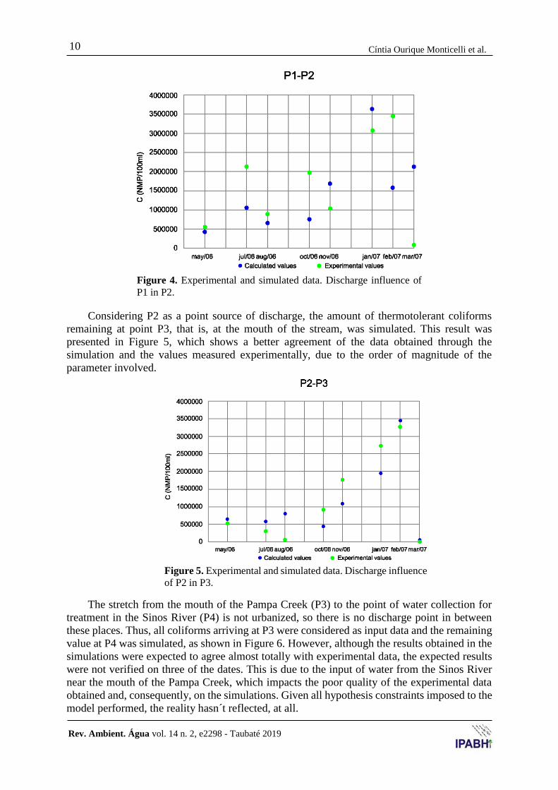
The stretch from the mouth of the Pampa Creek (P3) to the point of water collection for
treatment in the Sinos River (P4) is not urbanized, so there is no discharge point in between
these places. Thus, all coliforms arriving at P3 were considered as input data and the remaining
value at P4 was simulated, as shown in Figure 6. However, although the results obtained in the
simulations were expected to agree almost totally with experimental data, the expected results
were not verified on three of the dates. This is due to the input of water from the Sinos River
near the mouth of the Pampa Creek, which impacts the poor quality of the experimental data
obtained and, consequently, on the simulations. Given all hypothesis constraints imposed to the
model performed, the reality hasn´t reflected, at all.
11 Analytical solution for the stationary model of …
Rev. Ambient. Água vol. 14 n. 2, e2298 - Taubaté 2019
Figure 6. Experimental and simulated data. Discharge Influence ofP3
in P4.
The points P1, P2 and P3 are in the same watercourse, the Pampa Stream, whereas P4 is
located in the course of the Sinos River, where the water flow and velocity change considerably.
Thus, the difference between the calculated values and the respective experimental data is
basically due to two causes of error: flow inversion and considerable fluctuations in the velocity
field. Both factors are observed, frequently in periods of high flow rates, as was the case when
experimental data were obtained. Since the hydrodynamic model employed considers the flow
to be potential, implicitly the hypothesis of steady state is assumed. Therefore, any perturbation
that produces transients in the velocity field had been neglected in the proposed model.
Moreover, even the most refined hydrodynamic formulations based on the Navier-Stokes and
Helmholtz equations (Bird et al., 2002; Mott, 2006) produce equally disparate results, since it
is not possible to reproduce such fluctuations with fidelity, but only to estimate their amplitudes
and frequencies in a relatively coarse manner. Haghiabi et al. (2018) examining models of
artificial neural networks (ANN) and support vector machine (SVM), showed that all of them
had some over-estimation properties. In short, the simplified hydrodynamic model is, in
practice, as realistic as the finer formulations in fluid mechanics, even though they contemplate
turbulence models.
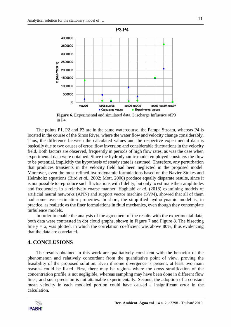
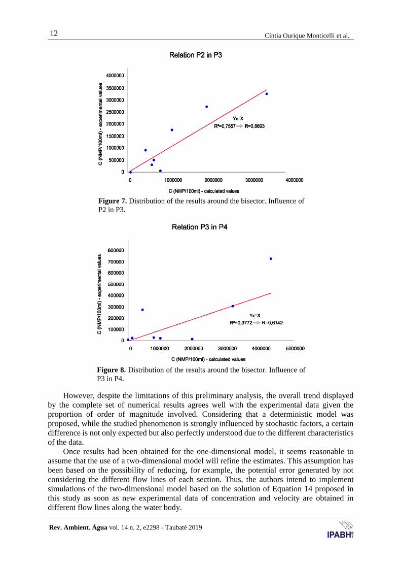
In order to enable the analysis of the agreement of the results with the experimental data,
both data were contrasted in dot cloud graphs, shown in Figure 7 and Figure 8. The bisecting
line y = x, was plotted, in which the correlation coefficient was above 80%, thus evidencing
that the data are correlated.
4. CONCLUSIONS
The results obtained in this work are qualitatively consistent with the behavior of the
phenomenon and relatively concordant from the quantitative point of view, proving the
feasibility of the proposed solution. Even if some divergence is present, at least two main
reasons could be listed. First, there may be regions where the cross stratification of the
concentration profile is not negligible, whereas sampling may have been done in different flow
lines, and such precision is not attainable experimentally. Second, the adoption of a constant
mean velocity in each modeled portion could have caused a insignificant error in the
calculation.
Rev. Ambient. Água vol. 14 n. 2, e2298 - Taubaté 2019
12 Cíntia Ourique Monticelli et al.
Figure 7. Distribution of the results around the bisector. Influence of
P2 in P3.
Figure 8. Distribution of the results around the bisector. Influence of
P3 in P4.
However, despite the limitations of this preliminary analysis, the overall trend displayed
by the complete set of numerical results agrees well with the experimental data given the
proportion of order of magnitude involved. Considering that a deterministic model was
proposed, while the studied phenomenon is strongly influenced by stochastic factors, a certain
difference is not only expected but also perfectly understood due to the different characteristics
of the data.
Once results had been obtained for the one-dimensional model, it seems reasonable to
assume that the use of a two-dimensional model will refine the estimates. This assumption has
been based on the possibility of reducing, for example, the potential error generated by not
considering the different flow lines of each section. Thus, the authors intend to implement
simulations of the two-dimensional model based on the solution of Equation 14 proposed in
this study as soon as new experimental data of concentration and velocity are obtained in
different flow lines along the water body.

13 Analytical solution for the stationary model of …
Rev. Ambient. Água vol. 14 n. 2, e2298 - Taubaté 2019
5. REFERENCES
BIRD, R. B.; STEWART, W. E.; LIGHTFOOT, E. N. Transport Phenomena. 2nd ed. New
York: John Wiley & Sons, 2002.
COMPANHIA MUNICIPAL DE SANEAMENTO DE NOVO HAMBURGO/RS - COMUSA.
Economias abastecidas pela Comusa aumentam 7% nos últimos cinco anos. 2015.
Available in: https://goo.gl/nD4tLN. Access: 21 Apr. 2017.
COTTA, R. M. Integral Transforms in Computational Heat and Fluid Flow. Boca Raton:
CRC Press, 1993.
CRANK, J. The Mathematics of Diffusion. 2nd ed. Bristol: Oxford University Press, 1975.
FERNANDEZ, L. C. Simulação da propagação de poluentes utilizando transformação de
Backlund: modelo bidimensional. 2007. Dissertação (Mestrado em Engenharia
Mecânica) – Universidade Federal do Rio Grande do Sul, Porto Alegre, 2007.
GARCIA, R. L.; ZABADAL, J.; RIBEIRO, V.; POFFAL, C. Definição do coeficiente de
difusão para propagação de poluentes em águas rasas empregando um modelo baseado
em soluções exatas para a equação de Korteweg-de Vries. Vetor, v. 19, n. 1, p. 15-27,
2009.
GOMES, S. H. R., SIQUEIRA, T. M.; GUEDES, H.; ANDREAZZA, R.; HUFFNER, A. N.;
CORRÊA, L. Modelagem sazonal da qualidade da água do Rio dos Sinos/RS utilizando
o modelo QUAL-UFMG. Engenharia Sanitária e Ambiental, v. 23, p. 275-285, 2018.
GUERRERO, J. S.; PIMENTEL, L.; SKAGGS, T.; GENUCHTEN, M. Analytical solution of
the advection–diffusion transport equation using a change-of-variable and integral
transform technique. International Journal of Heat and Mass Transfer, v. 52, p. 3297–
3304, 2009.
HAGHIABI, A. H. Prediction of longitudinal dispersion coefficient using multivariate adaptive
regression splines. Journal of Earth System Science, v. 125, n. 5, p. 985-995, 2016.
HAGHIABI, A. H. Modeling River Mixing Mechanism Using Data Driven Model. Water
Resources Management, v. 31, n. 3, p. 811-824, 2017.
http://dx.doi.org/10.1007/s11269-016-1475-7
HAGHIABI, A. H.; NASROLAHI, A. H.; PARSAIE, A. Water quality prediction using
machine learning methods. Water Quality Research Journal, v. 53, n. 1, 2018.
http://dx.doi.org/10.2166/wqrj.2018.025
IBGE. Infográficos: evolução populacional e pirâmide etária. 2017. Available in:
https://goo.gl/zEUMpm. Access: 21 Apr. 2017.
KAMBE, T. Elementary Fluid Mechanics. Singapore: World Scientific Publishing, 2007.
JOBIM, G. S. Dispersão de poluentes: simulação numérica do Lago Guaíba. 2012. TCC
(Graduação em Engenharia Civil) - Departamento de Engenharia Civil, UFRGS, Porto
Alegre, 2012.
LERS.CH, E. C.; HOFFMANN, C. X.; ROSMAN, P. C. Relatório complementar de
avaliação do impacto ambiental do projeto socioambiental ETE Serraria. Aplicação
de Modelos Matemáticos Transientes. Porto Alegre: DMAE, 2013.

Rev. Ambient. Água vol. 14 n. 2, e2298 - Taubaté 2019
14 Cíntia Ourique Monticelli et al.
MIKHAILOV, M. D.; OZISIK, M. N. Unified Analysis and Solutions of Heat and Mass
Diffusion. New York: John Wiley & Sons, 1984.
MOTT, R. Applied Fluid Mechanics. 6th ed. New Jersey: Prentice Hall, 2006.
NASCIMENTO, C.; NAIME, R. Monitoramento físico-químico das águas do Arroio Pampa
em Novo Hamburgo/RS. Estudos Tecnológicos, v. 5, n. 2, p. 245-269, 2009.
NOVO HAMBURGO. Prefeitura Municipal. Estudos de concepção e projetos básicos de
requalificação urbana e ambiental da sub-bacia do arroio Pampa – Novo Hamburgo
– RS. 2017. Available in: https://goo.gl/VTLLUi. Access: 21 Nov. 2017.
PARSAIE, A.; HAGHIABI, A. H. Computational Modeling of Pollution Transmission in
Rivers. Applied Water Science, v. 7, n. 3, p. 1213-1222, 2017.
http://dx.doi.org/10.1007/s13201-015-0319-6
PARSAIE, A.; EMAMGHOLIZADEH, S.; AZAMATHULLA, H. M.; HAGHIABI, A. H.
ANFIS-based PCA to predict the longitudinal dispersion coefficient in rivers.
International Journal of Hydrology Science and Technology, v. 8, n. 4, p. 410-424,
2018. http://dx.doi.org/10.1504/IJHST.2018.095537
POLYANIN, A.; ZAITZEV, V. Handbook of Nonlinear Partial Differential Equations.
Boca Raton: Chapman & Hall/CRC, 2004.
QISHLAQI, A.; KORDIAN, S.; PARSAIE, A. Hydrochemical evaluation of river water quality
– a case study. Applied Water Science, n. 7, p. 2337-2342, 2017.
http://dx.doi.org/10.1007/s13201-016-0409-0
ROSMAN, P. C. C.; MASCARENHAS, F. C.; MIGUEZ, M.; CAMPOS, R.; EIGER, S. Um
sistema computacional de hidrodinâmica ambiental. In: ABRH. Métodos Numéricos em
Recursos Hídricos. vol. 5. Rio de Janeiro, 2009.
SANSKRITYAYN, A.; KUMAR, N. Analytical solution of advection–diffusion equation in
heterogeneous infinite medium using Green’s function method. Journal of Earth
System Science, v. 125, p. 1713, 2016. https://doi.org/10.1007/s12040-016-0756-0
SPIEGEL, M. R. Fourier Analysis. New York: McGraw-Hill Publications, 1976.
ZABADAL, J. R.; RIBEIRO, V. Equações diferenciais para engenheiros: uma abordagem
prática. Porto Alegre: UniRitter, 2012.