Analysis of Trajectory Flexibility PreservationImpact on Traffic Complexity

Husni R. Idris*, Nola Shen† and Tarek El-Wakil$

L3-Communications, Billerica, MA, 01821

David J. Wing §

NASA Langley Research Center, Hampton, VA, 23681

The growing demand for air travel is increasing the need for mitigation of air trafficcongestion and complexity problems, which are already at high levels. At the same time newinformation and automation technologies are enabling the distribution of tasks and decisionsfrom the service providers to the users of the air traffic system, with potential capacity andcost benefits. This distribution of tasks and decisions raises the concern that independentuser actions will decrease the predictability and increase the complexity of the traffic system,hence inhibiting and possibly reversing any potential benefits. In answer to this concern, theauthors proposed the introduction of decision-making metrics for preserving user trajectoryflexibility. The hypothesis is that such metrics will make user actions naturally mitigatetraffic complexity. In this paper, the impact of using these metrics on traffic complexity isinvestigated. The scenarios analyzed include aircraft in en route airspace with each aircraftmeeting a required time of arrival in a one-hour time horizon while mitigating the risk ofloss of separation with the other aircraft, thus preserving its trajectory flexibility. Theexperiments showed promising results in that the individual trajectory flexibilitypreservation induced self-separation and self-organization effects in the overall trafficsituation. The effects were quantified using traffic complexity metrics, namely dynamicdensity indicators, which indicated that using the flexibility metrics reduced aircraft densityand the potential of loss of separation.

Nomenclature

ADP Adaptability

RBT Robustness

RTA Required Time of Arrival

(t,x,y) (time, x-location, y-location)

V Ground speed

hi , hmin,hmax Heading with its maximum and minimum values

Traj Trajectory

P i Probability of trajectory instance traj i

* Principal Research Engineer, 300 Concord Road, Suite 400, AIAA Member† Research Analyst, 300 Concord Road, Suite 400, AIAA Member$ Software Engineer, 300 Concord Road, Suite 400, AIAA Member§ Principal ATM Research Engineer, Mail Stop 152

https://ntrs.nasa.gov/search.jsp?R=20090029955 2018-07-09T02:22:33+00:00Z

P c Probability of constraint situation c

Pf Probability of feasibility

P f,c Probability of feasibility in constraint situation c

f(t,x,y) Number of feasible trajectories from (t,x,y) to destination

fc(t,x,y) Number of feasible trajectories from (t,x,y) to destination in situation c

i(t,x,y) Number of infeasible trajectories from (t,x,y) to destination

ic(t,x,y) Number of infeasible trajectories from (t,x,y) to destination in situation c

N(t,x,y) Number of all trajectories from (t,x,y) to destination

g(x,y) or gk(x,y) Number of trajectories from k=(t,x,y) to next time step

s Duration between time increments

AT Time horizon for conflict detection

I. Introduction

In order to handle the expected increase in air traffic, the Next Generation Air Transportation System (NextGen)will introduce key transformations in Air Traffic Management (ATM). 1 Three examples are: increasing

information sharing through net-enabled information access; making access to National Airspace System (NAS)resources dependent on aircraft equipage; and aircraft trajectory-based operations enabled by aircraft ability toprecisely follow customized four dimensional (4D) trajectories. 1 These capabilities enable shifting the ATM systemtowards a distributed architecture. 2 For example, NextGen is investigating delegating more responsibility for trafficseparation to the pilot2,3 and delegating more responsibility to airline operation centers for traffic flowmanagement3,4 . Enabling the gains of distributed decision making depends on the ability of distributed actions, byairborne and ground-based agents, to maintain safety and efficiency at acceptable levels.

Research on distributed ATM has focused, in part, on the distribution of separation responsibility between pilotsand controllers. 5,6,7,8,9 Neglecting to regulate traffic beyond the separation assurance time horizon may causecomplex traffic situations, which may be difficult to control whether by ground-based or by aircraft-based agents,leading to compromised safety. Therefore, reducing or preventing such situations is a prerequisite to enablingmanageable separation assurance and safety. In order to mitigate traffic complexity, ground and airborne systemsmay benefit from preserving trajectory flexibility. Trajectory flexibility preservation enables an aircraft to plan itstrajectory such that it preserves a requisite level of maneuvering flexibility in order to accommodate laterdisturbances caused, for example, by other traffic and weather activity. The hypothesis is that if each aircraftpreserves its own trajectory flexibility, using an air-based or ground-based system, acceptable traffic complexity willnaturally be achieved. As discussed in Idris et al., although flexibility preservation does not explicitly coordinatebetween aircraft, it assists each by reducing the risk of conflict due to the potential behavior of the surroundingtraffic, thus resulting in implicit coordination. 1 0,11 This function offers a trajectory-oriented approach to managingtraffic complexity, by explicitly planning aircraft trajectories, such that their contribution to complexity isminimized. This is contrasted with airspace-oriented approaches that aim to ensure that airspace characteristics (suchas sector size and route patterns) and traffic characteristics (such as aircraft density) are designed to dynamicallylimit traffic complexity.

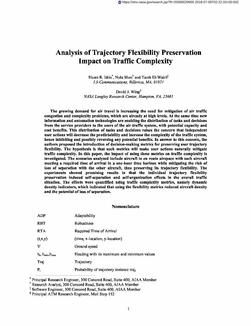
Flexibility preservation complements separation assurance both within the conflict resolution horizon andbeyond it to an extended flexibility planning horizon. Within the conflict resolution horizon, flexibility aids inselecting conflict resolution solutions that afford the aircraft more flexibility, for example, to adapt to potentialintruder behavior. Beyond the conflict resolution horizon, which is the focus of this paper, flexibility preservationplans the aircraft trajectory to minimize its exposure to disturbances such as weather cells and dense traffic. Fig. 1depicts an example. In its left portion each aircraft, while planning its trajectory between weather cells, questionswhether it should modify its trajectory to increase flexibility. If the aircraft proceed along their depicted headings, acomplex traffic situation arises causing excessive congestion and a high potential conflict rate. On the other hand,the right portion displays a structured traffic pattern that would result if each aircraft maneuvered to increase its ownflexibility.

2

Ownship

Flexibility

metric

i

Applicability of Trajectory Flexibility Prediction Trajectories Designed to Preserve Flexibility

Airborne flexibility function will auestion:

Hypothesis:

Do I have enough flexibility to safely proceed?

If all aircraft apply flexibilityCan I modify my trajectory to increase my flexibility?

preservation function, complexity

Do I need to avoid this airspace entirely and replan?

automatically will be reduced

Figure 1 Trajectory flexibility preservation avoiding weather cells and congestion

To test this hypothesis, trajectory flexibility metrics have been defined in previous work to represent robustnessand adaptability to the risk of violating separation, airspace hazards, and traffic flow management constraints. 1 1-13

The impact of trajectory planning by preserving these metrics is analyzed on traffic complexity metrics selectedfrom the literature. Many approaches have been documented to define and measure traffic complexity, most often asa function of controller workload. For example, dynamic density measures traffic complexity using a number offactors. These factors are primarily based on airspace geometry such as aircraft density, sector geometry, traffic flowstructure, and mix of aircraft types and performance characteristics. 14-17 Other efforts emphasized cognitive elementsof complexity, in particular the controller use of standard flows, grouping of traffic, and merge points. 18 Somemetrics have been proposed that are independent of the airspace structure and controller perspective. For example,Delahaye et al. 19 introduced complexity metrics based on traffic organization or disorder based on Lyapunovexponents. In a previous paper20, the impact of preserving trajectory flexibility was analyzed on the Lyapunov-exponent-based metrics. In this paper the impact on dynamic density metrics is analyzed.

Two scenarios are analyzed in two-dimensional en route airspace, where each aircraft must meet a required timeof arrival (RTA) in a one-hour time horizon using speed and heading degrees of freedom. Simultaneously, eachaircraft preserves its trajectory flexibility, using the defined metrics, to mitigate the risk of loss of separation withhazards and the other aircraft. The effects are quantified using traffic complexity metrics based on flow patternconsistency and dynamic density. The experiments showed promising results in terms of mitigating complexity asmeasured by these metrics.

II. Metrics

Metrics that represent trajectory flexibility have been developed and reported in previous papers. 12,13 They aresummarized briefly in this section. To test the hypothesis, traffic complexity metric were also selected. Thesemetrics are also briefly described in this section.

A. Trajectory Flexibility MetricsThe notion of “trajectory flexibility” was defined in Idris et al. 11 as the ability of the trajectory (and hence the

aircraft following the trajectory) to abide by all constraints imposed on it while mitigating its exposure to risks thatcause violation of these constraints. The constraints intend to achieve ATM and aircraft objectives and includeheading limits, RTAs, and separation minima. They define the trajectory solution space. Risk of constraint violationis represented by disturbances that cause the aircraft trajectory to violate or potentially violate constraints.Disturbances were classified in Idris et al. 1 1-13 into state disturbances that result in aircraft state deviation along itstrajectory or constraint disturbances such as new constraints or modifications of currently imposed or knownpotential constraints.

Two trajectory characteristics relevant to measuring this notion of flexibility have been identified: robustnessand adaptability. 11 Metrics have been proposed for robustness and adaptability based on estimating the number offeasible trajectories available to the aircraft to accommodate disturbances. 12,13 They are summarized here briefly. Inorder to support these definitions and estimation methods, the aircraft is assumed to follow segments of discrete timelength, where instantaneous heading and speed changes can only occur at discrete instances in time that are s apart.

Also, heading h and speed V take discrete values between hmin and hmax and between Vmin and Vmax and are constantalong each segment. (Altitude is not considered in this paper.) In addition to simplifying the estimation method,these assumptions are reasonable from an operational point of view considering the intended application of thetrajectory flexibility metrics. Namely, the metrics are intended for relative comparison of trajectories over a longtime horizon suitable for strategic planning (typical of traffic flow management planning horizon) as opposed totactical maneuvering (where the dynamics of the speed and heading change are relevant).

(1)Robustness is defined as the ability of the aircraft to keep its planned trajectory unchanged in response to theoccurrence of disturbances, for example, no matter which trajectory or conflict instances materialize. A robustnessmetric RBT(t, x, y) is measured with the probability of feasibility P f(traj) of the trajectory (traj) starting from a state(t, x, y) and ending at another state such as (RTA, xdest, ydest). Pf(traj) can be estimated with partial information aboutstate and constraint disturbances, modeled with probability distributions that represent the risk of constraintviolation. As an example, the constraints are modeled with C constraint situations c, each with a probability P c

with ∑ Pc = 1. Each constraint situation c divides the total set of trajectories N(t, x, y) into two mutually exclusivec=1:C

subsets: fc(t, x, y) the set of feasible trajectories and i c(t, x, y) the set of infeasible trajectories, both with respect to c.Then, the following ormula can be derived for robustness tRBT x 1213g (, , y); see Idris et al. , for more details:

Pf,c (t,x,y)= ∑ P(traj i ) =fc (t,x,y) RBT(t,x,y) = Pf (t,x,y) =∑ Pc × fc(t,x, Y) (1)set of feasible trajectoryinstances i N(t, x, y) c=1:C fc (t, x, y) + i c (t, x, y)

where Pf,c is the probability of feasibility of the trajectory traj in a constraint situation c, which is the ratio of thenumber of feasible trajectories fc to the total number of trajectories N, if the probability of each trajectory instanceP(traj i) is equal to 1/N(t,x,y).

(2) Adaptability is defined as the ability of the aircraft to change its planned trajectory in response to theoccurrence of a disturbance that renders the current planned trajectory infeasible. An adaptability metric ADP(t, x,y) is measured by the number of feasible trajectories f(t, x, y) (with respect to all constraints) that are available forthe aircraft to use at (t, x, y) to regain feasibility. Then, given the probability distribution (Pc) of each constraintsituation c of C, ADP may be estimated by the average over C:

ADP(t, x, y) = f (t, x, y) = ∑ P × f (t, x, y) (2)c=1:C

Adaptability decreases as the aircraft moves along a trajectory because the number of feasible trajectoriesdecreases. The special case of robustness given by (1) (robustness to totally random state disturbances) increasesover time because as the number of feasible trajectories (numerator) decreases the total number of trajectories(denominator) decreases more rapidly by both infeasible and feasible trajectories.

B. Traffic Complexity MetricsThe impact of planning trajectories using the adaptability and robustness metrics on traffic complexity was

assessed using two main indicators: Consistency of a resulting flow pattern and dynamic density. Flow patternconsistency was measured by the percentage of aircraft that followed a consistent pattern. The pattern was readilyapparent visually so no clustering technique was employed in the scenarios analyzed in this paper. The pattern wasscenario dependent as will be described in Section IV. A number of dynamic density indicators were selected fromthe literature14-17, based on applicability (for example excluding indicators that are based on altitude variation and onsector geometry). The indicators were not combined in a single metric because such combination would reflectspecific operational environment. Rather the indicators were measured and reported independently. The following isa brief description of each of the indicators:

(1) Traffic density is the number of cells (the whole analyzed area is divided into sixty-four cells with equalsize) occupied by more than a certain number of aircrafts for each instant of time.

(2) Horizontal proximity is the inverse of the average weighted horizontal separation between all the aircraftpairs for each instant of time. For each aircraft, the weighted horizontal separation is estimated based on the distanceto all the other aircrafts. Those aircrafts closer to the own aircraft are given more weight. 16

(3) Variance of headings using the standard deviation of the headings of all the aircrafts within a defined area.The area is selected (as described in Section III.B and shown in Fig. 5 and 6) instead of the full area so that theaircraft movement pattern can be reflected in the metric.

(4) The number of conflicts is the number of aircraft pairs with impending conflicts in a time horizon . Themeasure is normalized by the number of aircrafts for each time step. Both aircraft state-based and the trajectory-based conflicts are detected. 10 minutes conflict prediction time horizon was used in this analysis. For state-basedconflicts, the shortest distance between the aircraft pairs is estimated based on their speed, heading and initialseparation. This shortest distance is then compared with the minimum horizontal separation (a 5 nautical mile

4

separation requirement was used) according to a published algorithm21 . The conflict is detected for this aircraft pairif the estimated shortest distance is less than the minimum horizontal separation. The number of conflicts is alsoestimated according to the resulting aircraft trajectories. For each time step, the aircraft pairs with horizontalseparation less than the minimal horizontal separation in the next 10 minutes is counted as impending conflict.

(5) Crossing angle is the average crossing angle of the aircraft pairs with impending conflict in . Thecrossing angle is the acute angle between the paths of two converging aircraft predicted to be in conflict using thestate projection.

(6) Time to conflict is the inverse of average minimum time to the conflict for all the aircrafts with impendingconflicts in . For aircraft state-based conflicts, the time to conflict is the time to the closest approach point. Whilefor the trajectory-based conflicts, the time to conflict is to the time when the aircraft pair first lost the minimumseparation.

III. Trajectory Generation Algorithm

A dynamic programming algorithm was used to generate an aircraft trajectory using the robustness andadaptability metrics. Because the intention of this analysis is to test a hypothesis rather than a real-time application,the dynamic programming approach was selected due to its simple formulation and despite its numerical and storagelimitations. First the trajectory solution space is built as a tree of discrete states connected according to reachabilityby the allowable discrete speed and heading values over the discrete time increments. Second, the robustness andadaptability metrics are estimated at each state. Third and finally, a back-propagation algorithm computes a costfunction and builds a trajectory that optimizes the cost function.

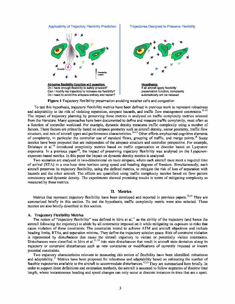
A. Flexibility Metric EstimationUnder the assumptions of discrete

time and degrees of freedom, the Blocked cells due to Reachability of point

number of trajectories was estimated loss of separation k over ε given by gk

using a convolution and filtering y

technique. 11 Fig. 2 demonstrates this ` rmethod for calculating fc(t, x, y) from Grid of : 5 ' }`' ^`` ` Y '` >'' r) ^£0 {,` F

discrete*r

y cells ^' y ' ' • 0'''any point (t, x, y) to a destination x- `` ' ` ` x `' n. , ' t

spec b oint RTA' Y,.

'' ^^ 0`1^ Y a 1^ ( , xdest, ydest) z,. ;`,:

:' ',' 0 n ' ;

and a tolerance circle around it in the ' 'i , t ( 0 Y,:

0 0x-y plane, in a constraint situation c

0 0

that includes an instance of a :`' , x .^ 0

potential conflict. The 3-dimensional G, d ` Initialization of} ►̀ .,' `t v ` r r ' ^^` last time step:

space is discretized into time steps s- f= 1 if insideapart, where in each time step the x-y RTA tolerance, t

plane is discretized into square cells. X '` '' f=0 if outside

The function fc(t, x, y) is estimatedX`"

Point or},.

Time step ε cell kt, r' ,r

for each cell. Assume the function V

fc(tj , x, y) at time tj is known. Thefunction fc(tj-1, x, y) at the previoustime step tj-1 can be obtained by Figure 2. Discrete estimation of number of feasible trajectoriesconvoluting fc(tj , x, y) and thefunction gk(x, y), which represents the number of trajectories that reach from a point k=(tj-1, x(k), y(k)) at time steptj-1 to the next time step tj . The function gk(x, y) is shown as a conical shell in Fig. 2. However, if the point k isinfeasible (for example due to loss of separation) then fc(tj-1, x(k), y(k)) = 0. This requires a filtering step before eachconvolution operation to zero out the values at infeasible states. Substituting a dummy variable i to denote slidingthe point k in the x-y plane, the function fc(tj-1, x, y) is given by the following equation, representing convolution andfiltering for infeasibility:

fc (t j-1, x, y) = Z Z f Jt j Jz A)g(x - z, y - A) if feasibleA z (3)

fc(t j-1, x, y) = 0 if infeasibleThis operation is applied starting from the destination step t = RTA and proceeding backwards to the current

state. The destination time step is initialized by setting f c(RTA, x, y) = 1 at the feasible states and zero elsewhere asshown in Fig. 2. To compute the total number of trajectories, N(t, x, y) used in the denominator of the robustness

metric RBT, certain constraints are excluded from the filtering process (namely the constraints with respect to whichrobustness is computed). In this paper robustness only to loss of separation with traffic and hazards is considered.Therefore, the numerator filtering was applied to all cells that lead to separation loss as well as cells that lead toviolating speed and heading limits or violating the RTA constraint. On the other hand, filtering ignored loss ofseparation but was applied to the RTA and heading and speed limit constraints for calculating the denominator.

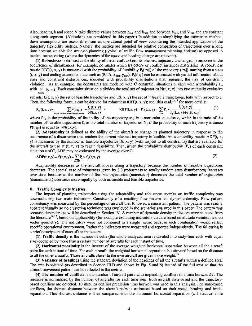
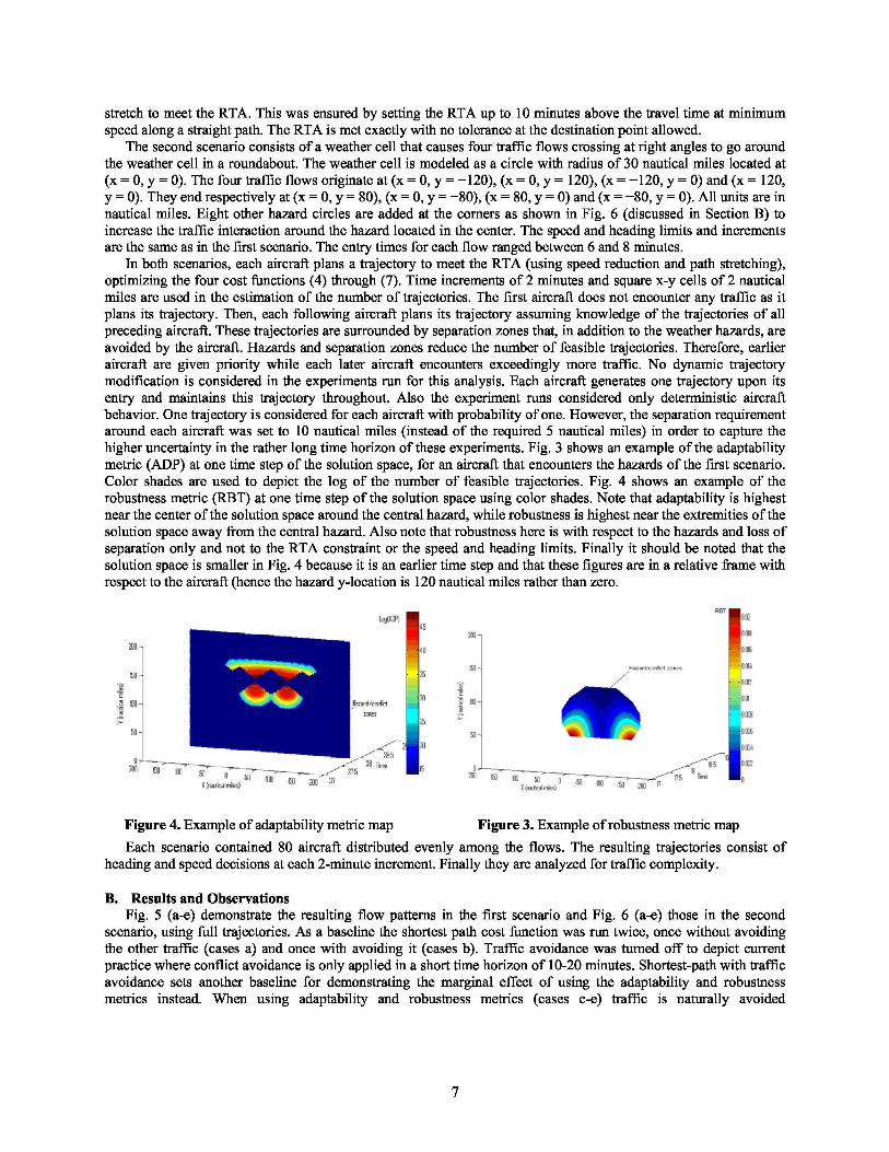
Separation zones were modeled as circles with given radii surrounding each intruder aircraft trajectory. Becausea trajectory consists of discrete segments, each with constant speed and heading, the circle moves with constantspeed and heading for the duration of each segment. In each segment, the circle is enclosed with eight tangentplanes, each two opposing tangents resulting from a combination of heading and speed limits of the ownship aircraftrelative to the intruder (There are four such combinations). A cell loses (or is imminent to lose) separation if it fallson the inside of all eight planes, within the time duration of the segment. Hazards are similarly modeled as circleswith zero speed. Under probabilistic models of disturbances, the estimation process is repeated for each constraintsituation c. Then, the estimates fc(t, x, y) are averaged over all situations C to obtain the adaptability or robustnessmetrics (1) and (2). Examples of ADP and RBT are shown in Fig. 3 and 4 for an analysis case.

B. Cost Function and Trajectory BuildingUsing recursive back-propagation, starting from the final time step, the minimum cost of proceeding from each

cell to the destination is computed and stored. This minimum cost Q(t,x(k),y(k)) for each cell k is computed byminimizing, over its reachable cells given by {(t+1,x,y):gk(t+1,x,y)=1 } in the next time step t+1, the sum of theminimum cost Q(t+1,x,y) already computed for each of the reachable cells (t+1,x,y) plus the cost of proceedingfrom k to that cell, given for short by q(k4(t+1,x,y)). A generic formula is:

Q(t, x(k), y(k)) = x yMin i1{Q(t + 1, x, y) + q(k → (t + 1, x, y)}

Four functions for the local cost q were used in the experiments reported in this paper. A function representingminimizing path length was used as a baseline. Then, functions representing maximizing adaptability, maximizingrobustness, and maximizing both combined with minimizing path length:

q(k → (t + 1, x, y)) = distance(k → (t + 1, x, y)) = dist (4)

q(k → (t + 1, x, y)) = −ADP(k) (5)q(k → (t + 1, x, y)) = −RBT(k) (6)

q(k → (t + 1, x, y)) = −ADP(k) − a T RBT(k) + b Tdist (7)where a and b are weights that trade robustness and distance, respectively, with adaptability. They are raised to thepower of time T (measured from the end) to account for the exponential growth of ADP. After storing the optimalcosts for each cell, a forward loop builds a trajectory by tracing the optimal cells starting from the initial state. Anyties were broken randomly.

IV. Complexity Impact Analysis

The estimation technique and trajectory optimization algorithm were implemented in a MATLAB tool. Theresulting trajectories were analyzed using the traffic complexity metrics described in Section III.B. First thescenarios reported in this paper are described. Then, observations are made on the impact of trajectory planning,using the four cost functions (4) through (7), on traffic complexity.

A. Analysis ScenarioThe first of the two scenarios analyzed in this paper consists of a line of weather cells leaving two holes for

which two flows of traffic compete. The two traffic flows travel in opposite directions: one starts at x = 0, y = —120nautical miles and heads towards x = 0, y = 80 nautical miles. The other flow starts at x = 0, y = 120 and ends at x =0, y = —80 nautical miles. Five weather hazard cells are modeled as circles with radius of 20 nautical miles, andlocated at x = 0 and y = {0, ±70, ±120 nautical miles}. See Fig. 5 in Section B with the results. The geometry of thehazards and of the traffic start and end positions is selected to provide symmetry, such that the path length alone isnot a differentiator between selecting among the two holes. This ensures highlighting the impact of the robustnessand adaptability metrics compared to shortest path. Each traffic flow is generated with random entry times separatedby intervals between 5 and 7 minutes. All aircraft are limited to headings of ±60 degrees relative to the centerlineconnecting the start and end positions, with 10-degree increments. They are also limited to a speed between 240 and360 knots with 10-knot increments. Each aircraft is assigned an RTA at the destination that forces the aircraft to path

6

stretch to meet the RTA. This was ensured by setting the RTA up to 10 minutes above the travel time at minimumspeed along a straight path. The RTA is met exactly with no tolerance at the destination point allowed.

The second scenario consists of a weather cell that causes four traffic flows crossing at right angles to go aroundthe weather cell in a roundabout. The weather cell is modeled as a circle with radius of 30 nautical miles located at(x = 0, y = 0). The four traffic flows originate at (x = 0, y = —120), (x = 0, y = 120), (x = —120, y = 0) and (x = 120,y = 0). They end respectively at (x = 0, y = 80), (x = 0, y = —80), (x = 80, y = 0) and (x = —80, y = 0). All units are innautical miles. Eight other hazard circles are added at the corners as shown in Fig. 6 (discussed in Section B) toincrease the traffic interaction around the hazard located in the center. The speed and heading limits and incrementsare the same as in the first scenario. The entry times for each flow ranged between 6 and 8 minutes.

In both scenarios, each aircraft plans a trajectory to meet the RTA (using speed reduction and path stretching),optimizing the four cost functions (4) through (7). Time increments of 2 minutes and square x-y cells of 2 nauticalmiles are used in the estimation of the number of trajectories. The first aircraft does not encounter any traffic as itplans its trajectory. Then, each following aircraft plans its trajectory assuming knowledge of the trajectories of allpreceding aircraft. These trajectories are surrounded by separation zones that, in addition to the weather hazards, areavoided by the aircraft. Hazards and separation zones reduce the number of feasible trajectories. Therefore, earlieraircraft are given priority while each later aircraft encounters exceedingly more traffic. No dynamic trajectorymodification is considered in the experiments run for this analysis. Each aircraft generates one trajectory upon itsentry and maintains this trajectory throughout. Also the experiment runs considered only deterministic aircraftbehavior. One trajectory is considered for each aircraft with probability of one. However, the separation requirementaround each aircraft was set to 10 nautical miles (instead of the required 5 nautical miles) in order to capture thehigher uncertainty in the rather long time horizon of these experiments. Fig. 3 shows an example of the adaptabilitymetric (ADP) at one time step of the solution space, for an aircraft that encounters the hazards of the first scenario.Color shades are used to depict the log of the number of feasible trajectories. Fig. 4 shows an example of therobustness metric (RBT) at one time step of the solution space using color shades. Note that adaptability is highestnear the center of the solution space around the central hazard, while robustness is highest near the extremities of thesolution space away from the central hazard. Also note that robustness here is with respect to the hazards and loss ofseparation only and not to the RTA constraint or the speed and heading limits. Finally it should be noted that thesolution space is smaller in Fig. 4 because it is an earlier time step and that these figures are in a relative frame withrespect to the aircraft (hence the hazard y-location is 120 nautical miles rather than zero.

Figure 4. Example of adaptability metric map Figure 3. Example of robustness metric map

Each scenario contained 80 aircraft distributed evenly among the flows. The resulting trajectories consist ofheading and speed decisions at each 2-minute increment. Finally they are analyzed for traffic complexity.

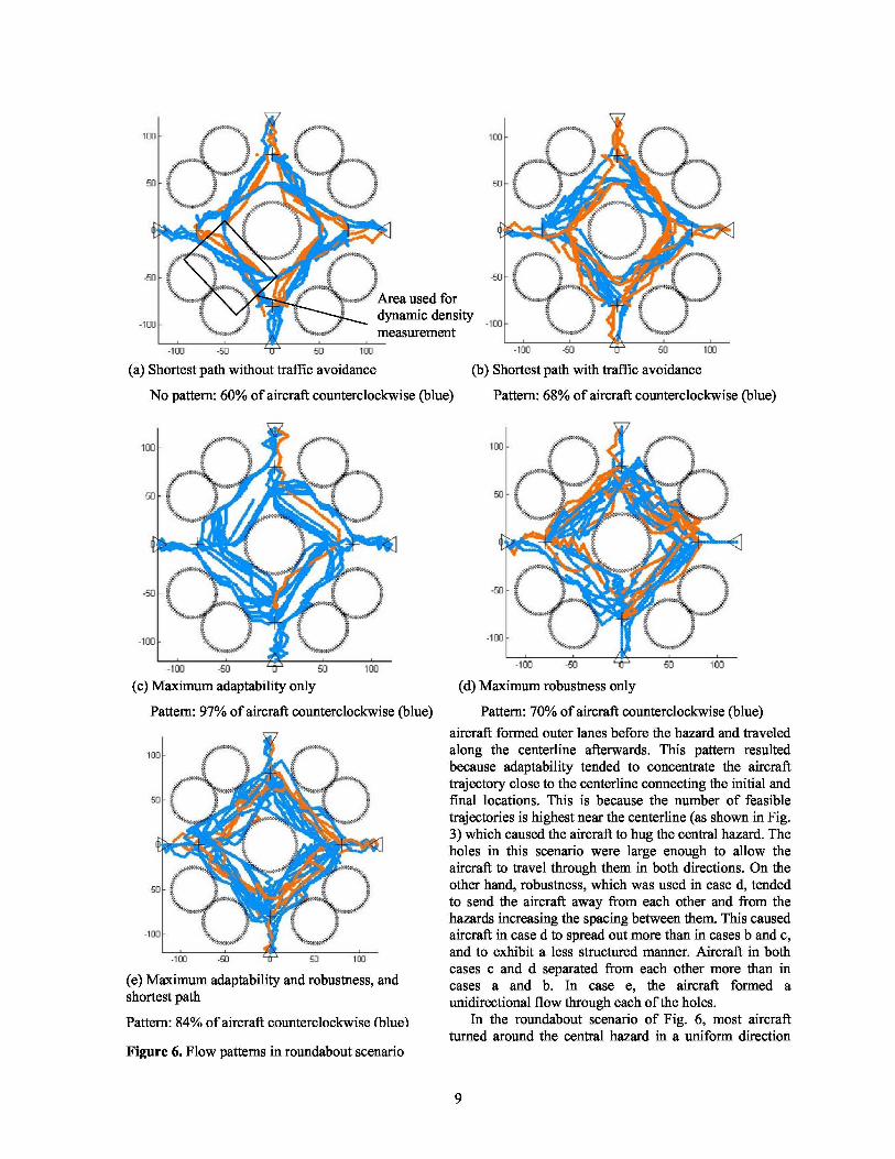
B. Results and ObservationsFig. 5 (a-e) demonstrate the resulting flow patterns in the first scenario and Fig. 6 (a-e) those in the second

scenario, using full trajectories. As a baseline the shortest path cost function was run twice, once without avoidingthe other traffic (cases a) and once with avoiding it (cases b). Traffic avoidance was turned off to depict currentpractice where conflict avoidance is only applied in a short time horizon of 10-20 minutes. Shortest-path with trafficavoidance sets another baseline for demonstrating the marginal effect of using the adaptability and robustnessmetrics instead. When using adaptability and robustness metrics (cases c-e) traffic is naturally avoided

7

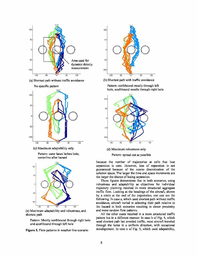
Pattern: outer lanes before hole,centerline after hazard

(e) Maximum adaptability and robustness, andshortest path

Pattern: Mostly northbound through right holeand southbound through left hole

Figure 5. Flow patterns in weather line scenario

Pattern: spread out as possible

because the number of trajectories at cells that loseseparation is zero. However, loss of separation is notguaranteed because of the coarse discretization of thesolution space. The larger the time and space increments arethe larger the chance of losing separation.

These figures demonstrate that in both scenarios, usingrobustness and adaptability as objectives for individualtrajectory planning resulted in more structured aggregatetraffic flow. Looking at the headings of the aircraft, shownby a circle at the end of the trajectories, one can see thefollowing. In case a, which used shortest path without trafficavoidance, aircraft varied in selecting their path relative tothe hazard in both scenarios resulting in closer proximityand more random flow patterns.

All the other cases resulted in a more structured trafficpattern but in a different manner: In case b of Fig. 5, whichused shortest path but avoided traffic, most aircraft traveledthrough the holes in a uniform direction, with occasionalmisalignment. In case c of Fig. 5, which used adaptability,

(a) Shortest path without traffic avoidance (b) Shortest path with traffic avoidance

ed forc densityement

No specific pattern

(c) Maximum adaptability only

Pattern: northbound mostly through lefthole, southbound mostly through right hole

(d) Maximum robustness only

ea used fornamic densityasurement

(a) Shortest path without traffic avoidance

(b) Shortest path with traffic avoidance

No pattern: 60% of aircraft counterclockwise (blue)

Pattern: 68% of aircraft counterclockwise (blue)

(d) Maximum robustness only(c) Maximum adaptability only

Pattern: 97% of aircraft counterclockwise (blue) Pattern: 70% of aircraft counterclockwise (blue)

(e) Maximum adaptability and robustness, andshortest path

Pattern: 84% of aircraft counterclockwise (blue)

Figure 6. Flow patterns in roundabout scenario

aircraft formed outer lanes before the hazard and traveledalong the centerline afterwards. This pattern resultedbecause adaptability tended to concentrate the aircrafttrajectory close to the centerline connecting the initial andfinal locations. This is because the number of feasibletrajectories is highest near the centerline (as shown in Fig.3) which caused the aircraft to hug the central hazard. Theholes in this scenario were large enough to allow theaircraft to travel through them in both directions. On theother hand, robustness, which was used in case d, tendedto send the aircraft away from each other and from thehazards increasing the spacing between them. This causedaircraft in case d to spread out more than in cases b and c,and to exhibit a less structured manner. Aircraft in bothcases c and d separated from each other more than incases a and b. In case e, the aircraft formed aunidirectional flow through each of the holes.

In the roundabout scenario of Fig. 6, most aircraftturned around the central hazard in a uniform direction

9

relative to the shortest path case a. This is indicated in the figure by the percentage of aircraft that selected thecounterclockwise direction (using the darker, blue color). This percentage is higher in cases c-e (70-97 percent) thancases a and b (60-68 percent).

The manner and degree to which the traffic self organizes depends on a number of factors. For example, thefollowing additional observations are made:

(1) cases e of Fig. 5 and 6 combine shortest path, adaptability and robustness in the cost function (12), with a =40 and b = 5000. These cases exhibited aspects from each of the b, c, and d cases: Because of robustness, aircraftspread out more. Because of adaptability, they formed a lane closer to the centerline especially after the hazard.Because of minimizing distance trajectories are smoother. The weights used in this example were not optimized andthe tradeoff between these factors is a subject of further research.

(2) The density of the traffic, a function of both the arrival rate and the size of the hazards, affects the pattern.For example, the aircraft managed to go through the holes in Fig. 5 in both directions.

(3) The first aircraft in the scenario does not encounter any traffic and hence makes random decisions if there areties between trajectories. The emerging traffic pattern depends on these early decisions. For the same reason, whentraffic density declines the pattern may switch to a new one.

(4) All aircraft in these scenarios used the same objective function. This induces implicit coordination and rulesand influences the emerging pattern.

(5) The shortest path case, with traffic avoidance (b) is closer to the adaptability case (c) than the robustness case(d). This is because the shortest path is close to the centerline where adaptability is high. The shortest pathtrajectory, however, differs from the most adaptable trajectory because it uses the minimum speed (to minimize pathstretching). Therefore these trajectories were smoother and exhibited less turns. Adaptable trajectories on the otherhand tended to zigzag around the centerline. Note that the jaggedness of the trajectories in all cases is an artifact ofthe low fidelity model used for this initial analysis to test the concept. Smoothness will be addressed and added infuture research while integrating the function with a higher fidelity trajectory generator.

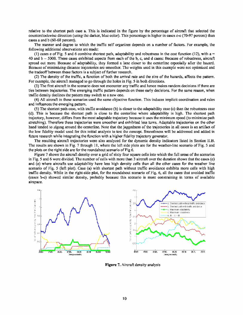
The resulting aircraft trajectories were also analyzed for the dynamic density indicators listed in Section II.B.The results are shown in Fig. 7 through 11, where the left side plots are for the weather-line scenario of Fig. 5 andthe plots on the right side are for the roundabout scenario of Fig 6.

Figure 7 shows the aircraft density over a grid of sixty four square cells into which the full areas of the scenariosin Fig. 5 and 6 were divided. The number of cells with more than 3 aircraft over the duration shows that the cases (c)and (e) where aircrafts use adaptability have less high density cells than all the other cases for the weather linescenario of Fig. 5 (left plot). Case (a) with shortest path without traffic avoidance exhibits more cells with hightraffic density. While in the right-side plot, for the roundabout scenario of Fig. 6, all the cases that avoided traffic(cases b-e) showed similar density, probably because this scenario is more constraining in terms of availableairspace.

Figure 7. Aircraft density analysis

10

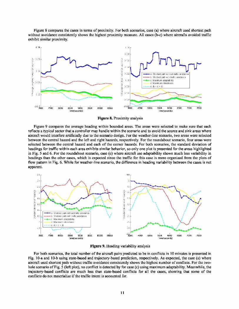
Figure 8 compares the cases in terms of proximity. For both scenarios, case (a) where aircraft used shortest pathwithout avoidance consistently shows the highest proximity measure. All cases (b-e) where aircrafts avoided trafficexhibit similar proximity.

Figure 8. Proximity analysis

Figure 9 compares the average heading within bounded areas. The areas were selected to make sure that eachreflects a typical sector that a controller may handle within the scenario and to avoid the source and sink areas whereaircraft would interfere artificially due to the scenario design. For the weather-line scenario, two areas were selectedbetween the central hazard and the left and right hazards, respectively. For the roundabout scenario, four areas wereselected between the central hazard and each of the corner hazards. For both scenarios, the standard deviation ofheadings for traffic within each area exhibits similar behavior, so only one plot is presented for the areas highlightedin Fig. 5 and 6. For the roundabout scenario, case (c) where aircraft use adaptability shows much less variability inheadings than the other cases, which is expected since the traffic for this case is more organized from the plots offlow pattern in Fig. 6. While for weather-line scenario, the difference in heading variability between the cases is notapparent.

Figure 9. Heading variability analysis

For both scenarios, the total number of the aircraft pairs predicted to be in conflicts in 10 minutes is presented inFig. 10-a and 10-b using state-based and trajectory-based prediction, respectively. As expected, the case (a) whereaircraft used shortest path without traffic avoidance consistently shows the highest number of conflicts. For the two-hole scenario of Fig. 5 (left plot), no conflict is detected by for case (c) using maximum adaptability. Meanwhile, thetrajectory-based conflicts are much less than state-based conflicts for all the cases, showing that some of theconflicts do not materialize if the traffic intent is accounted for.

11

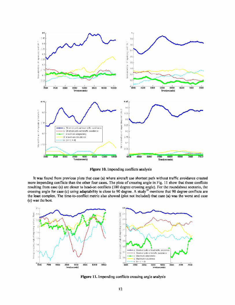
Figure 10. Impending conflicts analysis

It was found from previous plots that case (a) where aircraft use shortest path without traffic avoidance createdmore impending conflicts than the other four cases. The plots of crossing angle in Fig. 11 show that those conflictsresulting from case (a) are closer to head-on conflicts (180 degree crossing angle). For the roundabout scenario, thecrossing angle for case (c) using adaptability is close to 90 degree. A study 16 mentions that 90 degree conflicts arethe least complex. The time-to-conflict metric also showed (plot not included) that case (a) was the worst and case(c) was the best.

2 _ 2 s w,,

mot;.!'-,«r+

.....,w

z 4

w^1

/-iti^

_ 23' w

, ' ti t1 ^ ^

-^ 14

fft .{ r' ^L it [ e Si hates[ pQth vnihougtreFficl"ewidance

=^ ^I^lc ?i'r !b 1^;^ 1

7^ ___ ^b Sh0iL85[ p71h Yn1 F. Cr8ffi C18LOitl8t[B 1 i^F

i 1 ^ - J,.'r ;i^:. ^ ^^c Maximumladap[aGli^y.^ ^^^ ^ t ^ n n d. ilazimumlro6us[ness' - ^

Oa 151004 198p 8008 9999 9008 3904 Ipp10 10608 4000 494U 9008 5809 8000 9500 iC89 75Ktp

:nglsr[mg4 :rrWS*CM Y

Figure 11. Impending conflicts crossing angle analysis

12

V. Conclusions and Future ExtensionsThe analysis reported in this paper demonstrated that using adaptability and robustness metrics in planning

flexible aircraft trajectories results in traffic complexity mitigation. Two scenarios showed signs of self separationand self organization when using these metrics. The impact was quantified using dynamic density indicators. Theyindicated that using adaptability and robustness reduced aircraft density and the potential for conflict betweenaircraft. These flexibility metrics can be combined with other metrics in the trajectory planning of pilots, airlines,and traffic managers. By incorporating these metrics, the contribution of each aircraft to traffic complexity would bereduced, even without explicit coordination among aircraft or for the aircraft by a ground system.

The results reported in this paper are promising, and open the door for a wide range of future research. Suchresearch extension includes the investigation of: the sensitivity to varying a number of factors such as traffic densityand severity of constraints; the effect of dynamic and stochastic decision making where each aircraft updates itstrajectory plan over time in response to uncertainty; sensitivity to varying the cost function and the tradeoff betweenadaptability, robustness and other metrics of interest to users and traffic managers; the effect of non-uniform,competing cost functions among different aircraft; the impact of explicit rules and coordination on furthering selforganization; and the application of the metrics and algorithms presented in higher-fidelity real-time systems.

AcknowledgmentThis research was funded by NASA under contract NNA07BA86C.

References1 Joint Planning and Development Office, “Next Generation Air Transportation System Integrated Plan,” URL:

http://www.jpdo.gov/library/NGATS_v1_1204r.pdf.

2Wing, D., “A Potentially Useful Role for Airborne Separation in 4D-Trajectory ATM Operations,” Proceedingsof the 5th AIAA Aviation Technology Integration and Operations (ATIO) Conference, AIAA-2005-7336, 2005.

3Green, S. M., Bilimoria, K. D., and Ballin, M. G., “Distributed Air/Ground Traffic Management for En RouteFlight Operations.” Air Traffic Control Quarterly, Vol. 9, No. 4, 2001, pp. 259–285.

4Idris, H., Vivona, R., Penny, S., Krozel, J., and Bilimoria, K., “Operational Concept for Collaborative TrafficFlow Management based on Field Observations,” Proceedings of the 5th AIAA 5th Aviation Technology, Integrationand Operations (ATIO) Conference, AIAA-2005-7434, 2005.

5Krishnamurthy, K., Barmore, B., and Bussink, F., “Airborne Precision Spacing in Merging terminal ArrivalRoutes,” 6th USA/Europe Air Traffic Management R&D Seminar, 2005.

6Blom H.A.P., B. Klein Obbink, and G.I. Bakker, “Safety Risk Simulation of an Airborne Self SeparationConcept of Operation,” Proceedings of the 7th AIAA Aviation Technology Integration and Operations (ATIO)Conference, AIAA 2007-7729.

7Barhydt, R., and Kopardekar, P., “Joint NASA Ames/Langley Experimental Evaluation of IntegratedAir/Ground Operations for En Route Free maneuvering,” 6th USA/Europe Air Traffic Management R&D Seminar,2005.

8Mediterranean Free Flight Programme Final Report, D821, http://www.medff.it/public/index.asp, November2005.

9Erzberger, H., T.J. Davis, and S.M. Green, “Design of Center-TRACON Automation System,” AGARD Meetingon Machine Intelligence in ATM, Berlin, Germany, 1993.

10Idris H., D. Wing, R. Vivona, and J.L. Garcia-Chico, “A Distributed Trajectory-Oriented Approach toManaging Traffic Complexity,” Proceedings of the 7th AIAA Aviation Technology Integration and Operations(ATIO) Conference, AIAA-2007-7731, 2007.

11 Idris H., R. Vivona, J.L. Garcia-Chico, and D. Wing, “Distributed Traffic Complexity Management byPreserving Trajectory Flexibility,” Proceeding of the 26th Digital Avionics Systems Conference, 2007.

12Idris H, T. El-Wakil, and D. Wing, “Trajectory planning by preserving flexibility: metrics and analysis,”Proceedings of the AIAA Guidance Navigation and Control (GNC) Conference, AIAA-2008-7406, 2008.

13

13Idris H., and R. Vivona, “Metrics for Traffic Complexity Management in Self-Separation Operations,” AirTraffic Control Quarterly, Volume 17, Number 1, 2009.

14Laudeman, I.V., Shelden, S.G., Branstrom, R., & Brasil, C.L., 1999, Dynamic Density: An Air TrafficManagement Metric, NASA-TM-1998-112226

15 Sridhar, B., Sheth, K.S., & Grabbe, S., Airspace Complexity and its Application in Air Traffic Management,2nd USA/Europe Air Traffic Management R&D Seminar, Orlando, Florida

16 Chatterji, G. B. & Sridhar B., 2001, Measures for Air Traffic Controller Workload Prediction, Proceedings ofthe First AIAA Aircraft Technology, Integration, and Operations Forum, Los Angles, CA.

17Kopardekar. P. and S. Magyarits, “Measurements and prediction of dynamic density,” 5th USA/Europe ATMR&D Seminar, 2003.

18 Davison, J., Histon, J., Ragnarsdottir, M., Major, L., Hansman, R.J., "Impact of Operating Context on the Useof Structure in Air Traffic Controller Cognitive Processes". 5th USA/Europe Air Traffic Management R&D Seminar,2002.

19Delahaye, D. Puechmorel, S., Hansman, R.J., and Histon, J., “Air traffic complexity based on non lineardynamical systems”, 5th USA/Europe Air Traffic Management R&D Seminar, 2003.

20Idris H., D. Delahaye, and D. Wing, “Distributed Traffic Flexibility Preservation for Traffic ComplexityMitigation ,” 8th USA/Europe Air Traffic Management R&D Seminar, 2009.

21J. Krozel, T. Mueller, and G. Hunter, “Free flight conflict detection and resolution analysis,” Proceedings ofthe AIAA Guidance Navigation and Control (GNC) Conference, San Diego, CA, 1996.

14