analysis of the forecasting performance of the threshold
TRANSCRIPT

Analysis of the Forecasting Performance of the ThresholdAutoregressive Model
PAOLA ANDREA VACA GONZALEZ
ECONOMIST
UNIVERSIDAD NACIONAL DE COLOMBIA
FACULTY OF SCIENCE
STATISTICS DEPARTMENT
BOGOTA, D.C.
APRIL 2018
Analysis of the Forecasting Performance of the ThresholdAutoregressive Model
PAOLA ANDREA VACA GONZALEZ
ECONOMIST
THESIS PRESENTED FOR THE
MASTER IN STATISTICS SCIENCE DEGREE
ADVISOR
FABIO HUMBERTO NIETO SANCHEZ
DOCTOR IN STATISTICS
UNIVERSIDAD NACIONAL DE COLOMBIA
FACULTY OF SCIENCE
STATISTICS DEPARTMENT
BOGOTA, D.C.
APRIL 2018

Title
Analysis of the Forecasting Performance of the Threshold Autoregressive Model
Tıtulo
Analisis de la Capacidad de Pronostico del Modelo Autorregresivo de Umbrales
Abstract
In this investigation, we analyze the forecasting performance of the threshold autoregressi-
ve (TAR) model. To this aim, we find the Bayesian predictive distribution from this model,
and then, we conduct an out-of-sample forecasting exercise, where we compare forecasts
from the TAR model with those from a linear model and nonlinear smooth transition
autoregressive, self-exciting threshold autoregressive and Markov-switching autoregressive
models. For this empirical forecast evaluation, we: i) use the U.S. and Colombian GDP,
unemployment rate, industrial production index and inflation time series, which lead us
to estimate and forecast forty models; and, ii) use evaluation criteria and statistical tests
that are mostly employed in literature. We also compare the in-sample properties of the
estimated models. For the overall comparison, we find a satisfactory performance of the
TAR model in forecasting the chosen economic time series, and a shape changing charac-
teristic in the Bayesian predictive distributions of this model that may capture the cycles
in the economic time series. This gives important signals about the forecasting ability of
the TAR model in the economic field.
Resumen
En esta investigacion, se analiza la capacidad de pronostico del modelo Autorregresivo de
Umbrales (TAR). Para esta finalidad, se encuentra la distribucion predictiva Bayesiana,
y luego, se conduce un ejercicio de pronostico fuera de la muestra, donde se comparan
los pronosticos del modelo TAR con auqellos de un modelo lineal y de los modelos no
lineales Autorregresivo de Transicion Suave, Autorregresivo de Umbrales Auto-Excitado y
Autorregresivo de Cambio de Regimen. Para esta evaluacion de pronosticos empırica, i) se
utilizan las series del PIB, el desempleo, el ındice de produccion industrial y la inflacion de
Estados Unidos y Colombia, lo cual lleva a estimar y pronosticar cuarenta modelos; y, ii)
se utilizan criterios y test estadısticos los cuales on ampliamente aplicados en la literatura.
De igual manera, se comparan las propiedades dentro de la muestra de los modelos estima-
dos. Para todo el ejercicio de comparacion, se encuentra un comportamiento satisfactorio
del modelo TAR para pronosticar las distintas series economicas, y se encuentra una ca-
racterıstica de cambio de forma en la distribucion predictiva del modelo TAR que puede
capturar los ciclos presentados en las series economicas. Esto arroja importantes indicios
sobre la capacidad de pronostico del modelo TAR en el campo economico.
Keywords: Bayesian predictive distributions; Forecasts comparison; Threshold autoregressive mo-
del; Linear model; Nonlinear model.
Palabras clave: Distribuciones predictivas Bayesianas; Comparacion de pronosticos; Modelo au-
torregresivo de umbrales; modelo lineal; modelo no lineal.

To God and my Family for their endless love and support.

I thank Professor Fabio Nieto for his guidance and support, Professor Sergio Calderon
for his suggestions and the Universidad Nacional de Colombia for its support.

Contents
List of Tables IX
List of Figures XIV
Introduction XXI
1. Forecasting Models 1
1.1. Threshold autoregressive model . . . . . . . . . . . . . . . . . . . . . . . . . 1
1.1.1. Model estimation . . . . . . . . . . . . . . . . . . . . . . . . . . . . . 3
1.1.2. Forecasting procedure . . . . . . . . . . . . . . . . . . . . . . . . . . 4
1.2. Self-exciting threshold autoregressive model . . . . . . . . . . . . . . . . . . 6
1.2.1. Model estimation . . . . . . . . . . . . . . . . . . . . . . . . . . . . . 7
1.2.2. Forecasting procedure . . . . . . . . . . . . . . . . . . . . . . . . . . 7
1.3. Smooth transition autoregressive model . . . . . . . . . . . . . . . . . . . . 8
1.3.1. Model estimation . . . . . . . . . . . . . . . . . . . . . . . . . . . . . 9
1.3.2. Forecasting procedure . . . . . . . . . . . . . . . . . . . . . . . . . . 10
1.4. Markov-switching autoregressive model . . . . . . . . . . . . . . . . . . . . 10
1.4.1. Model estimation . . . . . . . . . . . . . . . . . . . . . . . . . . . . . 11
1.4.2. Forecasting procedure . . . . . . . . . . . . . . . . . . . . . . . . . . 11
1.5. Autoregressive model . . . . . . . . . . . . . . . . . . . . . . . . . . . . . . 12
1.5.1. Model estimation . . . . . . . . . . . . . . . . . . . . . . . . . . . . . 12
1.5.2. Forecasting procedure . . . . . . . . . . . . . . . . . . . . . . . . . . 13
2. Evaluation criteria 14
2.1. Unbiased forecasts . . . . . . . . . . . . . . . . . . . . . . . . . . . . . . . . 14
2.2. Uncorrelated forecasts . . . . . . . . . . . . . . . . . . . . . . . . . . . . . . 15
2.3. Relative mean square error . . . . . . . . . . . . . . . . . . . . . . . . . . . 15
2.4. Theil’s U statistic . . . . . . . . . . . . . . . . . . . . . . . . . . . . . . . . . 15
2.5. Diebold-Mariano test . . . . . . . . . . . . . . . . . . . . . . . . . . . . . . . 16
2.6. Forecast encompassing test . . . . . . . . . . . . . . . . . . . . . . . . . . . 17
2.7. Graphical analysis . . . . . . . . . . . . . . . . . . . . . . . . . . . . . . . . 18
3. Selection of the data 19
3.1. Unemployment rate . . . . . . . . . . . . . . . . . . . . . . . . . . . . . . . 19

Contents vii
3.2. Gross domestic product . . . . . . . . . . . . . . . . . . . . . . . . . . . . . 20
3.3. Industrial production index . . . . . . . . . . . . . . . . . . . . . . . . . . . 21
3.4. Inflation . . . . . . . . . . . . . . . . . . . . . . . . . . . . . . . . . . . . . . 21
4. Out-of-sample forecast evaluation 23
4.1. Empirical results for the United States economic time series . . . . . . . . . 24
4.1.1. Unemployment rate . . . . . . . . . . . . . . . . . . . . . . . . . . . 24
4.1.2. Gross domestic product . . . . . . . . . . . . . . . . . . . . . . . . . 38
4.1.3. Industrial production index . . . . . . . . . . . . . . . . . . . . . . . 44
4.1.4. Inflation . . . . . . . . . . . . . . . . . . . . . . . . . . . . . . . . . . 50
4.2. Empirical results for the Colombian economic time series . . . . . . . . . . 56
4.2.1. Unemployment rate . . . . . . . . . . . . . . . . . . . . . . . . . . . 56
4.2.2. Gross domestic product . . . . . . . . . . . . . . . . . . . . . . . . . 64
4.2.3. Industrial production index . . . . . . . . . . . . . . . . . . . . . . . 69
4.2.4. Inflation . . . . . . . . . . . . . . . . . . . . . . . . . . . . . . . . . . 75
Conclusions 83
A. Theoretical Background 84
A.1. Gibbs Sampler . . . . . . . . . . . . . . . . . . . . . . . . . . . . . . . . . . 84
A.2. Bayesian Predictive Distributions . . . . . . . . . . . . . . . . . . . . . . . . 85
B. General review of the models estimation for the change in the U.S. unem-
ployment rate 86
B.1. Estimation of the TAR model . . . . . . . . . . . . . . . . . . . . . . . . . . 86
B.2. Estimation of the SETAR model . . . . . . . . . . . . . . . . . . . . . . . . 90
B.3. Estimation of the STAR model . . . . . . . . . . . . . . . . . . . . . . . . . 91
B.4. Estimation of the MSAR model . . . . . . . . . . . . . . . . . . . . . . . . . 92
C. General review of the models estimation for the annual growth rate of the
U.S. real GDP 93
C.1. Estimation of the TAR model . . . . . . . . . . . . . . . . . . . . . . . . . . 93
C.2. Estimation of the SETAR model . . . . . . . . . . . . . . . . . . . . . . . . 99
C.3. Estimation of the STAR model . . . . . . . . . . . . . . . . . . . . . . . . . 101
C.4. Estimation of the MSAR model . . . . . . . . . . . . . . . . . . . . . . . . . 103
C.5. Estimation of the AR model . . . . . . . . . . . . . . . . . . . . . . . . . . . 104
D. General review of the models estimation for the annual growth rate of the
U.S. Industrial Production Index 106
D.1. Estimation of the TAR model . . . . . . . . . . . . . . . . . . . . . . . . . . 106
D.2. Estimation of the SETAR model . . . . . . . . . . . . . . . . . . . . . . . . 112
D.3. Estimation of the STAR model . . . . . . . . . . . . . . . . . . . . . . . . . 114
D.4. Estimation of the MSAR model . . . . . . . . . . . . . . . . . . . . . . . . . 115
D.5. Estimation of the AR model . . . . . . . . . . . . . . . . . . . . . . . . . . . 117

Contents viii
E. General review of the models estimation for the growth rate of the U.S.
quarterly CPI 119
E.1. Estimation of the TAR model . . . . . . . . . . . . . . . . . . . . . . . . . . 119
E.2. Estimation of the SETAR model . . . . . . . . . . . . . . . . . . . . . . . . 124
E.3. Estimation of the STAR model . . . . . . . . . . . . . . . . . . . . . . . . . 126
E.4. Estimation of the MSAR model . . . . . . . . . . . . . . . . . . . . . . . . . 128
E.5. Estimation of the AR model . . . . . . . . . . . . . . . . . . . . . . . . . . . 129
F. General review of the model estimation for the change in the Colombian
unemployment rate 131
F.1. Estimation of the TAR model . . . . . . . . . . . . . . . . . . . . . . . . . . 131
F.2. Estimation of the SETAR model . . . . . . . . . . . . . . . . . . . . . . . . 136
F.3. Estimation of the STAR model . . . . . . . . . . . . . . . . . . . . . . . . . 138
F.4. Estimation of the MSAR model . . . . . . . . . . . . . . . . . . . . . . . . . 140
F.5. Estimation of the AR model . . . . . . . . . . . . . . . . . . . . . . . . . . . 141
G. General review of the model estimation for the annual growth rate of the
Colombian GDP 143
G.1. Estimation of the TAR model . . . . . . . . . . . . . . . . . . . . . . . . . . 143
G.2. Estimation of the SETAR model . . . . . . . . . . . . . . . . . . . . . . . . 148
G.3. Estimation of the STAR model . . . . . . . . . . . . . . . . . . . . . . . . . 150
G.4. Estimation of the MSAR model . . . . . . . . . . . . . . . . . . . . . . . . . 151
G.5. Estimation of the AR model . . . . . . . . . . . . . . . . . . . . . . . . . . . 153
H. General review of the models estimation for the biannual growth rate of the
Colombian Industrial Production Index 155
H.1. Estimation of the TAR model . . . . . . . . . . . . . . . . . . . . . . . . . . 155
H.2. Estimation of the SETAR model . . . . . . . . . . . . . . . . . . . . . . . . 160
H.3. Estimation of the STAR model . . . . . . . . . . . . . . . . . . . . . . . . . 162
H.4. Estimation of the MSAR model . . . . . . . . . . . . . . . . . . . . . . . . . 164
H.5. Estimation of the AR model . . . . . . . . . . . . . . . . . . . . . . . . . . . 165
I. General review of the models estimation for the growth rate of the Colombian
CPI 167
I.1. Estimation of the TAR model . . . . . . . . . . . . . . . . . . . . . . . . . . 167
I.2. Estimation of the SETAR model . . . . . . . . . . . . . . . . . . . . . . . . 172
I.3. Estimation of the STAR model . . . . . . . . . . . . . . . . . . . . . . . . . 174
I.4. Estimation of the MSAR model . . . . . . . . . . . . . . . . . . . . . . . . . 175
I.5. Estimation of the AR model . . . . . . . . . . . . . . . . . . . . . . . . . . . 177
Bibliography 179

List of Tables
4.1. Model adequacy. U.S. unemployment rate case. . . . . . . . . . . . . . . . . 32
4.2. p–values of the (a) unbiased test and (b) correlation test for the first 4 lags.
U.S. unemployment rate case. . . . . . . . . . . . . . . . . . . . . . . . . . . 32
4.3. Relative MSE of forecasts. U.S. unemployment rate case. . . . . . . . . . . 33
4.4. DM test when (a) H1 : Forecasts from competing model (F2) are better
than forecasts from TAR model (F1) and (b) H1 : F1 are better than F2;
MDM test when (c) H1 : F2 are better than F1 and (d) H1 : F1 are better
than F2. U.S. unemployment rate case. . . . . . . . . . . . . . . . . . . . . 33
4.5. CH test when (a) H0 : F1 encompasses F2 and (b) H0: F2 encompasses F1;
ER test when (c) H0 : F1 encompasses F2 and (d) H0: F2 encompasses F1;
HLN test when (e) H0 : F1 encompasses F2 and (f) H0: F2 encompasses
F1. U.S. unemployment rate case. . . . . . . . . . . . . . . . . . . . . . . . 34
4.6. Theil’s U statistic. U.S. unemployment rate case. . . . . . . . . . . . . . . . 35
4.7. Summary of the forecasting performance of the TAR model. U.S. unem-
ployment rate case. . . . . . . . . . . . . . . . . . . . . . . . . . . . . . . . . 36
4.8. Model adequacy. U.S. GDP case. . . . . . . . . . . . . . . . . . . . . . . . . 39
4.9. p–values of the (a) unbiased test and (b) correlation test for the first 4 lags.
U.S. GDP case. . . . . . . . . . . . . . . . . . . . . . . . . . . . . . . . . . . 39
4.10. Relative MSE of forecasts. U.S. GDP case. . . . . . . . . . . . . . . . . . . 39
4.11. DM test when (a) H1 : Forecasts from competing model (F2) are better
than forecasts from TAR model (F1) and (b) H1 : F1 are better than F2;
MDM test when (c) H1 : F2 are better than F1 and (d) H1 : F1 are better
than F2. U.S. GDP case. . . . . . . . . . . . . . . . . . . . . . . . . . . . . 40
4.12. CH test when (a) H0 : F1 encompasses F2 and (b) H0: F2 encompasses F1;
ER test when (c) H0 : F1 encompasses F2 and (d) H0: F2 encompasses F1;
HLN test when (e) H0 : F1 encompasses F2 and (f) H0: F2 encompasses
F1. U.S. GDP case. . . . . . . . . . . . . . . . . . . . . . . . . . . . . . . . 41
4.13. Theil’s U statistic. U.S. GDP case. . . . . . . . . . . . . . . . . . . . . . . . 41
4.14. Summary of the forecasting performance of the TAR model. U.S. GDP case. 42
4.15. Model adequacy. U.S. indpro case. . . . . . . . . . . . . . . . . . . . . . . . 45
4.16. p–values of the (a) unbiased test and (b) correlation test for the first 4 lags.
U.S. indpro case. . . . . . . . . . . . . . . . . . . . . . . . . . . . . . . . . . 45

List of Tables x
4.17. Relative MSE of forecasts. U.S. indpro case. . . . . . . . . . . . . . . . . . . 45
4.18. DM test when (a) H1 : Forecasts from competing model (F2) are better
than forecasts from TAR model (F1) and (b) H1 : F1 are better than F2;
MDM test when (c) H1 : F2 are better than F1 and (d) H1 : F1 are better
than F2. U.S. indpro case. . . . . . . . . . . . . . . . . . . . . . . . . . . . . 46
4.19. CH test when (a) H0 : F1 encompasses F2 and (b) H0: F2 encompasses F1;
ER test when (c) H0 : F1 encompasses F2 and (d) H0: F2 encompasses F1;
HLN test when (e) H0 : F1 encompasses F2 and (f) H0: F2 encompasses
F1. U.S. indpro case. . . . . . . . . . . . . . . . . . . . . . . . . . . . . . . . 47
4.20. Theil’s U statistic. U.S. indpro case. . . . . . . . . . . . . . . . . . . . . . . 47
4.21. Summary of the forecasting performance of the TAR model. U.S. indpro case. 48
4.22. Model adequacy. U.S. CPI case. . . . . . . . . . . . . . . . . . . . . . . . . 51
4.23. p–values of the (a) unbiased test and (b) correlation test for the first 4 lags.
U.S. CPI case. . . . . . . . . . . . . . . . . . . . . . . . . . . . . . . . . . . 51
4.24. Relative MSE of forecasts. U.S. CPI case. . . . . . . . . . . . . . . . . . . . 52
4.25. DM test when (a) H1 : Forecasts from competing model (F2) are better
than forecasts from TAR model (F1) and (b) H1 : F1 are better than F2;
MDM test when (c) H1 : F2 are better than F1 and (d) H1 : F1 are better
than F2. U.S. CPI case. . . . . . . . . . . . . . . . . . . . . . . . . . . . . . 52
4.26. CH test when (a) H0 : F1 encompasses F2 and (b) H0: F2 encompasses F1;
ER test when (c) H0 : F1 encompasses F2 and (d) H0: F2 encompasses F1;
HLN test when (e) H0 : F1 encompasses F2 and (f) H0: F2 encompasses
F1. U.S. CPI case. . . . . . . . . . . . . . . . . . . . . . . . . . . . . . . . . 53
4.27. Theil’s U statistic. U.S. CPI case. . . . . . . . . . . . . . . . . . . . . . . . 53
4.28. Summary of the forecasting performance of the TAR model. U.S. CPI case 54
4.29. Model adequacy. Colombian unemployment rate case. . . . . . . . . . . . . 57
4.30. p–values of the (a) unbiased test and (b) correlation test for the first 4 lags.
Colombian unemployment rate case. . . . . . . . . . . . . . . . . . . . . . . 58
4.31. Relative MSE of forecasts. Colombian unemployment rate case. . . . . . . . 58
4.32. DM test when (a) H1 : Forecasts from competing model (F2) are better
than forecasts from TAR model (F1) and (b) H1 : F1 are better than F2;
MDM test when (c) H1 : F2 are better than F1 and (d) H1 : F1 are better
than F2. Colombian unemployment rate case. . . . . . . . . . . . . . . . . . 59
4.33. CH test when (a) H0 : F1 encompasses F2 and (b) H0: F2 encompasses F1;
ER test when (c) H0 : F1 encompasses F2 and (d) H0: F2 encompasses F1;
HLN test when (e) H0 : F1 encompasses F2 and (f) H0: F2 encompasses
F1. Colombian unemployment rate case. . . . . . . . . . . . . . . . . . . . . 60
4.34. Theil’s U statistic. Colombian unemployment rate case. . . . . . . . . . . . 61
4.35. Summary of the forecasting performance of the TAR model. Colombian
unemployment rate case. . . . . . . . . . . . . . . . . . . . . . . . . . . . . . 62
4.36. Model adequacy. Colombian GDP case. . . . . . . . . . . . . . . . . . . . . 65
4.37. p–values of the (a) unbiased test and (b) correlation test for the first 4 lags.
Colombian GDP case. . . . . . . . . . . . . . . . . . . . . . . . . . . . . . . 65
4.38. Relative MSE of forecasts. Colombian GDP case. . . . . . . . . . . . . . . . 66

List of Tables xi
4.39. DM test when (a) H1 : Forecasts from competing model (F2) are better
than forecasts from TAR model (F1) and (b) H1 : F1 are better than F2;
MDM test when (c) H1 : F2 are better than F1 and (d) H1 : F1 are better
than F2. Colombian GDP case. . . . . . . . . . . . . . . . . . . . . . . . . . 66
4.40. CH test when (a) H0 : F1 encompasses F2 and (b) H0: F2 encompasses F1;
ER test when (c) H0 : F1 encompasses F2 and (d) H0: F2 encompasses F1;
HLN test when (e) H0 : F1 encompasses F2 and (f) H0: F2 encompasses
F1. Colombian GDP case. . . . . . . . . . . . . . . . . . . . . . . . . . . . . 67
4.41. Theil’s U statistic. Colombian GDP case. . . . . . . . . . . . . . . . . . . . 68
4.42. Summary of the forecasting performance of the TAR model. Colombian
GDP case. . . . . . . . . . . . . . . . . . . . . . . . . . . . . . . . . . . . . . 69
4.43. Model adequacy. Colombian indpro case. . . . . . . . . . . . . . . . . . . . 70
4.44. p–values of the (a) unbiased test and (b) correlation test for the first 4 lags.
Colombian indpro case. . . . . . . . . . . . . . . . . . . . . . . . . . . . . . 71
4.45. Relative MSE of forecasts. Colombian indpro case. . . . . . . . . . . . . . . 71
4.46. DM test when (a) H1 : Forecasts from competing model (F2) are better
than forecasts from TAR model (F1) and (b) H1 : F1 are better than F2;
MDM test when (c) H1 : F2 are better than F1 and (d) H1 : F1 are better
than F2. Colombian indpro case. . . . . . . . . . . . . . . . . . . . . . . . . 72
4.47. CH test when (a) H0 : F1 encompasses F2 and (b) H0: F2 encompasses F1;
ER test when (c) H0 : F1 encompasses F2 and (d) H0: F2 encompasses F1;
HLN test when (e) H0 : F1 encompasses F2 and (f) H0: F2 encompasses
F1. Colombian indpro case. . . . . . . . . . . . . . . . . . . . . . . . . . . . 73
4.48. Theil’s U statistic. Colombian indpro case. . . . . . . . . . . . . . . . . . . 74
4.49. Summary of the forecasting performance of the TAR model. Colombian
indpro case. . . . . . . . . . . . . . . . . . . . . . . . . . . . . . . . . . . . . 75
4.50. Model adequacy. Colombian CPI case. . . . . . . . . . . . . . . . . . . . . . 76
4.51. p–values of the (a) unbiased test and (b) correlation test for the first 4 lags.
Colombian CPI case. . . . . . . . . . . . . . . . . . . . . . . . . . . . . . . . 77
4.52. Relative MSE of forecasts. Colombian CPI case. . . . . . . . . . . . . . . . 77
4.53. DM test when (a) H1 : Forecasts from competing model (F2) are better
than forecasts from TAR model (F1) and (b) H1 : F1 are better than F2;
MDM test when (c) H1 : F2 are better than F1 and (d) H1 : F1 are better
than F2. Colombian CPI case. . . . . . . . . . . . . . . . . . . . . . . . . . 78
4.54. CH test when (a) H0 : F1 encompasses F2 and (b) H0: F2 encompasses F1;
ER test when (c) H0 : F1 encompasses F2 and (d) H0: F2 encompasses F1;
HLN test when (e) H0 : F1 encompasses F2 and (f) H0: F2 encompasses
F1. Colombian CPI case. . . . . . . . . . . . . . . . . . . . . . . . . . . . . 79
4.55. Theil’s U statistic. Colombian CPI case. . . . . . . . . . . . . . . . . . . . . 80
4.56. Summary of the forecasting performance of the TAR model. Colombian
CPI case. . . . . . . . . . . . . . . . . . . . . . . . . . . . . . . . . . . . . . 81
B.1. Set of possible number of regimes for the real data. U.S. unemployment rate
case. . . . . . . . . . . . . . . . . . . . . . . . . . . . . . . . . . . . . . . . . 88

List of Tables xii
B.2. Posterior probability function for the number of regimes for the real data.
U.S. unemployment rate case. . . . . . . . . . . . . . . . . . . . . . . . . . . 89
B.3. Posterior probabilities for the autoregressive orders in the real data. U.S.
unemployment rate case. . . . . . . . . . . . . . . . . . . . . . . . . . . . . . 89
B.4. Parameter estimates for the TAR model. U.S. unemployment rate case. . . 90
B.5. Parameter estimates for the SETAR model. U.S. unemployment rate case. . 91
B.6. Parameter estimates for the STAR model. U.S. unemployment rate case. . . 92
B.7. Parameter estimates for the MSAR model. U.S. unemployment rate case. . 92
C.1. Set of possible number of regimes for the real data. U.S. GDP case. . . . . 95
C.2. Posterior probability function for the number of regimes for the real data.
U.S. GDP case. . . . . . . . . . . . . . . . . . . . . . . . . . . . . . . . . . . 96
C.3. Posterior probabilities for the autoregressive orders in the real data. U.S.
GDP case. . . . . . . . . . . . . . . . . . . . . . . . . . . . . . . . . . . . . . 96
C.4. Parameter estimates for the TAR model. U.S. GDP case. . . . . . . . . . . 97
C.5. Parameter estimates for the SETAR model. U.S. GDP case. . . . . . . . . . 100
C.6. Parameter estimates for the STAR model. U.S. GDP case. . . . . . . . . . . 102
C.7. Parameter estimates for the MSAR model. U.S. GDP case. . . . . . . . . . 103
D.1. Set of possible number of regimes for the real data. U.S. indpro case. . . . . 108
D.2. Posterior probability function for the number of regimes for the real data.
U.S. indpro case. . . . . . . . . . . . . . . . . . . . . . . . . . . . . . . . . . 109
D.3. Posterior probabilities for the autoregressive orders in the real data. U.S.
indpro case. . . . . . . . . . . . . . . . . . . . . . . . . . . . . . . . . . . . . 109
D.4. Parameter estimates for the TAR model. U.S. indpro case. . . . . . . . . . 110
D.5. Parameter estimates for the SETAR model. U.S. indpro case. . . . . . . . . 113
D.6. Parameter estimates for the STAR model. U.S. indpro case. . . . . . . . . . 114
D.7. Parameter estimates for the MSAR model. U.S. indpro case. . . . . . . . . 116
E.1. Set of possible number of regimes for the real data. U.S. CPI case. . . . . . 121
E.2. Posterior probability function for the number of regimes for the real data.
U.S. CPI case. . . . . . . . . . . . . . . . . . . . . . . . . . . . . . . . . . . 121
E.3. Posterior probabilities for the autoregressive orders in the real data. U.S.
CPI case. . . . . . . . . . . . . . . . . . . . . . . . . . . . . . . . . . . . . . 122
E.4. Parameter estimates for the TAR model. U.S. CPI case. . . . . . . . . . . . 123
E.5. Parameter estimates for the SETAR model. U.S. CPI case. . . . . . . . . . 125
E.6. Parameter estimates for the STAR model. U.S. CPI case. . . . . . . . . . . 127
E.7. Parameter estimates for the MSAR model. U.S. CPI case. . . . . . . . . . . 128
F.1. Set of possible number of regimes for the real data. Colombian unemploy-
ment rate case. . . . . . . . . . . . . . . . . . . . . . . . . . . . . . . . . . . 133
F.2. Posterior probability function for the number of regimes for the real data.
Colombian unemployment rate case. . . . . . . . . . . . . . . . . . . . . . . 134
F.3. Posterior probabilities for the autoregressive orders in the real data. Colom-
bian unemployment rate case. . . . . . . . . . . . . . . . . . . . . . . . . . . 134
F.4. Parameter estimates for the TAR model. Colombian unemployment rate case.135

List of Tables xiii
F.5. Parameter estimates for the SETAR model. Colombian unemployment rate
case. . . . . . . . . . . . . . . . . . . . . . . . . . . . . . . . . . . . . . . . . 137
F.6. Parameter estimates for the STAR model. Colombian unemployment rate
case. . . . . . . . . . . . . . . . . . . . . . . . . . . . . . . . . . . . . . . . . 139
F.7. Parameter estimates for the MSAR model. Colombian unemployment rate
case. . . . . . . . . . . . . . . . . . . . . . . . . . . . . . . . . . . . . . . . . 140
G.1. Set of possible number of regimes for the real data. Colombian GDP case. . 145
G.2. Posterior probability function for the number of regimes for the real data.
Colombian GDP case. . . . . . . . . . . . . . . . . . . . . . . . . . . . . . . 146
G.3. Posterior probabilities for the autoregressive orders in the real data. Colom-
bian GDP case. . . . . . . . . . . . . . . . . . . . . . . . . . . . . . . . . . . 146
G.4. Parameter estimates for the TAR model. Colombian GDP case. . . . . . . . 147
G.5. Parameter estimates for the SETAR model. Colombian GDP case. . . . . . 149
G.6. Parameter estimates for the STAR model. Colombian GDP case. . . . . . . 150
G.7. Parameter estimates for the MSAR model. Colombian GDP case. . . . . . . 152
H.1. Set of possible number of regimes for the real data. Colombian indpro case. 157
H.2. Posterior probability function for the number of regimes for the real data.
Colombian indpro case. . . . . . . . . . . . . . . . . . . . . . . . . . . . . . 158
H.3. Posterior probabilities for the autoregressive orders in the real data. Colom-
bian indpro case. . . . . . . . . . . . . . . . . . . . . . . . . . . . . . . . . . 158
H.4. Parameter estimates for the TAR model. Colombian indpro case. . . . . . . 159
H.5. Parameter estimates for the SETAR model. Colombian indpro case. . . . . 161
H.6. Parameter estimates for the STAR model. Colombian indpro case. . . . . . 163
H.7. Parameter estimates for the MSAR model. Colombian indpro case. . . . . . 164
I.1. Set of possible number of regimes for the real data. Colombian CPI case. . 169
I.2. Posterior probability function for the number of regimes for the real data.
Colombian CPI case. . . . . . . . . . . . . . . . . . . . . . . . . . . . . . . . 170
I.3. Posterior probabilities for the autoregressive orders in the real data. Colom-
bian CPI case. . . . . . . . . . . . . . . . . . . . . . . . . . . . . . . . . . . 170
I.4. Parameter estimates for the TAR model. Colombian CPI case. . . . . . . . 171
I.5. Parameter estimates for the SETAR model. Colombian CPI case. . . . . . . 173
I.6. Parameter estimates for the STAR model. Colombian CPI case. . . . . . . 174
I.7. Parameter estimates for the MSAR model. Colombian CPI case. . . . . . . 176

List of Figures
4.1. (a) Time plot of the change in the U.S. quarterly unemployment rate and
(b) time plot of the growth rate of U.S. quarterly real GDP. . . . . . . . . . 25
4.2. Partial autocorrelation function of the fitted TAR model. (a) Standardized
residuals and (b) squared standardized residuals. U.S. unemployment rate
case. . . . . . . . . . . . . . . . . . . . . . . . . . . . . . . . . . . . . . . . . 26
4.3. (a) CUSUM and (b) CUSUMSQ charts for the residuals of the fitted TAR
model. U.S. unemployment rate case. . . . . . . . . . . . . . . . . . . . . . 27
4.4. Partial autocorrelation function of the fitted SETAR model. (a) Standard-
ized residuals and (b) squared standardized residuals. U.S. unemployment
rate case. . . . . . . . . . . . . . . . . . . . . . . . . . . . . . . . . . . . . . 28
4.5. (a) CUSUM and (b) CUSUMSQ charts for the residuals of the fitted SETAR
model. U.S. unemployment rate case. . . . . . . . . . . . . . . . . . . . . . 28
4.6. Partial autocorrelation function of the fitted STAR model. (a) Standardized
residuals and (b) squared standardized residuals. U.S. unemployment rate
case. . . . . . . . . . . . . . . . . . . . . . . . . . . . . . . . . . . . . . . . . 29
4.7. (a) CUSUM and (b) CUSUMSQ charts for the residuals of the fitted STAR
model. U.S. unemployment rate case. . . . . . . . . . . . . . . . . . . . . . 29
4.8. Partial autocorrelation function of the fitted MSAR model. (a) Standardized
residuals and (b) squared standardized residuals. U.S. unemployment rate
case. . . . . . . . . . . . . . . . . . . . . . . . . . . . . . . . . . . . . . . . . 30
4.9. (a) CUSUM and (b) CUSUMSQ charts for the residuals of the fitted MSAR
model. U.S. unemployment rate case. . . . . . . . . . . . . . . . . . . . . . 30
4.10. Partial autocorrelation function of the fitted AR model. (a) Standardized
residuals and (b) squared standardized residuals. U.S. unemployment rate
case. . . . . . . . . . . . . . . . . . . . . . . . . . . . . . . . . . . . . . . . . 31
4.11. (a) CUSUM and (b) CUSUMSQ charts for the residuals of the fitted AR
model. U.S. unemployment rate case. . . . . . . . . . . . . . . . . . . . . . 31
4.12. 1 to 8-step predictive distributions of the change in the unemployment rate
series, for the (a) TAR, (b) SETAR and (c) STAR models. U.S. unemploy-
ment rate case. . . . . . . . . . . . . . . . . . . . . . . . . . . . . . . . . . . 37
4.13. (a) Time plot of the annual growth rate of U.S. real GDP and (b) time plot
of U.S. term spread. . . . . . . . . . . . . . . . . . . . . . . . . . . . . . . . 38

List of Figures xv
4.14. 1 to 8-step predictive distributions of the annual growth rate of the U.S. real
output, for the (a) TAR, (b) SETAR and (c) STAR models. U.S. GDP case. 43
4.15. (a) Time plot of the annual growth rate of U.S. quarterly industrial produc-
tion index and (b) time plot of U.S. term spread. . . . . . . . . . . . . . . . 44
4.16. 1 to 8-step predictive distributions of the change in the unemployment rate
series, for the (a) TAR, (b) SETAR and (c) STAR models. U.S. indpro case. 49
4.17. (a) Time plot of the growth rate of U.S. quarterly CPI and (b) time plot of
U.S. term spread. . . . . . . . . . . . . . . . . . . . . . . . . . . . . . . . . . 50
4.18. 1 to 8-step predictive distributions of the change in the unemployment rate
series, for the (a) TAR, (b) SETAR and (c) STAR models. U.S. CPI case. . 55
4.19. (a) Time plot of the change in the the Colombian monthly unemployment
rate and (b) time plot of growth rate of Colombian ISE monthly index. . . 57
4.20. 1 to 8-step predictive distributions of the change in the unemployment rate
series, for the (a) TAR, (b) SETAR and (c) STAR models. Colombian
unemployment rate case. . . . . . . . . . . . . . . . . . . . . . . . . . . . . . 63
4.21. (a) Time plot of the annual growth rate of Colombian GDP and (b) time
plot of Colombian term spread. . . . . . . . . . . . . . . . . . . . . . . . . 64
4.22. (a) Time plot of the biannual growth rate of Colombian industrial production
index and (b) time plot of Colombian term spread. . . . . . . . . . . . . . . 70
4.23. (a) Time plot of the monthly growth rate of Colombian CPI and (b) time
plot of Colombian term spread. . . . . . . . . . . . . . . . . . . . . . . . . . 76
B.1. (a) Sample autocorrelation function and (b) sample partial autocorrelation
function for the change in the U.S. unemployment rate. . . . . . . . . . . . 86
B.2. (a) Sample autocorrelation function and (b) sample partial autocorrelation
function for the growth rate of U.S. real GDP. . . . . . . . . . . . . . . . . . 87
B.3. (a) Time plot of the change in the U.S. quarterly unemployment rate and
(b) Time plot of the growth rate of U.S. quarterly real GDP. . . . . . . . . 87
B.4. Nonparametric regression between the change in the U.S. unemployment
rate (X) and the growth rate of U.S. real GDP (Z). . . . . . . . . . . . . . . 88
B.5. Time plot of t-ratio of recursive estimates of the AR-3 coefficient in an ar-
ranged autoregression of order 3 and delay parameter 6. U.S. unemployment
rate case. . . . . . . . . . . . . . . . . . . . . . . . . . . . . . . . . . . . . . 91
C.1. (a) Sample autocorrelation function and (b) sample partial autocorrelation
function for the annual growth rate of U.S. real GDP. . . . . . . . . . . . . 93
C.2. (a) Sample autocorrelation function and (b) sample partial autocorrelation
function for the U.S. spread term. . . . . . . . . . . . . . . . . . . . . . . . 94
C.3. (a) Time plot of the annual growth rate of U.S. real GDP and (b) Time plot
of U.S. spread term. . . . . . . . . . . . . . . . . . . . . . . . . . . . . . . . 94
C.4. Nonparametric regression between the growth rate of U.S. real GDP (X)
and U.S. spread term (Z). . . . . . . . . . . . . . . . . . . . . . . . . . . . . 95
C.5. Partial autocorrelation function of the fitted TAR model. (a) Standardized
residuals and (b) squared standardized residuals. U.S. GDP case. . . . . . . 99

List of Figures xvi
C.6. (a) CUSUM and (b) CUSUMSQ charts for the residuals of the fitted TAR
model. U.S. GDP case. . . . . . . . . . . . . . . . . . . . . . . . . . . . . . . 99
C.7. Time plot of t-ratio of recursive estimates of the AR-2 coefficient in an
arranged autoregression of order 5 and delay parameter 2. U.S. GDP case. . 100
C.8. Partial autocorrelation function of the fitted SETAR model. (a) Standard-
ized residuals and (b) squared standardized residuals. U.S. GDP case. . . . 101
C.9. (a) CUSUM and (b) CUSUMSQ charts for the residuals of the fitted SETAR
model. U.S. GDP case. . . . . . . . . . . . . . . . . . . . . . . . . . . . . . . 101
C.10.Partial autocorrelation function of the fitted STAR model. (a) Standardized
residuals and (b) squared standardized residuals. U.S. GDP case. . . . . . . 102
C.11.(a) CUSUM and (b) CUSUMSQ charts for the residuals of the fitted STAR
model. U.S. GDP case. . . . . . . . . . . . . . . . . . . . . . . . . . . . . . . 103
C.12.Partial autocorrelation function of the fitted MSAR model. (a) Standardized
residuals and (b) squared standardized residuals. U.S. GDP case. . . . . . . 104
C.13.(a) CUSUM and (b) CUSUMSQ charts for the residuals of the fitted MSAR
model. U.S. GDP case. . . . . . . . . . . . . . . . . . . . . . . . . . . . . . . 104
C.14.Partial autocorrelation function of the fitted AR model. (a) Standardized
residuals and (b) squared standardized residuals. U.S. GDP case. . . . . . . 105
C.15.(a) CUSUM and (b) CUSUMSQ charts for the residuals of the fitted AR
model. U.S. GDP case. . . . . . . . . . . . . . . . . . . . . . . . . . . . . . . 105
D.1. (a) Sample autocorrelation function and (b) sample partial autocorrelation
function for the annual growth rate of U.S. industrial production index. . . 106
D.2. (a) Sample autocorrelation function and (b) sample partial autocorrelation
function for the U.S. spread term. . . . . . . . . . . . . . . . . . . . . . . . 107
D.3. (a) Time plot of the annual growth rate of U.S. industrial production index
and (b) Time plot of U.S. spread term. . . . . . . . . . . . . . . . . . . . . . 107
D.4. Nonparametric regression between the annual growth rate of the U.S. in-
dustrial production index (X) and U.S. spread term (Z). . . . . . . . . . . . 108
D.5. Partial autocorrelation function of the fitted TAR model. (a) Standardized
residuals and (b) squared standardized residuals. U.S. indpro case. . . . . . 111
D.6. (a) CUSUM and (b) CUSUMSQ charts for the residuals of the fitted TAR
model. U.S. indpro case. . . . . . . . . . . . . . . . . . . . . . . . . . . . . . 112
D.7. Time plot of t-ratio of recursive estimates of the AR-5 coefficient in an
arranged autoregression of order 9 and delay parameter 5. U.S. indpro case. 112
D.8. Partial autocorrelation function of the fitted SETAR model. (a) Standard-
ized residuals and (b) squared standardized residuals. U.S. indpro case. . . 113
D.9. (a) CUSUM and (b) CUSUMSQ charts for the residuals of the fitted SETAR
model. U.S. indpro case. . . . . . . . . . . . . . . . . . . . . . . . . . . . . . 114
D.10.Partial autocorrelation function of the fitted STAR model. (a) Standardized
residuals and (b) squared standardized residuals. U.S. indpro case. . . . . . 115
D.11.(a) CUSUM and (b) CUSUMSQ charts for the residuals of the fitted STAR
model. U.S. indpro case. . . . . . . . . . . . . . . . . . . . . . . . . . . . . . 115
D.12.Partial autocorrelation function of the fitted MSAR model. (a) Standardized
residuals and (b) squared standardized residuals. U.S. indpro case. . . . . . 116
List of Figures xvii
D.13.(a) CUSUM and (b) CUSUMSQ charts for the residuals of the fitted MSAR
model. U.S. indpro case. . . . . . . . . . . . . . . . . . . . . . . . . . . . . . 117
D.14.Partial autocorrelation function of the fitted AR model. (a) Standardized
residuals and (b) squared standardized residuals. U.S. indpro case. . . . . . 117
D.15.(a) CUSUM and (b) CUSUMSQ charts for the residuals of the fitted AR
model. U.S. indpro case. . . . . . . . . . . . . . . . . . . . . . . . . . . . . . 118
E.1. (a) Sample autocorrelation function and (b) sample partial autocorrelation
function for the growth rate of U.S. CPI. . . . . . . . . . . . . . . . . . . . . 119
E.2. (a) Sample autocorrelation function and (b) sample partial autocorrelation
function for the U.S. spread term. . . . . . . . . . . . . . . . . . . . . . . . 120
E.3. (a) Time plot of the annual growth rate of U.S. CPI and (b) Time plot of
U.S. spread term. . . . . . . . . . . . . . . . . . . . . . . . . . . . . . . . . . 120
E.4. Nonparametric regression between the growth rate of U.S. CPI (X) and the
U.S. spread term (Z). . . . . . . . . . . . . . . . . . . . . . . . . . . . . . . 121
E.5. Partial autocorrelation function of the fitted TAR model. (a) Standardized
residuals and (b) squared standardized residuals. U.S. CPI case. . . . . . . 124
E.6. (a) CUSUM and (b) CUSUMSQ charts for the residuals of the fitted TAR
model. U.S. CPI case. . . . . . . . . . . . . . . . . . . . . . . . . . . . . . . 124
E.7. Time plot of t-ratio of recursive estimates of the AR-9 coefficient in an
arranged autoregression of order 9 and delay parameter 2. U.S. CPI case. . 125
E.8. Partial autocorrelation function of the fitted SETAR model. (a) Standard-
ized residuals and (b) squared standardized residuals. U.S. CPI case. . . . . 126
E.9. (a) CUSUM and (b) CUSUMSQ charts for the residuals of the fitted SETAR
model. U.S. CPI case. . . . . . . . . . . . . . . . . . . . . . . . . . . . . . . 126
E.10.Partial autocorrelation function of the fitted STAR model. (a) Standardized
residuals and (b) squared standardized residuals. U.S. CPI case. . . . . . . 127
E.11.(a) CUSUM and (b) CUSUMSQ charts for the residuals of the fitted STAR
model. U.S. CPI case. . . . . . . . . . . . . . . . . . . . . . . . . . . . . . . 128
E.12.Partial autocorrelation function of the fitted MSAR model. (a) Standardized
residuals and (b) squared standardized residuals. U.S. CPI case. . . . . . . 129
E.13.(a) CUSUM and (b) CUSUMSQ charts for the residuals of the fitted MSAR
model. U.S. CPI case. . . . . . . . . . . . . . . . . . . . . . . . . . . . . . . 129
E.14.Partial autocorrelation function of the fitted AR model. (a) Standardized
residuals and (b) squared standardized residuals. U.S. CPI case. . . . . . . 130
E.15.(a) CUSUM and (b) CUSUMSQ charts for the residuals of the fitted AR
model. U.S. CPI case. . . . . . . . . . . . . . . . . . . . . . . . . . . . . . . 130
F.1. (a) Autocorrelation function and (b) partial autocorrelation function for
change in the Colombian unemployment rate. . . . . . . . . . . . . . . . . . 131
F.2. (a) Autocorrelation function and (b) partial autocorrelation function for the
growth rate of Colombian ISE index. . . . . . . . . . . . . . . . . . . . . . . 132
F.3. Growth rate of Colombian ISE index lagged 2 months and change in the
Colombian unemployment rate. . . . . . . . . . . . . . . . . . . . . . . . . . 132

List of Figures xviii
F.4. Nonparametric regression between the change in the Colombian unemploy-
ment rate (X) and the growth rate of Colombian ISE index (Z). . . . . . . . 133
F.5. Partial autocorrelation function of the fitted TAR model. (a) Standardized
residuals and (b) squared standardized residuals. Colombian unemployment
rate case. . . . . . . . . . . . . . . . . . . . . . . . . . . . . . . . . . . . . . 136
F.6. (a) CUSUM and (b) CUSUMSQ charts for the residuals of the fitted TAR
model. Colombian unemployment rate case. . . . . . . . . . . . . . . . . . . 136
F.7. Time plot of t-ratio of recursive estimates of the AR-2 coefficient in an
arranged autoregression of order 2 and delay parameter 2. Colombian un-
employment rate case. . . . . . . . . . . . . . . . . . . . . . . . . . . . . . . 137
F.8. Partial autocorrelation function of the fitted SETAR model. (a) Standard-
ized residuals and (b) squared standardized residuals. Colombian unem-
ployment rate case. . . . . . . . . . . . . . . . . . . . . . . . . . . . . . . . . 138
F.9. (a) CUSUM and (b) CUSUMSQ charts for the residuals of the fitted SETAR
model. Colombian unemployment rate case. . . . . . . . . . . . . . . . . . . 138
F.10.Partial autocorrelation function of the fitted STAR model. (a) Standardized
residuals and (b) squared standardized residuals. Colombian unemployment
rate case. . . . . . . . . . . . . . . . . . . . . . . . . . . . . . . . . . . . . . 139
F.11.(a) CUSUM and (b) CUSUMSQ charts for the residuals of the fitted STAR
model. Colombian unemployment rate case. . . . . . . . . . . . . . . . . . . 140
F.12.Partial autocorrelation function of the fitted MSAR model. (a) Standardized
residuals and (b) squared standardized residuals. Colombian unemployment
rate case. . . . . . . . . . . . . . . . . . . . . . . . . . . . . . . . . . . . . . 141
F.13.(a) CUSUM and (b) CUSUMSQ charts for the residuals of the fitted MSAR
model. Colombian unemployment rate case. . . . . . . . . . . . . . . . . . . 141
F.14.Partial autocorrelation function of the fitted AR model. (a) Standardized
residuals and (b) squared standardized residuals. Colombian unemployment
rate case. . . . . . . . . . . . . . . . . . . . . . . . . . . . . . . . . . . . . . 142
F.15.(a) CUSUM and (b) CUSUMSQ charts for the residuals of the fitted AR
model. Colombian unemployment rate case. . . . . . . . . . . . . . . . . . . 142
G.1. (a) Sample autocorrelation function and (b) sample partial autocorrelation
function for the annual growth rate of Colombian GDP. . . . . . . . . . . . 143
G.2. (a) Sample autocorrelation function and (b) sample partial autocorrelation
function for the Colombian spread term. . . . . . . . . . . . . . . . . . . . . 144
G.3. (a) Time plot of the annual growth rate of Colombian GDP and (b) Time
plot of the Colombian spread term. . . . . . . . . . . . . . . . . . . . . . . . 144
G.4. Nonparametric regression between the annual growth rate of the Colombian
GDP (X) and Colombian spread term (Z). . . . . . . . . . . . . . . . . . . . 145
G.5. Partial autocorrelation function of the fitted TAR model. (a) Standardized
residuals and (b) squared standardized residuals. Colombian GDP case. . . 147
G.6. (a) CUSUM and (b) CUSUMSQ charts for the residuals of the fitted TAR
model. Colombian GDP case. . . . . . . . . . . . . . . . . . . . . . . . . . . 148

List of Figures xix
G.7. Time plot of t-ratio of recursive estimates of the AR-2 coefficient in an
arranged autoregression of order 2 and delay parameter 4. Colombian GDP
case. . . . . . . . . . . . . . . . . . . . . . . . . . . . . . . . . . . . . . . . . 148
G.8. Partial autocorrelation function of the fitted SETAR model. (a) Standard-
ized residuals and (b) squared standardized residuals. Colombian GDP case. 149
G.9. (a) CUSUM and (b) CUSUMSQ charts for the residuals of the fitted SETAR
model. Colombian GDP case. . . . . . . . . . . . . . . . . . . . . . . . . . . 150
G.10.Partial autocorrelation function of the fitted STAR model. (a) Standardized
residuals and (b) squared standardized residuals. Colombian GDP case. . . 151
G.11.(a) CUSUM and (b) CUSUMSQ charts for the residuals of the fitted STAR
model. Colombian GDP case. . . . . . . . . . . . . . . . . . . . . . . . . . . 151
G.12.Partial autocorrelation function of the fitted MSAR model. (a) Standardized
residuals and (b) squared standardized residuals. Colombian GDP case. . . 152
G.13.(a) CUSUM and (b) CUSUMSQ charts for the residuals of the fitted MSAR
model. Colombian GDP case. . . . . . . . . . . . . . . . . . . . . . . . . . . 153
G.14.Partial autocorrelation function of the fitted AR model. (a) Standardized
residuals and (b) squared standardized residuals. Colombian GDP case. . . 153
G.15.(a) CUSUM and (b) CUSUMSQ charts for the residuals of the fitted AR
model. Colombian GDP case. . . . . . . . . . . . . . . . . . . . . . . . . . . 154
H.1. (a) Sample autocorrelation function and (b) sample partial autocorrelation
function for the biannual growth rate of Colombian industrial production
index. . . . . . . . . . . . . . . . . . . . . . . . . . . . . . . . . . . . . . . . 155
H.2. (a) Sample autocorrelation function and (b) sample partial autocorrelation
function for the Colombian spread term. . . . . . . . . . . . . . . . . . . . . 156
H.3. (a) Time plot of the biannual growth rate of Colombian industrial production
index and (b) Time plot of Colombian spread term. . . . . . . . . . . . . . 156
H.4. Nonparametric regression between the biannual growth rate of Colombian
industrial production (X) and Colombian spread term (Z). . . . . . . . . . . 157
H.5. Partial autocorrelation function of the fitted TAR model. (a) Standardized
residuals and (b) squared standardized residuals. Colombian indpro case. . 160
H.6. (a) CUSUM and (b) CUSUMSQ charts for the residuals of the fitted TAR
model. Colombian indpro case. . . . . . . . . . . . . . . . . . . . . . . . . . 160
H.7. Time plot of t-ratio of recursive estimates of the AR-2 coefficient in an
arranged autoregression of order 3 and delay parameter 2. Colombian indpro
case. . . . . . . . . . . . . . . . . . . . . . . . . . . . . . . . . . . . . . . . . 161
H.8. Partial autocorrelation function of the fitted SETAR model. (a) Standard-
ized residuals and (b) squared standardized residuals. Colombian indpro
case. . . . . . . . . . . . . . . . . . . . . . . . . . . . . . . . . . . . . . . . . 162
H.9. (a) CUSUM and (b) CUSUMSQ charts for the residuals of the fitted SETAR
model. Colombian indpro case. . . . . . . . . . . . . . . . . . . . . . . . . . 162
H.10.Partial autocorrelation function of the fitted STAR model. (a) Standardized
residuals and (b) squared standardized residuals. Colombian indpro case. . 163
H.11.(a) CUSUM and (b) CUSUMSQ charts for the residuals of the fitted STAR
model. Colombian indpro case. . . . . . . . . . . . . . . . . . . . . . . . . . 164

List of Figures xx
H.12.Partial autocorrelation function of the fitted MSAR model. (a) Standardized
residuals and (b) squared standardized residuals. Colombian indpro case. . 165
H.13.(a) CUSUM and (b) CUSUMSQ charts for the residuals of the fitted MSAR
model. Colombian indpro case. . . . . . . . . . . . . . . . . . . . . . . . . . 165
H.14.Partial autocorrelation function of the fitted AR model. (a) Standardized
residuals and (b) squared standardized residuals. Colombian indpro case. . 166
H.15.(a) CUSUM and (b) CUSUMSQ charts for the residuals of the fitted AR
model. Colombian indpro case. . . . . . . . . . . . . . . . . . . . . . . . . . 166
I.1. (a) Sample autocorrelation function and (b) sample partial autocorrelation
function for the growth rate of Colombian CPI. . . . . . . . . . . . . . . . . 167
I.2. (a) Sample autocorrelation function and (b) sample partial autocorrelation
function for the Colombian spread term. . . . . . . . . . . . . . . . . . . . . 168
I.3. (a) Time plot of the growth rate of Colombian CPI and (b) Time plot of
Colombian spread term. . . . . . . . . . . . . . . . . . . . . . . . . . . . . . 168
I.4. Nonparametric regression between the monthly growth rate of the CPI (X)
and the spread term (Z). . . . . . . . . . . . . . . . . . . . . . . . . . . . . . 169
I.5. Partial autocorrelation function of the fitted TAR model. (a) Standardized
residuals and (b) squared standardized residuals. Colombian CPI case. . . . 171
I.6. (a) CUSUM and (b) CUSUMSQ charts for the residuals of the fitted TAR
model. Colombian CPI case. . . . . . . . . . . . . . . . . . . . . . . . . . . 172
I.7. Time plot of t-ratio of recursive estimates of the AR-3 coefficient in an
arranged autoregression of order 3 and delay parameter 3. Colombian CPI
case. . . . . . . . . . . . . . . . . . . . . . . . . . . . . . . . . . . . . . . . . 172
I.8. Partial autocorrelation function of the fitted SETAR model. (a) Standard-
ized residuals and (b) squared standardized residuals. Colombian CPI case. 173
I.9. (a) CUSUM and (b) CUSUMSQ charts for the residuals of the fitted SETAR
model. Colombian CPI case. . . . . . . . . . . . . . . . . . . . . . . . . . . 174
I.10. Partial autocorrelation function of the fitted STAR model. (a) Standardized
residuals and (b) squared standardized residuals. Colombian CPI case. . . . 175
I.11. (a) CUSUM and (b) CUSUMSQ charts for the residuals of the fitted STAR
model. Colombian CPI case. . . . . . . . . . . . . . . . . . . . . . . . . . . 175
I.12. Partial autocorrelation function of the fitted MSAR model. (a) Standardized
residuals and (b) squared standardized residuals. Colombian CPI case. . . . 176
I.13. (a) CUSUM and (b) CUSUMSQ charts for the residuals of the fitted MSAR
model. Colombian CPI case. . . . . . . . . . . . . . . . . . . . . . . . . . . 177
I.14. Partial autocorrelation function of the fitted AR model. (a) Standardized
residuals and (b) squared standardized residuals. Colombian CPI case. . . . 177
I.15. (a) CUSUM and (b) CUSUMSQ charts for the residuals of the fitted AR
model. Colombian CPI case. . . . . . . . . . . . . . . . . . . . . . . . . . . 178
Introduction
Forecasting is one of the main objectives of the time series analysis. Different time series
have been used for this purpose, like the economic and financial time series that have been
largely analyzed in the forecasting literature (Granger and Newbold, 1973, 1986; Tsay,
2000; Gooijer and Hyndman, 2006). For the past few decades, it has become relevant in
this field, the study of nonlinear models and their forecasting performance (van Dijk and
Franses, 2003; Meyn and R., 2009), due to the capacity of these models to describe common
behaviors of the economic time series such as business cycle, volatility and uncertainty,
among others (Tiao and Tsay, 1994; Franses and van Dijk, 2000; Clements et al., 2003;
van Dijk and Franses, 2003). This has fostered fairly large studies in which the forecasting
performance of nonlinear and linear models are compared using current macroeconomic
time series (Terasvirta, 2006), intensifying the macroeconomic forecasts studies (Hansson
et al., 2005).
However, the literature review shows that the forecasting performance of the threshold
autoregressive (TAR) model, in the economic field, has not been studied up to now. That
makes the aim of this thesis about analyzing the forecasting performance of this model
relevant. The TAR model was initially introduced by Tong (1978) throughout the self-
exciting threshold autoregressive (SETAR) model. In recent years, it has been studied by
Nieto (2005) and Nieto et al. (2013), who proposed a Bayesian methodology to fit a TAR
model with an exogenous threshold variable to an observed time series, and Nieto (2008)
and Vargas (2012) who addressed the forecasting stage of this model.
Regarding the literature focused on the forecasting performance of time series models,
when using economic and financial time series, we highlight the studies of Terasvirta and
Anderson (1992), who analyze the performance of the smooth transition autoregressive
(STAR) and autoregressive models to forecast the industrial production index throughout
the period 1960-1986. Cao and Tsay (1992) compare the SETAR with the generalized
autoregressive conditional heteroskedasticity (GARCH), exponential GARCH and autore-
gressive moving average (ARMA) models, using the volatility of stock returns of the NYSE
and AMEX from 1928 to 1989. Tiao and Tsay (1994) compare the out-of-sample forecasts
from SETAR and AR models, using the United States (U.S.) Real Gross National Product
from 1947 to 1990 period. Later, Montgomery et al. (1998) compare the forecasting perfor-
mance of the SETAR, Markov switching autoregressive (MSAR), autoregressive integrated
moving average (ARIMA) and vector ARMA (VARMA) models, using the U.S. unemploy-

Introduction xxii
ment rate from 1948 to 1993. Clements and Krolzig (1998) evaluate the performance of
the MSAR, SETAR and AR models in forecasting the U.S. GNP from 1947 to 1996, and
Clements and Smith (1999) compare the forecasting performance of the SETAR and AR
models, using the exchange rate and GNP in several countries.
In recent years, Clements and Smith (2000) evaluate the forecasting performance of the
SETAR, VAR and AR models, using the U.S. GNP and unemployment rate from 1948
to 1993. van Dijk et al. (2002) compare forecasts from the STAR and AR models, using
the U.S. unemployment rate from 1968 to 1999. Bradley and Jansen (2004) analyze the
forecasts of the STAR and multiple-regime STAR models, using the S&P500 index and
the U.S. industrial production from 1935 to 1997. Franses and van Dijk (2005) examine
the forecasting performance of the STAR, AR and seasonal ARIMA models, using the
industrial production series of 18 OECD countries from 1960 to 2002. Later, Deschamps
(2008) compares the forecasts from STAR and MSAR models, using the U.S. unemploy-
ment rate from 1960 to 2004. Guidolin et al. (2009) evaluate the predictive performance
of the SETAR, STAR, MSAR and GARCH models, using the stock and bond returns in
7 developed countries from 1979 to 2007. Geweke and Amisano (2010) evaluate the out-
of-sample predictive distributions of the stochastic volatility, Markov normal mixture and
GARCH models, using the S&P500 index stock market over the 1972-2005 period.
Thus, based on this literature review, the forecasting performance of the TAR model, using
the Bayesian predictive distributions, will be addressed in the following way: forecasts from
the TAR model will be compared with forecasts from a linear autoregressive model and
nonlinear STAR, SETAR and MSAR models. For this empirical comparison, we will use
the Gross Domestic Product, the unemployment rate, the industrial production index and
the inflation rate from Colombia and the United States. Models will be evaluated in terms
of the properties of unbiased and uncorrelated errors, relative mean square errors, forecast
accuracy and encompassing properties. These evaluation criteria are mostly used in the
literature.
The outline of this thesis is as it follows. Chapter 1 is devoted to the estimation and
forecasting procedure of the TAR, SETAR, STAR, MSAR and lineal models. This Chapter
also presents one of the main contributions of this thesis: it introduces a new computation
of the Bayesian predictive distribution of the TAR model, which was developed in this
study. Chapter 2 briefly describes the evaluation criteria that will be used to evaluate and
compare the forecast performance of the TAR model with that of the competing models.
Then, in Chapter 3 are presented the U.S. and Colombian economic time series, that were
selected for the forecasting evaluation. Additionally, based on the literature review and
the economic theory, we define the threshold variable for each macroeconomic variable, in
order to estimate the TAR model. Chapter 4 presents the other main contribution of this
thesis: the analysis of the forecasting performance of the TAR model against the competing
models. For each macroeconomic time series, we first describe the data. Second, we present
the estimation for each considered model and analyze their in-sample properties. Third,
we present the outputs of the different criteria and statistical tests that were used for the
forecast evaluation. Finally, we draw conclusions about the forecasting performance of the
TAR model.

Chapter 1
Forecasting Models
This Chapter briefly presents the specification, estimation and predictive procedure of the
threshold autoregressive model and the competing models that we have selected for the
forecasting comparison analysis. As we mentioned before, these competing models have
been widely used and studied in the literature related to the forecasting performance of
several time series models using different economic time series.
1.1. Threshold autoregressive model
Nieto (2005) develops a Bayesian methodology to analyze a bivariate threshold autoregres-
sive (TAR) model with exogenous threshold variable and in presence of missing data. This
model is expressed through a dynamical system consisting of an input stochastic process
{Zt} that represents the threshold process, and an output stochastic process {Xt} that is
known as the process of interest. Thus, the TAR model is described as:
Xt = a(j)0 +
kj∑i=1
a(j)i Xt−i + h(j)εt, (1.1)
if Zt belongs to the real interval Bj = (rj−1, rj ] for some j; j = 1, . . . , l, where r0 =
−∞, rl =∞ and l is a positive integer number. The real numbers rj ; j = 1, . . . , l − 1, are
known as the threshold values of the process {Zt} and they indicate the number of l regimes
for the process {Zt}. The coefficients a(j)i and h(j) are real numbers with j = 1, . . . , l; i =
0, 1, . . . , kj . The nonnegative integer numbers k1, . . . , kl denote the autoregressive orders
of the process {Xt} in each regime. {εt} is a Gaussian zero-mean white noise process
with variance 1, and it is mutually independent of process {Zt}. This model is denoted
TAR(l; k1, k2, . . . , kl), where the structural parameters are l, r1, r2, . . . , rl−1; k1, k2, . . . , kl,
and the nonstructural parameters are a(j)i and h(j).
The TAR model has the faculty to describe a nonlinear relationship between variables X
and Z, where the dynamical response of X depends on the location of Z in its sample space.
Besides, by using this model, it is possible to explain certain types of heteroscedasticity in
{Xt} given that a typical path from it may show burst of large values (Nieto, 2005; Nieto
and Moreno, 2016).

1.1 Threshold autoregressive model 2
It is assumed, according to Nieto (2005, 2008) that:
i) {Zt} is exogenous in the sense that there is no feedback of {Xt} towards it.
ii) {Zt} is a homogeneous Markov chain of order p, p ≥ 1, with initial distribution
F0(z,θz) and kernel distribution Fp (zt|zt−1, . . . , zt−p,θz), where θz is a parameter
vector defined in an appropriate numerical space.
iii) Those distributions have densities in the Lebesgue measure sense, were f0 (z,θz) and
fp (zt|zt−1, . . . , zt−p,θz) are the initial and kernel densities, respectively.
iv) The p dimensional Markov chain {Zt} where {Zt} = (Zt, Zt−1, . . . , Zt−p+1)′ for all
t > p − 1, has an invariant distribution fp (z,θz). It is important to remark that a
stationary distribution implies that the paths from Zt are long term stable.
With the assumptions from II) to IV) it is described the dynamic stochastic behavior of
{Zt}.
One of the main characteristics of the TAR model is its likelihood function. To define it,
let y = (x, z) were x and z are the observed data for {Xt} and {Zt} respectively, in the
length period t = 1, 2, . . . , T . Additionally, let θz be the vector of parameters of the process
{Zt} and θx be the vector of all the nonstructural parameters, that is θx = (θ1, . . . ,θl,h)
where h = (h(1), . . . , h(l)) and θj = (a(j)0 , a
(j)1 , . . . , a
(j)kl
) for j = 1, . . . , l. Conditional on
l, r1, r2, . . . , rl−1, k1, k2, . . . , kl and xk = (x1, x2, . . . , xk) where k = max {k1, . . . , kl}, the
likelihood function is given by the following density function (Nieto, 2005):
f (y|θx,θz) = f (x|z,θx,θz) f (z|θx,θz) , (1.2)
where
f (z|θx,θz) = f (zp|θz) f (zp+1|zp;θz) · · · f (zT |zT−1;θz) ,
with zp = (z1, . . . , zp) and
f (x|z,θx,θz) = f (xk+1|xk, z,θx,θz) · · · f (xT |xT−1, . . . , x1; z,θx,θz) .
Since {εt} is Gaussian, we have
f (x|z,θx,θz) = (2π)−(T−k)
2
[T∏
t=k+1
{h(jt)
}−1]exp
(−1
2
T∑t=k+1
e2t
),
where
et =xt − a(jt)0 −
∑kjti=1 a
(jt)i xt−i
h(jt),
and the sequence {jt} is the observed time series for the stochastic process {Jt}. {Jt} is a
sequence of indicator variables such that Jt = j if Zt ∈ Bj for some j = 1, . . . , l. We assume
that there is no relation between θx and θz and that the marginal likelihood function of x
does not depend on θz.
1.1 Threshold autoregressive model 3
1.1.1. Model estimation
The identification, estimation and validation of the TAR model is based on the Markov
chain Monte Carlo (MCMC) methods and the Bayesian methodology proposed by Nieto
(2005), when dealing with complete data according to Hoyos (2006)1. Thus, to identify
the TAR model, we follow the next steps.
Step 1. Select a maximum number of regimes l0, and then, the proper thresholds for each
l = 2, . . . , l0, using the minimization of the NAIC criterion2. Intermediate draws
of the nonstructural parameters are generated for all possible combinations of
autoregressive orders.
Step 2. Identify l using again intermediate draws of nonstructural parameters and au-
toregressive orders.
Step 3. Conditional on l, identify the autoregressive orders k1, . . . , kl.
Now, according to Nieto (2005), in the estimation stage it is assumed that the struc-
tural parameters l, r1, r2, . . . , rl−1; k1, k2, . . . , kl are known (identified), so conditional on
them, we estimate the nonstructural parameters of the TAR model using Gibbs sampling.
For complete time series, we must calculate the conditional density p (θ|x, z), where θ is
the vector of parameters of the process {Xt} and {Zt}. This conditional density is ob-
tained by computing the full conditional densities for the unknown parameters a(j)i and
h(j) (j = 1, . . . , l; i = 0, 1, . . . , kj) and the parameters of the distribution of {Zt}.
In that sense, let θ = (θx,θz) be the vector of total unknown parameters in the TAR model,
with θz the vector of parameters of the process {Zt} and θx = (θ1, . . . ,θl,h) the vector of
all the nonstructural parameters, where h = (h(1), . . . , h(l)) and θj = (a(j)0 , a
(j)1 , . . . , a
(j)kl
),
for j = 1, . . . , l.
Thus, following Hoyos (2006), it must be computed the full conditional densities: i)
p (θj |θi; i 6= j; h,θz,x, z) for j = 1, . . . l, ii) p(h(j)|h(i); i 6= j;θz,θ1, . . . ,θl,x, z
)for j =
1, . . . , l, and iii) p (θz|θx,x, z). It is assumed a priori that the parameters among regimes
are independent, θj and h(j) are independent, and θz and θx are also independent (Nieto,
2005). From those full conditional distributions, we extract draws for running the Gibbs
sampling.
Finally, for model checking, it is used the standardized pseudo residuals proposed by Ni-
eto (2005)3, who also suggested to use the CUSUM and CUSUMSQ charts for checking
heteroscedasticity in {εt} and model specification. Additionally, it is used, following Tsay
1 See Nieto (2005) and Hoyos (2006) for more details.2 The NAIC criterion of Tong (1990) is a normalized AIC criterion, where the AIC criterion is divided by
the effective number of observations. This criterion is defined as NAIC =∑l
j=i AICj∑lj=i nj
, where AICj and
nj are respectively the AIC criterion and the number of observations in the jth regimen, and l is the
number of regimes.3 For each t = 1, . . . , T , let
et =
(Xt −Xt|t−1
)h(j)
,
if Zt ∈ Bj for some j (j; j = 1, . . . , l), where Xt|t−1 = a(j)0 +
∑kj
i=1 a(j)i Xt−i|t−1 is the one-step ahead
predictor of Xt. The process {et} is called by Nieto (2005) standardized pseudo residuals.

1.1 Threshold autoregressive model 4
(1998), the partial autocorrelation function for checking no serial correlations in the resid-
uals.
1.1.2. Forecasting procedure
Predictive function
Nieto (2008) develops a forecasting procedure for a TAR model based on the Bayesian
analysis and the quadratic loss function criterion, with which the best prediction for the
variable XT+h is obtained by means of the conditional expectation E (XT+h|xT , zT ), where
xT = (x1, . . . , xT ) and zT = (z1, . . . , zT ) are the observations of the respectively variables
Xt and Zt, respectively for t = 1, . . . , T , with T being the length of the sample period and
h ≥ 1 the forecast horizon.
However, Nieto’s (2008) predictive distributions do not contemplate the uncertainty in the
nonstructural parameters. Thus, in this thesis we find the Bayesian predictive distribution
for the TAR model using the joint conditional predictive distribution. This methodology,
which is commonly used in the literature4, is a different proposal than that of Vargas
(2012), reducing the complexity in the definition of this author, and making easier the
computation of the Bayesian predictive distribution for the TAR model. In that sense,
the joint predictive distribution for the TAR model, proposed in this thesis, is a different
and a new contribution to the literature. Under this finding, we are going to evaluate the
forecasting performance of the TAR model using economic time series.
Bayesian Predictive function
The Bayesian predictor of XT+h, under the quadratic loss function criterion, is the condi-
tional expectation E (Xt+h|xT , zT ) , h ≥ 1. However, the analytical expression of this con-
ditional expectation is not always easy to obtain for nonlinear models. In that sense, we fo-
cus on the joint conditional predictive distribution p (xT+1, ..., xT+h, zT+1, ..., zT+h|xT , zT )
from which the marginal predictive distributions p (xT+h|xT , zT ) can be obtained. We
obtain the following Proposition.
Proposition 1.1. Under the assumptions specified in equation (1.1) and assuming that
i) ZT+i and XT+j are independent for all i > j ≥ 0, conditional on xT+j−1 and zT+j,
with the convention that the conditioning set is only zT when j = 0, and ii) the set
{ZT+h−1, . . . , ZT+1} is independent of xT conditional on zT+h and zT , then, for each
h ≥ 1, the joint predictive density of XT+1, . . . , XT+h and ZT+1, . . . , ZT+h given xT and
zT , is
p (xT+1, . . . , xT+h, zT+1, . . . , zT+h|xT , zT ) =∫p (xT+1, . . . , xT+h, zT+1, . . . , zT+h|xT , zT ,θx, ) p (θx|xT , zT ) dθx, (1.3)
4 Among this forecasting literature, we mention the study of Geweke and Terui (1993), who analyze the
forecast procedure for a SETAR model, and obtain the Bayesian h-step ahead forecast based on the
joint predictive density function. Calderon (2014) also uses this approach, in order to find the predictive
distributions of the Multivariate TAR model.
1.1 Threshold autoregressive model 5
where p (θx|xT , zT ) is the posterior distribution of all the nonstructural parameters of the
TAR model, which is obtained following Hoyos (2006), and
p (xT+1, . . . , xT+h, zT+1, . . . , zT+h|xT , zT ,θx)
=h∏i=1
p (xT+i|xT+i−1, zT+i,θx) p (zT+i|zT+i−1), (1.4)
with xT+i−1 = (xT , xT+1, . . . , xT+i−1) and zT+i−1 = (zT , zT+1, . . . , zT+i−1).
Proof. Notice that the Bayesian predictive distribution in equation (1.3) is based on the
definition in equation (A.2) in the Appendix A. Therefore,
p (xT+1, . . . , xT+h, zT+1, . . . , zT+h|xT , zT )
=
∫p (xT+1, . . . , xT+h, zT+1, . . . , zT+h,θx|xT , zT ) dθx
=
∫p (xT+1, . . . , xT+h, zT+1, . . . , zT+h|xT , zT ,θx) p (θx|xT , zT ) dθx.
Now, we have that:
p (xT+1, . . . , xT+h, zT+1, . . . , zT+h|xT , zT ,θx)
=
h∏i=1
p (xT+i|xT+i−1, zT+i,θx) p (zT+i|xT+i−1, zT+i−1,θx),
which is defined under the assumptions of the TAR model presented in Chapter 1 and
Proposition 1.1. Additionally, under condition ii) in Proposition 1.1, we have that
p (zT+i|xT+i−1, zT+i−1,θx) = p (zT+i|zT+i−1) ,
which give us the expression in equation (1.3). �
On the other hand, in order to forecast the threshold variable {ZT+h}, Nieto (2008) finds
that:
p (zT+h|zT ) =
∫· · ·∫p (zT+h|zT+h−1, . . . , zT+1, zT )
× p (zT+h−1|zT+h−2, . . . , zT+1, zT )× · · · × p (zT+1|zT ) dzT+1 · · · zT+h−1. (1.5)
From the above Proposition we observe, as Nieto (2008), that the densities in equation
(1.4) satisfy that: i) p (zT+i|zT+i−1) is the kernel density of the Markov chain {Zt}, and
ii) p (xT+i|xT+i−1, zT+i,θx) is a normal distribution with mean a(j)0 +
∑kjm=1 a
(j)m xT+i−m
and variance[h(j)]2
if zT+i ∈ Bj for some j = 1, . . . , l and for i = 1, . . . , h.
To draw samples of the distribution in equation (1.3), we define the following steps for the
ith iteration:
Step 1. Extract a random draw θ(i)x from p (θx|xT , zT ).
Step 2. Extract a random draw z(i)T+1 from p (zT+1|zT ).

1.2 Self-exciting threshold autoregressive model 6
Step 3. Extract a random draw x(i)T+1 from p
(xT+1
∣∣∣z(i)T+1,xT , zT ,θ(i)x
).
Step 4. Extract a random draw z(i)T+2 from p
(zT+2
∣∣∣z(i)T+1, zT
).
Step 5. Extract a random draw x(i)T+2 from p
(xT+2
∣∣∣z(i)T+1, z(i)T+2, x
(i)T+1,xT , zT ,θ
(i)x
).
Step 6. Repeat until it is extracted a random draw z(i)T+h from
p(zT+h
∣∣∣z(i)T+1, . . . , z(i)T+h−1, zT
), and then, a random draw x
(i)T+h from
p(xT+h
∣∣∣z(i)T+1, . . . , z(i)T+h, x
(i)T+1, . . . , x
(i)T+h−1,xT , zT ,θ
(i)x
).
Hence, we extract random draws recursively until we have the sets{x(i)T+h
}(h ≥ 1; i =
1, . . . , N) and{z(i)T+h
}(h ≥ 1; i = 1, . . . , N), N large enough. From those sets we can
compute for XT+h and ZT+h: i) the mean of the predictive distribution, that is a nu-
merical approximation to the point forecast, by averaging each of the xT+l (l = 1, . . . , h)
and zT+l (l = 1, . . . , h) over the N replications, ii) the variance of the predictive distribu-
tion, that give us an approximation to the uncertainty of the forecast and, iii) the credible
intervals for the point forecast.
As we can see, in this forecasting procedure using the Bayesian methodology, we incorporate
the uncertainty of the unknown parameters in the predictive distributions.
1.2. Self-exciting threshold autoregressive model
The self-exciting threshold autoregressive (SETAR) model was introduced by Tong (1978)
and Tong and Lim (1980), in which the threshold variable is the lagged variable Xt−d for
some positive integer d. This model has been extensively analyzed, with the assumption
that the number of regimes and the autoregressive orders are known. Hence, a stochastic
process {Xt} is a SETAR process if it follows the equation:
Xt = Φ(j)0 +
pj∑i=1
Φ(j)i Xt−i + ε
(j)t , if rj−1 < Xt−d ≤ rj , (1.6)
where j = 1, . . . , k are the regimes, with k a positive integer, and the positive integer d is
the delay parameter. The real numbers −∞ = r0 < r1 < . . . < rk =∞ are the thresholds,
Φ(j)i with i = 1, . . . , pj ; j = 1, . . . , k, are the coefficients and for each j,
{ε(j)t
}is a sequence
of independent and identically distributed Gaussian random variables with mean 0 and
variance σ2j (Tiao and Tsay, 1994; Tsay, 2005). The autoregressive orders of the time
series in each regime are denoted by pj .
We can also express the SETAR model in equation (1.6) as:
Xt =
l∑j=1
(Φ(j)0 + Φ
(j)1 Xt−1 + . . .+ Φ(j)
pj Xt−pj + ε(j)t
)I (rj−1 < Xt−d ≤ rj) ,
The SETAR model is a piecewise linear autoregressive model, but liable to move between
regimes when the process crosses a threshold (Clements et al., 2003). As this model can

1.2 Self-exciting threshold autoregressive model 7
produce limit cycles, time irreversibility and asymmetric behavior of a time series (Tsay,
1989; Tiao and Tsay, 1994), has been applied to several economic and financial time series
(Tiao and Tsay, 1994; Montgomery et al., 1998; Clements et al., 2003, amog others).
1.2.1. Model estimation
We estimate the SETAR model based on the approach of Tsay (1989), which consists in
the following steps.
Step 1. Specify a linear autoregressive model for the time series. Select a tentative
autoregressive order p by means of the partial autocorrelation function of Xt or
some information criteria, and the set of possible values for the delay parameter
d.
Step 2. Fit arranged autoregressions for a given p and every element d, and evaluate the
null hypothesis of linearity using the nonlinearity test F (p, d) proposed by Tsay
(1989)5. Select the delay parameter d based on the minimum p-value of the F
statistics.
Step 3. For a given p and d, locate the possible threshold values by using the scatterplots
of the standardized residuals versus Xt−d, and the scatterplot of the t ratios of
recursive estimates of an AR coefficient versus Xt−d.
Step 4. Redefine the autoregressive order and threshold values in each regime. We use
the NAIC criterion of Tong (1990).
Step 5. Finally, estimate the model by means of linear autoregression techniques and
check the model.
1.2.2. Forecasting procedure
The optimal one-step ahead forecast from the SETAR model is:
XT+1|T = E (XT+1|X1, X2, . . . , XT ) = Φ(j)0 +
pj∑i=1
Φ(j)i XT+1−i, if rj−1 < XT+1−d ≤ rj .
Nevertheless, when the forecast horizon h is greater than one period, an analytic expression
for XT+h is not available, so it is necessary to use simulation techniques such as Monte
5 According to Cao and Tsay (1992, p. S170): ”To detect the threshold nonlinearity, Tsay (1989) pro-
posed another F-test based on the arranged autoregression. The test consists of two steps. First, for a
prespecified AR order p and a threshold lag d, fit recursively an arranged autoregression of order p of
the series Yt. Assuming that the recursion begins with the first b observations, calculate the standardized
predictive residual et for t > b. Secondly, regress the predictive residual et on (1, Yt−1,, Yt−2, . . . , Yt−p),
save the corresponding residuals εt, and form the F-statistic
F (p, d) =
(∑e2t −
∑ε2t)/(p+ 1)∑
ε2t/(T − d− b− p− h)
where h = max (1, p+ 1− d) and the summation is summing over t from b+ 1 to T − d−h+ 1. Under
the null hypothesis that Yt is an AR(p) process, the F (p, d) statistic is asymptotically an F distribution
with degrees of freedom p+ 1 and T − d− b− p− h”.

1.3 Smooth transition autoregressive model 8
Carlo or Bootstrap to compute the conditional expectation E (XT+h|X1, . . . , XT+h−1). In
this study, we use the Monte Carlo method6 to obtain the h-step ahead forecast. With
this method, the h-step ahead forecast is simulated k times, with k some large number,
and the value of the forecast is obtained by averaging these k repetitions (Franses and van
Dijk, 2000).
Finally, Tong (1983) defines the sample MSE of the h-step ahead forecasts as:
var (h) =1
`
T+`−1∑T0=T+0
(XT0+h −XT0+h|T0
)2, h = 1, 2, . . . ,
where ` is the number of h-step ahead forecasts available in the forecasting subsample and
T0 is the forecast origin.
1.3. Smooth transition autoregressive model
The smooth transition autoregressive (STAR) model was first suggested by Chan and Tong
(1986) and then developed by Terasvirta and Anderson (1992) and Terasvirta (1994). A
stochastic process Xt follows a STAR model if it satisfies (Terasvirta and Anderson, 1992):
Xt = Φ10 +
p1∑i=1
Φ1iXt−i + F (Xt−d)
(Φ20 +
p2∑i=1
Φ2iXt−i
)+ εt, (1.7)
where d is the delay parameter, pj ; j = 1, 2 is the autoregressive order of the jth regime,
Φji; j = 1, 2, i = 1, 2, . . . , pj are the coefficients and εt are iid sequences with mean 0 and
variance σ2. F is a transition function which is bounded between 0 and 1.
We consider two transition function: the logistic function,
F (Xt−d) = (1 + exp {−γ (Xt−d − c)})−1 , γ > 0, (1.8)
and the exponential function,
F (Xt−d) = 1− exp{−γ (Xt−d − c)2
}, γ > 0, (1.9)
where γ and c are respectively the scale and location parameters. In that way, γ determines
the smoothness of the change from one regimen to the other, c is interpreted as the threshold
variable between both regimes, and Xt−d is assumed to be the transition variable (van Dijk
et al., 2002).
The model in equation (1.7) with the transition function in equation (1.8) is the Logistic
STAR (LSTAR), and with the transition function in equation (1.9) is the Exponential
STAR (ESTAR). The LSTAR model can describe phases of contraction and expansion of an
economy, where the transition from one phase to the other may be smooth, and the ESTAR
model can explain an economy which moves from a high or low growth to a more normal
growth, thus, the STAR family models are commonly used for modelling non linearities in
business cycles. Because there is not a strong economic theory to choose between LSTAR or
6 We use the Monte Carlo method taking into account that this method has been extensively used in the
literature (Tiao and Tsay, 1994; Clements and Krolzig, 1998; Clements and Smith, 1999, among others).

1.3 Smooth transition autoregressive model 9
ESTAR models, the choice of those models is based on the data (Terasvirta and Anderson,
1992).
One characteristic of the LSTAR model is when γ becomes very large, given that the logistic
function F (Xt−d) approaches the indicator function I (Xt−d > c) = 1 if Xt−d > c and zero
otherwise, and consequently, the change of F (Xt−d) from 0 to 1 becomes instantaneous. If
that happens, the LSTAR model becomes a SETAR model with two regimes. When γ → 0,
the logistic function approximates a constant equal to 0.5, and, when γ = 0, the LSTAR
model becomes a linear AR model with parameters Φj = (Φ1j + Φ2j) /2, j = 0, 1, . . . , pj(van Dijk et al., 2002).
1.3.1. Model estimation
For the forecasting comparison analysis, we fit the Terasvirta’s (1994) traditional STAR
model with two regimes, given that this model “(. . . ) allows the business cycle indicator
to alternate between (. . . ) two different phases of the business cycle” (Terasvirta and
Anderson, 1992, p. S120). Hence, the specification of the STAR models we use is based
on the approach of Terasvirta and Anderson (1992) and Terasvirta (1994), which consists
on the following steps.
Step 1. Specify a linear autoregressive model for {Xt}.
Step 2. Perform the nonlinearity test for different values of d, and if it is rejected the
null hypothesis of linearity, select the d with the minimum p-value of the F
statistics7.
Step 3. Choose between the LSTAR and the ESTAR models through a sequence of tests
of nested hypothesis8.
7 According to Terasvirta and Anderson (1992) and Terasvirta (1994), the test of linearity against the
STAR model, where d is assumed known, is H0 : β2j = β3j = β4j = 0, j = 1, . . . , p, against the
alternative that H0 is not valid in the artificial regression xt = β0 +∑p
j=1 β1xt−j +∑p
j=1 β2xt−jxt−d +∑pj=1 β3xt−jx
2t−d +
∑pj=1 β4xt−jx
3t−d + vt, where vt is an iid sequence with zero mean and variance
σ2v, and the coefficients βij ; i = 1, . . . , 4, j = 1, . . . , p, are functions of the parameters Φji; j = 1, 2; i =
1, 2, . . . , p; γ, c. The LM statistic based on the above artificial regression is calculated according to van
Dijk et al. (2002).8 Terasvirta and Anderson (1992) and Terasvirta (1994) propose the selection of the models through
a sequence of F tests within the artificial regression use in the nonlinearity test: i) H01 : β4j =
0 vs. H11 : β4j 6= 0; j = 1, . . . , p, ii) H02 : β3j = 0 |β4j = 0 vs. H12 : β3j 6= 0|β4j = 0; j = 1, . . . , p,
and, iii) H03 : β2j = 0 |β3j = β4j = 0 vs. H13 : β2j 6= 0|β3j = β4j = 0; j = 1, . . . , p, where βij ; i =
1, . . . , 4, j = 1, . . . , p, are functions of the parameters Φji; j = 1, 2; i = 1, 2, . . . , p; γ, c. Therefore: i) If
H01 is not rejected and H02 is rejected, the best model is an ESTAR; ii) If H01 is rejected or H02 is not
rejected, there is evidence in favor of a LSTAR model. Rejecting H02 is not too informative to choose
between both models; iii) If H01 and H02 are not rejected and H03 is rejected, the model to choose is the
LSTAR. However, not rejecting H03 and rejecting H02 often suggests an ESTAR model. Additionally,
Terasvirta (1994, p. 212) indicates that “If the model is a LSTAR model, then typically H01 and H03
are rejected more strongly than H02. For an ESTAR model, the situation may be expected to be the
opposite. I propose the following decision rule. After rejecting the general null hypothesis, carry out the
three F tests. If the p-value of F3 (the test of H02) is the smallest of the three, select an ESTAR model;
if not, choose a LSTAR model”.

1.4 Markov-switching autoregressive model 10
Step 4. Finally, once it has been specified d and the transition function F (Xt−d), es-
timate the parameters in the model by nonlinear least squares and check the
model.
1.3.2. Forecasting procedure
The optimal one-step ahead forecast of XT+1 made at time T is obtained by the conditional
expectation:
XT+1|T = E (XT+1|X1, . . . , XT )
= Φ10 +
p1∑i=1
Φ1iXT+1−i + F (XT+1−d)
(Φ20 +
p2∑i=1
Φ2iXT+1−i
),
where F (Xt−d) is the transition function.
As it was mentioned before, for forecast horizons greater than one, h > 1, an analytic
expression for XT+h is not available, thus we use the Monte Carlo method to approximate
the conditional expectation.
The MSE of the h-step ahead forecasts are:
var (h) =1
`
T+`−1∑T0=T+0
(XT0+h −XT0+h|T0
)2, h = 1, 2, . . . ,
where ` is the number of h-step ahead forecasts available in the forecasting subsample and
T0 is the forecast origin (Deschamps, 2008).
1.4. Markov-switching autoregressive model
The Markov-switching autoregressive (MSAR) model that we consider is based on the
model of Hamilton (1989, 1994), which is widely used in the literature and is given by:
Xt = Φst,0 +
p∑i=1
Φst,iXt−i + εt , (1.10)
where εt is a sequence of iid normal random variables with zero-mean and variance σ2 and,
the regimen variable st follows an m-state Markov chain, with st independent of εt for all t.
Thus, both the intercept and the autoregressive parameters depend upon an unobservable
st ∈ {1, 2, . . . ,m} with m an integer (Clements and Krolzig, 1998).
A more general specification of the MSAR model allows the intercept, the autoregressive
parameters and the variance of the model to switch. An example of this case is presented
by Tsay (2005), where the transition between states is governed by a hidden two-state
Markov chain, and the time series Xt follows a MSAR model if it satisfies:
Xt =
{Φ10 +
∑pi=1 Φ1iXt−i + ε1t, if st = 1
Φ20 +∑p
i=1 Φ2iXt−i + ε2t, if st = 2,(1.11)

1.4 Markov-switching autoregressive model 11
where εit, i = 1, 2 are iid random variables with zero-mean and finite variance and are
independent of each other. st assumes values in {1, 2} and is the unobserved first-order
Markov chain with transition probabilities P (st = i|st−1 = j) = pij , with i, j = 1, 2, where
pij is the probability of moving from state j to state i and∑2
i=1 pij = 1. The unconditional
probability that the two-states process will be in regime 1 at any given date is given by
P (St = 1) = 1−p222−p11−p22 , and the unconditional probability that the process will in regime
2 is only 1 minus this value (Hamilton, 1994).
1.4.1. Model estimation
According to Terasvirta (2006), the estimation of a MSAR model is more complicated
than the estimation of another model such as those mentioned above, because this model
has two unobservable processes: the Markov chain that indicates the regime and the error
process. Therefore, we set the number of regimes in two, taking into account that this
number of regimes is the most used in the literature, related to different economic time
series, and following the suggestions of (Terasvirta, 2006, p. 431), who argues that “(. . . )
testing linearity against the MS-AR alternative is computationally demanding. (. . . ) Most
practitioners fix the number of regimes in advance, and the most common choice appears
to be two regimes”.
Once it is defined the number of regimes, we estimate the MSAR model under Hamilton’s
(1994) approach, which is by means of maximum likelihood estimation. Thus, through this
estimation technique, the intercepts, autoregressive parameters and transition probabili-
ties governing the Markov chain of the unobserved regimes are estimated (Clements and
Krolzig, 1998). Finally, the model is checked.
1.4.2. Forecasting procedure
According to Terasvirta et al. (2010), forecasts from the MSAR model can be obtained
analytically by a sequence of linear operations. Thus, the 1-step ahead forecast, given the
information and including the forecast of pj,T+1, is:
XT+1 = E (XT+1|X1, . . . , XT ) =m∑j=1
pj,T+1|T (Φj0 + Φj1XT + . . .+ ΦjpXT+1−p) ,
where pj,T+1|T is a forecast of pj,T+1 = P (sT+1 = j|XT ) from p′T+1|T = a′TP, where
aT = (p1,T , . . . , pm,T ) ′ with pj,T = P (sT = j|X1, . . . , XT ) ; j = 1, . . . ,m, m is the number
of states or regimes, and P = [pij ] is the matrix of transition probabilities (Hamilton, 1993;
Terasvirta et al., 2010).
The h-step ahead forecast for h > 1 can be obtained as:
XT+h = E (XT+h|X1, . . . , XT ) =m∑j=1
pj,T+h|T (Φj0 + Φj1XT+h−1 + . . .+ ΦjpXT+h−p) ,
where the forecast pj,T+h|T is calculated from p′T+h|T = a′TPh with
pT+h|T =(p1,T+h|T , . . . , pm,T+h|T
)′

1.5 Autoregressive model 12
and pj,T+h = P (sT+h = j|X1, . . . , XT ) ; j = 1, . . . ,m (Hamilton, 1993; Terasvirta et al.,
2010). The row i, column j element of Ph defines the probability that the process will be
in state i at date t+ h given that it is currently in state j (Hamilton, 1993, 1994).
The MSE of the h-step ahead forecasts are:
var (h) =1
`
T+`−1∑T0=T+0
(XT0+h −XT0+h|T0
)2, h = 1, 2, . . . ,
Given that forecasts from the MSAR model can be calculated analytically, the forecast
region that we have to construct is through the interval symmetric about the mean, which
is usually constructed using the mean plus or minus a multiple of the standard deviation,
that is (Hyndman, 1995):
Rα =(XT+h|T − ω,XT+h|T + ω
),
where ω is chosen such that P(XT+h|T ∈ Rα|X1, . . . , XT
)= 1− alpha.
1.5. Autoregressive model
A stochastic process Xt follows and AR(p) model if it satisfies:
Xt = φ1Xt−1 + . . .+ ΦpXt−p + εt (1.12)
where {εt} is a white noise series, Φ1, . . . ,Φp are the autoregressive parameters and p is a
non-negative integer number that indicates the order of the autoregressive component.
Now, Φ (B)Xt = εt will define a stationary process if the characteristic equation Φ (B) = 0
has all their roots outside the unit circle. The AR(p) model in equation (1.12) can be
written in the equivalent form
(1− Φ1B
1 − Φ2B2 − . . .− ΦpB
p)Xt = εt,
or
Φ (B)Xt = εt,
with Φ (B)Xt =(1− Φ1B
1 − Φ2B2 − . . .− ΦpB
p)Xt, where B is the backshift operator
such that BiXt = Xt−i.
1.5.1. Model estimation
The estimation of the linear model is based on the procedure of Box et al. (2016) consisting
of model identification, estimation and diagnostic checking.
Step 1. Use the autocorrelation function and partial autocorrelation function to identify
the degree of differencing d and the possible order p. Then, use some information
criteria to determine the order p of the model that minimizes the information
criteria value.
Step 2. Estimate the parameters of the model under the least squares criterion.

1.5 Autoregressive model 13
Step 3. Check for possible model inadequacy. When the model is adequate, the residual
series should behave as a white noise.
1.5.2. Forecasting procedure
The h-step ahead forecast from the AR(p) model in equation (1.12), based on the mini-
mum squared error loss function, is the conditional expectation E (XT+h|FT ) with FT the
information available at time T , which can be calculated by means of:
XT+h|T = E (XT+h|FT ) = φ1XT+h−1 + . . .+ ΦpXT+h−p.
This forecast can be computed recursively. The associated h-step ahead forecast error is
eT+h|T = XT+h −XT+h|T .

Chapter 2
Evaluation criteria
In this Chapter, we explain the statistics that are commonly used in the literature to
evaluate and compare the forecasting performance of a TAR model with the forecasting
performance of the competing models.
To this aim, we first evaluate the individual properties for each model and each horizon, of
unbiased forecasts with uncorrelated forecasts errors, which are based on Schuh’s (2001)
suggestions about considering these properties as the basic principles of the economic
forecasting, that are used to evaluate the performance of forecasts. Then, we compare
forecasts from the TAR model with those from the other models, based on the relative
mean square error, the comparison tests of Diebold and Mariano (1995) and Harvey et al.
(1997), and the forecast encompassing tests of Chong and Hendry (1986), Ericsson (1992)
and Harvey et al. (1998). We also evaluate the shape of the predictive distributions in
order to find if they handle the economic cycles.
2.1. Unbiased forecasts
Forecasts should be unbiased. Following Clements (2005), bias is tested by whether the
sample mean of the forecast errors et0+h|t0 = yt0+h − yt0+h|t0 , where h is the forecast
horizon, yt0+h|t0 is the forecast in period t0 + h made at time t0, and yt0+h is the actual
value, is significantly different from zero.
This principle is evaluated by means of the test of Holden and Peel (1989), who evaluate
β0 = 0 in the following regression:
yt0+h − yt0+h|t0 = β0 + ωt0+h,
where β0 is a constant, ωt0+h is an error term that is assumed to be from a series of
independent and identically distributed normal random variables with zero mean, and
under the null hypothesis is equal to the forecast error. Then, it is compared the t-statistic
of the null hypothesis of unbiasedness, that is β0 = 0 to the Student’s t distribution.
2.2 Uncorrelated forecasts 15
2.2. Uncorrelated forecasts
1-step ahead forecast errors should not be correlated with past errors (Schuh, 2001; Melo
and Nunez, 2004). Hence, correlation is evaluated by means of the Ljung-Box Q statistic
Q = n (n+ 2)∑k
j=1
ρ2jn−j , where n is the sample size (number of observations) and ρj is
the estimate of the autocorrelation coefficient at lag j and k is the number of lags being
tested. Under the null hypothesis of no serial correlation, Q is asymptotically distributed
as a χ21−α,k, where 1 − α is the quantile of the chi-squared distribution with k degrees of
freedom.
2.3. Relative mean square error
In applications, it is often chosen one of the following three measures, which are usually
used to evaluate the performance of the point forecasts: the mean square error (MSE), the
mean absolute deviation (MAD) and the mean absolute percentage error (MAPE) (Tsay,
2005). Following the literature review, we use the MSE, which is defined as:
MSE (h) =1
`
t0+`−1∑j=t0+0
(ej+h|j
)2, (2.1)
where ` is the number of h-step ahead forecasts available in the forecasting subsample, t0is the forecast origin, and
ej+h|j = yj+h − yj+h|j , (2.2)
with yj+h|j the forecast of yj+h made a time j, and yj+h the actual value, is the forecast
error.
In the literature, it is common to compare the relative MSE, which is defined as the MSE
given by a model divided by the MSE of the benchmark model. If the relative MSE is
greater than 1, then the MSE of the model is greater than the MSE of the benchmark
model. But, if the relative MSE is less than 1, this model has a smaller MSE than the
benchmark model. Following the literature review, we use this measure for the out-of-
sample forecasting comparison.
2.4. Theil’s U statistic
Theil (1966) proposes the following measure of forecast performance:
U =
√1`
∑t0+`−1j=t0+0
(ej+h|j
)2√1`
∑t0+`−1j=t0+0 (yj+h − yj−1+h)2
, (2.3)
where ej+h|j and yj+h are those defined in equation (2.2).
Theil’s U statistic compares the root mean square error (RMSE), that is√MSE, of the
forecasts, with the RMSE of the “naıve model”, where the latter is the model with no

2.5 Diebold-Mariano test 16
changes, that is to say, the forecast is the last observed value (Granger and Newbold,
1986). Thus, if U = 0, we have the perfect forecast. If U < 1, forecasts from the evaluated
model are more accurate than those from the naıve model, but if U ≥ 1, then forecasts
from the evaluated model are as good as or worse than those from the naıve model.
2.5. Diebold-Mariano test
The test of Diebold and Mariano (1995) is widely used in the literature to compare the
point forecast from two competing models. They propose a test to evaluate the equality
of the MSE from two competing forecasts, as a measure of forecast accuracy. The null
hypothesis indicates equal MSE for the two forecasts (equal predictive accuracy), against
the alternative that one model has a smaller MSE (better predictive accuracy) than the
other model9.
Thus, having generated ` h-step ahead forecasts from two different models m1 and m2, we
have two sets of forecast errors{e(mi)j+h|j
}(j = t0 + 0, ..., t0 + `− 1; i = 1, 2). The hypothesis
of equal forecast accuracy can be represented as the mean of the difference between the
MSE of the considered models:
d =1
`
t0+`−1∑j=t0+0
dj , (2.4)
where dj =[e(m1)j+h|j
]2−[e(m2)j+h|j
]2. d has an approximate asymptotic variance of (Harvey,
1997):
V(d)≈ 1
`
[γ0 + 2
h−1∑k=1
γk
], (2.5)
where γk is the kth autocovariance of {dj}, which can be estimated by (Harvey, 1997):
γk =1
`
∑j=k+1
(dj − d
) (dj−k − d
). (2.6)
Then, the Diebold and Mariano (1995) statistic is:
DM =d√V(d) , (2.7)
where V(d)
is obtained by substituting equation (2.6) in equation (2.5), and under the
null hypothesis, this test has an asymptotic standard normal distribution.
Given that the alternative hypothesis indicates that forecasts from one model (let us say,
m1) are better than those from the other model (let us say, m2), we are going to evaluate
separately, the null hypothesis of equal predictive accuracy against both the alternative
9 Moreover, positive (negative) values for the DM test show that one model has a bigger (smaller) MSE
than the other model (Bradley and Jansen, 2004).

2.6 Forecast encompassing test 17
hypothesis when forecasts from m2 are better than those from m1, and the other alternative
hypothesis when forecast from m1 are better than those from m2.
Although Diebold and Mariano (1995) show that the performance of their test statistic is
good for small samples, autocorrelated forecasts errors and forecast errors with non-normal
distributions, this test statistic could be over sized for small number of forecasts and more
than one-step ahead forecasts. Then, Harvey et al. (1997) propose a modified DM test
(MDM), which improves the finite sample performance of the test, by means of:
MDM =
[`+ a− 2h+ `−1h (h− 1)
`
]DM, (2.8)
where DM is the Diebold and Mariano (1995) test statistic in equation (2.7). This test
statistic performs much better at all forecast horizons and when the forecast errors are
autocorrelated or have non-normal distribution (Harris and Sollis, 2003). In this case, we
also evaluate both alternative hypotheses, when forecasts from one model are better than
those from the other model and vice versa.
2.6. Forecast encompassing test
Forecast encompassing is when forecasts from one model use all the relevant information
readily available and no other model or information should improve those forecasts. In
other words, forecasts from a model contains useful information that is missing in forecasts
from another model.
One of the most common test statistic to evaluate forecast encompassing is the one pro-
posed by Chong and Hendry (1986) (CH), who develop a test by regressing the h-step
ahead forecast error from the evaluated model m1,(e(m1)j+h|j
), on the h-step ahead forecast
from the competing model m2,(y(m2)j+h|j
):
e(m1)j+h|j = αy
(m2)j+h|j + εj+h, (2.9)
for j = t0 + 0, ..., t0 + `− 1 with t0 the forecast origin. The null hypothesis α = 0 indicates
that forecasts from m1 encompass those from m2. It is used a t-statistic for testing α = 0,
and under the null hypothesis the t-statistic has an asymptotic normal distribution (Harris
and Sollis, 2003). According with Clements and Hendry (2002, p. 275) “the rationale
is that, optimally, the error to be made by forecaster 1 should be uncorrelated with all
information available when the forecast is made, while correlation of that error with forecast
2 implies that information in the latter is of some value in anticipating the former”.
Later, Ericsson (1992) (ER) tests the null hypothesis of forecast encompassing by regressing
the forecast error from m1 on the difference in the forecast errors from m1 and m2:
e(m1)j+h|j = α
(e(m1)j+h|j − e
(m2)j+h|j
)+ εj+h, (2.10)
for j = t0 + 0, ..., t0 + ` − 1. The null hypothesis α = 0 indicates that forecasts from
m1 encompass those from m2. It is used a t-statistic to test α = 0, and under the null
hypothesis, the t-statistic has an asymptotic normal distribution (Harris and Sollis, 2003).

2.7 Graphical analysis 18
Harvey et al. (1998) (HLN) propose the following test:
HLN =c√
var(c), (2.11)
where c = `−1∑t0+`−1
j=t0+0 cj and cj = e(m1)j+h|j
(e(m1)j+h|j − e
(m2)j+h|j
). Under the null hypothesis of
forecast encompassing, that test statistic has an asymptotic standard normal distribution
(Harris and Sollis, 2003).
In addition, Harvey et al. (1998, p. 254) argue that “given a record of past forecast errors,
it is natural to test for forecast encompassing through a simple least squares regression
approach. For one-step-ahead prediction, it may be reasonable to assume, at least as a
reference case, that the forecast errors are not autocorrelated so that the regression based
test is very straight forward to implement. If forecasts are for longer horizons, however,
errors from optimal forecasts will be autocorrelated, for which some allowance is necessary
in the development of valid tests”.
2.7. Graphical analysis
By using graphical analyses, we compare the TAR model with the SETAR and STAR
models based on their ability to describe the predictive distributions of the economic time
series, in terms of their capacity to handle economic cycles. We make this comparison
exercise based on Wong and Li (2000), who study the annual record of the numbers of
Canadian lynx trapped in the Mackenzie River district of north-west Canada, from 1821 to
1934. They find that the shapes of the predictive distributions of the mixture autoregressive
model change over time, being unimodal when the time series is ascending to a peak, and
bimodal when the series is descending to a trough. They explain this behavior, saying that
the values of the troughs are more variable than the values of the peaks, which have either
large or small values.
In that sense, The MSAR and AR models are not considered in this analysis, because fore-
casts from these models are computed analytically, where it is assumed Gaussian innovation
terms, and under this assumption, both the marginal and the conditional distributions of
the time series are Gaussian. Therefore, the predictive distributions of the MSAR and
AR models are unimodal, making not possible identifying shape changing characteristics
in their predictive distributions, which is the objective of this analysis.
Chapter 3
Selection of the data
This Chapter is devoted to present a description of the different macroeconomic variables
used in the forecasting evaluation. We use the following United States (U.S.) and Colom-
bian macroeconomic time series that are commonly used in literature: Gross Domestic
Product (GDP), unemployment rate, industrial production index and inflation.
In addition, to estimate the TAR model, we select the variables that will be the threshold
process. The selection is based on the economic theory and a literature review about
the use of economic indicators as proxies for the output growth, industrial production,
unemployment and inflation.
3.1. Unemployment rate
To fit a TAR model for the unemployment rate, from a macroeconomic point of view,
we based on the analysis of the aggregate demand - aggregate supply (AD - AS) macroe-
conomic model10, which explains the effects of output on the price level and vice versa,
throughout the behavior of the labor market and the relation between goods and financial
markets (Blanchard and Johnson, 2013).
That macroeconomic model, from the aggregate supply side, postulates that those effects
are captured by the following underlying impacts: An increase in output leads to a decrease
in unemployment, which leads to an increase in nominal wages, which leads in turn to an
increase in the price level, which leads to a decrease in the demand for output (Blanchard
and Johnson, 2013), starting over the cycle from the aggregate demand side.
Given that in this general model the output behavior affects the unemployment rate11, we
select as the threshold process the GDP, because it measures the output of an economy
through the value of all final goods and services produced by labor in a period in an
economy. Furthermore, GDP captures expansions and contractions of an economy, that
is, the business or economic cycles, which has been associated with the unemployment
10 AD-AS is based on Keynes’s (1936) general theory of employment, interest and money, although it
incorporates other theories that explain labor, goods and financial markets.11 Okun’s law argues that a strong enough growth can decrease the unemployment rate, but it must be done
with caution because the economy can overheat and leads in turn to a pressure on inflation (Blanchard
and Johnson, 2013).

3.2 Gross domestic product 20
rate in the literature. Montgomery et al. (1998), Rothman (1998), van Dijk et al. (2002),
Deschamps (2008) among others, argue that the U.S. unemployment rate tends to move
countercyclically with the U.S. business cycle. Another remarkable characteristic of the
unemployment rate is that it rises quickly but decays slowly, which suggests that the time
series could be nonlinear (Tsay, 2005).
Regarding the Colombian case, we highlight the studies of Guzman et al. (2003) and Vivas
(2011), who describe that the unemployment rate also tends to move countercyclically with
Colombian business cycles.
Therefore, we fit a TAR model for the Colombian and U.S. unemployment rate with the
GDP as the threshold process. In the Colombian case, we use the ISE index as proxy of the
GDP, given that the unemployment rate time series is in monthly data and the ISE index,
which is calculated by the Colombian National Administrative Department of Statistics
(referred to as DANE), is a monthly estimate of the Colombian real economic activity.
3.2. Gross domestic product
There is an extensive literature in forecasting the U.S. Gross Domestic Product (GDP).
Among the different several variables used to predict GDP, the term spread, defined as the
difference between long-term interest rates and short-term interest rates on bonds of equal
credit quality (such as government debt), has been used extensively in the literature12.
Authors as Laurent (1988), Harvey (1989), Estrella and Hardouvelis (1991), Stock and
Watson (2003), Elger et al. (2006), Rossi and Sekhposyan (2010) among others, use this
variable to forecast output growth13.
Stock and Watson (2003, p. 173), based on Bernanke and Blinder (1992), say that “the
standard economic explanation for why the term spread has predictive content for output is
that the spread is an indicator of an effective monetary policy: monetary tightening results
in short-term interest rates that are high, relative to long-term interest rates, and these
high short rates in turn produce an economic slowdown”.
In the case of Colombia, the term spread has been also used. Arango et al. (2004) estimate a
logit model to estimate the probability of change between economic expansion and recession
conditioned on the spread and the inflation differential. Arango and Florez (2004) use the
same methodology from Harvey (1988, 1997), who uses the spread to predict the U.S.
consumption growth as proxy of the expected economy growth. Garzon and Tobos (2014)
find, by estimating a VAR from 2000 to 2013 and the Granger causality test, that the
active interest rate and the Colombian peso market exchange rate may help to improve
the forecasts of the Colombian GDP.
12 Different authors mention different variables as leading indicators of the economic activity and the
inflation, such as interest rates, term spreads, unemployment, consumer price and producer price index,
stock returns, dividend yields, exchange rates, money supply, among others.13 However, the term spread has lost its ability to predict economic activity in the past few decades
(Stock and Watson, 1999, 2003; Estrella and Trubin, 2006; Wheelock and Wohar, 2009; Kuosmanen
and Vataja, 2014). Despite of that, this variable has been used in the U.S. to predict recessions in the
economic activity, and also, it is considered as the best indicator of economic activity and a useful tool
for forecasting (Estrella and Trubin, 2006; Wheelock and Wohar, 2009; Kuosmanen and Vataja, 2014).

3.3 Industrial production index 21
Therefore, based on the above review, we select the term spread as the threshold process
to estimate the TAR model for both the U.S. and Colombian GDP. The term spread for
the U.S. is based on Stock and Watson (2003) and Rossi and Sekhposyan (2010, 2014),
which is defined as the difference between the 10-Year Treasury Constant Maturity rate (as
the long-term government bond rate) and the effective federal funds rate (as the overnight
rate). For the Colombian case, we use the Treasury bonds known as TES, as the long-term
government bond rate, and the inter-bank interest rate as the overnight rate.
3.3. Industrial production index
Throughout the literature review, the industrial production index has been voluminously
used as proxy of the economic activity. Stock and Watson (1989) use the U.S. industrial
production as the output measure, from 1959 to 1985, and find, as a main result, that
money has statistically significant marginal predictive value for the U.S. industrial pro-
duction. Bernanke (1990) finds a satisfactory performance of the paper-bill spread (the
difference between the commercial paper rate and the Treasury bill rate) as predictor of
industrial production and unemployment rate, over the 1961-1986 period. Friedman and
Kuttner (1992) discuss the Stock and Watson’s (1989) study, extending the data of indus-
trial production until 1990, and find that paper-bill spread contains significant predictive
value for industrial production, while money does not have this ability.
Later, Thoma and Gray (1998) find that the federal funds rate, the paper-bill spread and
the M2 are not useful in forecasting the industrial production, when they are used as a
measure of the real economic activity. Based on Friedman and Kuttner (1992), Black
et al. (2000) restate that the paper-bill spread provides information content for industrial
production or real personal income when using data, over the 1959–1997 period. As we
already mentioned, Stock and Watson (2003) and Rossi and Sekhposyan (2010) forecast
the U.S. industrial production growth as a proxy of the output growth and use the term
spread to forecast this variable.
For the Colombian case, Arango et al. (2004) and Arango and Florez (2004) use this index
as proxy of the economic activity.
Based on this literature review, the term spread was considered to help to improve the
forecast of the economic activity. Therefore, we select the term spread defined in the
above Section, as the threshold process for estimating the TAR model for the U.S. and
Colombian industrial production index.
3.4. Inflation
As in the GDP case, there is a widespread literature in forecasting the inflation, and
specifically, in state that the spread between the yields on long and short government
securities helps to forecast inflation. There are different hypotheses that relate the term
structure and inflation. For example, Stock and Watson (2003, p. 795) say that “According
to the expectations hypothesis of the term structure of interest rates, the forward rate (and
the term spread) should embody market expectations of future inflation and the future real
rate”. Kozicki (1998) mentions that, when the term spread is an indicator of monetary
3.4 Inflation 22
policy, decreases of this term spread (short-term interest rates are higher than long-term
interest rates), when responding to contractionary restrictive monetary policies, predict
that real activity will slow and inflation will decrease.
For the U.S. case, we highlight the study of Fama (1990) who forecasts the U.S. inflation,
from 1952 to 1988, and finds that the spread between five-year bonds and one-year bonds
helps to forecast changes in the one-year inflation rate. Mishkin (1990) finds that spreads
with long bond rates contain information about future inflation14. Jorion and Mishkin
(1991) and Mishkin (1991) find similar results using data on ten OECD countries. Estrella
and Mishkin (1997) argue that the term spread is an indicator of the state of monetary
policy and helps to forecast inflation at moderate to long horizons. Later, Stock and
Watson (2003) study the predictive content of the term spread for inflation, from 1959 to
1999, and find that the term spread helps to forecast the U.S. inflation in the first period.
Manzan and Zerom (2013) evaluate the U.S. inflation, from 1959 to 2007, and find that
the term spread among other variables helps to forecasts after 1984.
Regarding the Colombian case, in the literature review was not identified studies that uses
the term spread for predicting inflation15.
Nonetheless, we use the term spread as the threshold variable to estimate the TAR model
for Colombia and the U.S., supporting that selection in the above arguments.
14 Nevertheless, he recommends using long bond rates, given that they help to predict inflation.15 Avella (2001) uses a small-scale macroeconomic model to analyze the influence in short-term of droughts
on Colombian inflation, over the 1990-2001 period. Nunez (2005) finds that inflation in Colombia, from
1998 to 2003, had been principally affected by supply shocks that had an impact on food prices. Melo
et al. (2016) compute forecasts for Colombian inflation over the 2002-2011 period. They support their
methodology on the inflation estimates of the Central Bank of Colombia, which use some indicators that
affect inflation, such as price of certain foods, improving the predictive performance of their technique.

Chapter 4
Out-of-sample forecast evaluation
This Chapter is devoted to empirically evaluate the predictive performance of the TAR
model. We compare the out-of-sample forecasts from the TAR models with those from the
competing linear and nonlinear models mentioned in Chapter 1, using the macroeconomic
variables mentioned in the previous Chapter.
Consequently, we estimate a TAR model with the procedure of Section 1.1, and we com-
pute its forecasts as it was mentioned in Proposition 1.1. The estimation and forecasting
procedures for the competing models are based on Chapter 1. It is highlighted that it
has been found in the literature that a satisfactory in-sample fit it is not a guarantee of
out-of-sample good forecasts performance, even for linear models, when using economic
time series (Clements and Hendry, 1996, 1998). In fact, there is a considerable literature
that finds that although nonlinear models fit better than linear models within-sample, their
forecasting performance is often no clearly better than that of linear alternatives (Clements
and Krolzig, 1998; Clements and Smith, 2000; Clements and Hendry, 2002; Franses and
van Dijk, 2005, among others).
In that sense, it becomes more relevant to check the out of sample forecasts performance
of each model, than to assess which model could describe better a time series within the
estimation sample. This gives the possibility to analyze forecasts from models with not
completely satisfactory in-sample properties, but that do not provide enough grounds for
questioning the adequacy of the fitted models. Thus, we present a summary of the in-
sample properties in terms of the good, regular and bad adequacy of each model, but
principally, we focus on the out-of-sample forecasts performance of all models.
After the model estimations, we present the results of the forecasting performance for the
TAR and competing models using the evaluation criteria mentioned on the previous Chap-
ter16. The out-of-sample forecasts comparison is based on a sequence of rolling forecasts.
In this procedure all the data set X = (x1, x2, . . . , xT ) with T the size of the total sample,
is divided in two subsamples. The first subsample of the data, called the estimation sub-
sample Xa = (x1, x2, . . . , xt0), is used to estimate the model, and the second subsample,
the forecasting subsample Xb = (xt0+1, xt0+2, . . . , xT ), is used to assess the forecasting
performance of the model, where t0 is the forecast origin. Then, a new data point is moved
16 We use the RATS package (V. 7.1) for doing the above tasks.

4.1 Empirical results for the United States economic time series 24
from the forecasting subsample into the estimation subsample, and another sequence of
forecasts are computed again. This procedure is repeated throughout the sample, rolling
forward the forecast origin one-step ahead (Tsay, 2005)17.
According to this design, it is hold back 30% of the total sample for the forecasting sub-
sample. This is based on Granger (1993), who prefers to hold back a substantial amount of
post-sample data, at least 20% of the data. Once the size of the subsamples are established,
models are estimated at once, although the new data incorporated into the estimation sub-
sample is used in generating the forecasts as mentioned above18. For the TAR, SETAR and
STAR models, multi-step ahead forecasts are obtained via simulation of 2000 realizations
at each step, where the mean of those realizations (which is considered as an estimate of
the mean of the predictive distributions) is treated as a point forecast19.
We remark here that the forecasting performance of the TAR model, compared with several
models, has not been studied before in the literature, in the knowledge of the present
author. Therefore, this study could give us important signals about the forecasting ability
of a TAR model in the economic field.
4.1. Empirical results for the United States economic time
series
4.1.1. Unemployment rate
Description of the data
We use the change in the seasonally adjusted U.S. quarterly unemployment rate, Xt =
ut − ut−1, retrieved from the Bureau of Labor Statistics of the U.S. Department of Labor,
over the 1948:02-2016:03 period (274 observations). This data set allows us to study the
behavior of the series from post second world war to the currently available data, so we can
count with a considerable set of information for the estimation and forecasting procedure.
This period also allows us to contrast the U.S. unemployment with the U.S. business cycle
and output growth. For the U.S. output growth, we use the growth rate of the seasonally
adjusted quarterly real GDP (the first difference of the logarithm of the series), in billions
of chained 2009 Dollars20, retrieved from the U.S. Bureau of Economic Analysis over the
same period.
17 This procedure has been commonly used in the literature focused on evaluate different models and
their forecast performance for several economic time series, such as Cao and Tsay (1992); Clements and
Krolzig (1998); Montgomery et al. (1998); Stock and Watson (1999); van Dijk et al. (2002); Clements
et al. (2003); Deschamps (2008); Kolly (2014), among others.18 Some studies that use this technique are those of Cao and Tsay (1992); Clements and Krolzig (1998);
Koop and Potter (1999); van Dijk et al. (2002); Deschamps (2008) and Terasvirta et al. (2010).19 We ran different experiments with 5000, 10000 and 20000 realizations and found that the forecasts are
similar.20 This is a measure used to express real prices. Real prices are referred to prices that have been adjusted
to remove the effect of changes in the purchasing power of the dollar. This measure, introduced by
the U.S. Department of Commerce in 1996, is based on the average weights of goods and services in
successive pairs of years. The “chained” word is because the second year in each pair (and its weights)
becomes the first year of the next pair.

4.1 Empirical results for the United States economic time series 25
Figure 4.1 shows the U.S. unemployment rate and the growth rate of the U.S. quarterly
real GDP. To compare, the shading areas denote the business cycle contractions from
peak to trough, based on the National Bureau of Economic Research (NBER)21. The
unemployment rate presents a countercyclically behavior with the U.S. business cycle,
since the unemployment rate increases during contractions and decays during expansions
periods. Tsay (2005) suggests that those characteristics indicate a nonlinear dynamic
structure of the series. Regarding the growth rate of the real GDP, we can see more
positive than negative growths during the analyzed period, where negative growths are in
accordance with upwards of unemployment rate.
Figure 4.1.: (a) Time plot of the change in the U.S. quarterly unemployment rate and
(b) time plot of the growth rate of U.S. quarterly real GDP.
We use as the training subsample, the data from 1948:02 to 1995:04 (191 observations). The
remaining observations are reserved for the out-of-sample forecasting evaluation. Then, a
sequence of 1 to 8-step ahead forecasts are generated from the forecast origin 1995:0422.
Afterwards, the forecast origin is moved one period ahead and forecasts are generated
again. This procedure is repeated until we compute 82 1-step ahead forecasts, 81 2-step
ahead forecasts, and so on until 75 8-step ahead forecast. We use this methodology for the
rest of the time series.
Estimation of the TAR model
Based on the estimation procedure in Appendix B.1, the fitted TAR model for the change
in the U.S. unemployment is given by:
21 Information available at the National Bureau of Economic Research web page: http://www.nber.org/
cycles.html.22 The selection of the forecast horizon for quarterly time series is based on the literature review.

4.1 Empirical results for the United States economic time series 26
Xt =
0.32 + 0.51Xt−1 + 0.10Xt−2 − 0.21Xt−3 − 0.24Xt−4
+0.10Xt−5 + 0.18Xt−6 − 0.17Xt−7 + 0.95Xt−8
+0.76Xt−9 − 0.16Xt−10 − 0.36Xt−11 + 0.12εt, if Zt ≤ 0.19
0.03 + 0.5Xt−1 − 0.04Xt−2 − 0.07Xt−3 + 0.03εt, if 0.19 < Zt ≤ 1.00
−0.25 + 0.07εt, if Zt > 1.00
This model could represent periods in the economy of i) contraction, where growth rates
of the GDP less than 0.19% has the greatest increases in the unemployment rate; ii) stabi-
lization, where the regime with growth rates of the GDP between 0.19 and 1.00%, shows
low increases and decreases in the unemployment rate; and iii) expansion, where growth
rates of the GDP greater than 1.00%, exhibits the greatest decreases in the unemployment
rate.
When we check the residuals, in Figure 4.2 we observe that the standardized residuals
and squared standardized residuals signal that the noise process is white, and the Ljung-
Box statistics for checking “whiteness” are, respectively, Q (8) = 5.891(0.659) and Q (8) =
5.373(0.717) with the number in parenthesis denoting the p-value. Figure 4.3 reports
that the CUSUM (with 5% percent of significance) and CUSUMSQ (with 1% percent of
significance) behave well, which indicates that there is no statistical evidence for model
misspecification or heteroscedasticity in {εt}23.
Figure 4.2.: Partial autocorrelation function of the fitted TAR model. (a) Standardized
residuals and (b) squared standardized residuals. U.S. unemployment rate
case.
23 The significance bands established for the CUSUM and CUSUMSQ are used hereafter, for checking the
residuals in the other models and time series.

4.1 Empirical results for the United States economic time series 27
Figure 4.3.: (a) CUSUM and (b) CUSUMSQ charts for the residuals of the fitted TAR
model. U.S. unemployment rate case.
Estimation of the SETAR model
Based on the estimation procedure in Appendix B.2, the estimated SETAR model for the
change in the U.S. unemployment rate is given by:
Xt =
{0.21Xt−1 + εt, if Xt−6 ≤ −0.2
0.67Xt−1 − 0.21Xt−3 + εt, if Xt−6 > −0.2
This model could represent periods in the economy of i) stability, where the first regime
contains minor variations in the unemployment rate, and ii) instability, where the second
regime shows sharp movements in the unemployment rate.
Figure 4.4 shows that the standardized and squared standardized residuals of the model sig-
nal that some nonlinear structure in the data is not explained by the model. Furthermore,
the Ljung-Box statistics are, respectively, Q (8) = 11.777(0.161) and Q (8) = 25.849(0.001).
Figure 4.5 presents the CUSUM and CUSUMSQ, indicating that there is no statistical ev-
idence for model misspecification but some heteroscedasticity in {εt}.
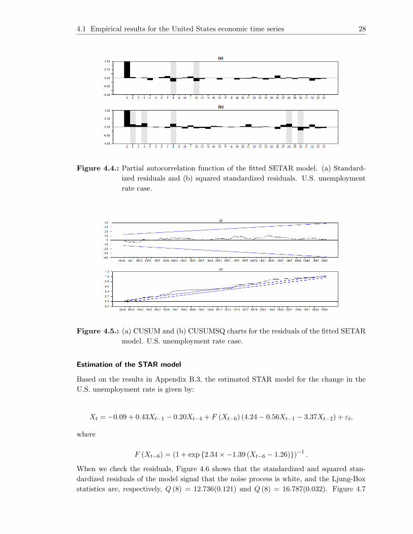
4.1 Empirical results for the United States economic time series 28
Figure 4.4.: Partial autocorrelation function of the fitted SETAR model. (a) Standard-
ized residuals and (b) squared standardized residuals. U.S. unemployment
rate case.
Figure 4.5.: (a) CUSUM and (b) CUSUMSQ charts for the residuals of the fitted SETAR
model. U.S. unemployment rate case.
Estimation of the STAR model
Based on the results in Appendix B.3, the estimated STAR model for the change in the
U.S. unemployment rate is given by:
Xt = −0.09 + 0.43Xt−1 − 0.20Xt−4 + F (Xt−6) (4.24− 0.56Xt−1 − 3.37Xt−2) + εt,
where
F (Xt−6) = (1 + exp {2.34×−1.39 (Xt−6 − 1.26)})−1 .
When we check the residuals, Figure 4.6 shows that the standardized and squared stan-
dardized residuals of the model signal that the noise process is white, and the Ljung-Box
statistics are, respectively, Q (8) = 12.736(0.121) and Q (8) = 16.787(0.032). Figure 4.7
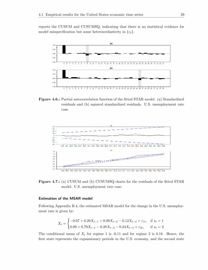
4.1 Empirical results for the United States economic time series 29
reports the CUSUM and CUSUMSQ, indicating that there is no statistical evidence for
model misspecification but some heteroscedasticity in {εt}.
Figure 4.6.: Partial autocorrelation function of the fitted STAR model. (a) Standardized
residuals and (b) squared standardized residuals. U.S. unemployment rate
case.
Figure 4.7.: (a) CUSUM and (b) CUSUMSQ charts for the residuals of the fitted STAR
model. U.S. unemployment rate case.
Estimation of the MSAR model
Following Appendix B.4, the estimated MSAR model for the change in the U.S. unemploy-
ment rate is given by:
Xt =
{−0.07 + 0.28Xt−1 + 0.09Xt−2 − 0.12Xt−4 + ε1t, if st = 1
0.09 + 0.79Xt−1 − 0.28Xt−2 − 0.24Xt−4 + ε2t, if st = 2.
The conditional mean of Xt for regime 1 is -0.11 and for regime 2 is 0.18. Hence, the
first state represents the expansionary periods in the U.S. economy, and the second state

4.1 Empirical results for the United States economic time series 30
represents the contractions. The sample variances of ε1t and ε2t are 0.03 and 0.17, respec-
tively24.
When we check this model, Figure 4.8 shows that the standardized and squared standard-
ized residuals of the model slightly signal that some nonlinear structure in the data is not ex-
plained by the model, and the Ljung-Box statistics are, respectively, Q (8) = 57.784(0.000)
and Q (8) = 2.919(0.939). Figure 4.9 reports the CUSUM and CUSUMSQ, which indicate
that there is statistical evidence for model misspecification and heteroscedasticity in {εt}.
Figure 4.8.: Partial autocorrelation function of the fitted MSAR model. (a) Standardized
residuals and (b) squared standardized residuals. U.S. unemployment rate
case.
Figure 4.9.: (a) CUSUM and (b) CUSUMSQ charts for the residuals of the fitted MSAR
model. U.S. unemployment rate case.
24 The state transition probability p(i, j) gives the probability of moving to state i from j. Thus,
the probabilities of moving from one state to the other are p (st = 2|st−1 = 1) = 0.07(0.03) and
p (st = 1|st−1 = 2) = 0.09(0.05), where the number in parenthesis is the standard error. Addition-
ally, the unconditional probability that the process is in regime 1 is 0.56 and that it is in regime 2 is
0.44. The coefficients also allow us to identify that the probability that an expansion is followed by
another expansion period is p (1, 1) = 0.93, and that the probability that a contraction is followed by
another contraction period is p (2, 2) = 0.91.

4.1 Empirical results for the United States economic time series 31
Estimation of the AR model
We estimate an AR(3) model for the change in the US unemployment rate25, which is
given by:
(1− 0.730B + 0.118B2 + 0.144B3
)Xt = at, σ2a = 0.10.
The standard errors of the coefficients are 0.07, 0.09, and 0.07, respectively. When we check
the residuals, Figure 4.10 shows that the standardized and the squared standardized resid-
uals slightly signal that some linear structure in the data is not explained by the model, and
the Ljung-Box statistics are, respectively, Q (8) = 19.011(0.015) and Q (8) = 23.570(0.003).
Figure 4.11 shows the CUSUM that indicates there is no statistical evidence for model mis-
specification, and the CUSUMSQ that shows statistical evidence for heteroscedasticity in
{εt}.
Figure 4.10.: Partial autocorrelation function of the fitted AR model. (a) Standardized
residuals and (b) squared standardized residuals. U.S. unemployment rate
case.
Figure 4.11.: (a) CUSUM and (b) CUSUMSQ charts for the residuals of the fitted AR
model. U.S. unemployment rate case.
25 As reported by the Augmented Dickey-Fuller (ADF) (p−value = 0.000), Phillips Perron (PP) (p−value =
0.000) and Kwiatkowski-Phillips-Schmidt-Shin (KPSS) (Test statistic = 0.055 and Critical value =
0.463, the change in the unemployment rate is stationary at the 5% significance level.
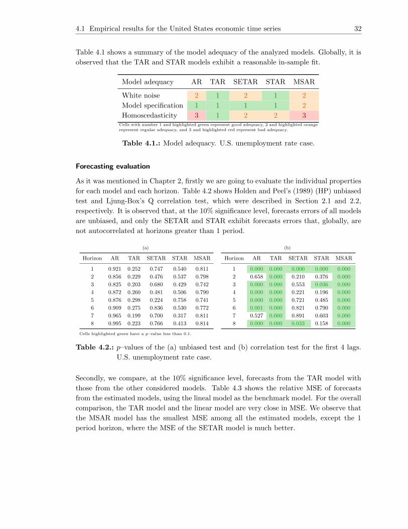
4.1 Empirical results for the United States economic time series 32
Table 4.1 shows a summary of the model adequacy of the analyzed models. Globally, it is
observed that the TAR and STAR models exhibit a reasonable in-sample fit.
Model adequacy AR TAR SETAR STAR MSAR
White noise 2 1 2 1 2
Model specification 1 1 1 1 2
Homoscedasticity 3 1 2 2 3Cells with number 1 and highlighted green represent good adequacy, 2 and highlighted orange
represent regular adequacy, and 3 and highlighted red represent bad adequacy.
Table 4.1.: Model adequacy. U.S. unemployment rate case.
Forecasting evaluation
As it was mentioned in Chapter 2, firstly we are going to evaluate the individual properties
for each model and each horizon. Table 4.2 shows Holden and Peel’s (1989) (HP) unbiased
test and Ljung-Box’s Q correlation test, which were described in Section 2.1 and 2.2,
respectively. It is observed that, at the 10% significance level, forecasts errors of all models
are unbiased, and only the SETAR and STAR exhibit forecasts errors that, globally, are
not autocorrelated at horizons greater than 1 period.
(a)
Horizon AR TAR SETAR STAR MSAR
1 0.921 0.252 0.747 0.540 0.811
2 0.856 0.229 0.476 0.537 0.798
3 0.825 0.203 0.680 0.429 0.742
4 0.872 0.260 0.481 0.506 0.790
5 0.876 0.298 0.224 0.758 0.741
6 0.909 0.275 0.836 0.530 0.772
7 0.965 0.199 0.700 0.317 0.811
8 0.995 0.223 0.766 0.413 0.814
(b)
Horizon AR TAR SETAR STAR MSAR
1 0.000 0.000 0.000 0.000 0.000
2 0.658 0.000 0.210 0.376 0.000
3 0.000 0.000 0.553 0.036 0.000
4 0.000 0.000 0.221 0.196 0.000
5 0.000 0.000 0.721 0.485 0.000
6 0.001 0.000 0.821 0.790 0.000
7 0.527 0.000 0.891 0.603 0.000
8 0.000 0.000 0.033 0.158 0.000
Cells highlighted green have a p–value less than 0.1.
Table 4.2.: p–values of the (a) unbiased test and (b) correlation test for the first 4 lags.
U.S. unemployment rate case.
Secondly, we compare, at the 10% significance level, forecasts from the TAR model with
those from the other considered models. Table 4.3 shows the relative MSE of forecasts
from the estimated models, using the lineal model as the benchmark model. For the overall
comparison, the TAR model and the linear model are very close in MSE. We observe that
the MSAR model has the smallest MSE among all the estimated models, except the 1
period horizon, where the MSE of the SETAR model is much better.
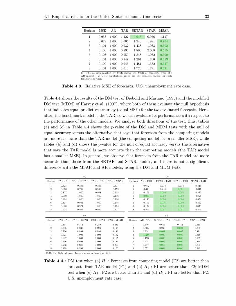
4.1 Empirical results for the United States economic time series 33
Horizon MSE AR TAR SETAR STAR MSAR
1 0.053 1.000 1.127 0.943 0.956 1.117
2 0.079 1.000 1.065 1.243 1.981 0.764
3 0.101 1.000 0.937 1.438 1.933 0.602
4 0.106 1.000 0.893 1.800 2.068 0.575
5 0.103 1.000 0.950 1.848 1.932 0.600
6 0.101 1.000 0.947 1.261 1.700 0.613
7 0.100 1.000 0.946 1.481 1.582 0.627
8 0.101 1.000 1.010 1.723 1.771 0.631
(1) The column marked by MSE shows the MSE of forecasts from the
AR model. (2) Cells highlighted green are the smallest values for each
forecasts horizon.
Table 4.3.: Relative MSE of forecasts. U.S. unemployment rate case.
Table 4.4 shows the results of the DM test of Diebold and Mariano (1995) and the modified
DM test (MDM) of Harvey et al. (1997), where both of them evaluate the null hypothesis
that indicates equal predictive accuracy (equal MSE) for the two evaluated forecasts. Here-
after, the benchmark model is the TAR, so we can evaluate its performance with respect to
the performance of the other models. We analyze both directions of the test, thus, tables
(a) and (c) in Table 4.4 shows the p-value of the DM and MDM tests with the null of
equal accuracy versus the alternative that says that forecasts from the competing models
are more accurate than the TAR model (the competing model has a smaller MSE); while
tables (b) and (d) shows the p-value for the null of equal accuracy versus the alternative
that says the TAR model is more accurate than the competing models (the TAR model
has a smaller MSE). In general, we observe that forecasts from the TAR model are more
accurate than those from the SETAR and STAR models, and there is not a significant
difference with the MSAR and AR models, using the DM and MDM tests.
(a)
Horizon TAR - AR TAR - SETAR TAR - STAR TAR - MSAR
1 0.328 0.286 0.266 0.477
2 0.310 0.752 0.999 0.159
3 0.827 1.000 0.998 0.148
4 0.990 1.000 1.000 0.146
5 0.864 1.000 1.000 0.126
6 0.827 0.984 1.000 0.148
7 0.828 0.974 1.000 0.164
8 0.424 0.993 0.999 0.127
(b)
Horizon AR - TAR SETAR - TAR STAR - TAR MSAR - TAR
1 0.672 0.714 0.734 0.523
2 0.690 0.248 0.001 0.841
3 0.173 0.000 0.002 0.852
4 0.010 0.000 0.000 0.854
5 0.136 0.000 0.000 0.874
6 0.173 0.016 0.000 0.852
7 0.172 0.026 0.000 0.836
8 0.576 0.007 0.001 0.873
(c)
Horizon TAR - AR TAR - SETAR TAR - STAR TAR - MSAR
1 0.354 0.314 0.289 0.481
2 0.335 0.731 0.996 0.193
3 0.766 0.999 0.993 0.186
4 0.971 1.000 1.000 0.182
5 0.807 1.000 1.000 0.165
6 0.776 0.998 1.000 0.184
7 0.783 0.981 1.000 0.200
8 0.428 0.998 1.000 0.160
(d)
Horizon AR - TAR SETAR - TAR STAR - TAR MSAR - TAR
1 0.646 0.686 0.711 0.519
2 0.665 0.269 0.004 0.807
3 0.234 0.001 0.007 0.814
4 0.029 0.000 0.000 0.818
5 0.193 0.000 0.000 0.835
6 0.224 0.002 0.000 0.816
7 0.217 0.019 0.000 0.800
8 0.572 0.002 0.000 0.840
Cells highlighted green have a p–value less than 0.1.
Table 4.4.: DM test when (a) H1 : Forecasts from competing model (F2) are better than
forecasts from TAR model (F1) and (b) H1 : F1 are better than F2; MDM
test when (c) H1 : F2 are better than F1 and (d) H1 : F1 are better than F2.
U.S. unemployment rate case.
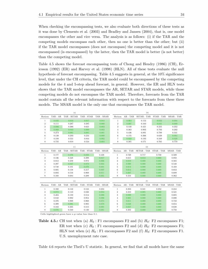
4.1 Empirical results for the United States economic time series 34
When checking the encompassing tests, we also evaluate both directions of these tests as
it was done by Clements et al. (2003) and Bradley and Jansen (2004), that is, one model
encompasses the other and vice versa. The analysis is as follows: (i) if the TAR and the
competing models encompass each other, then no one is better than the other; but (ii)
if the TAR model encompasses (does not encompass) the competing model and it is not
encompassed (is encompassed) by the latter, then the TAR model is better (is not better)
than the competing model.
Table 4.5 shows the forecast encompassing tests of Chong and Hendry (1986) (CH), Er-
icsson (1992) (ER) and Harvey et al. (1998) (HLN). All of these tests evaluate the null
hypothesis of forecast encompassing. Table 4.5 suggests in general, at the 10% significance
level, that under the CH criteria, the TAR model could be encompassed by the competing
models for the 4 and 5-step ahead forecast, in general. However, the ER and HLN tests
shows that the TAR model encompasses the AR, SETAR and STAR models, while those
competing models do not encompass the TAR model. Therefore, forecasts from the TAR
model contain all the relevant information with respect to the forecasts from these three
models. The MSAR model is the only one that encompasses the TAR model.
(a)
Horizon TAR - AR TAR - SETAR TAR - STAR TAR - MSAR
1 0.035 0.016 0.017 0.044
2 0.111 0.267 0.385 0.000
3 0.086 0.366 0.621 0.003
4 0.068 0.043 0.069 0.002
5 0.273 0.081 0.081 0.001
6 0.138 0.203 0.234 0.000
7 0.188 0.531 0.844 0.002
8 0.735 0.918 0.524 0.004
(b)
Horizon AR - TAR SETAR - TAR STAR - TAR MSAR - TAR
1 0.064 0.153 0.033 0.004
2 0.007 0.163 0.041 0.000
3 0.440 0.421 0.255 0.352
4 0.363 0.903 0.793 0.202
5 0.436 0.891 0.789 0.341
6 0.155 0.366 0.639 0.064
7 0.023 0.193 0.349 0.029
8 0.385 0.571 0.765 0.770
(c)
Horizon TAR - AR TAR - SETAR TAR - STAR TAR - MSAR
1 0.177 0.076 0.058 0.438
2 0.136 0.248 0.299 0.017
3 0.812 0.259 0.972 0.006
4 0.297 0.047 0.073 0.004
5 0.748 0.101 0.078 0.001
6 0.805 0.158 0.217 0.007
7 0.693 0.516 0.969 0.011
8 0.168 0.684 0.289 0.001
(d)
Horizon AR - TAR SETAR - TAR STAR - TAR MSAR - TAR
1 0.729 0.717 0.730 0.509
2 0.615 0.013 0.000 0.958
3 0.019 0.000 0.000 0.565
4 0.000 0.000 0.000 0.548
5 0.013 0.000 0.000 0.458
6 0.012 0.000 0.000 0.653
7 0.007 0.000 0.000 0.689
8 0.316 0.000 0.000 0.362
(e)
Horizon TAR - AR TAR - SETAR TAR - STAR TAR - MSAR
1 0.160 0.142 0.124 0.234
2 0.072 0.143 0.826 0.053
3 0.404 0.150 0.514 0.086
4 0.842 0.982 0.954 0.086
5 0.376 0.969 0.968 0.074
6 0.399 0.091 0.905 0.078
7 0.343 0.265 0.515 0.091
8 0.076 0.340 0.130 0.081
(f)
Horizon AR - TAR SETAR - TAR STAR - TAR MSAR - TAR
1 0.353 0.341 0.352 0.244
2 0.310 0.005 0.000 0.521
3 0.039 0.000 0.000 0.685
4 0.001 0.000 0.000 0.690
5 0.011 0.000 0.000 0.722
6 0.048 0.000 0.000 0.654
7 0.057 0.000 0.000 0.638
8 0.202 0.000 0.000 0.750
Cells highlighted green have a p–value less than 0.1.
Table 4.5.: CH test when (a) H0 : F1 encompasses F2 and (b) H0: F2 encompasses F1;
ER test when (c) H0 : F1 encompasses F2 and (d) H0: F2 encompasses F1;
HLN test when (e) H0 : F1 encompasses F2 and (f) H0: F2 encompasses F1.
U.S. unemployment rate case.
Table 4.6 reports the Theil’s U statistic. In general, we find that all models have the same
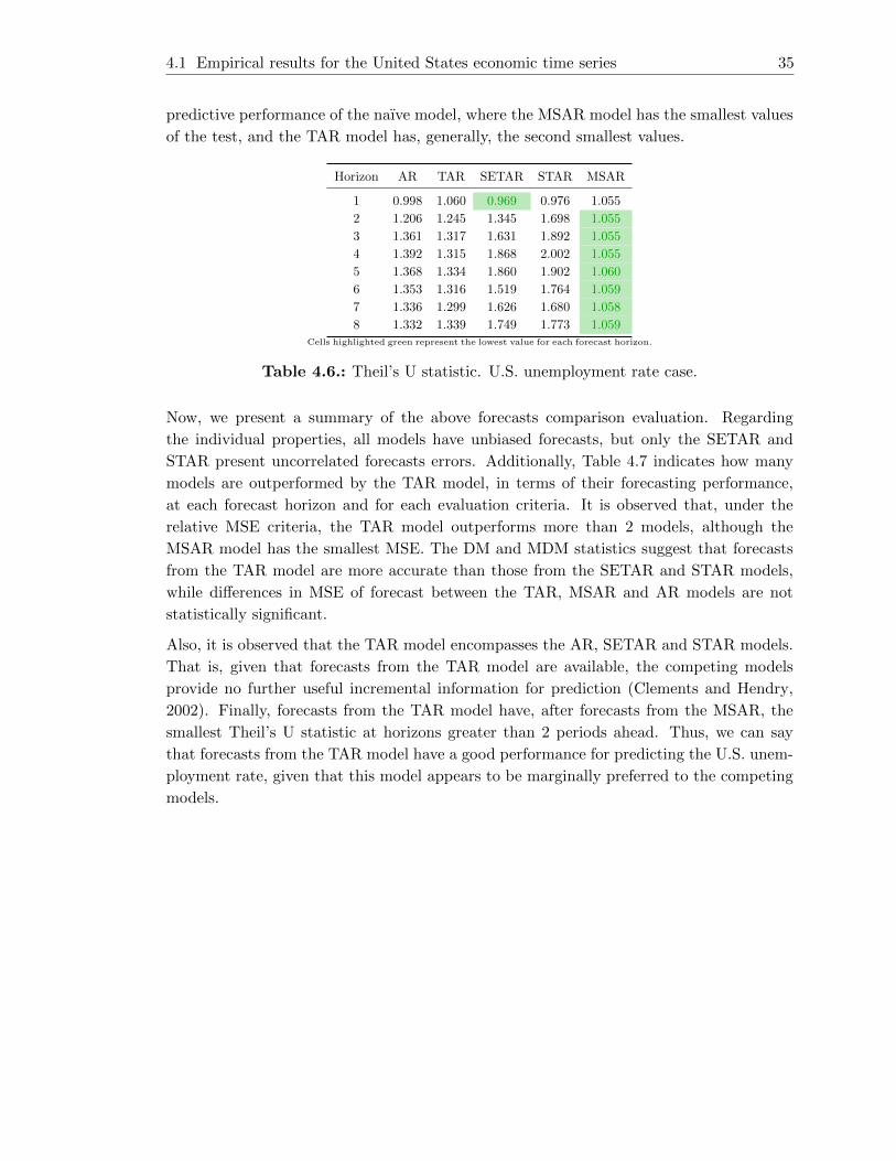
4.1 Empirical results for the United States economic time series 35
predictive performance of the naıve model, where the MSAR model has the smallest values
of the test, and the TAR model has, generally, the second smallest values.
Horizon AR TAR SETAR STAR MSAR
1 0.998 1.060 0.969 0.976 1.055
2 1.206 1.245 1.345 1.698 1.055
3 1.361 1.317 1.631 1.892 1.055
4 1.392 1.315 1.868 2.002 1.055
5 1.368 1.334 1.860 1.902 1.060
6 1.353 1.316 1.519 1.764 1.059
7 1.336 1.299 1.626 1.680 1.058
8 1.332 1.339 1.749 1.773 1.059Cells highlighted green represent the lowest value for each forecast horizon.
Table 4.6.: Theil’s U statistic. U.S. unemployment rate case.
Now, we present a summary of the above forecasts comparison evaluation. Regarding
the individual properties, all models have unbiased forecasts, but only the SETAR and
STAR present uncorrelated forecasts errors. Additionally, Table 4.7 indicates how many
models are outperformed by the TAR model, in terms of their forecasting performance,
at each forecast horizon and for each evaluation criteria. It is observed that, under the
relative MSE criteria, the TAR model outperforms more than 2 models, although the
MSAR model has the smallest MSE. The DM and MDM statistics suggest that forecasts
from the TAR model are more accurate than those from the SETAR and STAR models,
while differences in MSE of forecast between the TAR, MSAR and AR models are not
statistically significant.
Also, it is observed that the TAR model encompasses the AR, SETAR and STAR models.
That is, given that forecasts from the TAR model are available, the competing models
provide no further useful incremental information for prediction (Clements and Hendry,
2002). Finally, forecasts from the TAR model have, after forecasts from the MSAR, the
smallest Theil’s U statistic at horizons greater than 2 periods ahead. Thus, we can say
that forecasts from the TAR model have a good performance for predicting the U.S. unem-
ployment rate, given that this model appears to be marginally preferred to the competing
models.

4.1 Empirical results for the United States economic time series 36
Horizon Relative MSE DM - MDM Encompassing tests U-Theil
1 0 0 0 0
2 2 1 2 2
(SETAR, STAR) (STAR) (STAR, AR) (SETAR, STAR)
3 3 2 3 2
(SETAR, STAR, AR) (SETAR, STAR) (SETAR, STAR, AR) (SETAR, STAR)
4 3 3 3 3
(SETAR, STAR, AR) (SETAR, STAR, AR) (SETAR, STAR, AR) (SETAR, STAR, AR)
5 3 2 3 3
(SETAR, STAR, AR) (SETAR, STAR) (SETAR, STAR, AR) (SETAR, STAR, AR)
6 3 2 3 3
(SETAR, STAR, AR) (SETAR, STAR) (SETAR, STAR, AR) (SETAR, STAR, AR)
7 3 2 3 3
(SETAR, STAR, AR) (SETAR, STAR) (SETAR, STAR, AR) (SETAR, STAR, AR)
8 3 2 2 2
(SETAR, STAR, AR) (SETAR, STAR) (SETAR, STAR) (SETAR, STAR)
(1) Cells highlighted green report that the TAR model outperforms 3 or 4 models, highlighted orange report
that the TAR model outperforms 1 or 2 models, and highlighted red report that the TAR model does not
outperform any model. (2) Models in parenthesis are outperformed by the TAR model.
Table 4.7.: Summary of the forecasting performance of the TAR model. U.S. unemploy-
ment rate case.
Finally, we compare the TAR model with the SETAR and STAR models based on their
ability to describe the predictive distributions of the time series26, in terms of the capacity
to handle cycles. As it was mentioned in Chapter 2, we make this comparison exercise
based on Wong and Li (2000), who suggest that the predictive distribution is unimodal
when the series is ascending to a peak and bimodal when the series is descending to a
trough.
Figure 4.12 shows the predictive distributions for horizons from 1 to 8, when the forecast
origin is 2008:03. Based on the business cycle contractions from peak to trough of the
NBER, there is a business contraction from 2007:04 to 2009:02. According to this, the
predictive distributions of the TAR model tend to be bimodal when the time series is in a
trough between 2008:04 and 2009:02 (positive increments of the unemployment rate) and
become more unimodal when the time series is regaining an expansionist trend (negative
increments of the unemployment rate). The predictive distributions of the SETAR and
STAR models do not tend to be bimodal when the time series is in the peak. This suggests
that the predictive distributions of the TAR model seem to handle cycles of the times series
reasonably well.
26 Hereafter, for all models and all the economic time series, we generate the 1 to 8-step predictive distri-
butions for the U.S. and Colombian cases, using the Monte Carlo approach with 2000 replications.
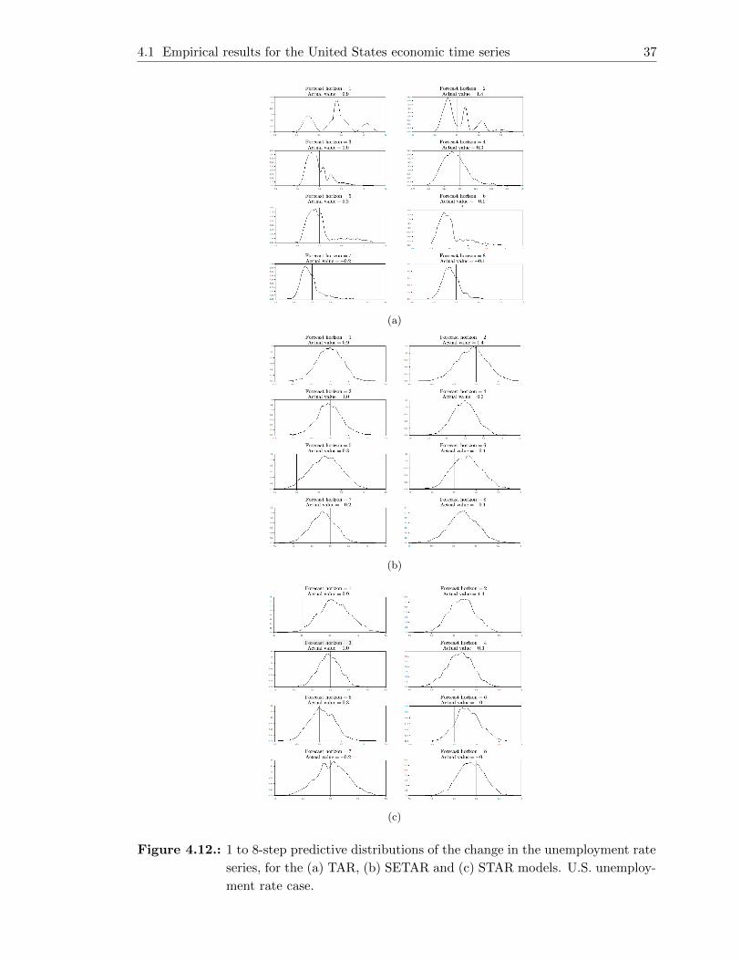
4.1 Empirical results for the United States economic time series 37
(a)
(b)
(c)
Figure 4.12.: 1 to 8-step predictive distributions of the change in the unemployment rate
series, for the (a) TAR, (b) SETAR and (c) STAR models. U.S. unemploy-
ment rate case.

4.1 Empirical results for the United States economic time series 38
4.1.2. Gross domestic product
Description of the data
We use the annual growth rate of the seasonally adjusted U.S. quarterly real output, in
billions of chained 2009 Dollars, from 1955:03 to 2016:03 (245 observations), measured by
the U.S. Bureau of Economic Analysis. As the threshold value, we use the term spread
defined in Section 3.2 over the same period, that is, the difference between the 10-Year
Treasury Constant Maturity rate as the long-term government bond rate, and the effective
federal funds rate as the overnight rate.
For the forecast comparison, we denote Xt = [log(GDP t)− log(GDP t−4)] ∗ 100 as the
annual growth rate of the real GDP, and Zt = (govt − overnightt) the spread term, where
govt is the 10-Year Treasury Constant Maturity rate, and overnightt is the effective federal
funds at time t. Both series are plotted in Figure 4.13 that shows a similar behavior of
these series during contractions periods. The shading areas denote the business cycle
contractions from peak to trough.
Figure 4.13.: (a) Time plot of the annual growth rate of U.S. real GDP and (b) time plot
of U.S. term spread.
We use as the training subsample, data from 1955:03 to 1998:02 (172 observations). The re-
maining observations are reserved for the out-of-sample forecasting evaluation. A sequence
of 1 to 8-step ahead forecasts are generated until we compute 73 1-step ahead forecasts,
down to 66 8-step ahead forecast.
Estimation of models
Based on results in Appendix C, Table 4.8 shows that globally, the TAR model presents
the best reasonable in-sample fit.

4.1 Empirical results for the United States economic time series 39
Model adequacy AR TAR SETAR STAR MSAR
White noise 3 1 2 3 2
Model specification 1 1 1 1 3
Homoscedasticity 3 2 3 3 3Cells with number 1 and highlighted green represent good adequacy, 2 and highlighted orange
represent regular adequacy, and 3 and highlighted red represent bad adequacy.
Table 4.8.: Model adequacy. U.S. GDP case.
Forecasting evaluation
Table 4.9 shows that at the 10% significance level, only forecasts errors of the TAR model
are unbiased, and only the SETAR and STAR exhibit forecasts errors that, globally, are
not autocorrelated at horizons greater than 4 periods.
(a)
Horizon AR TAR SETAR STAR MSAR
1 0.001 0.601 0.016 0.019 0.016
2 0.000 0.689 0.072 0.001 0.013
3 0.000 0.432 0.107 0.004 0.006
4 0.000 0.373 0.091 0.016 0.006
5 0.000 0.302 0.042 0.000 0.006
6 0.000 0.202 0.034 0.000 0.004
7 0.000 0.180 0.015 0.000 0.003
8 0.000 0.163 0.000 0.000 0.003
(b)
Horizon AR TAR SETAR STAR MSAR
1 0.000 0.000 0.000 0.000 0.000
2 0.000 0.000 0.000 0.406 0.000
3 0.000 0.000 0.036 0.193 0.000
4 0.000 0.000 0.099 0.021 0.000
5 0.000 0.000 0.272 0.189 0.000
6 0.000 0.000 0.509 0.304 0.000
7 0.000 0.000 0.314 0.727 0.000
8 0.000 0.000 0.581 0.776 0.000
Cells highlighted green have a p–value less than 0.1.
Table 4.9.: p–values of the (a) unbiased test and (b) correlation test for the first 4 lags.
U.S. GDP case.
Now, we present the forecast comparison at the 10% significance level. Table 4.10 shows,
for the overall comparison, that the TAR model and the linear model are very close in
MSE of forecasts, but the MSAR model has the smallest MSE among all the estimated
models, except for the 1-step ahead forecast, where the MSE of the TAR model is much
better.
Horizon MSE AR TAR SETAR STAR MSAR
1 0.546 1.000 0.957 1.654 1.124 0.995
2 1.579 1.000 0.976 2.034 2.700 0.348
3 2.917 1.000 1.051 1.845 2.305 0.184
4 4.399 1.000 1.079 1.928 1.971 0.124
5 5.059 1.000 1.081 1.841 1.478 0.109
6 5.265 1.000 1.048 1.630 1.442 0.106
7 5.233 1.000 1.063 1.511 1.730 0.107
8 5.062 1.000 1.105 1.913 1.798 0.112
(1) The column marked by MSE shows the MSE of forecasts from the
AR model. (2) Cells highlighted green are the smallest values for each
forecasts horizon.
Table 4.10.: Relative MSE of forecasts. U.S. GDP case.

4.1 Empirical results for the United States economic time series 40
Henceforth, we define the TAR model as the benchmark model. Table 4.11, that shows
the results of the DM and MDM tests, suggests that forecasts from the TAR model are
more accurate than those from the SETAR and STAR models, and there is no significant
difference with those from the AR model. However, forecasts from the MSAR model are
more accurate than those from the TAR model.
(a)
Horizon TAR - AR TAR - SETAR TAR - STAR TAR - MSAR
1 0.642 0.943 0.792 0.629
2 0.580 0.987 1.000 0.004
3 0.356 0.985 0.990 0.003
4 0.293 0.994 0.955 0.003
5 0.307 0.991 0.958 0.002
6 0.383 0.979 0.980 0.003
7 0.347 0.984 0.998 0.002
8 0.241 0.998 0.999 0.003
(b)
Horizon AR - TAR SETAR - TAR STAR - TAR MSAR - TAR
1 0.358 0.057 0.208 0.371
2 0.420 0.013 0.000 0.996
3 0.644 0.015 0.011 0.997
4 0.707 0.006 0.045 0.997
5 0.693 0.009 0.042 0.998
6 0.617 0.021 0.020 0.998
7 0.653 0.016 0.002 0.998
8 0.759 0.002 0.001 0.997
(c)
Horizon TAR - AR TAR - SETAR TAR - STAR TAR - MSAR
1 0.643 0.900 0.743 0.630
2 0.579 0.967 0.997 0.014
3 0.354 0.965 0.993 0.010
4 0.301 0.987 0.961 0.009
5 0.337 0.986 0.955 0.007
6 0.402 0.999 0.965 0.008
7 0.373 1.000 0.994 0.007
8 0.282 1.000 0.996 0.009
(d)
Horizon AR - TAR SETAR - TAR STAR - TAR MSAR - TAR
1 0.357 0.100 0.257 0.370
2 0.421 0.033 0.003 0.986
3 0.646 0.035 0.007 0.990
4 0.699 0.013 0.039 0.991
5 0.663 0.014 0.045 0.993
6 0.598 0.001 0.035 0.992
7 0.627 0.000 0.006 0.993
8 0.718 0.000 0.004 0.991
Cells highlighted green have a p–value less than 0.1.
Table 4.11.: DM test when (a) H1 : Forecasts from competing model (F2) are better than
forecasts from TAR model (F1) and (b) H1 : F1 are better than F2; MDM
test when (c) H1 : F2 are better than F1 and (d) H1 : F1 are better than
F2. U.S. GDP case.
Table 4.12 shows, under the CH test, that the TAR model could encompass the linear
model. However, under the ER and HLN tests, the TAR, SETAR, STAR and AR models
do not encompass each other, so forecasts from all models contain all the same useful
information for prediction. Only the MSAR model do encompasses the TAR model.

4.1 Empirical results for the United States economic time series 41
(a)
Horizon TAR - AR TAR - SETAR TAR - STAR TAR - MSAR
1 0.940 0.783 0.737 0.974
2 0.988 0.676 0.766 0.123
3 0.732 0.814 0.847 0.097
4 0.622 0.903 0.708 0.067
5 0.517 0.965 0.724 0.057
6 0.422 0.819 0.603 0.058
7 0.385 0.745 0.503 0.079
8 0.357 0.412 0.445 0.075
(b)
Horizon AR - TAR SETAR - TAR STAR - TAR MSAR - TAR
1 0.129 0.911 0.895 0.370
2 0.074 0.714 0.500 0.270
3 0.020 0.638 0.159 0.053
4 0.012 0.562 0.165 0.025
5 0.005 0.332 0.014 0.013
6 0.003 0.384 0.015 0.060
7 0.001 0.134 0.002 0.004
8 0.001 0.018 0.000 0.005
(c)
Horizon TAR - AR TAR - SETAR TAR - STAR TAR - MSAR
1 0.002 0.003 0.000 0.005
2 0.000 0.019 0.033 0.000
3 0.000 0.001 0.001 0.000
4 0.000 0.000 0.000 0.000
5 0.000 0.000 0.000 0.000
6 0.000 0.000 0.000 0.000
7 0.000 0.000 0.009 0.000
8 0.000 0.007 0.012 0.000
(d)
Horizon AR - TAR SETAR - TAR STAR - TAR MSAR - TAR
1 0.000 0.000 0.000 0.001
2 0.000 0.000 0.000 0.446
3 0.000 0.000 0.000 0.727
4 0.000 0.000 0.000 0.358
5 0.000 0.000 0.000 0.337
6 0.000 0.000 0.000 0.826
7 0.001 0.000 0.000 0.357
8 0.001 0.000 0.000 0.431
(e)
Horizon TAR - AR TAR - SETAR TAR - STAR TAR - MSAR
1 0.001 0.039 0.010 0.001
2 0.016 0.068 0.090 0.000
3 0.017 0.029 0.043 0.000
4 0.017 0.022 0.020 0.002
5 0.017 0.012 0.014 0.001
6 0.018 0.001 0.022 0.001
7 0.012 0.001 0.033 0.001
8 0.009 0.020 0.041 0.001
(f)
Horizon AR - TAR SETAR - TAR STAR - TAR MSAR - TAR
1 0.003 0.036 0.064 0.005
2 0.000 0.005 0.001 0.213
3 0.000 0.003 0.009 0.631
4 0.000 0.005 0.019 0.792
5 0.001 0.002 0.002 0.797
6 0.001 0.000 0.002 0.584
7 0.001 0.000 0.000 0.787
8 0.001 0.000 0.000 0.757
Cells highlighted green have a p–value less than 0.1.
Table 4.12.: CH test when (a) H0 : F1 encompasses F2 and (b) H0: F2 encompasses F1;
ER test when (c) H0 : F1 encompasses F2 and (d) H0: F2 encompasses F1;
HLN test when (e) H0 : F1 encompasses F2 and (f) H0: F2 encompasses F1.
U.S. GDP case.
Table 4.13 shows that the MSAR model is the only one, among all the evaluated models,
that has a better predictive performance than the naıve model, and the TAR model has
the third-best values of the Theil’s U statistic.
Horizon AR TAR SETAR STAR MSAR
1 0.905 0.885 1.164 0.959 0.903
2 1.528 1.510 2.180 2.511 0.901
3 2.079 2.131 2.823 3.156 0.892
4 2.535 2.634 3.521 3.560 0.892
5 2.535 2.808 3.664 3.282 0.892
6 2.735 2.800 3.491 3.284 0.890
7 2.706 2.791 3.327 3.560 0.887
8 2.649 2.785 3.664 3.552 0.888Cells highlighted green represent the lowest value for each forecast horizon.
Table 4.13.: Theil’s U statistic. U.S. GDP case.
As a summary of the above forecasts comparison evaluation, it is observed that only the
TAR model has unbiased forecasts, but the SETAR and STAR present uncorrelated fore-
casts errors for some forecast periods. Additionally, Table 4.14 let us observe a satisfactory
performance of the TAR model. According to the Relative MSE of forecast and the DM

4.1 Empirical results for the United States economic time series 42
and MDM tests, the TAR model has better MSE of forecasts than the SETAR and STAR
models. Regarding the encompassing tests, only the MSAR model encompasses the TAR
model, while the other models contain all the same useful information for prediction than
the TAR model. Additionally, forecasts from the MSAR model are more accurate than
those from the naıve model.
Therefore, from this out-of-sample forecasts comparison, we can conclude that the TAR
model could forecasts the growth rate of the real GDP with a good performance, given that
of the alternatives, the TAR model appears to be marginally preferred to the competing
modes, except the MSAR model that seems to be more competitive according with these
tests.
Horizon Relative MSE DM - MDM Encompassing tests U-Theil
1 4 1 2 4
(AR, SETAR, STAR, MSAR) (SETAR) (AR, STAR) (AR, SETAR, STAR, MSAR)
2 3 2 0 3
(AR, SETAR, STAR) (SETAR, STAR) (AR, SETAR, STAR)
3 2 2 0 2
(SETAR, STAR) (SETAR, STAR) (SETAR, STAR)
4 2 2 0 2
(SETAR, STAR) (SETAR, STAR) (SETAR, STAR)
5 2 2 0 2
(SETAR, STAR) (SETAR, STAR) (SETAR, STAR)
6 2 2 0 2
(SETAR, STAR) (SETAR, STAR) (SETAR, STAR)
7 2 2 0 2
(SETAR, STAR) (SETAR, STAR) (SETAR, STAR)
8 2 2 0 2
(SETAR, STAR) (SETAR, STAR) (SETAR, STAR)
(1) Cells highlighted green report that the TAR model outperforms 3 or 4 models, highlighted orange report
that the TAR model outperforms 1 or 2 models, and highlighted red report that the TAR model does not
outperform any model. (2) Models in parenthesis are outperformed by the TAR model.
Table 4.14.: Summary of the forecasting performance of the TAR model. U.S. GDP case.
Finally, we compare the TAR model with the SETAR and STAR models based on their
ability to describe the predictive distribution of the growth rate of the real GDP, in terms of
the capacity to handle cycles. Figure 4.14 shows the predictive distributions for horizons 1
to 8, when the forecast origin is 2008:04. Based on the business contraction from 2007:04 to
2009:02, which is determined by the NBER, the predictive distributions of the TAR model
tend to be bimodal when the time series is in a through (negative growths of the real
GDP), and become more unimodal when the time series is regaining an expansionist trend
(positive growths of the real GDP). The predictive distributions of the SETAR and STAR
models slightly capture this behavior. This pattern of the predictive distributions is also
observed in other parts of the time series. This suggests that the predictive distributions
of the TAR model seem to handle cycles of the times series reasonably well.
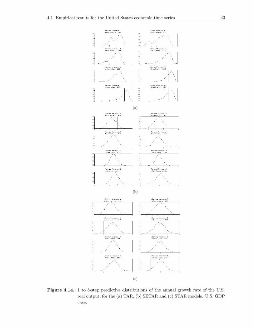
4.1 Empirical results for the United States economic time series 43
(a)
(b)
(c)
Figure 4.14.: 1 to 8-step predictive distributions of the annual growth rate of the U.S.
real output, for the (a) TAR, (b) SETAR and (c) STAR models. U.S. GDP
case.

4.1 Empirical results for the United States economic time series 44
4.1.3. Industrial production index
Description of the data
We analyze the annual growth rate of the seasonally adjusted U.S. quarterly industrial
production index (indpro), from 1960:01 to 2016:03 (227 observations), which was retrieved
from the Federal Reserve Bank of St. Louis (FRED). As the threshold value, we use the
term spread defined in Section 3.2 over the same period.
For the forecast comparison, we denote Xt =[log(Indprot)− log(Indprot−4)
]∗ 100 as the
annual growth rate of the industrial production index (indpro), and Zt, the spread term
defined as the difference between the 10-Year Treasury Constant Maturity rate and the
effective federal funds. Both series are plotted in Figure 4.15 that shows a similar behavior
during contractions periods of these series. The shading areas denote the business cycle
contractions from peak to trough.
Figure 4.15.: (a) Time plot of the annual growth rate of U.S. quarterly industrial pro-
duction index and (b) time plot of U.S. term spread.
We use as the training subsample, the data from 1960:01 to 1999:04 (160 observations).
The remaining observations are reserved for the out-of-sample forecasting evaluation. By
using the procedure mentioned at the beginning of this Chapter, a sequence of 1 to 8-step
ahead forecasts are generated until we compute 67 1-step ahead forecasts down to 60 8-step
ahead forecast.
Estimation of models
Based on the estimation procedure in Appendix D, Table 4.15 shows that, in general, the
TAR shows the best reasonable in-sample fit.
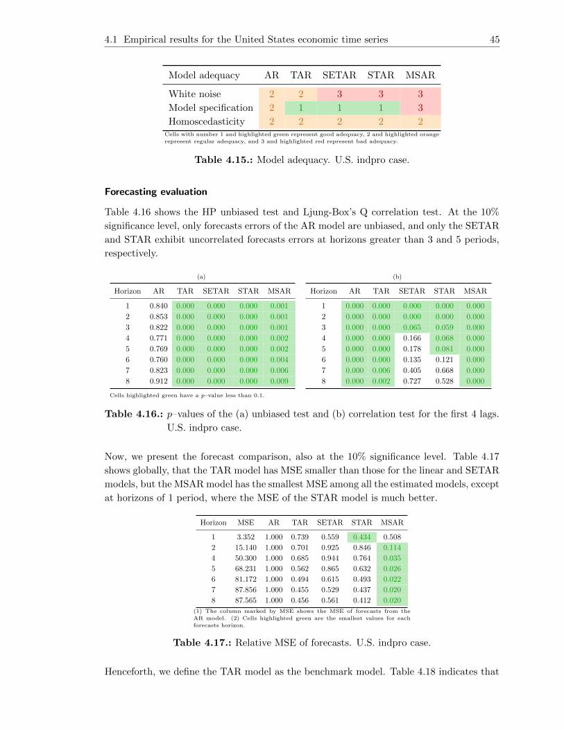
4.1 Empirical results for the United States economic time series 45
Model adequacy AR TAR SETAR STAR MSAR
White noise 2 2 3 3 3
Model specification 2 1 1 1 3
Homoscedasticity 2 2 2 2 2Cells with number 1 and highlighted green represent good adequacy, 2 and highlighted orange
represent regular adequacy, and 3 and highlighted red represent bad adequacy.
Table 4.15.: Model adequacy. U.S. indpro case.
Forecasting evaluation
Table 4.16 shows the HP unbiased test and Ljung-Box’s Q correlation test. At the 10%
significance level, only forecasts errors of the AR model are unbiased, and only the SETAR
and STAR exhibit uncorrelated forecasts errors at horizons greater than 3 and 5 periods,
respectively.
(a)
Horizon AR TAR SETAR STAR MSAR
1 0.840 0.000 0.000 0.000 0.001
2 0.853 0.000 0.000 0.000 0.001
3 0.822 0.000 0.000 0.000 0.001
4 0.771 0.000 0.000 0.000 0.002
5 0.769 0.000 0.000 0.000 0.002
6 0.760 0.000 0.000 0.000 0.004
7 0.823 0.000 0.000 0.000 0.006
8 0.912 0.000 0.000 0.000 0.009
(b)
Horizon AR TAR SETAR STAR MSAR
1 0.000 0.000 0.000 0.000 0.000
2 0.000 0.000 0.000 0.000 0.000
3 0.000 0.000 0.065 0.059 0.000
4 0.000 0.000 0.166 0.068 0.000
5 0.000 0.000 0.178 0.081 0.000
6 0.000 0.000 0.135 0.121 0.000
7 0.000 0.006 0.405 0.668 0.000
8 0.000 0.002 0.727 0.528 0.000
Cells highlighted green have a p–value less than 0.1.
Table 4.16.: p–values of the (a) unbiased test and (b) correlation test for the first 4 lags.
U.S. indpro case.
Now, we present the forecast comparison, also at the 10% significance level. Table 4.17
shows globally, that the TAR model has MSE smaller than those for the linear and SETAR
models, but the MSAR model has the smallest MSE among all the estimated models, except
at horizons of 1 period, where the MSE of the STAR model is much better.
Horizon MSE AR TAR SETAR STAR MSAR
1 3.352 1.000 0.739 0.559 0.434 0.508
2 15.140 1.000 0.701 0.925 0.846 0.114
4 50.300 1.000 0.685 0.944 0.764 0.035
5 68.231 1.000 0.562 0.865 0.632 0.026
6 81.172 1.000 0.494 0.615 0.493 0.022
7 87.856 1.000 0.455 0.529 0.437 0.020
8 87.565 1.000 0.456 0.561 0.412 0.020
(1) The column marked by MSE shows the MSE of forecasts from the
AR model. (2) Cells highlighted green are the smallest values for each
forecasts horizon.
Table 4.17.: Relative MSE of forecasts. U.S. indpro case.
Henceforth, we define the TAR model as the benchmark model. Table 4.18 indicates that

4.1 Empirical results for the United States economic time series 46
forecasts from the TAR model are more accurate than those from the SETAR at horizons
greater than 1, and there is no significant difference with forecasts form the STAR and AR
models. However, forecasts from the MSAR model are more accurate than those from the
TAR model.
(a)
Horizon TAR - AR TAR - SETAR TAR - STAR TAR - MSAR
1 0.755 0.004 0.028 0.006
2 0.765 0.992 0.914 0.017
3 0.781 0.988 0.879 0.016
4 0.777 0.970 0.765 0.016
5 0.862 0.981 0.789 0.015
6 0.893 0.920 0.494 0.014
7 0.906 0.916 0.425 0.015
8 0.898 0.983 0.316 0.022
(b)
Horizon AR - TAR SETAR - TAR STAR - TAR MSAR - TAR
1 0.245 0.996 0.972 0.994
2 0.235 0.008 0.086 0.983
3 0.219 0.012 0.121 0.984
4 0.223 0.030 0.235 0.984
5 0.138 0.019 0.211 0.985
6 0.107 0.080 0.506 0.987
7 0.094 0.084 0.575 0.985
8 0.102 0.017 0.684 0.978
(c)
Horizon TAR - AR TAR - SETAR TAR - STAR TAR - MSAR
1 0.748 0.004 0.032 0.015
2 0.761 1.000 0.893 0.042
3 0.780 0.999 0.863 0.040
4 0.778 0.977 0.745 0.041
5 0.838 0.979 0.772 0.042
6 0.851 0.926 0.495 0.037
7 0.856 0.903 0.436 0.039
8 0.844 0.991 0.338 0.050
(d)
Horizon AR - TAR SETAR - TAR STAR - TAR MSAR - TAR
1 0.252 0.996 0.968 0.985
2 0.239 0.000 0.107 0.958
3 0.220 0.001 0.137 0.960
4 0.222 0.023 0.255 0.959
5 0.162 0.021 0.228 0.958
6 0.149 0.074 0.505 0.963
7 0.144 0.097 0.564 0.961
8 0.156 0.009 0.662 0.950
Cells highlighted green have a p–value less than 0.1.
Table 4.18.: DM test when (a) H1 : Forecasts from competing model (F2) are better than
forecasts from TAR model (F1) and (b) H1 : F1 are better than F2; MDM
test when (c) H1 : F2 are better than F1 and (d) H1 : F1 are better than
F2. U.S. indpro case.
Table 4.19 shows, under the CH test, that the TAR model could encompass the linear
model for the first 4-step ahead forecasts, and the STAR model at horizon greater than
3. However, under the ER and HLN tests and for the overall comparison, the TAR could
encompass the linear model, while the TAR, SETAR and STAR do not encompass each
other, and the MSAR model could encompass the benchmark model.

4.1 Empirical results for the United States economic time series 47
(a)
Horizon TAR - AR TAR - SETAR TAR - STAR TAR - MSAR
1 0.752 0.824 0.411 0.779
2 0.930 0.165 0.907 0.124
3 0.573 0.044 0.594 0.021
4 0.253 0.032 0.503 0.004
5 0.013 0.106 0.367 0.001
6 0.002 0.142 0.222 0.003
7 0.003 0.070 0.128 0.007
8 0.006 0.036 0.090 0.017
(b)
Horizon AR - TAR SETAR - TAR STAR - TAR MSAR - TAR
1 0.015 0.613 0.391 0.622
2 0.005 0.461 0.695 0.061
3 0.028 0.015 0.221 0.001
4 0.049 0.001 0.052 0.002
5 0.060 0.002 0.034 0.029
6 0.070 0.023 0.014 0.024
7 0.105 0.022 0.004 0.034
8 0.146 0.017 0.005 0.041
(c)
Horizon TAR - AR TAR - SETAR TAR - STAR TAR - MSAR
1 0.179 0.000 0.000 0.000
2 0.246 0.016 0.000 0.000
3 0.247 0.012 0.003 0.000
4 0.227 0.029 0.000 0.000
5 0.427 0.174 0.001 0.000
6 0.610 0.025 0.000 0.090
7 0.688 0.013 0.004 0.000
8 0.595 0.038 0.005 0.000
(d)
Horizon AR - TAR SETAR - TAR STAR - TAR MSAR - TAR
1 0.004 0.495 0.493 0.243
2 0.004 0.000 0.000 0.044
3 0.002 0.000 0.000 0.008
4 0.002 0.000 0.000 0.011
5 0.000 0.000 0.000 0.090
6 0.000 0.000 0.000 0.090
7 0.000 0.000 0.013 0.094
8 0.000 0.000 0.062 0.091
(e)
Horizon TAR - AR TAR - SETAR TAR - STAR TAR - MSAR
1 0.064 0.000 0.004 0.000
2 0.086 0.014 0.014 0.008
3 0.077 0.012 0.028 0.012
4 0.074 0.021 0.020 0.015
5 0.162 0.116 0.022 0.013
6 0.270 0.046 0.006 0.012
7 0.321 0.055 0.011 0.013
8 0.258 0.054 0.009 0.020
(f)
Horizon AR - TAR SETAR - TAR STAR - TAR MSAR - TAR
1 0.036 0.754 0.290 0.873
2 0.053 0.000 0.000 0.903
3 0.060 0.000 0.000 0.935
4 0.061 0.000 0.000 0.948
5 0.051 0.000 0.000 0.901
6 0.048 0.000 0.004 0.910
7 0.045 0.000 0.028 0.897
8 0.048 0.000 0.066 0.888
Cells highlighted green have a p–value less than 0.1.
Table 4.19.: CH test when (a) H0 : F1 encompasses F2 and (b) H0: F2 encompasses F1;
ER test when (c) H0 : F1 encompasses F2 and (d) H0: F2 encompasses F1;
HLN test when (e) H0 : F1 encompasses F2 and (f) H0: F2 encompasses F1.
U.S. indpro case.
Table 4.20 shows that the MSAR model has the smallest value of the test and is the only
model that has a better performance than the naıve model. The TAR model has the
second-best performance at horizons over the 2 and 5 periods.
Horizon AR TAR SETAR STAR MSAR
1 0.898 0.772 0.671 0.591 0.640
2 1.894 1.586 1.822 1.742 0.639
3 2.772 2.273 2.676 2.499 0.638
4 3.406 2.818 3.310 2.978 0.637
5 3.963 2.972 3.686 3.151 0.636
6 4.332 3.046 3.396 3.042 0.636
7 4.523 3.050 3.291 2.989 0.633
8 4.494 3.035 3.367 2.884 0.631Cells highlighted green represent the lowest value for each forecast horizon.
Table 4.20.: Theil’s U statistic. U.S. indpro case.
As a summary, it is observed that only the AR model has unbiased forecasts, and only the
SETAR and STAR models present uncorrelated forecasts errors for some forecast periods.
Additionally, Table 4.21 indicates a satisfactory performance of the TAR model, in general.
According to the Relative MSE of forecast, the TAR model has better MSE of forecasts

4.1 Empirical results for the United States economic time series 48
than the AR, SETAR and STAR models. The DM and MDM tests suggest that forecasts
from the TAR model are more accurate than those form the lineal model. Regarding the
encompassing tests, only the MSAR model encompasses the TAR model under the HLN
test, and only the AR model is encompassed by the TAR model. Additionally, forecasts
from the MSAR model are more accurate than those from the naıve model. However, the
TAR model presents a Theil’s U statistic smaller than the SETAR and STAR models.
Therefore, from this out-of-sample forecasts comparison, we can conclude that the TAR
model could forecasts the growth rate of the industrial production index well, given that
of the alternatives, the TAR model appears to be marginally preferred to the competing
modes, except the MSAR model that seems to be more competitive according with these
tests.
Horizon Relative MSE DM - MDM Encompassing tests U-Theil
1 1 0 1 1
(AR) (AR) (AR)
2 3 1 1 3
(AR, SETAR, STAR) (SETAR) (AR) (AR, SETAR, STAR)
3 3 1 1 3
(AR, SETAR, STAR) (SETAR) (AR) (AR, SETAR, STAR)
4 3 1 1 3
(AR, SETAR, STAR) (SETAR) (AR) (AR, SETAR, STAR)
5 3 1 1 3
(AR, SETAR, STAR) (SETAR) (AR) (AR, SETAR, STAR)
6 2 1 1 2
(AR, SETAR) (SETAR) (AR) (AR, SETAR)
7 2 1 1 2
(AR, SETAR) (SETAR) (AR) (AR, SETAR)
8 2 1 1 2
(AR, SETAR) (SETAR) (AR) (AR, SETAR)
(1) Cells highlighted green report that the TAR model outperforms 3 or 4 models, highlighted orange report
that the TAR model outperforms 1 or 2 models, and highlighted red report that the TAR model does not
outperform any model. (2) Models in parenthesis are outperformed by the TAR model.
Table 4.21.: Summary of the forecasting performance of the TAR model. U.S. indpro
case.
Finally, we compare the TAR model with the SETAR and STAR models based on their
ability to describe the predictive distribution of the time series, in terms of the capacity to
handle cycles. Figure 4.16 shows the predictive distributions for horizons 1 to 8, when the
forecast origin is 2008:04. Based on the business contraction from 2007:04 to 2009:02, the
predictive distributions of the TAR model tend to be bimodal when the time series is in
a through and tend to become unimodal when the time series is begining an expansionist
trend. The predictive distributions of the SETAR and STAR models slightly tend capture
this behavior. This pattern of the predictive distributions is also observed in other parts
of the time series. This suggests that the predictive distributions of the TAR model seem
to handle cycles of the times series reasonably.

4.1 Empirical results for the United States economic time series 49
(a)
(b)
(c)
Figure 4.16.: 1 to 8-step predictive distributions of the change in the unemployment rate
series, for the (a) TAR, (b) SETAR and (c) STAR models. U.S. indpro
case.

4.1 Empirical results for the United States economic time series 50
4.1.4. Inflation
Description of the data
We analyze, as a proxy of the inflation, the seasonally adjusted U.S. quarterly Consumer
Price Index (CPI), from 1954:04 to 2016:03 (248 observations), which was retrieved from
the Federal Reserve Bank of St. Louis (FRED). As the threshold value, we use the term
spread defined in Section 3.2 over the same period27.
For the forecast comparison, we denote Xt = [log(CPIt)− log(CPIt−1)]∗100 as the growth
rate of the CPI, and Zt, the spread term defined as the difference between the 10-Year
Treasury Constant Maturity rate and the effective federal funds. Both series are plotted
in Figure 4.17, where the shading areas denote the business cycle contractions from peak
to trough.
Figure 4.17.: (a) Time plot of the growth rate of U.S. quarterly CPI and (b) time plot
of U.S. term spread.
We use as the training subsample, data from 1954:04 to 1998:01 (174 observations). The
remaining observations are reserved for the out-of-sample forecasting evaluation. By using
the procedure mentioned at the begining of this Chapter, a sequence of 1 to 8-step ahead
forecasts are generated until we compute 74 1-step ahead forecasts, down to 67 8-step
ahead forecast.
Estimation of models
Based on the estimated models in Appendix E, Table 4.22 shows that, in general, the TAR,
SETAR and AR models show a reasonable in-sample fit.
27 Cecchetti et al. (2000), Stock and Watson (2003) and Banerjee and Marcellino (2006) use quarterly data
for analyzing the inflation.

4.1 Empirical results for the United States economic time series 51
Model adequacy AR TAR SETAR STAR MSAR
White noise 1 1 1 1 1
Model specification 1 1 1 1 3
Homoscedasticity 1 1 1 2 3Cells with number 1 and highlighted green represent good adequacy, 2 and highlighted orange
represent regular adequacy, and 3 and highlighted red represent bad adequacy.
Table 4.22.: Model adequacy. U.S. CPI case.
Forecasting evaluation
Table 4.23 shows the HP unbiased test and Ljung-Box’s Q correlation test. At the 10%
significance level, only forecast errors of the TAR model are unbiased throughout all the
forecast horizon, followed by the MSAR, AR, SETAR, and STAR models that exhibit
unbiased forecast errors at the beginning of the forecast horizon. Regarding the Ljung Box
test, the SETAR and STAR are the only models whose forecast errors do not have serial
correlation at horizons greater than 2 and 1 periods, respectively.
(a)
Horizon AR TAR SETAR STAR MSAR
1 0.482 0.926 0.586 0.132 0.550
2 0.295 0.783 0.415 0.148 0.739
3 0.178 0.692 0.126 0.034 0.932
4 0.058 0.609 0.036 0.012 0.570
5 0.013 0.633 0.006 0.000 0.277
6 0.005 0.423 0.015 0.000 0.129
7 0.001 0.360 0.005 0.000 0.051
8 0.000 0.309 0.001 0.000 0.020
(b)
Horizon AR TAR SETAR STAR MSAR
1 0.038 0.001 0.015 0.098 0.000
2 0.000 0.000 0.001 0.786 0.001
3 0.015 0.004 0.244 0.691 0.002
4 0.018 0.000 0.473 0.171 0.003
5 0.000 0.000 0.067 0.291 0.003
6 0.002 0.000 0.400 0.235 0.004
7 0.006 0.001 0.276 0.826 0.004
8 0.000 0.001 0.640 0.287 0.005
Cells highlighted green have a p–value less than 0.1.
Table 4.23.: p–values of the (a) unbiased test and (b) correlation test for the first 4 lags.
U.S. CPI case.
Now, we present the forecast comparison, also at the 10% significance level. Table 4.24
shows that the TAR model has smaller MSE than the benchmark linear model at horizons
up until 4 periods, but the MSAR model has the smallest MSE among all the estimated
models.

4.1 Empirical results for the United States economic time series 52
Horizon MSE AR TAR SETAR STAR MSAR
1 0.402 1.000 0.944 0.962 1.117 0.884
2 0.506 1.000 0.895 1.089 0.921 0.700
3 0.520 1.000 0.978 1.081 0.968 0.675
4 0.471 1.000 0.991 1.007 1.167 0.740
5 0.409 1.000 1.184 1.149 1.321 0.853
6 0.421 1.000 1.170 1.281 1.371 0.833
7 0.461 1.000 1.215 1.379 1.275 0.773
8 0.469 1.000 1.282 1.299 1.668 0.777
(1) The column marked by MSE shows the MSE of forecasts from the
AR model. (2) Cells highlighted green are the smallest values for each
forecasts horizon.
Table 4.24.: Relative MSE of forecasts. U.S. CPI case.
Henceforth, we define the TAR model as the benchmark model. Table 4.25, that shows
the results of the DM and MDM tests, indicates in general that forecasts from the TAR
model are more accurate than those from the linear model at horizons up until 2 periods,
and there is no significant difference with forecasts from the SETAR and STAR models.
However, forecast from the MSAR model are more accurate than those from the TAR
model.
(a)
Horizon TAR - AR TAR - SETAR TAR - STAR TAR - MSAR
1 0.942 0.641 0.820 0.046
2 0.969 0.960 0.652 0.059
3 0.635 0.827 0.473 0.007
4 0.547 0.545 0.947 0.020
5 0.002 0.413 0.725 0.015
6 0.014 0.774 0.808 0.007
7 0.013 0.812 0.614 0.003
8 0.025 0.527 0.874 0.008
(b)
Horizon AR - TAR SETAR - TAR STAR - TAR MSAR - TAR
1 0.058 0.359 0.180 0.954
2 0.031 0.040 0.348 0.941
3 0.365 0.173 0.527 0.993
4 0.453 0.455 0.053 0.980
5 0.998 0.587 0.275 0.985
6 0.986 0.226 0.192 0.993
7 0.987 0.188 0.386 0.997
8 0.975 0.473 0.126 0.992
(c)
Horizon TAR - AR TAR - SETAR TAR - STAR TAR - MSAR
1 0.943 0.642 0.822 0.045
2 0.970 0.961 0.653 0.057
3 0.643 0.983 0.472 0.006
4 0.547 0.546 0.949 0.020
5 0.002 0.413 0.727 0.014
6 0.014 0.775 0.810 0.007
7 0.013 0.814 0.615 0.003
8 0.024 0.528 0.875 0.008
(d)
Horizon AR - TAR SETAR - TAR STAR - TAR MSAR - TAR
1 0.057 0.358 0.178 0.955
2 0.030 0.039 0.347 0.943
3 0.357 0.017 0.528 0.994
4 0.453 0.454 0.051 0.980
5 0.998 0.587 0.273 0.986
6 0.986 0.225 0.190 0.993
7 0.987 0.186 0.385 0.997
8 0.976 0.472 0.125 0.992
Cells highlighted green have a p–value less than 0.1.
Table 4.25.: DM test when (a) H1 : Forecasts from competing model (F2) are better than
forecasts from TAR model (F1) and (b) H1 : F1 are better than F2; MDM
test when (c) H1 : F2 are better than F1 and (d) H1 : F1 are better than
F2. U.S. CPI case.
Table 4.26 shows, under the CH test, that the TAR model could encompass the STAR
model. But under the ER and HLN tests and for the overall comparison, the TAR could
encompass the linear model at horizons up until 3 periods, while the TAR, SETAR and
STAR do not encompass each other, and the MSAR model could encompass the TAR
model at short horizons.

4.1 Empirical results for the United States economic time series 53
(a)
Horizon TAR - AR TAR - SETAR TAR - STAR TAR - MSAR
1 0.134 0.206 0.166 0.187
2 0.021 0.021 0.142 0.454
3 0.057 0.044 0.133 0.344
4 0.033 0.084 0.315 0.934
5 0.085 0.207 0.572 0.897
6 0.024 0.035 0.448 0.932
7 0.014 0.064 0.359 0.756
8 0.006 0.037 0.113 0.673
(b)
Horizon AR - TAR SETAR - TAR STAR - TAR MSAR - TAR
1 0.027 0.059 0.079 0.115
2 0.007 0.033 0.021 0.174
3 0.009 0.004 0.008 0.222
4 0.001 0.001 0.027 0.808
5 0.000 0.000 0.002 0.435
6 0.000 0.001 0.000 0.177
7 0.000 0.002 0.000 0.272
8 0.000 0.000 0.000 0.052
(c)
Horizon TAR - AR TAR - SETAR TAR - STAR TAR - MSAR
1 0.365 0.008 0.525 0.003
2 0.610 0.569 0.000 0.000
3 0.255 0.410 0.027 0.000
4 0.072 0.019 0.000 0.000
5 0.000 0.002 0.000 0.000
6 0.000 0.016 0.000 0.000
7 0.000 0.013 0.000 0.000
8 0.000 0.005 0.031 0.000
(d)
Horizon AR - TAR SETAR - TAR STAR - TAR MSAR - TAR
1 0.000 0.001 0.000 0.818
2 0.003 0.000 0.000 0.569
3 0.064 0.009 0.038 0.559
4 0.042 0.010 0.000 0.069
5 0.791 0.006 0.000 0.032
6 0.865 0.000 0.000 0.009
7 0.899 0.000 0.000 0.151
8 0.892 0.003 0.000 0.171
(e)
Horizon TAR - AR TAR - SETAR TAR - STAR TAR - MSAR
1 0.213 0.009 0.207 0.000
2 0.701 0.708 0.001 0.023
3 0.112 0.221 0.053 0.002
4 0.054 0.019 0.011 0.000
5 0.000 0.001 0.000 0.000
6 0.000 0.011 0.000 0.000
7 0.000 0.011 0.000 0.000
8 0.000 0.002 0.026 0.000
(f)
Horizon AR - TAR SETAR - TAR STAR - TAR MSAR - TAR
1 0.003 0.055 0.099 0.413
2 0.001 0.008 0.033 0.278
3 0.068 0.003 0.006 0.721
4 0.024 0.006 0.000 0.079
5 0.605 0.022 0.002 0.033
6 0.433 0.000 0.000 0.021
7 0.450 0.002 0.001 0.090
8 0.446 0.015 0.000 0.087
Cells highlighted green have a p–value less than 0.1.
Table 4.26.: CH test when (a) H0 : F1 encompasses F2 and (b) H0: F2 encompasses F1;
ER test when (c) H0 : F1 encompasses F2 and (d) H0: F2 encompasses F1;
HLN test when (e) H0 : F1 encompasses F2 and (f) H0: F2 encompasses F1.
U.S. CPI case.
Table 4.27 shows that forecasts from the MSAR model are more accurate than those from
the naıve model, for all the forecast horizon.
Horizon AR TAR SETAR STAR MSAR
1 0.926 0.900 0.909 0.979 0.871
2 1.032 0.976 1.077 0.990 0.863
3 1.039 1.028 1.080 1.022 0.854
4 0.982 0.978 0.986 1.061 0.845
5 0.909 0.990 0.974 1.045 0.840
6 0.918 0.993 1.039 1.075 0.838
7 0.954 1.051 1.120 1.077 0.839
8 0.954 1.080 1.087 1.232 0.841Cells highlighted green represent the lowest value for each forecast horizon.
Table 4.27.: Theil’s U statistic. U.S. CPI case.
As a summary, it is observed that only the TAR model has unbiased forecasts, but the
SETAR and STAR models have uncorrelated forecasts errors for some forecast periods.
Additionally, Table 4.28 indicates a satisfactory performance of the TAR model, in general.
According to the Relative MSE of forecast, the TAR model has better MSE of forecasts
than the AR models at short horizons, and the SETAR and STAR models in general. The
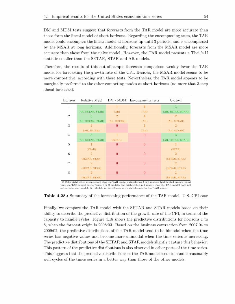
4.1 Empirical results for the United States economic time series 54
DM and MDM tests suggest that forecasts from the TAR model are more accurate than
those form the lineal model at short horizons. Regarding the encompassing tests, the TAR
model could encompass the linear model at horizons up until 3 periods, and is encompassed
by the MSAR at long horizons. Additionally, forecasts from the MSAR model are more
accurate than those from the naıve model. However, the TAR model presents a Theil’s U
statistic smaller than the SETAR, STAR and AR models.
Therefore, the results of this out-of-sample forecasts comparison weakly favor the TAR
model for forecasting the growth rate of the CPI. Besides, the MSAR model seems to be
more competitive, according with these tests. Nevertheless, the TAR model appears to be
marginally preferred to the other competing modes at short horizons (no more that 3-step
ahead forecasts).
Horizon Relative MSE DM - MDM Encompassing tests U-Theil
1 3 1 1 3
(AR, SETAR, STAR) (AR) (AR) (AR, SETAR, STAR)
2 3 2 1 2
(AR, SETAR, STAR) (AR, SETAR) (AR) (AR, SETAR)
3 2 0 1 2
(AR, SETAR) (AR) (AR, SETAR)
4 3 1 0 3
(AR, SETAR, STAR) (STAR) (AR, SETAR, STAR)
5 1 0 0 1
(STAR) (STAR)
6 2 0 0 2
(SETAR, STAR) (SETAR, STAR)
7 2 0 0 2
(SETAR, STAR) (SETAR, STAR)
8 2 0 0 2
(SETAR, STAR) (SETAR, STAR)
(1) Cells highlighted green report that the TAR model outperforms 3 or 4 models, highlighted orange report
that the TAR model outperforms 1 or 2 models, and highlighted red report that the TAR model does not
outperform any model. (2) Models in parenthesis are outperformed by the TAR model.
Table 4.28.: Summary of the forecasting performance of the TAR model. U.S. CPI case
Finally, we compare the TAR model with the SETAR and STAR models based on their
ability to describe the predictive distribution of the growth rate of the CPI, in terms of the
capacity to handle cycles. Figure 4.18 shows the predictive distributions for horizons 1 to
8, when the forecast origin is 2008:03. Based on the business contraction from 2007:04 to
2009:02, the predictive distributions of the TAR model tend to be bimodal when the time
series has negative values and become more unimodal when the time series is increasing.
The predictive distributions of the SETAR and STAR models slightly capture this behavior.
This pattern of the predictive distributions is also observed in other parts of the time series.
This suggests that the predictive distributions of the TAR model seem to handle reasonably
well cycles of the times series in a better way than those of the other models.

4.1 Empirical results for the United States economic time series 55
(a)
(b)
(c)
Figure 4.18.: 1 to 8-step predictive distributions of the change in the unemployment rate
series, for the (a) TAR, (b) SETAR and (c) STAR models. U.S. CPI case.

4.2 Empirical results for the Colombian economic time series 56
As a global summary for the U.S. case, this empirical evaluation shows that forecasts from
the TAR model outperform forecasts from the competing models at different h-step ahead
horizons, for all the considered economic times series, although in general, the forecasting
performance of this model is not better than that of the MSAR model. According to all the
used evaluation criteria, the TAR model forecasts the unemployment rate better than the
other models, at forecasts horizons greater than 2 periods ahead, and also, it’s the model
with the best in-sample properties. Regarding the GDP, industrial production index and
the CPI time series, forecasts from the TAR model outperform forecasts from the other
models, only according the relative MSE and Theil’s U statistic and for horizons between
1 and 5 periods ahead. However, it prevails as the model with great in-sample properties.
It is also relevant to remark that the TAR model shows a shape changing characteristic
in the Bayesian predictive distributions of this model that may capture the cycles in the
economic time series.
4.2. Empirical results for the Colombian economic time series
4.2.1. Unemployment rate
Description of the data
The data consists on the change in the seasonally adjusted Colombian monthly unem-
ployment rate28 (the first difference of the time series) and, from 2002:02 to 2016:09 (189
observations), and the growth rate of the seasonally adjusted Colombian monthly ISE in-
dex data (the first difference of the logarithm of the time series) over the same period.
This period is chosen due to institutional constraints and the data is respectively obtained
from both the Central Bank of Colombia databases and the DANE. Nonetheless, this is
an interesting period to analyze because the Colombian economy began a recovery period,
with a modified macroeconomic policy, after the financial crisis of the late 90s.
In Figure 4.19 we observe that changes in the unemployment rate are less volatile since 2008
than at the beginning of the analyzed period, while the ISE index allows us to identify the
recovery of the Colombian economy in 2002 after the crisis of the late 90s and the posterior
contraction in 2009 because of the U.S. financial crisis of 2007. For comparison, we use the
business cycle determined by Alfonso et al. (2012), which are the grid areas that denote
the contractions from peak to trough.
28 The Colombian monthly unemployment rate, retrieved from the Central Bank of Colombia, has seasonal
patterns, thus this time series was seasonally adjusted using the X13-ARIMA program of the U.S.
Census Bureau of the U.S. Department of commerce.

4.2 Empirical results for the Colombian economic time series 57
Figure 4.19.: (a) Time plot of the change in the the Colombian monthly unemployment
rate and (b) time plot of growth rate of Colombian ISE monthly index.
Then, we use as the training subsample all the observations from 2001:02 to 2011:12 (131
observations). The remaining observations are reserved for the out-of-sample forecasting
comparison. The selection of the forecast horizon for monthly time series is based on the
literature review. Then, a sequence of 1 to 12-step ahead forecasts are generated from
the forecast origin 2011:12. After that, the forecast origin is moved one period ahead and
forecasts are calculated again. This procedure is repeated until we compute 53 1-step
ahead forecasts, 57 2-step ahead forecasts, and so on until 46 12-step ahead forecasts.
Estimation of models
Based on the estimation procedure in Appendix F, Table 4.29 shows a summary of the
model adequacy of the analyzed models. Globally, it is observed that the TAR and SETAR
models exhibit a reasonable in-sample fit, compared with the other models.
Model adequacy AR TAR SETAR STAR MSAR
White noise 1 1 1 1 2
Model specification 2 1 1 2 3
Homoscedasticity 3 3 3 3 3Cells with number 1 and highlighted green represent good adequacy, 2 and highlighted orange
represent regular adequacy, and 3 and highlighted red represent bad adequacy.
Table 4.29.: Model adequacy. Colombian unemployment rate case.
Forecasting evaluation
Table 4.30 shows the HP unbiased test and Ljung-Box’s Q correlation test. In general, at
the 10% significance level, forecasts errors for all the models are unbiased, and only the
TAR, SETAR and STAR shows uncorrelated forecasts errors at horizons greater than 7, 4
and 1 periods, respectively.
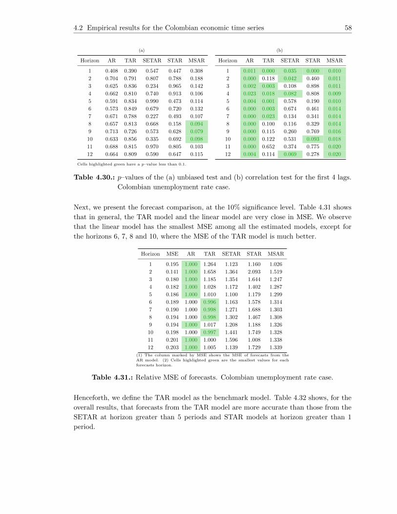
4.2 Empirical results for the Colombian economic time series 58
(a)
Horizon AR TAR SETAR STAR MSAR
1 0.408 0.390 0.547 0.447 0.308
2 0.704 0.791 0.807 0.788 0.188
3 0.625 0.836 0.234 0.965 0.142
4 0.662 0.810 0.740 0.913 0.106
5 0.591 0.834 0.990 0.473 0.114
6 0.573 0.849 0.679 0.720 0.132
7 0.671 0.788 0.227 0.493 0.107
8 0.657 0.813 0.668 0.158 0.094
9 0.713 0.726 0.573 0.628 0.079
10 0.633 0.856 0.335 0.692 0.098
11 0.688 0.815 0.970 0.805 0.103
12 0.664 0.809 0.590 0.647 0.115
(b)
Horizon AR TAR SETAR STAR MSAR
1 0.011 0.000 0.035 0.000 0.010
2 0.000 0.118 0.042 0.460 0.011
3 0.002 0.003 0.108 0.898 0.011
4 0.023 0.018 0.082 0.808 0.009
5 0.004 0.001 0.578 0.190 0.010
6 0.000 0.003 0.674 0.461 0.014
7 0.000 0.023 0.134 0.341 0.014
8 0.000 0.100 0.116 0.329 0.014
9 0.000 0.115 0.260 0.769 0.016
10 0.000 0.122 0.531 0.093 0.018
11 0.000 0.652 0.374 0.775 0.020
12 0.004 0.114 0.069 0.278 0.020
Cells highlighted green have a p–value less than 0.1.
Table 4.30.: p–values of the (a) unbiased test and (b) correlation test for the first 4 lags.
Colombian unemployment rate case.
Next, we present the forecast comparison, at the 10% significance level. Table 4.31 shows
that in general, the TAR model and the linear model are very close in MSE. We observe
that the linear model has the smallest MSE among all the estimated models, except for
the horizons 6, 7, 8 and 10, where the MSE of the TAR model is much better.
Horizon MSE AR TAR SETAR STAR MSAR
1 0.195 1.000 1.264 1.123 1.160 1.026
2 0.141 1.000 1.658 1.364 2.093 1.519
3 0.180 1.000 1.185 1.354 1.644 1.247
4 0.182 1.000 1.028 1.172 1.402 1.287
5 0.186 1.000 1.010 1.100 1.179 1.299
6 0.189 1.000 0.996 1.163 1.578 1.314
7 0.190 1.000 0.998 1.271 1.688 1.303
8 0.194 1.000 0.998 1.302 1.467 1.308
9 0.194 1.000 1.017 1.208 1.188 1.326
10 0.198 1.000 0.997 1.441 1.749 1.328
11 0.201 1.000 1.000 1.596 1.008 1.338
12 0.203 1.000 1.005 1.139 1.729 1.339
(1) The column marked by MSE shows the MSE of forecasts from the
AR model. (2) Cells highlighted green are the smallest values for each
forecasts horizon.
Table 4.31.: Relative MSE of forecasts. Colombian unemployment rate case.
Henceforth, we define the TAR model as the benchmark model. Table 4.32 shows, for the
overall results, that forecasts from the TAR model are more accurate than those from the
SETAR at horizon greater than 5 periods and STAR models at horizon greater than 1
period.
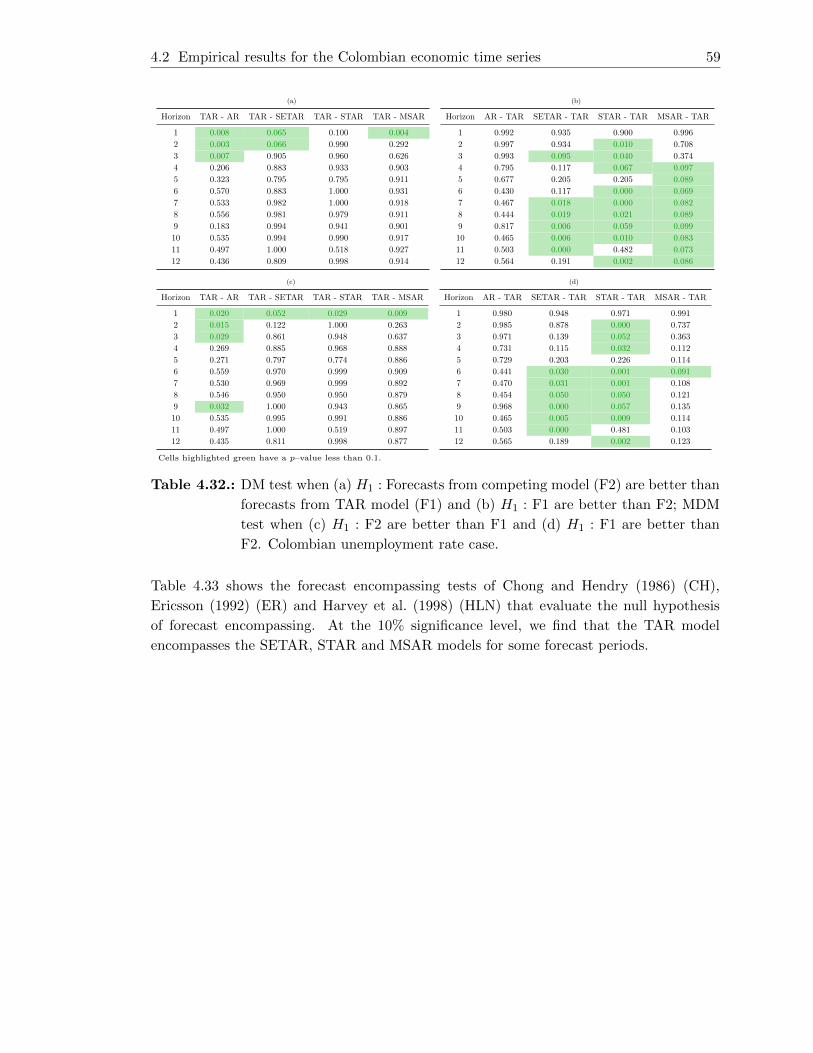
4.2 Empirical results for the Colombian economic time series 59
(a)
Horizon TAR - AR TAR - SETAR TAR - STAR TAR - MSAR
1 0.008 0.065 0.100 0.004
2 0.003 0.066 0.990 0.292
3 0.007 0.905 0.960 0.626
4 0.206 0.883 0.933 0.903
5 0.323 0.795 0.795 0.911
6 0.570 0.883 1.000 0.931
7 0.533 0.982 1.000 0.918
8 0.556 0.981 0.979 0.911
9 0.183 0.994 0.941 0.901
10 0.535 0.994 0.990 0.917
11 0.497 1.000 0.518 0.927
12 0.436 0.809 0.998 0.914
(b)
Horizon AR - TAR SETAR - TAR STAR - TAR MSAR - TAR
1 0.992 0.935 0.900 0.996
2 0.997 0.934 0.010 0.708
3 0.993 0.095 0.040 0.374
4 0.795 0.117 0.067 0.097
5 0.677 0.205 0.205 0.089
6 0.430 0.117 0.000 0.069
7 0.467 0.018 0.000 0.082
8 0.444 0.019 0.021 0.089
9 0.817 0.006 0.059 0.099
10 0.465 0.006 0.010 0.083
11 0.503 0.000 0.482 0.073
12 0.564 0.191 0.002 0.086
(c)
Horizon TAR - AR TAR - SETAR TAR - STAR TAR - MSAR
1 0.020 0.052 0.029 0.009
2 0.015 0.122 1.000 0.263
3 0.029 0.861 0.948 0.637
4 0.269 0.885 0.968 0.888
5 0.271 0.797 0.774 0.886
6 0.559 0.970 0.999 0.909
7 0.530 0.969 0.999 0.892
8 0.546 0.950 0.950 0.879
9 0.032 1.000 0.943 0.865
10 0.535 0.995 0.991 0.886
11 0.497 1.000 0.519 0.897
12 0.435 0.811 0.998 0.877
(d)
Horizon AR - TAR SETAR - TAR STAR - TAR MSAR - TAR
1 0.980 0.948 0.971 0.991
2 0.985 0.878 0.000 0.737
3 0.971 0.139 0.052 0.363
4 0.731 0.115 0.032 0.112
5 0.729 0.203 0.226 0.114
6 0.441 0.030 0.001 0.091
7 0.470 0.031 0.001 0.108
8 0.454 0.050 0.050 0.121
9 0.968 0.000 0.057 0.135
10 0.465 0.005 0.009 0.114
11 0.503 0.000 0.481 0.103
12 0.565 0.189 0.002 0.123
Cells highlighted green have a p–value less than 0.1.
Table 4.32.: DM test when (a) H1 : Forecasts from competing model (F2) are better than
forecasts from TAR model (F1) and (b) H1 : F1 are better than F2; MDM
test when (c) H1 : F2 are better than F1 and (d) H1 : F1 are better than
F2. Colombian unemployment rate case.
Table 4.33 shows the forecast encompassing tests of Chong and Hendry (1986) (CH),
Ericsson (1992) (ER) and Harvey et al. (1998) (HLN) that evaluate the null hypothesis
of forecast encompassing. At the 10% significance level, we find that the TAR model
encompasses the SETAR, STAR and MSAR models for some forecast periods.

4.2 Empirical results for the Colombian economic time series 60
(a)
Horizon TAR - AR TAR - SETAR TAR - STAR TAR - MSAR
1 0.136 0.099 0.017 0.060
2 0.000 0.573 0.233 0.615
3 0.922 0.199 0.426 0.629
4 0.319 0.511 0.705 0.578
5 0.959 0.563 0.045 0.630
6 0.140 0.364 0.045 0.640
7 0.272 0.817 0.020 0.540
8 0.355 0.610 0.711 0.557
9 0.707 0.510 0.119 0.538
10 0.737 0.292 0.269 0.534
11 0.256 0.016 0.010 0.624
12 0.930 0.814 0.032 0.593
(b)
Horizon AR - TAR SETAR - TAR STAR - TAR MSAR - TAR
1 0.000 0.000 0.000 0.000
2 0.000 0.000 0.000 0.000
3 0.000 0.000 0.000 0.000
4 0.880 0.319 0.300 0.069
5 0.765 0.742 0.544 0.076
6 0.484 0.143 0.737 0.281
7 0.524 0.330 0.453 0.193
8 0.431 0.715 0.042 0.075
9 0.876 0.139 0.211 0.020
10 0.665 0.565 0.516 0.230
11 0.695 0.812 0.804 0.085
12 0.794 0.222 0.634 0.085
(c)
Horizon TAR - AR TAR - SETAR TAR - STAR TAR - MSAR
1 0.000 0.000 0.348 0.000
2 0.000 0.002 0.745 0.018
3 0.000 0.592 0.572 0.098
4 0.164 0.304 0.033 0.413
5 0.214 0.399 0.020 0.516
6 0.660 0.349 0.571 0.576
7 0.630 0.736 0.688 0.479
8 0.607 0.671 0.046 0.525
9 0.092 0.755 0.336 0.454
10 0.798 0.284 0.010 0.506
11 0.683 0.027 0.050 0.569
12 0.557 0.718 0.014 0.541
(d)
Horizon AR - TAR SETAR - TAR STAR - TAR MSAR - TAR
1 0.004 0.921 0.000 0.000
2 0.000 0.804 0.000 0.226
3 0.001 0.003 0.000 0.021
4 0.790 0.000 0.000 0.000
5 0.721 0.016 0.000 0.000
6 0.429 0.000 0.000 0.000
7 0.516 0.000 0.000 0.000
8 0.426 0.000 0.000 0.000
9 0.875 0.000 0.000 0.000
10 0.665 0.000 0.008 0.000
11 0.695 0.000 0.000 0.000
12 0.794 0.016 0.595 0.000
(e)
Horizon TAR - AR TAR - SETAR TAR - STAR TAR - MSAR
1 0.003 0.008 0.029 0.003
2 0.003 0.007 0.201 0.037
3 0.003 0.302 0.371 0.059
4 0.086 0.164 0.280 0.200
5 0.090 0.218 0.020 0.250
6 0.329 0.161 0.975 0.282
7 0.317 0.371 0.717 0.229
8 0.306 0.664 0.344 0.250
9 0.052 0.625 0.043 0.213
10 0.399 0.862 0.817 0.243
11 0.342 0.979 0.026 0.275
12 0.283 0.352 0.954 0.260
(f)
Horizon AR - TAR SETAR - TAR STAR - TAR MSAR - TAR
1 0.973 0.460 0.693 0.994
2 0.998 0.597 0.000 0.110
3 0.984 0.001 0.001 0.027
4 0.605 0.000 0.003 0.011
5 0.365 0.004 0.001 0.010
6 0.217 0.009 0.000 0.007
7 0.255 0.001 0.000 0.010
8 0.208 0.002 0.000 0.013
9 0.563 0.000 0.000 0.013
10 0.334 0.000 0.001 0.010
11 0.347 0.000 0.006 0.010
12 0.396 0.050 0.000 0.012
Cells highlighted green have a p–value less than 0.1.
Table 4.33.: CH test when (a) H0 : F1 encompasses F2 and (b) H0: F2 encompasses F1;
ER test when (c) H0 : F1 encompasses F2 and (d) H0: F2 encompasses F1;
HLN test when (e) H0 : F1 encompasses F2 and (f) H0: F2 encompasses F1.
Colombian unemployment rate case.
Table 4.34 shows that forecasts from all models are more accurate than those from the
naıve model, where the AR and TAR model have the smallest value of the test.

4.2 Empirical results for the Colombian economic time series 61
Horizon AR TAR SETAR STAR MSAR
1 0.629 0.707 0.667 0.678 0.637
2 0.532 0.685 0.621 0.770 0.656
3 0.596 0.649 0.693 0.764 0.665
4 0.594 0.602 0.643 0.704 0.674
5 0.596 0.599 0.625 0.647 0.679
6 0.596 0.595 0.643 0.749 0.683
7 0.595 0.594 0.671 0.773 0.679
8 0.596 0.595 0.680 0.722 0.681
9 0.592 0.597 0.651 0.646 0.682
10 0.595 0.594 0.714 0.787 0.686
11 0.594 0.594 0.751 0.597 0.687
12 0.594 0.596 0.634 0.782 0.688Cells highlighted green represent the lowest value for each forecast horizon.
Table 4.34.: Theil’s U statistic. Colombian unemployment rate case.
As a summary, it is observed that forecasts errors for all the models are unbiased, and
only the TAR, SETAR and STAR shows uncorrelated forecasts errors at different horizons.
Additionally, Table 4.35 indicates a satisfactory performance of the TAR model. According
to the relative MSE of forecasts, we observe that the linear model has the smallest MSE
at short horizons, and the TAR model has better MSE at middle horizons. The DM and
MDM test suggest that forecasts from the TAR model are more accurate than those from
the SETAR and STAR models. Besides, the TAR model encompasses the SETAR, STAR
and MSAR models for some horizons. Following the Theil’s U statistic, forecasts from AR
and TAR models are more accurate from those from the naıve model.
Therefore, from this out-of-sample forecasts comparison, we can conclude that the TAR
model could forecasts the change in the unemployment rate with a satisfactory perfor-
mance, given that of the alternatives, the TAR model appears to be marginally preferred
to the competing modes.
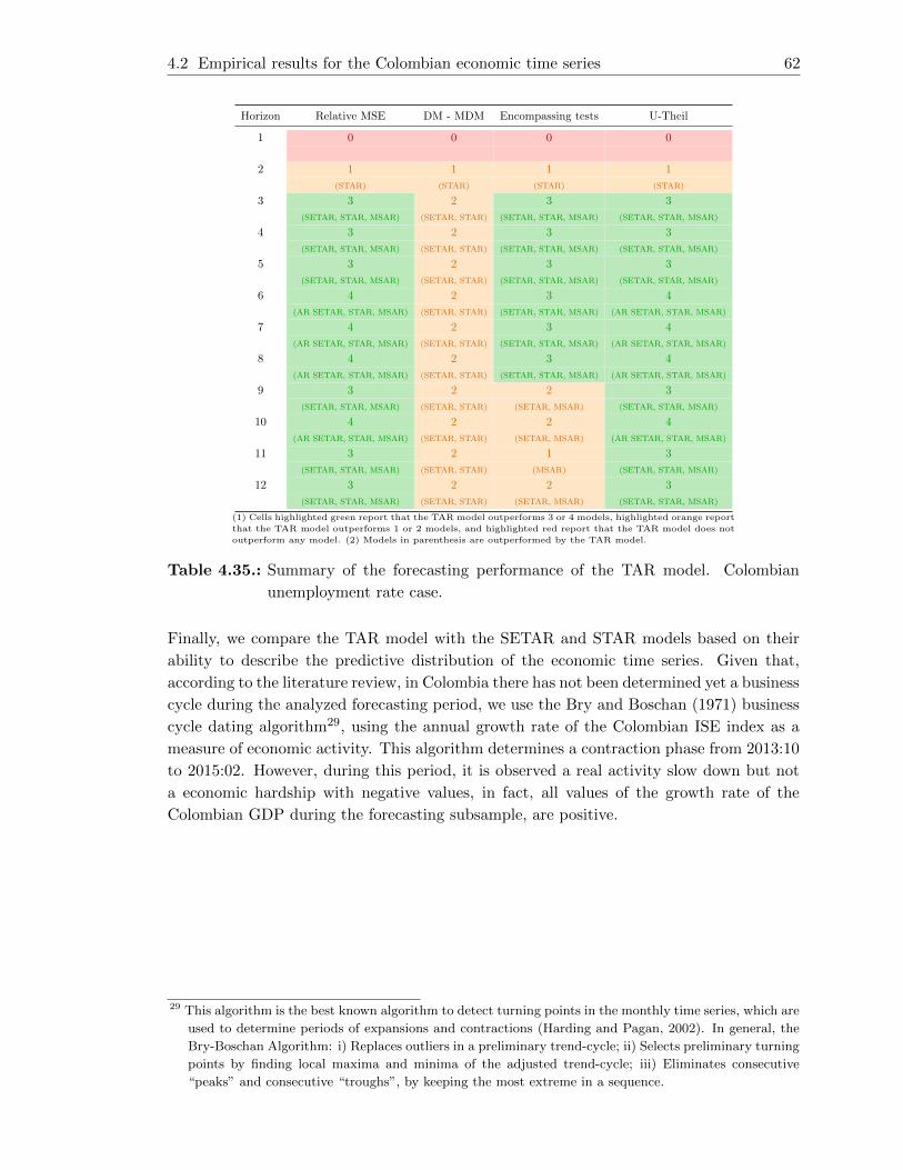
4.2 Empirical results for the Colombian economic time series 62
Horizon Relative MSE DM - MDM Encompassing tests U-Theil
1 0 0 0 0
2 1 1 1 1
(STAR) (STAR) (STAR) (STAR)
3 3 2 3 3
(SETAR, STAR, MSAR) (SETAR, STAR) (SETAR, STAR, MSAR) (SETAR, STAR, MSAR)
4 3 2 3 3
(SETAR, STAR, MSAR) (SETAR, STAR) (SETAR, STAR, MSAR) (SETAR, STAR, MSAR)
5 3 2 3 3
(SETAR, STAR, MSAR) (SETAR, STAR) (SETAR, STAR, MSAR) (SETAR, STAR, MSAR)
6 4 2 3 4
(AR SETAR, STAR, MSAR) (SETAR, STAR) (SETAR, STAR, MSAR) (AR SETAR, STAR, MSAR)
7 4 2 3 4
(AR SETAR, STAR, MSAR) (SETAR, STAR) (SETAR, STAR, MSAR) (AR SETAR, STAR, MSAR)
8 4 2 3 4
(AR SETAR, STAR, MSAR) (SETAR, STAR) (SETAR, STAR, MSAR) (AR SETAR, STAR, MSAR)
9 3 2 2 3
(SETAR, STAR, MSAR) (SETAR, STAR) (SETAR, MSAR) (SETAR, STAR, MSAR)
10 4 2 2 4
(AR SETAR, STAR, MSAR) (SETAR, STAR) (SETAR, MSAR) (AR SETAR, STAR, MSAR)
11 3 2 1 3
(SETAR, STAR, MSAR) (SETAR, STAR) (MSAR) (SETAR, STAR, MSAR)
12 3 2 2 3
(SETAR, STAR, MSAR) (SETAR, STAR) (SETAR, MSAR) (SETAR, STAR, MSAR)
(1) Cells highlighted green report that the TAR model outperforms 3 or 4 models, highlighted orange report
that the TAR model outperforms 1 or 2 models, and highlighted red report that the TAR model does not
outperform any model. (2) Models in parenthesis are outperformed by the TAR model.
Table 4.35.: Summary of the forecasting performance of the TAR model. Colombian
unemployment rate case.
Finally, we compare the TAR model with the SETAR and STAR models based on their
ability to describe the predictive distribution of the economic time series. Given that,
according to the literature review, in Colombia there has not been determined yet a business
cycle during the analyzed forecasting period, we use the Bry and Boschan (1971) business
cycle dating algorithm29, using the annual growth rate of the Colombian ISE index as a
measure of economic activity. This algorithm determines a contraction phase from 2013:10
to 2015:02. However, during this period, it is observed a real activity slow down but not
a economic hardship with negative values, in fact, all values of the growth rate of the
Colombian GDP during the forecasting subsample, are positive.
29 This algorithm is the best known algorithm to detect turning points in the monthly time series, which are
used to determine periods of expansions and contractions (Harding and Pagan, 2002). In general, the
Bry-Boschan Algorithm: i) Replaces outliers in a preliminary trend-cycle; ii) Selects preliminary turning
points by finding local maxima and minima of the adjusted trend-cycle; iii) Eliminates consecutive
“peaks” and consecutive “troughs”, by keeping the most extreme in a sequence.

4.2 Empirical results for the Colombian economic time series 63
(a)
(b)
(c)
Figure 4.20.: 1 to 8-step predictive distributions of the change in the unemployment rate
series, for the (a) TAR, (b) SETAR and (c) STAR models. Colombian
unemployment rate case.

4.2 Empirical results for the Colombian economic time series 64
Figure 4.20 shows the predictive distributions for horizons 1 to 8, when the forecast origin
is 2013:08. The predictive distributions of the TAR model tend to be unimodal when
the time series is ascending to a peak (negative increments of the unemployment rate),
although it does not capture the bimodal shape in unstable periods. That behavior could
be explained in the sense that, there is no a strong contraction phase in the Colombian
real activity during the forecasting period, as it was mentioned above. The predictive
distributions of the SETAR and STAR models have the same performance. This pattern
of the predictive distributions is also observed in other parts of the time series.
4.2.2. Gross domestic product
Description of the data
We analyze, as a proxy of the GDP, the annual growth rate of the seasonally adjusted
Colombian monthly indicator of the real economic activity ISE, from 2003:01 to 2016:09
(165 observations), which was retrieved from the DANE. As the threshold value, we use the
term spread defined in Section 3.2 over the same period, that is, the difference between the
ten-year Treasury bonds (TES) as the long-term government bond rate, and the inter-bank
interest rate as the overnight rate. Both series were retrieved from the Central Bank of
Colombia.
For the forecast comparison, we denote Xt = [log(ISEt)− log(ISEt−12)] ∗ 100 as the
annual growth rate of the ISE, and Zt, the spread term defined above. Both series are
plotted in Figure 4.21 that shows a similar behavior during contractions periods of these
series. The shading areas denote the business cycle contractions from peak to trough based
on Alfonso et al. (2012).
Figure 4.21.: (a) Time plot of the annual growth rate of Colombian GDP and (b) time
plot of Colombian term spread.
We use as the training subsample, the data until 2012:06 (114 observations). The remain-
ing observations are reserved for the out-of-sample forecasting evaluation. By using the
procedure mentioned at the begining of this Chapter, a sequence of 1 to 12-step ahead
forecasts are generated until we compute 51 1-step ahead forecasts, down to 40 12-step
ahead forecast.

4.2 Empirical results for the Colombian economic time series 65
Estimation of models
Based on results in Appendix G, Table 4.36 shows that globally, the STAR model presents
the best reasonable in-sample fit, followed by the TAR, SETAR and AR models.
Model adequacy AR TAR SETAR STAR MSAR
White noise 2 2 2 1 1
Model specification 1 1 1 1 3
Homoscedasticity 1 1 1 1 2Cells with number 1 and highlighted green represent good adequacy, 2 and highlighted orange
represent regular adequacy, and 3 and highlighted red represent bad adequacy.
Table 4.36.: Model adequacy. Colombian GDP case.
Forecasting evaluation
Table 4.37 shows the HP unbiased test and Ljung-Box’s Q correlation test. Globally, at the
10% significance level, only forecasts errors of the SETAR model are unbiased, and only
the SETAR and STAR exhibit uncorrelated forecasts errors at some forescasts peroiods.
(a)
Horizon AR TAR SETAR STAR MSAR
1 0.076 0.007 0.611 0.048 0.000
2 0.017 0.001 0.456 0.041 0.000
3 0.004 0.000 0.105 0.028 0.000
4 0.004 0.000 0.306 0.009 0.000
5 0.002 0.000 0.686 0.016 0.000
6 0.001 0.000 0.848 0.007 0.000
7 0.001 0.000 0.909 0.001 0.000
8 0.001 0.000 0.955 0.001 0.000
9 0.001 0.000 0.997 0.001 0.000
10 0.001 0.000 0.900 0.001 0.000
11 0.001 0.000 0.730 0.000 0.000
12 0.001 0.000 0.862 0.000 0.000
(b)
Horizon AR TAR SETAR STAR MSAR
1 0.000 0.000 0.000 0.000 0.000
2 0.000 0.000 0.000 0.000 0.000
3 0.000 0.000 0.000 0.009 0.000
4 0.000 0.000 0.000 0.205 0.000
5 0.000 0.000 0.000 0.796 0.000
6 0.000 0.000 0.001 0.951 0.000
7 0.000 0.000 0.021 0.529 0.000
8 0.000 0.002 0.128 0.629 0.000
9 0.000 0.010 0.123 0.257 0.000
10 0.000 0.039 0.469 0.056 0.000
11 0.000 0.068 0.579 0.000 0.000
12 0.000 0.076 0.701 0.002 0.000
Cells highlighted green have a p–value less than 0.1.
Table 4.37.: p–values of the (a) unbiased test and (b) correlation test for the first 4 lags.
Colombian GDP case.
Now, we present the forecast comparison, also at the 10% significance level. Table 4.38
shows in general that the AR model has the smallest MSE among all the estimated models,
follow by the MSAR and TAR models.

4.2 Empirical results for the Colombian economic time series 66
Horizon MSE AR TAR SETAR STAR MSAR
1 0.893 1.000 1.061 1.118 0.984 2.850
2 1.133 1.000 1.257 1.528 1.430 2.699
3 1.242 1.000 1.311 2.082 2.142 2.418
4 1.679 1.000 1.256 2.549 2.148 1.850
5 1.993 1.000 1.229 2.289 2.157 1.592
6 2.239 1.000 1.270 1.767 1.383 1.427
7 2.465 1.000 1.250 2.442 1.367 1.308
8 2.805 1.000 1.237 2.638 1.574 1.172
9 3.047 1.000 1.213 2.912 1.517 1.066
10 3.201 1.000 1.169 2.861 1.658 1.004
11 3.371 1.000 1.138 3.011 1.923 0.976
12 3.490 1.000 1.141 3.374 1.795 0.962
(1) The column marked by MSE shows the MSE of forecasts from the
AR model. (2) Cells highlighted green are the smallest values for each
forecasts horizon.
Table 4.38.: Relative MSE of forecasts. Colombian GDP case.
Hereafter, we define the TAR model as the benchmark model. Table 4.39 shows that for
the overall comparison, forecasts from the TAR model are more accurate than those from
the SETAR and STAR models at long horizons, and more accurate than those from the
MSAR model at short horizons, although forecasts from the linear model are more accurate
than those from the TAR model, in general.
(a)
Horizon TAR - AR TAR - SETAR TAR - STAR TAR - MSAR
1 0.168 0.684 0.283 1.000
2 0.003 0.878 0.804 1.000
3 0.002 0.930 0.990 1.000
4 0.020 0.995 0.998 0.967
5 0.007 0.996 0.994 0.943
6 0.015 0.770 0.637 0.678
7 0.045 0.967 0.629 0.561
8 0.042 0.977 0.883 0.428
9 0.064 0.985 0.809 0.342
10 0.131 0.983 0.946 0.327
11 0.157 0.993 1.000 0.328
12 0.137 0.994 0.999 0.315
(b)
Horizon AR - TAR SETAR - TAR STAR - TAR MSAR - TAR
1 0.832 0.316 0.717 0.000
2 0.997 0.122 0.196 0.000
3 0.998 0.070 0.010 0.000
4 0.980 0.005 0.002 0.033
5 0.993 0.004 0.006 0.057
6 0.985 0.230 0.363 0.322
7 0.955 0.033 0.371 0.439
8 0.958 0.023 0.117 0.572
9 0.936 0.015 0.191 0.658
10 0.869 0.017 0.054 0.673
11 0.843 0.007 0.000 0.672
12 0.863 0.006 0.001 0.685
(c)
Horizon TAR - AR TAR - SETAR TAR - STAR TAR - MSAR
1 0.166 0.686 0.281 1.000
2 0.003 0.880 0.806 1.000
3 0.001 0.932 0.990 0.999
4 0.019 0.995 0.998 0.929
5 0.006 0.996 0.995 0.944
6 0.030 0.715 0.631 0.641
7 0.077 0.923 0.608 0.548
8 0.086 0.952 0.846 0.446
9 0.132 0.961 0.753 0.384
10 0.186 0.960 0.872 0.370
11 0.221 0.975 0.999 0.369
12 0.198 0.982 1.000 0.363
(d)
Horizon AR - TAR SETAR - TAR STAR - TAR MSAR - TAR
1 0.834 0.314 0.719 0.000
2 0.997 0.120 0.194 0.000
3 0.999 0.068 0.010 0.001
4 0.981 0.005 0.002 0.071
5 0.994 0.004 0.005 0.056
6 0.970 0.286 0.369 0.359
7 0.923 0.077 0.392 0.452
8 0.914 0.048 0.154 0.554
9 0.868 0.039 0.247 0.616
10 0.814 0.040 0.128 0.630
11 0.779 0.025 0.001 0.631
12 0.802 0.018 0.000 0.637
Cells highlighted green have a p–value less than 0.1.
Table 4.39.: DM test when (a) H1 : Forecasts from competing model (F2) are better than
forecasts from TAR model (F1) and (b) H1 : F1 are better than F2; MDM
test when (c) H1 : F2 are better than F1 and (d) H1 : F1 are better than
F2. Colombian GDP case.

4.2 Empirical results for the Colombian economic time series 67
Table 4.40 shows that the linear model encompasses the TAR model at long horizons, but
under the ER and HLN tests, the TAR model encompasses the SETAR and STAR models
at horizons greater than 5 and 8 periods respectively, while the TAR and MSAR model do
not encompass each other.
(a)
Horizon TAR - AR TAR - SETAR TAR - STAR TAR - MSAR
1 0.011 0.011 0.020 0.361
2 0.007 0.015 0.011 0.009
3 0.001 0.006 0.001 0.021
4 0.000 0.000 0.000 0.274
5 0.000 0.000 0.000 0.287
6 0.070 0.059 0.106 0.028
7 0.063 0.037 0.136 0.332
8 0.048 0.024 0.097 0.339
9 0.047 0.009 0.080 0.325
10 0.049 0.013 0.066 0.354
11 0.045 0.005 0.054 0.383
12 0.041 0.002 0.058 0.371
(b)
Horizon AR - TAR SETAR - TAR STAR - TAR MSAR - TAR
1 0.058 0.345 0.047 0.000
2 0.018 0.186 0.024 0.000
3 0.007 0.052 0.029 0.000
4 0.004 0.218 0.008 0.000
5 0.002 0.530 0.015 0.000
6 0.118 0.804 0.085 0.000
7 0.127 0.855 0.016 0.000
8 0.105 0.887 0.013 0.000
9 0.107 0.928 0.028 0.000
10 0.117 0.995 0.039 0.000
11 0.111 0.800 0.015 0.000
12 0.101 0.906 0.017 0.000
(c)
Horizon TAR - AR TAR - SETAR TAR - STAR TAR - MSAR
1 0.070 0.140 0.033 0.016
2 0.000 0.004 0.084 0.896
3 0.000 0.115 0.681 0.014
4 0.000 0.288 0.532 0.006
5 0.000 0.095 0.505 0.000
6 0.000 0.128 0.010 0.000
7 0.007 0.259 0.017 0.001
8 0.008 0.340 0.044 0.000
9 0.014 0.541 0.132 0.001
10 0.058 0.477 0.358 0.000
11 0.068 0.876 0.934 0.001
12 0.042 0.993 0.672 0.001
(d)
Horizon AR - TAR SETAR - TAR STAR - TAR MSAR - TAR
1 0.951 0.013 0.333 0.000
2 0.001 0.000 0.000 0.000
3 0.058 0.000 0.000 0.000
4 0.136 0.000 0.000 0.000
5 0.079 0.000 0.000 0.000
6 0.114 0.003 0.001 0.000
7 0.222 0.000 0.002 0.000
8 0.233 0.000 0.000 0.002
9 0.298 0.000 0.001 0.008
10 0.508 0.000 0.000 0.007
11 0.625 0.000 0.000 0.009
12 0.594 0.000 0.000 0.016
(e)
Horizon TAR - AR TAR - SETAR TAR - STAR TAR - MSAR
1 0.033 0.048 0.027 0.994
2 0.001 0.003 0.046 0.448
3 0.000 0.056 0.339 0.057
4 0.006 0.149 0.268 0.044
5 0.001 0.071 0.247 0.004
6 0.003 0.089 0.004 0.013
7 0.014 0.134 0.000 0.006
8 0.012 0.180 0.003 0.004
9 0.023 0.261 0.038 0.001
10 0.059 0.225 0.162 0.000
11 0.071 0.437 0.533 0.001
12 0.056 0.504 0.335 0.001
(f)
Horizon AR - TAR SETAR - TAR STAR - TAR MSAR - TAR
1 0.525 0.036 0.166 0.000
2 0.986 0.002 0.003 0.000
3 0.974 0.001 0.000 0.000
4 0.907 0.000 0.000 0.002
5 0.946 0.000 0.000 0.000
6 0.931 0.002 0.028 0.017
7 0.870 0.000 0.025 0.019
8 0.868 0.000 0.004 0.031
9 0.832 0.001 0.008 0.056
10 0.732 0.001 0.001 0.045
11 0.678 0.001 0.000 0.042
12 0.691 0.002 0.000 0.051
Cells highlighted green have a p–value less than 0.1.
Table 4.40.: CH test when (a) H0 : F1 encompasses F2 and (b) H0: F2 encompasses F1;
ER test when (c) H0 : F1 encompasses F2 and (d) H0: F2 encompasses F1;
HLN test when (e) H0 : F1 encompasses F2 and (f) H0: F2 encompasses F1.
Colombian GDP case.
Table 4.41 shows that only at horizons of 1 period, forecasts from all models, except the
MSAR model, are more accurate than those from the naıve model. Globally, the AR model
has the smallest value of the test, and the TAR model has the second-smallest value of the
test at horizons up until 7 periods.

4.2 Empirical results for the Colombian economic time series 68
Horizon AR TAR SETAR STAR MSAR
1 0.935 0.963 0.989 0.928 1.579
2 1.063 1.192 1.314 1.271 1.747
3 1.149 1.316 1.658 1.681 1.786
4 1.344 1.506 2.145 1.970 1.828
5 1.449 1.606 2.192 2.128 1.828
6 1.522 1.715 2.023 1.789 1.818
7 1.580 1.767 2.469 1.847 1.807
8 1.727 1.920 2.804 2.166 1.869
9 1.818 2.002 3.103 2.239 1.877
10 1.843 1.992 3.117 2.373 1.847
11 1.890 2.016 3.280 2.622 1.868
12 1.901 2.030 3.492 2.547 1.865Cells highlighted green represent the lowest value for each forecast horizon.
Table 4.41.: Theil’s U statistic. Colombian GDP case.
As a summary, it is observed that only the SETAR model has unbiased forecasts, and with
the STAR model, are the only models that present uncorrelated forecasts errors for some
forecast periods. Additionally, Table 4.42 let us observe a satisfactory performance of the
TAR model. According to the Relative MSE of forecast and the DM and MDM tests, the
TAR model has better MSE of forecasts than the SETAR, STAR and MSAR models, for
some horizons. Regarding the encompassing tests, only the TAR model encompasses the
SETAR model at all horizons, encompasses the STAR at long horizons and the MSAR at
short horizons. Additionally, forecasts from all models are not more accurate than those
from the naıve model.
Therefore, from this out-of-sample forecasts comparison, we can conclude that the TAR
model could forecasts the growth rate of the real GDP with a good performance, given that
of the alternatives, the TAR model appears to be marginally preferred to the competing
modes.

4.2 Empirical results for the Colombian economic time series 69
Horizon Relative MSE DM - MDM Encompassing tests U-Theil
1 2 1 1 2
(SETAR, MSAR) (MSAR) (MSAR) (SETAR, MSAR)
2 3 1 1 3
(SETAR, STAR, MSAR) (MSAR) (MSAR) (SETAR, STAR, MSAR)
3 3 3 1 3
(SETAR, STAR, MSAR) (SETAR, STAR, MSAR) (STAR) (SETAR, STAR, MSAR)
4 3 3 2 3
(SETAR, STAR, MSAR) (SETAR, STAR, MSAR) (SETAR, STAR) (SETAR, STAR, MSAR)
5 3 3 1 3
(SETAR, STAR, MSAR) (SETAR, STAR, MSAR) (STAR) (SETAR, STAR, MSAR)
6 3 0 1 3
(SETAR, STAR, MSAR) (SETAR) (SETAR, STAR, MSAR)
7 3 1 1 3
(SETAR, STAR, MSAR) (SETAR) (SETAR) (SETAR, STAR, MSAR)
8 2 1 1 2
(SETAR, STAR) (SETAR) (SETAR) (SETAR, STAR)
9 2 1 1 2
(SETAR, STAR) (SETAR) (SETAR) (SETAR, STAR)
10 2 1 2 2
(SETAR, STAR) (SETAR) (SETAR, STAR) (SETAR, STAR)
11 2 2 2 1
(SETAR, STAR) (SETAR, STAR) (SETAR, STAR) (SETAR)
12 2 2 2 1
(SETAR, STAR) (SETAR, STAR) (SETAR, STAR) (SETAR)
(1) Cells highlighted green report that the TAR model outperforms 3 or 4 models, highlighted orange report
that the TAR model outperforms 1 or 2 models, and highlighted red report that the TAR model does not
outperform any model. (2) Models in parenthesis are outperformed by the TAR model.
Table 4.42.: Summary of the forecasting performance of the TAR model. Colombian
GDP case.
Finally, we compare the TAR model with the SETAR and STAR models based on their
ability to describe the predictive distribution of the economic time series. As it was ob-
served in the Colombian unemployment rate case, the forecasting period of the time series
do not show a strong contraction phase (there are only positive values, that is, positive
growth rates of the GDP). Thus, the 1 to 8-step predictive distributions of the TAR,
SETAR and STAR models tend to be unimodal, capturing the stability of the time series.
4.2.3. Industrial production index
Description of the data
We analyze the seasonally adjusted Colombian biannual growth rate of Colombian indus-
trial production index, from 2003:01 to 2016:11 (167 observations), which was retrieved
from the DANE. As the threshold value, we use the term spread defined in Section 3.2
over the same period and mentioned above.
For the forecast comparison, we denote Xt =[log(Indprot)− log(Indprot−6)
]∗ 100 as
the annual growth rate of the Colombian industrial production index (indpro), and Zt,
the spread term. Both series are plotted in Figure 4.22 that shows a similar behavior
during contractions periods of these series. The shading areas denote the business cycle
contractions from peak to trough.

4.2 Empirical results for the Colombian economic time series 70
Figure 4.22.: (a) Time plot of the biannual growth rate of Colombian industrial produc-
tion index and (b) time plot of Colombian term spread.
We use as the training subsample, the data until 2012:06 (114 observations). The re-
maining observations are reserved for the out-of-sample forecasting evaluation. By using
the procedure mentioned in Section 4.1.1, a sequence of 1 to 12-step ahead forecasts are
generated until we compute 53 1-step ahead forecasts, down to 42 12-step ahead forecast.
Estimation of models
Based on results in Appendix H, Table 4.43 shows that, in general, the TAR and STAR
models present the best reasonable in-sample fit.
Model adequacy AR TAR SETAR STAR MSAR
White noise 2 1 2 1 1
Model specification 1 1 1 1 3
Homoscedasticity 1 1 1 1 1Cells with number 1 and highlighted green represent good adequacy, 2 and highlighted orange
represent regular adequacy, and 3 and highlighted red represent bad adequacy.
Table 4.43.: Model adequacy. Colombian indpro case.
Forecasting evaluation
Table 4.44 shows the HP unbiased test and Ljung-Box’s Q correlation test. At the 10% sig-
nificance level, forecasts errors of the SETAR model are unbiased, followed by the MSAR,
STAR and AR models for horizons up to 9. Regarding the Ljung Box test, in general,
the TAR, SETAR and STAR are the only models whose forecast errors do not have serial
correlation at horizons greater than 5 periods.

4.2 Empirical results for the Colombian economic time series 71
(a)
Horizon AR TAR SETAR STAR MSAR
1 0.814 0.045 0.706 0.865 0.613
2 0.657 0.047 0.898 0.673 0.776
3 0.546 0.014 0.946 0.752 0.940
4 0.465 0.002 0.882 0.257 0.872
5 0.537 0.000 0.916 0.549 0.783
6 0.444 0.000 0.423 0.178 0.598
7 0.259 0.000 0.240 0.153 0.347
8 0.165 0.000 0.159 0.019 0.238
9 0.083 0.002 0.207 0.036 0.152
10 0.028 0.003 0.117 0.024 0.073
11 0.020 0.002 0.354 0.042 0.056
12 0.013 0.010 0.466 0.169 0.047
(b)
Horizon AR TAR SETAR STAR MSAR
1 0.000 0.000 0.000 0.010 0.000
2 0.000 0.000 0.297 0.000 0.000
3 0.000 0.000 0.400 0.002 0.000
4 0.000 0.001 0.250 0.002 0.000
5 0.000 0.026 0.098 0.010 0.000
6 0.000 0.105 0.739 0.185 0.000
7 0.000 0.282 0.833 0.019 0.000
8 0.000 0.263 0.162 0.279 0.000
9 0.000 0.332 0.004 0.273 0.000
10 0.000 0.361 0.266 0.430 0.000
11 0.000 0.655 0.188 0.603 0.000
12 0.000 0.280 0.482 0.766 0.001
Cells highlighted green have a p–value less than 0.1.
Table 4.44.: p–values of the (a) unbiased test and (b) correlation test for the first 4 lags.
Colombian indpro case.
Now, we present the forecast comparison, also at the 10% significance level. Table 4.45
shows, for the overall comparison, the TAR model and the linear model are very close in
MSE, but the MSAR model is the one that has the smallest MSE. The TAR model has
the third-smallest MSE.
Horizon MSE AR TAR SETAR STAR MSAR
1 5.284 1.000 1.017 1.137 1.034 0.991
2 4.649 1.000 1.093 1.369 1.588 1.115
3 5.920 1.000 1.100 1.705 2.182 0.868
4 6.706 1.000 1.150 1.454 2.237 0.767
5 6.353 1.000 1.219 1.874 2.574 0.817
6 7.341 1.000 1.155 1.852 2.643 0.711
7 6.387 1.000 1.244 1.956 2.719 0.784
8 6.574 1.000 1.140 1.755 3.114 0.772
9 6.389 1.000 1.356 1.658 2.507 0.804
10 5.928 1.000 1.032 1.666 2.933 0.858
11 6.378 1.000 1.070 1.617 2.586 0.820
12 6.423 1.000 1.003 1.764 2.747 0.837
(1) The column marked by MSE shows the MSE of forecasts from the
AR model. (2) Cells highlighted green are the smallest values for each
forecasts horizon.
Table 4.45.: Relative MSE of forecasts. Colombian indpro case.
Hereafter, we define the TAR model as the benchmark model. Table 4.46 shows in general,
that forecasts from the TAR model are more accurate than those from the SETAR and
STAR at horizon greater than 2 and 1 periods respectively, but forecasts from the MSAR
models are more accurate than those from the TAR model at horizon over 3 and 9 periods.
We also find no significant difference between the TAR and AR MSE of the forecasts.
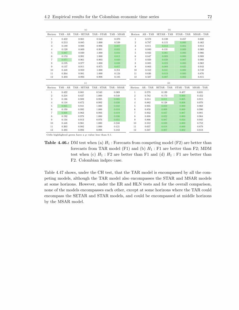
4.2 Empirical results for the Colombian economic time series 72
(a)
Horizon TAR - AR TAR - SETAR TAR - STAR TAR - MSAR
1 0.422 0.861 0.543 0.370
2 0.213 0.885 1.000 0.539
3 0.189 0.988 0.996 0.087
4 0.120 0.869 0.991 0.031
5 0.067 0.939 1.000 0.034
6 0.153 0.991 1.000 0.011
7 0.071 0.961 0.993 0.020
8 0.195 0.977 1.000 0.038
9 0.137 0.911 0.975 0.057
10 0.448 0.959 1.000 0.251
11 0.364 0.981 1.000 0.124
12 0.493 0.993 0.998 0.185
(b)
Horizon AR - TAR SETAR - TAR STAR - TAR MSAR - TAR
1 0.578 0.139 0.457 0.630
2 0.787 0.115 0.000 0.462
3 0.811 0.012 0.004 0.913
4 0.880 0.131 0.009 0.969
5 0.933 0.061 0.000 0.966
6 0.847 0.009 0.000 0.989
7 0.929 0.039 0.007 0.980
8 0.805 0.023 0.000 0.962
9 0.863 0.089 0.025 0.943
10 0.552 0.041 0.000 0.749
11 0.636 0.019 0.000 0.876
12 0.507 0.007 0.002 0.815
(c)
Horizon TAR - AR TAR - SETAR TAR - STAR TAR - MSAR
1 0.422 0.861 0.543 0.369
2 0.218 0.827 1.000 0.548
3 0.186 0.989 0.995 0.085
4 0.118 0.872 0.992 0.030
5 0.065 0.941 1.000 0.032
6 0.150 0.992 1.000 0.010
7 0.068 0.963 0.993 0.019
8 0.192 0.978 1.000 0.036
9 0.134 0.913 0.976 0.055
10 0.448 0.961 1.000 0.248
11 0.363 0.982 1.000 0.121
12 0.493 0.993 0.998 0.182
(d)
Horizon AR - TAR SETAR - TAR STAR - TAR MSAR - TAR
1 0.578 0.139 0.457 0.631
2 0.782 0.173 0.000 0.452
3 0.814 0.011 0.005 0.915
4 0.882 0.128 0.008 0.970
5 0.935 0.059 0.000 0.968
6 0.850 0.008 0.000 0.990
7 0.932 0.037 0.007 0.981
8 0.808 0.022 0.000 0.964
9 0.866 0.087 0.024 0.945
10 0.552 0.039 0.000 0.752
11 0.637 0.018 0.000 0.879
12 0.507 0.007 0.002 0.818
Cells highlighted green have a p–value less than 0.1.
Table 4.46.: DM test when (a) H1 : Forecasts from competing model (F2) are better than
forecasts from TAR model (F1) and (b) H1 : F1 are better than F2; MDM
test when (c) H1 : F2 are better than F1 and (d) H1 : F1 are better than
F2. Colombian indpro case.
Table 4.47 shows, under the CH test, that the TAR model is encompassed by all the com-
peting models, although the TAR model also encompasses the STAR and MSAR models
at some horizons. However, under the ER and HLN tests and for the overall comparison,
none of the models encompasses each other, except at some horizons where the TAR could
encompass the SETAR and STAR models, and could be encompassed at middle horizons
by the MSAR model.
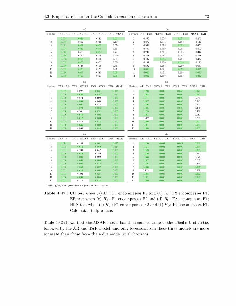
4.2 Empirical results for the Colombian economic time series 73
(a)
Horizon TAR - AR TAR - SETAR TAR - STAR TAR - MSAR
1 0.034 0.024 0.186 0.015
2 0.037 0.212 0.231 0.187
3 0.011 0.064 0.003 0.676
4 0.004 0.042 0.075 0.864
5 0.013 0.880 0.022 0.741
6 0.016 0.159 0.504 0.730
7 0.058 0.053 0.611 0.914
8 0.087 0.075 0.670 0.804
9 0.036 0.148 0.493 0.465
10 0.009 0.026 0.970 0.479
11 0.010 0.097 0.789 0.062
12 0.009 0.059 0.929 0.061
(b)
Horizon AR - TAR SETAR - TAR STAR - TAR MSAR - TAR
1 0.355 0.276 0.052 0.276
2 0.672 0.946 0.132 0.127
3 0.532 0.696 0.063 0.670
4 0.700 0.450 0.296 0.812
5 0.734 0.621 0.825 0.347
6 0.488 0.358 0.297 0.358
7 0.497 0.053 0.294 0.382
8 0.167 0.190 0.018 0.153
9 0.597 0.155 0.299 0.680
10 0.044 0.321 0.072 0.065
11 0.026 0.454 0.105 0.052
12 0.007 0.689 0.197 0.022
(c)
Horizon TAR - AR TAR - SETAR TAR - STAR TAR - MSAR
1 0.007 0.327 0.081 0.013
2 0.000 0.034 0.032 0.024
3 0.000 0.273 0.699 0.000
4 0.000 0.035 0.369 0.000
5 0.000 0.007 0.575 0.000
6 0.000 0.072 0.006 0.000
7 0.000 0.201 0.031 0.000
8 0.000 0.070 0.005 0.000
9 0.001 0.012 0.003 0.000
10 0.003 0.410 0.022 0.002
11 0.000 0.036 0.002 0.000
12 0.000 0.330 0.048 0.000
(d)
Horizon AR - TAR SETAR - TAR STAR - TAR MSAR - TAR
1 0.020 0.003 0.050 0.071
2 0.064 0.000 0.000 0.014
3 0.071 0.000 0.000 0.149
4 0.037 0.000 0.000 0.548
5 0.046 0.000 0.000 0.321
6 0.005 0.000 0.000 0.397
7 0.039 0.000 0.000 0.468
8 0.001 0.000 0.000 0.187
9 0.267 0.000 0.000 0.739
10 0.006 0.000 0.000 0.063
11 0.001 0.000 0.000 0.063
12 0.000 0.000 0.000 0.033
(e)
Horizon TAR - AR TAR - SETAR TAR - STAR TAR - MSAR
1 0.014 0.185 0.061 0.027
2 0.005 0.014 0.069 0.024
3 0.001 0.138 0.647 0.001
4 0.000 0.019 0.186 0.000
5 0.000 0.006 0.292 0.000
6 0.000 0.068 0.009 0.000
7 0.000 0.098 0.016 0.000
8 0.000 0.050 0.007 0.000
9 0.002 0.018 0.003 0.001
10 0.001 0.194 0.027 0.000
11 0.000 0.038 0.005 0.000
12 0.001 0.174 0.024 0.000
(f)
Horizon AR - TAR SETAR - TAR STAR - TAR MSAR - TAR
1 0.010 0.001 0.028 0.026
2 0.031 0.001 0.000 0.044
3 0.043 0.000 0.000 0.080
4 0.026 0.001 0.000 0.283
5 0.033 0.001 0.000 0.176
6 0.007 0.000 0.000 0.205
7 0.026 0.000 0.000 0.235
8 0.003 0.000 0.000 0.097
9 0.133 0.000 0.000 0.368
10 0.008 0.003 0.000 0.062
11 0.001 0.000 0.000 0.040
12 0.000 0.000 0.000 0.021
Cells highlighted green have a p–value less than 0.1.
Table 4.47.: CH test when (a) H0 : F1 encompasses F2 and (b) H0: F2 encompasses F1;
ER test when (c) H0 : F1 encompasses F2 and (d) H0: F2 encompasses F1;
HLN test when (e) H0 : F1 encompasses F2 and (f) H0: F2 encompasses F1.
Colombian indpro case.
Table 4.48 shows that the MSAR model has the smallest value of the Theil’s U statistic,
followed by the AR and TAR model, and only forecasts from these three models are more
accurate than those from the naıve model at all horizons.

4.2 Empirical results for the Colombian economic time series 74
Horizon AR TAR SETAR STAR MSAR
1 0.765 0.771 0.815 0.778 0.761
2 0.715 0.748 0.837 0.901 0.755
3 0.800 0.839 1.045 1.182 0.746
4 0.845 0.906 1.019 1.264 0.740
5 0.816 0.901 1.117 1.309 0.737
6 0.873 0.938 1.188 1.419 0.736
7 0.812 0.906 1.136 1.339 0.719
8 0.817 0.872 1.082 1.441 0.718
9 0.796 0.927 1.026 1.261 0.714
10 0.759 0.771 0.980 1.300 0.703
11 0.786 0.813 0.999 1.263 0.711
12 0.780 0.781 1.035 1.292 0.713Cells highlighted green represent the lowest value for each forecast horizon.
Table 4.48.: Theil’s U statistic. Colombian indpro case.
As a summary, it is observed that only the TAR model does not have unbiased forecasts,
and only the TAR, SETAR and STAR models have uncorrelated forecasts errors at long
horizons. Additionally, Table 4.49 indicates a satisfactory performance of the TAR model,
in general. According to the Relative MSE of forecast, the TAR model has better MSE
of forecasts than the SETAR and STAR models, and the MSAR has the smallest MSE.
The DM and MDM tests suggest that forecasts from the TAR model are more accurate
than those form the SETAR and STAR models, and forecasts from the MSAR are more
accurate than those from the TAR model at middle horizon. Regarding the encompassing
tests, at some horizons the TAR could encompass the SETAR and STAR models, and
could be encompassed at middle horizons by the MSAR model. Additionally, forecasts
from the MSAR model are more accurate than those from the naıve model. However, the
TAR model presents a Theil’s U statistic smaller than the SETAR and STAR models.
Therefore, from this out-of-sample forecasts comparison, we can conclude that the TAR
model could forecasts the growth rate of the industrial production index well, given that
of the alternatives, the TAR model appears to be marginally preferred to the competing
modes, except the MSAR model that seems to be more competitive according with these
tests.

4.2 Empirical results for the Colombian economic time series 75
Horizon Relative MSE DM - MDM Encompassing tests U-Theil
1 2 0 1 2
(SETAR, STAR) (SETAR) (SETAR, STAR)
2 2 1 0 2
(SETAR, STAR) (STAR) (SETAR, STAR)
3 2 2 2 2
(SETAR, STAR) (SETAR, STAR) (SETAR, STAR) (SETAR, STAR)
4 2 1 1 2
(SETAR, STAR) (STAR) (STAR) (SETAR, STAR)
5 2 2 1 2
(SETAR, STAR) (SETAR, STAR) (STAR) (SETAR, STAR)
6 2 2 0 2
(SETAR, STAR) (SETAR, STAR) (SETAR, STAR)
7 2 2 0 2
(SETAR, STAR) (SETAR, STAR) (SETAR, STAR)
8 2 2 0 2
(SETAR, STAR) (SETAR, STAR) (SETAR, STAR)
9 2 2 0 2
(SETAR, STAR) (SETAR, STAR) (SETAR, STAR)
10 2 2 1 2
(SETAR, STAR) (SETAR, STAR) (SETAR) (SETAR, STAR)
11 2 2 0 2
(SETAR, STAR) (SETAR, STAR) (SETAR, STAR)
12 2 2 1 2
(SETAR, STAR) (SETAR, STAR) (SETAR) (SETAR, STAR)
(1) Cells highlighted green report that the TAR model outperforms 3 or 4 models, highlighted orange report
that the TAR model outperforms 1 or 2 models, and highlighted red report that the TAR model does not
outperform any model. (2) Models in parenthesis are outperformed by the TAR model.
Table 4.49.: Summary of the forecasting performance of the TAR model. Colombian
indpro case.
Finally, we compare the TAR model with the SETAR and STAR models based on their
ability to describe the predictive distribution of the economic time series, in terms of the
capacity to handle cycles. As it was observed in the Colombian unemployment rate case,
the forecasting period of the time series do not show strong contraction business cycle
phase. Thus, the 1 to 8-step predictive distributions of the TAR, SETAR and STAR
models are unimodal, capturing the stability of the time series. However, the TAR model
slightly shows bimodal shapes for the lowest values of the growth rate of the industrial
production index, traying to capture descending periods better than the other models.
4.2.4. Inflation
Description of the data
We analyze, as a proxy of the inflation, the seasonally adjusted Colombian monthly Con-
sumer Price Index (CPI), from 2003:01 to 2016:09 (165 observations), which was retrieved
from the DANE. As the threshold value, we use the term spread defined in Section 3.2
over the same period.

4.2 Empirical results for the Colombian economic time series 76
For the forecast comparison, we denote Xt = [log(CPIt)− log(CPIt−1)]∗100 as the growth
rate of the CPI, and Zt, the spread term defined above. Both series are plotted in Figure
4.23 that shows a similar behavior during contractions periods of these series. The shading
areas denote the business cycle contractions from peak to trough.
Figure 4.23.: (a) Time plot of the monthly growth rate of Colombian CPI and (b) time
plot of Colombian term spread.
We use as the training subsample, the data from 2003:01 to 2012:06 (114 observations).
The remaining observations are reserved for the out-of-sample forecasting evaluation. By
using the procedure mentioned at the begining of this Chapter, a sequence of 1 to 12-step
ahead forecasts are generated until we compute 53 1-step ahead forecasts until 42 12-step
ahead forecast.
Estimation of models
Based on the estimation procedure in Appendix I, Table 4.50 shows that globally, the
SETAR model presents the best reasonable in-sample fit.
Model adequacy AR TAR SETAR STAR MSAR
White noise 1 2 1 1 1
Model specification 1 1 1 1 2
Homoscedasticity 3 3 2 3 3Cells with number 1 and highlighted green represent good adequacy, 2 and highlighted orange
represent regular adequacy, and 3 and highlighted red represent bad adequacy.
Table 4.50.: Model adequacy. Colombian CPI case.
Forecasting evaluation
Table 4.51 shows the HP unbiased test and Ljung-Box’s Q correlation test. Globally at
the 10% significance level, forecasts errors for all models are unbiased, and only the TAR,
SETAR and STAR exhibit uncorrelated forecasts errors at horizons greater than 3 periods,
in general.
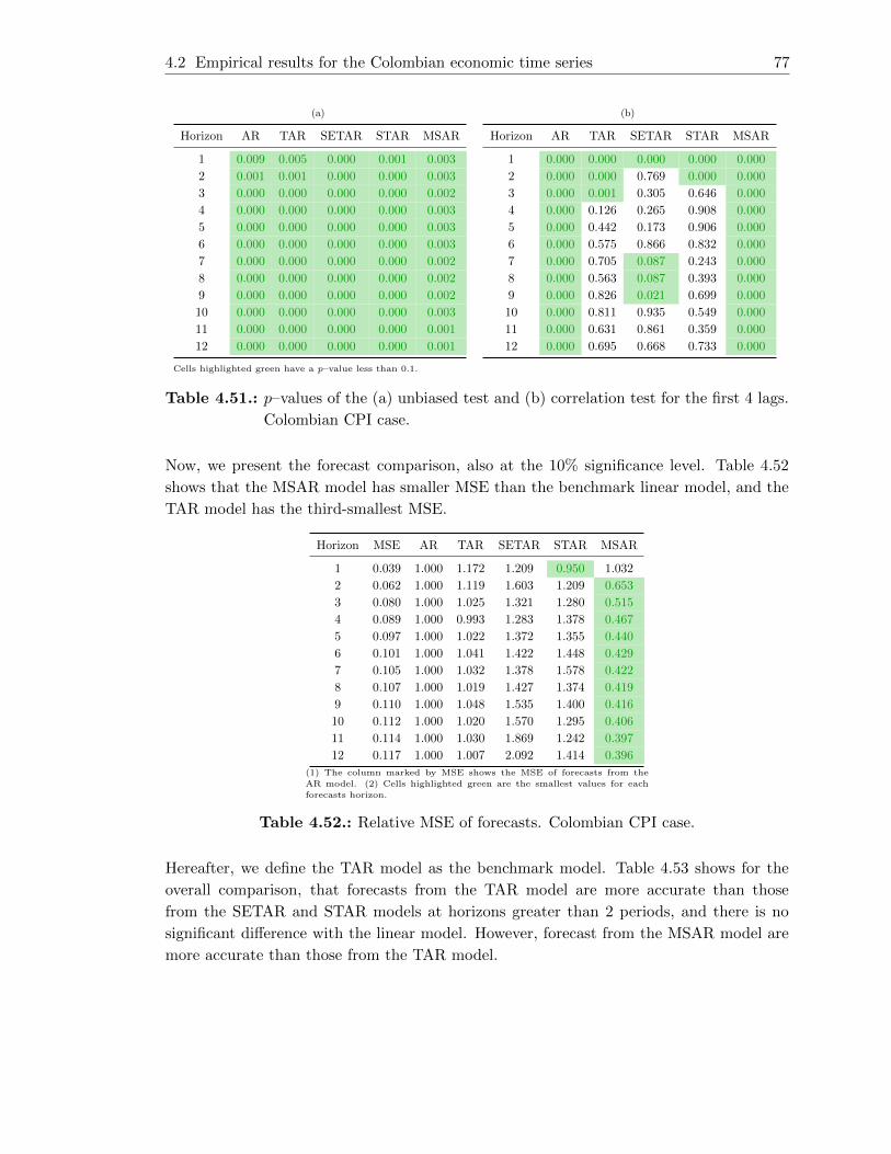
4.2 Empirical results for the Colombian economic time series 77
(a)
Horizon AR TAR SETAR STAR MSAR
1 0.009 0.005 0.000 0.001 0.003
2 0.001 0.001 0.000 0.000 0.003
3 0.000 0.000 0.000 0.000 0.002
4 0.000 0.000 0.000 0.000 0.003
5 0.000 0.000 0.000 0.000 0.003
6 0.000 0.000 0.000 0.000 0.003
7 0.000 0.000 0.000 0.000 0.002
8 0.000 0.000 0.000 0.000 0.002
9 0.000 0.000 0.000 0.000 0.002
10 0.000 0.000 0.000 0.000 0.003
11 0.000 0.000 0.000 0.000 0.001
12 0.000 0.000 0.000 0.000 0.001
(b)
Horizon AR TAR SETAR STAR MSAR
1 0.000 0.000 0.000 0.000 0.000
2 0.000 0.000 0.769 0.000 0.000
3 0.000 0.001 0.305 0.646 0.000
4 0.000 0.126 0.265 0.908 0.000
5 0.000 0.442 0.173 0.906 0.000
6 0.000 0.575 0.866 0.832 0.000
7 0.000 0.705 0.087 0.243 0.000
8 0.000 0.563 0.087 0.393 0.000
9 0.000 0.826 0.021 0.699 0.000
10 0.000 0.811 0.935 0.549 0.000
11 0.000 0.631 0.861 0.359 0.000
12 0.000 0.695 0.668 0.733 0.000
Cells highlighted green have a p–value less than 0.1.
Table 4.51.: p–values of the (a) unbiased test and (b) correlation test for the first 4 lags.
Colombian CPI case.
Now, we present the forecast comparison, also at the 10% significance level. Table 4.52
shows that the MSAR model has smaller MSE than the benchmark linear model, and the
TAR model has the third-smallest MSE.
Horizon MSE AR TAR SETAR STAR MSAR
1 0.039 1.000 1.172 1.209 0.950 1.032
2 0.062 1.000 1.119 1.603 1.209 0.653
3 0.080 1.000 1.025 1.321 1.280 0.515
4 0.089 1.000 0.993 1.283 1.378 0.467
5 0.097 1.000 1.022 1.372 1.355 0.440
6 0.101 1.000 1.041 1.422 1.448 0.429
7 0.105 1.000 1.032 1.378 1.578 0.422
8 0.107 1.000 1.019 1.427 1.374 0.419
9 0.110 1.000 1.048 1.535 1.400 0.416
10 0.112 1.000 1.020 1.570 1.295 0.406
11 0.114 1.000 1.030 1.869 1.242 0.397
12 0.117 1.000 1.007 2.092 1.414 0.396
(1) The column marked by MSE shows the MSE of forecasts from the
AR model. (2) Cells highlighted green are the smallest values for each
forecasts horizon.
Table 4.52.: Relative MSE of forecasts. Colombian CPI case.
Hereafter, we define the TAR model as the benchmark model. Table 4.53 shows for the
overall comparison, that forecasts from the TAR model are more accurate than those
from the SETAR and STAR models at horizons greater than 2 periods, and there is no
significant difference with the linear model. However, forecast from the MSAR model are
more accurate than those from the TAR model.

4.2 Empirical results for the Colombian economic time series 78
(a)
Horizon TAR - AR TAR - SETAR TAR - STAR TAR - MSAR
1 0.016 0.759 0.031 0.016
2 0.057 1.000 0.721 0.001
3 0.324 0.999 0.898 0.000
4 0.560 0.958 0.993 0.000
5 0.185 0.975 0.989 0.000
6 0.121 0.999 0.998 0.000
7 0.111 0.986 1.000 0.000
8 0.234 0.997 0.996 0.000
9 0.069 0.993 1.000 0.000
10 0.229 0.992 0.997 0.000
11 0.109 0.995 0.849 0.000
12 0.382 1.000 0.988 0.000
(b)
Horizon AR - TAR SETAR - TAR STAR - TAR MSAR - TAR
1 0.984 0.241 0.969 0.985
2 0.943 0.000 0.279 0.999
3 0.676 0.001 0.102 1.000
4 0.440 0.042 0.007 1.000
5 0.815 0.025 0.011 1.000
6 0.879 0.001 0.002 1.000
7 0.889 0.014 0.000 1.000
8 0.766 0.003 0.004 1.000
9 0.931 0.007 0.000 1.000
10 0.771 0.008 0.003 1.000
11 0.891 0.005 0.151 1.000
12 0.618 0.000 0.012 1.000
(c)
Horizon TAR - AR TAR - SETAR TAR - STAR TAR - MSAR
1 0.015 0.761 0.030 0.015
2 0.055 1.000 0.723 0.001
3 0.323 0.999 0.900 0.000
4 0.561 0.960 0.993 0.000
5 0.182 0.976 0.980 0.000
6 0.119 0.999 0.998 0.000
7 0.109 0.987 1.000 0.000
8 0.232 0.967 0.992 0.000
9 0.066 0.994 1.000 0.000
10 0.226 0.975 0.992 0.000
11 0.106 0.995 0.780 0.000
12 0.380 1.000 0.948 0.000
(d)
Horizon AR - TAR SETAR - TAR STAR - TAR MSAR - TAR
1 0.985 0.239 0.970 0.985
2 0.945 0.000 0.277 0.999
3 0.677 0.001 0.100 1.000
4 0.439 0.040 0.007 1.000
5 0.818 0.024 0.020 1.000
6 0.881 0.001 0.002 1.000
7 0.891 0.013 0.000 1.000
8 0.768 0.033 0.008 1.000
9 0.934 0.006 0.000 1.000
10 0.774 0.025 0.008 1.000
11 0.894 0.005 0.220 1.000
12 0.620 0.000 0.052 1.000
Cells highlighted green have a p–value less than 0.1.
Table 4.53.: DM test when (a) H1 : Forecasts from competing model (F2) are better than
forecasts from TAR model (F1) and (b) H1 : F1 are better than F2; MDM
test when (c) H1 : F2 are better than F1 and (d) H1 : F1 are better than
F2. Colombian CPI case.
Table 4.54 shows that under the CH test, all the models do not encompass each other.
However, under the ER and HLN tests, the TAR model encompasses the SETAR and
STAR models, but it is encompassed by the linear model at some horizons, in general.
Under the HLN test, the MSAR model could encompass the TAR model.

4.2 Empirical results for the Colombian economic time series 79
(a)
Horizon TAR - AR TAR - SETAR TAR - STAR TAR - MSAR
1 0.001 0.001 0.001 0.000
2 0.000 0.013 0.000 0.000
3 0.000 0.000 0.001 0.000
4 0.000 0.000 0.000 0.000
5 0.000 0.004 0.031 0.000
6 0.000 0.023 0.000 0.000
7 0.000 0.001 0.059 0.000
8 0.000 0.009 0.032 0.000
9 0.000 0.076 0.036 0.000
10 0.000 0.080 0.079 0.000
11 0.000 0.961 0.020 0.000
12 0.000 0.418 0.123 0.000
(b)
Horizon AR - TAR SETAR - TAR STAR - TAR MSAR - TAR
1 0.006 0.000 0.024 0.001
2 0.000 0.000 0.001 0.001
3 0.000 0.000 0.000 0.001
4 0.000 0.000 0.000 0.001
5 0.000 0.000 0.007 0.007
6 0.000 0.000 0.000 0.003
7 0.000 0.000 0.000 0.003
8 0.000 0.002 0.002 0.002
9 0.000 0.000 0.000 0.004
10 0.000 0.001 0.006 0.004
11 0.000 0.000 0.008 0.001
12 0.000 0.000 0.008 0.000
(c)
Horizon TAR - AR TAR - SETAR TAR - STAR TAR - MSAR
1 0.001 0.768 0.000 0.000
2 0.000 0.026 0.337 0.000
3 0.419 0.138 0.922 0.000
4 0.868 0.661 0.384 0.000
5 0.170 0.769 0.437 0.000
6 0.128 0.064 0.174 0.000
7 0.088 0.550 0.010 0.000
8 0.245 0.268 0.225 0.000
9 0.070 0.098 0.078 0.000
10 0.269 0.177 0.307 0.000
11 0.120 0.002 0.821 0.000
12 0.483 0.000 0.159 0.000
(d)
Horizon AR - TAR SETAR - TAR STAR - TAR MSAR - TAR
1 0.076 0.090 0.543 0.029
2 0.020 0.000 0.034 0.021
3 0.915 0.000 0.015 0.029
4 0.637 0.007 0.000 0.012
5 0.684 0.000 0.000 0.001
6 0.405 0.000 0.000 0.006
7 0.433 0.000 0.000 0.007
8 0.782 0.000 0.000 0.008
9 0.245 0.000 0.000 0.005
10 0.736 0.000 0.000 0.007
11 0.431 0.000 0.065 0.005
12 0.906 0.000 0.001 0.007
(e)
Horizon TAR - AR TAR - SETAR TAR - STAR TAR - MSAR
1 0.005 0.385 0.002 0.007
2 0.033 0.991 0.178 0.001
3 0.213 0.932 0.539 0.000
4 0.434 0.676 0.810 0.000
5 0.087 0.615 0.784 0.000
6 0.069 0.956 0.921 0.000
7 0.052 0.727 0.995 0.000
8 0.124 0.871 0.903 0.000
9 0.038 0.929 0.970 0.000
10 0.128 0.899 0.858 0.000
11 0.053 0.979 0.590 0.000
12 0.227 0.999 0.919 0.000
(f)
Horizon AR - TAR SETAR - TAR STAR - TAR MSAR - TAR
1 0.946 0.047 0.725 0.961
2 0.903 0.000 0.018 0.988
3 0.543 0.000 0.009 0.991
4 0.324 0.002 0.000 0.998
5 0.660 0.001 0.000 0.999
6 0.799 0.000 0.000 0.998
7 0.783 0.001 0.000 0.997
8 0.609 0.000 0.000 0.997
9 0.880 0.001 0.000 0.998
10 0.634 0.001 0.000 0.998
11 0.795 0.002 0.036 0.999
12 0.454 0.000 0.001 0.998
Cells highlighted green have a p–value less than 0.1.
Table 4.54.: CH test when (a) H0 : F1 encompasses F2 and (b) H0: F2 encompasses F1;
ER test when (c) H0 : F1 encompasses F2 and (d) H0: F2 encompasses F1;
HLN test when (e) H0 : F1 encompasses F2 and (f) H0: F2 encompasses F1.
Colombian CPI case.
Table 4.55 shows that the MSAR model has the smallest value of the Theil’s U statistic,
followed by the AR and TAR models, and forecasts from the TAR models are more accurate
than those from the SETAR and STAR models.

4.2 Empirical results for the Colombian economic time series 80
Horizon AR TAR SETAR STAR MSAR
1 1.036 1.122 1.140 1.010 1.053
2 1.297 1.373 1.643 1.427 1.048
3 1.454 1.472 1.671 1.645 1.044
4 1.534 1.529 1.738 1.801 1.048
5 1.579 1.597 1.850 1.839 1.047
6 1.598 1.630 1.906 1.923 1.047
7 1.610 1.636 1.890 2.022 1.046
8 1.613 1.628 1.927 1.890 1.044
9 1.624 1.663 2.013 1.922 1.048
10 1.643 1.660 2.059 1.870 1.047
11 1.706 1.731 2.332 1.901 1.074
12 1.708 1.714 2.469 2.030 1.075Cells highlighted green represent the lowest value for each forecast horizon.
Table 4.55.: Theil’s U statistic. Colombian CPI case.
As a summary, it is observed that forecasts errors from all models are not unbiased, and
only the TAR, SETAR and STAR exhibit uncorrelated forecasts errors at horizons greater
than 3 periods. Additionally, Table 4.56 let us observe a satisfactory performance of the
TAR model. According to the Relative MSE of forecasts and the DM and MDM tests, the
TAR model has better MSE of forecasts than the SETAR and STAR models. Regarding
the encompassing tests, the TAR model encompasses the SETAR and STAR models at all
horizons, but it could be compassed by the MSAR model. Additionally, forecasts from all
models are not more accurate than those from the naıve model.
Therefore, from this out-of-sample forecasts comparison, we can conclude that the TAR
model could forecasts the growth rate of the CPI with a reasonable performance, given that
of the alternatives, the TAR model appears to be marginally preferred to the competing
modes.

4.2 Empirical results for the Colombian economic time series 81
Horizon Relative MSE DM - MDM Encompassing tests U-Theil
1 1 0 1 1
(SETAR) (SETAR) (SETAR)
2 2 1 2 2
(SETAR, STAR) (SETAR) (SETAR, STAR) (SETAR, STAR)
3 2 2 2 2
(SETAR, STAR) (SETAR, STAR) (SETAR, STAR) (SETAR, STAR)
4 3 2 2 2
(AR, SETAR, STAR) (SETAR, STAR) (SETAR, STAR) (SETAR, STAR)
5 2 2 2 2
(SETAR, STAR) (SETAR, STAR) (SETAR, STAR) (SETAR, STAR)
6 2 2 2 2
(SETAR, STAR) (SETAR, STAR) (SETAR, STAR) (SETAR, STAR)
7 2 2 2 2
(SETAR, STAR) (SETAR, STAR) (SETAR, STAR) (SETAR, STAR)
8 2 2 2 2
(SETAR, STAR) (SETAR, STAR) (SETAR, STAR) (SETAR, STAR)
9 2 2 2 2
(SETAR, STAR) (SETAR, STAR) (SETAR, STAR) (SETAR, STAR)
10 2 2 2 2
(SETAR, STAR) (SETAR, STAR) (SETAR, STAR) (SETAR, STAR)
11 2 1 2 2
(SETAR, STAR) (SETAR) (SETAR, STAR) (SETAR, STAR)
12 2 2 2 2
(SETAR, STAR) (SETAR, STAR) (SETAR, STAR) (SETAR, STAR)
(1) Cells highlighted green report that the TAR model outperforms 3 or 4 models, highlighted orange report
that the TAR model outperforms 1 or 2 models, and highlighted red report that the TAR model does not
outperform any model. (2) Models in parenthesis are outperformed by the TAR model.
Table 4.56.: Summary of the forecasting performance of the TAR model. Colombian CPI
case.
Finally, we compare the TAR model with the SETAR and STAR models based on their
ability to describe the predictive distribution of the economic time series. As it was men-
tioned before, given that there is not a strong contraction phase during the forecasting
subsample, the 1 to 8-step predictive distributions of the TAR, SETAR and STAR mod-
els tend to be unimodal, capturing the stability of the time series. However, the TAR
model slightly shows bimodal shapes for the lowest values of the CPI, traying to capture
descending periods better than the other models.
As a global summary for the Colombian case, this empirical evaluation shows that forecasts
from the TAR model outperform forecasts from some of the competing models at different
step ahead horizons, for all considered economic times series, although in general, the
forecasting performance of this model is not better than that of the linear model and
the MSAR model. The evaluation criteria let us observe that forecasts from the TAR
model, when using the unemployment rate, outperform those from the competing models
at forecasts horizons greater than 3 periods ahead, and also, it is the model with the best
in-sample properties along with the SETAR model. Regarding the GDP, forecasts from the
TAR model outperform those from the competing models at forecasts horizons between 2
and 7 periods ahead. When using the industrial production index and the CPI time series,

4.2 Empirical results for the Colombian economic time series 82
forecasts from the TAR model only show a better performance than that from the SETAR
and STAR models at all the analyzed forecast horizon, in general. Additionally, given that
the Colombian economic time series do not show a strong contraction phase during the
forecasting period, it was not possible to evaluate the shape changing characteristic in the
Bayesian predictive distributions of the TAR model.

Conclusions
The purpose of this Thesis has been to assess the forecasting performance of the TAR
model. In that sense, we contributed to the literature firstly, by finding the Bayesian
predictive distribution of the TAR model, using the joint predictive distribution that makes
easier the computation of this distributions and reduces the complexity of the definitions of
other approaches; and secondly, by finding important signals about the forecasting ability
of a TAR model in the economic field.
To get those results, we compared the forecasting performance of the TAR model with
that of a linear autoregressive model and nonlinear SETAR, STAR and MSAR models,
using different economic time series of the United States and Colombian economies: the
unemployment rate, the GDP, the industrial production index and the inflation. Therefore,
we estimated 40 models and computed forecasts from all these models.
The results show, globally, good in-sample properties of the TAR model, which means that
the TAR model describes well the characteristics of the economic time series. Additionally,
regarding the forecast evaluation, we found a satisfactory performance of the TAR model
in forecasting all the economic time series, since it outperformed the SETAR and STAR
nonlinear models and the linear model, according to the used evaluation criteria. Regard-
ing the MSAR model, although it has the worst in-sample properties, forecasts from the
MSAR model shows better properties than forecasts from the TAR model. In general,
the TAR model seems marginally preferred to the SETAR, STAR models and AR mod-
els at different forecast horizons, and in some particular cases, to the MSAR model, for
forecasting economic time series, especially, the unemployment rate.
Finally, we found that the Bayesian predictive distributions of the TAR model shows a
shape changing characteristic, with which the TAR model appear to capture business
cycles features of the considered time series better than the other competing models do.
This shape changing quality may suggest that the TAR model can manage cycles in the
economic field and can forecast much better economic time series in contraction periods,
which is important, because it is during this periods that decision and policy makers are
more aware of economic forecasts.
This findings are the base to new fields for research. Some of them are the use of forecasting
combination methods in order to improve forecasts from the TAR model, forecast evalua-
tion during contraction and expansionary periods and reestimating the models throughout
the rolling forecasting procedure, among others.
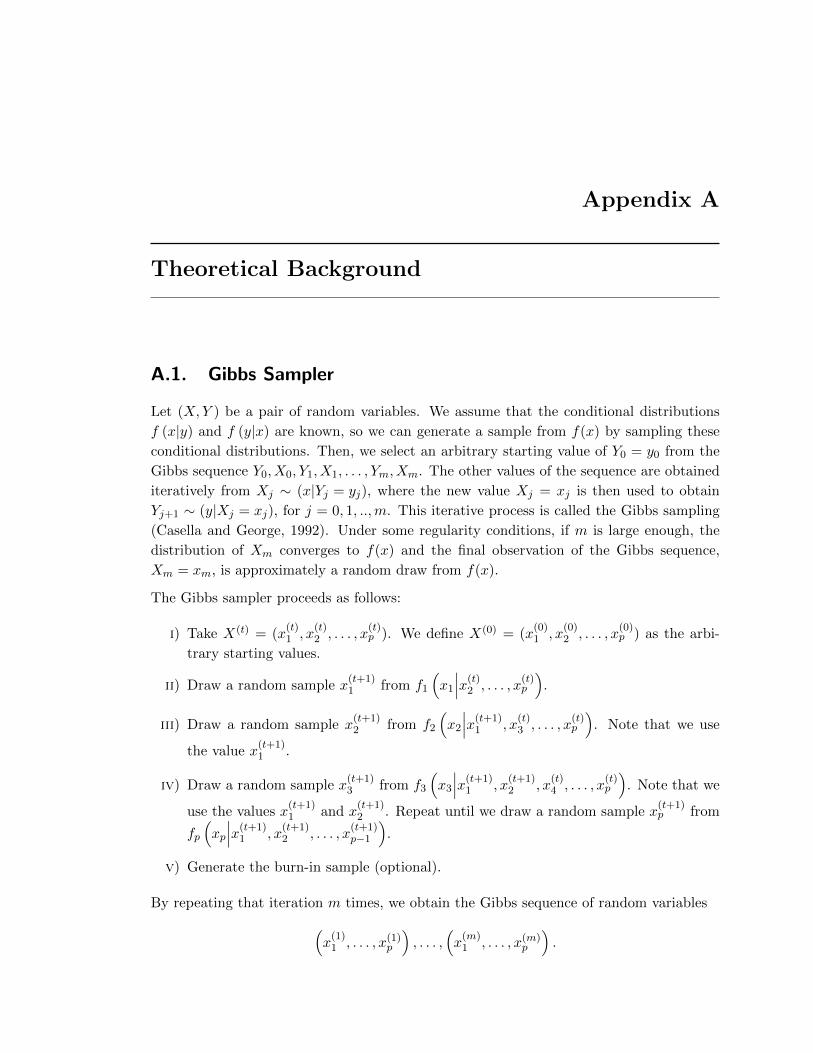
Appendix A
Theoretical Background
A.1. Gibbs Sampler
Let (X,Y ) be a pair of random variables. We assume that the conditional distributions
f (x|y) and f (y|x) are known, so we can generate a sample from f(x) by sampling these
conditional distributions. Then, we select an arbitrary starting value of Y0 = y0 from the
Gibbs sequence Y0, X0, Y1, X1, . . . , Ym, Xm. The other values of the sequence are obtained
iteratively from Xj ∼ (x|Yj = yj), where the new value Xj = xj is then used to obtain
Yj+1 ∼ (y|Xj = xj), for j = 0, 1, ..,m. This iterative process is called the Gibbs sampling
(Casella and George, 1992). Under some regularity conditions, if m is large enough, the
distribution of Xm converges to f(x) and the final observation of the Gibbs sequence,
Xm = xm, is approximately a random draw from f(x).
The Gibbs sampler proceeds as follows:
i) Take X(t) = (x(t)1 , x
(t)2 , . . . , x
(t)p ). We define X(0) = (x
(0)1 , x
(0)2 , . . . , x
(0)p ) as the arbi-
trary starting values.
ii) Draw a random sample x(t+1)1 from f1
(x1
∣∣∣x(t)2 , . . . , x(t)p
).
iii) Draw a random sample x(t+1)2 from f2
(x2
∣∣∣x(t+1)1 , x
(t)3 , . . . , x
(t)p
). Note that we use
the value x(t+1)1 .
iv) Draw a random sample x(t+1)3 from f3
(x3
∣∣∣x(t+1)1 , x
(t+1)2 , x
(t)4 , . . . , x
(t)p
). Note that we
use the values x(t+1)1 and x
(t+1)2 . Repeat until we draw a random sample x
(t+1)p from
fp
(xp
∣∣∣x(t+1)1 , x
(t+1)2 , . . . , x
(t+1)p−1
).
v) Generate the burn-in sample (optional).
By repeating that iteration m times, we obtain the Gibbs sequence of random variables(x(1)1 , . . . , x(1)p
), . . . ,
(x(m)1 , . . . , x(m)
p
).

A.2 Bayesian Predictive Distributions 85
For m large enough,(x(m)1 , . . . , x
(m)p
)is approximately a random draw from the desired dis-
tribution. By using Monte Carlo Integration on those draws, we can obtain the quantities
of interest.
A.2. Bayesian Predictive Distributions
A feature of Bayesian inference are the predictive distributions which allow us to make
inferences about new observations. Let x and θ be the vector of observed data and pa-
rameters respectively, where θ ∈ Θ. For a given model and before the data x is seen, the
distribution of the unknown observable x is defined as (Gelman et al., 2009):
p (x) =
∫Θf (x,θ) dθ =
∫Θf (x|θ) p (θ) dθ. (A.1)
This distribution is called the prior predictive distribution. Once the data x has been
observed, we can predict a new observation x from the model given x:
p (x|x) =
∫Θf (x,θ|x) dθ
=
∫Θf (x|x,θ) f (θ|x) dθ,
(A.2)
which is defined as the posterior predictive distribution (Gelman et al., 2009). Therefore,
that predictive distribution integrates uncertainty about θ and the future value x, both
conditional on x and the assumptions of the proposed model (Geweke and Amisano, 2010).
We note that the predictive distributions do not depend on any unknown quantities but
on the observed data, thus x gives information about θ which gives information about x
(Hoff, 2009).

Appendix B
General review of the models estimation for thechange in the U.S. unemployment rate
B.1. Estimation of the TAR model
We use as the variable of interest the change in the U.S. unemployment rate, that is
Xt = ut − ut−1, where ut is the unemployment rate. As the threshold variable, we use the
growth rate of the U.S. real GDP, that is Zt = [log(GDP t)− log(GDP t−1)] ∗ 100. Figure
B.1 and B.2 show that both series have significant autocorrelations for the first number of
lags.
Figure B.1.: (a) Sample autocorrelation function and (b) sample partial autocorrelation
function for the change in the U.S. unemployment rate.

B.1 Estimation of the TAR model 87
Figure B.2.: (a) Sample autocorrelation function and (b) sample partial autocorrelation
function for the growth rate of U.S. real GDP.
Next, we check the nonlinearity of the series based on Nieto and Hoyos’s (2011) test which
is an extension of Tsay’s (1998) statistic. We test the null hypothesis of AR linearity
against the alternative of bivariate TAR nonlinearity. Under the AIC criterion, we found
that k = 12 is a reasonable autoregressive order for Xt. Under the null hypothesis, the
results of the test let us define the number 0 as the delay parameter of the threshold
variable, thus the input variable for the dynamic system is Zt.
Figure B.3 shows the change in the U.S. quarterly unemployment rate and the growth rate
of the U.S. quarterly real GDP from 1948:02 to 1995:04. The shading areas denote the
business cycle contractions from peak to trough based on NBER.
Figure B.3.: (a) Time plot of the change in the U.S. quarterly unemployment rate and
(b) Time plot of the growth rate of U.S. quarterly real GDP.
We proceed to identify the number of thresholds for the TAR model as indicated in Sec-
tion 1.1. Thus, we specify the maximum number of regimes l0 by means of a regression
function between Xt and Zt that is estimated using a nonparametric kernel approach,
which is presented in Figure B.4. We observe that 3 could be postulated as the possible
maximum regimes for the TAR model, with possible threshold values -1.5 and 1.0 which
could represent periods in the economy of i) contraction, that generates increases in the
unemployment, ii) stabilization, where there is no destruction or creation of employment,

B.1 Estimation of the TAR model 88
and iii) expansion, where there is a decrease in unemployment.
Figure B.4.: Nonparametric regression between the change in the U.S. unemployment
rate (X) and the growth rate of U.S. real GDP (Z).
Once we have defined l0, we select the appropriate thresholds for each possible regimen
l = 2, . . . , l0. That requires to generate intermediate draws of the nonstructural parameters.
Thus, we specify the prior densities for the nonstructural parameters according to Section
1.1. In that sense, we define the prior densities for θx where θ0,j = 0, V −10,j = 0.01I with
I the identity matrix, γ0,j = 1.5 and β0,j = σ2
2 with j = 1, 2, 3 and σ2 = 0.084 that is the
residual variance of the AR(12) that was fitted to the change in the unemployment rate.
The maximum autoregressive order for all regimes is k = 12, the same value fitted to the
change in the unemployment rate. The prior distributions for both the number of regimes
and the autoregressive orders that we use in the identification of l are π2 = π3 = 0.5 and
p (kil|l) = 0.076 for kil = 0, 1, . . . , 12; i = 1, .., l, respectively.
With that information, we identify the thresholds ri; i = 1, . . . , l− 1 for the l0 − 1 possible
models that we denote from now on Mj ; j = 2, . . . , l0 (model M with j regimes). Thus,
to look for the location of thresholds in each possible regime, we choose the percentiles
5k where k = 1, 2, . . . , 19, with respective values -1.00, -0.44, -0.12, 0.19, 0.32, 0.43, 0.56,
0.70, 0.75, 0.85, 0.94, 1.00, 1.13, 1.33, 1.58, 1.74, 1.93, 2.05, 2.42. Then, we choose the
thresholds of the model M2 and M3 by searching among the set of all possible combinations
of autoregressive orders. The possible thresholds and autoregressive orders for each possible
regime are presented in Table B.1.
` Thresholds Autoregressive orders Minimum NAIC
2 0.75 1, 4 1.16734
3 0.19 1.00 11, 1, 4 0.43985
Table B.1.: Set of possible number of regimes for the real data. U.S. unemployment rate
case.
With those possible thresholds and the information mentioned above, we compute the
posterior probability distribution for the number of regimes. 3000 iterates were generated
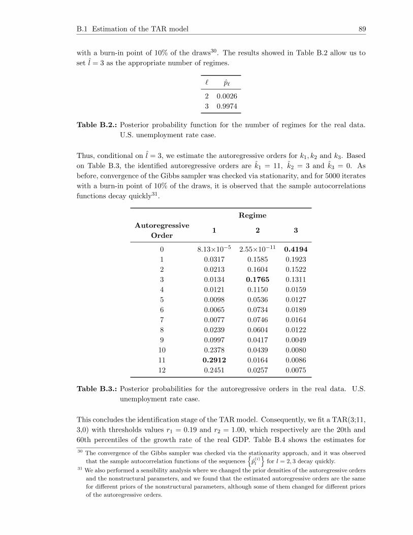
B.1 Estimation of the TAR model 89
with a burn-in point of 10% of the draws30. The results showed in Table B.2 allow us to
set l = 3 as the appropriate number of regimes.
` p`
2 0.0026
3 0.9974
Table B.2.: Posterior probability function for the number of regimes for the real data.
U.S. unemployment rate case.
Thus, conditional on l = 3, we estimate the autoregressive orders for k1, k2 and k3. Based
on Table B.3, the identified autoregressive orders are k1 = 11, k2 = 3 and k3 = 0. As
before, convergence of the Gibbs sampler was checked via stationarity, and for 5000 iterates
with a burn-in point of 10% of the draws, it is observed that the sample autocorrelations
functions decay quickly31.
Regime
Autoregressive
Order1 2 3
0 8.13×10⁻⁵ 2.55×10⁻¹¹ 0.4194
1 0.0317 0.1585 0.1923
2 0.0213 0.1604 0.1522
3 0.0134 0.1765 0.1311
4 0.0121 0.1150 0.0159
5 0.0098 0.0536 0.0127
6 0.0065 0.0734 0.0189
7 0.0077 0.0746 0.0164
8 0.0239 0.0604 0.0122
9 0.0997 0.0417 0.0049
10 0.2378 0.0439 0.0080
11 0.2912 0.0164 0.0086
12 0.2451 0.0257 0.0075
Table B.3.: Posterior probabilities for the autoregressive orders in the real data. U.S.
unemployment rate case.
This concludes the identification stage of the TAR model. Consequently, we fit a TAR(3;11,
3,0) with thresholds values r1 = 0.19 and r2 = 1.00, which respectively are the 20th and
60th percentiles of the growth rate of the real GDP. Table B.4 shows the estimates for
30 The convergence of the Gibbs sampler was checked via the stationarity approach, and it was observed
that the sample autocorrelation functions of the sequences{p(i)l
}for l = 2, 3 decay quickly.
31 We also performed a sensibility analysis where we changed the prior densities of the autoregressive orders
and the nonstructural parameters, and we found that the estimated autoregressive orders are the same
for different priors of the nonstructural parameters, although some of them changed for different priors
of the autoregressive orders.

B.2 Estimation of the SETAR model 90
the nonstructural parameters, with their respective posterior standard error in parenthesis
and 90% credible interval in brackets32. These results show that not all the coefficients are
significant at the 5% significance level. However, we decided to estimate the model with
all the coefficients, given that that improves the final estimation.
Regime
Parameter 1 2 3
a(j)0
0.32 (0.08)
[0.20, 0.45]
0.03 (0.02)
[0.00, 0.07]
-0.25 (0.03)
[−0.30,−0.20]
a(j)1
0.51 (0.21)
[0.17, 0.86]
0.51 (0.07)
[0.40, 0.62]
a(j)2
0.10 (0.31)
[−0.42, 0.61]
-0.04 (0.08)
[−0.18, 0.09]
a(j)3
-0.21 (0.27)
[−0.65, 0.24]
-0.04 (0.07)
[−0.15, 0.08]
a(j)4
-0.24 (0.25)
[−0.64, 0.17]
a(j)5
0.10 (0.31)
[−0.40, 0.61]
a(j)6
0.18 (0.25)
[−0.24, 0.60]
a(j)7
-0.17 (0.28)
[−0.62, 0.30]
a(j)8
-0.95 (0.30)
[−1.46,−0.46]
a(j)9
0.76 (0.31)
[0.26, 1.25]
a(j)10
-0.16 (0.28)
[−0.61, 0.30]
a(j)11
-0.36 (0.24)
[−0.74, 0.02]
h(j)0.12 (0.04)
[0.07, 0.19]
0.03 (0.004)
[0.02, 0.03]
0.07 (0.01)
[0.05, 0.09]
Table B.4.: Parameter estimates for the TAR model. U.S. unemployment rate case.
B.2. Estimation of the SETAR model
To fit a SETAR model for the change in the unemployment rate, as it is mentioned in
Section 1.2, and based on the autocorrelation functions in Figure B.1 and the AIC and
BIC criterion, we determine, in the identification stage, p = 3 as the autoregressive order
32 5000 iterates were generated with a burn-in point of 10% of the draws and it was found that the
autocorrelation functions for all the parameters decay quickly, indicating the convergence of the Gibbs
sampler.

B.3 Estimation of the STAR model 91
but with the second lag restricted to zero.
Once we have selected the autoregressive model, we check the nonlinearity of the series
based on Tsay’s (1989) test and find that with d = 6, where d is the delay parameter, it is
obtained the minimum p-value = 0.029 of the F statistic F = 3.603, rejecting the linearity
of the series at the 5% significance level.
Then, to determine the number of regimes and the threshold values, we use Figure B.5 that
shows the sequence of the t ratios of a lag-3 AR coefficient versus the threshold variable
Xt−6 in an arranged autoregression of order 3, and we identify that the data can be divided
into two regimes with a possible threshold at Xt−d = −0.2, because of the change on the
slope at approximately this point.
Figure B.5.: Time plot of t-ratio of recursive estimates of the AR-3 coefficient in an ar-
ranged autoregression of order 3 and delay parameter 6. U.S. unemployment
rate case.
We also use the NAIC criterion of Tong (1990), which suggests a threshold value of rj =
−0.2 and autoregressive orders AR(1) and AR(3) for each regime, with a NAIC=-439.858.
Therefore, we fit a SETAR(2;1,3) for the change in the US unemployment rate from 1948:2
to 1995:4, with threshold value Xt−6. The estimated parameters and their standard errors
in parenthesis for each regime are shown in Table B.5, where all estimates are significant
at the 5% level.
Regime
Parameter 1 2
Φ(j)1 0.21 (0.09) 0.67 (0.06)
Φ(j)3 -0.21 (0.06)
Table B.5.: Parameter estimates for the SETAR model. U.S. unemployment rate case.
B.3. Estimation of the STAR model
We estimate the STAR model based on Section 1.3. With the identified p = 12 autore-
gressive order, we evaluate the nonlinearity of the series based on Terasvirta’s (1994) test
and find that with the delay parameter d = 1, we obtain the minimum p-value = 0.000 of
the F statistic F = 2.6148, which rejects the linearity of the series.
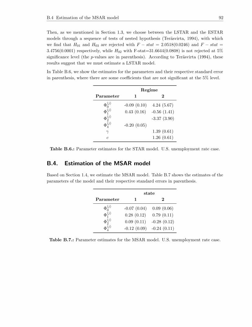
B.4 Estimation of the MSAR model 92
Then, as we mentioned in Section 1.3, we choose between the LSTAR and the ESTAR
models through a sequence of tests of nested hypothesis (Terasvirta, 1994), with which
we find that H01 and H03 are rejected with F − stat = 2.0518(0.0246) and F − stat =
3.4756(0.0001) respectively, while H02 with F-stat=31.6644(0.0808) is not rejected at 5%
significance level (the p-values are in parenthesis). According to Terasvirta (1994), these
results suggest that we must estimate a LSTAR model.
In Table B.6, we show the estimates for the parameters and their respective standard error
in parenthesis, where there are some coefficients that are not significant at the 5% level.
Regime
Parameter 1 2
Φ(j)0 -0.09 (0.10) 4.24 (5.67)
Φ(j)1 0.43 (0.16) -0.56 (1.41)
Φ(j)2 -3.37 (3.90)
Φ(j)4 -0.20 (0.05)
γ 1.39 (0.61)
c 1.26 (0.61)
Table B.6.: Parameter estimates for the STAR model. U.S. unemployment rate case.
B.4. Estimation of the MSAR model
Based on Section 1.4, we estimate the MSAR model. Table B.7 shows the estimates of the
parameters of the model and their respective standard errors in parenthesis.
state
Parameter 1 2
Φ(j)0 -0.07 (0.04) 0.09 (0.06)
Φ(j)1 0.28 (0.12) 0.79 (0.11)
Φ(j)2 0.09 (0.11) -0.28 (0.12)
Φ(j)4 -0.12 (0.09) -0.24 (0.11)
Table B.7.: Parameter estimates for the MSAR model. U.S. unemployment rate case.

Appendix C
General review of the models estimation for theannual growth rate of the U.S. real GDP
C.1. Estimation of the TAR model
We use as the variable of interest the annual growth rate of the U.S. real GDP, and as the
threshold variable, we use the spread term defined in Section 3.2. Figure C.1 and Figure
C.2 show that the autocorrelations are significant for a large number of lags.
Figure C.1.: (a) Sample autocorrelation function and (b) sample partial autocorrelation
function for the annual growth rate of U.S. real GDP.

C.1 Estimation of the TAR model 94
Figure C.2.: (a) Sample autocorrelation function and (b) sample partial autocorrelation
function for the U.S. spread term.
Then, we test the null hypothesis of AR linearity against the alternative of bivariate TAR
nonlinearity. Under the AIC criterion, we found that k = 14 is a reasonable autoregressive
order for Xt. Under the null hypothesis, the results of the test let us define a delay
parameter of 2 for the threshold variable, thus, the input variable for the dynamic system
is Zt−2.
Figure C.3 shows the annual growth rate of the U.S. real GDP and spread term from
1956:01 to 1998:02. The shading areas denote the business cycle contractions from peak
to trough based on NBER.
Figure C.3.: (a) Time plot of the annual growth rate of U.S. real GDP and (b) Time plot
of U.S. spread term.
We specify the maximum number of regimes l0 by means of a regression function between
Xt and Zt, that is estimated using a nonparametric kernel approach and that is presented
in Figure C.4. We observe that 3 could be postulated as the possible maximum regimes
for the TAR model.

C.1 Estimation of the TAR model 95
Figure C.4.: Nonparametric regression between the growth rate of U.S. real GDP (X)
and U.S. spread term (Z).
Next, to specify the prior densities for the nonstructural parameters, we define the prior
densities for θx where θ0,j = 0, V −10,j = 0.01I with I the identity matrix, γ0,j = 1.5 and
β0,j = σ2
2 with j = 1, 2, 3 and σ2 = 0.819 that is the residual variance of the AR(14)
that was fitted to the annual growth of the real GDP. The maximum autoregressive order
for all regimes is k = 14, the same value fitted to the variable of interest. The prior
distributions for both the number of regimes and the autoregressive orders that we use in
the identification of l are π2 = π3 = 0.5 and p (kil|l) = 0.066forkil = 0, 1, . . . , 14; i = 1, .., l,
respectively.
Then, to look for the location of thresholds in each possible regime, we choose the per-
centiles 5k where k = 1, 2, . . . , 19, with respective values -2.90, -1.51, -0.49, -0.16, 0.28,
0.46, 0.59, 0.68, 0.78, 0.96, 1.12, 1.31, 1.52, 1.66, 1.81, 2.09, 2.39, 2.60, 2.91. The possible
thresholds and autoregressive orders for each possible regime are presented in Table C.1.
` Thresholds Autoregressive orders Minimum NAIC
2 0.68 5, 5 3.70792
3 0.59 0.78 11, 13, 12 3.08316
Table C.1.: Set of possible number of regimes for the real data. U.S. GDP case.
With those possible thresholds and the information mentioned above, we compute the
posterior probability distribution for the number of regimes. 3000 iterates were generated
with a burn-in point of 10% of the draws33. The results showed in Table C.2 allow us to
set l = 3 as the appropriate number of regimes.
33 The convergence of the Gibbs sampler was checked via the stationarity approach, where it was observed
that the sample autocorrelation functions of the sequences{p(i)l
}for l = 2, 3 decay quickly.

C.1 Estimation of the TAR model 96
` p`
2 0.41520
3 0.58480
Table C.2.: Posterior probability function for the number of regimes for the real data.
U.S. GDP case.
Thus, conditional on l = 3, we estimate the autoregressive orders for k1, k2 and k3. Based
on Table C.3, the identified autoregressive orders are k1 = 6, k2 = 2 and k3 = 1. As before,
convergence of the Gibbs sampler was checked via stationarity, and for 5000 iterates with a
burn-in point of 10% of the draws, it is observed that the sample autocorrelations functions
decay quickly34.
Regime
Autoregressive
Order1 2 3
0 6.10×10−48 0.0024 1.23×10−49
1 0.0652 0.0468 0.7534
2 0.0243 0.2936 0.2222
3 0.0110 0.1595 0.0195
4 0.0001 0.0520 2.80×10⁻²⁵
5 0.1145 0.0458 0.0001
6 0.2416 0.0237 0.0007
7 0.0979 0.0214 0.0003
8 0.0053 0.0133 9.42×10⁻¹⁸
9 0.0671 0.0928 0.0018
10 0.0874 0.0622 0.0005
11 0.0984 0.0362 0.0009
12 0.0003 0.0300 0.0001
13 0.0945 0.0559 0.0005
Table C.3.: Posterior probabilities for the autoregressive orders in the real data. U.S.
GDP case.
Consequently, we fit a TAR(3;6,2,1) with thresholds values r1 = 0.59 and r2 = 0.78, which
respectively are the 35th and 45th percentiles of the spread term. However, the fitted model
was not appropriate to explain the marginal heteroscedasticity of the data35. Therefore,
34 We also performed a sensibility analysis where we changed the prior densities of the autoregressive orders
and the nonstructural parameters, and we found that the estimated autoregressive orders are the same
for different priors of the nonstructural parameters, although some of them changed for different priors
of the autoregressive orders.35 When we checked the residuals of the estimated TAR(3;6,2,1), we observed that the standardized and
squared standardized residuals of the model slightly signal that some nonlinear structure in the data
is not explained by the model. The Ljung-Box statistics for checking “whiteness” are, respectively,
Q (8) = 19.796(0.011) and Q (8) = 16.365(0.037) with the number in parenthesis denoting the p-value.

C.1 Estimation of the TAR model 97
based on the NAIC criterion36, the estimated model for the change in the annual growth
rate of the U.S. real GDP is a TAR(3;11,13,12) with thresholds values r1 = 0.59 and
r2 = 0.78.
Regime
Parameter 1 2 3
a(j)0
-0.66 (0.60)
[−1.63, 0.35]
-2.95 (3.21)
[−8.14, 2.25]
1.64 (0.26)
[1.22, 2.06]
a(j)1
1.17 (0.16)
[0.90, 1.43]
0.84 (0.54)
[−0.02, 1.73]
0.98 (0.10)
[0.82, 1.14]
a(j)2
-0.08 (0.22)
[−0.43, 0.28]
0.86 (1.87)
[−2.25, 3.93]
-0.05 (0.15)
[−0.29, 0.19]
a(j)3
-0.14 (0.22)
[−0.50, 0.22]
-0.97 (3.94)
[−7.38, 5.50]
-0.18 (0.15)
[−0.44, 0.07]
a(j)4
-0.44 (0.23)
[−0.82,−0.06]
0.71 (2.67)
[−3.67, 5.06]
-0.55 (0.12)
[−0.75,−0.35]
a(j)5
0.47 (0.23)
[0.10, 0.84]
0.04 (0.74)
[−1.12, 1.21]
0.62 (0.14)
[0.40, 0.85]
a(j)6
0.09 (0.24
[−0.29, 0.48]
0.13 (1.48)
[−2.27, 2.49]
-0.01 (0.14)
[−0.25, 0.23]
a(j)7
-0.16 (0.27)
[−0.60, 0.28]
-0.25 (1.86)
[−3.24, 2.85]
-0.03 (0.14)
[−0.27, 0.20]
a(j)8
-0.07 (0.27)
[−0.50, 0.37]
-0.87 (1.83)
[−3.76, 2.08]
-0.42 (0.12)
[−0.62,−0.22]
a(j)9
0.21 (0.24)
[−0.19, 0.61]
1.77 (2.74)
[−2.71, 6.23]
0.36 (0.12)
[0.16, 0.55]
a(j)10
0.05 (0.25)
[−0.36, 0.45]
-0.49 (1.17)
[−2.42, 1.41]
-0.04 (0.13)
[−0.24, 0.17]
a(j)11
-0.09 (0.16)
[−0.36, 0.17]
-0.61 (1.26)
[−2.60, 1.46]
0.07 (0.13)
[−0.14, 0.29]
a(j)12
0.07 (1.23)
[−1.94, 2.09]
-0.14 (0.08)
[−0.27,−0.01]
a(j)13
0.48 (0.57)
[−0.47, 1.43]
h(j)1.32 (0.29)
[0.92, 1.86]
0.40 (0.47)
[0.09, 1.18]
0.53 (0.09)
[0.41, 0.69]
Table C.4.: Parameter estimates for the TAR model. U.S. GDP case.
Table C.4 shows the estimates for the nonstructural parameters, with their respective
The CUSUM and CUSUMSQ indicated that there was no statistical evidence for model misspecification
but there was some heteroscedasticity in {εt}.36 The NAIC criterion for the estimated TAR(3;6,2,1) is 3.718, while for the estimated TAR(3;11,13,12) is
3.022.

C.1 Estimation of the TAR model 98
posterior standard error in parenthesis and 90% credible interval in brackets37. These
results show that not all the coefficients are significant at the 5% level. However, we
decided to estimate the model with all the coefficients, given that that improves the final
estimation.
The fitted TAR model for the change in the annual growth rate of the U.S. real GDP is
given by:
Xt =
−0.66 + 1.17Xt−1 − 0.08Xt−2 − 0.14Xt−3 − 0.44Xt−4
+0.47Xt−5 − 0.09Xt−6 − 0.16Xt−7 − 0.07Xt−8 + 0.21Xt−9
+0.05Xt−10 − 0.09Xt−11 + 1.32εt, if Zt−2 ≤ 0.59
−2.95 + 0.84Xt−1 + 0.86Xt−2 − 0.97Xt−3 + 0.71Xt−4
+0.04Xt−5 + 0.13Xt−6 − 0.25Xt−7 − 0.87Xt−8 + 1.77Xt−9
−0.49Xt−10 − 0.61Xt−11 + 0.07Xt−12 + 0.48Xt−13 + 0.40εt, if 0.59 < Zt−2 ≤ 0.78
1.64 + 0.98Xt−1 − 0.05Xt−2 − 0.18Xt−3 − 0.55Xt−4
+0.62Xt−5 − 0.01Xt−6 − 0.03Xt−7 − 0.42Xt−8 + 0.36Xt−9
−0.04Xt−10 + 0.07Xt−11 − 0.14Xt−12 + 0.53εt, if Zt−2 > 0.78
This model could represent periods in the economy of i) contraction, given that this regime
presents the greatest decreases in the growth rate of the real GDP, when spreads are low
due to contractionary monetary policies; ii) stabilization, where stable spread values are
related to minor variations in the growth rate of the real GDP; and iii) expansion, where
this last regime is associated with the greatest increases in the growth rate of real GDP,
when the monetary policy is expansioning.
When we check the residuals, in Figure C.5 we observe that the standardized and squared
standardized residuals signal that the noise process is white, and the Ljung-Box statistics
for checking “whiteness” are, respectively, Q(8) = 3.805(0.874) and Q(8) = 10.351(0.241).
Figure C.6 reports that the CUSUM and CUSUMSQ behave well, which indicates that
there is no statistical evidence for model misspecification but slightly, some heteroscedas-
ticity in {εt}.
37 5000 iterates were generated with a burn-in point of 10% of the draws, and it was found that the
autocorrelation functions for all the parameters decay quickly, indicating the convergence of the Gibbs
sampler.
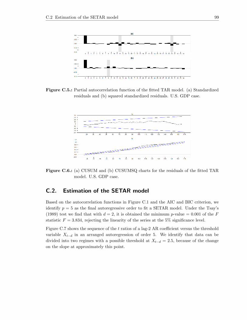
C.2 Estimation of the SETAR model 99
Figure C.5.: Partial autocorrelation function of the fitted TAR model. (a) Standardized
residuals and (b) squared standardized residuals. U.S. GDP case.
Figure C.6.: (a) CUSUM and (b) CUSUMSQ charts for the residuals of the fitted TAR
model. U.S. GDP case.
C.2. Estimation of the SETAR model
Based on the autocorrelation functions in Figure C.1 and the AIC and BIC criterion, we
identify p = 5 as the final autoregressive order to fit a SETAR model. Under the Tsay’s
(1989) test we find that with d = 2, it is obtained the minimum p-value = 0.001 of the F
statistic F = 3.834, rejecting the linearity of the series at the 5% significance level.
Figure C.7 shows the sequence of the t ratios of a lag-2 AR coefficient versus the threshold
variable Xt−d in an arranged autoregression of order 5. We identify that data can be
divided into two regimes with a possible threshold at Xt−d = 2.5, because of the change
on the slope at approximately this point.

C.2 Estimation of the SETAR model 100
Figure C.7.: Time plot of t-ratio of recursive estimates of the AR-2 coefficient in an
arranged autoregression of order 5 and delay parameter 2. U.S. GDP case.
We also use the NAIC criterion of Tong (1990), which suggests a threshold value of rj = 2.29
and autoregressive orders AR(4) and AR(5) for each regime, with a NAIC = 20.769.
Therefore, we fit a SETAR(2;4,5) for the annual growth of the real GDP, with threshold
value Xt−2. The estimated parameters and their standard errors in parenthesis for each
regime are shown in Table C.5 where all estimates are significant at the 5% level, except
the lag-3 AR coefficient of the second regime.
Regime
Parameter 1 2
Φ(j)0 1.60 (0.23)
Φ(j)1 0.86 (0.10) 1.23 (0.08)
Φ(j)2 -0.31 (0.13)
Φ(j)3 0.16 (0.13)
Φ(j)4 -0.55 (-0.55) -0.50 (0.13)
Φ(j)5 0.38 (0.08)
Table C.5.: Parameter estimates for the SETAR model. U.S. GDP case.
In that sense, the estimated SETAR model for the annual growth rate of the U.S. real
GDP, is given by:
Xt =
{1.60 + 0.86Xt−1 − 0.55Xt−4 + εt, if Xt−2 ≤ 2.29
1.23Xt−1 − 0.31Xt−2 + 0.16Xt−3 − 0.50Xt−4 + 0.38Xt−5 + εt, if Xt−2 > 2.29
This model could represent periods in the economy of i) contraction, where the first regime
contains the decreases in the growth rate of the real GDP, that are signaled in the business
cycle contractions of the NBER, and ii) expansion, where the second regime shows the
greatest increases in the growth rate of the real GDP.
Finally, we evaluate the adequacy of the model. Figure C.8 let us observe that the standard-
ized and squared standardized residuals of the model slightly signal that some nonlinear
structure in the data is not explained by the model, and the Ljung-Box statistics are,

C.3 Estimation of the STAR model 101
respectively, Q(8) = 23.636(0.003) and Q(8) = 19.355(0.013). Figure C.9 presents the
CUSUM and CUSUMSQ, which indicate that there is no statistical evidence for model
misspecification but heteroscedasticity in {εt}.
Figure C.8.: Partial autocorrelation function of the fitted SETAR model. (a) Standard-
ized residuals and (b) squared standardized residuals. U.S. GDP case.
Figure C.9.: (a) CUSUM and (b) CUSUMSQ charts for the residuals of the fitted SETAR
model. U.S. GDP case.
C.3. Estimation of the STAR model
With the identified p=12 autoregressive order, we evaluate the nonlinearity of the series
based on Terasvirta’s (1994) test and find that with the delay parameter d = 4, we obtain
the p-value = 0.0074 for the F statistic F = 1.8646, which rejects the linearity of the series.
When we compute the tests of nested hypothesis of Terasvirta (1994), we find that at the
5% significance level, H01 is rejected, while H02 is not, with a respective p - value of 0.0199
and 0.0714. H03 is also not rejected with a p-value = 0.2223. These results suggest that
we must estimate a LSTAR model.
Table C.6 shows the estimates for the parameters and their respective standard error in
parenthesis, which are significant at the 5% level, except for the lag-1 AR coefficient of the
second regime and the parameter γ.

C.3 Estimation of the STAR model 102
Regime
Parameter 1 2
Φ(j)0 0.91 (0.23)
Φ(j)1 1.21 (0.13) -0.18 (0.18)
Φ(j)2 -0.50 (0.18) 0.56 (0.22)
Φ(j)4 -0.54 (0.09)
Φ(j)5 0.25 (0.07)
γ 3.29 (2.27)
c 2.57 (0.61)
Table C.6.: Parameter estimates for the STAR model. U.S. GDP case.
Consequently, the estimated STAR model for the annual growth rate of the U.S. real GDP
is given by:
Xt = 0.91 + 1.21Xt−1 − 0.50Xt−2 − 0.54Xt−4 + 0.25Xt−5
+ F (Xt−4) (−0.18Xt−1 + 0.56Xt−2) + εt,
where
F (Xt−4) = (1 + exp {−3.29 (Xt−4 − 2.57)})−1 .
When we check the residuals, Figure C.10 shows that the standardized and squared stan-
dardized residuals of the estimated model signal that some nonlinear structure in the data
is not explained by the model. Furthermore, the Ljung-Box statistics are, respectively,
Q (8) = 26.906(0.000) and Q (8) = 35.247(0.000). Figure C.11 reports the CUSUM and
CUSUMSQ, which indicate that there is no statistical evidence for model misspecification
but heteroscedasticity in {εt}.
Figure C.10.: Partial autocorrelation function of the fitted STAR model. (a) Standard-
ized residuals and (b) squared standardized residuals. U.S. GDP case.

C.4 Estimation of the MSAR model 103
Figure C.11.: (a) CUSUM and (b) CUSUMSQ charts for the residuals of the fitted STAR
model. U.S. GDP case.
C.4. Estimation of the MSAR model
Table C.7 shows the estimates of the parameters of the model and their respective standard
errors in parenthesis.
state
Parameter 1 2
Φ(j)0 0.42 (0.20) 0.89 (0.29)
Φ(j)1 1.26 (0.10) 1.09 (0.11)
Φ(j)2 -0.14 (0.15) -0.19 (0.16)
Φ(j)3 -0.42 (0.12) -0.24 (0.13)
Φ(j)5 0.18 (0.06) 0.01 (0.08)
Table C.7.: Parameter estimates for the MSAR model. U.S. GDP case.
Therefore, the estimated MSAR model for the annual growth rate of the U.S. real GDP is
given by:
Xt =
{0.42 + 1.26Xt−1 − 0.14Xt−2 − 0.42Xt−4 + 0.18Xt−5 + ε1t, if st = 1
0.89 + 1.09Xt−1 − 0.19Xt−2 − 0.24Xt−4 + 0.01Xt−5 + ε2t, if st = 2
The conditional mean of Xt for regime 1 is -1.59 and for regime 2 is -9.59. The sample
variances of ε1t and ε2t are 0.33 and 2.25, respectively38. Hence, the first state could
represent the stable periods with minor fluctuations in the U.S. economy, and the second
state represents an unstable economy with sharp fluctuations.
Figure C.12 shows that the standardized residuals of the model of the model slightly signal
that some nonlinear structure in the data is not explained by the model. The Ljung-Box
38 The probabilities of moving from one state to the other are p (st = 2|st−1 = 1) = 0.02(0.02) and
p (st = 1|st−1 = 2) = 0.02(0.02), where the number in parenthesis is the standard error. Addition-
ally, the unconditional probability that the process is in regime 1 is 0.52 and that it is in regime 2 is
0.48.

C.5 Estimation of the AR model 104
statistics are, respectively, Q (8) = 92.505(0.000) and Q (8) = 11.006(0.201). Figure C.13
reports the CUSUM and CUSUMSQ, indicating that there is statistical evidence for model
misspecification and heteroscedasticity in {εt}.
Figure C.12.: Partial autocorrelation function of the fitted MSAR model. (a) Standard-
ized residuals and (b) squared standardized residuals. U.S. GDP case.
Figure C.13.: (a) CUSUM and (b) CUSUMSQ charts for the residuals of the fitted MSAR
model. U.S. GDP case.
C.5. Estimation of the AR model
We estimate an AR(5) model for the annual growth rate of the U.S. real GDP39, which is
given by:
(1− 1.15B + 0.23B2 − 0.02B3 + 0.45B4 − 0.30B5
)Xt = 3.35 + at, σ2a = 0.10.
The standard errors of the coefficients are 0.07, 0.11, 0.11, 0.11, 0.07 and 0.39, respectively.
When we check the residuals, Figure C.14 shows that the standardized residuals and the
squared standardized residuals signal that some linear structure in the data is not explained
by the model, and the Ljung-Box statistics are, respectively, Q (8) = 27.477(0.001) and
Q (8) = 37.612(0.000). Figure C.15 shows the CUSUM indicating that there is no statistical
39 As reported by the Augmented Dickey-Fuller (ADF) (p−value = 0.028), Phillips Perron (PP) (p−value =
0.001) and Kwiatkowski-Phillips-Schmidt-Shin (KPSS) (Test statistic = 0.091 and Critical value =
0.463, the growth rate of the U.S. real GDP is stationary at the 5% significance level.

C.5 Estimation of the AR model 105
evidence for model misspecification and CUSUMSQ indicating some statistical evidence
for heteroscedasticity in {εt}.
Figure C.14.: Partial autocorrelation function of the fitted AR model. (a) Standardized
residuals and (b) squared standardized residuals. U.S. GDP case.
Figure C.15.: (a) CUSUM and (b) CUSUMSQ charts for the residuals of the fitted AR
model. U.S. GDP case.
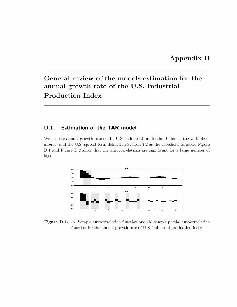
Appendix D
General review of the models estimation for theannual growth rate of the U.S. Industrial
Production Index
D.1. Estimation of the TAR model
We use the annual growth rate of the U.S. industrial production index as the variable of
interest and the U.S. spread term defined in Section 3.2 as the threshold variable. Figure
D.1 and Figure D.2 show that the autocorrelations are significant for a large number of
lags.
Figure D.1.: (a) Sample autocorrelation function and (b) sample partial autocorrelation
function for the annual growth rate of U.S. industrial production index.

D.1 Estimation of the TAR model 107
Figure D.2.: (a) Sample autocorrelation function and (b) sample partial autocorrelation
function for the U.S. spread term.
Then, we test the null hypothesis of AR linearity against the alternative of bivariate TAR
nonlinearity. Under the AIC criterion, we found that k = 13 is a reasonable autoregressive
order for Xt. Under the null hypothesis, the results of the test let us define as the delay
parameter of 2 for the threshold variable, thus, the input variable for the dynamic system
is Zt−2.
Figure D.3 shows the annual growth rate of the U.S. industrial production index and
the spread term from 1960:03 to 1999:04. The shading areas denote the business cycle
contractions from peak to trough based on NBER.
Figure D.3.: (a) Time plot of the annual growth rate of U.S. industrial production index
and (b) Time plot of U.S. spread term.
We specify the maximum number of regimes l0 by means of a regression function between
Xt and Zt, that is estimated using a nonparametric kernel approach that is presented in
Figure D.4. We observe that 3 could be postulated as the possible maximum regimes for
the TAR model.

D.1 Estimation of the TAR model 108
Figure D.4.: Nonparametric regression between the annual growth rate of the U.S. in-
dustrial production index (X) and U.S. spread term (Z).
To specify the prior densities for the nonstructural parameters, we define the prior densities
for θx where θ0,j = 0, V −10,j = 0.01I with I the identity matrix, γ0,j = 1.5 and β0,j = σ2
2
with j = 1, 2, 3 and σ2 = 1.981 that is the residual variance of the AR(13) that was fitted
to the annual growth of the industrial production index. The maximum autoregressive
order for all regimes is k = 13, the same value fitted to the variable of interest. The prior
distributions for both the number of regimes and the autoregressive orders that we use in
the identification of l are π2 = π3 = 0.5 and p (kil|l) = 0.0714 for kil = 0, 1, . . . , 13; i =
1, .., l, respectively.
Then, to look for the location of thresholds in each possible regime, we choose the per-
centiles 5k where k = 1, 2, . . . , 19, with respective values -3.07, -1.60, -0.59, -0.28, -0.05,
0.28, 0.54, 0.67, 0.76, 0.95, 1.12, 1.32, 1.53, 1.68, 1.82, 2.19, 2.40, 2.64, 2.95. The possible
thresholds and autoregressive orders for each possible regime are presented in Table D.1.
` Thresholds Autoregressive orders Minimum NAIC
2 0.76 2, 2 4.57512
3 0.76 1.12 6, 12, 13 3.95755
Table D.1.: Set of possible number of regimes for the real data. U.S. indpro case.
With those possible thresholds and the information mentioned above, we compute the
posterior probability distribution for the number of regimes. 3000 iterates were generated
with a burn-in point of 10% of the draws40. The results showed in Table D.2 allow us to
set l = 3 as the appropriate number of regimes.
40 The convergence of the Gibbs sampler was checked via the stationarity approach, where it was observed
that the sample autocorrelation functions of the sequences{p(i)l
}for l=2,3 decay quickly.
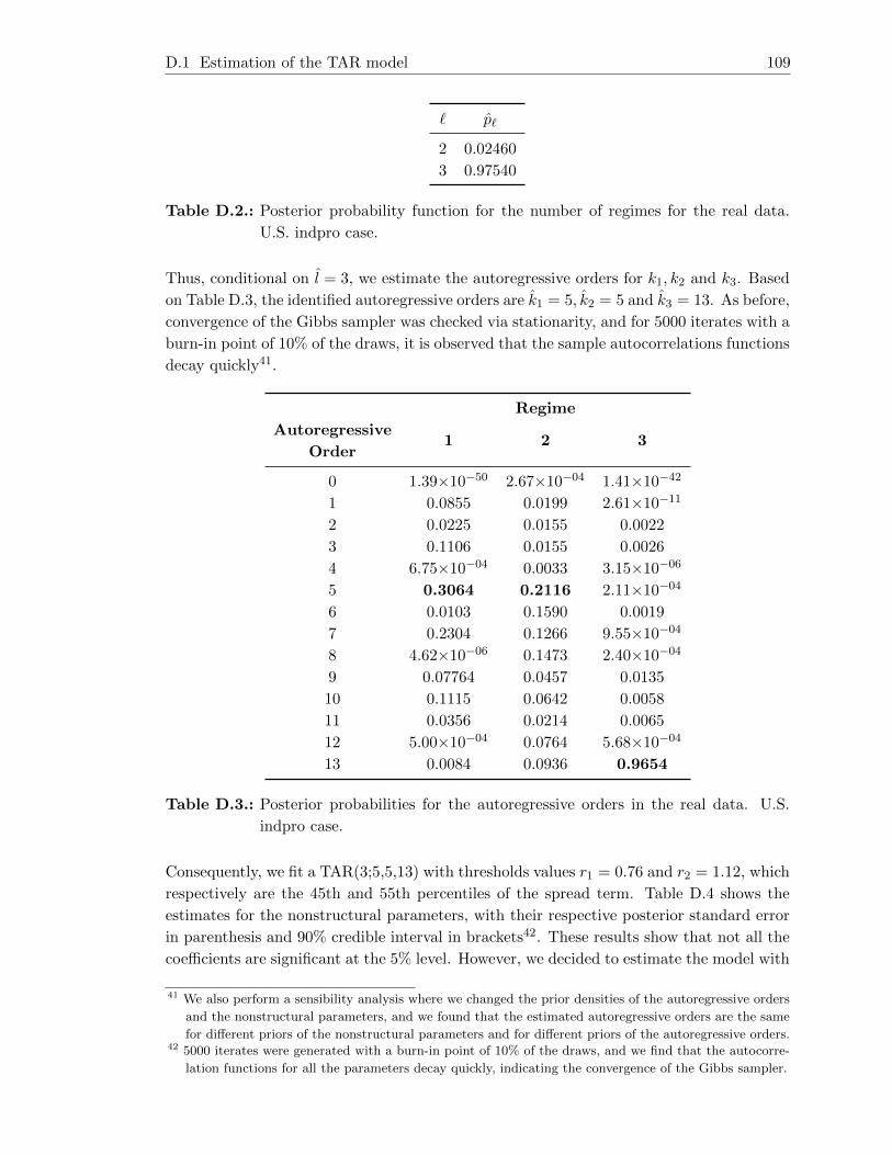
D.1 Estimation of the TAR model 109
` p`
2 0.02460
3 0.97540
Table D.2.: Posterior probability function for the number of regimes for the real data.
U.S. indpro case.
Thus, conditional on l = 3, we estimate the autoregressive orders for k1, k2 and k3. Based
on Table D.3, the identified autoregressive orders are k1 = 5, k2 = 5 and k3 = 13. As before,
convergence of the Gibbs sampler was checked via stationarity, and for 5000 iterates with a
burn-in point of 10% of the draws, it is observed that the sample autocorrelations functions
decay quickly41.
Regime
Autoregressive
Order1 2 3
0 1.39×10−50 2.67×10−04 1.41×10−42
1 0.0855 0.0199 2.61×10⁻¹¹
2 0.0225 0.0155 0.0022
3 0.1106 0.0155 0.0026
4 6.75×10−04 0.0033 3.15×10−06
5 0.3064 0.2116 2.11×10−04
6 0.0103 0.1590 0.0019
7 0.2304 0.1266 9.55×10−04
8 4.62×10−06 0.1473 2.40×10−04
9 0.07764 0.0457 0.0135
10 0.1115 0.0642 0.0058
11 0.0356 0.0214 0.0065
12 5.00×10−04 0.0764 5.68×10−04
13 0.0084 0.0936 0.9654
Table D.3.: Posterior probabilities for the autoregressive orders in the real data. U.S.
indpro case.
Consequently, we fit a TAR(3;5,5,13) with thresholds values r1 = 0.76 and r2 = 1.12, which
respectively are the 45th and 55th percentiles of the spread term. Table D.4 shows the
estimates for the nonstructural parameters, with their respective posterior standard error
in parenthesis and 90% credible interval in brackets42. These results show that not all the
coefficients are significant at the 5% level. However, we decided to estimate the model with
41 We also perform a sensibility analysis where we changed the prior densities of the autoregressive orders
and the nonstructural parameters, and we found that the estimated autoregressive orders are the same
for different priors of the nonstructural parameters and for different priors of the autoregressive orders.42 5000 iterates were generated with a burn-in point of 10% of the draws, and we find that the autocorre-
lation functions for all the parameters decay quickly, indicating the convergence of the Gibbs sampler.

D.1 Estimation of the TAR model 110
all the coefficients, given that that improves the final estimation.
Regime
Parameter 1 2 3
a(j)0
-0.45 (0.40)
[−1.10, 0.21]
0.97 (0.52)
[0.14, 1.80]
1.04 (0.27)
[0.60, 1.48]
a(j)1
1.38 (0.12)
[1.18, 1.59]
1.05 (0.26)
[0.63, 1.47]
1.33 (0.13)
[1.12, 1.53]
a(j)2
-0.57 (0.21)
[−0.92− 0.23]
-0.25 (0.47)
[−1.00, 0.49]
-0.47 (0.20)
[−0.80,−0.15]
a(j)3
0.41 (0.21)
[0.07, 0.75]
0.30 (0.48)
[−0.49, 1.07]
0.09 (0.20)
[−0.24, 0.42]
a(j)4
-0.53 (0.21)
[−0.86,−0.18]
-0.83 (0.43)
[−1.53,−0.13]
-0.70 (0.21)
[−1.05,−0.35]
a(j)5
0.27 (0.14)
[0.03, 0.51]
0.64 (0.27)
[0.20, 1.08]
0.85 (0.23)
[0.46, 1.23]
a(j)6
-0.34 (0.25)
[−0.75, 0.08]
a(j)7
0.19 (0.26)
[−0.23, 0.60]
a(j)8
-0.78 (0.25)
[−1.20,−0.37]
a(j)9
0.88 (0.24)
[0.48, 1.27]
a(j)10
-0.29 (0.22)
[−0.65, 0.06]
a(j)11
0.17 (0.20)
[−0.17, 0.50]
a(j)12
-0.52 (0.17)
[−0.80,−0.24]
a(j)13
0.34 (0.10)
[0.19, 0.50]
h(j)3.21 (0.58)
[2.40, 4.25]
1.27 (0.75)
[0.55, 2.66]
1.02 (0.21)
[0.73, 1.39]
Table D.4.: Parameter estimates for the TAR model. U.S. indpro case.
Therefore, the estimated TAR model for the annual growth rate of the U.S. industrial
production index is given by:

D.1 Estimation of the TAR model 111
Xt =
−0.45 + 1.38Xt−1 − 0.57Xt−2 + 0.41Xt−3 − 0.53Xt−4
+0.27Xt−5 + 3.21εt, if Zt−2 ≤ 0.76
0.97 + 1.05Xt−1 − 0.25Xt−2 + 0.30Xt−3 − 0.83Xt−4
+0.64Xt−5 + 1.27εt, if 0.76 < Zt−2 ≤ 1.12
+0.85Xt−5 − 0.34Xt−6 + 0.19Xt−7 − 0.78Xt−8 + 0.889Xt−9
−0.29Xt−10 + 0.17Xt−11 − 0.52Xt−12 + 0.34Xt−13 + 1.02εt, if Zt−2 > 1.12
This model could represent periods in the economy of i) contraction, given that this regime
contains the greatest decreases in the growth rate of the industrial production index, when
spreads are low due to contractionary monetary policies; ii) stabilization, where stable
spread values are related to minor fluctuations in the growth rate of the industrial produc-
tion index; and iii) expansion, where this last regime exhibits the greatest increases in the
growth rate of the industrial production index, when the monetary policy is expansioning.
When we check the residuals, in Figure D.5 we observe that the standardized residuals
and the squared standardized residuals of the model slightly signal that some nonlinear
structure in the data is not explained by the model. Moreover, the Ljung-Box statistics
are, respectively, Q (8) = 11.554(0.172) and Q (8) = 23.988(0.002). Figure D.6 reports that
the CUSUM and CUSUMSQ behave well, indicating that there is no statistical evidence
for model misspecification but there is some heteroscedasticity in {εt}.
Figure D.5.: Partial autocorrelation function of the fitted TAR model. (a) Standardized
residuals and (b) squared standardized residuals. U.S. indpro case.

D.2 Estimation of the SETAR model 112
Figure D.6.: (a) CUSUM and (b) CUSUMSQ charts for the residuals of the fitted TAR
model. U.S. indpro case.
D.2. Estimation of the SETAR model
Based on the autocorrelation functions in Figure D.1 and the AIC and BIC criterion, we
identify p = 9 as the final autoregressive order to fit a SETAR model. Under the Tsay’s
(1989) test we find that with d = 5, it is obtained the minimum p-value = 0.0004 of the F
statistic F = 3.534, rejecting the linearity of the series at the 5% significance level.
Figure D.7 shows the sequence of the t ratios of a lag-5 AR coefficient versus the threshold
variable Xt−d in an arranged autoregression of order 9, and we identify that the data can
be divided into two regimes with a possible threshold at Xt−d = 5.0, because of the change
on the slope at approximately this point.
Figure D.7.: Time plot of t-ratio of recursive estimates of the AR-5 coefficient in an
arranged autoregression of order 9 and delay parameter 5. U.S. indpro case.
We also use the NAIC criterion of Tong (1990), which suggests a threshold value of rj = 5.08
and autoregressive orders AR(9) and AR(2) for each regime, with a NAIC = 108.918.
Based on that, we fit a SETAR(2;5,2) for the annual growth rate of the industrial produc-
tion index, with threshold value Xt−5. The estimated parameters and their standard errors
in parenthesis for each regime are shown in Table D.5, where all estimates are significant
at the 5% level, although the lag-3 AR coefficient of the first regime is significant at the
10% level.
D.2 Estimation of the SETAR model 113
Regime
Parameter 1 2
Φ(j)0 0.72 (0.20)
Φ(j)1 1.35 (0.10) 1.44 (0.12)
Φ(j)2 -0.59 (0.16) -0.49 (0.11)
Φ(j)3 0.26 (0.15)
Φ(j)4 -0.55 (0.13)
Φ(j)5 0.35 (0.09)
Table D.5.: Parameter estimates for the SETAR model. U.S. indpro case.
Thus, the estimated SETAR model for the annual growth rate of the U.S. industrial pro-
duction index, is given by:
Xt =
0.72 + 1.35Xt−1 − 0.59Xt−2 + 0.26Xt−3
−0.55Xt−4 + 0.35Xt−5 + εt, if Xt−5 ≤ 5.08
1.44Xt−1 − 0.49Xt−2 + εt, if Xt−5 > 5.08
This model could represent periods in the economy of i) contraction, where the first regime
contains mostly the decreases in the growth rate of the industrial production index, and
ii) expansion, where the second regime shows mostly the increases in the growth rate of
the industrial production index.
Figure D.8 let us observe that the standardized and squared standardized residuals of the
model signal that some nonlinear structure in the data is not explained by the model.
Furthermore, the Ljung-Box statistics are, respectively, Q (8) = 28.391(0.000) and Q (8) =
23.980(0.002). Figure D.9 presents the CUSUM and CUSUMSQ, indicating that there is
no statistical evidence for model misspecification but some heteroscedasticity in {εt}.
Figure D.8.: Partial autocorrelation function of the fitted SETAR model. (a) Standard-
ized residuals and (b) squared standardized residuals. U.S. indpro case.

D.3 Estimation of the STAR model 114
Figure D.9.: (a) CUSUM and (b) CUSUMSQ charts for the residuals of the fitted SETAR
model. U.S. indpro case.
D.3. Estimation of the STAR model
With the identified p = 11 autoregressive order, we evaluate the nonlinearity of the series
based on Terasvirta’s (1994) test and find that, with a delay parameter of d = 1, we obtain
the p-value = 0.0067 for the F statistic F = 1.9261, which rejects the linearity of the series.
When we compute the tests of nested hypothesis of Terasvirta (1994), we find that at the
10% significance level, H01 and H03 are rejected, while H02 is not, where the respective
p-value is 0.0605, 0.0116 and 0.2517. These results suggest that we must estimate a LSTAR
model.
In Table D.6, we show the estimates for the parameters and their respective standard error
in parenthesis, which are significant at the 5% significance level, except the parameter γ.
Regime
Parameter 1 2
Φ(j)0 0.46 (0.24)
Φ(j)1 1.79 (0.16) -0.45 (0.18)
Φ(j)2 -1.26 (0.21) 0.67 (0.20)
Φ(j)3 0.33 (0.13)
Φ(j)4 -0.52 (0.12)
Φ(j)5 0.44 (0.11)
Φ(j)6 -0.17 (0.07)
γ 16.55 (44.73)
c -2.93 (1.45)
Table D.6.: Parameter estimates for the STAR model. U.S. indpro case.
Consequently, the estimated STAR model for the annual growth rate of the U.S. industrial
production index is given by:

D.4 Estimation of the MSAR model 115
Xt = 0.46 + 1.79Xt−1 − 1.26Xt−2 + 0.33Xt−3 − 0.52Xt−4 + 0.44Xt−5 − 0.17Xt−6
+ F (Xt−5) (−0.45Xt−1 + 0.67Xt−2) + εt,
where
F (Xt−5) = (1 + exp {−16.55 (Xt−5 + 2.93)})−1 .
When checking the residuals, Figure D.10 shows that the standardized and squared stan-
dardized residuals of the model signal that some nonlinear structure in the data is not
explained by the model. Moreover, the Ljung-Box statistics are, respectively, Q (8) =
21.376(0.006) andQ (8) = 28.559(0.000). Figure D.11 presents the CUSUM and CUSUMSQ,
which indicate that there is no statistical evidence for model misspecification but some het-
eroscedasticity in {εt}.
Figure D.10.: Partial autocorrelation function of the fitted STAR model. (a) Standard-
ized residuals and (b) squared standardized residuals. U.S. indpro case.
Figure D.11.: (a) CUSUM and (b) CUSUMSQ charts for the residuals of the fitted STAR
model. U.S. indpro case.
D.4. Estimation of the MSAR model
Table D.7 shows the estimates of the parameters of the model and their respective standard
errors in parenthesis.

D.4 Estimation of the MSAR model 116
state
Parameter 1 2
Φ(j)0 0.71 (0.18) 0.36 (0.37)
Φ(j)1 1.42 (0.08) 1.32 (0.12)
Φ(j)2 -0.47 (0.10) -0.49 (0.14)
Φ(j)4 -0.33 (0.09) -0.18 (0.15)
Φ(j)5 0.23 (0.07) 0.15 (0.12)
Table D.7.: Parameter estimates for the MSAR model. U.S. indpro case.
Therefore, the estimated MSAR model for the annual growth rate of the U.S. industrial
production index is given by:
Xt =
{0.71 + 1.42Xt−1 − 0.47Xt−2 − 0.33Xt−4 + 0.23Xt−5 + ε1t, if st = 1
0.36 + 1.32Xt−1 − 0.49Xt−2 − 0.18Xt−4 + 0.15Xt−5 + ε2t, if st = 2
The conditional mean of Xt for regime 1 is -1.66 and for regime 2 is -1.11. The sample
variances of ε1t and ε2t are 0.76 and 5.31, respectively43. Hence, the first state could
represent a contractionary economy with reductions in the growth rate of the industrial
production index, and the second state could represent a more stable economy with major
increases in the growth rate of this macroeconomic indicator.
Figure D.12 shows that the standardized and squared standardized residuals of the model
signal that some nonlinear structure in the data is not explained by the model, and the
Ljung-Box statistics are, respectively, Q (8) = 57.790(0.000) and Q (8) = 20.506(0.009).
Figure D.13 presents the CUSUM and CUSUMSQ, which indicate that there is statistical
evidence for model misspecification and some heteroscedasticity in {εt}.
Figure D.12.: Partial autocorrelation function of the fitted MSAR model. (a) Standard-
ized residuals and (b) squared standardized residuals. U.S. indpro case.
43 The probabilities of moving from one state to the other are p (st = 2|st−1 = 1) = 0.05(0.03) and
p (st = 1|st−1 = 2) = 0.06(0.05), where the number in parenthesis is the standard error. Addition-
ally, the unconditional probability that the process is in regime 1 is 0.59 and that it is in regime 2 is
0.41.
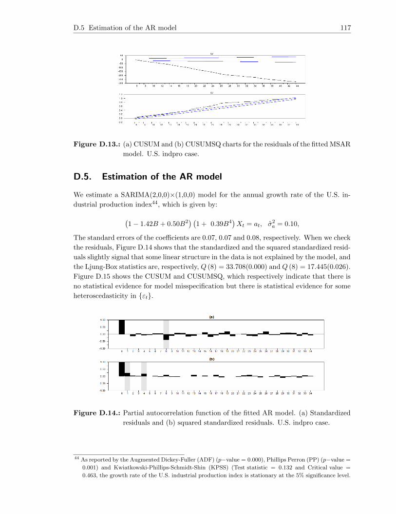
D.5 Estimation of the AR model 117
Figure D.13.: (a) CUSUM and (b) CUSUMSQ charts for the residuals of the fitted MSAR
model. U.S. indpro case.
D.5. Estimation of the AR model
We estimate a SARIMA(2,0,0)×(1,0,0) model for the annual growth rate of the U.S. in-
dustrial production index44, which is given by:
(1− 1.42B + 0.50B2
) (1 + 0.39B4
)Xt = at, σ2a = 0.10,
The standard errors of the coefficients are 0.07, 0.07 and 0.08, respectively. When we check
the residuals, Figure D.14 shows that the standardized and the squared standardized resid-
uals slightly signal that some linear structure in the data is not explained by the model, and
the Ljung-Box statistics are, respectively, Q (8) = 33.708(0.000) and Q (8) = 17.445(0.026).
Figure D.15 shows the CUSUM and CUSUMSQ, which respectively indicate that there is
no statistical evidence for model misspecification but there is statistical evidence for some
heteroscedasticity in {εt}.
Figure D.14.: Partial autocorrelation function of the fitted AR model. (a) Standardized
residuals and (b) squared standardized residuals. U.S. indpro case.
44 As reported by the Augmented Dickey-Fuller (ADF) (p−value = 0.000), Phillips Perron (PP) (p−value =
0.001) and Kwiatkowski-Phillips-Schmidt-Shin (KPSS) (Test statistic = 0.132 and Critical value =
0.463, the growth rate of the U.S. industrial production index is stationary at the 5% significance level.

D.5 Estimation of the AR model 118
Figure D.15.: (a) CUSUM and (b) CUSUMSQ charts for the residuals of the fitted AR
model. U.S. indpro case.

Appendix E
General review of the models estimation for thegrowth rate of the U.S. quarterly CPI
E.1. Estimation of the TAR model
We use as the variable of interest the growth rate of the U.S. CPI, and as the threshold
variable, we use the U.S. spread term mentioned above. Figure E.1 and Figure E.2 show
that the series have significant autocorrelations for a large number of lags.
Figure E.1.: (a) Sample autocorrelation function and (b) sample partial autocorrelation
function for the growth rate of U.S. CPI.
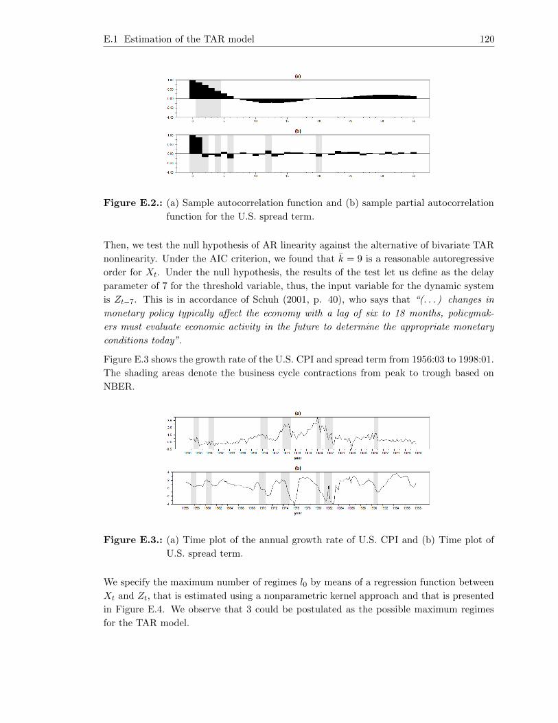
E.1 Estimation of the TAR model 120
Figure E.2.: (a) Sample autocorrelation function and (b) sample partial autocorrelation
function for the U.S. spread term.
Then, we test the null hypothesis of AR linearity against the alternative of bivariate TAR
nonlinearity. Under the AIC criterion, we found that k = 9 is a reasonable autoregressive
order for Xt. Under the null hypothesis, the results of the test let us define as the delay
parameter of 7 for the threshold variable, thus, the input variable for the dynamic system
is Zt−7. This is in accordance of Schuh (2001, p. 40), who says that “(. . . ) changes in
monetary policy typically affect the economy with a lag of six to 18 months, policymak-
ers must evaluate economic activity in the future to determine the appropriate monetary
conditions today”.
Figure E.3 shows the growth rate of the U.S. CPI and spread term from 1956:03 to 1998:01.
The shading areas denote the business cycle contractions from peak to trough based on
NBER.
Figure E.3.: (a) Time plot of the annual growth rate of U.S. CPI and (b) Time plot of
U.S. spread term.
We specify the maximum number of regimes l0 by means of a regression function between
Xt and Zt, that is estimated using a nonparametric kernel approach and that is presented
in Figure E.4. We observe that 3 could be postulated as the possible maximum regimes
for the TAR model.

E.1 Estimation of the TAR model 121
Figure E.4.: Nonparametric regression between the growth rate of U.S. CPI (X) and the
U.S. spread term (Z).
Next, to specify the prior densities for the nonstructural parameters, we define the prior
densities for θx where θ0,j = 0, V −10,j = 0.01I with I the identity matrix, γ0,j = 1.5 and
β0,j = σ2
2 with j = 1, 2, 3 and σ2 = 0.133 that is the residual variance of the AR(9) that was
fitted to the annual growth of the CPI. The maximum autoregressive order for all regimes
is k = 9, the same value fitted to the variable of interest. The prior distributions for both
the number of regimes and the autoregressive orders that we use in the identification of l
are π2 = π3 = 0.5 and p (kil|l) = 0.1 for kil = 0, 1, . . . 9; i = 1, .., l, respectively.
Then, to look for the location of thresholds in each possible regime, we choose the per-
centiles 5k where k = 1, 2, . . . , 19, with respective values -2.95, -1.51, -0.50, -0.18, 0.23,
0.46, 0.59, 0.68, 0.81, 0.96, 1.18, 1.32, 1.57, 1.67, 1.82, 2.10, 2.39, 2.61, 2.92. The possible
thresholds and autoregressive orders for each possible regime are presented in Table E.1.
` Thresholds Autoregressive orders Minimum NAIC
2 0.68 3, 3 1.62567
3 -0.18 1.18 3, 2, 3 1.16958
Table E.1.: Set of possible number of regimes for the real data. U.S. CPI case.
With those possible thresholds and the information mentioned above, we compute the
posterior probability distribution for the number of regimes. 3000 iterates were generated
with a burn-in point of 10% of the draws45. The results showed in Table E.2 allow us to
set l = 3 as the appropriate number of regimes.
` p`
2 0.3068
3 0.6932
Table E.2.: Posterior probability function for the number of regimes for the real data.
U.S. CPI case.
45 The convergence of the Gibbs sampler was checked via the stationarity approach, where it was observed
that the sample autocorrelation functions of the sequences{p(i)l
}for l = 2, 3 decay quickly.
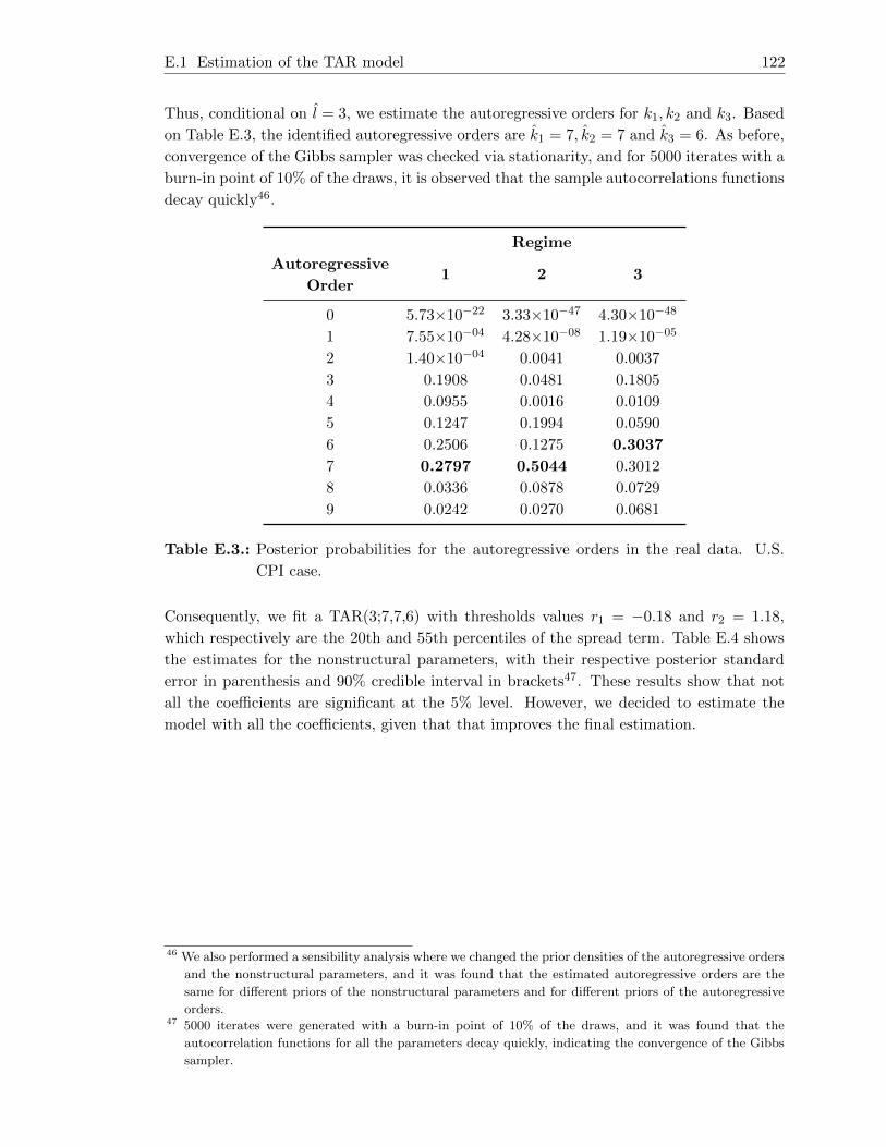
E.1 Estimation of the TAR model 122
Thus, conditional on l = 3, we estimate the autoregressive orders for k1, k2 and k3. Based
on Table E.3, the identified autoregressive orders are k1 = 7, k2 = 7 and k3 = 6. As before,
convergence of the Gibbs sampler was checked via stationarity, and for 5000 iterates with a
burn-in point of 10% of the draws, it is observed that the sample autocorrelations functions
decay quickly46.
Regime
Autoregressive
Order1 2 3
0 5.73×10⁻²² 3.33×10−47 4.30×10−48
1 7.55×10−04 4.28×10−08 1.19×10−05
2 1.40×10−04 0.0041 0.0037
3 0.1908 0.0481 0.1805
4 0.0955 0.0016 0.0109
5 0.1247 0.1994 0.0590
6 0.2506 0.1275 0.3037
7 0.2797 0.5044 0.3012
8 0.0336 0.0878 0.0729
9 0.0242 0.0270 0.0681
Table E.3.: Posterior probabilities for the autoregressive orders in the real data. U.S.
CPI case.
Consequently, we fit a TAR(3;7,7,6) with thresholds values r1 = −0.18 and r2 = 1.18,
which respectively are the 20th and 55th percentiles of the spread term. Table E.4 shows
the estimates for the nonstructural parameters, with their respective posterior standard
error in parenthesis and 90% credible interval in brackets47. These results show that not
all the coefficients are significant at the 5% level. However, we decided to estimate the
model with all the coefficients, given that that improves the final estimation.
46 We also performed a sensibility analysis where we changed the prior densities of the autoregressive orders
and the nonstructural parameters, and it was found that the estimated autoregressive orders are the
same for different priors of the nonstructural parameters and for different priors of the autoregressive
orders.47 5000 iterates were generated with a burn-in point of 10% of the draws, and it was found that the
autocorrelation functions for all the parameters decay quickly, indicating the convergence of the Gibbs
sampler.
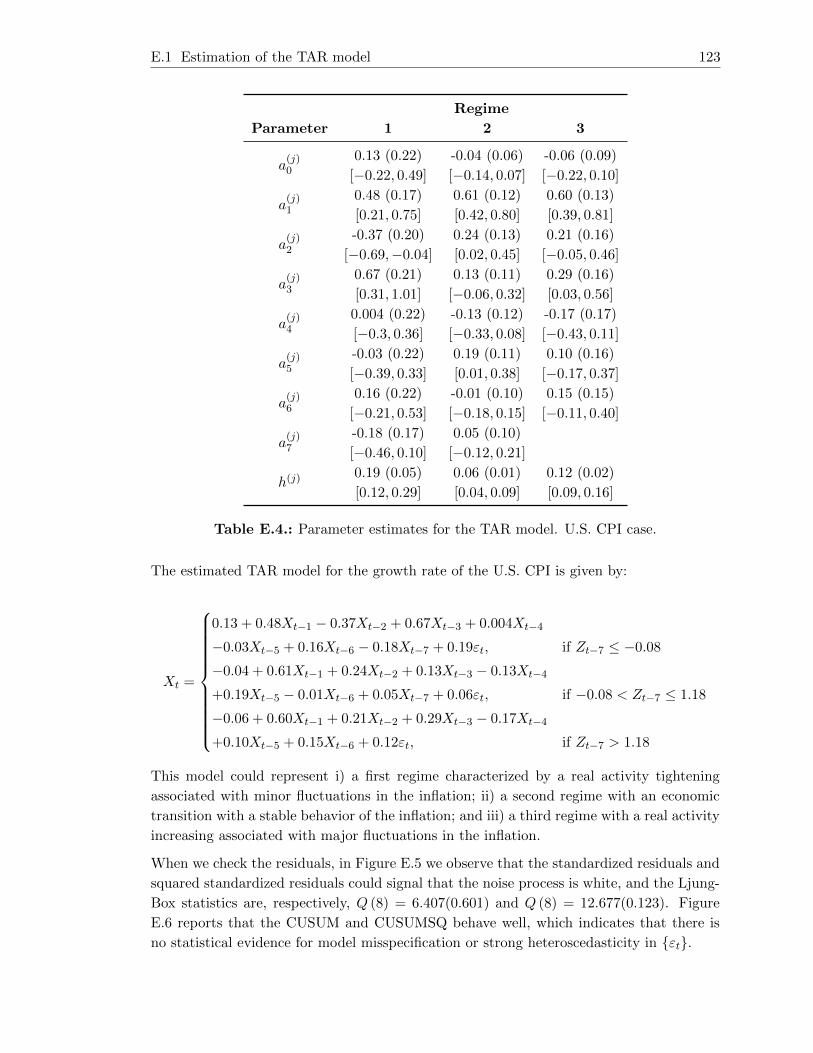
E.1 Estimation of the TAR model 123
Regime
Parameter 1 2 3
a(j)0
0.13 (0.22)
[−0.22, 0.49]
-0.04 (0.06)
[−0.14, 0.07]
-0.06 (0.09)
[−0.22, 0.10]
a(j)1
0.48 (0.17)
[0.21, 0.75]
0.61 (0.12)
[0.42, 0.80]
0.60 (0.13)
[0.39, 0.81]
a(j)2
-0.37 (0.20)
[−0.69,−0.04]
0.24 (0.13)
[0.02, 0.45]
0.21 (0.16)
[−0.05, 0.46]
a(j)3
0.67 (0.21)
[0.31, 1.01]
0.13 (0.11)
[−0.06, 0.32]
0.29 (0.16)
[0.03, 0.56]
a(j)4
0.004 (0.22)
[−0.3, 0.36]
-0.13 (0.12)
[−0.33, 0.08]
-0.17 (0.17)
[−0.43, 0.11]
a(j)5
-0.03 (0.22)
[−0.39, 0.33]
0.19 (0.11)
[0.01, 0.38]
0.10 (0.16)
[−0.17, 0.37]
a(j)6
0.16 (0.22)
[−0.21, 0.53]
-0.01 (0.10)
[−0.18, 0.15]
0.15 (0.15)
[−0.11, 0.40]
a(j)7
-0.18 (0.17)
[−0.46, 0.10]
0.05 (0.10)
[−0.12, 0.21]
h(j)0.19 (0.05)
[0.12, 0.29]
0.06 (0.01)
[0.04, 0.09]
0.12 (0.02)
[0.09, 0.16]
Table E.4.: Parameter estimates for the TAR model. U.S. CPI case.
The estimated TAR model for the growth rate of the U.S. CPI is given by:
Xt =
0.13 + 0.48Xt−1 − 0.37Xt−2 + 0.67Xt−3 + 0.004Xt−4
−0.03Xt−5 + 0.16Xt−6 − 0.18Xt−7 + 0.19εt, if Zt−7 ≤ −0.08
−0.04 + 0.61Xt−1 + 0.24Xt−2 + 0.13Xt−3 − 0.13Xt−4
+0.19Xt−5 − 0.01Xt−6 + 0.05Xt−7 + 0.06εt, if −0.08 < Zt−7 ≤ 1.18
−0.06 + 0.60Xt−1 + 0.21Xt−2 + 0.29Xt−3 − 0.17Xt−4
+0.10Xt−5 + 0.15Xt−6 + 0.12εt, if Zt−7 > 1.18
This model could represent i) a first regime characterized by a real activity tightening
associated with minor fluctuations in the inflation; ii) a second regime with an economic
transition with a stable behavior of the inflation; and iii) a third regime with a real activity
increasing associated with major fluctuations in the inflation.
When we check the residuals, in Figure E.5 we observe that the standardized residuals and
squared standardized residuals could signal that the noise process is white, and the Ljung-
Box statistics are, respectively, Q (8) = 6.407(0.601) and Q (8) = 12.677(0.123). Figure
E.6 reports that the CUSUM and CUSUMSQ behave well, which indicates that there is
no statistical evidence for model misspecification or strong heteroscedasticity in {εt}.

E.2 Estimation of the SETAR model 124
Figure E.5.: Partial autocorrelation function of the fitted TAR model. (a) Standardized
residuals and (b) squared standardized residuals. U.S. CPI case.
Figure E.6.: (a) CUSUM and (b) CUSUMSQ charts for the residuals of the fitted TAR
model. U.S. CPI case.
E.2. Estimation of the SETAR model
Based on the autocorrelation functions in Figure E.1 and the AIC and BIC criterion, we
identify p = 9 as the final autoregressive order to fit a SETAR model. Under the Tsay’s
(1989) test and we find that with d = 2, it is obtained the minimum p-value = 0.0035 of
the F statistic F = 2.795, rejecting the linearity of the series at the 5% significance level.
Figure E.7 shows the sequence of the t ratios of a lag-9 AR coefficient versus the threshold
variable Xt−d in an arranged autoregression of order 9. We identify that data can be
divided into two regimes with a possible threshold at Xt−d = 1.0, because of the change
on the slope at approximately this point.

E.2 Estimation of the SETAR model 125
Figure E.7.: Time plot of t-ratio of recursive estimates of the AR-9 coefficient in an
arranged autoregression of order 9 and delay parameter 2. U.S. CPI case.
We also use the NAIC criterion of Tong (1990), which suggests a threshold value of rj = 0.98
and autoregressive orders AR(3) and AR(4) for each regime, with a NAIC = -345.436.
Based on that, we fit a SETAR(2;3,4) for the growth rate of the CPI, with threshold value
Xt−2. The estimated parameters and their standard errors in parenthesis for each regime
are shown in Table E.5 where all estimates are significant at the 5% level, except the
constant coefficient of both regimes.
Regime
Parameter 1 2
Φ(j)0 0.10 (0.07) -0.02 (0.14)
Φ(j)1 0.45 (0.09) 0.83 (0.10)
Φ(j)2 0.20 (0.12)
Φ(j)3 0.28 (0.08) 0.65 (0.13)
Φ(j)4 -0.53 (0.14)
Table E.5.: Parameter estimates for the SETAR model. U.S. CPI case.
Thus, the estimated SETAR model for the growth rate of the U.S. CPI, is given by:
Xt =
{0.10 + 0.45Xt−1 + 0.20Xt−2 + 0.28Xt−3 + εt, if Xt−2 ≤ 0.98
−0.02 + 0.83Xt−1 + 0.65Xt−3 − 0.53Xt−4 + εt, if Xt−2 > 0.98
This model could represent i) a first regime characterized by a real activity tightening
associated with minor fluctuations in the inflation; and ii) a second regime with a real
activity increasing associated with major fluctuations in the inflation.
Figure E.8 shows that the standardized and squared standardized residuals of the model
could signal that the noise process is white. Furthermore, the Ljung-Box statistics are,
respectively, Q (8) = 11.517(0.174) and Q (8) = 7.190(0.516). Figure E.9 presents the
CUSUM and CUSUMSQ, which indicate that there is no statistical evidence for model
misspecification or strong heteroscedasticity in {εt}.
E.3 Estimation of the STAR model 126
Figure E.8.: Partial autocorrelation function of the fitted SETAR model. (a) Standard-
ized residuals and (b) squared standardized residuals. U.S. CPI case.
Figure E.9.: (a) CUSUM and (b) CUSUMSQ charts for the residuals of the fitted SETAR
model. U.S. CPI case.
E.3. Estimation of the STAR model
With the identified p = 11 autoregressive order, we evaluate the nonlinearity of the series
based on Terasvirta’s (1994) test and find that, with a delay parameter of d = 1, we obtain
the p-value = 0.0011 for the F statistic F = 2.2235, which rejects the linearity of the series.
When we compute the tests of nested hypothesis of Terasvirta (1994), we find that at the
10% significance level, H01 and H03 are rejected, while H02 is not, where the respective p-
value are 0.0870, 0.0016 and 0.1056. These results suggest that we must estimate a LSTAR
model.
In Table E.6 we show the estimates for the parameters and their respective standard error
in parenthesis, where only the lag-3 and lag-4 AR coefficient of the first regime and the
parameter γ are significant at the 5% level.

E.3 Estimation of the STAR model 127
Regime
Parameter 1 2
Φ(j)0 0.70 (0.80)
Φ(j)1 -0.60 (1.09) 1.13 (1.27)
Φ(j)3 0.41 (0.08)
Φ(j)4 -0.22 (0.08)
γ 1.29 (0.35)
c 0.32 (1.07)
Table E.6.: Parameter estimates for the STAR model. U.S. CPI case.
Consequently, the estimated STAR model for the growth rate of the U.S. CPI is given by:
Xt = −0.60Xt−1 + 0.41Xt−3 − 0.22Xt−4 + F (Xt−1) (070 + 1.13Xt−1) + εt,
where
F (Xt−1) = (1 + exp {−1.29 (Xt−1 − 0.32)})−1 .
When we check the residuals, Figure E.10 shows that the standardized and squared stan-
dardized residuals signal that some nonlinear structure in the data is not explained by the
model. Additionally, the Ljung-Box statistics are, respectively, Q (8) = 13.957(0.083) and
Q (8) = 17.068(0.029). Figure E.11 presents the CUSUM and CUSUMSQ, which indicate
that there is no statistical evidence for model misspecification but some heteroscedasticity
in {εt}.
Figure E.10.: Partial autocorrelation function of the fitted STAR model. (a) Standard-
ized residuals and (b) squared standardized residuals. U.S. CPI case.
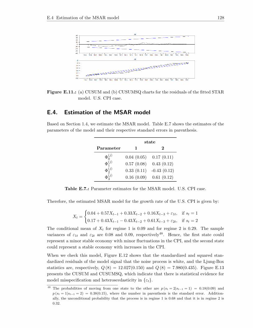
E.4 Estimation of the MSAR model 128
Figure E.11.: (a) CUSUM and (b) CUSUMSQ charts for the residuals of the fitted STAR
model. U.S. CPI case.
E.4. Estimation of the MSAR model
Based on Section 1.4, we estimate the MSAR model. Table E.7 shows the estimates of the
parameters of the model and their respective standard errors in parenthesis.
state
Parameter 1 2
Φ(j)0 0.04 (0.05) 0.17 (0.11)
Φ(j)1 0.57 (0.08) 0.43 (0.12)
Φ(j)2 0.33 (0.11) -0.43 (0.12)
Φ(j)3 0.16 (0.09) 0.61 (0.12)
Table E.7.: Parameter estimates for the MSAR model. U.S. CPI case.
Therefore, the estimated MSAR model for the growth rate of the U.S. CPI is given by:
Xt =
{0.04 + 0.57Xt−1 + 0.33Xt−2 + 0.16Xt−3 + ε1t, if st = 1
0.17 + 0.43Xt−1 − 0.43Xt−2 + 0.61Xt−3 + ε2t, if st = 2
The conditional mean of Xt for regime 1 is 0.09 and for regime 2 is 0.29. The sample
variances of ε1t and ε2t are 0.08 and 0.09, respectively48. Hence, the first state could
represent a minor stable economy with minor fluctuations in the CPI, and the second state
could represent a stable economy with increases in the CPI.
When we check this model, Figure E.12 shows that the standardized and squared stan-
dardized residuals of the model signal that the noise process is white, and the Ljung-Box
statistics are, respectively, Q (8) = 12.027(0.150) and Q (8) = 7.980(0.435). Figure E.13
presents the CUSUM and CUSUMSQ, which indicate that there is statistical evidence for
model misspecification and heteroscedasticity in {εt}.48 The probabilities of moving from one state to the other are p (st = 2|st−1 = 1) = 0.18(0.09) and
p (st = 1|st−1 = 2) = 0.38(0.15), where the number in parenthesis is the standard error. Addition-
ally, the unconditional probability that the process is in regime 1 is 0.68 and that it is in regime 2 is
0.32.

E.5 Estimation of the AR model 129
Figure E.12.: Partial autocorrelation function of the fitted MSAR model. (a) Standard-
ized residuals and (b) squared standardized residuals. U.S. CPI case.
Figure E.13.: (a) CUSUM and (b) CUSUMSQ charts for the residuals of the fitted MSAR
model. U.S. CPI case.
E.5. Estimation of the AR model
We estimate an AR(4) model for the growth rate of the U.S. CPI49, which is given by:
(1− 0.70B + 0.06B2 − 0.46B3 + 0.21B4
)Xt = 1.03 + at, σ2a = 0.14,
The standard errors of the coefficients are 0.08, 0.09, 0.09, 0.09 and 0.26, respectively.
When we check the residuals, Figure E.14 shows that the standardized and the squared
standardized residuals slightly signal that some linear structure in the data is not explained
by the model, and the Ljung-Box statistics are, respectively, Q (8) = 10.004(0.265) and
Q (8) = 17.396(0.026). Figure E.15 shows the CUSUM and CUSUMSQ, which respec-
tively indicate that there is no statistical evidence for model misspecification, but there is
statistical evidence for some heteroscedasticity in εt.
49 As reported by the Augmented Dickey-Fuller (ADF) (p−value = 0.089), Phillips Perron (PP) (p−value =
0.005) and Kwiatkowski-Phillips-Schmidt-Shin (KPSS) (Test statistic = 0.374 and Critical value =
0.463, the growth rate of the growth rate of the U.S. CPI is stationary at the 5% significance level.

E.5 Estimation of the AR model 130
Figure E.14.: Partial autocorrelation function of the fitted AR model. (a) Standardized
residuals and (b) squared standardized residuals. U.S. CPI case.
Figure E.15.: (a) CUSUM and (b) CUSUMSQ charts for the residuals of the fitted AR
model. U.S. CPI case.

Appendix F
General review of the model estimation for thechange in the Colombian unemployment rate
F.1. Estimation of the TAR model
We use as the variable of interest the change in the Colombian unemployment rate, that
is Xt = ut − ut−1, where ut is the unemployment rate. As the threshold variable, we use
the growth rate of the ISE index, that is Zt = [log(ISEt)− log(ISEt−1)] ∗ 100.
Figure F.1 shows that the series have significant autocorrelations at the first two lags.
Figure F.2 shows that series have significant autocorrelations at lags 1, 4, 9 and 10.
Figure F.1.: (a) Autocorrelation function and (b) partial autocorrelation function for
change in the Colombian unemployment rate.

F.1 Estimation of the TAR model 132
Figure F.2.: (a) Autocorrelation function and (b) partial autocorrelation function for the
growth rate of Colombian ISE index.
After that, we test the null hypothesis of AR process linearity against the alternative
of bivariate TAR nonlinearity. We apply the statistic to different lags of the threshold
variable, that is, Zt−d, d = 1, . . . , 10. Under the AIC criterion, we found that k = 3 is a
reasonable autoregressive order for Xt. The results of the test let us define d = 2 as the
delay parameter of the threshold variable, consequently the input variable for the dynamic
system is Zt−2.
Figure F.3 shows the change in the Colombian unemployment rate and in the growth rate
of the ISE index, where the latter is lagged 2 months. We can observe in some periods
the countercyclical behavior between both series, that is, fallings in the ISE index with
raisings in the unemployment rate.
Figure F.3.: Growth rate of Colombian ISE index lagged 2 months and change in the
Colombian unemployment rate.
The next step is identifying the number of thresholds for the TAR model as indicated in
Section 1.1. Thus, we specify the maximum number of regimes l0 by means of a regression
function between Xt and Zt, that is estimated using a nonparametric kernel approach
and that is presented in Figure F.4. We observe that 3 could be postulated as the possible
maximum regimes for the TAR model, with possible threshold values -0.90 and 0.10. Those
possible regimes could represent periods in the economy of i) contraction that generates
increases of unemployment, ii) stabilization where there is no destruction or creation of
employment, and iii) expansion where there is a decrease of unemployment.

F.1 Estimation of the TAR model 133
Figure F.4.: Nonparametric regression between the change in the Colombian unemploy-
ment rate (X) and the growth rate of Colombian ISE index (Z).
Once we have defined l0, we select the appropriate thresholds for each possible regimen l =
2, . . . , l0, which requires to generate intermediate draws of the nonstructural parameters.
Thus, we specify the prior densities for the nonstructural parameters as stated in Section
1.1. In that sense, we define the prior densities for θx, with θ0,j = 0, V −10,j = 0.01I where
I is the identity matrix, γ0,j = 1.5 and β0,j = σ2
2 with j = 1, 2, 3 and σ2 = 0.31 is
the residual variance of the AR(3) fitted to the change in the Colombian unemployment
rate. The maximum autoregressive order for all regimes is k = 3, the same order fitted
to the change in the Colombian unemployment rate. The prior distributions for both the
number of regimes and the autoregressive orders that we use in the identification of l are
π2 = π3 = 0.5 and p (kil|l) = 0.25 for kil = 0, 1, 2, 3, and i = 1, . . . , l.
With that information, we identify the thresholds ri; i = 1, . . . , l− 1 for the l0 − 1 possible
M models with j regimes, denoted Mj ; j = 2, . . . , l0. Then, to look for the location of
thresholds in each possible regime, we choose the percentiles 5k where k = 1, 2, . . . , 19,
with respective values -0.83, -0.44, -0.33, -0.13, -0.02, 0.10, 0.15, 0.24, 0.32, 0.36, 0.45,
0.50, 0.54, 0.70, 0.89, 0.94, 1.05, 1.15, 1.47. Then, we choose the threshold of model M2
and M3 by searching among the set of all possible combinations of autoregressive orders.
The possible thresholds and autoregressive orders for each possible regime are presented
in Table F.1.
` Thresholds Autoregressive orders Minimum NAIC
2 0.32 2, 1 2.37152
3 0.15 0.54 2, 1, 2 1.95958
Table F.1.: Set of possible number of regimes for the real data. Colombian unemployment
rate case.
With those possible thresholds and the information mentioned above, we compute the
posterior probability distribution for the number of regimes. 3000 iterates were generated
with a burn-in point of 10% of the draws50. The results showed in Table F.2 allow us to
50 The convergence of the Gibbs sampler was checked via stationarity approach, where it was observed
that sample autocorrelation functions of the sequences{p(i)l
}for l = 2, 3, decay quickly.

F.1 Estimation of the TAR model 134
set l = 3 as the appropriate number of regimes.
` p`
2 0.4298
3 0.5702
Table F.2.: Posterior probability function for the number of regimes for the real data.
Colombian unemployment rate case.
Thus, conditional on l = 3, we estimate the autoregressive orders for k1, k2 and k3. Based on
Table F.3, the identified autoregressive orders are k1 = 3, k2 = 0 and k3 = 2. Convergence
of the Gibbs sampler was checked via stationarity, and for 5000 iterates with a burn-in
point of 10% of the draws, it is observed that the sample autocorrelations functions decay
quickly51.
Regime
Autoregressive
Order1 2 3
0 0.0134 0.3067 0.0021
1 0.0220 0.2931 0.1550
2 0.2854 0.2147 0.5280
3 0.6792 0.1856 0.3149
Table F.3.: Posterior probabilities for the autoregressive orders in the real data. Colom-
bian unemployment rate case.
This concludes the identification stage of the TAR model. Consequently, we fit a TAR(3;3,0,),
with thresholds values r1 = 0.15 and r2 = 0.54, which respectively are the 35th and 65th
percentiles of the growth rate of the ISE index. The estimated nonstructural parameters
are showed in Table F.4, with their respective posterior standard error in parenthesis and
90% credible interval in brackets52.
51 We also performed a sensibility analysis where we changed the prior densities for autoregressive orders
and the nonstructural parameters, and we found that autoregressive orders estimated are the same for
different priors of the nonstructural parameters and for different priors of the autoregressive orders.52 5000 iterates were generated with a burn-in point of 10% of the draws and it was found that the
autocorrelation functions for all the parameters decay quickly, indicating the convergence of the Gibbs
sampler.
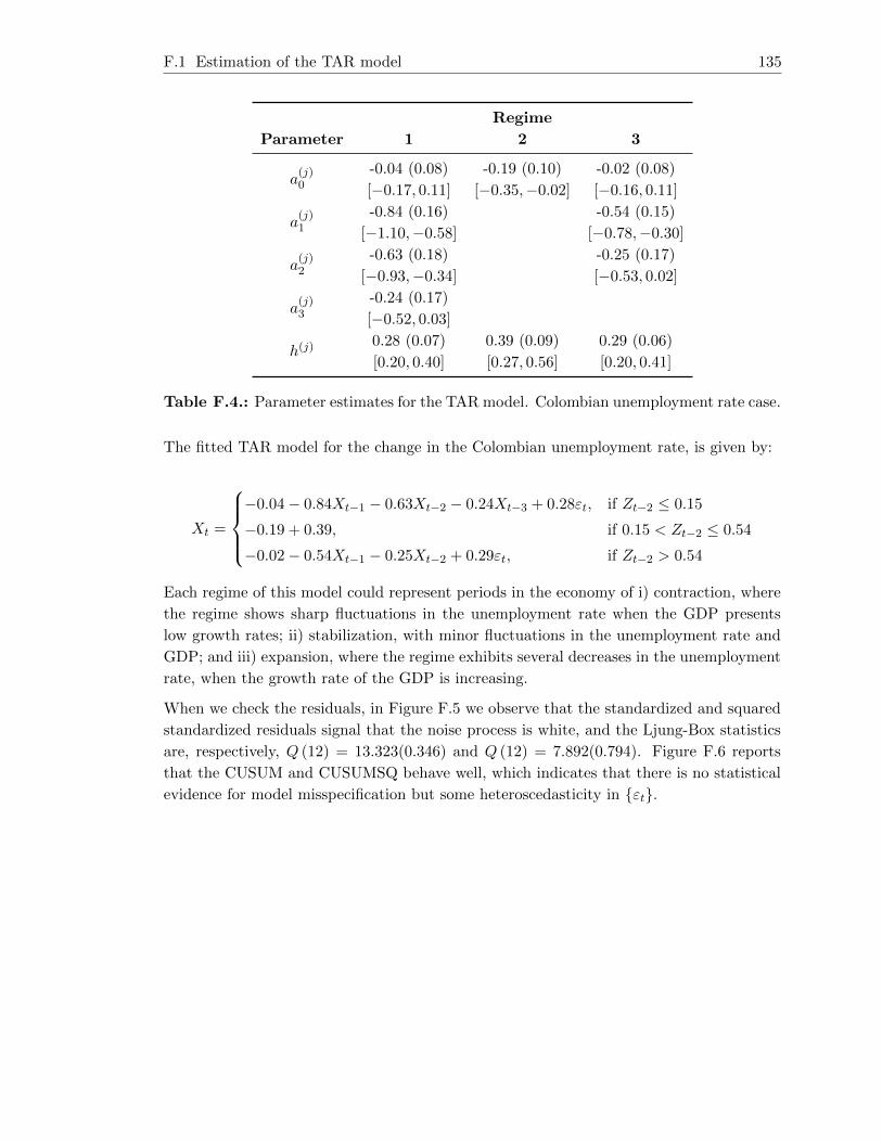
F.1 Estimation of the TAR model 135
Regime
Parameter 1 2 3
a(j)0
-0.04 (0.08)
[−0.17, 0.11]
-0.19 (0.10)
[−0.35,−0.02]
-0.02 (0.08)
[−0.16, 0.11]
a(j)1
-0.84 (0.16)
[−1.10,−0.58]
-0.54 (0.15)
[−0.78,−0.30]
a(j)2
-0.63 (0.18)
[−0.93,−0.34]
-0.25 (0.17)
[−0.53, 0.02]
a(j)3
-0.24 (0.17)
[−0.52, 0.03]
h(j)0.28 (0.07)
[0.20, 0.40]
0.39 (0.09)
[0.27, 0.56]
0.29 (0.06)
[0.20, 0.41]
Table F.4.: Parameter estimates for the TAR model. Colombian unemployment rate case.
The fitted TAR model for the change in the Colombian unemployment rate, is given by:
Xt =
−0.04− 0.84Xt−1 − 0.63Xt−2 − 0.24Xt−3 + 0.28εt, if Zt−2 ≤ 0.15
−0.19 + 0.39, if 0.15 < Zt−2 ≤ 0.54
−0.02− 0.54Xt−1 − 0.25Xt−2 + 0.29εt, if Zt−2 > 0.54
Each regime of this model could represent periods in the economy of i) contraction, where
the regime shows sharp fluctuations in the unemployment rate when the GDP presents
low growth rates; ii) stabilization, with minor fluctuations in the unemployment rate and
GDP; and iii) expansion, where the regime exhibits several decreases in the unemployment
rate, when the growth rate of the GDP is increasing.
When we check the residuals, in Figure F.5 we observe that the standardized and squared
standardized residuals signal that the noise process is white, and the Ljung-Box statistics
are, respectively, Q (12) = 13.323(0.346) and Q (12) = 7.892(0.794). Figure F.6 reports
that the CUSUM and CUSUMSQ behave well, which indicates that there is no statistical
evidence for model misspecification but some heteroscedasticity in {εt}.

F.2 Estimation of the SETAR model 136
Figure F.5.: Partial autocorrelation function of the fitted TAR model. (a) Standardized
residuals and (b) squared standardized residuals. Colombian unemployment
rate case.
Figure F.6.: (a) CUSUM and (b) CUSUMSQ charts for the residuals of the fitted TAR
model. Colombian unemployment rate case.
F.2. Estimation of the SETAR model
Based on the autocorrelation functions in Figure F.1 and the AIC and BIC criterion, we
identify p = 2 as the final autoregressive order to fit a SETAR model. Once we have
selected the autoregressive model, we check the nonlinearity of the series based on Tsay’s
(1989) test and find that with d = 2, where d is the delay parameter, it is obtained the
minimum p-value = 0.012 of the F statistic F = 4.594, rejecting the linearity of the series
at the 5% significance level.
Then, to determine the number of regimes and the threshold values, we use Figure F.7 that
shows the sequence of the t ratios of a lag-2 AR coefficient versus the threshold variable
Xt−2 in an arranged autoregression of order 2, and we identify that the data can be divided
into two regimes with a possible threshold at Xt−d = −0.4, because of the change on the
slope at approximately this point.
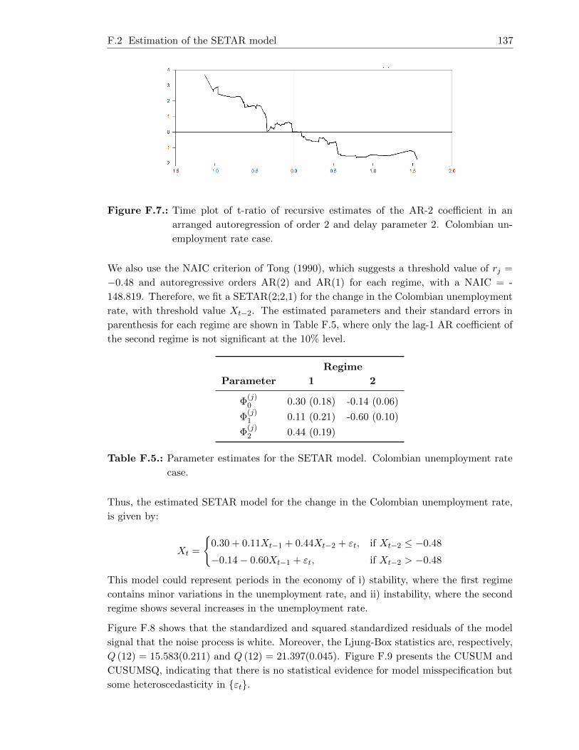
F.2 Estimation of the SETAR model 137
Figure F.7.: Time plot of t-ratio of recursive estimates of the AR-2 coefficient in an
arranged autoregression of order 2 and delay parameter 2. Colombian un-
employment rate case.
We also use the NAIC criterion of Tong (1990), which suggests a threshold value of rj =
−0.48 and autoregressive orders AR(2) and AR(1) for each regime, with a NAIC = -
148.819. Therefore, we fit a SETAR(2;2,1) for the change in the Colombian unemployment
rate, with threshold value Xt−2. The estimated parameters and their standard errors in
parenthesis for each regime are shown in Table F.5, where only the lag-1 AR coefficient of
the second regime is not significant at the 10% level.
Regime
Parameter 1 2
Φ(j)0 0.30 (0.18) -0.14 (0.06)
Φ(j)1 0.11 (0.21) -0.60 (0.10)
Φ(j)2 0.44 (0.19)
Table F.5.: Parameter estimates for the SETAR model. Colombian unemployment rate
case.
Thus, the estimated SETAR model for the change in the Colombian unemployment rate,
is given by:
Xt =
{0.30 + 0.11Xt−1 + 0.44Xt−2 + εt, if Xt−2 ≤ −0.48
−0.14− 0.60Xt−1 + εt, if Xt−2 > −0.48
This model could represent periods in the economy of i) stability, where the first regime
contains minor variations in the unemployment rate, and ii) instability, where the second
regime shows several increases in the unemployment rate.
Figure F.8 shows that the standardized and squared standardized residuals of the model
signal that the noise process is white. Moreover, the Ljung-Box statistics are, respectively,
Q (12) = 15.583(0.211) and Q (12) = 21.397(0.045). Figure F.9 presents the CUSUM and
CUSUMSQ, indicating that there is no statistical evidence for model misspecification but
some heteroscedasticity in {εt}.

F.3 Estimation of the STAR model 138
Figure F.8.: Partial autocorrelation function of the fitted SETAR model. (a) Standard-
ized residuals and (b) squared standardized residuals. Colombian unemploy-
ment rate case.
Figure F.9.: (a) CUSUM and (b) CUSUMSQ charts for the residuals of the fitted SETAR
model. Colombian unemployment rate case.
F.3. Estimation of the STAR model
We estimate the STAR model based on Section 1.3. With the identified p = 3 autoregressive
order, we evaluate the nonlinearity of the series based on Terasvirta’s (1994) test and find
that with a delay parameter of 1, d = 1, we obtain a p-value = 0.072 of the F statistic
F = 1.820, which rejects the linearity of the series.
Then, we choose between the LSTAR and the ESTAR models through a sequence of tests
of nested hypothesis (Terasvirta, 1994). We find that H01, H02 and H03 with F − stat =
0.648(0.586), F − stat = 2.407(0.071) and F − stat = 2.365(0.074) respectively, are not
rejected at the 5% significance level (the p-values are in parenthesis). Thus, the model we
choose is the LSTAR.
In Table F.6, we show the estimates for the parameters and their respective standard error
in parenthesis, where all estimates, except the parameter γ and c, are significant at the 5%
level.
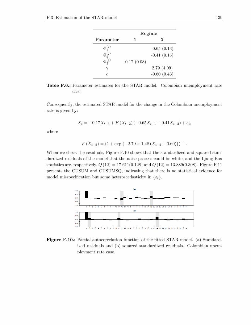
F.3 Estimation of the STAR model 139
Regime
Parameter 1 2
Φ(j)1 -0.65 (0.13)
Φ(j)2 -0.41 (0.15)
Φ(j)3 -0.17 (0.08)
γ 2.79 (4.09)
c -0.60 (0.43)
Table F.6.: Parameter estimates for the STAR model. Colombian unemployment rate
case.
Consequently, the estimated STAR model for the change in the Colombian unemployment
rate is given by:
Xt = −0.17Xt−3 + F (Xt−2) (−0.65Xt−1 − 0.41Xt−2) + εt,
where
F (Xt−2) = (1 + exp {−2.79× 1.48 (Xt−2 + 0.60)})−1 .
When we check the residuals, Figure F.10 shows that the standardized and squared stan-
dardized residuals of the model that the noise process could be white, and the Ljung-Box
statistics are, respectively, Q (12) = 17.611(0.128) and Q (12) = 13.889(0.308). Figure F.11
presents the CUSUM and CUSUMSQ, indicating that there is no statistical evidence for
model misspecification but some heteroscedasticity in {εt}.
Figure F.10.: Partial autocorrelation function of the fitted STAR model. (a) Standard-
ized residuals and (b) squared standardized residuals. Colombian unem-
ployment rate case.

F.4 Estimation of the MSAR model 140
Figure F.11.: (a) CUSUM and (b) CUSUMSQ charts for the residuals of the fitted STAR
model. Colombian unemployment rate case.
F.4. Estimation of the MSAR model
Based on Section 1.4, we estimate the MSAR model. Table F.7 shows the estimates of the
parameters of the model and their respective standard errors in parenthesis.
state
Parameter 1 2
Φ(j)0 -0.03 (0.05) -0.19 (0.22)
Φ(j)1 -0.44 (0.14) -0.61 (0.24)
Φ(j)2 -0.11 (0.15) -0.24 (0.28)
Table F.7.: Parameter estimates for the MSAR model. Colombian unemployment rate
case.
Therefore, the estimated MSAR model for the change in the Colombian unemployment
rate is given by:
Xt =
{−0.03− 0.44Xt−1 − 0.11Xt−2 + ε1t, if st = 1
−0.19− 0.61Xt−1 − 0.24Xt−2 + ε2t, if st = 2
The conditional mean of Xt for regime 1 is -0.02 and for regime 2 is -0.12. Hence, the
first state represents the stable periods in the Colombian economy, with no considerable
movements in the unemployment rate, and the second state represents the expansionary
periods with more decreases in this economic time series53.
When we evaluate this model, Figure F.12 shows that the standardized and squared stan-
dardized residuals signal that the noise process could be white, and the Ljung-Box statistics
53 The probabilities of moving from one state to the other are p (st = 2|st = 1) = 0.93(0.05) and
p (st = 1|st = 2) = 0.28(0.15), where the number in parenthesis is the standard error. Additionally,
the unconditional probability that the process is in regime 1 is 0.79 and that it is in regime 2 is 0.21.
The coefficients allow us to know that the probability that expansion is followed by another expansion
period is p (1, 1) = 0.93, and that the probability that contraction is followed by another contraction
period is p (2, 2) = 0.92.

F.5 Estimation of the AR model 141
are, respectively, Q (12) = 18.921(0.090) and Q (12) = 15.483(0.216). Figure F.13 presents
the CUSUM and CUSUMSQ, indicating that there is statistical evidence for model mis-
specification and heteroscedasticity in {εt}.
Figure F.12.: Partial autocorrelation function of the fitted MSAR model. (a) Standard-
ized residuals and (b) squared standardized residuals. Colombian unem-
ployment rate case.
Figure F.13.: (a) CUSUM and (b) CUSUMSQ charts for the residuals of the fitted MSAR
model. Colombian unemployment rate case.
F.5. Estimation of the AR model
We estimate an AR(2) model for the change in the Colombian unemployment rate54:
(1 + +0.56B + 0.16B2
)Xt = at, σ2a = 0.3,
The standard error of both coefficients is 0.09. Figure F.14 shows that the standardized
residuals and the squared standardized residuals signal that the noise process could be
white. Fourthermore, the Ljung-Box statistics are, respectively, Q (12) = 18.098(0.113)
and Q (12) = 13.589(0.328). Figure F.15 shows the CUSUM and CUSUMSQ, indicating
54 As reported by the Augmented Dickey-Fuller (ADF) (p−value = 0.000), Phillips Perron (PP) (p−value =
0.000) and Kwiatkowski-Phillips-Schmidt-Shin (KPSS) (Test statistic = 0.085 and Critical value =
0.463, the growth rate of the Colombian unemployment rate is stationary at the 5% significance level.

F.5 Estimation of the AR model 142
that there is no statistical evidence for model misspecification but some heteroscedasticity
in {εt}.
Figure F.14.: Partial autocorrelation function of the fitted AR model. (a) Standardized
residuals and (b) squared standardized residuals. Colombian unemploy-
ment rate case.
Figure F.15.: (a) CUSUM and (b) CUSUMSQ charts for the residuals of the fitted AR
model. Colombian unemployment rate case.

Appendix G
General review of the model estimation for theannual growth rate of the Colombian GDP
G.1. Estimation of the TAR model
We use as the variable of interest the annual growth rate of the ISE, as a proxi of the
GDP, and as the threshold variable we use the Colombian spread term defined in Section
3.2. Figure G.1 and Figure G.2 show that both series have significant autocorrelations for
a large number of lags.
Figure G.1.: (a) Sample autocorrelation function and (b) sample partial autocorrelation
function for the annual growth rate of Colombian GDP.

G.1 Estimation of the TAR model 144
Figure G.2.: (a) Sample autocorrelation function and (b) sample partial autocorrelation
function for the Colombian spread term.
Then, we test the null hypothesis of AR linearity against the alternative of bivariate TAR
nonlinearity. Under the AIC criterion, we found that k = 2 is a reasonable autoregressive
order for Xt. Under the null hypothesis, the results of the test let us define as the delay
parameter of 5 for the threshold variable, thus, the input variable for the dynamic system
is Zt−5.
Figure G.3 shows the annual growth rate of the Colombian GDP and the spread term from
2003:06 to 2012:06. The shading areas denote the business cycle contractions from peak
to trough based on Alfonso et al. (2012).
Figure G.3.: (a) Time plot of the annual growth rate of Colombian GDP and (b) Time
plot of the Colombian spread term.
We specify the maximum number of regimes l0 by means of a regression function between
Xt and Zt, that is estimated using a nonparametric kernel approach and that is presented
in Figure G.4. We observe that 3 could be postulated as the possible maximum regimes
for the TAR model.

G.1 Estimation of the TAR model 145
Figure G.4.: Nonparametric regression between the annual growth rate of the Colombian
GDP (X) and Colombian spread term (Z).
Next, to specify the prior densities for the nonstructural parameters, we define the prior
densities for θx where θ0,j = 0, V −10,j = 0.01I with I the identity matrix, γ0,j = 1.5 and
β0,j = σ2
2 with j = 1, 2, 3 and σ2 = 0.871 that is the residual variance of the AR(2) that
was fitted to the annual growth rate of the ISE. The maximum autoregressive order for all
regimes is k = 2, the same value fitted to the variable of interest. The prior distributions for
both the number of regimes and the autoregressive orders that we use in the identification
of l are π2 = π3 = 0.5 and p (kil|l) = 0.333 for kil = 0, 1, 2; i = 1, .., l, respectively.
Then, to look for the location of thresholds in each possible regime, we choose the per-
centiles 5k where k = 1, 2, . . . , 19, with respective values -3.82, -3.70, -3.44, -3.20, -2.75,
-2.33, -2.01, -1.24, -1.02, -0.34, -0.03, 0.04, 0.30, 0.49, 0.66, 0.79, 0.96, 1.08, 1.28. The pos-
sible thresholds and autoregressive orders for each possible regime are presented in Table
G.1.
` Thresholds Autoregressive orders Minimum NAIC
2 -0.34 1, 1 3.25830
3 -3.20 -0.34 1, 1, 1 2.80465
Table G.1.: Set of possible number of regimes for the real data. Colombian GDP case.
With those possible thresholds and the information mentioned above, we compute the
posterior probability distribution for the number of regimes. 3000 iterates were generate,
with a burn-in point of 10% of the draws55. The results showed in Table G.2 allow us to
set l = 3 as the appropriate number of regimes.
55 The convergence of the Gibbs sampler was checked via the stationarity approach, where it was observed
that the sample autocorrelation functions of the sequences{p(i)l
}for l = 2, 3 decay quickly.

G.1 Estimation of the TAR model 146
` p`
2 0.3062
3 0.6938
Table G.2.: Posterior probability function for the number of regimes for the real data.
Colombian GDP case.
Thus, conditional on l = 3, we estimate the autoregressive orders for k1, k2 and k3. Based
on Table G.3, the identified autoregressive orders are k1 = 2, k2 = 2 and k3 = 2. As before,
convergence of the Gibbs sampler was checked via stationarity, and for 5000 iterates with a
burn-in point of 10% of the draws, it is observed that the sample autocorrelations functions
decay quickly56.
Regime
Autoregressive
Order1 2 3
0 1.54×10⁻¹¹ 1.01×10−50 1.87×10⁻³⁵
1 0.2140 0.1537 0.0597
2 0.7860 0.8463 0.9403
Table G.3.: Posterior probabilities for the autoregressive orders in the real data. Colom-
bian GDP case.
Consequently, we fit a TAR(3;2,2,2) with thresholds values r1 = −3.20 and r2 = −0.34,
which respectively are the 20th and 50th percentiles of the spread term. Table G.4 shows
the estimates for the nonstructural parameters, with their respective posterior standard
error in parenthesis and 90% credible interval in brackets57. These results show that not all
the coefficients are significant at the 5% level. However, we decide to estimate the model
with all the coefficients, given that that improves the final estimation.
56 We performed a sensibility analysis where we changed the prior densities of the autoregressive orders
and the nonstructural parameters, and we found that the estimated autoregressive orders are the same
for different priors of the nonstructural parameters and for different priors of the autoregressive orders.57 5000 iterates were generated, with a burn-in point of 10% of the draws, and it was found that the
autocorrelation functions for all the parameters decay quickly, indicating the convergence of the Gibbs
sampler.

G.1 Estimation of the TAR model 147
Regime
Parameter 1 2 3
a(j)0
0.20 (0.47)
[−0.57, 0.98]
0.64 (0.40)
[−0.04, 1.28]
1.43 (0.53)
[0.56, 2.29]
a(j)1
0.70 (0.22)
[0.34, 1.05]
0.73 (0.17)
[0.44, 1.01]
0.51 (0.14)
[0.28, 0.74]
a(j)2
0.18 (0.22)
[−0.18, 0.53]
0.17 (0.17)
[−0.12, 0.45]
0.20 (0.13)
[−0.02, 0.42]
h(j)1.51 (0.51)
[0.89, 2.44]
0.41 (0.11)
[0.27, 0.61]
0.94 (0.19)
[0.67, 1.28]
Table G.4.: Parameter estimates for the TAR model. Colombian GDP case.
The fitted TAR model for the annual growth rate of the Colombian GDP is given by:
Xt =
0.20 + 0.70Xt−1 + 0.18Xt−2 + 1.51εt, if Zt−5 ≤ −3.20
0.64 + 0.73Xt−1 + 0.17Xt−2 + 0.41εt, if −3.20 < Zt−5 ≤ −0.34
1.43 + 0.51Xt−1 + 0.20Xt−2 + 0.94εt, if Zt−5 > −0.34
This model could represent periods in the economy of i) contraction, given that this regime
presents the lowest values of the growth rate of the real GDP, when spreads are low due to
contractionary monetary policies; ii) transition, where the regime has minor but positive
fluctuations in the growth rate of the real GDP; during a stable behavior of the spread
term and iii) expansion, where this last regime is associated with the important increases
in the growth rate of real GDP, when the monetary policy is expansioning.
When we check the residuals, in Figure G.5 we observe that the standardized and squared
standardized residuals slightly signal that some nonlinear structure in the data is not ex-
plained by the model, and the Ljung-Box statistics are, respectively, Q (12) = 27.613(0.006)
and Q (12) = 18.715(0.095). Figure G.6 shows that the CUSUM and CUSUMSQ behave
well, which indicates that there is neither statistical evidence for model misspecification
nor heteroscedasticity in {εt}.
Figure G.5.: Partial autocorrelation function of the fitted TAR model. (a) Standardized
residuals and (b) squared standardized residuals. Colombian GDP case.

G.2 Estimation of the SETAR model 148
Figure G.6.: (a) CUSUM and (b) CUSUMSQ charts for the residuals of the fitted TAR
model. Colombian GDP case.
G.2. Estimation of the SETAR model
Based on the autocorrelation functions in Figure G.1 and the AIC and BIC criterion, we
identify p = 2 as the final autoregressive order to fit a SETAR model. Under the Tsay’s
(1989) test and find that with d = 4, it is obtained the minimum p-value = 0.0279 of the
F statistic F = 3.711, rejecting the linearity of the series at the 5% significance level.
Figure G.7 shows the sequence of the t ratios of a lag-2 AR coefficient versus the threshold
variable Xt−d in an arranged autoregression of order 2, and we identify that the data can
be divided into two regimes with a possible threshold at Xt−d = 3.0, because of the change
on the slope at approximately this point.
Figure G.7.: Time plot of t-ratio of recursive estimates of the AR-2 coefficient in an
arranged autoregression of order 2 and delay parameter 4. Colombian GDP
case.
We also use the NAIC criterion of Tong (1990), which suggests a threshold value of rj = 3.19
and autoregressive orders AR(1) and AR(2) for each regime, with a NAIC = -12.958. Based
on that, we fit a SETAR(2;1,2) for the annual growth rate of the GDP, with threshold value
Xt−4. The estimated parameters and their standard errors in parenthesis for each regime
are shown in Table G.5, where all estimates are significant at the 5% level.

G.2 Estimation of the SETAR model 149
Regime
Parameter 1 2
Φ(j)1 1.04 (0.05) 0.67 (0.12)
Φ(j)2 0.67 (0.12) 0.31 (0.12)
Table G.5.: Parameter estimates for the SETAR model. Colombian GDP case.
Thus, the estimated SETAR model for the annual growth rate of the Colombian GDP is
given by:
Xt =
{1.04Xt−1 + εt, if Xt−4 ≤ 3.19
0.67Xt−1 + 0.31Xt−2 + εt, if Xt−4 > 3.19
This model could represent periods in the economy of i) stability, where the first regime
contains the minor increases in the growth rate of the real GDP, and ii) expansion, where
the second regime shows the greatest increases in the growth rate of the real GDP.
Figure G.8 shows that the standardized and squared standardized residuals of the model
slightly signal that some nonlinear structure in the data is not explained by the model. The
Ljung-Box statistics are, respectively, Q (12) = 29.561(0.003) and Q (12) = 22.395(0.033).
Figure G.9 presents the CUSUM and CUSUMSQ, which indicate that there is no statistical
evidence for model misspecification but some heteroscedasticity in {εt}.
Figure G.8.: Partial autocorrelation function of the fitted SETAR model. (a) Standard-
ized residuals and (b) squared standardized residuals. Colombian GDP
case.

G.3 Estimation of the STAR model 150
Figure G.9.: (a) CUSUM and (b) CUSUMSQ charts for the residuals of the fitted SETAR
model. Colombian GDP case.
G.3. Estimation of the STAR model
With an identified p = 13 autoregressive order, we evaluate the nonlinearity of the series
based on Terasvirta’s (1994) test and find that, with a delay parameter of d = 13, we
obtain the p-value = 0.0064 for the F statistic F = 2.1967, which rejects the linearity of
the series.
When we compute the tests of nested hypothesis of Terasvirta (1994), we find that at the
10% significance level, H01 is rejected, while H02 and H03 are not, where the respective
p-value is 0.0018, 0.2014 and 0.6787. These results suggest that we must estimate a LSTAR
model.
Table G.6 shows the estimates for the parameters and their respective standard error in
parenthesis, where only the lag-4 AR coefficient of the second regime and the parameter γ
are not significant at the 5% level.
Regime
Parameter 1 2
Φ(j)0 0.90 (0.38)
Φ(j)1 0.40 (0.16) 0.35 (0.16)
Φ(j)2 0.31 (0.11)
Φ(j)4 -0.15 (0.10)
Φ(j)9 0.46 (0.17) -0.42 (0.18)
Φ(j)12 -0.36 (0.09)
Φ(j)13 0.23 (0.10)
γ 11.49 (17.76)
c 3.98 (0.30)
Table G.6.: Parameter estimates for the STAR model. Colombian GDP case.
Consequently, the estimated STAR model for the annual growth rate of the Colombian
GDP is given by:

G.4 Estimation of the MSAR model 151
Xt = 0.90 + 0.40Xt−1 + 0.43Xt−2 + 0.46Xt−9 − 0.36Xt−12
+ F (Xt−13) (0.35Xt−1 − 0.15Xt−4 − 0.42Xt−9 + 0.23Xt−13) + εt,
where
F (Xt−13) = (1 + exp {−11.49 (Xt−13 − 3.98)})−1 .
When we check the residuals, Figure G.10 shows that the standardized and squared stan-
dardized residuals of the model signal that the noise process is white, and the Ljung-Box
statistics are, respectively, Q (12) = 13.437(0.338) and Q (12) = 5.006(0.958). Figure
G.11 presents the CUSUM and CUSUMSQ, which indicate that there is neither statistical
evidence for model misspecification nor heteroscedasticity in {εt}.
Figure G.10.: Partial autocorrelation function of the fitted STAR model. (a) Standard-
ized residuals and (b) squared standardized residuals. Colombian GDP
case.
Figure G.11.: (a) CUSUM and (b) CUSUMSQ charts for the residuals of the fitted STAR
model. Colombian GDP case.
G.4. Estimation of the MSAR model
Table G.7 shows the estimates of the parameters of the model and their respective standard
errors in parenthesis.

G.4 Estimation of the MSAR model 152
state
Parameter 1 2
Φ(j)0 -0.32 (0.10) 0.83 (0.34)
Φ(j)1 0.71 (0.04) 0.71 (0.11)
Φ(j)2 0.64 (0.05) 0.16 (0.13)
Φ(j)3 -0.51 (0.04) -0.04 (0.14)
Φ(j)5 0.31 (0.04) -0.02 (0.10)
Table G.7.: Parameter estimates for the MSAR model. Colombian GDP case.
Therefore, the estimated MSAR model for the annual growth rate of the Colombian GDP
is given by:
Xt =
{−0.32 + 0.71Xt−1 + 0.64Xt−2 − 0.51Xt−3 + 0.31Xt−5 + ε1t, if st = 1
0.83 + 0.71Xt−1 + 0.16Xt−2 − 0.04Xt−3 − 0.02Xt−5 + ε2t, if st = 2
The conditional mean of Xt for regime 1 is -1.09 and for regime 2 is 2.89. The sample
variances of ε1t and ε2t are 0.01 and 0.97, respectively58. Hence, the first state could
represent unstable periods with minor increases in the real output, and the second state
represents a stable economy with strong increases I the real output.
When we check this model, Figure G.12 shows that the standardized and squared standard-
ized residuals of the model signal that the noise process is white. Moreover, the Ljung-Box
statistics are, respectively, Q (12) = 12.068(0.440) and Q (12) = 4.225(0.979). Figure G.13
presents the CUSUM and CUSUMSQ, which indicate that there is statistical evidence for
model misspecification and some heteroscedasticity in {εt}.
Figure G.12.: Partial autocorrelation function of the fitted MSAR model. (a) Standard-
ized residuals and (b) squared standardized residuals. Colombian GDP
case.
58 The probabilities of moving from one state to the other are p (st = 2|st−1 = 1) = 0.59(0.15) and
p (st = 1|st−1 = 2) = 0.17(0.07), where the number in parenthesis is the standard error. Addition-
ally, the unconditional probability that the process is in regime 1 is 0.22 and that it is in regime 2 is
0.78.
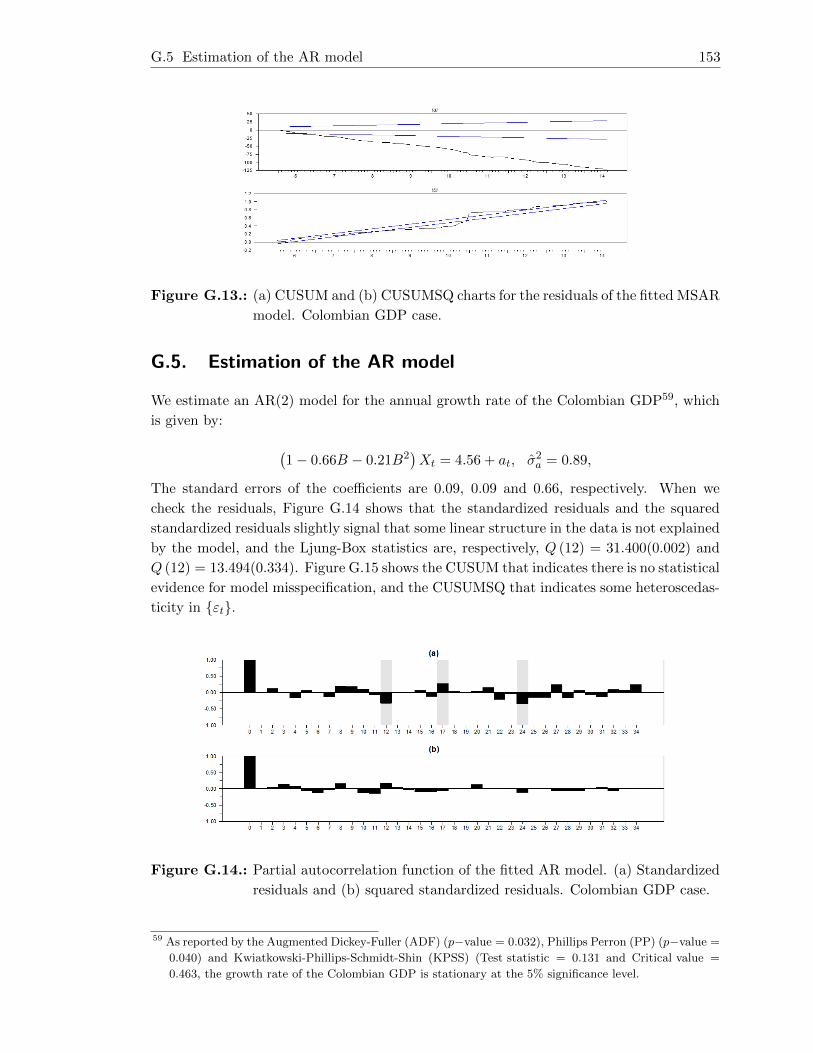
G.5 Estimation of the AR model 153
Figure G.13.: (a) CUSUM and (b) CUSUMSQ charts for the residuals of the fitted MSAR
model. Colombian GDP case.
G.5. Estimation of the AR model
We estimate an AR(2) model for the annual growth rate of the Colombian GDP59, which
is given by:
(1− 0.66B − 0.21B2
)Xt = 4.56 + at, σ2a = 0.89,
The standard errors of the coefficients are 0.09, 0.09 and 0.66, respectively. When we
check the residuals, Figure G.14 shows that the standardized residuals and the squared
standardized residuals slightly signal that some linear structure in the data is not explained
by the model, and the Ljung-Box statistics are, respectively, Q (12) = 31.400(0.002) and
Q (12) = 13.494(0.334). Figure G.15 shows the CUSUM that indicates there is no statistical
evidence for model misspecification, and the CUSUMSQ that indicates some heteroscedas-
ticity in {εt}.
Figure G.14.: Partial autocorrelation function of the fitted AR model. (a) Standardized
residuals and (b) squared standardized residuals. Colombian GDP case.
59 As reported by the Augmented Dickey-Fuller (ADF) (p−value = 0.032), Phillips Perron (PP) (p−value =
0.040) and Kwiatkowski-Phillips-Schmidt-Shin (KPSS) (Test statistic = 0.131 and Critical value =
0.463, the growth rate of the Colombian GDP is stationary at the 5% significance level.

G.5 Estimation of the AR model 154
Figure G.15.: (a) CUSUM and (b) CUSUMSQ charts for the residuals of the fitted AR
model. Colombian GDP case.
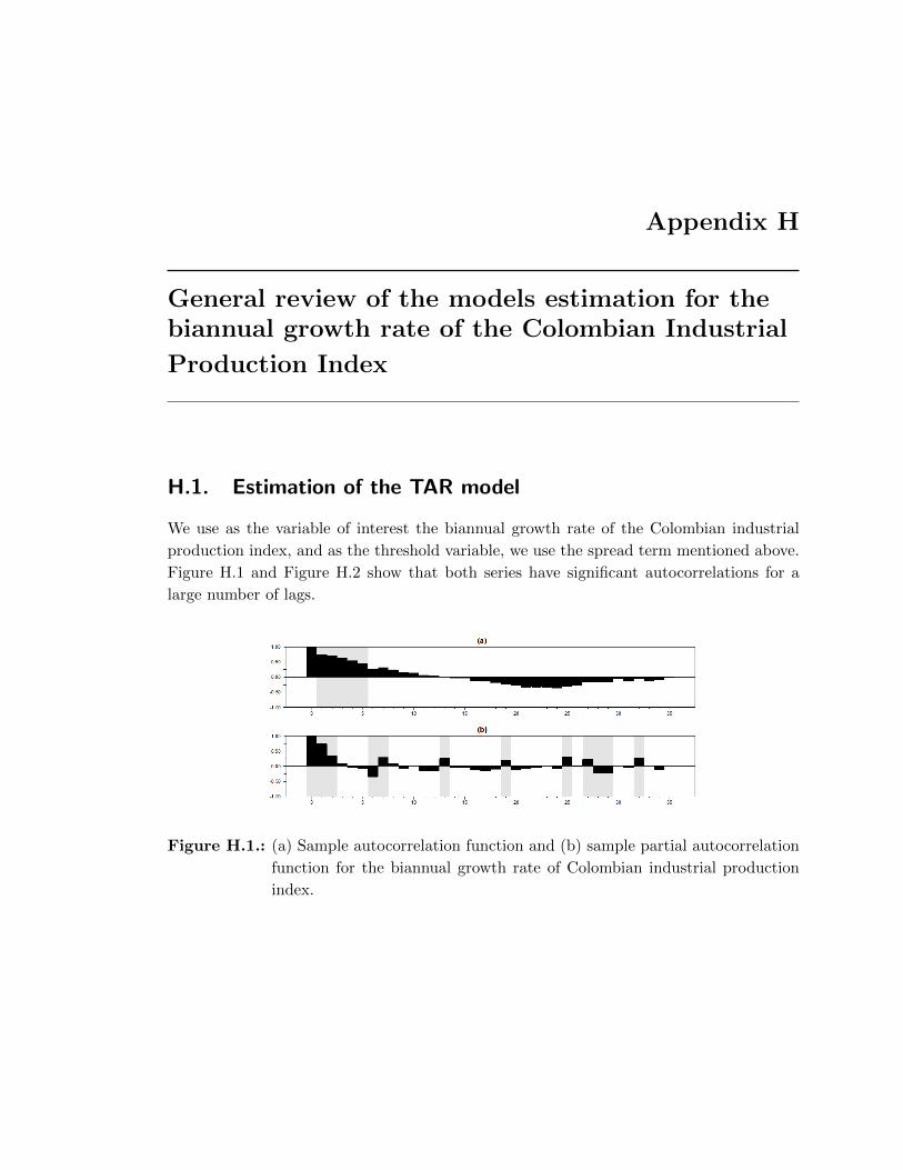
Appendix H
General review of the models estimation for thebiannual growth rate of the Colombian Industrial
Production Index
H.1. Estimation of the TAR model
We use as the variable of interest the biannual growth rate of the Colombian industrial
production index, and as the threshold variable, we use the spread term mentioned above.
Figure H.1 and Figure H.2 show that both series have significant autocorrelations for a
large number of lags.
Figure H.1.: (a) Sample autocorrelation function and (b) sample partial autocorrelation
function for the biannual growth rate of Colombian industrial production
index.
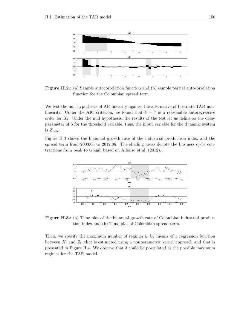
H.1 Estimation of the TAR model 156
Figure H.2.: (a) Sample autocorrelation function and (b) sample partial autocorrelation
function for the Colombian spread term.
We test the null hypothesis of AR linearity against the alternative of bivariate TAR non-
linearity. Under the AIC criterion, we found that k = 7 is a reasonable autoregressive
order for Xt. Under the null hypothesis, the results of the test let us define as the delay
parameter of 5 for the threshold variable, thus, the input variable for the dynamic system
is Zt−5.
Figure H.3 shows the biannual growth rate of the industrial production index and the
spread term from 2003:06 to 2012:06. The shading areas denote the business cycle con-
tractions from peak to trough based on Alfonso et al. (2012).
Figure H.3.: (a) Time plot of the biannual growth rate of Colombian industrial produc-
tion index and (b) Time plot of Colombian spread term.
Then, we specify the maximum number of regimes l0 by means of a regression function
between Xt and Zt, that is estimated using a nonparametric kernel approach and that is
presented in Figure H.4. We observe that 3 could be postulated as the possible maximum
regimes for the TAR model.

H.1 Estimation of the TAR model 157
Figure H.4.: Nonparametric regression between the biannual growth rate of Colombian
industrial production (X) and Colombian spread term (Z).
Then, to specify the prior densities for the nonstructural parameters, we define the prior
densities for θx where θ0,j = 0, V −10,j = 0.01I with I the identity matrix, γ0,j = 1.5 and
β0,j = σ2
2 with j = 1, 2, 3 and σ2 = 3.809 that is the residual variance of the AR(7) that
was fitted to the biannual growth rate of the industrial production index. The maximum
autoregressive order for all regimes is k = 7, the same value fitted to the variable of
interest. The prior distributions for both the number of regimes and the autoregressive
orders that we use in the identification of l are π2 = π3 = 0.5 and p (kil|l) = 0.125 for
kil = 0, 1, . . . , 7; i = 1, .., l, respectively.
Then, to look for the location of thresholds in each possible regime, we choose the per-
centiles 5k where k = 1, 2, . . . , 19, with respective values -3.82, -3.70, -3.44, -3.20, -2.75,
-2.33, -2.01, -1.24, -1.02, -0.34, -0.03, 0.04, 0.30, 0.49, 0.66, 0.79, 0.96, 1.08, 1.28. The pos-
sible thresholds and autoregressive orders for each possible regime are presented in Table
H.1.
` Thresholds Autoregressive orders Minimum NAIC
2 -0.34 1, 1 4.96476
3 -1.02 -0.03 7, 7, 7 4.38697
Table H.1.: Set of possible number of regimes for the real data. Colombian indpro case.
With those possible thresholds and the information mentioned above, we compute the
posterior probability distribution for the number of regimes. 3000 iterates were generated
with a burn-in point of 10% of the draws60. The results showed in Table H.2 allow us to
set =3 as the appropriate number of regimes.
60 The convergence of the Gibbs sampler was checked via the stationarity approach, where it was observed
that the sample autocorrelation functions of the sequences{p(i)l
}for l = 2, 3 decay quickly.
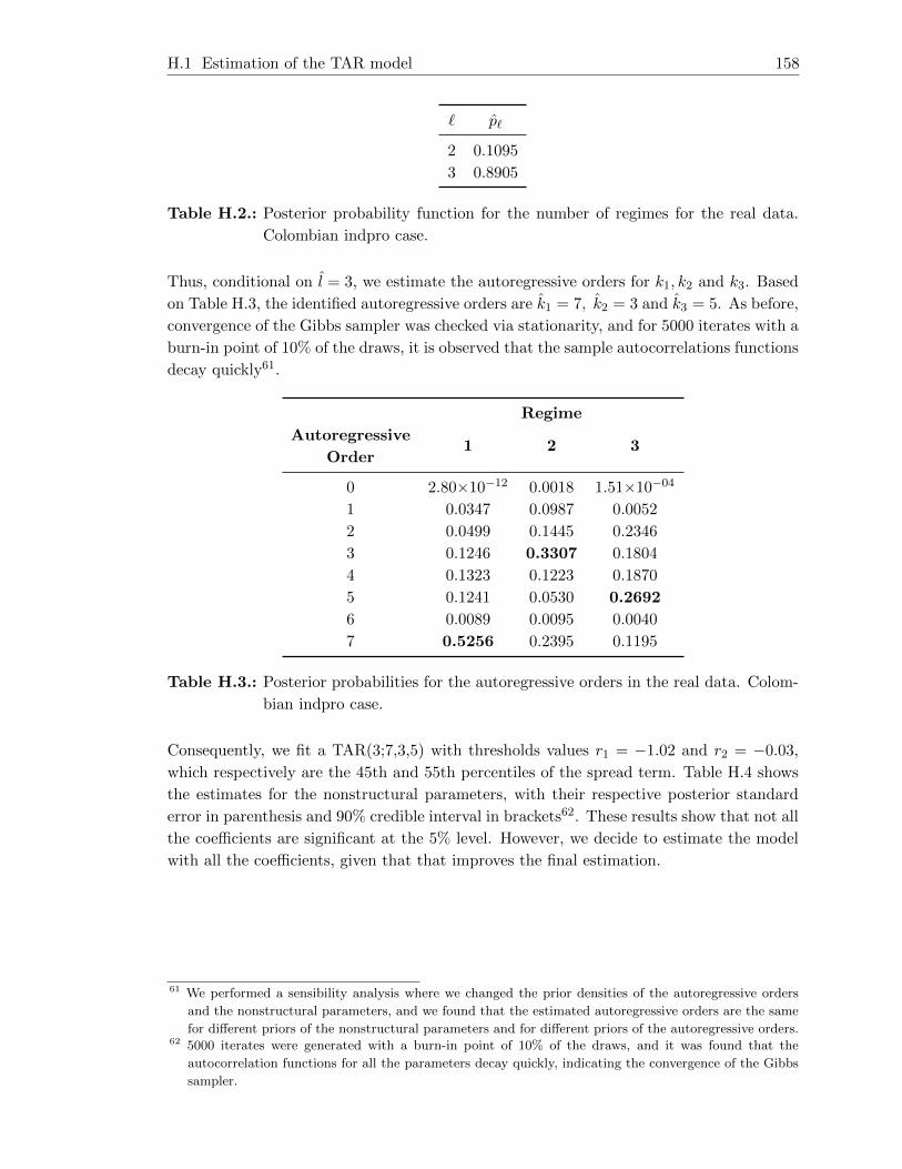
H.1 Estimation of the TAR model 158
` p`
2 0.1095
3 0.8905
Table H.2.: Posterior probability function for the number of regimes for the real data.
Colombian indpro case.
Thus, conditional on l = 3, we estimate the autoregressive orders for k1, k2 and k3. Based
on Table H.3, the identified autoregressive orders are k1 = 7, k2 = 3 and k3 = 5. As before,
convergence of the Gibbs sampler was checked via stationarity, and for 5000 iterates with a
burn-in point of 10% of the draws, it is observed that the sample autocorrelations functions
decay quickly61.
Regime
Autoregressive
Order1 2 3
0 2.80×10⁻¹² 0.0018 1.51×10−04
1 0.0347 0.0987 0.0052
2 0.0499 0.1445 0.2346
3 0.1246 0.3307 0.1804
4 0.1323 0.1223 0.1870
5 0.1241 0.0530 0.2692
6 0.0089 0.0095 0.0040
7 0.5256 0.2395 0.1195
Table H.3.: Posterior probabilities for the autoregressive orders in the real data. Colom-
bian indpro case.
Consequently, we fit a TAR(3;7,3,5) with thresholds values r1 = −1.02 and r2 = −0.03,
which respectively are the 45th and 55th percentiles of the spread term. Table H.4 shows
the estimates for the nonstructural parameters, with their respective posterior standard
error in parenthesis and 90% credible interval in brackets62. These results show that not all
the coefficients are significant at the 5% level. However, we decide to estimate the model
with all the coefficients, given that that improves the final estimation.
61 We performed a sensibility analysis where we changed the prior densities of the autoregressive orders
and the nonstructural parameters, and we found that the estimated autoregressive orders are the same
for different priors of the nonstructural parameters and for different priors of the autoregressive orders.62 5000 iterates were generated with a burn-in point of 10% of the draws, and it was found that the
autocorrelation functions for all the parameters decay quickly, indicating the convergence of the Gibbs
sampler.
H.1 Estimation of the TAR model 159
Regime
Parameter 1 2 3
a(j)0
0.14 (0.32)
[−0.39, 0.66]
-0.67 (1.34)
[−2.89, 1.47]
1.26 (0.63)
[0.22, 2.29]
a(j)1
0.73 (0.15)
[0.48, 0.97]
0.67 (0.39)
[0.03, 1.30]
0.17 (0.17)
[−0.11, 0.45]
a(j)2
0.09 (0.16)
[−0.18, 0.35]
0.16 (0.36)
[−0.42, 0.72]
0.34 (0.18)
[0.04, 0.63]
a(j)3
0.40 (0.16)
[0.14, 0.67]
0.18 (0.38)
[−0.42, 0.80]
0.04 (0.19)
[−0.26, 0.34]
a(j)4
-0.21 (0.16)
[−0.47, 0.06]
-0.04 (0.18)
[−0.33, 0.25]
a(j)5
0.12 (0.16)
[−0.14, 0.37]
-0.04 (0.16)
[−0.31, 0.22]
a(j)6
-0.62 (0.16)
[−0.89,−0.35]
a(j)7
0.38 (0.16)
[0.12, 0.64]
h(j)4.61 (1.05)
[3.20, 6.57]
6.00 (3.71)
[2.53, 12.70]
4.26 (0.99)
[2.92, 6.09]
Table H.4.: Parameter estimates for the TAR model. Colombian indpro case.
Thus, the fitted TAR model for the biannual growth rate of the Colombian industrial
production index is given by:
Xt =
0.14 + 0.73Xt−1 + 0.09Xt−2 + 0.40Xt−3 − 0.21Xt−4
+0.12Xt−5 − 0.62Xt−6 + 0.38Xt−7 + 4.61εt, if Zt−5 ≤ −1.02
−0.67 + 0.67Xt−1 + 0.16Xt−2 + 0.18Xt−3 + 6.00εt, if −1.02 < Zt−5 ≤ −0.03
1.26 + 0.17Xt−1 + 0.34Xt−2 + 0.04Xt−3 − 0.04Xt−4
−0.04Xt−5 + 4.26εt, if Zt−5 > −0.03
This model could represent periods in the economy of i) contraction, given that this regime
contains the greatest decreases in the growth rate of the industrial production index, when
there is a low spread due to contractionary monetary policies; ii) stabilization, where the
regime shows minor increases in the growth rate of the industrial production index; and
iii) expansion, where the regime exhibits the greatest increases in the growth rate of the
industrial production index, when there is high spread because of expansionary monetary
policies.
When we check the residuals, in Figure H.5 it is observed that the standardized residu-
als and squared standardized residuals of the model signal that the noise process could
be white, and the Ljung-Box statistics are, respectively, Q (12) = 11.647(0.474) and
Q (12) = 16.512(0.169). Figure H.6 reports that the CUSUM and CUSUMSQ behave

H.2 Estimation of the SETAR model 160
well, which indicates that there is neither statistical evidence for model misspecification
nor heteroscedasticity in {εt}.
Figure H.5.: Partial autocorrelation function of the fitted TAR model. (a) Standardized
residuals and (b) squared standardized residuals. Colombian indpro case.
Figure H.6.: (a) CUSUM and (b) CUSUMSQ charts for the residuals of the fitted TAR
model. Colombian indpro case.
H.2. Estimation of the SETAR model
Based on the autocorrelation functions in Figure H.1 and the AIC and BIC criterion, we
identify p = 3 as the final autoregressive order to fit a SETAR model. Once we select the
autoregressive model, we check the nonlinearity of the series based on Tsay’s (1989) test
and find that with d = 2, it is obtained the minimum p-value = 0.0352 of the F statistic
F = 2.696, rejecting the linearity of the series at the 5% significance level.
Figure H.7 shows the sequence of the t ratios of a lag-2 AR coefficient versus the threshold
variable Xt−d in an arranged autoregression of order 3, and we identify that the data can
be divided into two regimes with a possible threshold at Xt−d = −0.5, because of the
change on the slope at approximately this point.
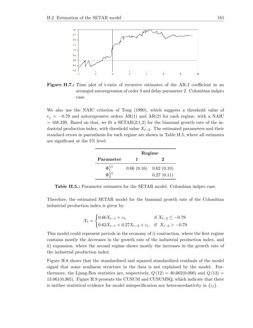
H.2 Estimation of the SETAR model 161
Figure H.7.: Time plot of t-ratio of recursive estimates of the AR-2 coefficient in an
arranged autoregression of order 3 and delay parameter 2. Colombian indpro
case.
We also use the NAIC criterion of Tong (1990), which suggests a threshold value of
rj = −0.79 and autoregressive orders AR(1) and AR(2) for each regime, with a NAIC
= 168.239. Based on that, we fit a SETAR(2;1,2) for the biannual growth rate of the in-
dustrial production index, with threshold value Xt−2. The estimated parameters and their
standard errors in parenthesis for each regime are shown in Table H.5, where all estimates
are significant at the 5% level.
Regime
Parameter 1 2
Φ(j)1 0.66 (0.16) 0.62 (0.10)
Φ(j)2 0.27 (0.11)
Table H.5.: Parameter estimates for the SETAR model. Colombian indpro case.
Therefore, the estimated SETAR model for the biannual growth rate of the Colombian
industrial production index is given by:
Xt =
{0.66Xt−1 + εt, if Xt−2 ≤ −0.79
0.62Xt−1 + 0.27Xt−2 + εt, if Xt−2 > −0.79
This model could represent periods in the economy of i) contraction, where the first regime
contains mostly the decreases in the growth rate of the industrial production index, and
ii) expansion, where the second regime shows mostly the increases in the growth rate of
the industrial production index.
Figure H.8 shows that the standardized and squared standardized residuals of the model
signal that some nonlinear structure in the data is not explained by the model. Fur-
thermore, the Ljung-Box statistics are, respectively, Q (12) = 40.662(0.000) and Q (12) =
13.061(0.365). Figure H.9 presents the CUSUM and CUSUMSQ, which indicate that there
is neither statistical evidence for model misspecification nor heteroscedasticity in {εt}.

H.3 Estimation of the STAR model 162
Figure H.8.: Partial autocorrelation function of the fitted SETAR model. (a) Standard-
ized residuals and (b) squared standardized residuals. Colombian indpro
case.
Figure H.9.: (a) CUSUM and (b) CUSUMSQ charts for the residuals of the fitted SETAR
model. Colombian indpro case.
H.3. Estimation of the STAR model
With an identified p = 7 autoregressive order, we evaluate the nonlinearity of the series
based on Terasvirta’s test and find that, with a delay parameter of d = 2, we obtain the
p-value = 0.0041 for the F statistic F = 2.3340, which rejects the linearity of the series.
When we compute the tests of nested hypothesis of Terasvirta (1994), we find that at the
5% significance level, H01 and H03 are rejected, while H02 is not, where the respective p-
value is 0.0013, 0.0431 and 0.8840. These results suggest that we must estimate a LSTAR
model.
In Table H.6, we show the estimates for the parameters and their respective standard error
in parenthesis, where only the lag-4 AR coefficient of the first regime and the parameter γ
and c are not significant at the 5% level.
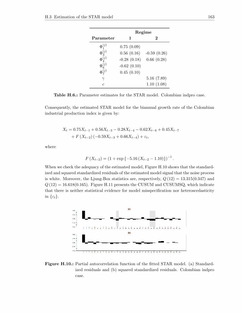
H.3 Estimation of the STAR model 163
Regime
Parameter 1 2
Φ(j)1 0.75 (0.09)
Φ(j)3 0.56 (0.16) -0.59 (0.26)
Φ(j)4 -0.28 (0.18) 0.66 (0.28)
Φ(j)6 -0.62 (0.10)
Φ(j)7 0.45 (0.10)
γ 5.16 (7.89)
c 1.10 (1.08)
Table H.6.: Parameter estimates for the STAR model. Colombian indpro case.
Consequently, the estimated STAR model for the biannual growth rate of the Colombian
industrial production index is given by:
Xt = 0.75Xt−1 + 0.56Xt−3 − 0.28Xt−4 − 0.62Xt−6 + 0.45Xt−7
+ F (Xt−2) (−0.59Xt−3 + 0.66Xt−4) + εt,
where
F (Xt−2) = (1 + exp {−5.16 (Xt−2 − 1.10)})−1 .
When we check the adequacy of the estimated model, Figure H.10 shows that the standard-
ized and squared standardized residuals of the estimated model signal that the noise process
is white. Moreover, the Ljung-Box statistics are, respectively, Q (12) = 13.315(0.347) and
Q (12) = 16.618(0.165). Figure H.11 presents the CUSUM and CUSUMSQ, which indicate
that there is neither statistical evidence for model misspecification nor heteroscedasticity
in {εt}.
Figure H.10.: Partial autocorrelation function of the fitted STAR model. (a) Standard-
ized residuals and (b) squared standardized residuals. Colombian indpro
case.

H.4 Estimation of the MSAR model 164
Figure H.11.: (a) CUSUM and (b) CUSUMSQ charts for the residuals of the fitted STAR
model. Colombian indpro case.
H.4. Estimation of the MSAR model
Table H.7 shows the estimates of the parameters of the model and their respective standard
errors in parenthesis.
state
Parameter 1 2
Φ(j)0 -0.24 (0.28) 0.89 (0.42)
Φ(j)1 0.31 (0.10) 0.80 (0.19)
Φ(j)2 0.70 (0.10) -0.12 (0.22)
Table H.7.: Parameter estimates for the MSAR model. Colombian indpro case.
Therefore, the estimated MSAR model for the biannual growth rate of the Colombian
industrial production index is given by:
Xt =
{−0.24 + 0.31Xt−1 + 0.70Xt−2 + ε1t, if st = 1
0.89 + 0.80Xt−1 − 0.12Xt−2 + ε2t, if st = 2
The conditional mean of Xt for regime 1 is -0.35 and for regime 2 is 4.52. The sample
variances of ε1t and ε2t are 1.62 and 5.75, respectively63. Hence, the first state could rep-
resent an unstable economy with decreases in the growth rate of the industrial production
index in average, and the second state could represent a stable economy with increases in
the growth rate of this macroeconomic indicator in average.
When we evaluate this model, Figure H.12 shows that the standardized and squared stan-
dardized residuals of the model signal that the noise process is white. Moreover, the
Ljung-Box statistics are, respectively, Q (12) = 4.767(0.965) and Q (12) = 2.065(0.999).
63 The probabilities of moving from one state to the other are p (st = 2|st−1 = 1) = 0.70(0.24) and
p (st = 1|st−1 = 2) = 0.60(0.25), where the number in parenthesis is the standard error. Addition-
ally, the unconditional probability that the process is in regime 1 is 0.46 and that it is in regime 2 is
0.54.

H.5 Estimation of the AR model 165
Figure H.13 presents the CUSUM and CUSUMSQ, which indicate that there is statistical
evidence for model misspecification and homoscedasticity in {εt}.
Figure H.12.: Partial autocorrelation function of the fitted MSAR model. (a) Standard-
ized residuals and (b) squared standardized residuals. Colombian indpro
case.
Figure H.13.: (a) CUSUM and (b) CUSUMSQ charts for the residuals of the fitted MSAR
model. Colombian indpro case.
H.5. Estimation of the AR model
We estimate an AR(2) model for the biannual growth rate of the Colombian industrial
production index64, which is given by:
(1− 0.52B − 0.34B2
)Xt = at, σ2a = 4.91.
The standard error of both coefficients is 0.09. When we check the residuals, Figure H.14
shows that the standardized residuals of the model slightly signal that some linear structure
in the data is not explained by the model, and the Ljung-Box statistics are, respectively,
Q (12) = 31.400(0.002) and Q (12) = 13.494(0.334). Figure H.15 shows the CUSUM and
64 As reported by the Phillips Perron (PP) (p − value = 0.002) and Kwiatkowski-Phillips-Schmidt-Shin
(KPSS) (Test statistic = 0.205 and Critical value = 0.463, the growth rate of the Colombian industrial
production index is stationary at the 5% significance level. The Augmented Dickey-Fuller (ADF) p −value is 0.143.

H.5 Estimation of the AR model 166
CUSUMSQ, indicating that there is no statistical evidence for model misspecification or
heteroscedasticity in {εt}.
Figure H.14.: Partial autocorrelation function of the fitted AR model. (a) Standardized
residuals and (b) squared standardized residuals. Colombian indpro case.
Figure H.15.: (a) CUSUM and (b) CUSUMSQ charts for the residuals of the fitted AR
model. Colombian indpro case.

Appendix I
General review of the models estimation for thegrowth rate of the Colombian CPI
I.1. Estimation of the TAR model
We use as the variable of interest, the growth rate of the Colombian CPI, and as the
threshold variable, we use the spread term mentioned above. Figure I.1 and Figure I.2
show that both series have significant autocorrelations for a large number of lags.
Figure I.1.: (a) Sample autocorrelation function and (b) sample partial autocorrelation
function for the growth rate of Colombian CPI.
I.1 Estimation of the TAR model 168
Figure I.2.: (a) Sample autocorrelation function and (b) sample partial autocorrelation
function for the Colombian spread term.
Then, we test the null hypothesis of AR linearity against the alternative of bivariate TAR
nonlinearity. Under the AIC criterion, we found that k = 3 is a reasonable autoregressive
order for Xt. Under the null hypothesis, the results of the test let us define as the delay
parameter of 3 for the threshold variable, thus, the input variable for the dynamic system
is Zt−3.
Figure I.3 shows the growth rate of the Colombian CPI and spread term from 2003:04 to
2012:06. The shading areas denote the business cycle contractions from peak to trough
based on Alfonso et al. (2012).
Figure I.3.: (a) Time plot of the growth rate of Colombian CPI and (b) Time plot of
Colombian spread term.
We specify the maximum number of regimes l0 by means of a regression function between
Xt and Zt, that is estimated using a nonparametric kernel approach and that is presented
in Figure I.4. We observe that 3 could be postulated as the possible maximum regimes for
the TAR model.
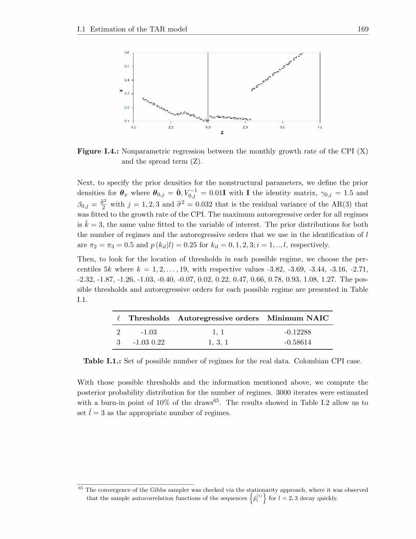
I.1 Estimation of the TAR model 169
Figure I.4.: Nonparametric regression between the monthly growth rate of the CPI (X)
and the spread term (Z).
Next, to specify the prior densities for the nonstructural parameters, we define the prior
densities for θx where θ0,j = 0, V −10,j = 0.01I with I the identity matrix, γ0,j = 1.5 and
β0,j = σ2
2 with j = 1, 2, 3 and σ2 = 0.032 that is the residual variance of the AR(3) that
was fitted to the growth rate of the CPI. The maximum autoregressive order for all regimes
is k = 3, the same value fitted to the variable of interest. The prior distributions for both
the number of regimes and the autoregressive orders that we use in the identification of l
are π2 = π3 = 0.5 and p (kil|l) = 0.25 for kil = 0, 1, 2, 3; i = 1, .., l, respectively.
Then, to look for the location of thresholds in each possible regime, we choose the per-
centiles 5k where k = 1, 2, . . . , 19, with respective values -3.82, -3.69, -3.44, -3.16, -2.71,
-2.32, -1.87, -1.26, -1.03, -0.40, -0.07, 0.02, 0.22, 0.47, 0.66, 0.78, 0.93, 1.08, 1.27. The pos-
sible thresholds and autoregressive orders for each possible regime are presented in Table
I.1.
` Thresholds Autoregressive orders Minimum NAIC
2 -1.03 1, 1 -0.12288
3 -1.03 0.22 1, 3, 1 -0.58614
Table I.1.: Set of possible number of regimes for the real data. Colombian CPI case.
With those possible thresholds and the information mentioned above, we compute the
posterior probability distribution for the number of regimes. 3000 iterates were estimated
with a burn-in point of 10% of the draws65. The results showed in Table I.2 allow us to
set l = 3 as the appropriate number of regimes.
65 The convergence of the Gibbs sampler was checked via the stationarity approach, where it was observed
that the sample autocorrelation functions of the sequences{p(i)l
}for l = 2, 3 decay quickly.

I.1 Estimation of the TAR model 170
` p`
2 0.2173
3 0.7827
Table I.2.: Posterior probability function for the number of regimes for the real data.
Colombian CPI case.
Thus, conditional on l = 3, we estimate the autoregressive orders for k1, k2 and k3. Based
on Table I.3, the identified autoregressive orders are k1 = 2, k2 = 1 and k3 = 2. As before,
convergence of the Gibbs sampler was checked via stationarity, and for 5000 iterates with a
burn-in point of 10% of the draws, it is observed that the sample autocorrelations functions
decay quickly66.
Regime
Autoregressive
Order1 2 3
0 0.0252 0.0047 7.54×10−06
1 0.2118 0.5358 0.2129
2 0.6848 0.0313 0.3954
3 0.0782 0.4282 0.3917
Table I.3.: Posterior probabilities for the autoregressive orders in the real data. Colom-
bian CPI case.
Consequently, we fit a TAR(3;2,1,2) with thresholds values r1 = −1.03 and r2 = 0.22,
which respectively are the 45th and 65th percentiles of the spread term. Table I.4 shows
the estimates for the nonstructural parameters, with their respective posterior standard
error in parenthesis and 90% credible interval in brackets67. These results show that not all
the coefficients are significant at the 5% level. However, we decide to estimate the model
with all the coefficients, given that that improves the final estimation.
66 We performed a sensibility analysis where we changed the prior densities of the autoregressive orders
and the nonstructural parameters, and it was found that the estimated autoregressive orders are the
same for different priors of the nonstructural parameters and for different priors of the autoregressive
orders.67 5000 iterates were generated with a burn-in point of 10% of the draws, and it was found that the
autocorrelation functions for all the parameters decay quickly, indicating the convergence of the Gibbs
sampler.

I.1 Estimation of the TAR model 171
Regime
Parameter 1 2 3
a(j)0
0.11 (0.04)
[0.04, 0.18]
0.16 (0.03)
[0.10, 0.21]
0.01 (0.03)
[−0.04, 0.07]
a(j)1
0.22 (0.15)
[−0.03, 0.47]
0.32 (0.11)
[0.14, 0.50]
0.69 (0.17)
[0.40, 0.97]
a(j)2
0.12 (0.15)
[−0.13, 0.37]
0.15 (0.20)
[−0.18, 0.48]
h(j)0.04 (0.01)
[0.03, 0.05]
0.01 (0.00)
[0.01, 0.02]
0.03 (0.01)
[0.02, 0.05]
Table I.4.: Parameter estimates for the TAR model. Colombian CPI case.
The fitted TAR model for the growth rate of the Colombian CPI is given by:
Xt =
0.11 + 0.22Xt−1 + 0.12Xt−2 + 0.04εt, if Zt−3 ≤ −1.03
0.16 + 0.32Xt−1 + 0.01εt, if −1.03 < Zt−3 ≤ 0.22
0.01 + 0.69Xt−1 + 0.15Xt−2 + 0.03εt, if Zt−3 > 0.22
This model could represent i) a first regime characterized by negative spreads, that respond
to contractionary monetary policies, and generate a slowdown real activity with minor
fluctuations in the inflation; ii) a second regime with an economic transition with a stable
behavior of the inflation; and iii) a third regime with positive spreads, that respond to
expansionary monetary policies, and produce real activity increases associated with major
fluctuations in the inflation.
When we check the residuals, in Figure I.5 we observe that the standardized and squared
standardized residuals signal that some nonlinear structure in the data is not explained
by the model. The Ljung-Box statistics are, respectively, Q (12) = 34.736(0.001) and
Q (12) = 8.216(0.768). Figure I.6 shows the CUSUM and CUSUMSQ, that indicate that
there is no statistical evidence for model misspecification but there is heteroscedasticity in
{εt}.
Figure I.5.: Partial autocorrelation function of the fitted TAR model. (a) Standardized
residuals and (b) squared standardized residuals. Colombian CPI case.

I.2 Estimation of the SETAR model 172
Figure I.6.: (a) CUSUM and (b) CUSUMSQ charts for the residuals of the fitted TAR
model. Colombian CPI case.
I.2. Estimation of the SETAR model
Based on the autocorrelation functions in Figure I.1 and the AIC and BIC criterion, we
identify p=3 as the final autoregressive order to fit a SETAR model. Once we select the
autoregressive model, we check the nonlinearity of the series based on Tsay’s (1989) test
and find that with d = 3, it is obtained the p-value = 0.0578 of the F statistic F = 2.577,
rejecting the linearity of the series at the 10% significance level.
Figure I.7 shows the sequence of the t ratios of a lag-3 AR coefficient versus the threshold
variable Xt−d in an arranged autoregression of order 3, and we identify that the data can
be divided into two regimes with a possible threshold at Xt−d = 0.09, because of the change
on the slope at approximately this point.
Figure I.7.: Time plot of t-ratio of recursive estimates of the AR-3 coefficient in an ar-
ranged autoregression of order 3 and delay parameter 3. Colombian CPI
case.
We also use the NAIC criterion of Tong (1990), which suggests a threshold value of rj = 0.07
and autoregressive orders AR(2) and AR(1) for each regime, with a NAIC = -370.198.
Based on that, we fit a SETAR(2;2,1) for the monthly growth rate of the CPI, with
threshold value Xt−3. The estimated parameters and their standard errors in parenthesis
for each regime are shown in Table I.5, where all estimates are significant at the 5% level.

I.2 Estimation of the SETAR model 173
Regime
Parameter 1 2
Φ(j)0 0.08 (0.03)
Φ(j)1 0.54 (0.16) 0.46 (0.11)
Φ(j)2 0.34 (0.17)
Table I.5.: Parameter estimates for the SETAR model. Colombian CPI case.
In that sense, the fitted SETAR model for the growth rate of the Colombian CPI is given
by:
Xt =
{0.54Xt−1 + 0.34Xt−2 + εt, if Xt−3 ≤ 0.07
0.08 + 0.46Xt−1 + εt, if Xt−3 > 0.07
This model could represent i) a first regime characterized by a real activity tightening
associated with minor fluctuations in the inflation; and ii) a second regime with a real
activity increasing associated with major fluctuations in the inflation.
Figure I.8 shows that the correlations of the standardized and squared standardized resid-
uals of the model could signal that the noise process is white, and the Ljung-Box statistics
are, respectively, Q (12) = 17.405(0.135) and Q (12) = 7.777(0.802). Figure I.9 presents
the CUSUM and CUSUMSQ, indicating that there is no statistical evidence for model
misspecification and there is some heteroscedasticity in {εt}.
Figure I.8.: Partial autocorrelation function of the fitted SETAR model. (a) Standardized
residuals and (b) squared standardized residuals. Colombian CPI case.

I.3 Estimation of the STAR model 174
Figure I.9.: (a) CUSUM and (b) CUSUMSQ charts for the residuals of the fitted SETAR
model. Colombian CPI case.
I.3. Estimation of the STAR model
With an identified p = 2 autoregressive order, we evaluate the nonlinearity of the series
based on Terasvirta’s test and find that, with a delay parameter of d = 1, we obtain the
p-value = 0.0648 for the F statistic F = 2.0589, which rejects the linearity of the time
series.
When we compute the tests of nested hypothesis of Terasvirta (1994), we find that at the
5% significance level, H01 and H02 are not rejected, while H03 is not, where the respective
p-value is 0.7155, 0.4696 and 0.0072. These results suggest that we must estimate a LSTAR
model.
In Table I.6, we show the estimates for the parameters and their respective standard error
in parenthesis, where only the lag-4 AR coefficient of the first regime and the parameter γ
and c are not significant at the 5% level.
Regime
Parameter 1 2
Φ(j)1 -0.29 (0.33) 0.93 (0.35)
Φ(j)2 0.11 (0.10)
γ 5.08 (10.84)
c -0.14 (0.10)
Table I.6.: Parameter estimates for the STAR model. Colombian CPI case.
Consequently, the fitted STAR model for the growth rate of the Colombian CPI is given
by:
Xt = −0.29Xt−1 + 0.11Xt−2 + F (Xt−1) (0.93Xt−1) + εt,
where
F (Xt−1) = (1 + exp {−5.08 (Xt−1 + 0.14)})−1 .

I.4 Estimation of the MSAR model 175
When we check the residuals, Figure I.10 shows that the standardized and squared stan-
dardized residuals of the model could signal that the noise process is white. Further-
more, the Ljung-Box statistics are, respectively, Q (12) = 17.640(0.127) and Q (12) =
11.140(0.517). Figure I.11 presents the CUSUM and CUSUMSQ, which indicate that
there is no statistical evidence for model misspecification but there is heteroscedasticity in
{εt}.
Figure I.10.: Partial autocorrelation function of the fitted STAR model. (a) Standardized
residuals and (b) squared standardized residuals. Colombian CPI case.
Figure I.11.: (a) CUSUM and (b) CUSUMSQ charts for the residuals of the fitted STAR
model. Colombian CPI case.
I.4. Estimation of the MSAR model
Table I.7 shows the estimates of the parameters of the model and their respective standard
errors in parenthesis.

I.4 Estimation of the MSAR model 176
state
Parameter 1 2
Φ(j)0 0.02 (0.02) 0.11 (0.04)
Φ(j)1 0.43 (0.15) 0.39 (0.15)
Φ(j)2 0.10 (0.13) 0.20 (0.17)
Table I.7.: Parameter estimates for the MSAR model. Colombian CPI case.
Therefore, the fitted MSAR model for the monthly growth rate of the Colombian CPI is
given by:
Xt =
{0.02 + 0.43Xt−1 + 0.10Xt−2 + ε1t, if st = 1
0.11 + 0.39Xt−1 + 0.20Xt−2 + ε2t, if st = 2
The conditional mean of Xt for regime 1 is 0.04 and for regime 2 is 0.18 The sample
variances of ε1t and ε2t are 0.01 and 0.05, respectively68. Hence, the first state could
represent a minor stable economy with minor fluctuations in the CPI, and the second state
could represent a stable economy with increases in the CPI.
When we check the residuals, Figure I.12 shows that the standardized and squared stan-
dardized residuals of the model signal that the noise process is white, and the Ljung-Box
statistics are, respectively, Q (12) = 11.220(0.510) and Q (12) = 0.865(0.999). Figure I.13
presents the CUSUM and CUSUMSQ, which indicates that there is statistical evidence for
some model misspecification and heteroscedasticity in {εt}.
Figure I.12.: Partial autocorrelation function of the fitted MSAR model. (a) Standard-
ized residuals and (b) squared standardized residuals. Colombian CPI case.
68 The probabilities of moving from one state to the other are p (st = 2|st−1 = 1) = 0.18(0.10) and
p (st = 1|st−1 = 2) = 0.78(0.14), where the number in parenthesis is the standard error. Addition-
ally, the unconditional probability that the process is in regime 1 is 0.55 and that it is in regime 2 is
0.45.
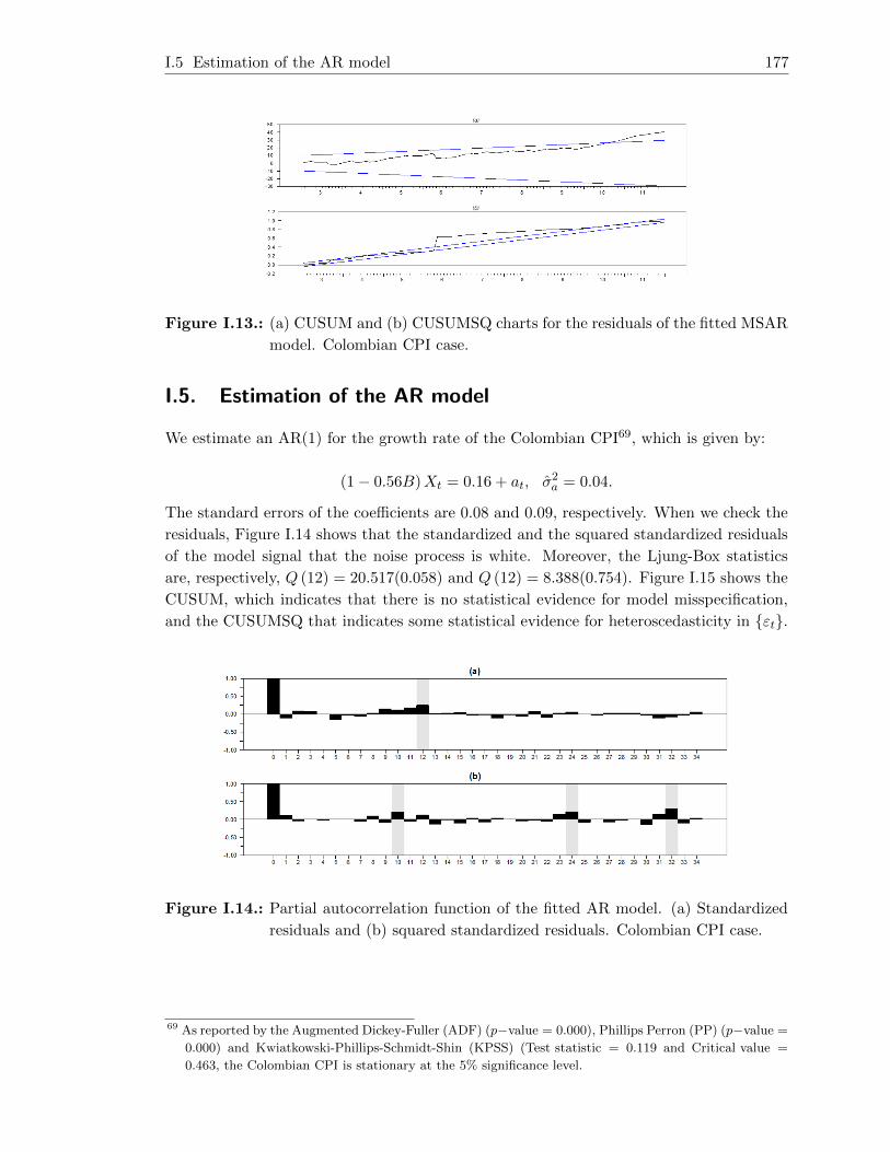
I.5 Estimation of the AR model 177
Figure I.13.: (a) CUSUM and (b) CUSUMSQ charts for the residuals of the fitted MSAR
model. Colombian CPI case.
I.5. Estimation of the AR model
We estimate an AR(1) for the growth rate of the Colombian CPI69, which is given by:
(1− 0.56B)Xt = 0.16 + at, σ2a = 0.04.
The standard errors of the coefficients are 0.08 and 0.09, respectively. When we check the
residuals, Figure I.14 shows that the standardized and the squared standardized residuals
of the model signal that the noise process is white. Moreover, the Ljung-Box statistics
are, respectively, Q (12) = 20.517(0.058) and Q (12) = 8.388(0.754). Figure I.15 shows the
CUSUM, which indicates that there is no statistical evidence for model misspecification,
and the CUSUMSQ that indicates some statistical evidence for heteroscedasticity in {εt}.
Figure I.14.: Partial autocorrelation function of the fitted AR model. (a) Standardized
residuals and (b) squared standardized residuals. Colombian CPI case.
69 As reported by the Augmented Dickey-Fuller (ADF) (p−value = 0.000), Phillips Perron (PP) (p−value =
0.000) and Kwiatkowski-Phillips-Schmidt-Shin (KPSS) (Test statistic = 0.119 and Critical value =
0.463, the Colombian CPI is stationary at the 5% significance level.

I.5 Estimation of the AR model 178
Figure I.15.: (a) CUSUM and (b) CUSUMSQ charts for the residuals of the fitted AR
model. Colombian CPI case.

Bibliography
Alfonso, V., Arango, L., Arias, F., and Pulido, J. (2012). Ciclos de negocios en colombia:
1975-2011. Borradores de Economıa, (651): 1–23.
Arango, L. and Florez, L. (2004). Expectativas de actividad economica en colombia y
estructura a plazo: un poco mas de evidencia. Revista ESPE, (47): 126–160.
Arango, L., Florez, L., and Arosemena, A. (2004). El tramo corto de la estructura a plazo
como predictor de expectativas de la actividad economica en colombia. Borradores de
Economıa, (279): 1–21.
Avella, R. (2001). Efecto de las sequıas sobre la inflacion en colombia. Borradores de
Economıa, (183): 1–55.
Banerjee, A. and Marcellino, M. (2006). Are there any reliable leading indicators for us
inflation and gdp growth? International Journal of Forecasting, 22 (1): 137– 151.
Bernanke, B. (1990). On the predictive power of interest rates and interest rate spreads.
New England Economic Review, (November/December): 51–68.
Bernanke, B. and Blinder, A. (1992). The federal funds rate and the channels of monetary
transmission. The American Economic Review, 82 (4): 901–921.
Black, D., Corrigan, P., and Dowd, M. (2000). New dogs and old tricks: do money
and interest rates still provide information content for forecasts of output and prices?
International Journal of Forecasting, 16 (2): 191–205.
Blanchard, O. and Johnson, D. (2013). Macroeconomics. Pearson Education, England, 6
edition.
Box, G., Jenkins, G., Reinsel, G., and Ljung, G. (2016). Time Series Analysis: Forecasting
and Control. John Wiley & Sons, New Jersey, 5 edition.
Bradley, M. and Jansen, D. (2004). Forecasting with a nonlinear dynamic model of stock
returns and industrial production. International Journal of Forecasting, 20 (2): 321–342.
Bry, G. and Boschan, C. (1971). Cyclical Analysis of Time Series: Selected Procedures and
Computer Programs. NBER, New York.
Bibliography 180
Calderon, S. (2014). Bayesian Analysis of Multivariate Threshold Autoregressive Models
with Missing Data. Doctoral thesis, Universidad Nacional de Colombia, Bogota, Colom-
bia.
Cao, C. and Tsay, R. (1992). Nonlinear time-series analysis of stock volatilities. Journal
of Applied Econometrics, 7 (11): S165–S185.
Casella, G. and George, E. (1992). Explaining the gibbs sampler. The American Statisti-
cian, 46 (3): 167–174.
Cecchetti, S., Chu, R., and Steindel, C. (2000). The unreliability of inflation indicators.
Current Issues in Economics and Finance, 6 (4): 1–6.
Chan, K. and Tong, H. (1986). On estimating thresholds in autoregressive models. Journal
of Time Series Analysis, 7 (3): 179–190.
Chong, Y. and Hendry, D. (1986). Econometric evaluation of linear macro-economic mod-
els. Review of Economic Studies, 53 (4): 671–690.
Clements, M. (2005). Evaluating Econometric Forecasts of Economic and Financial Vari-
ables. Palgrave Macmillan, New York.
Clements, M., Franses, P., Smith, J., and van Dijk, D. (2003). On setar non-linearity and
forecasting. Journal of Forecasting, 22 (5): 359–375.
Clements, M. and Hendry, D. (1996). Intercept corrections and structural change. Journal
of Applied Econometrics, 11 (5): 475–494.
Clements, M. and Hendry, D. (1998). Forecasting economic time series. Cambridge Uni-
versity Press, Cambridge.
Clements, M. and Hendry, D. (2002). A companion to economic forecasting. Blackwell
Publishing, Malden.
Clements, M. and Krolzig, H. (1998). A comparison of the forecast performance of markov-
switching and threshold autoregressive models of us gnp. The Econometrics Journal,
1 (1): 47–75.
Clements, M. and Smith, J. (1999). A monte carlo study of the forecasting performance
of empirical setar models. Journal of Applied Econometrics, 14 (2): 123–141.
Clements, M. and Smith, J. (2000). Evaluating the forecast densities of linear and non-
linear models: applications to output growth and unemployment. Journal of Forecasting,
19 (4): 255–276.
Deschamps, P. (2008). Comparing smooth transition and markov switching autoregressive
models of us unemployment. Journal of Applied Econometrics, 23 (4): 435–462.
Diebold, F. and Mariano, R. (1995). Comparing predictive accuracy. Journal of Business
& Economic Statistics, 13 (3): 253–263.

Bibliography 181
Elger, T., Jones, B., and Nilsson, B. (2006). Forecasting with monetary aggregates: Recent
evidence for the united states. Journal of Economics and Business, 58 (5-6): 428–446.
Ericsson, N. (1992). Parameter constancy, mean squared forecast errors, and measuring
forecast performance: An exposition, extensions, and illustration. Journal of Policy
Modeling, 14 (4): 465–495.
Estrella, A. and Hardouvelis, G. (1991). The term structure as a predictor of real economic
activity. Journal of Finance, 46 (2): 555–576.
Estrella, A. and Mishkin, F. (1997). The predictive power of the real term structure of
interest rates in europe and the united states: Implications for the european central
bank. European Economic Review, 41 (7): 1375–1401.
Estrella, A. and Trubin, M. (2006). The yield curve as a leading indicator: Some practical
issues. Current Issues in Economics and Finance, 12 (5): 1–7.
Fama, E. (1990). Term structure forecasts of interest rates, inflation and real returns.
Journal of Monetary Economics, 25 (1): 59–76.
Franses, P. and van Dijk, D. (2000). Nonlinear time series models in empirical finance.
Cambridge University Press, Cambridge.
Franses, P. and van Dijk, D. (2005). The forecasting performance of various models for
seasonality and nonlinearity for quarterly industrial production. International Journal
of Forecasting, 21 (1): 87–102.
Friedman, B. and Kuttner, K. (1992). Money, income, prices, and interest rates. The
American Economic Review, 82 (3): 472–492.
Garzon, L. and Tobos, J. (2014). Efectos de los mercados crediticio y cambiario sobre
el crecimiento economico: el caso colombiano. Master’s thesis, Pontificia Universidad
Javeriana, Bogota, Colombia.
Gelman, A., Carlin, J., Stern, H., and Rubin, D. (2009). Bayesian Data Analysis. Chapman
and Hall/CRC, Boca Raton, 2 edition.
Geweke, J. and Amisano, G. (2010). Comparing and evaluating bayesian predictive distri-
butions of asset returns. International Journal of Forecasting, 26 (2): 216–230.
Geweke, J. and Terui, A. (1993). Bayesian threshold autoregressive models. Journal of
time series analysis, 14 (5): 441–454.
Gooijer, J. and Hyndman, R. (2006). 25 years of time series forecasting. International
Journal of Forecasting, 22 (3): 443–473.
Granger, C. (1993). Strategies for modelling nonlinear time-series relationships. Economic
Record, 69 (3): 233–238.
Granger, C. and Newbold, P. (1973). Some comments on the evaluation of economic
forecasts. Applied Economics, 5 (1): 35–47.

Bibliography 182
Granger, C. and Newbold, P. (1986). Forecasting Economic Time Series. Academic Press,
London, 2 edition.
Guidolin, M., Hyde, S., McMillan, D., and Ono, S. (2009). Non-linear predictability in
stock and bond returns: When and where is it exploitable? International Journal of
Forecasting, 25 (2): 373–399.
Guzman, O., Herrera, J., and Saenz, J. (2003). Contracciones leves y profundas: Efectos
asimetricos sobre la pobreza. el caso colombiano: 1984 – 2000. Archivos de Economıa,
(231): 1–44.
Hamilton, J. (1989). A new approach to the economic analysis of nonstationary time series
and the business cycle. Econometrica, 57 (2): 357–384.
Hamilton, J. (1993). Estimation, inference and forecasting of time series subject to changes
in regime. Handbook of Statistics, 11 : 231–260.
Hamilton, J. (1994). Time series analysis. Princeton University Press, Princeton.
Hansson, J., Jansson, P., and Lof, M. (2005). Business survey data: Do they help in
forecasting gdp growth? International Journal of Forecasting, 21 (2): 377–389.
Harding, D. and Pagan, A. (2002). Dissecting the cycle: a methodological investigation.
Journal of Monetary Economics, 49 (2): 365–381.
Harris, R. and Sollis, R. (2003). Applied time series modelling and forecasting. Wiley,
Chichester, 2 edition.
Harvey, C. (1988). The real term structure and consumption growth. Journal of Financial
Economics, 22 (2): 305–33.
Harvey, C. (1989). Forecasts of economic growth from the bond and stock markets. Fi-
nancial Analysts Journal, 45 (5): 38–45.
Harvey, C. (1997). The relation between the term structure of interest rates and canadian
economy growth. Canadian Journal of Economics, 30 (1): 169–193.
Harvey, D., Leybourne, S., and Newbold, P. (1997). Testing the equality of prediction
mean squared errors. International Journal of Forecasting, 13 (2): 281–291.
Harvey, D., Leybourne, S., and Newbold, P. (1998). Tests for forecast encompassing.
Journal of Business and Economic Statistics, 16 (2): 254–259.
Hoff, P. (2009). First course in Bayesian Statistical Methods. Springer, New York.
Holden, K. and Peel, D. (1989). Unbiasedness, efficiency and the combination of economic
forecast. Journal of Forecasting, 8 (3): 175–188.
Hoyos, N. (2006). Una aplicacion del modelo no lineal tar en economıa. Master’s thesis,
Universidad Nacional de Colombia, Bogota, Colombia.

Bibliography 183
Hyndman, R. (1995). Highest-density forecast regions for nonlinear and non-normal time
series models. Journal of Forecasting, 14 (5): 431–441.
Jorion, P. and Mishkin, F. (1991). A multicountry comparison of term-structure forecasts
at long horizons. Journal of Financial Economics, 29 (1): 59–80.
Keynes, J. (1936). The General Theory of Employment, Interest and Money. Harcourt,
New York.
Kolly, J. (2014). Predicting the US unemployment rate using Bayesian model averaging.
Doctoral thesis, University of Fribourg, Fribourg, Switzerland.
Koop, G. and Potter, S. (1999). Dynamic asymmetries in us unemployment. Journal of
Business and Economic Statistics, 17 (3): 298–312.
Kozicki, S. (1998). Predicting inflation with the term structure spread. Federal Reserve
Bank of Kansas City Research, Working Paper, (98-02): 1–39.
Kuosmanen, P. and Vataja, J. (2014). Forecasting gdp growth with financial market data
in finland: Revisiting stylized facts in a small open economy during the financial crisis.
Review of Financial Economics, 23 (2): 90–97.
Laurent, R. (1988). An interest rate-based indicator of monetary policy. Economic Per-
spectives, 12 (1): 3–14.
Manzan, S. and Zerom, D. (2013). Are macroeconomic variables useful for forecasting the
distribution of u.s. inflation? International Journal of Forecasting, 29 (3): 469–478.
Melo, L., Loaiza, R., and Villamizar, M. (2016). Bayesian combination for inflation fore-
casts: The effects of aprior based on central banks’ estimates. Economic Systems, 40 (3):
387–397.
Melo, L. and Nunez, H. (2004). Combinacion de pronosticos de la inflacion en presencia
de cambios estructurales. Borradores de Economıa, (286): 1–51.
Meyn, S. and R., T. (2009). Markov Chains and Stochastic Stability. Cambridge University
Press, Cambridge, 2 edition.
Mishkin, F. (1990). The information in the longer-maturity term structure about future
inflation. Quarterly Journal of Economics, 105 (3): 815–28.
Mishkin, F. (1991). A multi-country study of the information in the term structure about
future inflation. Journal of International Money and Finance, 10 (1): 2–22.
Montgomery, A., Zarnowitz, V., Tsay, R., and Tiao, G. (1998). Forecasting the u.s. unem-
ployment rate. Journal of the American Statistical Association, 93 (442): 478–493.
Nieto, F. (2005). Modeling bivariate threshold autoregressive processes in the presence of
missing data. Communications in Statistics-Theory and Methods, 34 (4): 905–930.
Nieto, F. (2008). Forecasting with univariate tar models. Statistical Methodology, 5 (3):
263–276.
Bibliography 184
Nieto, F. and Hoyos, M. (2011). Testing linearity against a univariate tar specification in
time series with missing data. Revista Colombiana de Estadıstica, 34 (1): 73–94.
Nieto, F. and Moreno, E. (2016). On the univariate conditional distributions of an open-
loop tar stochastic process. Revista Colombiana de Estadıstica, 39 (2): 149–165.
Nieto, F., Zhang, H., and Li, W. (2013). Using the reversible jump mcmc procedure
for identifying and estimating univariate tar models. Communications in Statistics:
Simulation and Computation, (42): 814–840.
Nunez, H. (2005). Una evaluacion de los pronosticos de inflacion en colombia bajo el
esquema de “inflacion objetivo. Revista de Economıa del Rosario, 8 (2): 151–185.
Rossi, B. and Sekhposyan, T. (2010). Have economic models’ forecasting performance for
us output growth and inflation changed over time, and when? International Journal of
Forecasting, 26 (4): 808–835.
Rossi, B. and Sekhposyan, T. (2014). Evaluating predictive densities of us output growth
and inflation in a large macroeconomic data set. International Journal of Forecasting,
30 (3): 662–682.
Rothman, P. (1998). Forecasting asymmetric unemployment rates. Review of Economics
and Statistics, 80 (1): 164–168.
Schuh, S. (2001). An evaluation of recent macroeconomic forecast errors. New England
Economic Review, (January/February): 35–56.
Stock, J. and Watson, M. (1989). Interpreting the evidence on money-income causality.
Journal of Econometrics, 40 (1): 161–181.
Stock, J. and Watson, M. (1999). Forecasting inflation. Journal of Monetary Economics,
44 (2): 293–335.
Stock, J. and Watson, M. (2003). Forecasting output and inflation: The role of asset prices.
Journal of Economic Literature, 41 (3): 788–829.
Terasvirta, T. (1994). Specification, estimation, and evaluation of smooth transition au-
toregressive models. Journal of the American Statistical Association, 89 (425): 208–218.
Terasvirta, T. (2006). Forecasting economic variables with nonlinear models. In Elliott, G.,
Granger, C., and Timmermann, A., editors, Handbook of Economic Forecasting, volume
1, pages 413–457, Amsterdam. Elsevier, North-Holland.
Terasvirta, T. and Anderson, H. (1992). Characterizing nonlinearities in business cycles
using smooth transition autoregressive models. Journal of Applied Econometrics, 7 (S1):
S119–S136.
Terasvirta, T., Tjøstheim, D., and Granger, C. (2010). Modelling nonlinear economic time
series. Oxford University Press, Oxford.
Theil, H. (1966). Applied Economic Forecasting. North Holland, Amsterdam.

Bibliography 185
Thoma, M. and Gray, J. (1998). Financial market variables do not predict real activity.
Economic Inquiry, 36 (4): 522–539.
Tiao, G. and Tsay, R. (1994). Some advances in non-linear and adaptive modeling in time
series. Journal of Forecasting, 13 (2): 109–131.
Tong, H. (1978). On a threshold model. In Chen, C., editor, Pattern recognition and signal
processing, pages 575–586, Amsterdam. Sijhoff & Noordhoff.
Tong, H. (1983). Threshold models in non-linear time series analysis. Springer-Verlag,
New York.
Tong, H. (1990). Non-Linear Time Series: A Dynamical Systems Approach. Oxford
University Press, Oxford.
Tong, H. and Lim, K. (1980). Threshold autoregressions, limit cycles, and cyclical data.
Journal of the Royal Statistical Society. Series B (methodological), 42 (3): 245–292.
Tsay, R. (1989). Testing and modeling threshold autoregressive processes. Journal of the
American Statistical Association, 84 (405): 231–240.
Tsay, R. (1998). Testing and modeling multivariate threshold models. Journal of the
American Statistical Association, 93 (443): 1188–1202.
Tsay, R. (2000). Time series and forecasting: Brief history and future research. Journal
of the American Statistical Association, 95 (450): 638–643.
Tsay, R. (2005). Analysis of financial time series. John Wiley & Sons, New Jersey, 2
edition.
van Dijk, D. and Franses, P. (2003). Selecting a nonlinear time series model using weighted
tests of equal forecast accuracy. Oxford Bulletin of Economics and Statistics, 65 (S1):
727–744.
van Dijk, D., Terasvirta, T., and Franses, P. (2002). Smooth transition autoregressive
models. a survey of recent developments. Econometric Reviews, 21 (1): 1–47.
Vargas, L. (2012). Calculo de la distribucion predictiva en un modelo tar. Master’s thesis,
Universidad Nacional de Colombia, Bogota, Colombia.
Vivas, K. (2011). Modelacion no lineal de la tasa de desempleo urbano para colombia.
Master’s thesis, Universidad Nacional de Colombia, Bogota, Colombia.
Wheelock, D. and Wohar, M. (2009). Can the term spread predict output growth and
recessions? a survey of the literature. Federal Reserve Bank of St. Louis Review, 91 (5,
Part 1): 419–40.
Wong, C. and Li, W. (2000). On a mixture autoregressive model. Journal of the Royal
Statistical Society. Series B Statistical Methodology, 62 (1): 95–115.