analysis of the correlation between the price and volume in ...between the trading volume and the...

International Journal of Science and Research (IJSR) ISSN (Online): 2319-7064

Index Copernicus Value (2016): 79.57 | Impact Factor (2017): 7.296

Volume 7 Issue 6, June 2018

www.ijsr.net Licensed Under Creative Commons Attribution CC BY

Analysis of the Correlation between the Price and Volume in Shanghai Stock Market

Jinhan Zhao

Xidian University Economics and Management Institute, Shanxi Xi’an 710071, China

Abstract: The article applied least-squares estimation and quantile regression to study the relationship between the volume and closing

price in Shanghai stock market , turning to linear studies, which makes the correlation of stock trading volume and price for promotion,

and conclusions are drawn that is different from predecessors' . The empirical results show that there is a stable positive correlation

between the trading volume and the closing price of Shanghai stock market, that is, the higher the trading volume is, the higher the

closing price is, and the equation is significant. At the 70%, 75% and 80% quantile level of volume, the correlation between the two is

greatly Iimproved , and the performance is highly linear. The results show that when the stock is rising ,the high volume of the shares

can be judged as the high point of the stock price, which determines the selling probability and the corresponding upper limit of risk

value. This conclusion is helpful for investors to judge the trend of stock, reduce the losses caused by non-rational factors, and have the

guiding significance in the stock selling operation.

Keywords: The relation between volume and price; Linear regression; Volume; Stock price;

1. Introduction

The relationship between stock trading volume and stock

price (abbreviated as volume price relationship) has always

been the focus of investors when investigating stocks. In

this article, the Granger causality test results show that the

stock price of the Shanghai stock market is not subject to

random walk, but can use the historical information to

predict the future. Since the volume reflects all the factors

that affect the stock price change, the volume directly

affects the price of the stock. Finding the relationship

between stock turnover and price helps investors to

anticipate the future trend of the stock market.

Compared with previous literature, the innovation of this

paper is:

1) Changed the dependent variable of the quantity and price

relationship, making the stock price and trading volume

show a significant positive linear relationship, replacing

the previous non-linear relationship.

2) Using quantile regression, the coefficient of all the

quantiles of trading volume maintains a stable positive

correlation, which resolves the “ left tail” correlation

change of the seniors, that is, the negative correlation

between volume and price turns into a positive

correlation.

3) Under all trading volume points, the relationship

between trading volume and stock price is significant at

1%, which optimizes the situation where volume and

stock returns have nothing to do with certain points.

This article is devoted to the study of the correlation

between stock prices and trading volume, and through the

correlation, makes a corresponding judgment on the stock

price corresponding to the volume at each point, and uses

probabilistic thinking to predict its trend. To help investors

rationally judge the stock price, the probability distribution

of the stock price trend, and the corresponding maximum

risk situation, and to guide the probability of selling stock

operation, so that investors can obtain the best expected

return and reduce investment risk, and can be highly

efficient investment.

2. Literature Review

The research on the relationship between volume and price in foreign markets focuses on the relationship between volume and profitability. Saatcioglu K, Starks LT (1998) research shows that emerging markets that lead changes in stock prices have different institutional and information flows than developed markets, but do not show similar stock prices and research advantages using U.S. data gap. In a series of emerging markets, the differences in institutional and information flows are important enough to affect the valuation process of stocks

[1]. Chen S H, Liao C C (1999)

found that the agency-based approach is more fundamental to the interpretation of volume-price relations. The results show that the stock price relationship can be regarded as a general property of the financial market, and it believes that unless the feedback relationship between the individual behavior at the bottom and the agglomeration phenomenon at the top is well explained, the volume cannot be fully accepted. The relationship between yields

[2]. Ciner C (2002)

used structure and vector autoregressive models to study the information content of the trading volume of the Toronto Stock Exchange before and after a fully electronic transaction. The empirical results show that price discovery improved in electronic transactions will reduce the forecasting capacity of trading volume. After fully automated, the predictive power of price changes disappeared

[3]. Badhani KN (2006) studied the causality

between stock prices based on the total trading volume of the S&P CNX and the national stock exchange

[4]. Mahajan S,

Singh B (2008) used the daily data of the Bombay Stock Exchange Sensitivity Index to study the empirical relationship between the market structure hypothesis and the market structure. The study concluded that the volume provides information with precise and discrete information, rather than as information. The representative of the signal [5].

Paper ID: ART20183006 DOI: 10.21275/ART20183006 201

www.ijsr.net

http://creativecommons.org/licenses/by/4.0/





Many scholars began to study the relationship between

trading volume and profitability in the Chinese stock market

on the basis of Western research on quantity and price.

Wang CW (2002) examined the linear and nonlinear

Granger causality between the trading volume and price in

the Shanghai and Shenzhen stock markets. The results show

that there is a linear Granger causality and two-way

non-reversion from stock returns to trading volume. Linear

Granger causality, but after filtering the weekend and

GARCH effects, the nonlinear Granger causality

disappeared [6]

. Wei Y U, Yin J (2006) found that there is a

long-term equilibrium between price and volume, and price

changes can explain changes in volume, but it is not entirely

correct [7]

. Qian Zhengming (2007) studied the quantile

regression analysis of the relationship between volume and

price in the Shanghai stock exchange market [8]

. Zheng T T,

Zhang C C, Xing W (2009) studied that price rules are not

consistent in different stocks [9]

. Lu Ying, Liu Xiaoyan (2015) discusses the correlation between stock returns and trading

volume [10]

. Ren Yanyan, Li Wei, RENYan-yan, et al (2017) compared the quantile regression (QR) model with the

IVQR model and analyzed the relationship between the

return rate and the volume under different quintiles [11]

.

The previous generation did not draw a stable and

persuasive result on the relationship between the stock price

and the stock price in terms of stock returns and trading

volume. The conclusion only showed some basic

characteristics between the quantity and price. The

persuasive power was insufficient and it was necessary to

The research of the relationship is improved and

transformed. Among them, Ding D K, Lau S T (2001) studied the relationship between the absolute price of two

kinds of crude oil and trading volume and the results

showed a high degree of consistency [12]

. Smirlock M,

Starks L (2015) studied volume and absolute prices. The

results show that at the company level, there is a significant

causal relationship between volume and price, and this

relationship is stronger in related earnings announcements [13]

. Chen Langnan, Luo Jiawen, and Liu Xin (2015) illustrate the time-varying shock response to price structure

and trading volume changes in market structure and the

time-varying shock effect of short-selling trading

mechanism[14]

. However, the focus of this paper is that

changes in stock prices change over time. There is no

specific situation where the relationship between volume

and price is positively related.

However, there are few researches on the relationship

between the absolute stock price and the trading volume,

and the specific situation of the quantity-price relationship is

worth further studying and excavating the value of its

practical application. Therefore, it can be considered to

apply it to the Shanghai stock market, relying on the high

significance of absolute prices and trading volume to study

the correlation between absolute stock price and trading

volume of the Shanghai stock market.

3. Basic ideas of the model

3.1 Least squares estimation

The problem of estimating certain parameters through one

or more sets of observations is common in actual production.

For example, the stock price of a stock that rises at a

constant rate at time t is Y, which can be described by the

following linear function (1):

ˆ tay (1)

Where a is the initial price of the stock price at t =0, and

is the average growth rate of the stock price. Since

observations in the actual process cannot be very accurate

and the observations have accidental errors, we need to

make redundant observations of the observations to exclude

their randomness. At this time, in order to obtain the

estimated values a and , it is necessary to separately

measure the position at different time points t1，t2，t3，...tn

to obtain a set of observation values y1，y2，y3，...yn. At this

time, from the above formula (1) can be obtained (2)

),,2,1(,ˆˆ niytv iii

(2)

If

n

t

t

t

y

y

y

v

v

v

VXBY

n

n

n

n

n ...ˆ

2

1

,ˆ

ˆ,

...

1

...

1

1

,...

1,

1,2

2

1

2,

2

1

1,

Then formula (2) is:

YXBV ˆ (3)

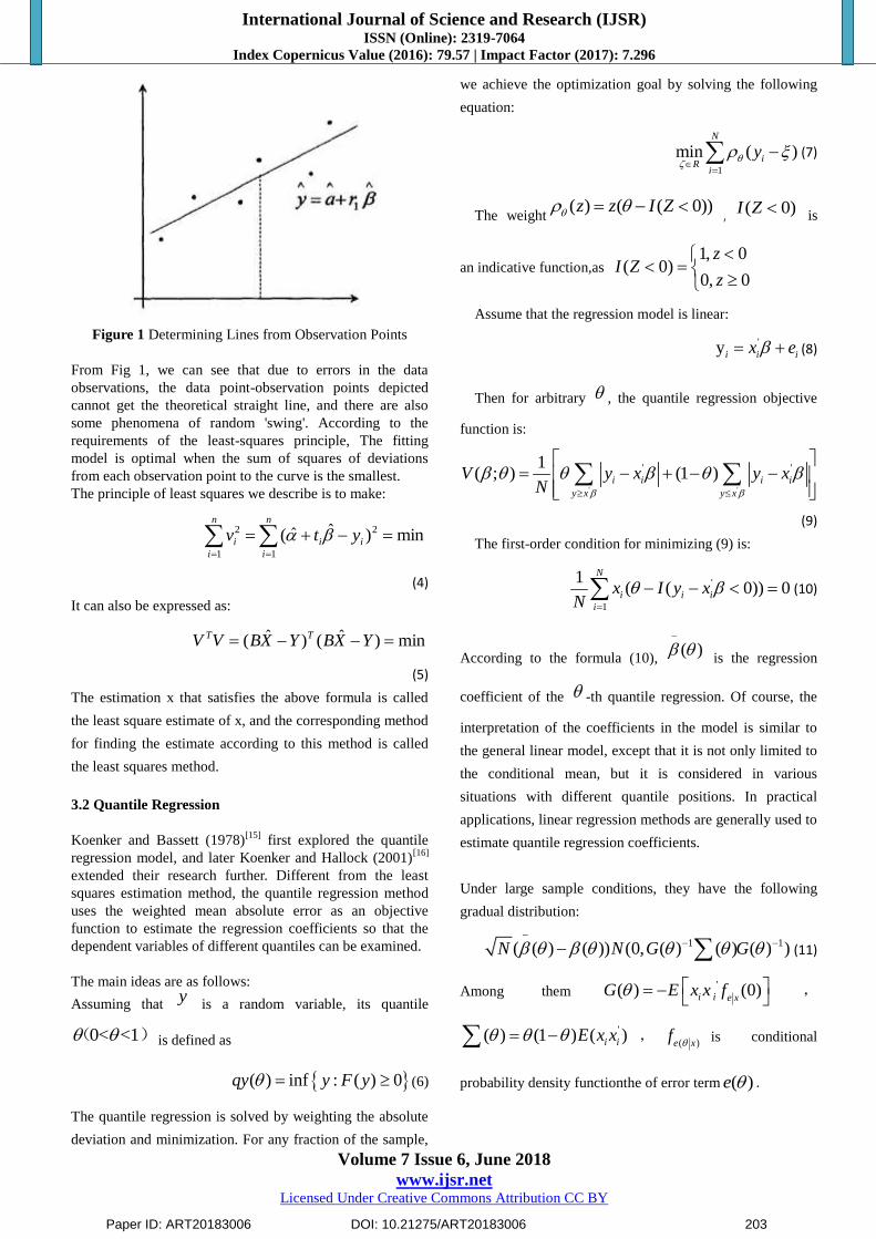
Corresponding yi, ti (i =1, 2, ...n) is illustrated in Figure 1

below.


www.ijsr.net






Figure 1 Determining Lines from Observation Points

From Fig 1, we can see that due to errors in the data

observations, the data point-observation points depicted

cannot get the theoretical straight line, and there are also

some phenomena of random 'swing'. According to the

requirements of the least-squares principle, The fitting

model is optimal when the sum of squares of deviations

from each observation point to the curve is the smallest.

The principle of least squares we describe is to make:

n

i

n

i

iii ytv1 1

22 min)ˆˆ(

(4)

It can also be expressed as:

min)ˆ()ˆ( YXBYXBVV TT

(5)

The estimation x that satisfies the above formula is called

the least square estimate of x, and the corresponding method

for finding the estimate according to this method is called

the least squares method.

3.2 Quantile Regression

Koenker and Bassett (1978)[15]

first explored the quantile

regression model, and later Koenker and Hallock (2001)[16]

extended their research further. Different from the least

squares estimation method, the quantile regression method

uses the weighted mean absolute error as an objective

function to estimate the regression coefficients so that the

dependent variables of different quantiles can be examined.

The main ideas are as follows:

Assuming that y

is a random variable, its quantile

0< <1 （） is defined as

( ) inf : ( ) 0qy y F y (6)

The quantile regression is solved by weighting the absolute

deviation and minimization. For any fraction of the sample,

we achieve the optimization goal by solving the following

equation:

1

min ( )N

iR

i

y

(7)

The weight( ) ( ( 0))z z I Z

， ( 0)I Z is

an indicative function,as 1, 0

( 0)0, 0

zI Z

z

Assume that the regression model is linear:

'yi i ix e (8)

Then for arbitrary , the quantile regression objective

function is:

' '

' '1( ; ) (1 )i i i i

y x y x

V y x y xN

(9)

The first-order condition for minimizing (9) is:

'

1

1( ( 0)) 0

N

i i i

i

x I y xN

(10)

According to the formula (10), ( )

is the regression

coefficient of the -th quantile regression. Of course, the

interpretation of the coefficients in the model is similar to

the general linear model, except that it is not only limited to

the conditional mean, but it is considered in various

situations with different quantile positions. In practical

applications, linear regression methods are generally used to

estimate quantile regression coefficients.

Under large sample conditions, they have the following

gradual distribution:

1 1( ( ) ( )) (0, ( ) ( ) ( ) )N N G G

(11)

Among them'( ) (0)i i e x

G E x x f

，

'( ) (1 ) ( )i iE x x ，( )e x

f

is conditional

probability density functionthe of error term ( )e .


www.ijsr.net






4. Basic Data Processing

4.1 Basic description of data

All of the data in this article is derived from wind

information. The sampled sample is the data of the Shanghai

Stock Exchange Index of the A-share market from

December 19, 1990 to October 10, 2017, with a total of

6,555 trading days. The price value is obtained by taking the

daily closing index logarithm (that is, LN(P)), and the

trading volume (the daily transaction amount of the

Shanghai stock market, in units of 100 million RMB) is

directly taken from the raw data logarithm (ie LN ( VOL))

Get.

Table 1: Shanghai Stock Market Trading Volume and Index

Descriptor Statistics

Trading Volume Price

N Statistics 6555 6555

Minimum Statistics 2.7080 4.6049

Maximum Statistics 20.5691 8.7147

Mean Statistics 16.2330 7.3234

Standard deviation Statistics 2.8526 0.7314

Variance Statistics 8.1380 0.5349

Skewness Statistics -1.5340 -1.2419

Kurtosis Statistics 2.7550 2.1525

Median value Statistics 16.5549 7.4114

Mode Statistics 5.8692 4.8996

From Table 1, we can see that the standard deviation and

variance of the trading volume of the Shanghai Stock

Exchange are very large, while the standard deviation and

variance of the Shanghai Stock Exchange Index are small,

which reflects the fluctuation of the trading volume, while

the fluctuation of the Shanghai Stock Exchange Index is

relatively small and relatively stable. Both the trading

volume and the Shanghai Composite Index have a negative

skewness, that is, the thick tail is on the left, and the

distribution is left-biased. The kurtosis values of both

quantity and price are all less than 3, and the kurtosis is flat

and thin-tailed. Mean values are all greater than the median.

There is less tail data and data is concentrated. Therefore,

data regression has universal application. That is, most

trading hours are in a normal state. The range of trading

volume is very large, and the Shanghai index is very small.

Therefore, using the volume as an independent variable can

reflect the changes between volume and price.

In general, the volume and price of the Shanghai market are

relatively stable, and the volume and price are relatively

concentrated. The data reflects the phenomenon of the stock

market in the general trading hours. However, when the

bullish (bad) or bullish (bearish) market comes, that is, at

the left tail and right tail of the trading volume, there will be

large fluctuations in the trading volume, which is more

significant in terms of volume.

4.2 Unit Root Test

Table 2: Shanghai Stock Market Unit Root Test

1%level ADF Statistics Prob.* Unit root test

Closing price -3.431169 -3.609009 0.0056 No

Volume -3.431171 -3.371552 0.012 No

Since this paper uses time series data, in order to avoid

delays in regression, we first perform unit root tests on

various variables before estimating the model. As a result, it

was found that under the 1% significance level, the

assumption that the yield of synthetic yields rejects the

assumption that the unit root exists, and the data is stable.

(Detailed results are shown in Table 2).

4.3 Granger causality test

From Table 3, Granger causality test, when the lag period is

L = 1, the level of causality of the price-pair quantity is

rejected at the 1% level, that is, the price of the received

stock is the cause of the volume; meanwhile, the quantity

The level of causality of the consideration is also the

rejection of the original hypothesis at the level of 1%, that is,

the acceptance of volume is the cause of the stock price.

This shows that the stock price and trading volume

influence each other, and the historical information of the

trading volume can predict the stock price, that is, the

trading volume helps to explain the future changes of the

stock price.

This shows that the theory of stock price random walk is not

established in the Shanghai stock market. Instead, it can

explain and forecast the stock price through trading volume.

Table 3: Granger causality test

Null Hypothesis: Obs F-Statistic Prob.

Price does not Granger Cause Volume 6554 99.2056 0.0000

Volume does not Granger Cause Price 8.2481 0.0041

5. Empirical Study on the Relationship

between Quantity and Price of Shanghai

Stock Index

In this paper, the method of least squares (OLS) and

quantile regression (LAD) is applied to the model (12), that

is, the stock trading volume and stock price (hereinafter

referred to as volume-price relationship) are returned, and

the stock trading volume and return are The comparison of

the regression results of the rates (hereinafter referred to as

volume-price relations*).

tP μ ln(VOL)ln (12)

(Among them: P means that the Shanghai Stock Exchange

Index takes the logarithm, and VOL represents the

logarithm of the trading volume of the Shanghai Stock

Exchange.)


www.ijsr.net






5.1 Least Squares Estimation

First, the least squares method is applied to the regression of

the model (12) and compared with the predecessor's

quantity-price relationship*. From Table 4 and Figure 2,

comparing the two models available, the volume-price

relationship is significant at the 1% level, the volume-price

relationship* is significant at the 5% significance level, and

the R2 value or the adjusted R2 is the quantity-price

relationship. The values are all greater than 80%, indicating

that the linear regression between the volume and the stock

price is very significant. The two have a strong positive

correlation and a good degree of fit. That is, the stock price

can be represented by the volume and the quantity and price

are linearly related. If the trading volume increases, the

stock price will rise, and vice versa; but the R2 value of the

price/price relationship* and the adjusted R2 value are less

than 0.001, and the overall wireless relationship of the

equation. In summary, the correlation levels of the two

variables obtained by the regression of trading volume and

stock prices, as well as the significant level of the linear

equation are higher. Therefore, this article chooses to use

the volume and the stock price as the main two variables of

the volume-price relationship. the study. Figure 1 shows that

the volume and price concentration trend of the Shanghai

Composite Index is obvious, and the linear equation reflects

the market average, ie, the volume and price concentration

in most trading hours. Therefore, the results of this study

have universal applicability, that is, they are effective at

most trading hours. .

OLS regression results show that the stock price is

explained by the volume of the level reached 82.4% or more,

a higher degree of interpretation, volume and price are

positively correlated, so in the case of large probability can

be used to explain the changes in the stock price changes,

that is, stocks The higher the volume, the higher the

corresponding stock price. Returning to the focus of this

study, when the stock price is in a rising stage, the highest

volume in this phase corresponds to the highest stock price,

so when the volume reaches the maximum level of the

rising range, it is the highest point of the stock price. The

probability is 82.4%, that is, the theory that determines the

selling point of the stock by judging the stock trading

volume is established at a probability of 82.4%.

Table 4: OLS regression results under the two models

OLS

regression Β Value

P

Value

Significant

level R² Value

R² Value

(adjusted)

Volume/Price 0.232756 0.0000 1% 0.824122 0.824095

Volume/Return -0.020579 0.0335 5% 0.000689 0.000537

Figure 2: Scatter plot of volume of OLS return and price of

Shanghai index

5.2 Quantile Regression

Based on the OLS study, the quantile regression model was

used to study the specific changes in the volume-price

relationship at each quantile of the volume, and at the same

time comparing the volume and the stock price

(volume-price relationship) with the volume and the rate of

return. The value of each quantile point (volume-price

relationship*).

The choice of quantiles is θ = 0.O5, 0.1, 0.15, ..., 0.85, 0.9,

0.95. In addition, in order to study the effect of extreme

values on the stock market, the regression coefficients of 0.

O1 at the left tail and 0.99 points at the right tail were

simultaneously estimated. There are 21 quantile points for

each group of data, as shown in Table 5 below.

Figure 3 compares the changes in the equation coefficients

of the two methods - volume and stock prices (volume-price

relations), volume and yield (volume-price relations *). It

can be seen that the coefficient of both decreases with the

increase of the locator point, showing that the effect of a

larger volume on the price/return rate gradually decreases.

With the increase in trading volume, the price/return rate

should have increased accordingly, but due to the Chinese

market's limit-up and down-limit system, the huge volume

cannot reach the corresponding price/yield rate and the

equation coefficient β decreases. Affected by the price rise

and fall limit system, it is more pronounced in the

coefficient of the equation of volume and yield

(volume-price relationship*) because the rate of change in

stock returns is daily (-10%, 10%) when the volume

increases. The coefficient β of the equation rapidly

declines and has a negative correlation; while the stock

price (the Shanghai index) does not have a prescribed range,

it is still affected by the price rise and fall blocking system,

which leads to an increase in the volume of transactions,

and the coefficient β decreases slowly, but keeps Above

0.2 (positive correlation).

Figure 4 shows the trend of R2 at the selected locator for

4

5

6

7

8

9

0 4 8 12 16 20 24


www.ijsr.net






volume and stock prices, trading volume and yield, and it

can be seen that the volume and stock price (volume-price

relationship) generally exhibit a higher linear relationship.

At the left side of the 50% divergence point (median), that is,

during most of the trading time, the R2 value of the stock

market's linear equation and stock price's linear equation

fluctuates around 0.6. It can be inferred that the stock

trading volume is positively correlated with the stock price.

In most trading hours, at least 60% of the probability can be

determined that when the stock is in the rising phase, the

higher trading volume corresponds to the higher stock price

(the Shanghai stock index). That is, the conclusion that the

trading volume reached the maximum degree of the time

period is the selling point of the stock is correct at the

probability of 60%.

In real market conditions, this probability will increase. In

Figure 4, the R2 value of the OLS method reaches 0.82, and

the linear regression fit is better than the quantile regression

goodness R2 value, that is, there are more points in the

quantile regression than fitting the linear equation. The

problem is explained as follows. In the actual situation, the

transaction volume will not be arranged neatly from small to

large according to the quantile, but the combination of low

volume and high volume, but the overall is in line with the

positive linear relationship between volume and price.

Therefore, when the high and low trading volumes are

aligned, the goodness of fit at each locator will converge to

82.4% of the overall goodness of fit, ie, the goodness of fit

increases. Its significance is that, in real trading, the trading

volume in different periods is at different points, regardless

of which point is the trading volume of the current trading

period, the current trading volume can be determined

according to the R2 value corresponding to its dividing

point. The minimum value of the stock price correlation,

that is, at the X quantile, the probability that the stock price

is the relative highest point when the trading volume in the

rising stage reaches the highest is greater than the RX2

value corresponding to the X divergence point, and different

periods correspond to different judgment probabilities. The

minimum value, which determines the upper limit of the

risk of selling stocks (= 1 - RX2), that is, the maximum risk

value, can help investors analyze the probability of stock

movement and obtain a stable and higher expected return.

In addition, there was an increase in R2 at the 1%-5%

quartile and a maximum of about 0.75 at the 5% subsite.

The reason why the R2 value does not decrease at the

1%-5% divergence point is that when the bear market, the

stock market is sluggish, the trading volume is too low, and

as the volume increases, the degree of price change

increases. The degree increases and the R2 value increases

in a small range.

The R2 value of the volume and yield (volume-price

relationship*) studied by the predecessors was less than

0.01, the overall equation was insignificant, and the wireless

correlation was not studied.

In summary, the existence of the daily limit system will

reduce the influence of the increase in trading volume on the

stock price, optimize the twists and turns of previous

research, and show a stable positive correlation; in most

stock trading hours, ie, In most trading hours, stock trading

volume and stock prices are always positively correlated,

and at least 60% of the probability can be determined that

the highest trading volume of stocks in the upward trend

corresponds to the relatively highest stock price, that is, the

selling point. This conclusion can better guide investors to

sell stocks at the same time, can determine the maximum

risk value under different trading volume points, and use the

probabilistic thinking to carry out graded investment, and

sell an equal probability share of stocks at different

probability selling points, making Yield-to-risk levels are at

their lowest, and optimal levels of expected returns are

obtained.

Table 5: Empirical results of the two models under quantile regression quartiles

Volume and Price Volume and Return

Quantile

（%） 2R 2R

1 1.6520（0.0000） 0.3127（0.0000） 0.727232 -0.2098（0.0000） 0.0388（0.0000） 0.096392

5 2.1940（0.0000） 0.2885（0.0000） 0.747047 -0.0310（0.2468） 0.0389（0.0000） 0.049502

10 2.414（0.0000） 0.2797（0.0000） 0.702776 0.0582（0.0452） 0.0421（0.0000） 0.029536

15 2.5584（0.0000） 0.2742（0.0000） 0.675131 0.1129（0.0014） 0.0449（0.0000） 0.019829

20 2.7133（0.0000） 0.2680（0.0000） 0.653166 0.1407（0.0011） 0.0487（0.0000） 0.013105

25 2.8529（0.0000） 0.2626（0.0000） 0.63083 0.2800（0.0000） 0.0466（0.0000） 0.010974

30 2.9886（0.0000） 0.2572（0.0000） 0.613569 0.4327（0.0000） 0.0430（0.0000） 0.010774

35 3.1358（0.0000） 0.2509（0.0000） 0.601347 0.5839（0.0000） 0.0397（0.0000） 0.010347

40 3.2543（0.0000） 0.2463（0.0000） 0.592132 0.6463（0.0000） 0.0420（0.0000） 0.008957

45 3.3485（0.0000） 0.2427（0.0000） 0.584574 0.6226（0.0000） 0.0504（0.0000） 0.00693

50 3.4472（0.0000） 0.2386（0.0000） 0.577286 0.6703（0.0000） 0.0548（0.0000） 0.005112

55 3.5457（0.0000） 0.2346（0.0000） 0.569624 0.8674（0.0000） 0.0509（0.0000） 0.003727

60 3.6484（0.0000） 0.2304（0.0000） 0.556847 1.1260（0.0000） 0.0447（0.0000） 0.002835

65 3.7851（0.0000） 0.2241（0.0000） 0.544349 1.4717（0.0000） 0.0339（0.0109） 0.001182


www.ijsr.net






70 3.9388（0.0000） 0.2169（0.0000） 0.531847 1.9627（0.0000） 0.0174（0.2863） 0.000229

75 4.1484（0.0000） 0.2067（0.0000） 0.51756 2.4604（0.0000） 0.0027（0.8842） 0.000007

80 4.3269（0.0000） 0.1984（0.0000） 0.493935 3.2186（0.0000） -0.0235（0.2916） 0.000285

85 4.5062（0.0000） 0.1902（0.0000） 0.459659 4.5178（0.0000） -0.0736（0.0011） 0.00269

90 4.6198（0.0000） 0.1868（0.0000） 0.41153 5.8513（0.0000） -0.1140（0.0001） 0.006843

95 4.6503（0.0000） 0.1944（0.0000） 0.337563 9.1111（0.0000） -0.2286（0.0001） 0.014499

99 4.9277（0.0000） 0.2018（0.0000） 0.263331 23.2193（0.0000） -0.8248（0.0000） 0.063518

Note: Precise P value in parentheses

Figure 3: The change of equation coefficient of volume and stock price, volume and yield

Figure 4: The trend of R2 changes in volume and stock prices, volume and yield, and OLS

6. Conclusion

The article uses the Granger causality test to prove that the

stock price of the Shanghai stock market is not a random

walk, but can use the historical information of price and

price to predict the future. At the same time, it has changed

the dependent variable of traditional research on quantity

and price relations, and has drawn different conclusions

from previous ones when converting from yield to stock

price. On the one hand, when the relationship between

quantity and price was improved from the curve relationship

studied by the former to the linear relationship, the

significance of the equation was increased to 82.47%, and

the volume-price relationship on all trading volume points

was significant at the 1% level. On the other hand, when the

former researched the relationship between quantity and

price, it was distorted after 75% of the trading volume, and

the correlation between the two was negatively correlated.

The general practical conclusion could not be obtained, and

the p value was very large. Not obvious. However, after

changing the dependent variable, the β and p values of the

correlation coefficients in the quantile regression result after

75% of volume have been greatly improved. The two are

positively related and show significant performance after

the 75% quantile.

The results show that a positive correlation between volume

and price means that the larger the volume, the higher the

stock price, and the overall significance is 82.4%. At

different points of trading volume, when judging that the

stock price is in the rising stage, the relative highest point of

the trading volume corresponds to the relative highest point

of the stock price, and the lowest probability of selling the

stock under the trading volume point can be determined, and

The biggest risk of selling stocks. That is to say, investors

can find the selling point of the theoretical value at the level

of the sub-site where the current trading volume is located,

and can determine the minimum selling probability and the

upper limit of the risk value of the sub-position where it is

located. This empirical conclusion helps investors to use


www.ijsr.net






theories to guide stock sales, rationally analyze stock prices,

reduce blind confidence and blind optimism, and increase

investment efficiency. Although this article studies the linear

relationship between the Shanghai Stock Exchange Index

and the trading volume, the individual stocks in the

Shanghai Stock Exchange still have an overall volume and

price characteristic. The above-mentioned theoretical

methods can be applied.

References

[1] Saatcioglu K, Starks L T. The stock price–volume

relationship in emerging stock markets: the case of

Latin America[J]. International Journal of Forecasting,

1998, 14(2):215-225.

[2] Chen S H, Yeh C H, Liao C C. Testing for Granger

Causality in the Stock Price-Volume Relation: A

Perspective from the Agent-Based Model of Stock

Markets[C]// International Conference on Artificial

Intelligence, Ic-Ai '99, June 28 - July 1, 1999, Las

Vegas, Nevada, Usa, Volume. DBLP, 1999:374-380.

[3] Ciner C. The Stock Price-Volume Linkage on the

Toronto Stock Exchange: Before and After

Automation[J]. Review of Quantitative Finance &

Accounting, 2002, 19(4):335-349.

[4] Badhani K N. Stock Price-Volume Causality at Index

Level[J]. Social Science Electronic Publishing, 2006.

[5] Mahajan S, Singh B. An Empirical Analysis of Stock

Price-Volume Relationship in Indian Stock Market[J].

Vision the Journal of Business Perspective, 2008,

12(3):1-13.

[6] Wang C W. Linear and nonlinear Granger causality test

of stock price-volume relation: Evidences from Chinese

markets[J]. Journal of Manegement Sciences in China,

2002, 5(4):7-12.

[7] Wei Y U, Yin J. An Empirical Analysis of the stock

Price-Volume Relationship——Comparative Analysis

Among Bull Market、Bear Market and Concussive

Market of Shanghai Stock Market[J]. Journal of

Nanjing University of Finance & Economics, 2006.

[8] Qian Zhengming, Guo Penghui. Quantitative

Regression Analysis of Volume and Price Relationship

in Shanghai Stock Exchange Market[J]. Research on

Quantitative Economics & Technology Economy, 2007

(10 ): 141 -150.

[9] Zheng T T, Zhang C C, Xing W. Analysis of Stock

Price-volume Relationship Analysis Based on Joint

Multifractal[J]. Systems Engineering, 2009,

27(12):25-30.

[10] Lu Ying, Liu Xiaoyan. Analysis of the Relationship

between Stock Returns and Trading Volume in the

Period of Economic Transition[J]. Statistics and

Decision, 2015(8): 170-172.

[11] Ren Yanyan, Li Wei, RENYan-yan, et al. Research on

Dynamic Relationship between Stock Market Returns

and Trading Volume——A Quantile Regression (IVQR)

Model Based on Instrumental Variables[J]. Chinese

Journal of Management Science, 2017, 25 ( 8).

[12] Ding D K, Lau S T. An Analysis of Transactions Data

for the Stock Exchange of Singapore: Patterns,

Absolute Price Change, Trade Size and Number of

Transactions[J]. Journal of Business Finance &

Accounting, 2001, 28(1‐2):151-174.

[13] Smirlock M, Starks L. An empirical analysis of the

stock price-volume relationship[J]. Journal of Banking

& Finance, 2015, 12(1):31-41.

[14] Chen Langnan, Luo Jiawen, Liu Wei. Research on

time-varying relations between quantity and price based

on TVP-VAR-GCK model[J]. Journal of Management

Science, 2015, 18(9):72-85.

[15] Koenker R,Bassett G. Regression Quantile[J].

Econometrica, 1978 (46):33-50.

[16] Koenker R, Hallock K F.Quantile Regression[J].

Journal of Economic Perspectives, 2001 (15):143-156.

[17] Chen S H, Liao C C. Agent-based computational

modeling of the stock price-volume relation[M].

Elsevier Science Inc. 2005.

[18] Hu De, Guo Gangzheng. Application Comparison of

Least Square Method, Moment Method and Maximum

Likelihood Method[J]. Statistics and Decision,

2015(9):20-24.

[19] Jiang Cuixia, Zhang Tingting, Xu Xuan. Dynamic

Portfolio Investment Decision Based on Feasible Least

Square Method[J]. Statistics and Decision, 2016(16):

29-33.

[20] Xu Xili, Cai Chao, Jiang Cuixia. Research on the

Relationship between Directive Disequilibrium and

Stock Returns: An Empirical Study Based on

Regression of Quantile Data Quantile[J]. Chinese

Journal of Management, 2016, 24(12):20-29.

[21] Xu XC [1, Zhang Jinxiu, Jiang Cuixia. Multi-period

VaR risk measurement based on nonlinear quantile

regression model [J]. Chinese Journal of Management

Science, 2015, 23(3): 56-65.

[22] Jiang Cuixia, Zhang Tingting, Xu Cui. A new

time-varying coefficient quantile regression model and

its application [J]. Journal of Quantitative Economics

and Technology, 2015(12): 142-158.

[23] Jiang Cuixia, Liu Yuye, Xu Xili. Research on Hedge

Fund Investment Strategy Based on LASSO Quantile

Regression[J]. Journal of Management Science, 2016,

19(3):107-126.

[24] Li Shuangcheng, Xing Zhian, Ren Wei. An empirical

study of the relationship between volume and price in

China's Shanghai and Shenzhen stock markets based on

the MDH hypothesis [J]. Systems Engineering, 2006,

24(4): 77-82.

[25] Li Mengxuan, Zhou Yi. Research on the Relationship

between Volume and Price in China's Stock Market

Based on High Frequency Data[J]. Statistics and

Decision, 2009(3):132-133.

[26] Guo Liang, Zhou Weixing. Research on the relationship

between volume and price in China's stock market

based on high frequency data[J]. Chinese Journal of

Management, 2010, 07(8): 1242-1247.

[27] Chen Xiangdong, Jiang Huaan. Research on the

Relationship between Price and Quantity in Chinese

Stock Market [J]. Statistics and Decision,

2006(10):116-117.

[28] Wang Shan, Song Fengming. A simple price-price


www.ijsr.net






relationship model for China's stock market[J]. Journal

of Management Science, 2006, 9(4):65-72.

[29] Yuan Ying, Zhuang Xintian, Jin Xiu. Intraday Effect,

Long Memory, and Multifractality of China's Stock

Market: A Cross-correlation Perspective Based on

Price-Quantity[J]. Journal of Systems Management,

2016, 25(1):28- 35.


www.ijsr.net


analysis of the correlation between the price and volume in ...between the trading volume and the...

Documents