the relationship between trading volume, returns and ... · pdf file1 the relationship between...

1

The Relationship between Trading Volume, Returns and Volatility: Evidence from the Greek

Futures Markets

CHRISTOS FLOROS

Department of Economics, University of Portsmouth, Locksway Road, Portsmouth, PO4 8JF, UK. E-Mail: [email protected], Tel: +44 (0) 2392 844244, Fax: +44 (0) 2392 844037.

Abstract

The relationship between returns, volatility and trading volume has interested financial economists and analysts for a number of years. A widely documented result is the positive contemporaneous relationship between price returns and trading volume. This paper investigates the contemporaneous and dynamic relationships between trading volume, returns and volatility for Greek index futures (FTSE/ASE-20 and FTSE/ASE Mid 40). For FTSE/ASE-20, we find that price volatility does not significantly impact volume’s volatility, and also, we conclude that a contemporaneous relationship does not hold. Using GARCH methods, the results show a positive and significant effect, indicating that volume contributes significantly in explaining the GARCH effects. Furthermore, the GMM system suggests that market participants use volume as an indication of prices. For FTSE/ASE Mid 40, the results are mixed. The price volatility significantly impacts volume’s volatility, and also, a positive contemporaneous relationship holds. On the other hand, both GARCH and GMM methods confirm that there is no evidence for positive relationship between trading volume and returns. Finally, this study also investigates the dynamic relationship between trading volume and actual returns. For FTSE/ASE-20, the dynamic models show a bi-directional Granger causality (feedback) between volume and actual returns. However, for FTSE/ASE Mid 40, the results indicate that returns do not Granger cause volume and vice versa. Keywords: Futures, Trading Volume, Returns, Volatility. * This is a preliminary version. Please do not quote without permission.

2

1. INTRODUCTION There are many reasons that traders pay attention to trading volume1. Theoretically, low volume

means that the market is illiquid. This also implies high price volatility. On the other hand, high

volume usually implies that the market is high liquidity, resulting in low price variability. This also

reduces the price effect of large trades. In general, with an increase in volume, broker revenue will

increase, and also, market makers have greater opportunity for profit as a result of higher turnover.

However, traders who wish to participate in movements in the market may use index futures more

easily than shares. The existence of index futures allows index arbitrage and risk hedging. Both

increase trading volume.

The relationship between returns and trading volume has interested financial economists and

analysts for a number of years. In general, previous empirical studies have noted strong positive

correlations between trading volume and price volatility/ absolute returns (Karpoff, 1987). In other

words, it is concluded that trading volume plays a significant role in the market information.

Therefore, the trading volume reflects information about changes and agreement in investors’

expectations (Harris and Raviv, 1993).

Most of the previous studies have examined the leading theories (hypotheses) to explain the

information arrival process in financial markets. The competing hypotheses are the ‘mixture of

distributions hypotheses’ (MDH) and the ‘sequential information arrival hypotheses’. According to the

mixture of distributions hypothesis, information dissemination is contemporaneous. In other words,

futures prices (and volume) only change when information arrives, and they evolve at a constant speed

in event time (Sutcliffe, 1993). The MDH implies only a contemporaneous relationship between

volume and (absolute) returns. It is associated with Clark (1973), Epps and Epps (1976), Tauchen and

Pitts (1983) and Harris (1986). An important assumption is that the variance per transaction is

monotonically related to the volume of that transaction. In general, according to Grammatikos and

Saunders (1986), under the MDH framework the correlation between price (returns) and volume

should be positive because joint dependence on a common directing variable or event. The MDH

initially developed by Clark (1973). He argues that the rate of information arrival implies a positive

contemporaneous correlation between volume and volatility. Furthermore, Harris (1987) and Sutcliffe

(1993, p.188) report the following implications of this model:

1. Provided the number of information arrivals is sufficiently large, the central limit theorem can

be used to argue for normality in the distribution of price changes and volume.

1 Volume is the number of transactions in a futures contract during a specified period of time (Sutcliffe 1993).

3

2. For a given number of information arrivals, there is zero correlation between volatility and

volume.

3. For a given time period, there is a positive correlation between volatility and volume. This is

because both are positive functions of the rate of arrival of information during the time

period.

4. There will be leptokurtosis in the distribution of price changes computed over equal time

periods.

However, the empirical studies by Najand and Yung (1991) and Bessembinder and Seguin (1992,

1993) report evidence against the MDH. In addition, Bessembinder and Seguin (1993) suggest that the

volatility-volume relation in financial markets depends on the type of trader.

On the other hand, the sequential arrival of information hypothesis suggests the gradual

dissemination of information such that a series of intermediate equilibria exist (Copeland; 1976,

Tauchen and Pitts; 1983). This model implies the continuation of higher volatility after the initial

information shock rather than spikes in volatility (Wiley and Daigler, 1999). Also, according to

Grammatikos and Saunders (1986, p. 326) ‘sequential information arrival models imply the possibility

of observing lead relations between daily contract price variability and volume’. The sequential

arrival information model argues that each trader observes the information sequentially.

Furthermore, McMillan and Speight (2002, p.2) argue that sequential arrival hypothesis supports a

dynamic relationship whereby past volume provides information on current absolute returns, and past

absolute returns contains information on current volume. In other words, the dynamic relationship is

very important as it gives useful information about trading volume and forecasts of returns and

volatility. Recent empirical studies have investigated the dynamic relationship between trading volume

and returns. Some theoretical papers suggest ‘causality’ between changes in volatility and volume.

This is due to the fact of the arrival of new (private) information.

In general, both MDH and sequential arrival of information hypotheses support a positive and

contemporaneous relationship between volume-absolute returns and assume a symmetric effect for

price increases and price decreases for futures contracts (Karpoff, 1987). Note that, in the case of an

efficient futures market, neither a contemporaneous relationship nor a dynamic relationship hold.

In this paper we investigate the volatility, returns -volume relationship from two directions: the

contemporaneous and causal relationships on the futures markets of the Athens Derivatives Exchange

(ADEX).

We look at the price-volume relationship as ‘it is related to the role of information in price formation,

with volatility and volume providing measures of the significance of the information reflected in the

4

market’ (Wiley and Daigler, 1999; p.1). Karpoff (1987, pp. 109-110) explains the importance of the

price-volume relationship as follows:

1. The models predict various price-volume relations that depend on the rate of information flow

to the market.

2. It is important for event studies that use a combination of price and volume data.

3. The price-volume relation is critical to the debate over the empirical distribution of

speculative prices.

4. Price-volume relations have significant implications for research into futures markets. Price

variability affects the volume of trade in futures contracts. This has bearing of the issue of

whether speculation is a stabilizing or destabilizing factor on futures prices. … The price-

volume relation can also indicate the importance of private versus public information in

determining investors’ demands.

Our analysis of the relationship between returns/volatility and volume in ADEX may help us to

understand whether trading volume provides any information about future returns in futures markets.

In other words, the main issue is to identify whether information about trading volume is useful in

improving forecasts of returns in a contemporaneous and dynamic context. Also, this study is

important since traders and hedgers should identify the factors that influence the trading volume

because as the volume increases then the price changes also tend to increase (which leads to a definite

increase in margin requirements).

This study seeks to follow the works of Sharma et al. (1996), Gwilym et al. (1999), Ciner (2001) and

McMillan and Speight (2002). We investigate the relationship between price changes and trading

volume for index futures contracts traded in the ADEX, and also, we give an answer to the research

question whether volume contains information useful for predicting future price movements. In

addition, we study the GARCH effects in our data and test how well the GARCH effects are explained

by trading volume. In other words, we investigate the role of the rate of information arrival variable

relating to the Greek futures prices. Note that no previous study has tested the relationship between

price change (returns) and trading volume in the Greek market.

The paper continues as follows. In Section 2 we review the literature relating to the relationship

between the futures price (returns) volatility and volume. Section 3 outlines the methodology and

Section 4 presents the Greek Futures Markets and data used in this study. Empirical results are

reported and discussed in Section 5, and finally, concluding remarks are made in Section 6.

5

2. LITERATURE REVIEW

The relationship between returns/ volatility and trading volume in financial markets continues to be

of empirical interest. Although the major of existing results suggests that there is a positive

relationship between the variables, some other empirical studies (Najand and Yung; 1991 and

Bessembinder and Seguin; 1992, 1993) report evidence against the MDH. Next, we review the

previous studies about contemporaneous and dynamic relationships between returns/volatility and

trading volume.

- Contemporaneous Relationship

I. Return-Volume

As we mentioned above, the MDH suggests that the correlation between price variability and

volume should be positive. Previous empirical studies have noted a strong positive relationship.

Firstly, Clark (1973) and Epps and Epps (1976) argue that the distribution of futures prices can be

explained by the MDH. Epps and Epps (1976) present a theoretical model in which trading volume

and absolute returns form a positive function of the amount of disagreement between traders. Then,

Copeland (1976) also develops a simple sequential information arrival model in which the information

is received by one trader at a time, and each trading on this information before it becomes known to

anyone else.

However, the majority of the empirical evidence is summarized in the paper by Karpoff (1987). In

particular, Karpoff (1987) cites several reasons why the price-volume relationship is positive (see also

Board and Sutcliffe, 1990). Other research papers include Cornell (1981) and Tauchen and Pitts

(1983). Cornell (1981) shows a positive correlation between the changes in average daily volume and

changes in the standard deviation of daily log price relatives for 14 of the 18 commodities. Also,

Tauchen and Pitts (1983) support the MDH and show that the joint distribution of changes in price and

volume are modelled as a mixture of bivariate normal distributions. Next we review the previous

empirical studies related to the contemporaneous relationship between returns and trading volume.

Ying (1966) suggests that a small (large) volume is usually accompanied by a fall (rise) in price.

Cornell (1981) finds positive relations between volume and changes in the variability of prices for 17

futures contracts. In addition, Harris (1983, 1984), Grammatikos and Saunders (1986) and Karpoff

(1987) report a positive and contemporaneous correlation between volume and price variability. This

kind of correlation appears to be consistent with the MDH (Grammatikos and Saunders, 1986). Also,

6

Harris (1984) reports that the rate of information flow is a directing variable that leads to a positive

contemporaneous change in response to the new information.

Most of recent papers extend the work of Lamoureux and Lastrapes (1990) by investigating the

effect of trading volume to the market returns using the generalized autoregressive conditional

heteroscedasticity (GARCH) model. They estimate a GARCH model where trading volume is

included as an explanatory variable in the conditional variance equation. They find that volume has a

positive effect on conditional volatility. Although previous research suggests that volume is a good

proxy for information arrival, the opposite may be true for the market.

Sharma et al.(1996) examine the GARCH effects in the NYSE. The paper extends the work of

Lamoureux and Lastrapes (1990), and shows how the GARCH effects in market returns are explained

by market volume. For that reason, the simple GARCH (1,1) model with and without daily volume is

considered. Also, Sharma et al. (1996) take into consideration the assumption of conditional normality

and conditional t-distribution. The results suggest that volume may contribute significantly in

explaining the GARCH effects. In other words, the introduction of volume does not eliminate the

GARCH effects completely. However, the coefficient of volume is found to be positive and

statistically significant.

II. Volatility-Volume

As we mentioned, Karpoff (1987) reviews previous studies on the price-volume relation and

concludes that there is a positive correlation between volatility and volume. Lamoureux and Lastrapes

(1990) show that the introduction of volume in the conditional variance equation eliminates the

GARCH effects. They find that all the other coefficients in the conditional variance equation (i.e.

GARCH model) are statistically insignificant when volume is included. In addition, they argue that

volume has a positive effect on conditional volatility. However, past residuals do not contribute much

information regarding the variance when volume is included. Also, Kawaller, Koch and Koch (1990)

find that the daily volume of trading in the S&P 500 futures contract has a significantly positive effect

on the volatility. In another study, Board and Sutcliffe (1990) also find a support to the hypothesis of a

positive relationship between volatility and volume for the FTSE-100 index. Further, Bessembinder

and Seguin (1993) divide volume into expected and unexpected components to examine the relation

between price volatility and trading volume for futures markets. In general, the results show a positive

relation between volume and volatility. Also, Bessembinder and Seguin (1993) suggest that ‘the effect

of unanticipated volume shocks on volatility is asymmetric’. As they conclude, their findings are

consistent with the hypothesis that volatility is affected by existing market depth.

7

Under different techniques, Hiemstra and Jones (1994), Gallant et al. (1993) and Tauchen et al.

(1996) report also a positive correlation between volatility and trading volume. Brailsford (1994)

examines empirically the relationship between trading volume and volatility in the Australian Stock

market. The study supports the hypothesis that the asymmetric relationship between volume and price

changes. Also, the results show a reduction in GARCH coefficients and in the persistence of variance

when trading volume is used. Further, Brailsford (1996) use data from Australian stock market in

order to examine the relationship between trading volume and stock return volatility and trading

volume and conditional volatility. The results from the GARCH (1,1) model are found to be

insignificant when the volume is taken into consideration.

Ragunathan and Pecker (1997) focus on the relationship between volume and price variability for

the Australian futures market. Following the models developed by Schwert (1990) and Bessembinder

and Seguin (1993), they provide strong evidence that unexpected volume has a greater impact on

volatility than expected volume.

Hogan et al. (1997) use a bivariate GARCH model to test the relationship between program trading

volume and market volatility. Results show that there is a strong positive relationship between trading

volume and volatility.

Also, Daigler and Wiley (1999) examine the volatility-volume relation in futures markets.

Accordingly, the general public drives the positive volatility-volume relation2. In addition, they find

that the unexpected volume series is more important than the expected volume series in explaining

volatility.

Jacobs and Onochie (1998) examine the relationship between return variability and trading volume

in futures markets. A bivariate GARCH-in-mean model is used. The results indicate a positive

relationship between trading volume and price volatility.

In addition, Montalvo (1999) examines the Spanish Government Bond Futures Market using the

approach proposed by Lamoureux and Lastrapes (1990). Montalvo (1999) suggests that the daily

volume and frequency have a positive effect on volatility. Consistently, Gwilym et al. (1999) analyse

the contemporaneous relationship between volatility and volume for stock index (FTSE-100), short-

term interest rate (Short Sterling) and government bond (Long Gilt) futures contracts traded at the

LIFFE. The results strongly support a significant positive and contemporaneous correlation between

volatility and volume.

2 Also, Bessembinder and Seguin (1993, p. 38) suggest that the volume-volatility relation depends on the class of traders involved.

8

Wang and Yau (2000) examine the relationship between trading volume and price volatility for

futures markets. The results show a positive relationship between trading volume and price volatility,

and a negative relationship between price volatility and lagged trading volume.

Recently, Watanabe (2001) examines the relation between price volatility and trading volume for the

Nikkei 225 stock index futures. Following the method developed by Bessembinder and Seguin (1993),

this paper shows a statistically significant and positive relation between volatility and unexpected

volume. Also, for the period when the regulation increased gradually, Watanabe (2001) suggests that

there is no relation between price volatility and volume.

Finally, Pilar and Rafael (2002) analyse the effect of futures on Spanish stock market volatility and

trading volume. For this purpose, the GJR model with a dummy variable is used. The results show a

decrease in the volatility and increase in trading volume.

- Dynamic Relationship

The second part of our empirical analysis examines the dynamic relationship between trading

volume and returns. Recently, some empirical studies have explicitly investigated the dynamic

relationship between trading volume and returns. Firstly, Epps and Epps (1976) suggest a positive

causal relationship between trading volume and volatility (absolute stock returns). Then, Tauchen and

Pitts (1983) examine the relationship on the speculative markets and conclude that information arrival

causes traders to revise their asset valuations.

Hiemstra and Jones (1994) use linear and non-linear Granger causality methods, and Gallant et al.

(1993) and Tauchen et al. (1996) use impulse response analysis. Further, Herbert (1995) examines the

behaviour of trading volume and natural gas futures price volatility. The results confirm that the

volume of trade explains ‘better’ the variance of the volatility. In addition, it is confirmed that volume

does Granger cause price changes.

There have been only a few empirical studies of the relationship between trading volume and

volatility for index futures. Merrick (1987) uses daily data of the S&P 500 and NYSE Composite

indices for the period from 1982 to 1986 and finds evidence of strong causality for index futures.

Kocagil and Shachmurove (1998) investigate the volume-return relationship for real and financial

futures contracts. The study uses also a VAR framework to check for causality and feedback

relationships among the variables. Almost all values are found to be positive and statistically

significant. Also, the causality tests confirm that there is a causality from absolute rate of return to

volume. However, Kocagil and Shachmurove (1998) report the absence of causality from past values

of volume to returns in futures markets (i.e. presence of efficiency in futures markets).

9

Further, Gwilym et al. (1999) argue that there is strong evidence of bi-directional causality between

volatility and volume for five-minute FTSE-100, Short Sterling and Long Gilt LIFFE futures.

Recently, McMillan and Speight (2002) examine the dynamic relationship between the returns and

volume for equity and bond futures. The dynamic relationship is examined using a VAR methodology.

Also, Granger-causality tests are employed, indicating a bi-directional causality between volume and

returns series for most futures. In addition, a positive relationship between volume and absolute

returns is reported. Similarly, Grammatikos and Saunders (1986) conclude that there is a significant

bi-directional causality in five different foreign currency futures traded on the IMM. Also, Malliaris

and Urrutia (1998) use tests of long-run relationships and cointegration between price and volume for

six agricultural futures contracts. The results show that there is a bi-directional causality between price

changes and changes in volume.

Although now several studies have reported that past volume and returns can be used for forecasting

purposes (e.g. Gallant et al., 1992) and show a strong causality, other suggest that futures markets are

weak-form efficient. In other words, the studies for a wide range of other futures show that there is no

causality from lagged volume to returns (McCarthy and Najand, 1993). For instance, Rutledge (1977,

1978) finds weak evidence that futures price variability causes trading volume. Also, Bhar and

Malliaris (1998) show evidence of lack of causality between price and trading volume in five foreign

currency futures. Only in the case of British Pound they find that the volume causes price. Finally,

Walls (1999) finds that the hypothesis that trading volume (price volatility) does not cause price

volatility (trading volume) cannot be rejected for any of the electricity futures contracts.

3. METHODOLOGY Following the previous work of Bhar and Malliaris (1998) and Malliaris and Urrutia (1998), the

trading volume is a function of equilibrium futures price and time. That is,

),( FtVV = (1)

where V denotes trading volume, F denotes futures price and t denotes time. Assuming that the price F

follows an Ito process with drift µ and volatility σ , then:

dZdtdF σµ += (2)

where Z denotes a standardised Wiener process. Although (1) is a general model, the model described

by equation (2) is favourable as the Ito’s processes describe better continuous random walks with a

drift which leads to the market efficiency. Another application of Ito’s lemma is given by:

dZVdtVVVdV ppppt σσµ +��

��

� ++= 2

21

(3)

10

where pt VV , and ppV denote partial derivatives.

Models (1) and (3) describe futures prices and show whether they follow a random walk or not. If

futures prices follow a random walk, then trading volume also follows a random walk.

Further by taking expectations of (3) we get the following expression:

2

21

)( σµ pppt VVVdVE ++= (4)

This expression shows that the change in volume depends on tV , the drift rate µ and the volatility of

futures prices 2σ . We can also test the above hypothesis with the following model:

2)( γσβµ ++= atdVE (5)

This model implies the positive relationship between price variability and trading volume. Finally,

using stochastic calculus, the volatility of trading volume is given by:

22)( σpVdVVar = (6)

where the volatility of trading volume is a function of the futures price volatility. This hypothesis can

be tested by the following expression:

2)( δσ+= adVVar (7)

To empirically test equations (6) and (7), we run the following regression:

tt FaV ∆+=∆ δ (8)

Equation (8) tests the hypothesis whether the price volatility significantly impacts volume’s volatility

(Bhar and Malliaris3; 1998, Malliaris and Urrutia; 1998).

- Contemporaneous Relationship

To analyse the contemporaneous relationship between volatility and volume we follow the recent

works of Sharma et al. (1996), Gwilym et al. (1999) and McMillan and Speight (2002).

According to Grammatikos and Saunders (1986), there are several measures of volatility4. For

example, Rutledge (1979) uses the absolute log change from one trading day to the next, and then

Tauchen and Pitts (1983) use the square of the first difference of the futures price of adjacent periods.

In addition, Karpoff (1987) uses the absolute value of the first difference to measure volatility. In this

3 Bhar and Malliaris (1998) suggest that volume is related to price volatility and volume volatility is related to price volatility. 4 Also, Sutcliffe (1993, p. 176) presents some of the definitions of price volatility.

11

study, to investigate the return (volatility)-volume relationship we estimate return as follows:

)ln()ln( 1−−= ttt PPRETURN

where tP is the daily closing futures price. We also measure the volume parameter as follows:

tt VVOLUME ln=

1

ln−

=t

tt V

VLNVOL

tt VVOL =

First, a simple OLS model that can be used to regress the daily trading volume on stock index

futures returns is given by:

ttt ubVaR ++= (9)

where tV is the daily trading volume at time t, tR is the daily return at time t, and tu is a random error

term.

However, another approach that has been used to explain the return-volume relationship is based on

(G)ARCH models. Previous works suggest that ARCH effects capture the properties of the

information mixing variable. First, Lamoureux and Lastrapes (1990) assume that the presence of

ARCH in returns is due to the MDH. However, their results show that trading volume removes the

significance of ARCH and GARCH coefficients in the GARCH (1,1) model, implying that volume is a

good alternative for the GARCH process. As a result, the persistence in volatility is reduced. On the

other hand, Bessembinder and Seguin (1992, 1993) and Foster (1995) suggest that trading volume is

not sufficient to remove the lagged volatility effects in current variance. Furthermore, Brailsford

(1996), using the GARCH (1,1) model, concludes that there is a strong support for the above model

only when absolute returns are considered.

Following the work of Sharma et al. (1996), we study the GARCH effects in our data and examine

the effect of volume on return volatility using the GARCH (1,1) model. In other words, we test how

well the GARCH effects are explained by trading volume, and also, we examine the effect of trading

volume on conditional volatility (see also Lamoureux and Lastrapes, 1990). The conditional variance

equation of the GARCH (1,1) model is given by:

tttt Vbhah γεω +++= −− 12

1 (10)

where tV is the daily trading volume. The model given by Equation 10 includes lagged conditional

variance terms and errors. The daily trading volume is used as a proxy variable for the mixing variable

(i.e. the number of daily price changes). The GARCH model is introduced by Bollerslev (1986) to

account for volatility persistence. The model given above is a simple GARCH (1,1) model that is

12

found to be parsimonious and easier to identify and estimate the parameters (Enders, 1995). We also

select the simple GARCH (1,1) model since many papers argue that the GARCH (1,1) model accounts

for temporal dependence in variance and excess kurtosis (Ciner, 2001).

In addition, we examine the contemporaneous relationship between daily trading volume and futures

returns using several different techniques. In particular, to test whether the positive contemporaneous

relationship between trading volume and stock index futures returns exists, the following GARCH

(1,1) model is estimated:

tttt VaRaaR ε+++= − 2110 (11.1)

12

1 −− ++= ttt bhah εω (11.2)

Equation (11.1) presents the mean equation and Equation (11.2) the variance equation. Finally, we

analyse the contemporaneous relationships using the methodology proposed by Gwilym et al. (1999)

and Ciner (2001). We model the series using the equations:

tttt RaVR εγω +++= −1 (12.1)

tttt VRV ξµλφ +++= −1 (12.2)

Gwilym et al. (1999) and Ciner (2001) estimate a system of simultaneous equations via Generalized

Method of Moments (GMM). Also, Richardson and Smith (1994) test the MDH using a GMM

estimator.

Since the system uses volume and absolute value of returns as endogenous variables, it would not

possible to use OLS5. The GMM is introduced by Hansen (1982). According to the Eviews 3.1 Help

‘the idea is to choose the parameter estimates so that the theoretical relation is satisfied as closely as

possible’. In general, GMM approach allows estimation of the contemporaneous relationship whilst

avoiding any simultaneity bias and yielding heteroscedasticity and autocorrelation consistent estimates

in the process (Gwilym et al., p. 595). For that reason, to estimate an equation by GMM we need to

list the names of the instruments. In our case, following Gwilym et al. (1999) and Ciner (2001), we

use the lagged volatility and volume to identify the GMM estimator. In particular, the instrumental

variables control for the simultaneity bias and the GMM system controls for possible

heteroskedasticity in error terms. We also select the ‘Weighting Matrix: Time Series (HAC)’ option in

order to yield heteroscedasticity and autocorrelation. In addition, the GMM has the advantage of

reporting the J-statistic to test the validity of overidentifying restrictions (usually when there are more

instruments than parameters).

5 Since tR is correlated with error term tε , then ),( ttRCov ε is not equal to zero, as required by OLS.

Similarly for tV and tξ .

13

According to Ciner (2001), the significance of a and λ shows a contemporaneous relation between

trading volume and absolute returns. Also, the significance of the parameter µ indicates that lagged

volume contains information about absolute returns. As a result, market traders use trading volume as

an indication of market (prices) on previous trading volume (see also Foster, 1995 for details).

- Dynamic Relationship

To examine further the relationship between futures volatility and volume, causality tests are

employed (for a temporal ordering between the two variables). The dynamic relationship between

volatility and volume is examined using Granger Causality tests through the Vector Autoregressive

(VAR6) methodology. Granger causality is based on the theory that ‘if an event x occurs before an

event y, then we say that x causes y’. Suppose that x and y are trading volume and returns,

respectively. Then, the following models are used to test for causality between the two variables:

� � +++== =

−−

m

i

n

ititiitit ybxax

1 1εω (13)

tit

n

iiit

m

iit ydxcy ξφ +�+�+= −

=−

= 11 (14)

If the ib ( ic ) coefficients are statistically significant then we conclude that returns (volume) cause

volume (returns). However, if the F-test (via Wald test) does not reject the hypothesis that the ib =0

( 0=ic ), then the returns (volume) do not cause trading volume (returns). If both ib and ic are

different from zero, then there is a feedback relation between those two variables. Hence, a bi-

directional causality exists and causality runs in both directions. Under the null hypothesis (Ho), x

does not Granger-cause y, and alternatively, y does not Granger-cause x. According to Pindyck and

Rubinfeld (1998), x causes y if (i) x helps to predicts y, and (ii) y does not help to predict x.

For the estimation of Granger causality tests, we use lags considering the Akaike information

criterion (AIC).

6 The benefit of VAR models is that they account for linear intertemporal dynamics between variables without imposing any a priory restrictions.

14

4. GREEK FUTURES MARKET AND DATA

- The Athens Derivatives Exchange (ADEX)

The ADEX is a new Exchange (since August 27, 1999). The most popular products of ADEX

include index futures and options on the FTSE/ASE-20 and FTSE/ASE Mid 40, and the bond future

contract. During 2000, the increased volatility of futures in FTSE/ASE-20 (30% average) indicates

that the market conditions allow for intraday trading. Also, according to the deviations from the

theoretical price of the FTSE/ASE-20 index future contract, it may be possible for quasi-arbitrage in

the market (as the deviations have reached 5% of the theoretical price).

On the other hand, it is very clear that FTSE/ASE Mid 40 index futures are most successful as the

larger part of the daily volume in Athens Stock Exchange is done in middle and low capitalization

stocks.

- DATA

Daily closing prices and volume for FTSE/ASE-20 index are used over the period Sept. 1997-

August 2001. The FTSE/ASE-20 index was introduced in Sept. 1997, while the FTSE/ASE-20 index

futures contract began trading in August 1999 at ADEX.

For FTSE/ASE Mid 40 index, the daily closing prices and trading volume are used over the period

Dec. 1999- August 2001. Also, the FTSE/ASE Mid 40 index was introduced in Dec. 1999, while the

FTSE/ASE Mid 40 index futures was introduced in January 2000. All data information’s were

obtained from the official web page of the Athens Derivatives Exchange (www.adex.ase.gr).

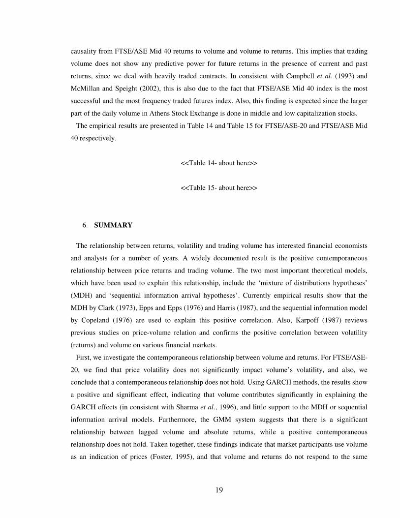
Graphical plots of return-volume coefficients are presented in Appendix 1 and Appendix 2 for

FTSE/ASE-20 and FTSE/ASE Mid 40, respectively.

5. EMPIRICAL RESULTS

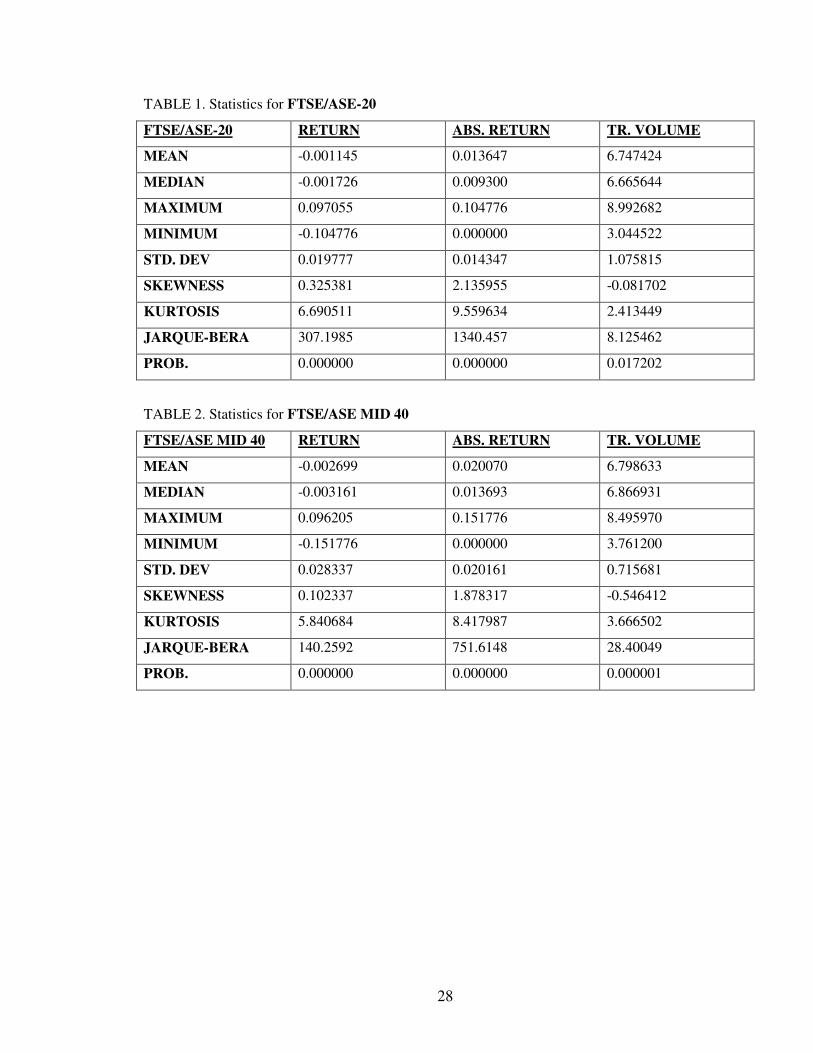
We begin the empirical analysis by first investigating the summary statistics of returns and volume

and the unit root tests. First, Table 1 provides the sample summary statistics for FTSE/ASE-20 and

Table 2 for FTSE/ASE Mid 40 stock index futures.

15

<< Table 1- about here >>


It is observed that both FTSE/ASE-20 and FTSE/ASE Mid 40 returns and absolute returns have

positive skewness, positive kurtosis and high value of J-B statistic test. This means that the

distribution is skewed to the right, and also, that the pdf is leptokurtic. Also, the J-B statistic test

suggests that the null hypothesis of normality is rejected. In addition, the results for the trading volume

indicate negative skewness, low positive kurtosis and low value of J-B statistic test. Hence, the

summary statistics for trading volumes show that the distribution is skewed to the left, and also that

the null hypothesis of normality is accepted.

• UNIT ROOT TESTS

The causality tests (and VAR models) assume that the variables (i.e. returns and trading volume) in

the system are stationary. Therefore, we test for the stationarity of returns and trading volume series.

Note that if the results indicate that the data are nonstationary then we may produce misleading results.

To test log(returns) and log(volume) for a unit root we employ the augmented Dickey-Fuller (ADF)

test. The ADF test is given by:

it

n

iitt xaxax −

=− ∆�++=∆

110 δ (15)

Table 3 shows that the null hypothesis that the futures return series and trading volume series are non-

stationary is rejected for both FTSE/ASE-20 and FTSE/ASE Mid 40 stock index futures. Hence, we

conclude that the trading volume and return series are both stationary.


I. CONTEMPORANEOUS RELATIONSHIP

• FTSE/ASE-20

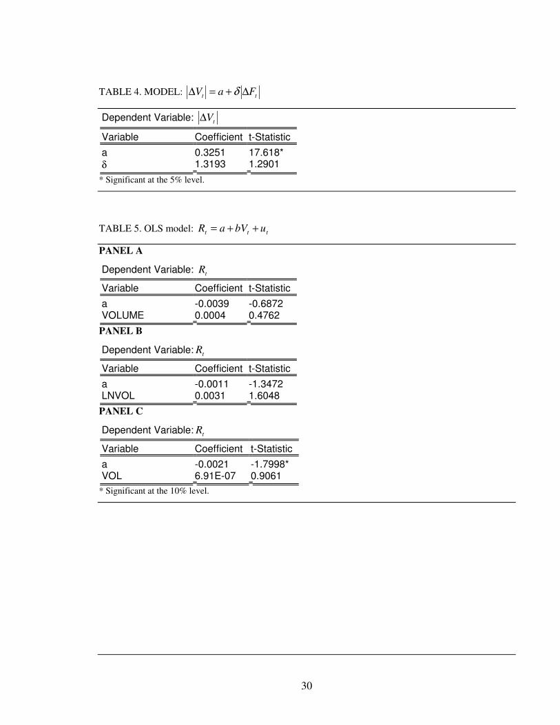
The first hypothesis investigated in this paper is that suggested in Equation 8, i.e. the volatility of

trading volume as a function of price volatility. Table 4 presents the results of this hypothesis for

16

FTSE/ASE-20 index. It shows that price volatility does not significantly impact volume’s volatility.

This finding differs with what Malliaris and Urrutia (1998) suggest for agricultural futures.


Table 5 reports the coefficients of regressing futures returns on trading volume using the simple OLS

(Equation 9). All the coefficients are positive but not significant. Therefore, we suggest that there is no

positive contemporaneous relationship between trading volume and futures returns (in all three cases).


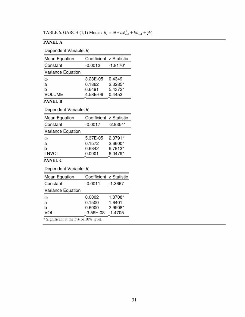
Further, to investigate whether trading volume explains the GARCH effects for futures market returns,

GARCH (1,1) model with a volume parameter in the variance equation is estimated. Table 6 reports

the results for FTSE/ASE-20 stock index futures. As can been seen, in Panels A and B the parameter

γ is positive and statistically significant (i.e. there is a positive effect), indicating also that it is

reflective of the contribution of volume in explaining the GARCH effects in futures markets returns.

In other words, the volume contributes significantly in explaining the GARCH effects (Sharma et al.,

1996).


Then, we test whether the contemporaneous relationship between trading volume and futures returns

exists using the GARCH (1,1) model with a volume parameter in the mean equation. As reported in

Table 7, the coefficients of trading volume are all positive using the GARCH (1,1) model given by

Equations (11.1) and (11.2). However, only in one case (Panel B), the coefficient is positive and

significant (i.e. there exists a positive contemporaneous relationship between trading volume and

returns).

<<Table 7- about here>>

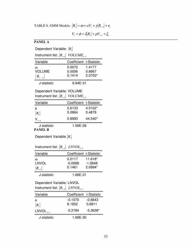
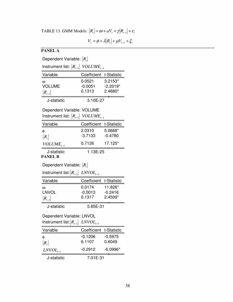
Furthermore, the results from the GMM system for FTSE/ASE-20 stock index futures are presented

in Table 8. In all cases, the coefficients a and λ are not significant, and therefore, we conclude that

there is no positive contemporaneous relationship between volatility and volume. In addition, the

results state that there is a statistically significant relationship between lagged volume and absolute

returns. The parameter µ indicates that lagged volume contains information about absolute returns.

17

Note also that, in all of the cases, the J-test is very small indicating that there exists a good fit of the

model to the data.

<< Table 8- about here>>

• FTSE/ASE MID 40

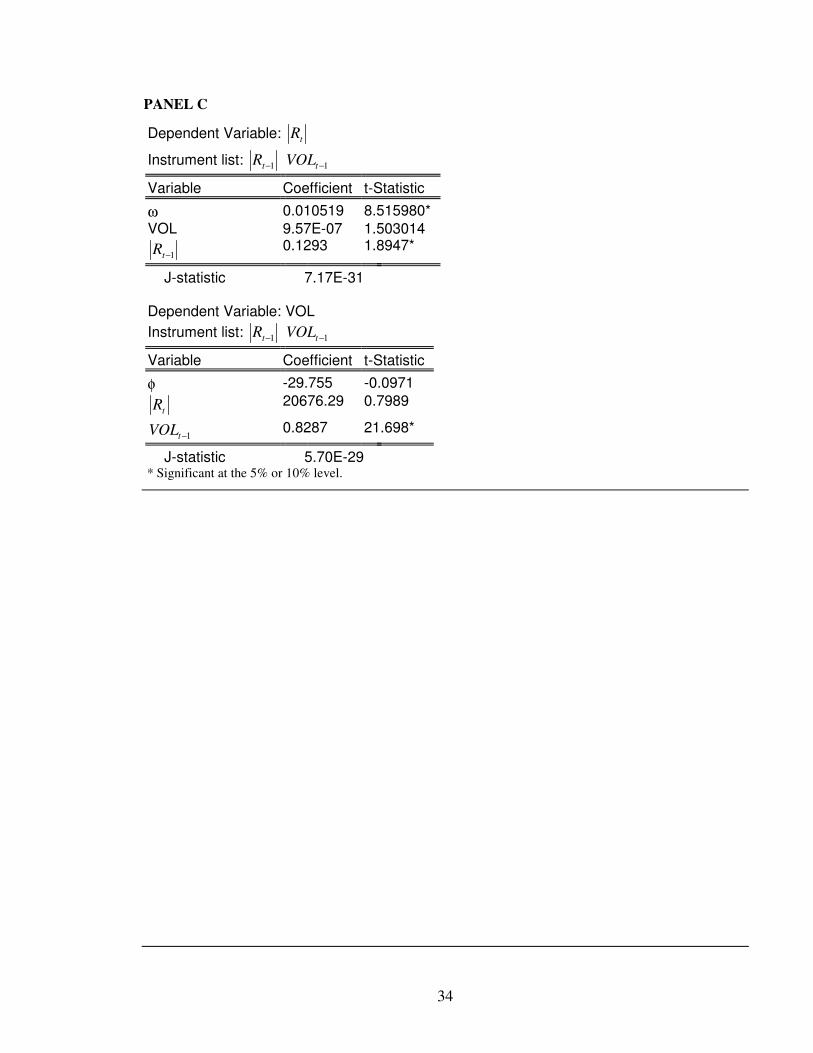
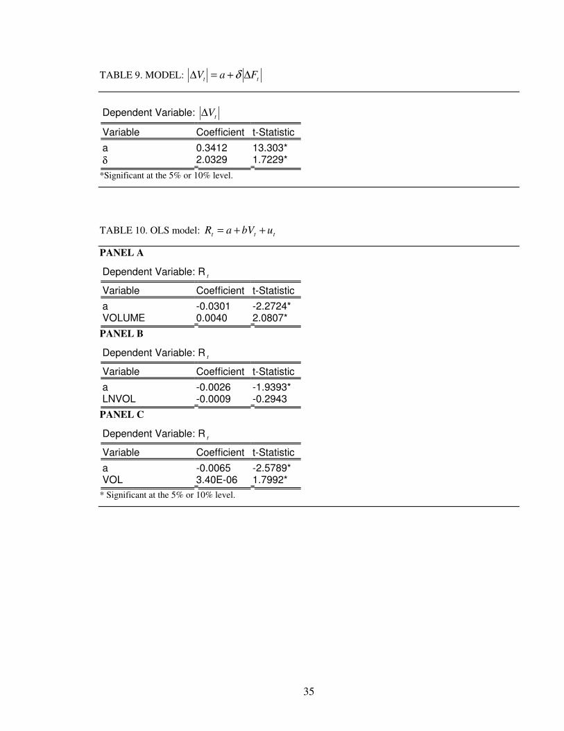
Table 9 presents the results of the first testable hypothesis suggested in Equation 8. The coefficient

of price volatility is significant, and therefore, we conclude that price volatility significantly impacts

volume’s volatility. This is consistent with the study of Malliaris and Urrutia (1998) for six

agricultural futures contracts.


Then, Table 10 shows the results obtained from the OLS model (Equation 9). As can been seen, in

Panels A and C the volume coefficient is positive and significant. So, we conclude that there exists a

positive contemporaneous relationship between trading volume and futures returns in FTSE/ASE Mid

40 stock index futures.


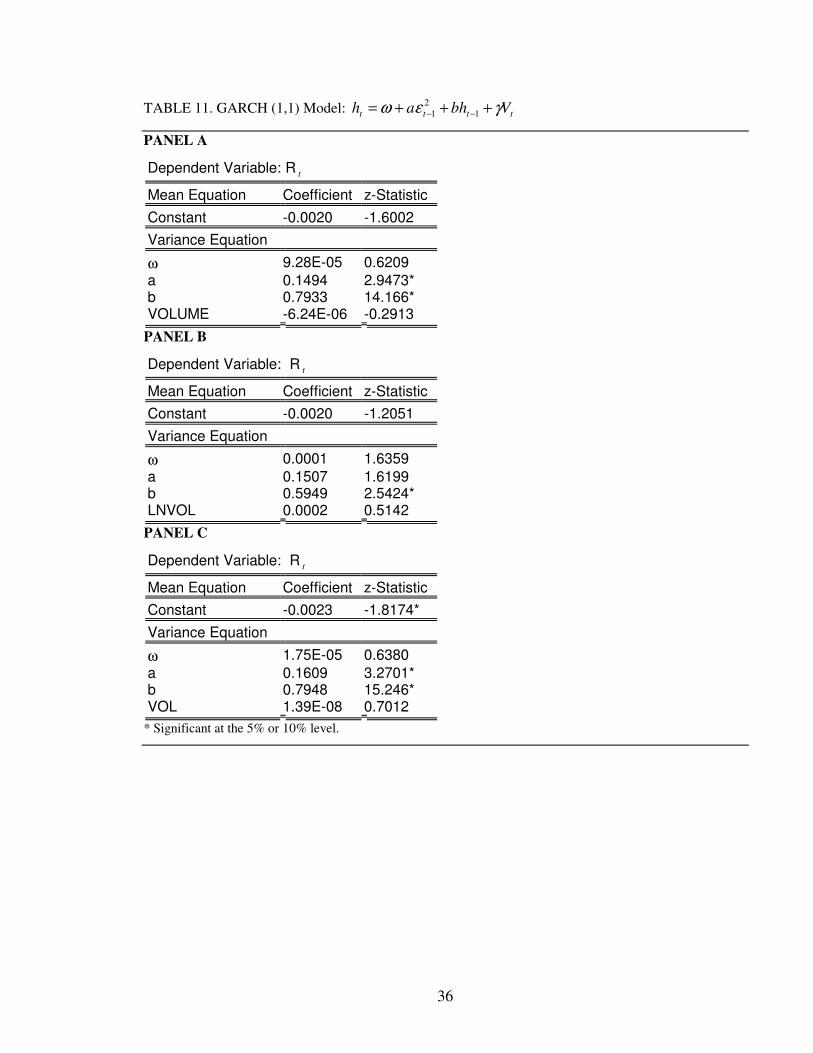
Further, Table 11 reports the results obtained from the Equation 10 following the work of Sharma et

al. (1996). It is obvious that the volume parameters are not statistically significant, and so, trading

volume does not contribute significantly in explaining the GARCH effects.


18

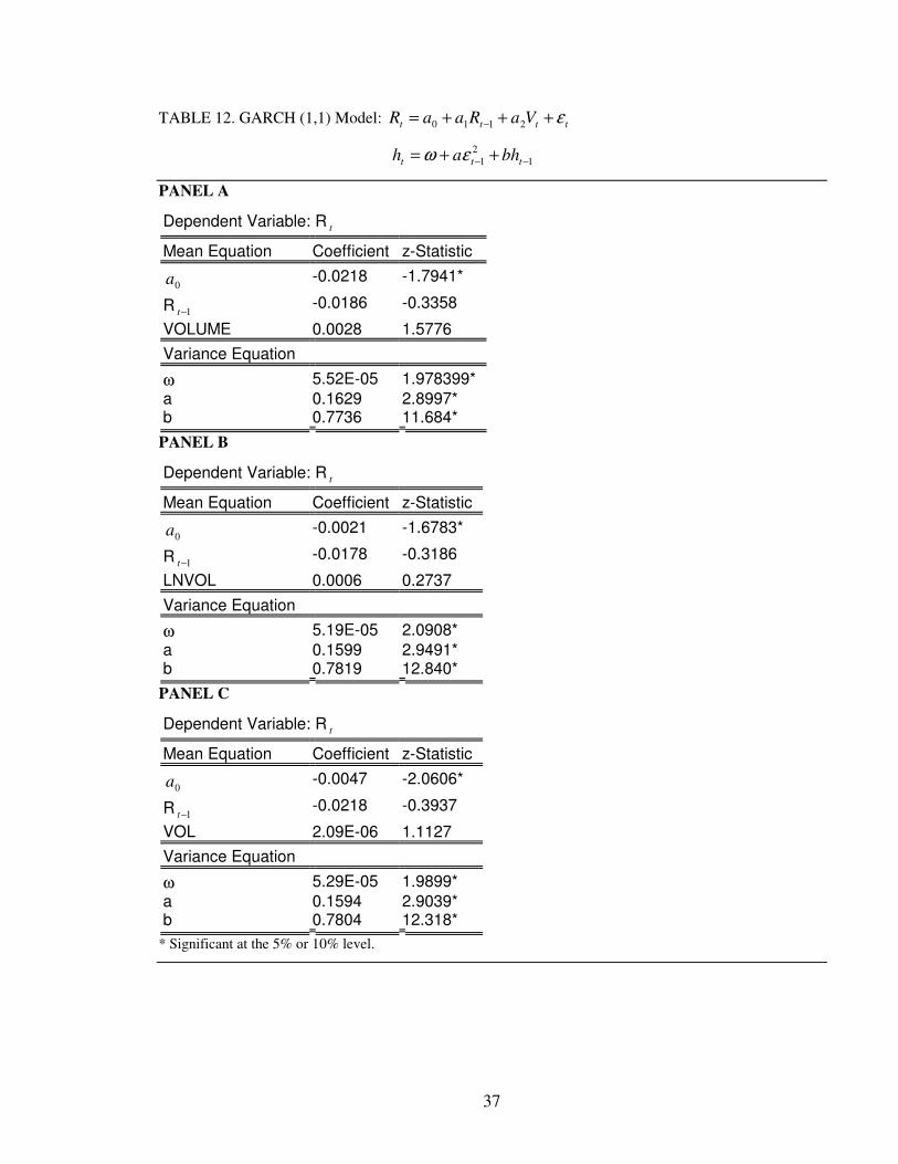
Table 12 reports the results obtained from the GARCH (1,1) model with a volume parameter in the

mean equation. The coefficients of trading volume are all positive but not significant. Hence, there is

no evidence for positive contemporaneous relationship between trading volume and futures returns in

FTSE/ASE Mid 40 index.


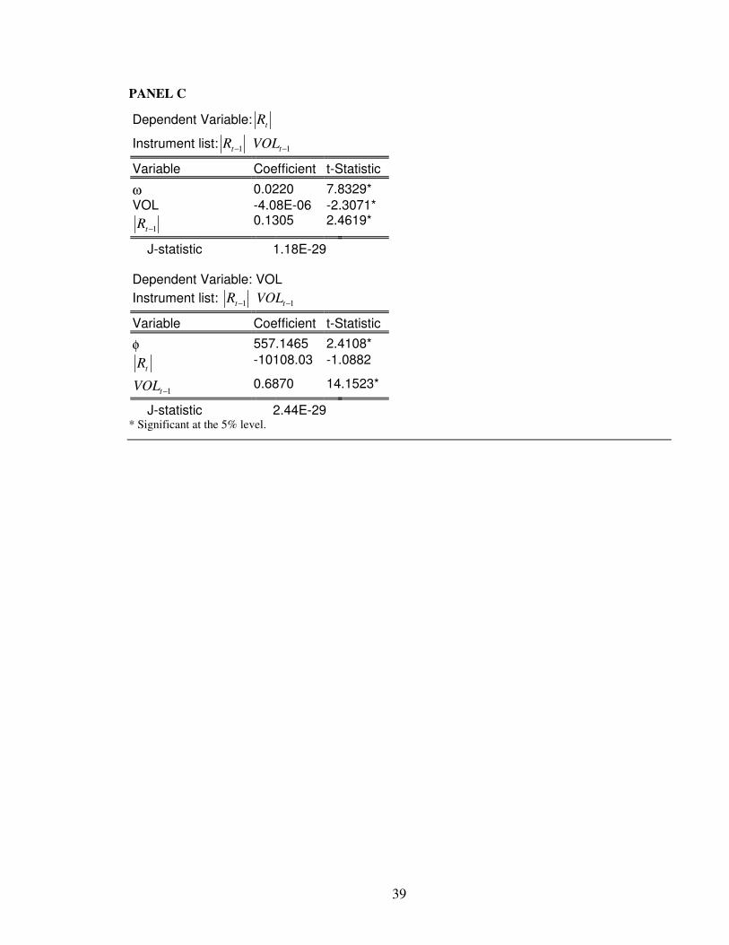
Table 13 reports the results from the GMM system. The results for the FTSE/ASE Mid 40 index

show that there is no positive and significant contemporaneous relationship between volatility and

volume. A further point of note is that the effect of lagged volume is found to be positive (Panels A

and C) in the volume equations, suggesting that the knowledge of increased current volume is a

predictor of reduced future volume. Also, the fact that the lagged return is positive in the return

equations indicates that knowledge of increased current return is a predictor of reduced future return.

In addition, the J-test statistics are very small in all of the cases, supporting a good fit to the data.


II. DYNAMIC RELATIONSHIP

As we mentioned above, in this paper we also test whether trading volume leads futures returns, or

vice versa. This is the theory behind the Granger-causality test, which is based on the fact that the

future cannot cause the present or the past.

In this study our results are mixed. For FTSE/ASE-20, there is strong evidence of bi-directional

causality (i.e. reject the null hypothesis of no Granger-causality), and therefore, there is a feedback

relation between trading volume and actual returns. Hence, we conclude that FTSE/ASE-20 index may

support the sequential arrival of information hypothesis over the MDH, and trading volume helps to

predict return and vice versa. These findings are in agreement with those of Clark (1973),

Bessembinder and Serguin (1993) and others.

However, for FTSE/ASE Mid 40, the results show evidence of accepting the null hypothesis of no

Granger-causality indicating that there is no temporal ordering in the volume-returns relationship.

Hence, FTSE/ASE Mid 40 index does not support a dynamic relationship between returns and trading

volume. Therefore, we conclude that there is no evidence of greater support to the sequential

information arrival. In other words, consistent with weak-form efficiency, we find that there is no

19

causality from FTSE/ASE Mid 40 returns to volume and volume to returns. This implies that trading

volume does not show any predictive power for future returns in the presence of current and past

returns, since we deal with heavily traded contracts. In consistent with Campbell et al. (1993) and

McMillan and Speight (2002), this is also due to the fact that FTSE/ASE Mid 40 index is the most

successful and the most frequency traded futures index. Also, this finding is expected since the larger

part of the daily volume in Athens Stock Exchange is done in middle and low capitalization stocks.

The empirical results are presented in Table 14 and Table 15 for FTSE/ASE-20 and FTSE/ASE Mid

40 respectively.



6. SUMMARY

The relationship between returns, volatility and trading volume has interested financial economists

and analysts for a number of years. A widely documented result is the positive contemporaneous

relationship between price returns and trading volume. The two most important theoretical models,

which have been used to explain this relationship, include the ‘mixture of distributions hypotheses’

(MDH) and ‘sequential information arrival hypotheses’. Currently empirical results show that the

MDH by Clark (1973), Epps and Epps (1976) and Harris (1987), and the sequential information model

by Copeland (1976) are used to explain this positive correlation. Also, Karpoff (1987) reviews

previous studies on price-volume relation and confirms the positive correlation between volatility

(returns) and volume on various financial markets.

First, we investigate the contemporaneous relationship between volume and returns. For FTSE/ASE-

20, we find that price volatility does not significantly impact volume’s volatility, and also, we

conclude that a contemporaneous relationship does not hold. Using GARCH methods, the results show

a positive and significant effect, indicating that volume contributes significantly in explaining the

GARCH effects (in consistent with Sharma et al., 1996), and little support to the MDH or sequential

information arrival models. Furthermore, the GMM system suggests that there is a significant

relationship between lagged volume and absolute returns, while a positive contemporaneous

relationship does not hold. Taken together, these findings indicate that market participants use volume

as an indication of prices (Foster, 1995), and that volume and returns do not respond to the same

20

exogenous variable in the GMM system, the daily flow of information to the market. The latter is in

contrast with Ciner (2001).

For FTSE/ASE Mid 40, the results are mixed. The price volatility significantly impacts volume’s

volatility, and also, a positive contemporaneous relationship holds. These results are in contrast with

previous results for FTSE/ASE-20. However, both GARCH and GMM methods confirm that there is

no evidence for positive relationship between trading volume and returns.

This study also investigates the dynamic relationship between trading volume and actual returns for

Greek index futures. For FTSE/ASE-20, using linear Granger causality tests, we conclude that past

volume provides information on current returns, and past returns contains information on current

volume. Therefore, the bi-directional causality suggests that speculators pay attention to price changes

and changes in trading volume. In other words, the finding of strong bi-directional futures returns-

volume causal relationships implies that knowledge of current trading volume improves the ability to

forecast futures returns. These results are in line with those of Grammatikos and Saunders (1986),

Bessembinder and Seguin (1993), Malliaris and Urrutia (1998), Gwilym et al. (1999) and McMillan

and Speight (2002), who report a bi-directional relationship between volume and price variability.

Furthermore, the fact that there is causality from volume to returns indicates that a financial trader

“takes volume to make prices move” (Ciner; 2001, p. 3). Hence, for the FTSE/ASE-20 index futures

market we show evidence for the sequential arrival of information hypothesis.

However, for FTSE/ASE Mid 40, we find that there is no causality from volume to returns and

returns to volume, consistent with weak-form efficiency. This finding is consistent with McCarthy and

Najand (1993), Kocagil and Shachmurove (1998), Bhar and Malliaris (1998), Walls (1999) and

Gwilym et al. (1999) for daily futures data. They suggest that major US and UK (LIFFE) futures

markets are weak-form efficient. The lack of causality (and efficiency) between returns and volume is

possibly explained by the fact that the FTSE/ASE Mid 40 index is the most frequency traded stock

index in Athens Stock Exchange.

Overall, statistical analysis shows that trading volume and returns do not clear support a positive

contemporaneous relationship on Greek futures market. On the other hand, for FTSE/ASE-20, the

dynamic models show a bi-directional Granger causality (feedback) between volume and actual

returns. However, for FTSE/ASE Mid 40, the results indicate that returns do not Granger cause

volume and vice versa.

The results of this study should be useful to financial researchers-analysts, practitioners and

derivative (futures) market participants whose success depends on the ability to forecast price

movements in the ASE and ADEX.

21

APPENDIX 1

FTSE/ASE-20

Fig. 1

0.00

0.02

0.04

0.06

0.08

0.10

0.12

100 200 300 400 500

ABS. RETURNFig. 2

-0.15

-0.10

-0.05

0.00

0.05

0.10

100 200 300 400 500

RETURN

Fig. 3

-2

-1

0

1

2

3

50 100 150 200 250 300 350 400 450 500

LNVOLFig. 4

0

2000

4000

6000

8000

10000

100 200 300 400 500

VOL

Fig. 5

2

4

6

8

10

50 100 150 200 250 300 350 400 450 500

VOLUME

* Graphical plots of abs. return, return, lnvol, vol and volume for FTSE/ASE-20.

22

APPENDIX 2

FTSE/ASE MID 40

Fig. 1

0.00

0.04

0.08

0.12

0.16

50 100 150 200 250 300 350 400

ABS. RETURNFig. 2

-0.20

-0.15

-0.10

-0.05

0.00

0.05

0.10

50 100 150 200 250 300 350 400

RETURN

Fig. 3

-3

-2

-1

0

1

2

3

50 100 150 200 250 300 350 400

LNVOLFig. 4

0

1000

2000

3000

4000

5000

50 100 150 200 250 300 350 400

VOL

Fig. 5

3

4

5

6

7

8

9

50 100 150 200 250 300 350 400

VOLUME

* Graphical plots of abs. return, return, lnvol, vol and volume for FTSE/ASE Mid 40.

23

REFERENCES

Anderson, R. W. (1985), ‘Some Determinants of the Volatility of Futures Prices’, Journal of Futures

Markets, 5, 331-348.

Antoniou, A., Ergul, N., Holmes, P. and Priestley, R. (1997), ‘Technical analysis, trading volume and

market efficiency: evidence from an emerging market’, Applied Financial Economics, 7, 361-365.

Bessembinder, H. and Seguin, P. J. (1992), ‘Futures trading activity and stock price volatility’,

Journal of Finance, 47, 2015-2034.

Bessembinder, H. and Seguin, P. J. (1993), ‘Price Volatility, Trading Volume, and Market Depth:

Evidence from Futures Markets’, Journal of Financial and Quantitative Analysis, 28, 21-39.

Bhar, R. and Malliaris, A. G. (1998), ‘Volume and volatility in foreign currency futures markets’,

Review of Quantitative Finance and Accounting, 10, 285-302.

Board, J. L. G. and Sutcliffe, C. M. S. (1990), ‘Information, volatility, volume and maturity: an

investigation of stock index futures’, Review of Futures Markets, 9.

Bollerslev, T. (1986), ‘Generalised Autoregressive Conditional Heteroskedasticity’, Journal of

Econometrics, 30, 307-328.

Brailsford, T. J. (1994), ‘The Empirical Relationship Between Trading Volume, Returns and

Volatility’, Research Paper 94-01, Department of Accounting and Finance, University of

Melbourne.

Brailsford, T. J. (1996), ‘The Empirical Relationship Between Trading Volume, Returns and

Volatility’, Accounting and Finance, 36, 89-111.

Campbell, J., Grossman, S. and Wang, J. (1993), ‘Trading volume and serial correlation in stock

returns’, Quarterly Journal of Economics, 108, 905-939.

Chen, Y-J, Duan, J-C, and Hung, M-W (1999), ‘Volatility and Maturity Effects in the Nikkei Index

Futures’, Journal of Futures Markets, 19, 895-909.

Ciner, C. (2001), ‘Information content of volume: an investigation of Tokyo commodity futures

markets’, Pacific-Basin Finance Journal, Article in press.

Clark, P. (1973), ‘A subordinated stochastic process model with finite variance for speculative prices’,

Econometrica, 41, 135-155.

Copeland, T. (1976), ‘A model of asset trading under the assumption of sequential information

arrival’, Journal of Finance, 31, 1149-1168.

Cornell, B. (1981), ‘The Relationship between Volume and Price Variability in Futures Markets’,

Journal of Futures Markets, 1, 303-316.

24

Daigler, R. T. and Wiley, M. K. (1999), ‘The Impact of Trader Type on the Futures Volatility-Volume

Relation’, Journal of Finance, 6, 2297-2316.

Enders, W. (1995), ‘Applied Econometric Time Series’, John Wiley & Sons, New York.

Epps, T. and Epps, M. (1976), The stochastic dependence of security price changes and transaction

volumes: implications for the Mixture-of-Distributions hypothesis’, Econometrica, 44, 305-321.

Faff, R. W. and McKenzie, M. D. (2002), ‘The Impact of Stock Index Futures Trading on Daily

Returns Seasonality: A Multicountry Study’, Journal of Business, 75, 95-125.

Foster, A. J. (1995), ‘Volume-volatility relationships for crude oil futures markets’, Journal of Futures

Markets, 15, 929-951.

Gallant, A. R., Rossi, P. E. and Tauchen, G. (1992), ‘Stock prices and volume’, Review of Financial

Studies, 5, 199-242.

Gallant, A. R., Rossi, P. E. and Tauchen, G. (1993), ‘Nonlinear dynamic structures’, Econometrica,

61, 871-907.

Galloway, T. and Kolb, R. W. (1996), ‘Futures prices and the maturity effect’, Journal of Futures

Markets, 16, 809-828.

Grammatikos, T. and Saunders, A. (1986), ‘Futures Price Variability: A Test of Maturity and Volume

Effects’, Journal of Business, 59, 319-330.

Gwilym, O., McMillan, D. and Speight, A. (1999), ‘The intraday relationship between volume and

volatility in LIFFE futures markets’, Applied Financial Economics, 9, 593-604.

Han, L. M., Kling, J. L. and Sell, C. W. (1999), ‘Foreign Exchange Futures Volatility: Day-of-the-

Week, Intraday and Maturity Patterns in the Presence of Macroeconomic Announcements’, Journal

of Futures Markets, 19, 665-693.

Hansen, L. P. (1982), ‘Large sample properties of generalized method of moments estimators’,

Econometrica, 50, 1029-1054.

Harris, L. (1983/1984), ‘The joint distribution of speculative prices and of daily trading volume’,

Working paper no. 34-84, Los Angeles: University of Southern California, Department of Finance

and Business Economics.

Harris, L. (1984), ‘Transactions data tests of the mixture of distributions hypothesis’, Working paper

no. 31-84, Los Angeles: University of Southern California, Department of Finance and Business

Economics.

Harris, L. (1986), ‘Cross-security tests of the Mixture of Distributions hypothesis’, Journal of

financial and Quantitative Analysis, 21, 39-46.

Harris, L. (1987), ‘Transaction data tests of the Mixture of Distributions Hypothesis’, Journal of

Financial and Quantitative Analysis, 22, 127-141.

25

Harris, M. and Raviv, A. (1993), ‘Differences of opinion make a horse race’, Review of Financial

Studies, 6, 473-506.

Herbert, J. H. (1995), ‘Trading Volume, Maturity and Natural Gas Futures Price Volatility’, Energy

Economics, 17, 293-299.

Hiemstra, C. and Jones, J. D. (1994), ‘Testing for linear and non-linear Granger causality in the stock

price-volume relationship’, Journal of Finance, 49, 1639-64.

Hogan, K. C. JR., Kronner, K. F. and Sultan, J. (1997), ‘Program Trading, Nonprogram Trading, and

Market Volatility’, Journal of Futures Markets, 17, 733-756.

Jacobs, M. JR. and Onochie, J. (1998), ‘A Bivariate Generalized Autoregressive Conditional

Heteroscedasticity-in-Mean Study of the Relationship between Return Variability and Trading

Volume in International Futures Markets’, Journal of Futures Markets, 18, 379-397.

Johnson, J. (1998), ‘Does the Samuelson Effect Hold for SPI Futures?’, Department of Accounting

and Finance, University of Western Australia, Working Paper.

Karpoff, J. M. (1986), ‘A theory of trading volume’, Journal of Finance, 41, 1069-1082.

Karpoff, J. M. (1987), ‘The Relation Between Price Changes and Trading Volume: A Survey’,

Journal of Financial and Quantitative Analysis, 22, 109-126.

Kawaller, I. G., Koch, P. D. and Koch, T. W. (1990), ‘Intraday relationships between volatility in

S&P500 futures prices and volatility in the S&P index’, Journal of Banking and Finance, 14, 373-

397.

Kocagil, A. E. and Shachmurove, Y. (1998), ‘Return-Volume Dynamics in Futures Markets’, Journal

of Futures Markets, 18, 399-426.

Lamoureux, C. G. and Lastrapes, W. D. (1990), ‘Heteroskedasticity in stock returns data: volume

versus GARCH effects’, Journal of Finance, 45, 221-29.

Malliaris, A. G. and Urrutia, J. L. (1998), ‘Volume and Price Relationships: Hypotheses and Testing

for Agricultural Futures’, Journal of Futures Markets, 18, 53-72.

McCarthy, J. and Najand, M. (1993), ‘State space modelling of price and volume dependence:

evidence from currency futures’, Journal of Futures Markets, 13, 335-44.

McMillan, D. and Speight, A. (2002), ‘Return-volume dynamics in UK futures’, Applied Financial

Economics, preview article, 1-7.

Merrick, J. J. (1987), ‘Volume determination in stock and stock index futures markets: an analysis of

arbitrage and volatility effects’, Journal of Futures Markets, 7, 483-496.

Milonas, N. T. (1986), ‘Price Variability and the Maturity Effect in Futures Markets’, Journal of

Futures Markets, 6, 443-460.

26

Montalvo, J. G. (1999), ‘Volume versus GARCH effects reconsidered: an application to the Spanish

Government Bond Futures Market’, Applied Financial Economics, 9, 469-475.

Moosa, I. A. and Bollen, B. (2001), ‘Is there a maturity effect in the price of the S&P 500 futures

contract?’, Applied Economics Letters, 8, 693-695.

Najand, M. and Yung, K. (1991), ‘A GARCH examination of the relationship between volume and

price variability in futures markets’, Journal of Futures Markets, 11, 613-621.

Najand, M. and Yung, K. (1994), ‘Conditional Heteroskedasticity and the Weekend Effect in S&P 500

Index Futures’, Journal of Business Finance & Accounting, 21, 603-612.

Pilar, C., and Rafael, S. (2002), ‘Does derivatives trading destabilize the underlying assets? Evidence

from the Spanish stock market’, Applied Economics Letters, Vol 9, No 2, 107-110.

Pindyck, R.S. and Rubinfeld, D.L. (1998), ‘Econometric models and economic forecasts’, 4th Ed.,

Irwin McGraw-Hill.

Ragunathan, V. and Peker, A. (1997), ‘Price variability, trading volume and market depth: evidence

from the Australian futures market’, Applied Financial Economics, 7, 447-454.

Richardson, M. and Smith, T. (1994), ‘A direct test of the mixture distributions hypothesis: measuring

the daily flow of information’, Journal of Financial and Quantitative Analysis, 29, 101-116.

Rutledge, D. J. S. (1977/78), ‘Trading volume and price variability: new evidence on the price effects

of speculation’, in Futures Markets: Their Establishment and Performance (ed. B. A. Goss),

Croom Helm, London, 1986, 137-156.

Schwert, G. W. (1990), ‘Stock volatility and the crash of ‘87’, Review of Financial Studies, 3, 77-102.

Serletis, A. (1992), ‘Maturity effects in energy futures’, Energy Economics, 14, 150-157.

Sharma, J. L., Mougoue, M. and Kamath, R. (1996), ‘Heteroscedasticity in stock market indicator

return data: volume versus GARCH effects’, Applied Financial Economics, 6, 337-342.

Sutcliffe, C. M. S. (1993), ‘Stock Index Futures: Theories and International Evidence’, Chapman &

Hall.

Tauchen, G. E. and Pitts, M. (1983), ‘The price variability volume relationship on speculative

markets’, Econometrica, 51, 485-505.

Tauchen, G. E., Zhang, H. and Liu, M. (1996), ‘Volume volatility and leverage: a dynamic

relationship’, Journal of Econometrics, 74, 177-208.

Walls, W. D. (1999), ‘Volatility, volume and maturity in electricity futures’, Applied Financial

Economics, 9, 283-287.

Wang, G. H. K. and Yau, J. (2000), ‘Trading Volume, Bid-Ask Spread, and Price Volatility in Futures

Markets’, Journal of Futures Markets, 20, 943-970.

27

Watanabe, T. (2001), ‘Price volatility, trading volume, and market depth: evidence from the Japanese

stock index futures market’, Applied Financial Economics, 11, 651-658.

Wiley, M. K. and Daigler, R. T. (1998), ‘Volume Relationships among Types of Traders in the

Financial Futures Markets’, Journal of Futures Markets, 18, 91-113.

Wiley, M. K. and Daigler, R. T. (1999), ‘A Bivariate GARCH Approach to the Futures Volume-

Volatility Issue’, Article Presented at the Eastern Finance Association Meetings, Florida.

Yang, S. R. and Brorsen, B. W. (1993), ‘Nonlinear Dynamics of Daily Futures Prices: Conditional

Heteroskedasticity or Chaos?’, Journal of Futures Markets, 13, 175-191.

Ying, C. C. (1966), ‘Stock Market Prices and Volumes of Sales’, Econometrica, 34, 676-686.

28

TABLE 1. Statistics for FTSE/ASE-20

FTSE/ASE-20 RETURN ABS. RETURN TR. VOLUME

MEAN -0.001145 0.013647 6.747424

MEDIAN -0.001726 0.009300 6.665644

MAXIMUM 0.097055 0.104776 8.992682

MINIMUM -0.104776 0.000000 3.044522

STD. DEV 0.019777 0.014347 1.075815

SKEWNESS 0.325381 2.135955 -0.081702

KURTOSIS 6.690511 9.559634 2.413449

JARQUE-BERA 307.1985 1340.457 8.125462

PROB. 0.000000 0.000000 0.017202

TABLE 2. Statistics for FTSE/ASE MID 40

FTSE/ASE MID 40 RETURN ABS. RETURN TR. VOLUME

MEAN -0.002699 0.020070 6.798633

MEDIAN -0.003161 0.013693 6.866931

MAXIMUM 0.096205 0.151776 8.495970

MINIMUM -0.151776 0.000000 3.761200

STD. DEV 0.028337 0.020161 0.715681

SKEWNESS 0.102337 1.878317 -0.546412

KURTOSIS 5.840684 8.417987 3.666502

JARQUE-BERA 140.2592 751.6148 28.40049

PROB. 0.000000 0.000000 0.000001

29

TABLE 3. Unit Root Tests FTSE/ASE-20

INDEX

ADF (RETURN)

Critical Values:

1%: -3.4452

5%: 2.8674

10%: 2.5699

ADF (VOLUME)

Critical Values:

1%: -3.4452

5%: -2.8674

10%: -2.5699

LAGS 3 3

ADF -0.777813 -2.737684

1ST DIFF. ADF -11.55063 -15.37652

FTSE/ASE MID 40

INDEX

ADF (RETURN)

Critical Values:

1%: -3.4483

5%: 2.8688

10%: 2.5706

ADF (VOLUME)

Critical Values:

1%: -3.4484

5%: -2.8688

10%: -2.5706

LAGS 2 6

ADF -1.954468 -3.535182

1ST DIFF. ADF -12.81365 -

30

TABLE 4. MODEL: tt FaV ∆+=∆ δ

Dependent Variable: tV∆

Variable Coefficient t-Statistic a 0.3251 17.618* δ 1.3193 1.2901

* Significant at the 5% level.

TABLE 5. OLS model: ttt ubVaR ++=

PANEL A

Dependent Variable: tR

Variable Coefficient t-Statistic a -0.0039 -0.6872 VOLUME 0.0004 0.4762

PANEL B


Variable Coefficient t-Statistic a -0.0011 -1.3472 LNVOL 0.0031 1.6048

PANEL C


Variable Coefficient t-Statistic a -0.0021 -1.7998* VOL 6.91E-07 0.9061

* Significant at the 10% level.

31

TABLE 6. GARCH (1,1) Model: tttt Vbhah γεω +++= −− 12

1

PANEL A


Mean Equation Coefficient z-Statistic Constant -0.0012 -1.8170* Variance Equation

ω 3.23E-05 0.4349 a 0.1862 2.3285* b 0.6491 5.4372* VOLUME 4.58E-06 0.4453

PANEL B



ω 5.37E-05 2.3791* a 0.1572 2.6600* b 0.6842 6.7913* LNVOL 0.0001 6.0479*

PANEL C


Mean Equation Coefficient z-Statistic Constant -0.0011 -1.3667 Variance Equation

ω 0.0002 1.8708* a 0.1500 1.6401 b 0.6000 2.9508* VOL -3.56E-08 -1.4705

* Significant at the 5% or 10% level.

32

TABLE 7. GARCH (1,1) Model: tttt VaRaaR ε+++= − 2110

12

1 −− ++= ttt bhah εω

PANEL A


Mean Equation Coefficient z-Statistic

0a -0.0015 -0.3164

1−tR 0.1110 2.4283*

VOLUME 6.33E-05 0.0845 Variance Equation

ω 5.54E-05 2.1993* a 0.1702 2.3521* b 0.6833 6.3203*

PANEL B



0a -0.0012 -1.6922*

1−tR 0.1124 2.4457*

LNVOL 0.0038 2.0897* Variance Equation

ω 5.14E-05 2.1855* a 0.1668 2.3788* b 0.6953 6.6864*

PANEL C



0a -0.0014 -1.4298

1−tR 0.1113 2.4407*

VOL 2.08E-07 0.3222 Variance Equation

ω 5.49E-05 2.1872* a 0.1689 2.3384* b 0.6857 6.3398*


33

TABLE 8. GMM Models: tttt RaVR εγω +++= −1

tttt VRV ξµλφ +++= −1

PANEL A


Instrument list: 1−tR 1−tVOLUME

Variable Coefficient t-Statistic

ω 0.0072 1.4177 VOLUME 0.0006 0.8867

1−tR 0.1414 2.0703*

J-statistic 9.94E-31 Dependent Variable: VOLUME Instrument list: 1−tR 1−tVOLUME


φ 0.6133 4.5102*

tR 5.0864 0.4878

V 1−t 0.8993 44.540*

J-statistic 1.56E-26 PANEL B

Dependent Variable: tR Instrument list: 1−tR 1−tLNVOL


ω 0.0117 11.618* LNVOL -0.0068 -1.0848

1−tR 0.1461 2.0994*

J-statistic 1.68E-31 Dependent Variable: LNVOL Instrument list: 1−tR 1−tLNVOL


φ -0.1070 -0.6643

tR 8.1852 0.6811

LNVOL 1−t -0.2784 -5.3638*

J-statistic 1.68E-30

34

PANEL C


Instrument list: 1−tR 1−tVOL


ω 0.010519 8.515980* VOL 9.57E-07 1.503014

1−tR 0.1293 1.8947*

J-statistic 7.17E-31 Dependent Variable: VOL Instrument list: 1−tR 1−tVOL


φ -29.755 -0.0971

tR 20676.29 0.7989

1−tVOL 0.8287 21.698*

J-statistic 5.70E-29 * Significant at the 5% or 10% level.

35

TABLE 9. MODEL: tt FaV ∆+=∆ δ

Dependent Variable: tV∆

Variable Coefficient t-Statistic a 0.3412 13.303* δ 2.0329 1.7229*

*Significant at the 5% or 10% level.

TABLE 10. OLS model: ttt ubVaR ++=

PANEL A

Dependent Variable: R t

Variable Coefficient t-Statistic a -0.0301 -2.2724* VOLUME 0.0040 2.0807*

PANEL B


Variable Coefficient t-Statistic a -0.0026 -1.9393* LNVOL -0.0009 -0.2943

PANEL C


Variable Coefficient t-Statistic a -0.0065 -2.5789* VOL 3.40E-06 1.7992*


36

TABLE 11. GARCH (1,1) Model: tttt Vbhah γεω +++= −− 12

1

PANEL A



ω 9.28E-05 0.6209 a 0.1494 2.9473* b 0.7933 14.166* VOLUME -6.24E-06 -0.2913

PANEL B



ω 0.0001 1.6359 a 0.1507 1.6199 b 0.5949 2.5424* LNVOL 0.0002 0.5142

PANEL C



ω 1.75E-05 0.6380 a 0.1609 3.2701* b 0.7948 15.246* VOL 1.39E-08 0.7012


37

TABLE 12. GARCH (1,1) Model: tttt VaRaaR ε+++= − 2110

12

1 −− ++= ttt bhah εω

PANEL A



0a -0.0218 -1.7941*

R 1−t -0.0186 -0.3358

VOLUME 0.0028 1.5776 Variance Equation

ω 5.52E-05 1.978399* a 0.1629 2.8997* b 0.7736 11.684*

PANEL B



0a -0.0021 -1.6783*

R 1−t -0.0178 -0.3186

LNVOL 0.0006 0.2737 Variance Equation

ω 5.19E-05 2.0908* a 0.1599 2.9491* b 0.7819 12.840*

PANEL C



0a -0.0047 -2.0606*

R 1−t -0.0218 -0.3937

VOL 2.09E-06 1.1127 Variance Equation

ω 5.29E-05 1.9899* a 0.1594 2.9039* b 0.7804 12.318*


38

TABLE 13. GMM Models: tttt RaVR εγω +++= −1

tttt VRV ξµλφ +++= −1

PANEL A


Instrument list: 1−tR 1−tVOLUME


ω 0.0521 3.2153* VOLUME -0.0051 -2.2019*

1−tR 0.1313 2.4680*

J-statistic 3.10E-27 Dependent Variable: VOLUME Instrument list: 1−tR 1−tVOLUME


φ 2.0310 5.0668*

tR -3.7133 -0.4780

1−tVOLUME 0.7126 17.125*

J-statistic 1.13E-25 PANEL B


Instrument list: 1−tR 1−tLNVOL


ω 0.0174 11.826* LNVOL -0.0013 -0.2416

1−tR 0.1317 2.4509*

J-statistic 5.85E-31 Dependent Variable: LNVOL Instrument list: 1−tR 1−tLNVOL


φ -0.1206 -0.5975

tR 6.1107 0.6049

1−tLNVOL -0.2912 -6.0996*

J-statistic 7.01E-31

39

PANEL C


Instrument list: 1−tR 1−tVOL


ω 0.0220 7.8329* VOL -4.08E-06 -2.3071*

1−tR 0.1305 2.4619*

J-statistic 1.18E-29 Dependent Variable: VOL Instrument list: 1−tR 1−tVOL


φ 557.1465 2.4108*

tR -10108.03 -1.0882

1−tVOL 0.6870 14.1523*

J-statistic 2.44E-29 * Significant at the 5% level.

40

TABLE 14. Pairwise Granger Causality Tests (FTSE/ASE-20)

PANEL A

Null Hypothesis: Obs F-Statistic Probability RETURN does not Granger Cause VOLUME 521 2.68663 0.0307* VOLUME does not Granger Cause RETURN 3.16840 0.0137*

PANEL B

Null Hypothesis: Obs F-Statistic Probability RETURN does not Granger Cause LNVOL 521 2.78645 0.0260* LNVOL does not Granger Cause RETURN 3.33706 0.0103*

PANEL C

Null Hypothesis: Obs F-Statistic Probability RETURN does not Granger Cause VOL 521 2.00533 0.0925 VOL does not Granger Cause RETURN 2.89476 0.0217*

*Reject the Ho.

TABLE 15. Pairwise Granger Causality Tests (FTSE/ASE MID 40)

PANEL A

Null Hypothesis: Obs F-Statistic Probability VOLUME does not Granger Cause RETURN 411 2.00146 0.0935 RETURN does not Granger Cause VOLUME 0.81611 0.5154

PANEL B

Null Hypothesis: Obs F-Statistic Probability LNVOL does not Granger Cause RETURN 411 0.50039 0.7354 RETURN does not Granger Cause LNVOL 0.76051 0.5514

PANEL C

Null Hypothesis: Obs F-Statistic Probability VOL does not Granger Cause RETURN 411 1.19304 0.3132 RETURN does not Granger Cause VOL 0.27042 0.8969

the relationship between trading volume, returns and ... · pdf file1 the relationship between...

Documents