analysis of the audit framework focusing on inherent risk

University of Mississippi University of Mississippi

eGrove eGrove

Proceedings of the University of Kansas Symposium on Auditing Problems Deloitte Collection

1-1-1984

Analysis of the audit framework focusing on inherent risk and the Analysis of the audit framework focusing on inherent risk and the

role of statistical sampling in compliance testing role of statistical sampling in compliance testing

Donald A. Leslie

Follow this and additional works at: https://egrove.olemiss.edu/dl_proceedings

Part of the Accounting Commons, and the Taxation Commons

Recommended Citation Recommended Citation Auditing Symposium VII: Proceedings of the 1984 Touche Ross/University of Kansas Symposium on Auditing Problems, pp. 089-125;

This Article is brought to you for free and open access by the Deloitte Collection at eGrove. It has been accepted for inclusion in Proceedings of the University of Kansas Symposium on Auditing Problems by an authorized administrator of eGrove. For more information, please contact [email protected].

https://egrove.olemiss.edu/

https://egrove.olemiss.edu/dl_proceedings

https://egrove.olemiss.edu/dl_proceedings

https://egrove.olemiss.edu/deloitte

https://egrove.olemiss.edu/dl_proceedings?utm_source=egrove.olemiss.edu%2Fdl_proceedings%2F162&utm_medium=PDF&utm_campaign=PDFCoverPages

http://network.bepress.com/hgg/discipline/625?utm_source=egrove.olemiss.edu%2Fdl_proceedings%2F162&utm_medium=PDF&utm_campaign=PDFCoverPages

http://network.bepress.com/hgg/discipline/643?utm_source=egrove.olemiss.edu%2Fdl_proceedings%2F162&utm_medium=PDF&utm_campaign=PDFCoverPages

mailto:[email protected]

5 An Analysis of the Audit Framework Focusing on Inherent Risk and the Role of Statistical Sampling in Compliance Testing

Donald A. Leslie Clarkson Gordon

Auditors are a loyal brotherhood of arithmetic wizards who when their profession starts to go down the pipe . . . band together and disagree with one another.

with apologies to J. Hart

The highly competitive professional environment that has developed in the U.S. over the past 10 years has spread like a cancer throughout most of the world. As a result, meaningful professional standards are currently more important to the profession's survival than at any time in its relatively short existence. Competition can and should be healthy for a profession, ensuring that users of the professional services receive "value for their money" and that the profession keeps "abreast of modern technology." Unfortunately, far too many users of accounting services are tending to treat them as simple commodities that can be purchased like "groceries on a shelf." Some observers are of the opinion that "the standard audit is increasingly viewed as a simple commodity item" and that "a lot of companies are starting to treat their accountants the way they treat their janitorial service."1 Extracts from a recent interview with Ralph Walters on the subject of accounting regulation and competition in the profession in the U.S. are set out in the Appendix.

The purpose of this paper is to assist the profession in establishing a common audit objective.* In order to ensure that readers do not misinterpret my intent, I should make it clear at the outset that I do not believe that it is necessary for all auditors to carry out their audits in exactly the same manner in similar situations. Rather, it is important that the work that every auditor carries out achieves a clearly established and well understood audit objective. Specific audit strategies, audit techniques, and levels of staff expertise and competence (used to achieve the audit objective) will vary, and it is this variation that will provide proper, healthy competition for users of accounting and auditing services.

* Some might argue that current professional pronouncements in Canada and the U.S. provide for a common audit framework. Others (myself included) would respond with "current practice certainly does not support this view."

89

The Audit Risk Equation The heart of the audit objective is the audit risk equation which flows

directly from the standard auditor's report. "Present fairly" implies that the financial statements taken as a whole are not materially misstated while "in our opinion" provides the user with the knowledge that there is some (relatively small?) risk that the financial statements could contain a material misstatement. Over the past few years, the most authoritative risk equation in the audit literature (the Appendix to SAS 39—which had its origin in SAP 54) has been the subject of critical comments relating to both its validity and its application in practice on an increasingly frequent basis.2

Before analyzing the various risk equations found in the literature, it will be useful to establish a standard notation to facilitate comparison. The following terms will be used:

AR—analytical review risk DIC—detective internal control risk FAR—final audit risk

IC—internal control risk IR—inherent risk

PIC—preventive internal control risk PPE—prior probability of error

PR—posterior risk STD—substantive test of details risk

FAR is the equivalent of "audit risk" in SAS No. 47 (which replaced "ultimate risk" [UR] in SAS No. 39). The most common meaning of "ultimate" is "that beyond which there is no other," and this was certainly not the meaning intended in SAS 39.**

The SAS 39 risk equation can be expressed as: FAR = IC x AR x STD

Figure 1 uses a ladder tree diagram to illustrate this equation. Starting at the lower left rung, there is a .70 probability that IC will detect a material error and a .30 probability that it will not. If the error is not detected by IC, there is a .60 probability that it will be detected by AR and a .40 probability that it will not be detected by AR. Likewise, if it is not detected by AR, there is a .75 probability that it will be detected by STD and a .25 that it will not. The right hand column sets out the probability of each possible outcome for this model. The FAR (or ultimate risk in SAS 39 terminology) would be .03*

One of the major flaws with this model is that it does not recognize that the components of a set of financial statements have different risks because of their different inherent natures. SAS 39 addressed the inherent risk with the following footnote:

The risk that monetary errors equal to tolerable error would have

** Readers may have noticed that SAS 47 does not use the term "tolerable error." It was replaced by the expression "errors that could be material, when aggregated with errors in other balances or classes, to the financial statements taken as a whole."

* Although the .05 ultimate risk used in the Appendix to SAS 39 was intended (?) to be illustrative, it nonetheless seems to have become a standard.

90

Probability of each

outcome

1 . 0 0 0 0

IC Internal Control AR Analytical Review

STD Substantive Tests of Detail

Figure 1

occurred in the absence of internal accounting controls related to the account balance or class of transactions under audit is difficult and potentially costly to quantify. For this reason in this model it is implicitly set conservatively at one, although audit experience indicates clearly that it is substantially lower. Accordingly, it is not a factor in the relationship expressed above. Therefore, the actual risk will ordinarily be less than UR. It is exceedingly difficult to agree with the above logic as will be

demonstrated later in this paper. In any event, in SAS 47 the AICPA decided to

91

Ladder Tree Diagram Illustrating SAS 39 Sample Risk Equation

recognize inherent risk as a full-fledged factor in the risk equation. Its status is similar to that of internal control and analytical review in that the auditor can "include it if he so desires" by virtue of the statement:

If an auditor concludes that the effort required to evaluate inherent risk for a balance or class would exceed the potential reduction in the extent of his auditing procedures derived from reliance on the evaluation, he should assess inherent risk as being at the maximum when designing auditing procedures. (paragraph 22) Thus, the AICPA risk equation now becomes:

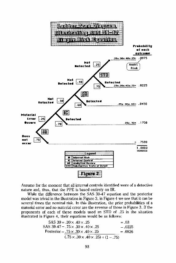
FAR = IR x IC x AR x STD Figure 2 illustrates this modified equation in ladder tree diagram form. The inherent risk that a material error occurs has been set at .25, and its complement, the probability that a material error does not occur, is .75. Note the substantial reduction in FAR (or audit risk as used in SAS 47). If the desired FAR were .03 as used in Figure 1, the result would be the elimination of STD (since IR x IC x AR= .25 x .30 x .40 = .03). Later in the paper, it will be demonstrated that a reduction of STD of this magnitude is not justified with this IR.

Cushing and Loebbecke (1983) use this equation as the focal point of their critique of the risk analysis model. It is here that they make one of a number of critical errors in their paper. They say that this equation is "equivalent to the CICA model" in the CICA Extent of Audit Testing (EAT) Study. Had they continued reading on the page that contained this model (p. 97), they would have learned that this model was not recommended by the Study Group. The EAT Study Group recommended the following model:

FAR= IR x IC x AR x STD (IR x IC x AR x STD) + (1 - IR)

A footnote on page 97 of the EAT Study indicates that further information on the approach can be found in Leslie et al, "Dollar-Unit Sampling," page 296. In fact, this model is the posterior risk model in Leslie et al (1979). The EAT Study Group adopted this model because it "takes the effect of inherent risk more accurately into account." Figure 3 uses the details from Figure 2 and calculates the "posterior risk." In this instance (highly artificial as will be demonstrated later), the difference would appear trivial, although the posterior model would not totally eliminate STD.

It is important to understand the logic applied to Figure 3 to arrive at the posterior risk. It is entirely Bayesian, applied in a discrete (and thus artificial) manner. If the prior probability of error is .25, then, if the auditor proceeds up the steps on the ladder and gets to the end without detecting a material error (of course, it would be necessary for him to investigate the findings of employees responsible for internal control in order to determine if IC detected a material error), he can only be in one of two possible outcomes. Either the material error actually occurred (.25 probability), and IC, AR, and STD failed to detect it, or the material error never occurred in the first place (.75 probability). Since preventive internal controls help prevent the error from occurring in the first place, it is only logical that they be considered together with the inherent risk of error (this will be dealt with in more detail later).

92

Not Detected

Not Detected

Probability of each

outcome

. 2 5 x . 3 0 x . 4 0 x .25= . 0 0 7 5

Audit Risk

Detected . 2 5 x . 3 0 x . 4 0 x . 7 5 = . 0225

. 2 5 x . 3 0 x . 6 0 = .0450

. 2 5 x . 7 0 = .1750

.7500

1.0000

IR Inherent Risk IC Internal Control

AR Analyt ical Review STD Substant ive Tes ts of Detail

Assume for the moment that all internal controls identified were of a detective nature and, thus, that the PPE is based entirely on IR.

While the difference between the SAS 39-47 equation and the posterior model was trivial in the illustration in Figure 3, in Figure 4 we see that it can be several times the nominal risk. In this illustration, the prior probabilities of a material error and no material error are the reverse of those in Figure 3. If the proponents of each of these models used an STD of .25 in the situation illustrated in Figure 4, their equations would be as follows:

SAS 39=.30x.40x.25 =.03 SAS 39-47 =.75 x .30 x .40 x . 25 = .0225 Posterior = .75 x .30 x .40 x .25 = .0826

(.75 x .30 x .40 x .25) + (1 - .75)

93

Ladder Tree Diagram Illustrating SAS 39 - 49 Simple Risk Equation

Probability of each

outcome

However, if they planned to obtain a (final) risk of .03 based on their planning models, their equations would appear as follows:

SAS 39 = .30x.40x.25 =.03 SAS 39-47 = .75 x .30 x .40 x .333 = .03 Posterior = .75 x .30 x .40 x .0859 = .03

(.75 x .30 x .40 x .0859) + (1 - .75)

What would these different values for STD mean in practice? It is useful to compare the difference in sample extents that would result from these STDs. Using dollar-unit sampling (zero expected error case) and setting the SAS 39 sample size equal to " 1 , " we get the following relationship:

94

Ladder Tree Diagram Illustrating Posterior Risk Equation

F i g u r e 3

SAS 39 1.00 SAS 39-47 .79 Posterior 1.77

The most significent conclusion that can be drawn from this comparison is that the formal inclusion of IR in SAS 47 will result in an unjustifiable reduction in STD. Of course, it can be argued that the model in SAS 39 is simply an example and that it is only intended for planning purposes. However, this proposition can be countered with the argument that the model used for planning should be consistent with the model appropriate for evaluation when the audit evidence has been collected. In my opinion, the only appropriate conceptual model for audit evaluation is the posterior risk model (with some

Probability of each

outcome

F i g u r e 4

95

Ladder Tree Diagram Illustrating Risks When IR/PPE Is High

modifications as will be described later) because it relates directly to the auditor's objective and the audit opinion. In order to give a clean opinion, the auditor must be satisfied that there is a reasonably low risk (.03 in this example) that the financial statements do not contain a material error. The two AICPA "simple risk models" address this issue only at the planning stage. If the auditor does not find a material error, the error is not addressed at the evaluation stage, and the audit objective is simply "assumed" to have been achieved. It was for this reason that the CICA EAT Study Group adopted the posterior model. The Study Group was of the view that the auditor's opinion should be based on the evaluation of the risk that the financial statements actually contain a material error, given all of the avidence available to the auditor, and that this model "takes the effect of inherent risk more accurately into account."

Some members of the AICPA Materiality and Audit Risk Task Force were concerned that the inclusion of IR in the risk model would result in a reduction of work because an auditor could always "fall back'' to IR "for more assurance in highly competitive situations." I certainly share the view of some of my fellow Task Force members. However, I believe that auditors must address IR when planning and evaluating an audit (and I believe the judiciary would agree with my belief). Accordingly, it is even more important that the risk model used in practice not deceive the auditor by permitting him to think he is achieving a specific audit risk objective when, in fact, he may be incurring a real risk that is substantially higher.

Numerical Illustrations Table 1 provides a comparison of the risks generated by the three different

models based on the risks for IC, AR, and STD in the previous illustrations (the first three columns). Column 4 contains the risk objective based on the SAS 39 model (.03). Column 5 contains various IR/PPE values from .05 to 1.0, and the two right-hand columns reflect the risks that would be generated by the SAS 47 model and the posterior model. These risks have been computed in the manner described earlier in this paper (examples §4 and §10 relate to Figures 3 and 4).

It should be noted that both risks in the final two columns are less than the SAS 39 risk until the PPE exceeds .50 (actually slightly over .50). Above a PPE of .50, the SAS 47 risk continues to increase until it reaches its maximum of .03 when the PPE is 1.0. It is then equal to the SAS 39 risk, demonstrating in theory, the comment in the footnote to the Appendix of SAS 39 that "the actual risk will ordinarily be less than UR." Clearly, the word "ordinarily" should be interpreted to mean situations where the PPE does not exceed .50. Perhaps this limitation is what the authors of SAS 39 had in mind when it was drafted. I would suggest, however, that this qualification is not being observed in practice.

Note that when the PPE is 1.0, the actual (posterior) risk is also 1.0, as is only logical because a PPE of 1.0 means that the auditor has "perfect" knowledge that a material error exists and, thus cannot believe the results of the audit if the error has not been detected. (Obviously, the auditor rarely has such "perfect" knowledge that a material error exists. Likewise, there rarely is "perfect" knowledge that a material error does not exist—a PPE of 0.)

96

COM

PARI

SON

OF

RISK

S -

SA

S 3

9,

SA

S 47

AN

D P

OST

ERIO

R

SAS

39

SIM

PLE

SAS

47 E

XTEN

DED

LE

SLIE

ET

AL

JOIN

T RI

SK M

ODEL

JO

INT

RISK

MOD

EL

POST

ERIO

R R

ISK

MOD

EL

EX.

INTE

RN

AL: A

NA

LYTI

CA

L SU

BS.

TES

TS

(FOR

PL

ANN

ING

IN

HER

ENT

(FOR

PL

ANN

ING

(F

OR P

LAN

NIN

G A

ND

#

: CON

TROL

R

EVIE

W

OF D

ETAI

L PU

RPOS

ES O

NLY

) RI

SK/P

PE

PURP

OSES

ON

LY)

EVA

LUA

TIO

N)

1 0.

3000

0.

4000

0.

2500

0.

0300

0.

0500

0.

0015

0.

0016

2

0.30

00

0.40

00

0.25

00

0.03

00

0.10

00

0.00

30

0.00

33

3 0.

3000

0.

4000

0.

2500

0.

0300

0.

2000

0.

0060

0.

0074

S4

0.

3000

0.

4000

0.

2500

0.

0300

0.

2500

0.

0075

0.

0099

5

0.30

00

0.40

00

0.25

00

0.03

00

0.30

00

0.00

90

0.01

27

6 0.

3000

0.

4000

0.

2500

0.

0300

0.

4000

0.

0120

0.

0196

7

.0.3

000

0.40

00

0.25

00

0.03

00

0.50

00

0.01

50

0.02

91

8 0.

3000

0.

4000

0.

2500

0.

0300

0.

6000

0.

0180

0.

0431

9

0.30

00

0.40

00

0.25

00

0.03

00

0.70

00

0.02

10

0.06

54

S10

.0.3

000

0.40

00

0.25

00

0.03

00

0.75

00

0.02

25

0.08

26

11

0.30

00

0.40

00

0.25

00

0.03

00

0.80

00

0.02

40

0.10

71

12

0.30

00

0.40

00

0.25

00

0.03

00

0.90

00

0.02

70

0.21

26

13

0.30

00

0.40

00

0.25

00

0.03

00

0.95

00

0.02

85

0.36

31

14

0.30

00

0.40

00

0.25

00

0.03

00

0.98

00

0.02

94

0.59

51

15

0.30

00

0.40

00

0.25

00

0.03

00

0.99

00

0.02

97

0.74

81

16

0.30

00

0.40

00

0.25

00

0.03

00

1.00

00

0.03

00

1.00

00

TAB

LE 1

97

Whereas SAS 39 "conservatively" set IR equal to 1, SAS 47 uses the term "maximum" to "solve" this problem.3 Unfortunately, this change will probably not be noticed by most readers of SAS 47, and it is likely to be obscure to those who do recognize it.

Table 2 contains some comparisons of these three models based on the IC and AR values used in Table 2 of the Appendix to SAS 39. Here, the .05 risk objective used in SAS 39 has also been used. For the first eleven examples, IR/ PPE has been set at .50 (often referred to as the equivalent of a uniform prior). The STD risk for SAS 39 and the posterior model are basically identical. Logically (from an arithmetic point of view), the SAS 47 allowable risk is double the risk of the other two.

COMPARISON OF TESTING RISK LEVELS REQUIRED

SUBSTANTIVE TEST OF DETAILS RISK REQUIRED TO ACHIEVE A .05

SAS 39 ; SAS 47 LESLIE

EX. INHERENT INTERNAL ANALYTICAL "ULTIMATE" AUDIT POSTERIOR # RISK CONTROL REVIEW RISK RISK RISK

1 0.5000 0.1000 1.0000 0.5000 NTR 0.5260 2 0.5000 0.3000 1.0000 0.1667 0 . 3 3 3 3 0.1753 3 0.5000 0.3000 0 . 5 0 0 0 0 . 3 3 3 3 0.6667 0.3510 4 0.5000 0.3000 0.3000 0 . 5 5 5 6 NTR 0.5850 5 0.5000 0.5000 1.0000 0.1000 0.2000 0.1052 6 0 . 5 0 0 0 0.5000 0 . 5 0 0 0 0 . 2 0 0 0 0.4000 0 . 2 1 0 5 7 0.5000 0.5000 0.3000 0 . 3 3 3 3 0.6667 0.3510 8 0.5000 1.0000 1.0000 0.0500 0.1000 0.0526 9 0.5000 1.0000 0.5000 0.1000 0.2000 0.1053 10 0.5000 1.0000 0.3000 0 . 1 6 6 7 0 . 3 3 3 3 0.1753 11 0.5000 1.0000 0.1000 0.5000 NTR 0.5260

12 0 . 2 5 0 0 0.1000 1.0000 0 . 5 0 0 0 NTR NTR 13 0.2500 0.3000 1.0000 0 . 1 6 6 7 0.6667 0.5260 14 0.2500 0.3000 0.5000 0 . 3 3 3 3 NTR NTR 15 0 . 2 5 0 0 0.3000 0.3000 0.5556 NTR NTR 16 0.2500 0.5000 1.0000 0.1000 0.4000 0.3160 17 0.2500 0.5000 0.5000 0.2000 0.8000 0.6320 18 0.2500 0.5000 0.3000 0 . 3 3 3 3 NTR NTR 19 0.2500 1.0000 1.0000 0.0500 0.2000 0.1580 20 0.2500 1.0000 0.5000 0.1000 0.4000 0.3160 21 0.2500 1.0000 0.3000 0.1667 0.6667 0.5260 22 0.2500 1.0000 0.1000 0.5000 NTR NTR

NTR = NO TEST REQUIRED INTERNAL CONTROL AND ANALYTICAL REVIEW FACTORS FROM TABLE 2 , APPENDIX, SAS 39

TABLE 2

98

The bottom eleven examples are based on an IR/PPE set equal to .25 (a favourable prior). In these cases, the SAS 47 allowable STD risk is four times the allowable SAS 39 STD risk. On the other hand, the allowable STD risk for the posterior model is slightly more than three times the SAS 39 allowable STD risk.

Table 3 contains some additional comparisons where the IR/PPE is unfavourable (.75 and .90). These comparisons have been made via the dollar-unit sampling extent that would be used if no errors were expected.* The SAS

* Given these priors an auditor would be foolish to use what is termed a "discovery sample" (designed to accept only when no errors are found). However, it is the most convenient case to use. For sample sizes designed to accept errors without breaching the materiality limit, the differences in extents would be somewhat less.

COMPARISON OF DUS EXTENTS - HIGH PRIOR PROBABILITY OF ERROR

RATIO OF DOLLAR-UNIT SAMPLE SIZES

SAS 47 POSTERIOR POSTERIOR EX. INHERENT INTERNAL ANALYTICAL TO TO TO

# RISK/PPE CONTROL REVIEW SAS 39 SAS 39 SAS 47 •

1 0.7500 0.1000 1.0000 0.5850 2.5121 4.2945 2 0.7500 0.3000 1.0000 0.8394 1.5843 1.8874 3 0.7500 0.3000 0.5000 0.7381 1.9530 2.6458 4 0.7500 0.3000 0.3000 0.5106 2.7812 5.4473 5 0.7500 0.5000 1.0000 0.8751 1.4547 1.6624 6 0.7500 0.5000 0.5000 0.8213 1.6505 2.0098 7 0.7500 0.5000 0.3000 0.7381 1.9530 2.6458 8 0.7500 1.0000 1.0000 0.9040 1.3495 1.4928 9 0.7500 1.0000 0.5000 0.8751 1.4547 1.6624

10 0.7500 1.0000 0.3000 0.8394 1.5843 1.8874 11 0.7500 1.0000 0.1000 0.5850 2.5121 4.2945

12 0.9000 0.1000 1.0000 0.8480 4.0954 4.8295 13 0.9000 0.3000 1.0000 0.9412 2.1975 2.3348 14 0.9000 0.3000 0.5000 0.9041 2.9530 3.2662 15 0.9000 0.3000 0.3000 0.8208 4.6503 5.6659 16 0.9000 0.5000 1.0000 0.9542 1.9318 2.0244 17 0.9000 0.5000 0.5000 0.9345 2.3331 2.4966 18 0.9000 0.5000 0.3000 0.9041 2.9530 3.2662 19 0.9000 1.0000 1.0000 0.9648 1.7162 1.7788 20 0.9000 1.0000 0.5000 0.9542 1.9318 2.0244 21 0.9000 1.0000 0.3000 0.9412 2.1975 2.3348 22 0.9000 1.0000 0.1000 0.8480 4.0954 4.8295

INTERNAL CONTROL AND ANALYTICAL REVIEW FACTORS FROM TABLE 2, APPENDIX, SAS 39

TABLE 3

99

39 sample size has been set equal to " 1 " for these comparisons. In all cases, the SAS 47 sample size is less than the SAS 39 sample size. The sample sizes produced by the posterior model are much larger than both the SAS 39 and SAS 47 sample sizes.

With respect to the reflection of IR in the audit process, these illustrations demonstrate that SAS 47 can actually be a retrogressive step if an appropriate risk model is not employed. It gives too much weight to favourable priors, and it dangerously ignores those that are unfavourable. On the other hand, SAS 39 ignores the priors entirely, resulting in overauditing when they are favourable and underauditing when they are unfavourable. It might be tempting to argue that the situation more than "averages out'' for SAS 39 since far fewer than 50 percent of all audits would have a PPE greater than .50 (and thus overauditing is more frequent than underauditing). Would such a defense be acceptable in court? Would users of financial statements who have suffered losses as a result of inadequate audit extents be happy with such an answer? Losses are certainly not "averaged out'' over all the clients of an auditor when they are discovered.

Prior Probability of Error—Inherent Risk and Preventive Internal Controls

Cushing and Loebbecke (1983) express serious concerns about the independence of the factors in the risk model. As a solution, they suggest (page 29):

A more reasonable approach might be to define inherent risk as conditional upon the quality of the internal control system. Mathematically speaking, this is the correct way to formulate the model. It is also consistent with the frequent audit practice of identifying "special risks" or "sensitive areas" during audit planning. However, neither the AICPA nor CICA model suggests or implies such an approach.

I noted earlier that what they referred to as the CICA model is, in fact, the AICPA post SAS 47 model. I would strongly submit that the CICA model (and, obviously, the Leslie et al model on which it was based) adequately addresses this issue. Leslie et al (1979, p. 307) stated:

Of particular relevance to the auditor is the distinction between preventive controls and detective controls. Preventive controls seek to prevent the occurrence of errors or irregularities—or, more accurately, to reduce their chance of occurrence. Detective controls seek to detect such errors or irregularities as do occur—or, more accurately, to increase their chance of detection. Usually, both types of control are desirable. The need for controls of a preventive nature is less, the greater the inherent insusceptibility to material error. Most auditors assess the prior probabilities of an error occurring in the first place after considering the nature and effectiveness of preventive controls. The Cushing and Loebbecke article leads directly to the conclusion that IR

should be considered "high" if IC is "high." I believe that this is a myth that should be dispelled. An example will illustrate my point:

Consider the inventories of two different types of business. Firm A is a large financial institution that holds billions of dollars worth of marketable securities for its own account and as custodian for customers. Firm B makes steel reinforced concrete supports for expressway construc-

100

tion (minimum weight of two tons). An auditor would be very concerned if Firm A did not have a well designed system of preventive controls (an appropriate class of vault, armed guards, controlled securities cage, segregation of duties relating to the recording and custody functions, a record of certificate numbers, registration of certificates, use of jumbo certificates [for example, where the holding of Ford Motor Company stock had not dropped below 900,000 shares for a considerable period, one share certificate for 900,000 shares would be obtained from the transfer agent rendering the certificate virtually impossible to dispose of if stolen or lost], etc.). We know that if Firm A were to leave these securities sitting on tables in the general office with no such controls, they would disappear rapidly. Firm B, on the other hand, would waste money if it fenced the yard, installed an alarm system, hired armed guards with attack dogs, etc. Many more examples of contrasting situations of this nature can be cited,

and I am sure that practitioners will find that many come to mind rather quickly. Thus, if auditors automatically consider IR to be high when IC is high, they are virtually certain to overaudit in a high proportion of cases. Further, to make recommendations for preventive control improvements when IR is low (and, thus, potential benefits are limited) could cause clients to question an auditor's understanding of the purpose of internal control. Management generally seeks some constant low risk of errors occurring, and its decision on the implementation of preventive controls will be strongly influenced by the inherent risk of error in the first place. K.P. Johnson (1981) made some useful comments on assessing risks that warrant repeating here.

Before a system of internal control can be designed, or an existing system evaluated, management must know something about the kinds of business and transaction risks that exist in its particular organization, assess their significance, and determine which ones cannot be avoided. Only then can controls be designed to reduce the remaining risks to those that are consciously acceptable to management and are at a level that management has consciously determined. Internal controls should not be confused with, or limited to, the accounting system. While an accounting system is a necessary element of a system of internal control, the control system is much larger in scope. A good system of internal control contains elements that have little or no relationship to accounting activities. For example, requirements for advance approval of transactions and restrictions on physical access to assets are examples of internal controls that reduce the risk of errors; they also operate outside of the accounting system. Internal controls are introduced into the accounting system and into other aspects of enterprise operations to prevent errors from occurring in the first place, and to detect them on a timely basis if they do occur. It is important that the inherent risk judgments be made separately for each

financial statement assertion. The illustration above involved the existence assertion. With respect to the valuation assertion, the inherent risk assessment could be just the opposite. For example, the market values for securities are readily available from reputable independent pricing services. On the other hand, the steel reinforced structures could involve very complex pricing since many consist of special high-strength steel rods. The steel is purchased from a German mill in units of 1,000 kilograms, and the purchase invoice is in

101

Deutsche marks. To arrive at a cost, it is necessary to convert steel rod measurements for length and diameter to pounds, and then to kilograms. It is then necessary to apply a price per kilogram based on a conversion of Deutsche marks to dollars with the addition of freight and duty—a far more complex calculation than the pricing of securities based on an independent pricing service. The auditor, therefore, would assess the inherent risk for the valuation assertion as high and would try to identify controls that reduce that risk.

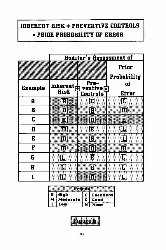
Figure 5 is an illustration of how an auditor could go about making an assessment of the PPE. If he were a "quanto," he would make the assessment in numerical terms by stating a probability. If he were a "judgo," he would make the assessment in nonquantitative terms4 such as high, moderate, or low. In examples A, B, and C, the IR is high, and he would look for preventive controls to mitigate the risk. In example A, the preventive controls are excellent (such as those described for the financial institution above), and he concludes that the PPE is low. In example B, the PICs are good (rather than excellent), and he makes an assessment of the PPE as moderate. In example C, there are no PICs (or any that exist are evaluated as ineffective), and, thus, he assesses the PPE as high. The same logic applies to examples D to I. In examples G and H, it should be noted that there is no apparent payback for identifying PICs. These two examples demonstrate that the auditor is cognizant of the risk of "double counting."* For example, G would be similar to Firm B (in the earlier example) fencing its storage yard, installing an alarm system, hiring armed guards with attack dogs, etc. Any reduction of an already low risk would be so trivial that it would not be sensible to give any credit for it. In example D, only partial credit is given since excellent PICs would not improve the situation beyond a low PPE. The additive illustration in Figure 5 is not intended to imply that the associated probabilities are additive but, rather, that the auditor's knowledge of these two components is additive.

This figure can also illustrate why the auditor must work harder when there is a high PPE. Consider examples A and C. Suppose that in each of these examples the risks for DIC, AR, and STD are identical and neither auditor finds a material error during the audit. Logically, the auditor in example A should be able to sleep well at night because his sample confirmed his prior belief. However, the auditor in example C should have trouble sleeping at night. His sample did not find evidence that supported his prior belief—that a material error more than likely existed. The posterior model would require more evidence (from one or all of DIC, AR, and STD) to be obtained in example C than both of the AICPA models. More evidence is required to obtain a "not guilty" verdict when there is prima facie evidence of a crime than when it is highly likely that a crime was not committed in the first place.

* Cushing and Loebbecke expressed concern over the independence of the component risks. Making the PPE assessment in this manner provides protection against this potential problem.

102

INHERENT RISK + PREVENTIVE CONTROLS = PRIOR PROBABILITY OF ERROR

Auditor's Assessment of

Example Inherent Risk

Preventive [=] Controls

Prior Probability

of Error

103

Figure 5

Have We Now Identified the Theoretically Correct Audit Risk Model?

I have a great subject [statistics] to write upon, but feel keenly my literary incapacity to make it easily intelligible without sacrificing accuracy and thoroughness.

Sir Francis Galton

Unfortunately, we have not. Cushing and Loebbecke (page 27), in criticizing the SAS 47 model (which they mistakenly identified as the CICA model) made some valid observations about discrete models of the type we have been dealing with to this point.*

Models such as this are abstractions of reality. They are used to gain a better understanding of reality and to make reasonably reliable and useful predictions. However, they are always simplified; i.e., all aspects of reality can rarely if ever be accurately incorporated into a model. This simplification is appropriate as long as it is not overdone or done improperly. The measure of this would be whether the model caused the user to misunderstand the reality being represented, or to use the model unwittingly to make unreliable predictions.

After a discussion of these simple joint risk models, Leslie et al (p. 304) described the oversimplification as follows:

The joint risk model discussed is an oversimplification because it assumes that there is only one discrete risk, namely, the risk of a material error. In fact, there should be a continuous distribution of probabilities of occurrence (and detection) of errors aggregating various amounts. . . . The audit can be described as a continuous process. In theory, the auditor

commences this process with a continuous distribution representing the prior probability of error based on his assessment of inherent risk and preventive controls. As each piece of evidence is obtained the auditor revises this distribution. If the evidence is favourable, the peak of the curve will move away from materiality, and the area of the curve beyond materiality will diminish. Conversely, if a piece of evidence is unfavourable, the peak will move toward materiality, and more of the area will be beyond that point. When all procedures have been completed, the final (posterior) distribution is the basis for the opinion given on the financial statements. If the distribution peaks well to the left of materiality with only a small portion in the right tail, an unqualified opinion would be warranted. If the distribution peaks to the right of materiality (most likely error exceeds materiality), a qualified opinion would usually be warranted. If the distribution peaks to the left of materiality but the area to the right of materiality is too large, then the risk would be too high to warrant an unqualified opinion even though a material error would not be likely. The auditor would not have obtained "reasonable assurance" that a material error did not exist.

In the past, the theoretically correct model has been virtually impossible to use in practice. Now, with the increasing use of computerized audit decision

* It should, however, be noted that their concerns are considerably different than mine. Their paper proposes a model that lacks the same reality that causes their criticism of the post SAS 47 model.

104

aids, it is becoming increasingly more feasible. It is not difficult to predict that within the foreseeable future such complex models will be an integral part of the audit. In the process of describing the theoretically correct model, I will avoid the use of calculus and continuous distributions* by chopping up such distributions into smaller pieces for use in an extended discrete posterior risk model that behaves like the "real thing."

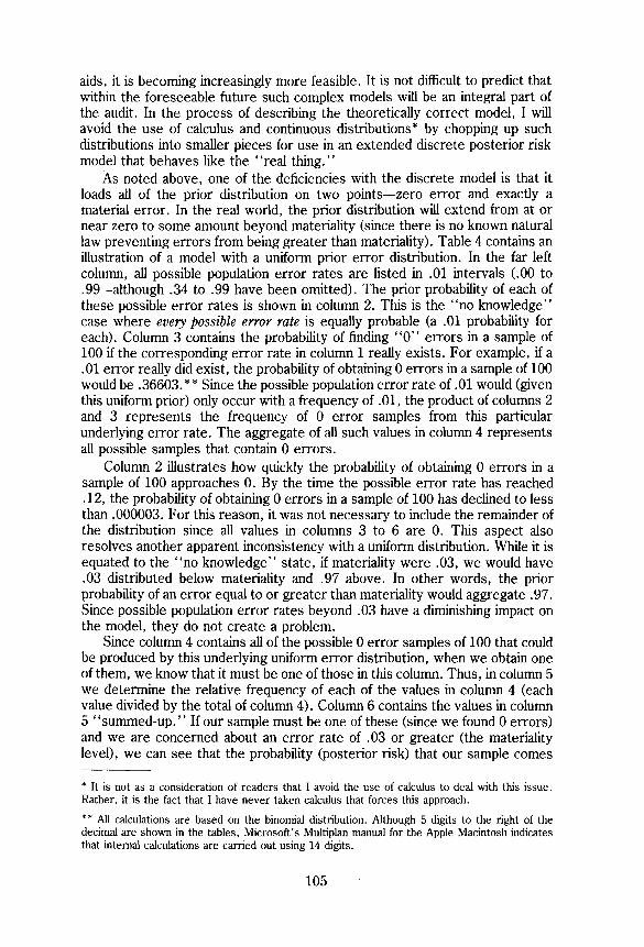
As noted above, one of the deficiencies with the discrete model is that it loads all of the prior distribution on two points—zero error and exactly a material error. In the real world, the prior distribution will extend from at or near zero to some amount beyond materiality (since there is no known natural law preventing errors from being greater than materiality). Table 4 contains an illustration of a model with a uniform prior error distribution. In the far left column, all possible population error rates are listed in .01 intervals (.00 to .99—although .34 to .99 have been omitted). The prior probability of each of these possible error rates is shown in column 2. This is the "no knowledge" case where every possible error rate is equally probable (a .01 probability for each). Column 3 contains the probability of finding "0" errors in a sample of 100 if the corresponding error rate in column 1 really exists. For example, if a .01 error really did exist, the probability of obtaining 0 errors in a sample of 100 would be .36603.** Since the possible population error rate of .01 would (given this uniform prior) only occur with a frequency of .01, the product of columns 2 and 3 represents the frequency of 0 error samples from this particular underlying error rate. The aggregate of all such values in column 4 represents all possible samples that contain 0 errors.

Column 2 illustrates how quickly the probability of obtaining 0 errors in a sample of 100 approaches 0. By the time the possible error rate has reached .12, the probability of obtaining 0 errors in a sample of 100 has declined to less than .000003. For this reason, it was not necessary to include the remainder of the distribution since all values in columns 3 to 6 are 0. This aspect also resolves another apparent inconsistency with a uniform distribution. While it is equated to the "no knowledge" state, if materiality were .03, we would have .03 distributed below materiality and .97 above. In other words, the prior probability of an error equal to or greater than materiality would aggregate .97. Since possible population error rates beyond .03 have a diminishing impact on the model, they do not create a problem.

Since column 4 contains all of the possible 0 error samples of 100 that could be produced by this underlying uniform error distribution, when we obtain one of them, we know that it must be one of those in this column. Thus, in column 5 we determine the relative frequency of each of the values in column 4 (each value divided by the total of column 4). Column 6 contains the values in column 5 "summed-up." If our sample must be one of these (since we found 0 errors) and we are concerned about an error rate of .03 or greater (the materiality level), we can see that the probability (posterior risk) that our sample comes

* It is not as a consideration of readers that I avoid the use of calculus to deal with this issue. Rather, it is the fact that I have never taken calculus that forces this approach.

** All calculations are based on the binomial distribution. Although 5 digits to the right of the decimal are shown in the tables, Microsoft's Multiplan manual for the Apple Macintosh indicates that internal calculations are carried out using 14 digits.

105

EXAMPLE OF POSTERIOR RISK - UNIFORM PRIOR ERROR

Prior Relative Posterior Possible Probability Probability Frequency Risk

Population Of Error Of 0 Error Column 2 Of Prob. ( o f error Error Rate In In Sample X In rate t h a n

Rates Column 1 Of 100 Column 3 Column 4 Column 1)

0.000 0.010 1.00000 0.01000 0.63609 1.00000 0.010 0.010 0.36603 0.00366 0.23283 0.36391 0.020 0.010 0.13262 0.00133 0.08436 0.13109 0.030 0.010 0.04755 0.00048 0.03025 0.04673 0.040 0.010 0.01687 0.00017 0.01073 0.01648 0.050 0.010 0.00592 0.00006 0.00377 0.00575 0.060 0.010 0.00205 0.00002 0.00131 0.00198 0.070 0.010 0.00071 0.00001 0.00045 i 0.00068 0.080 0.010 0.00024 0.00000 0.00015 0.00023 0 .090 0.010 0.00008 0.00000 0.00005 0.00008 0.100 0.010 0.00003 0.00000 0.00002 0.00003 0.110 0.010 0.00001 0.00000 0.00001 i 0.00001 0.120 0.010 0.00000 0.00000 0.00000 0.00000 0.130 0.010 0.00000 0.00000 0.00000 0.00000 0.140 i 0.010 0.00000 0.00000 0.00000 0.00000 0.150 0.010 0.00000 0.00000 0.00000 0.00000 0.160 0.010 0.00000 0.00000 0.00000 0.00000 0.170 0.010 0.00000 0.00000 0.00000 0.00000 0.180 0.010 0.00000 0.00000 0.00000 0.00000 0.190 0.010 0.00000 0.00000 0.00000 0.00000 0.200 0.010 0.00000 0.00000 0.00000 0.00000 0.210 0.010 0.00000 0.00000 0.00000 0.00000 0.220 0.010 0.00000 0.00000 0.00000 0.00000 0.230 0.010 0.00000 0.00000 0.00000 0.00000 0.240 0.010 0.00000 0.00000 0.00000 0.00000 0.250 0.010 0.00000 0.00000 0.00000 0.00000 0.260 0.010 0.00000 0.00000 0.00000 0.00000 0.270 0.010 0.00000 0.00000 0.00000 0.00000 0.280 0.010 0.00000 0.00000 0.00000 0.00000 0.290 0.010 0.00000 0.00000 0.00000 0.00000 0.300 0.010 0.00000 0.00000 0.00000 0.00000 0.310 0.010 0.00000 0.00000 0.00000 0.00000 0.320 i 0.010 0.00000 0.00000 0.00000 0.00000 0.330 0.010 0.00000 0.00000 0.00000 0.00000

TABLE 4

106

from a population with an underlying error rate of .03 or more is .04673. This is virtually identical to the classical (i.e., non-Bayesian) sampling risk for a sample of 100 and a .03 population error rate (which is .04755 as shown in column 3).

If our sample of 100 had contained, say, 1 error, the probability in column 3 would have been computed for 1 error instead of 0 errors. All other calculations would remain the same. We make this calculation for the exact number of errors we find, ignoring all of the other error cases because we know we cannot be in any of them.

Table 5 (in 3 parts) contains a complete example of a uniform prior. In this instance, the possible population error rates have been limited to a narrower range (0 to .099, in 100 increments of .001). This is probably a closer resemblance to a "no knowledge" distribution for an audit (0 to 3.3 times materiality rather than 0 to 33 times materiality). At the .03 possible error rate at the bottom of part 1, it can be seen that the posterior risk of this much error (or more) is still equivalent to the classical sampling risk.

The subsequent posterior risk tables are all based on a sample of 115 to facilitate a comparison with Figures 1 to 4. If a .03 error existed, the probability of a sample of 115 containing 0 errors would also be .03.* Thus, a sample of 115 will yield the same risk as the product of IC, AR, and STD in Figures 1 to 4 (.30 x.40 x .25 = .03).

The illustration at the top of Table 6 represents the 50/50 distribution for a discrete model (the equivalent of the uniform priors in Tables 4 and 5).** At the material error value (.03001), the classical sampling probability and the posterior risk are virtually equal (.03008 and .02920). The SAS 39 model would imply a risk of .03, the SAS 47 model would imply a risk of .015, and the simple discrete posterior model would indicate .0291 (see Table 1). However, if the prior is stacked 50/50 at $1 over and $1 under materiality, the posterior risk rises to virtually .50 as illustrated at the bottom of Table 6. The illustration at the top of Table 7 spreads the .5 portion of the prior below materiality in a level or uniform manner, but stacks the .5 above, right at materiality. In this case, the posterior risk rises to .08347 or almost three times the stated risks for the discrete posterior model and the SAS 39 model. It is almost six times the stated risk for the SAS 47 model. This result is due to the fact that the simple discrete models ignore reality when they stack the priors on 0 errors and a material error. Of course, these last two illustrations are not realistic either.

The illustration at the bottom of Table 7 reflects the circumstances in Figure 3. This condition results in the same posterior risk of .0099. The circumstances in Figure 4 are reflected in the illustration at the top of Table 8, and once more the results are in agreement. But neither of these two illustrations can be considered to represent reality. The illustration at the bottom of Table 8 contains the same prior as the illustration at the top, but in

* Readers should ensure that they do not confuse the two .03 values. One is a risk; the other is the materiality level selected for purposes of the illustration. The fact that they are the same in this illustration is entirely coincidental.

** If $30,000 is the materiality level, does this mean that an amount greater than $30,000 ($30,001 and above) would be material, or does it mean $30,000 and above? To avoid splitting hairs, I have loaded the portion of the distribution applicable to a material error at or above .03001 and the portion applicable to less than a material error at or below .02999.

107

EXAMPLE OF POSTERIOR RISK - LIMITED UNIFORM PRIOR ERROR


Population: Of Error Of 0 Error Column 2 Of Prob. (of error Error Rate In In Sample X In rate x than Rates Column 1 Of 100 Column 3 Column 4 Column 1)

0.000 0.010 1.00000 0.01000 0.09607 1.00000 0.001 0.010 0.90479 0.00905 0.08692 0.90393 0.002 0.010 0.81857 0.00819 0.07864 0.81701 0.003 0.010 0.74048 0.00740 0.07114 0.73837 0.004 0.010 0.66978 0.00670 0.06435 0.66723 0.005 0.010 0.60577 0.00606 0.05820 0.60288 0.006 0.010 0.54782 0.00548 0.05263 0.54469 0.007 0.010 0.49536 0.00495 0.04759 0.49206 0.008 0.010 0.44789 0.00448 0.04303 0.44447 0.009 0.010 0.40492 0.00405 0.03890 0.40144 0.010 0.010 0.36603 0.00366 0.03516 0.36254 0.011 0.010 0.33085 0.00331 0.03178 0.32737 0.012 0.010 0.29902 0.00299 0.02873 0.29559 0.013 0.010 0.27022 0.00270 0.02596 0.26686 0.014 0.010 0.24417 0.00244 0.02346 0.24090 0.015 0.010 0.22061 0.00221 0.02119 0.21745 0.016 0.010 0.19930 0.00199 0.01915 0.19625 0.017 0.010 0.18003 0.00180 0.01730 0.17710 0.018 0.010 0.16261 0.00163 0.01562 0.15981 0.019 0.010 0.14686 0.00147 0.01411 0.14419 0.020 0.010 0.13262 0.00133 0.01274 0.13008 0.021 0.010 0.11975 0.00120 0.01150 0.11734 0.022 0.010 0.10811 0.00108 0.01039 0.10583 0.023 0.010 0.09760 0.00098 0.00938 0.09545 0.024 0.010 0.08810 0.00088 0.00846 0.08607 0.025 0.010 0.07952 0.00080 0.00764 0.07761 0.026 0 . 0 1 0 i 0.07176 0.00072 0.00689 0.06997 0.027 0.010 0.06476 0.00065 0.00622 0.06307 0.028 0.010 0.05843 0.00058 0.00561 0.05685 0.029 0.010 0.05271 0.00053 0.00506 0.05124 0.030 0.010 0.04755 0.00048 0.00457 0.04617 0.031 0.010 0.04289 0.00043 0.00412 0.04161 0.032 0.010 0.03868 0.00039 0.00372 0.03748 0.033 0.010 0.03489 0.00035 0.00335 0.03377

TABLE 5 - PART 1

108

E X A M P L E OF POSTERIOR RISK - LIMITED UNIFORM PRIOR ERROR

0.034 0.010 0.03146 0.00031 0.00302 0.03042 0.035 0.010 0.02836 0.00028 0.00272 0.02739 0.036 0.010 0.02557 0.00026 0.00246 0.02467 0.037 0.010 0.02305 0.00023 0.00221 0.02221 0.038 0.010 0.02077 0.00021 0.00200 0.02000 0.039 0.010 0.01872 0.00019 0.00180 0.01800 0.040 0.010 0.01687 0.00017 0.00162 0.01621 0.041 0.010 0.01520 0.00015 0.00146 0.01458 0.042 0.010 0.01369 0.00014 0.00132 0.01312 0.043 0.010 0.01234 0.00012 0.00119 i 0.01181 0.044 0.010 0.01111 0.00011 0.00107 i 0.01062 0.045 0.010 0.01001 0.00010 0.00096 0.00956 0.046 0.010 0.00901 0.00009 0.00087 0.00859 0.047 0.010 0.00812 0.00008 0.00078 0.00773 0.048 0.010 0.00731 0.00007 0.00070 0.00695 0.049 0.010 0.00658 0.00007 0.00063 0.00625 0.050 0.010 0.00592 0.00006 0.00057 0.00562 0.051 0.010 0.00533 0.00005 0.00051 0 .00505 0.052 0.010 0.00480 0.00005 0.00046 0.00453 0.053 0.010 i 0.00432 0.00004 0.00041 i 0.00407 0.054 0.010 0.00388 0.00004 0.00037 0.00366 0.055 0.010 0.00349 0.00003 0.00034 0.00329 0.056 0.010 0.00314 0.00003 0.00030 0.00295 0.057 0.010 0.00283 0.00003 0.00027 0.00265 0.058 0.010 0.00254 0.00003 0.00024 0.00238 0.059 0.010 0.00229 i 0.00002 0.00022 0.00213 0.060 0.010 0.00205 0.00002 0.00020 i 0.00191 0.061 0.010 0.00185 0.00002 0.00018 0.00172 0.062 0.010 0.00166 0.00002 0.00016 0.00154 0.063 0.010 i 0.00149 0.00001 0.00014 0.00138 0.064 0.010 0.00134 0.00001 0.00013 0.00124 0.065 0.010 0.00121 0.00001 0.00012 i 0.00111 0.066 0.010 0.00108 0.00001 0.00010 0.00099 0.067 0.010 0.00097 0.00001 0.00009 0.00089 0.068 0.010 0.00087 0.00001 0.00008 0.00079 0.069 0.010 0.00079 0.00001 0.00008 0.00071 0.070 0.010 0.00071 0.00001 0.00007 0.00063 0.071 0.010 0.00063 0.00001 0.00006 0.00057 0.072 0.010 0.00057 0.00001 0 .00005 i 0.00051 0.073 0.010 0.00051 0.00001 0 .00005 i 0.00045

T A B L E 5 - PART 2

109

E X A M P L E OF POSTERIOR RISK - LIMITED UNIFORM PRIOR ERROR

0 . 0 7 4 0.010 0 . 0 0 0 4 6 0 . 0 0 0 0 0 0.00004 0 . 0 0 0 4 0

0 . 0 7 5 0.010 0.00041 0 . 0 0 0 0 0 0.00004 0 . 0 0 0 3 6

0 . 0 7 6 0.010 0.00037 0 . 0 0 0 0 0 0 . 0 0 0 0 4 0 . 0 0 0 3 2

0 . 0 7 7 0.010 0 . 0 0 0 3 3 0.00000 0.00003 0 . 0 0 0 2 8

0 . 0 7 8 0.010 0.00030 0.00000 0.00003 0 . 0 0 0 2 5

0.079 0.010 0.00027 0.00000 0.00003 0.00022

0 . 0 8 0 0 . 0 1 0 0 . 0 0 0 2 4 0 . 0 0 0 0 0 0.00002 0.00020

0.081 0 . 0 1 0 0 . 0 0 0 2 1 0.00000 0 . 0 0 0 0 2 0 . 0 0 0 1 7

0 . 0 8 2 0.010 0 . 0 0 0 1 9 0.00000 0.00002 0 . 0 0 0 1 5

0 . 0 8 3 0.010 0 . 0 0 0 1 7 0.00000 0.00002 0 . 0 0 0 1 3

0 . 0 8 4 0.010 0 . 0 0 0 1 5 0.00000 0.00001 0 . 0 0 0 1 2

0 . 0 8 5 0.010 0.00014 0 . 0 0 0 0 0 0 . 0 0 0 0 1 0 . 0 0 0 1 0

0 . 0 8 6 0.010 0.00012 0.00000 0.00001 0 . 0 0 0 0 9

0 . 0 8 7 0.010 0.00011 0 . 0 0 0 0 0 0.00001 0 . 0 0 0 0 8

0 . 0 8 8 0.010 0.00010 0.00000 0.00001 0 . 0 0 0 0 7

0 . 0 8 9 0.010 0 . 0 0 0 0 9 0.00000 0.00001 0 . 0 0 0 0 6

0.090 0.010 0.00008 0.00000 0.00001 0 . 0 0 0 0 5

0.091 0.010 0.00007 0.00000 0.00001 0 . 0 0 0 0 4

0 . 0 9 2 0.010 0 . 0 0 0 0 6 0.00000 0.00001 0 . 0 0 0 0 3

0 . 0 9 3 0.010 0.00006 0.00000 0.00001 0 . 0 0 0 0 3

0 . 0 9 4 0.010 0 . 0 0 0 0 5 0.00000 0 . 0 0 0 0 0 0 . 0 0 0 0 2

0 . 0 9 5 0.010 0 . 0 0 0 0 5 0 . 0 0 0 0 0 0.00000 0 . 0 0 0 0 2

0.096 0.010 0.00004 0.00000 0 . 0 0 0 0 0 0.00001

0 . 0 9 7 0.010 0.00004 0 . 0 0 0 0 0 0.00000 0.00001

0 . 0 9 8 0.010 0 . 0 0 0 0 3 0 . 0 0 0 0 0 0.00000 0.00001

0 . 0 9 9 0.010 0.00003 0.00000 0.00000 0 . 0 0 0 0 0

1.000 1 0 . 4 0 9 0 7 0 . 1 0 4 0 9 1 . 0 0 0 0 0

T A B L E 5 - PART 3

110

POSTERIOR RISK - 50/50 PRIOR [STACKED ON ZERO AND MATERIALITY]


Population Of Error Of 0 Error Column 2 Of Prob. (of error Error Rate In In Sample X In rate than Rates Column 1 Of 115 Column 3 Column 4 Column 1)

0.00000 0.50000 1.00000 0.50000 0.97080 1.00000 0.03001 0.50000 0.03008 0.01504 0.02920 0.02920

POSTERIOR RISK - 50/50 PRIOR [STACKED AT MATERIALITY]



0.02999 0.50000 0.03015 0.01507 0.50059 1.00000 0.03001 0.50000 0.03008 6.01504 0.49941 0.49941

TABLE 6

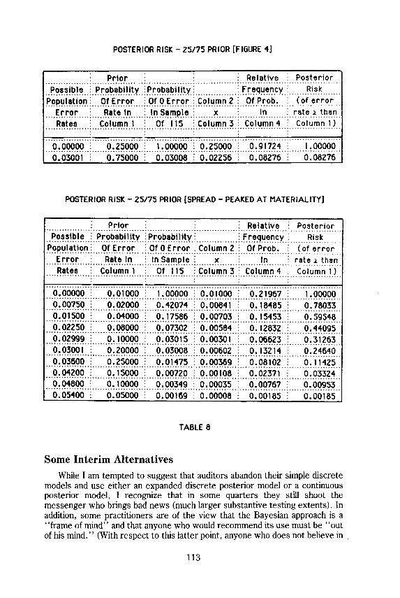
this instance the spread is somewhat realistic (0 to .054, peaking at materiality). This produces a posterior risk of .24640 in comparison with the simple posterior risk of .08276, the SAS 39 risk of .03, and the SAS 47 risk of .0225 (see example §10 in Table 1).

The illustration at the top of Table 9 spreads the 75/25 prior in a similar manner (0 and .04 peaking at materiality). Here we see a true posterior risk of .04301 in comparison with the simple posterior risk of .0099, the SAS 39 risk of .03, and the SAS 47 risk of .0075 (see example §4 in Table 1). The illustration at the bottom of Table 9 spreads the 75/25 prior again but with a lower peak (0 to .05, peaking at .015, which is 50 percent of materiality). The true posterior risk dropped to .01693, and, of course, the three simple risk model results do not change.

We have seen that the simplistic risk models can significantly understate the auditor's risk when he is giving a clean opinion. The SAS 39 model totally ignores IR/PPE. The SAS 47 model gives too much credit to inherent risk

111

POSTERIOR RISK - 50/50 PRIOR [LEVEL BELOW MATERIALITY]


Population Of Error Of 0 Error Column 2 Of Prob. (of error Error Rate In In Sample X In rate than Rates Column 1 of 115 Column 3 Column 4 Column 1)

0.00000 0.05000 1.00000 0.05000 0.27754 1.00000 0.00300 0.05000 0.70785 0.03539 0.19645 0.72246 0.00600 0.05000 0.50053 0.02503 0.13892 0.52601 0.00900 0.05000 0.35357 0.01768 0.09813 0.38709 0.01200 0.05000 0.24949 0.01247 0.06924 0.28897 0.01500 0.05000 0.17586 0.00879 0.04881 0.21973 0.01800 0.05000 0.12383 0.00619 0.03437 0.17092 0.02100 0.05000 0.08710 0.00435 0.02417 0.13655 0.02400 0.05000 0.06120 0.00306 0.01698 0.11238 0.02700 0.05000 0.04295 0.00215 0.01192 0.09539 0.03001 0.50000 0.03008 0.01504 0.08347 0.08347

POSTERIOR RISK - 75/25 PRIOR [FIGURE 3]



0.00000 0.75000 1.00000 0.75000 0.99007 1.00000 0.03001 0.25000 0.03008 0.00752 0.00993 0.00993

TABLE 7

when it is favourable, and when it is unfavourable the impact is in the wrong direction. The simple posterior model suffers when the PPE is stacked on zero and materiality and the portion below materiality should be spread in what would amount to an unfavourable pattern. Since none of the simple models recognize the possibility of the actual underlying error being well in excess of materiality, it is not clear how the auditor would evaluate the results when a single material error is actually discovered. If a significant portion of the prior distribution actually extended beyond twice materiality, he could well be ignoring undetected error that still exceeded materiality.

112

POSTERIOR RISK - 25/75 PRIOR [FIGURE 4]


Population Of Error Of 0 Error Column 2 Of Prob. (of error Error Rate In In Sample X In rate x than Rates Column 1 Of 115 Column 3 Column 4 Column 1)

0.00000 0.25000 1.00000 0.25000 0.91724 1.00000 0.03001 0.75000 0.03008 0.02256 0.08276 0.08276

POSTERIOR RISK - 25/75 PRIOR [SPREAD - PEAKED AT MATERIALITY]


Population Of Error Of 0 Error Column 2 Of Prob. (of error Error Rate In In Sample X In rate x than Rates Column 1 Of 115 Column 3 Column 4 Column 1)

0.00000 0.01000 1.00000 0.01000 0.21967 i 1.00000 0.00750 0.02000 0.42074 0.00841 0.18485 0.78033 0.01500 0.04000 0.17586 0.00703 0.15453 0.59548 0.02250 0.08000 0.07302 0.00584 0.12832 0.44095 0.02999 0.10000 0.03015 0.00301 0.06623 0.31263 0.03001 0.20000 0.03008 0.00602 0.13214 0.24640 0.03600 0.25000 0.01475 0.00369 0.08102 i 0.11425 0.04200 0.15000 0.00720 0.00108 0.02371 0.03324 0.04800 0.10000 0.00349 0.00035 0.00767 0.00953 0.05400 0.05000 0.00169 0.00008 0.00185 0.00185

TABLE 8

Some Interim Alternatives While I am tempted to suggest that auditors abandon their simple discrete

models and use either an expanded discrete posterior model or a continuous posterior model, I recognize that in some quarters they still shoot the messenger who brings bad news (much larger substantive testing extents). In addition, some practitioners are of the view that the Bayesian approach is a "frame of mind'' and that anyone who would recommend its use must be "out of his mind." (With respect to this latter point, anyone who does not believe in

113

POSTERIOR RISK - 75/25 PRIOR [SPREAD - PEAKED AT MATERIALITY]



0.00000 0.02000 1.00000 0.02000 0.15745 1.00000 0.00500 0.05000 0.56189 0.02809 0.22117 0.84255 0.01000 0.08000 0.31481 0.02518 0.19826 0.62138 0.01500 0.10000 0.17586 0.01759 0.13844 0.42312 0.02000 0.15000 0.09795 0.01469 0.11566 0.28468 0.02500 0.22500 0.05439 0.01224 0.09634 0.16902 0.02999 0.12500 0.03015 0.00377 0.02967 0.07268 0.03001 0.12500 0.03008 0.00376 0.02960 0.04301 0.03500 0.07500 0.01662 0.00125 0.00981 0.01341 0.04000 0.05000 0.00915 0.00046 0.00360 0.00360

POSTERIOR RISK - 75/25 PRIOR [SPREAD - PEAKED AT 0.5 MATERIALITY]



0.00000 0.05000 1.00000 0.05000 0.26618 1.00000 0.00500 0.07500 0.56189 0.04214 0.22435 0.73382 0.01000 0.12500 0.31481 0.03935 0.20949 0.50947 0.01500 0.17500 0.17586 0.03078 0.16384 0.29998 0.02000 0.15000 0.09795 0.01469 0.07822 0.13614 0.02500 0.10000 0.05439 0.00544 0.02896 0.05792 0.02999 0.07500 0.03015 0.00226 0.01204 0.02897 0.03001 0.02500 0.03008 0.00075 0.00400 0.01693 0.03500 0.09000 0.01662 0.00150 0.00796 0.01293 0.04000 0.07000 0.00915 0.00064 0.00341 0.00496 0.04500 0.05000 0.00502 0.00025 0.00134 0.00155 0.05000 0.01500 0.00274 0.00004 0.00022 0.00022

TABLE 9

114

the Bayesian approach should be doing a constant amount of work on all audits regardless of how low or high inherent risk is assessed. I believe that the competitive environment will adequately deal with this problem when the PPE is favourable. As well, the increase in litigation resulting from significant audit failures will, no doubt, cause auditors to do more work when the PPE is unfavourable.)

Cushing and Loebbecke (1983) suggest that the SAS 39 model not be used "when the auditor believes that the likelihood of material error is high." They suggest that some other model (unspecified) would be more appropriate in such circumstances. Given the foregoing illustrations of the failure of the SAS 39 and 47 models when the prior risk of error is high, it is not difficult to agree with this suggestion. But the question remains as to what alternative the auditor has at the present time. He could throw up his hands in frustration and revert to "good old gut feel" until a reliable computerized Bayesian planning and evaluation model becomes available.* This would certainly not be a very progressive step.

One interim solution might be to modify the discrete posterior model in an attempt to correct the deficiency resulting from the stacking of the prior probability of error on only two points. One approach that I am in the process of investigating involves using some fraction of materiality (such as ½ or 2/3) as the cut-off for the portion of the prior distribution that would be stacked on zero. The balance would be placed on materiality, resulting in a reduction of the allowable STD risk and, thus, requiring a larger sample. Although too early to judge, this approach might provide a workable procedure.

Another interim solution would be to use an extended discrete model with the auditor actually specifying the prior distribution over reasonably short intervals (such as 10hs or 5ths of materiality). IC and AR could be integrated into the model by using the equivalent prior sample concept.5 This procedure involves inputting the values for IC and AR in terras of a sample size and a specific number of errors (this is very convenient because the parameters for the βeta distribution can be described in these terms and the βeta distribution can model audit priors in a very "realistic" manner). Such a model could be used for planning and evaluation, and it could be programmed for use on a micro-computer at a reasonable cost.

When an auditor believes that a material error does not exist (low PPE), he collects evidence to support this belief. When he believes that a material error does exist (high PPE), he should attempt to prove that case rather than cross his fingers and hope he can prove that the situation is actually acceptable (this is why the posterior risk model requires a much larger substantive sample if the auditor wishes to "accept" when the PPE is high). The auditor can use the posterior risk model in another manner that would address the concerns expressed by Cushing and Loebbecke and also reduce the size of the substantive sample. This approach would require the auditor to change his outlook when the PPE is high. Instead of accepting the underlying population as

* A quasi-Bayesian model purported to contain all of the desirable features of an audit risk model was recently described by McCray (1984). While this model may have some promise, it has not yet been subjected to a thorough analysis by the accounting and statistical professions. In addition, it has not been tested in a live audit environment.

115

being free of material error when he failed to detect it, he would search further because the result would be inconsistent with his expectation. Thus, he could start with a reduced sample extent and enlarge it if he failed to identify the expected error condition. The most common decision rule used in practice at the present time is just the opposite—start with a small sample and enlarge it only if errors are found.

Researchers in practice and academe must be cognizant of the competitive environment. Understandably, client-handling partners of accounting firms will exhibit resistance to changes in the audit risk model if the result is more work. If they could be assured that their competitors were using the same model and achieving the same audit objective, I feel certain that they would not resist what we might all agree are "advances in theory and practice." However, we know that, in the "real world," even the simple models that we criticize are used by only a small minority of practitioners.* An impartial observer might be of the view that we are criticizing the Model T because more advanced models are available when, in fact, our profession is still in the horse and buggy era.

Some Related Issues Even if we were to obtain complete agreement on the appropriate audit risk

model, it would mean little if we could not achieve some degree of uniformity in materiality judgments. Audit risk by itself has absolutely no meaning. It can only be quantified and used in a model when it is related to a specified level of materiality.** In a forthcoming CICA Audit Research Study,6 I have recommended that the profession solve this problem by providing users of financial statements with the level(s) of materiality used in the audit.

Cushing and Loebbecke raised the issue of the aggregation of evidence throughout the audit and lamented the fact that "none of the sources cited in the literature review indicate how the model could be expanded to address the aggregation problem." Once again, they did not look very carefully at the literature they cited since Leslie et al (1979) described a methodology*** for aggregation that is consistent with paragraphs 27 to 32 of SAS 47. I believe that in the very near future this method of aggregation will be attacked in the literature as being without logic, statistical validity, or any other redeeming qualities. In this respect, one is reminded of the mid 1970s when almost everyone was attacking the validity of the Stringer bound. Several researchers recommended alternate bounds that generated much higher upper error limits. Now, of course, all of the literature in this area attacks the Stringer bound as being too inefficient because it is so conservative. A look into my crystal ball suggests that history is about to repeat itself.

* This contention will be illustrated in a forthcoming AICPA Audit Research Monograph by Carl Warren. The basis of this monograph will be the 690 questionnaires submitted by 60 accounting firms as part of the Materiality and Audit Risk Task-force project.

** Readers may have noticed that the final title of SAS 47 reversed the order of "risk" and "materiality" set out in the title of the Exposure Draft. This was the result of the mistaken belief of several members of the ASB that risk is determined before materiality and then used to determine the amount that is material.

*** This method of aggregation, or a variation thereof, is used by Clarkson Gordon, Deloitte Haskins & Sells and several other firms.

116

The Role of Statistical Sampling in Compliance Testing

"If there's no meaning in it," said the King, "that saves a world of trouble, you know, as we needn't try to find any.''

C.L. Dodgson

The debate over the role of statistical sampling in auditing has spanned several decades. One segment of the profession holds the view that statistical sampling has no place in auditing since it results in a reduction in the use of judgment by the auditor. The other segment is of the view that without the use of quantitative methods the auditor has no reasonable method by which to determine testing extents. This latter segment also believes that the use of statistical sampling enhances the use of judgment in the audit process. Members of these two segments are now commonly referred to as "judgos" and "quantos," respectively. I make no attempt to hide the fact that I am a member of the "quanto" segment.

Earlier in this paper, internal controls were identified as being either preventive or detective, and preventive internal controls were considered together with inherent risk in order to determine the prior probability of error. The preventive and detective distinctions are described in both the AICPA "Statements on Auditing Standards" and the CICA "Handbook." The latter includes the following description in paragraph 5205.13: Internal controls may be characterized as preventive or detective. Preventive controls are those which prevent, or minimize the chance of occurrence of, fraud and error. Detective controls do not prevent fraud and error but rather detect them, or maximize the chance of their detection, so that corrective action may be promptly taken. The known existence of detective controls may have a deterrent effect, and be preventive in that sense. It is reasonable to classify a detective control as a preventive control provided that detection will result in the recovery of the particular asset that would otherwise be lost to the entity. Prompt recognition (recording) of a loss by the entity would not qualify the control as one with preventive value. As an example, consider the earlier case of a large financial institution that holds large quantities of securities. If this institution could detect missing securities promptly and recover them, this control feature would serve as a preventive control since a dishonest (or potentially dishonest) employee would be reluctant to steal certificates if negotiating them exposed him to a high probability of being caught. On the other hand, if the institution could detect missing certificates promptly but do little to recover them, the control would be considered entirely detective since it would have no deterrent value.

Certain types of control will be clearly preventive or detective in nature while others may be difficult to classify. In this respect, it is important to develop a decision rule for audit staff in order to avoid "classifications of convenience."

Objectives of Compliance Testing In order to employ statistical sampling in compliance testing, the auditor

must first establish the objective of his compliance tests. SAS Au § 320.59 describes the purpose of compliance tests as follows:

117

The purpose of compliance tests is to provide reasonable assurance that the accounting control procedures are being applied as prescribed. Such tests are necessary if the prescribed procedures are to be relied on in determining the nature, timing, or extent of substantive tests of particular classes of transactions or balances, as discussed later . . .

Other than the reference to "reasonable assurance," the above passage provides no guidance as to "how much compliance testing is enough." Of course, reasonable assurance (the complement of risk) must be related to "something" if it is to have any meaning. The "something" is described in paragraph 31 of SAS 39 (Au § 320.31) as '"the maximum rate of deviations from prescribed control procedures that would support his planned reliance." The subsequent discussion in paragraphs 32 to 42 of SAS 39 has, through the use of examples, established the internationally known and (ab)used "5 & 5 gets ya 60" syndrome. This magic "60" is without a doubt the most commonly employed compliance testing extent in the world. If one is prepared to accept this number,* all of the problems related to compliance testing extents quickly vanish.

Even though this approach would appear to have the blessing of a substantial portion of the profession (silence implies acceptance), it should not go unchallenged. SAS Au § 320.68 states:

The auditor's evaluation of accounting control with reference to each significant class of transactions and related assets should be a conclusion about whether the prescribed procedures and compliance therewith are satisfactory for his purpose. The procedures and compliance should be considered satisfactory if the auditor's review and tests disclose no condition he believes to be a material weakness for his purpose. In this context, a material weakness is a condition in which the specific control procedures or the degree of compliance with them do not reduce to a relatively low level the risk that errors or irregularities in amounts that would be material in relation to the financial statements being audited may occur and not be detected within a timely period by employees in the normal course of performing their assigned functions. (emphasis added)

It is difficult, if not impossible, to determine how the magic number "60" can meet the materiality criterion for every audit engagement.

The following illustration demonstrates the variability in compliance testing payback when this approach is used. These calculations use the SAS 39 model (they ignore inherent risk for simplicity). AR is not effective and has been set equal to 1. In these cases, when the auditor takes his compliance sample of 60 and finds no deviations, he subjectively determines that the IC risk is .25, and, using his risk equation, he increases his allowable sampling risk from a βeta of .05 to a βeta of .20. Columns (4) and (5) contain the DUS extents for each of the βeta risks based on the assumption that no errors will be found throughout the entire audit. In some instances, there is a positive payback, and in others it is negative. It can be seen that the payback is highly variable. But, suppose some of these populations are a part of the same audit engagement. Population 2 is the western accounts receivable supervised by the credit office in Los

* I suspect that Charles Dodgson would consider acceptance of a magic number of this nature as blind faith.

118

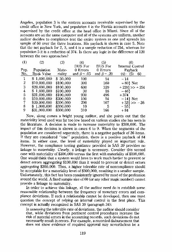
Angeles, population 3 is the eastern accounts receivable supervised by the credit office in New York, and population 4 is the Florida accounts receivable supervised by the credit office at the head office in Miami. Since all of the accounts are on the same computer and all of the systems are uniform, another auditor decides to compliance test the entire system as one and spreads his sample of 60 over the three locations. His payback is shown in case 5. Note that the net payback for 2, 3, and 4 is a sample reduction of 254, whereas for population 5 it is a reduction of 374. Is there any logic in the difference of 120 between the two approaches?

(1) (2) (3) (4) (5) (6) DUS For DUS For Internal Control

Pop. No.

Population Book Value

Materiality

0 Errors and β= .05

0 Errors and β = .20

Payback (4)-(5)-60

1 $ 1,000,000 $ 30,000 100 54 -14 2 $10,000,000 $100,000 300 160 + 80} Net 3 $20,000,000 $100,000 600 320 + 2 2 0 } » + 254 4 $ 1,000,000 $100,000 30 16 -46} 5 $31,000,000 $100,000 930 496 + 374 6 $10,000,000 $300,000 100 54 -14} Net 7 $20,000,000 $300,000 200 107 + 33} » - 36 8 $ 1,000,000 $300,000 10 5 -55} 9 $31,000,000 $300,000 310 166 + 84

Now, along comes a bright young auditor, and she points out that the materiality level used was far too low based on various studies she has seen in the literature. A decision is made to increase materiality to $300,000. The impact of this decision is shown in cases 6 to 9. When the segments of the population are considered separately, there is a negative payback of 36 items. If they are considered "one" population, there is a positive payback of 84 items. In either case, the level of materiality played an important role. However, the compliance testing guidance provided in SAS 39 provides no linkage to materiality. Clearly, a linkage is necessary. Consider this second case with materiality of $300,000 versus the first with materiality of $100,000. One would think that a system would have to work much harder to prevent or detect errors aggregating $100,000 than it would to prevent or detect errors aggregating $300,000. Thus, a higher tolerable rate of noncompliance should be acceptable for a materiality level of $300,000, resulting in a smaller sample. Unfortunately, this fact has been consistently ignored by most of the profession around the world. A fixed sample size of 60 (or any other magic number) cannot provide a linkage to materiality.

In order to achieve this linkage, all the auditor need do is establish some reasonable relationship between the frequency of monetary errors and compliance deviations. If such a relationship cannot be developed, then one must question the concept of relying on internal control in the first place. This concept is actually recognized in SAS 39 (paragraph 34):

In assessing the tolerable rate of deviations, the auditor should consider that, while deviations from pertinent control procedures increase the risk of material errors in the accounting records, such deviations do not necessarily result in errors. For example, a recorded disbursement that does not show evidence of required approval may nevertheless be a

119

transaction that is properly authorized and recorded. Deviations would result in errors in the accounting records only if the deviations and the errors occurred on the same transactions. Deviations from pertinent control procedures at a given rate ordinarily would be expected to result in errors at a lower rate. As many researchers are aware, my associates and I have been expounding

this approach for many years. When we first contemplated using the "5 & 5" fixed sample approach, our associate, Albert Teitlebaum of McGill University, pointed out the lack of logic and statistical consistency. It was his objective view from the sidelines, uncontaminated by the audit literature of the time (SAP 54), that forced us to see the illogical aspects of not relating the extent of compliance testing to materiality. In addition, whenever we attempted to incorporate the value for IC in a risk model, we found that it had to have a relationship to materiality in order to make any sense. The result was the "smoke/fire" methodology that we have described in two books and several papers.7 I hope that participants in this Symposium will focus some of their attention on this issue.

Comparison of Value-Oriented and Neutral Sampling Methods for Compliance Tests

The decision on the objective of compliance testing will impact the auditor's decision on method of sampling and, therefore, the method of selection. If the auditor subscribes to the magic number "60," he will more than likely use a neutral sampling method (all physical units will be given the same chance of selection—physical unit attribute sampling). A decision to relate compliance testing to materiality will generally result in the use of a value-oriented sampling method (DUS, CMA, PPS). The following is an example taken from the forthcoming CICA Audit Research Study on Materiality and from Leslie (1977). The sample of 257 is based on using a βeta risk of .20 and a three times multiple of materiality (see Leslie et al (1979) page 150). The sample of 95 is the magic number "60" expanded to allow acceptance of one compliance deviation without rejecting reliance on IC (consistent with the 257 calculation).

Although the distribution in this illustration is hypothetical, it follows the shape of those found in actual accounting populations. This illustration demonstrates the stark contrast between the selection methods and, perhaps, the importance of using value-oriented selection (where the maximum possible error in an item is related to its book value) regardless of the philosophy used to determine the sample size.

In a number of research experiments carried out by the writer and others, groups of auditors have been requested to select samples from populations on a "judgmental representative" basis. Analysis of these samples revealed that the average judgmental allocation is very close to the V-O (DUS) average and in no way even resembles the neutral allocation. This is the reason why many auditors prefer to use judgmental value-oriented selection rather than physical-unit attributes sampling in cases where they feel the cost of selecting a rigorous value-oriented probability sample (DUS) is not warranted by the added objectivity. When one envisages an auditor describing these two different approaches to an audit committee (or a judge), it is difficult to visualize any

120

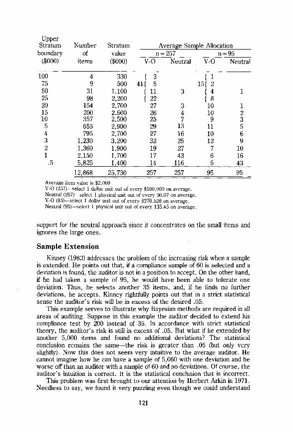
Upper Stratum Number Stratum Average Sample Allocation

boundary ($000)

of items

value ($000)

n = 257 n = 95 boundary ($000)

of items

value ($000) V-0 Neutral V-0 Neutral

100 4 330 [ 3 { 1 75 9 500 41 { 5 15{ 2 50 31 1,100 { 11 3 { 4 1 25 98 2,200 { 22 { 8 20 154 2,700 27 3 10 1 15 200 2,600 26 4 10 2 10 357 2,500 25 7 9 3 5 655 2,900 29 13 11 5 4 795 2,700 27 16 10 6 3 1,230 3,200 32 25 12 9 2 1,360 1,900 19 27 7 10 1 2,150 1,700 17 43 6 16 .5 5,825 1,400 14 116 5 43

12,868 25,730 257 257 95 95 Average item value is $2,000 V-O (257)—select 1 dollar unit out of every $100,000 on average. Neutral (257)—select 1 physical unit out of every 50.07 on average. V-O (95)—select 1 dollar unit out of every $270,526 on average. Neutral (95)—select 1 physical unit out of every 135.45 on average.

support for the neutral approach since it concentrates on the small items and ignores the large ones.

Sample Extension Kinney (1983) addresses the problem of the increasing risk when a sample

is extended. He points out that, if a compliance sample of 60 is selected and a deviation is found, the auditor is not in a position to accept. On the other hand, if he had taken a sample of 95, he would have been able to tolerate one deviation. Thus, he selects another 35 items, and, if he finds no further deviations, he accepts. Kinney rightfully points out that in a strict statistical sense the auditor's risk will be in excess of the desired .05.

This example serves to illustrate why Bayesian methods are required in all areas of auditing. Suppose in this example the auditor decided to extend his compliance test by 200 instead of 35. In accordance with strict statistical theory, the auditor's risk is still in excess of .05. But what if he extended by another 5,000 items and found no additional deviations? The statistical conclusion remains the same—-the risk is greater than .05 (but only very slightly). Now this does not seem very intuitive to the average auditor. He cannot imagine how he can have a sample of 5,060 with one deviation and be worse off than an auditor with a sample of 60 and no deviations. Of course, the auditor's intuition is correct. It is the statistical conclusion that is incorrect.

This problem was first brought to our attention by Herbert Arkin in 1971. Needless to say, we found it very puzzling even though we could understand

121

the strict statistical conclusion. As reported by Teitlebaum (1973), the solution to this problem can be found in Bayesian analysis. For example, if a prior distribution of compliance deviation rates in a population is established (subjectively, of course—and it should be favourable or the auditor has no business considering reliance on IC) and then combined with the results of a compliance sample of 60 containing one deviation, a certain posterior distribution is produced. If this posterior distribution is then used as the prior distribution and combined with a deviation free sample of 35, the posterior distribution produced is identical to the posterior distribution produced by using the original prior and a sample of 95 with one compliance deviation.

Thus, the auditor who employs Bayesian methods can ignore the issue of increasing risk when extending his samples. If his priors are favourable, his results will be acceptable. If his priors are unfavourable, deviation or error free results may not even be acceptable. This posture contrasts to that of the non-Bayesian who will only react to sample results—with no recognition given to his prior beliefs.

Much more extensive research in Bayesian methods and their application to auditing would be desirable. They are applicable to all areas of the attest audit. While prior probability distributions are subjective (and usually somewhat fuzzy) and cannot be "verified," they do and should reflect what the auditor actually believes. If he is prepared to "fudge" his priors in order to do less work, he knows when he concludes his audit that he really does not have the reasonable assurance he set out to obtain. He is then forced to live with his conscience.

Is Compliance Testing Really Necessary in Order to Place Reliance on Internal Control?

Based on auditing standards in Canada and the U.S., the answer would seem to be an obvious "yes." Perhaps it is time, however, to take another look at this requirement. It may well be that analysis of internal control results would be a far more useful and efficient approach than compliance testing in many situations. Consider the following three situations:

(1) (2) (3) Inherent risk High High Low Preventive internal

controls Excellent Poor Good Prior probability

of error occurring Low High Low

In case (2), the auditor identified detective internal controls and evaluated them as structurally sound. He would like to place reliance on these DICs in order to reduce his substantive test. Should he compliance test these key controls? Since the PPE is high, he expects a material error to occur (or there is a high probability that it will occur). It would seem logical that the first step should be an investigation of the errors detected by the DICs. If these controls did not find errors, he would have to question their effectiveness (and perhaps review the evidence supporting his decision relating to the high PPE). He might be

122

wise to ignore the DICs altogether and rely entirely on AR and STD for his assurance.

If, on the other hand, the controls were detecting errors regularly and if these errors were being dealt with properly by management, would it still be necessary to compliance test the controls in order to place the planned reliance on them? It would seem to me that compliance testing should not be necessary. After all, the auditor would have discussed these controls with the employees responsible for their execution (when documenting them), traced a handful of different types of transaction through the key points in the system, and observed their effectiveness in detecting errors. Would compliance testing add anything in a situation of this nature?

In cases (1) and (3), the auditor might well decide that the risk was low enough that any substantial reliance on DICs would not be warranted. He might already be prepared to use a risk of .20 for substantive work. An increase in this risk to, say, .37, as a result of reliance on DICs, would not have an adequate payback to warrant the compliance testing effort. He would then concentrate his efforts on AR and STD. He should, nonetheless, investigate the results obtained by any DICs. If they did detect significant errors, he would logically reconsider his PPE decision.

With respect to PICs, the auditor would ignore them in both cases (2) and (3). In case (2), they do not help prevent error, and in case (3) his PPE evaluation would not change in their absence. In case (1), the auditor would carry out compliance verification procedures that would usually be observation oriented (segregation of duties, physical security, etc.), although in some cases audit trails would exist and compliance testing would be possible. If analysis of errors found by DICs and prior audits revealed that errors were not being prevented, no reliance would be taken for PICs.

This compliance verification philosophy began to crystallize over the past few months while I analyzed the audit framework. If the concept is valid, implementation would help reduce audit costs by eliminating unnecessary compliance testing in many situations.

Recommendations It has been demonstrated that the simple risk model set out in the Appendix

to SAS 39 (and modified by SAS 47 to include the inherent risk factor) is not reliable and can seriously mislead auditors in the most dangerous situations they face. The Auditing Standards Board should give this model immediate attention. Simple risk models based on SAP 54 have served a useful purpose, but it is now time to take another step forward. Although the simple posterior model illustrated earlier is not perfect, I believe that it is more appropriate than the SAS 39/47 model. It would be a reasonable alternative until an "auditor friendly" continuous model is developed. Accordingly, I would recommend that the ASB withdraw the model in the Appendix to SAS 39 and replace it with the posterior model.

An alternative to this recommendation would be to change the examples in the Appendix to SAS 39 to a .025 desired final audit risk so that a .50 inherent risk would provide the same final audit risk as the present .05 examples (that ignore inherent risk). This change would be accompanied by a caution informing users that, where the prior probability of error is high and evidence

123

of a material error is not detected by detective internal controls or the audit, the adequacy of the audit should be reconsidered. This admonition would require minor modifications to various SASs in order to explain the link between inherent risk and preventive internal controls (also required for the previous recommendation).

SAS 39 has resulted in the undesirable adoption of a fixed compliance testing extent by a significant segment of the profession (in the U.S. and Canada). The ASB should review this outcome and either bless it or condemn it. If it decides to bless this approach, it should provide the logic that justifies a fixed sample size. In addition, some guidance as to how the auditor uses compliance testing results together with his assessment of the structure of internal control and materiality to determine the risk factor used in the equation would be welcomed by most of the profession.

A Final Comment The focus of audit research over the past two decades has been primarily

on quantitative techniques. It would not be unrealistic to state that technique development (statistical sampling, regression analysis, etc.) is leading practice by a wide margin. On another front, academics conducting behavioral research do not always receive a warm welcome from practitioners. It is to be hoped that practitioners will recognize the contribution that behavioral research can make to the advancement of the profession. The cooperation of practitioners is necessary for such research to be conducted properly and to provide the maximum benefits to the profession. More research on how auditors assess prior probabilities as well as how they should assess such probabilities would be useful.

End Notes 1. See for example, Power (1984). 2. See for example, Leslie et al (1979), Canadian Institute of Chartered Accountants (1980),

Kinney (1983), Cushing and Loebbecke (1983) and McCray (1984). 3. See earlier quotation from paragragh 22 of SAS No. 47. 4. Paragraph 21 of SAS 47 concludes with the sentence "These components of audit risk may

be assessed in quantitative terms such as percentages or in nonquantitative terms that range, for example, from a minimum to a maximum."

5. For more information on the equivalent prior sample (EPS) approach see Teitlebaum (1973), Felix (1976) and Leslie et al (1979, pp. 305-307).

6. ''MATERIALITY—The Concept and Its Application To Auditing." This study should be released in late 1984 or early 1985.

7. See for example, Leslie et al (1979), Anderson, R.J., (1977), and Leslie, D.A. (1977).

References

Anderson, R.J. "The External Audit," Pitman Publishing, 1977, Volume I. Canadian Institute of Chartered Accountants, "Extent of Audit Testing," A Research Study

(1980), p. 97. Cushing, B .E . , and Loebbecke, J.K., "Analytical Approaches to Audit Risk: A Survey and

Analysis," Auditing: A Journal of Practice & Theory (Fall 1983), pp. 23-41. Felix, W.L., "Evidence on Alternative Means of Assessing Prior Probability Distributions for

Audit Decision Making," The Accounting Review (October 1976), pp. 800-807.

124

Johnson, K.P., "Evaluating Internal Control," The Accountants' Handbook, 6th Edition, Ronald Press, 1981 (pp. 10.8-10.9).

Kinney, W.R., "A Note on Compounding Probabilities in Auditing," Auditing: A Journal of Practice & Theory (Spring 1983), pp. 13-22.

Leslie, D.A., "Materiality in Auditing (some of the issues)," Symposium on Auditing Research II, University of Illinois at Urbana-Champaign, 1976 (published 1977).

Leslie, D.A., Teitlebaum, A.D., and Anderson, R.J., "Dollar-Unit Sampling: A Practical Guide for Auditors," Copp Clark Pitman, 1979, Appendix C.

McCray, J.H., "A Quasi-Bayesian Audit Risk Model for Dollar Unit Sampling," The Accounting Review (January 1984), pp. 35-51.

Power, C , "Canned Accountants," Forbes, January 16, 1984, p. 123. Teitlebaum, A.D. , "Dollar-unit Sampling in Auditing," a paper presented at the National Meeting

of The American Statistical Association, 1973, Appendix III, pp. 37-40.

Appendix Comments of Ralph Walters (ex FASB board member—retired December 1983, formerly a senior partner with Touche Ross), extracted from a recent interview conducted by Professor Edward Stamp and published in a supplement to the International Accounting Bulletin, January 1984, entitled "Accounting Regulation in the U.S.: The Growing Debate." The supplement also contains interviews with Don Kirk, Robert Sprouse, Jim Leisenring, and Lee Seidler.

I think when you become highly competitive as they have, and they have very strong growth instincts, they feel they have to grow; there's a tendency to lose sight sometimes of how you grow. I mean, grow all you want on the basis of better quality work, there's nothing wrong with that, but in their eagerness to grow they may have in some cases stooped a bit low. That's the impression we get here.

If somebody is doing substandard work, cutting corners and isn't found out, you cannot upgrade the profession and upgrade the work. You know, there's a truism in auditing—it isn't whether you do a good audit or a bad audit that makes the difference, it's whether you get caught. That's all that counts.

You could do a crummy audit and, as long as it never comes to light—and probably the chances are that in most cases it never will—everything's fine. You can do perfect audits and you're really in no better shape than the guy that did a bad audit and was never found out.

Yet when you talk to individual CPAs, as I do quite a bit, they're a high-minded group of people. They want to do what's right. Most of them have very strong professional instincts. I've never talked to anybody who was stealing somebody else's client or low-balling, but there's got to be somebody out there somewhere that's doing it. It needs leadership and it needs to be looked at as an extremely serious problem, because I maintain that, if accountants don't pull up their own socks, somebody's going to do it for them and they may do it in a fairly rough fashion.

125

analysis of the audit framework focusing on inherent risk

Documents