analysis of techniques for automatic detection and quantification of stiction in control loops...

Analysis of techniques for automatic detection

and quantification of stiction in control loops

Henrik Manum

student, NTNU

(spring 2006: CPC-Lab (Pisa))

Made: 23. of July, 2006

Agenda

• About Trondheim and myself

• Introduction to stiction and its detection

• Yamashita stiction detection method

• Patterns found in sticky valves

• Quantification of stiction

• Conclusions

About Trondheim

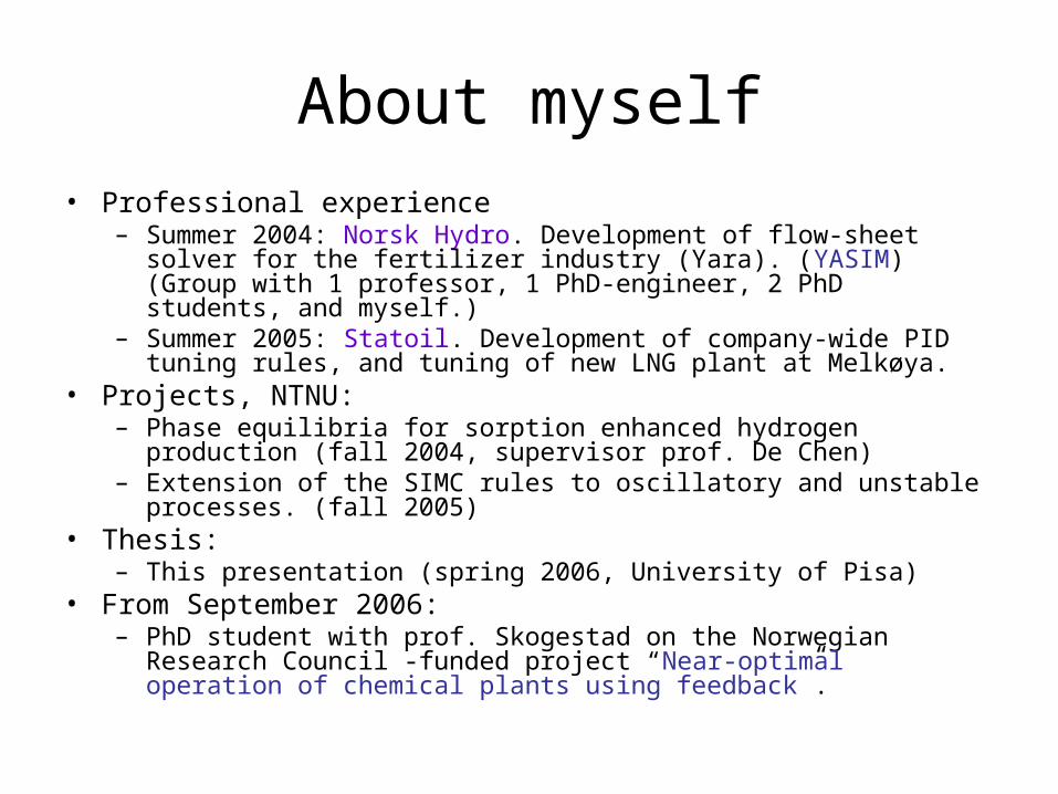
About myself• Professional experience

– Summer 2004: Norsk Hydro. Development of flow-sheet solver for the fertilizer industry (Yara). (YASIM) (Group with 1 professor, 1 PhD-engineer, 2 PhD students, and myself.)

– Summer 2005: Statoil. Development of company-wide PID tuning rules, and tuning of new LNG plant at Melkøya.

• Projects, NTNU:– Phase equilibria for sorption enhanced hydrogen production (fall 2004,

supervisor prof. De Chen)– Extension of the SIMC rules to oscillatory and unstable processes. (fall

2005)• Thesis:

– This presentation (spring 2006, University of Pisa)• From September 2006:

– PhD student with prof. Skogestad on the Norwegian Research Council -funded project “Near-optimal operation of chemical plants using feedback”.

Agenda


• Introduction to stiction and detection




• Conclusions

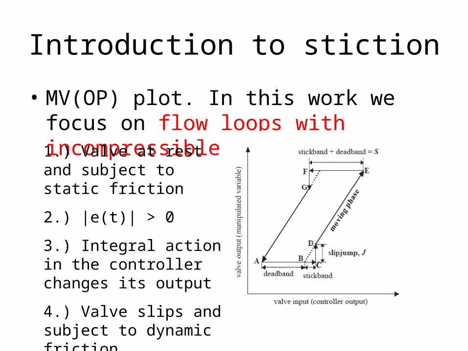
Introduction to stiction

• MV(OP) plot. In this work we focus on flow loops with incompressible fluids1.) Valve at rest and subject to static friction

2.) |e(t)| > 0

3.) Integral action in the controller changes its output

4.) Valve slips and subject to dynamic friction.

How to detect stiction

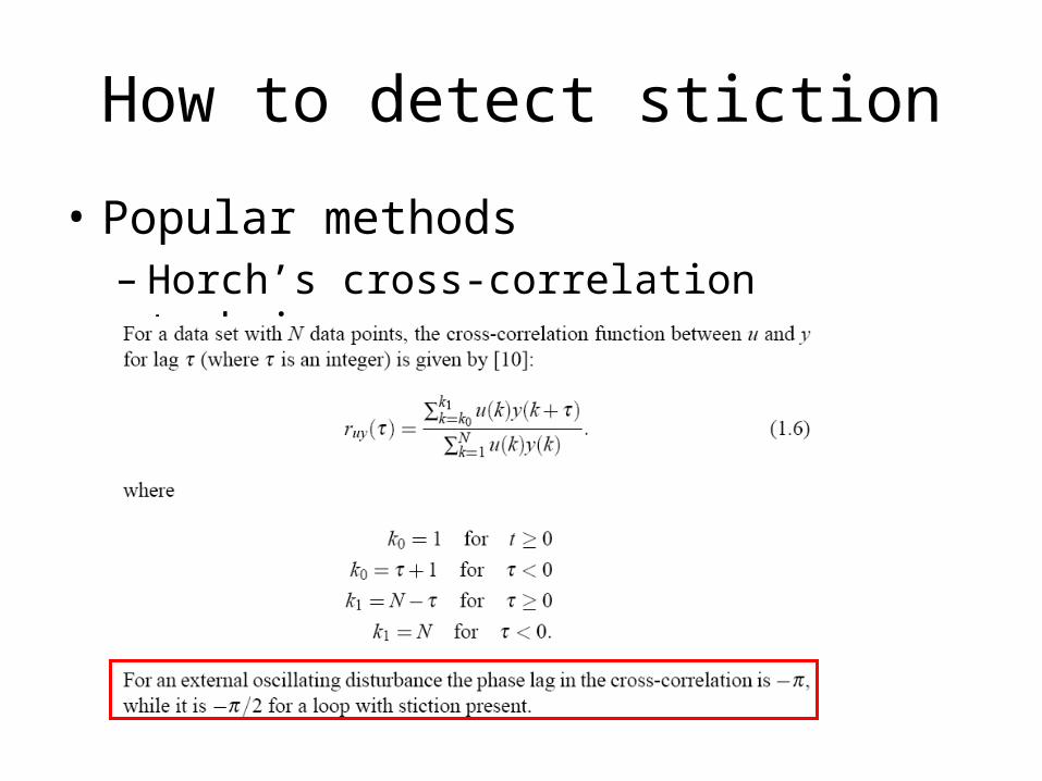
• Popular methods– Horch’s cross-correlation technique


• Popular methods– Higher-Order Statistics


• Popular methods– Curve-fitting / Relay Technique

Stiction

Agenda


• Introduction to stiction and its detection




• Conclusions


• Pattern recognition techniques

• Possible to detect the typical movements using symbolic represenations?


• Pattern recognition techniques– Neural networks

Neural network


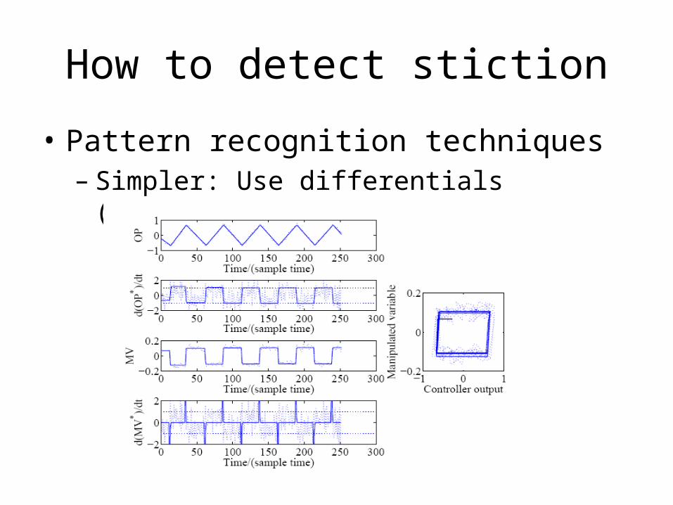
• Pattern recognition techniques– Simpler: Use differentials (Yamashita method)

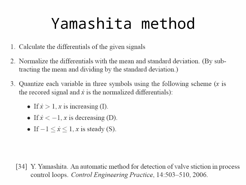
Yamashita method

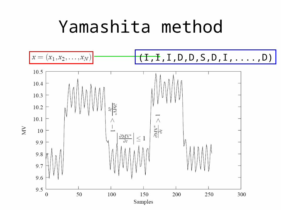
Yamashita method

(I,I,I,D,D,S,D,I,....,D)

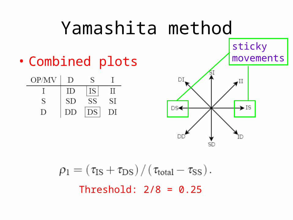
Yamashita method

• Combined plots

Threshold: 2/8 = 0.25

stickymovements

Yamashita method

• Matched index

Threshold: 2/8 = 0.25

Yamashita method

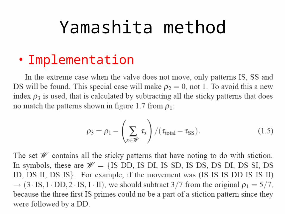
• Implementation

Yamashita method

• Application to simulated data– Choudhury model used

Yamashita method

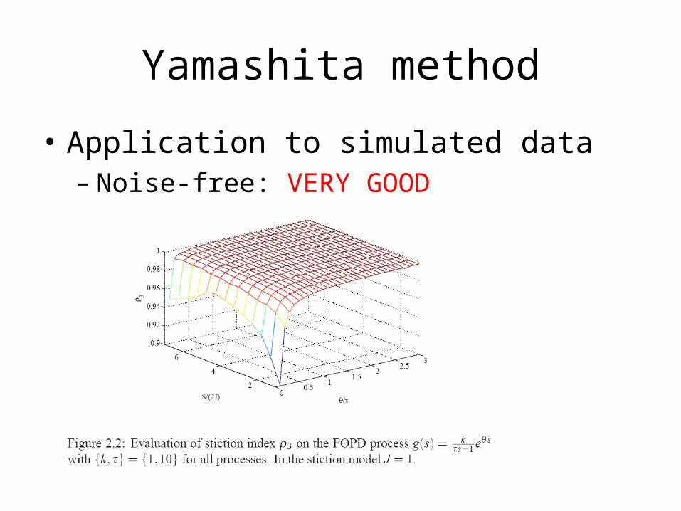
• Application to simulated data– Noise-free: VERY GOOD

Yamashita method

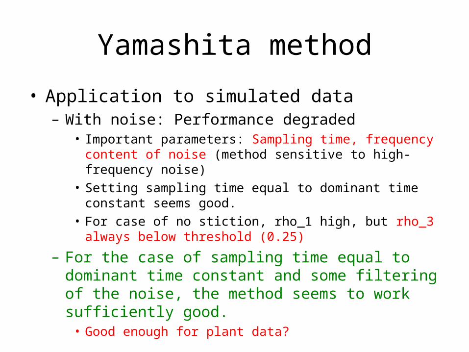
• Application to simulated data– With noise: Performance degraded

• Important parameters: Sampling time, frequency content of noise (method sensitive to high-frequency noise)

• Setting sampling time equal to dominant time constant seems good.

• For case of no stiction, rho_1 high, but rho_3 always below threshold (0.25)

– For the case of sampling time equal to dominant time constant and some filtering of the noise, the method seems to work sufficiently good.

• Good enough for plant data?

Yamashita method

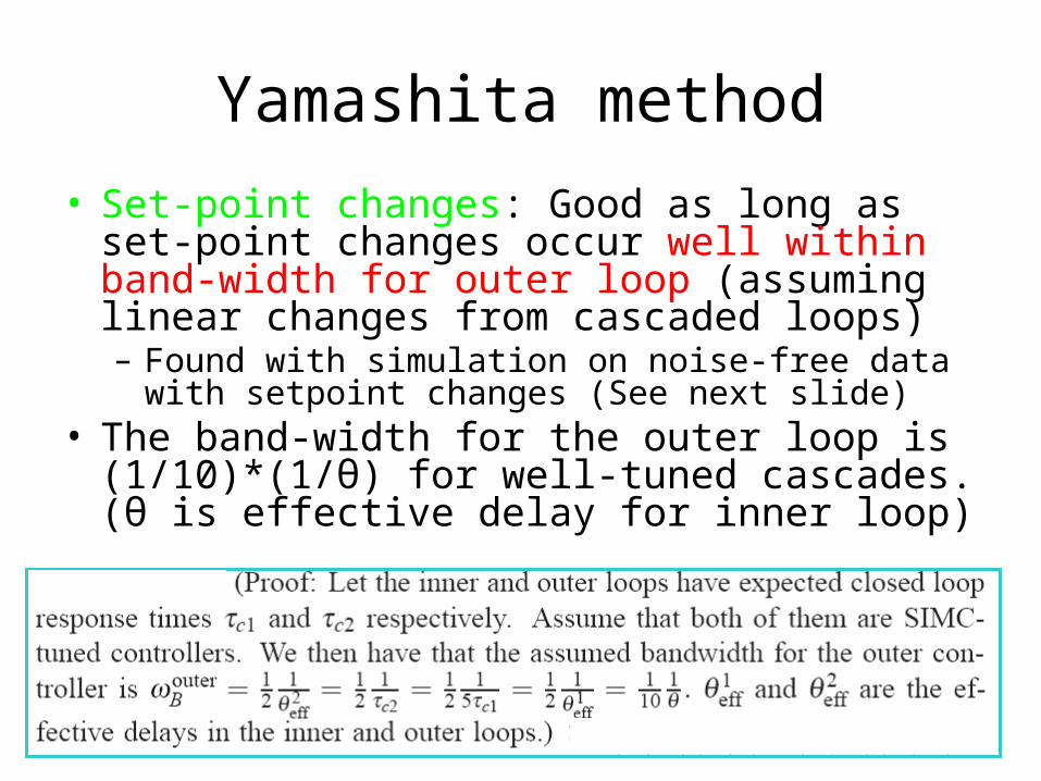
• Set-point changes: Good as long as set-point changes occur well within band-width for outer loop (assuming linear changes from cascaded loops)– Found with simulation on noise-free data with setpoint

changes (See next slide)• The band-width for the outer loop is (1/10)*(1/θ)

for well-tuned cascades. (θ is effective delay for inner loop)

Yamashita method

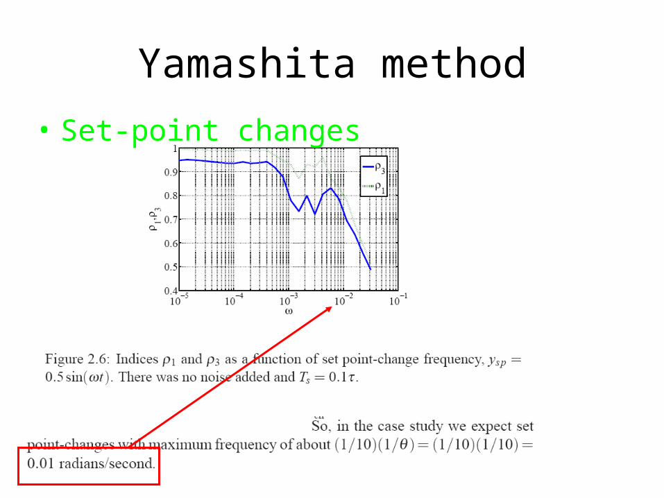
• Set-point changes

Yamashita method

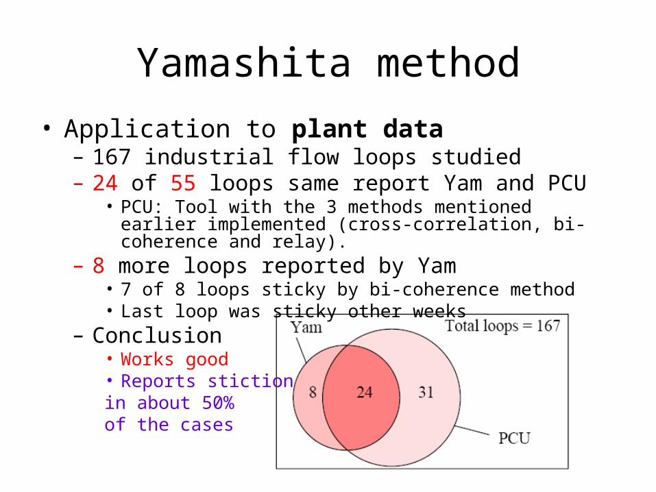
• Application to plant data– 167 industrial flow loops studied– 24 of 55 loops same report Yam and PCU

• PCU: Tool with the 3 methods mentioned earlier implemented (cross-correlation, bi-coherence and relay).

– 8 more loops reported by Yam• 7 of 8 loops sticky by bi-coherence method• Last loop was sticky other weeks

– Conclusion• Works good• Reports stictionin about 50%of the cases

Yamashita method

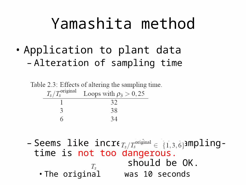
• Application to plant data– Alteration of sampling time

– Seems like increasing the sampling-time is not too dangerous. should be OK.

• The original was 10 seconds

Yamashita method

• Application to plant data– Observation window

OK toreduceobs. windowto for example720 samples

Yamashita method

• Application to plant data– Conclusions

• Detects stiction in about 50% of the cases for which the advanced package reports stiction

• Identifies the loops with clear stiction patterns

• Noise level less than worst case in simulations

720 samples

Agenda


• Introduction to stiction




• Conclusions

Patterns and explanations

• Some other patterns were found. For example:

• Possible to find physical explanation?


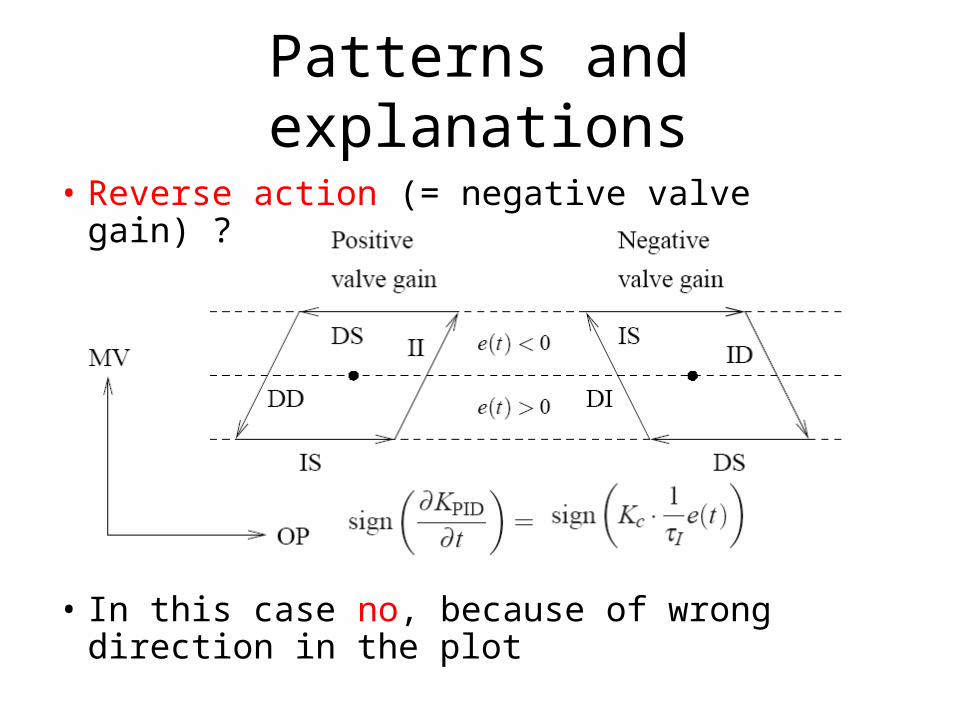
• Reverse action (= negative valve gain) ?

• In this case no, because of wrong direction in the plot


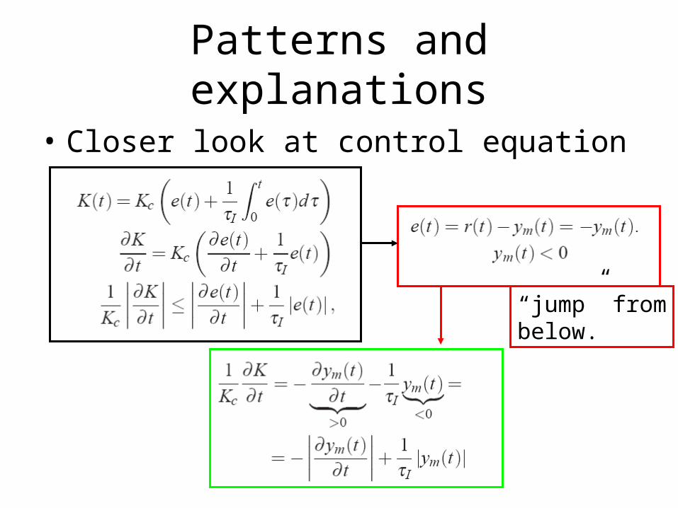
• Closer look at control equation (PI)

“jump” frombelow.


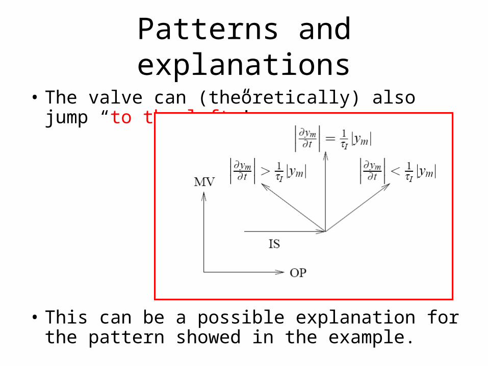
• The valve can (theoretically) also jump “to the left”!

• This can be a possible explanation for the pattern showed in the example.


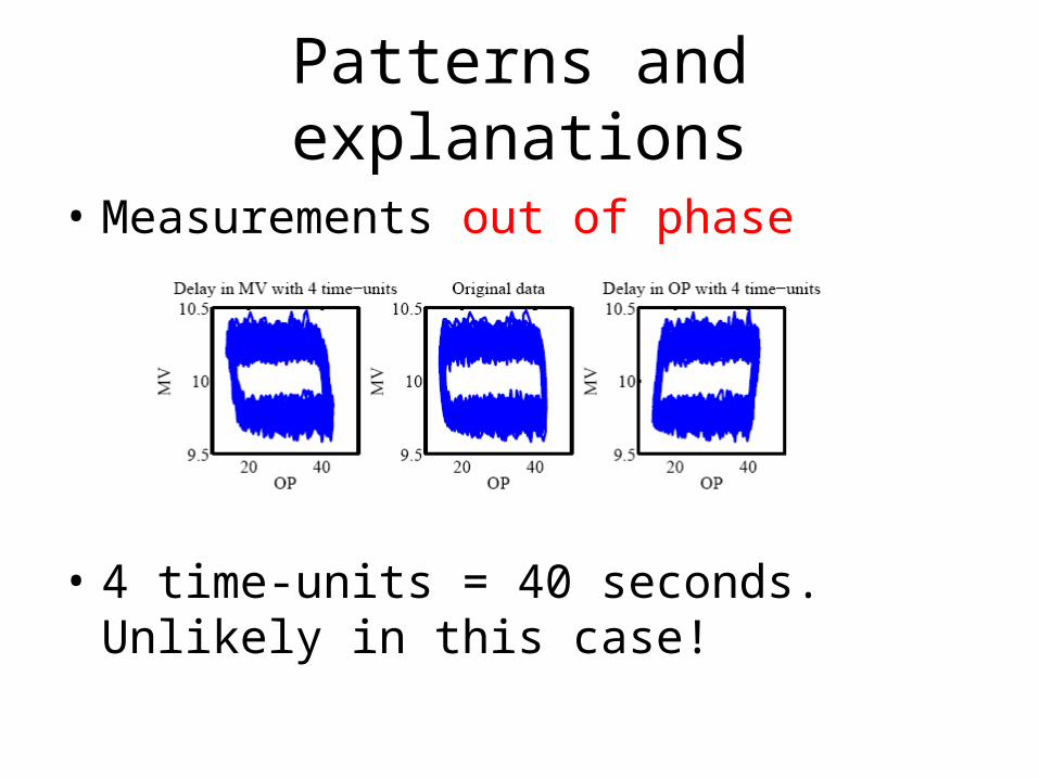
• Measurements out of phase

• 4 time-units = 40 seconds. Unlikely in this case!

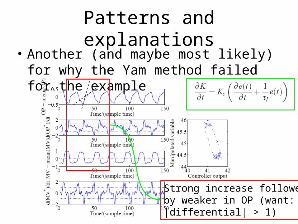
Patterns and explanations• Another (and maybe most likely) for why

the Yam method failed for the example

Strong increase followedby weaker in OP (want: |differential| > 1)


• Conclusions– More insight into control action on sticky

valves achieved. The Yamashita method can easily be extended to cover to cover other known patterns. The “theoretical considerations” in this chapter needs to be checked with real valves.

Agenda






• Conclusions

Quantification

Some work already done at the lab with a method developed and implemented in the PCU.– As with stiction detection methods, it could be

nice with more methods.– Necessary, as thedetection methodsdon’t report amount of stiction

Quantification

• Basis: Bi-coherence method. FFT-filteringby setting allunwanted coefficients to zero and then take the inversetransform to getfiltered data

Quantification

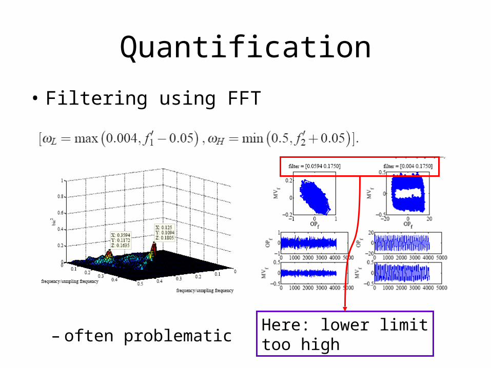
• Filtering using FFT

– often problematicHere: lower limittoo high

Quantification

• Filtering using FFT– Conclusion

• Need steady data (best with little SP-changes)• Few examples of suitable data in our plant data• Using default filter limits did not work good• Still needs tuning

– Before industrial implementation quite a lot of work needs to be conducted

Quantification

• Chose to move on to ellipsis fitting...– 3 different methods

• Simple centered and unrotated ellipse

• General conic with two different constraint specifications (more details in the next slides)

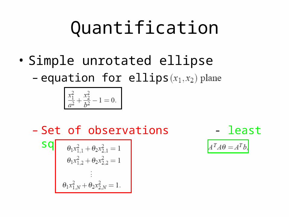
Quantification

• Simple unrotated ellipse– equation for ellipse in the

– Set of observations - least squares

Quantification

• General conic

• Easier: set c = -1 and solve by least squares directly

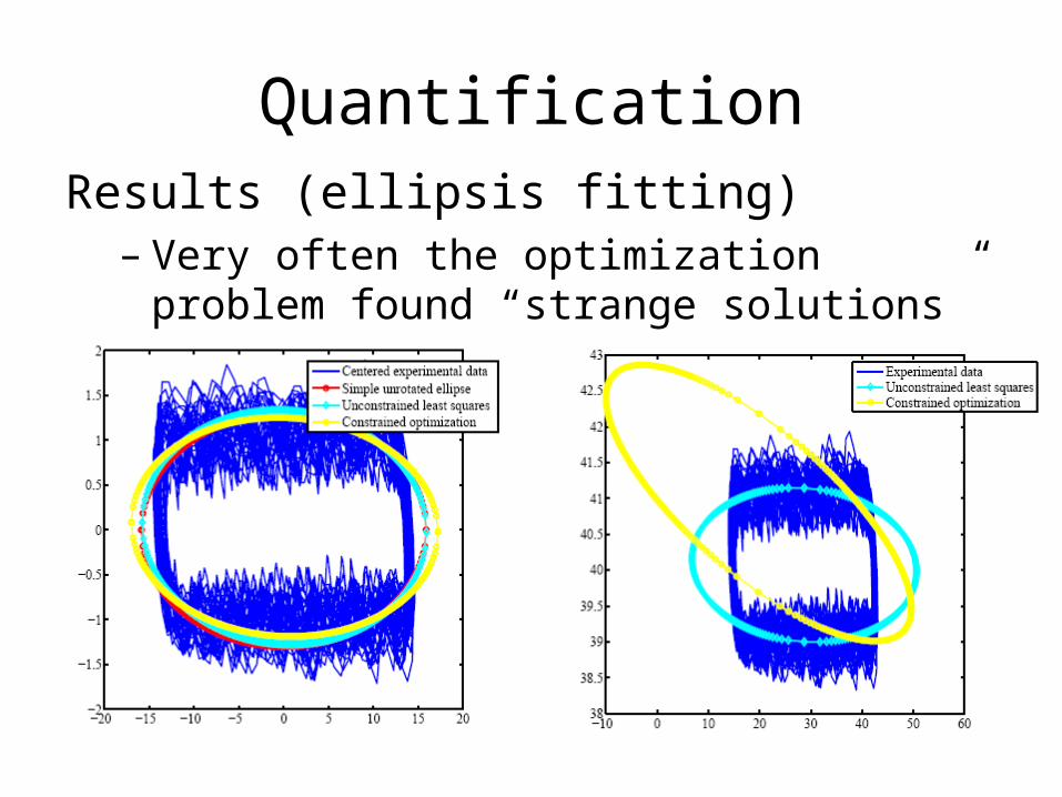
QuantificationResults (ellipsis fitting)

– Very often the optimization problem found “strange solutions” (often imaginary axes)

Quantification

• Discussion (ellipsis)– Does guarantee an ellipsis? (Probably

not) (See report for derivation)– Setting seems more promising– Obviously still work to do here!

• Answer questions given above• Consider other techniques, such as clustering

techniques

Quantification

• Conclusions– The work did not give “industrial-ready” results– I got more insight into time-domain -> frequency

domain filtering (“FFT”-filtering)

Agenda






• Conclusions

Conclusions

• Yamashita method proved to work good on industrial data. Findings submitted to ANIPLA 2006 as a conference paper.

• Hopefully the thesis gives more insight into patterns in sticky valves in MV(OP) plots.

• Introductory work to filtering and ellipsis fitting for quantification conducted.

References

• See thesis for complete bibliography

• Thesis should be available from Sigurd Skogestads homepage, www.nt.ntnu.no/users/skoge– Diploma students -> 2006 ->

manum– Contains more details about

everything and also description about software developed.

http://www.nt.ntnu.no/users/skoge

analysis of techniques for automatic detection and quantification of stiction in control loops...

Documents