Wireless Networks 8, 107–120, 2002 2002 Kluwer Academic Publishers. Manufactured in The Netherlands.

Analysis of a Metropolitan-Area Wireless Network

DIANE TANGStanford University, Gates 3A, Stanford, CA 94305-9030, USA

MARY BAKERStanford University, Gates 4A, Stanford, CA 94305-9040, USA

Abstract. We analyze a seven-week trace of the Metricom metropolitan-area packet radio wireless network to find how users take advantageof a mobile environment. Such understanding is critical for planning future large-scale mobile network infrastructures. Amongst otherresults, we find that users typically use the radios during the day and evening. Of the users who move around during the trace (over half),we find that the more locations a user visits on a daily basis, the closer together, on average, those locations are. While these results areonly known to be valid for this particular network, we hope future analysis of other networks will add to a growing understanding of mobilenetwork behavior.

Keywords: metropolitan-area wireless network, network analysis

1. Introduction

Currently, mobile and ad hoc networking is the topic of manyresearch and development efforts. Much of this work focuseson providing future users with network resources and con-nectivity no matter where they are. Whether the work con-centrates on adapting applications to changing user locationor on devising new protocols to handle mobility, it is largelybased on assumptions of how users will take advantage of amobile environment. It is difficult to verify these assump-tions since we are unaware of any publicly available studiesof a sizeable metropolitan-area wireless network. Therefore,many research and development efforts must drive their sim-ulations using assumed models of user movement not derivedfrom observation.

In this paper, we analyze a network trace of the Metricompacket radio network, a metropolitan-area wireless network,to find answers to overall network questions such as when themobile network is the most active, how active the networkgets, where the network is active, as well as radio mobilityquestions such as how far, how often, and when users move.The answers to such questions are crucial in planning a futuremobile network infrastructure, and in understanding how peo-ple actually take advantage of a mobile network. While theseresults are only known to be valid for this particular network,we hope future analysis of other networks will add to a grow-ing understanding of mobile network behavior.

We present several results in this paper, including our find-ing that the more locations users visit on a daily basis, thecloser together, on average, those locations are. In addition,the distance users move is a Gaussian distribution around theradius of the network. We also find that radios are used mostlyduring the day and evening hours.

In this paper, we first present some background informa-tion about the data before we present the actual results from

the analysis. The analysis is divided into two parts: overallnetwork behavior and radio mobility.

2. Background

In this section, we describe the network traced, how the datawas collected, and some issues that arose in the data analysis.

2.1. Data collection

The traces we study here were obtained from Metricom [2,6].Metricom has installed a RicochetTM packet radio networkinfrastructure in three major metropolitan areas (San Fran-cisco Bay Area, Washington D.C., and Seattle), as well as insome airports, hotels, and college campuses scattered acrossthe United States. This infrastructure consists of “poletop”repeaters distributed throughout the covered areas. Each po-letop is one of two types:

• a wireless repeater, which just forwards packets on to an-other poletop via the radio interface, or

• a wired access point, which has both a radio interface anda wired interface. Typically, wired access points have 8,16, or 24 radios on them, as they are the focal point ofmany other wireless repeaters.

The range of a repeater is normally about half a mile. Thisrange may vary depending on external conditions, such as theweather or the location of buildings and hills.

When a subscriber radio is first turned on, it scans the net-work for poletops, and chooses one with which to register.This choice is usually based on signal strength, but may alsobe based on load-balancing considerations. This poletop is re-sponsible for forwarding all packets to and from the Metricomnetwork on behalf of that radio. Radio registrations also occur

108 TANG AND BAKER

whenever the radio changes its primary poletop and accord-ing to a predetermined pattern when the radio is stationary(see section 5.2). Note that while a radio registers with onlyone poletop at a time, the radio does keep an internal list ofall poletops within its range. Each registration, whether at thesame or at a different primary poletop, is logged by a centralnameserver.

The trace consists of a nameserver log covering a seven-week period from February 1, 1998, through March 23, 1998,with the exception of three holes in the trace data, duringwhich no registrations were logged: February 16, 6 a.m.through 1 p.m.; February 16, 5 p.m., through February 17,4 a.m.; and February 17, 4 p.m., through February 18, noon.The network at the time of the trace consisted of 14,053 pole-tops and 24,773 radios.

There were a total of 7,726,678 events logged over theseseven weeks. Of those, 5,982,846 are registrations and theother 1,743,832 are queries. A registration occurs when theradio informs the nameserver of its current primary pole-top, i.e., the poletop to which packets destined for this radioshould be sent. A query occurs when the radio queries thenameserver about some other entity in the network, such asanother radio or poletop. Queries are usually made at the startof a connection, and the radio can register at different pole-tops while a connection is on-going.

Each log entry consists of the following information:

• a timestamp taken at the nameserver with accuracy to thesecond,

• a sequence number,

• the radio id,

• the wired access point used,

• the name of the radio’s choice for primary poletop,

• whether the entry is a registration or a query.

A poletop’s name is an encoding of its latitude and lon-gitude, so given a poletop’s name, we can determine its ge-ographic location and therefore the approximate geographiclocation of the radio registering with it.

2.2. Data analysis techniques

In analyzing this trace, the main difficulty is in dealing withthe sheer volume of data – 7,726,678 events, 24,773 radios,and 14,053 poletops – making it impractical, if not impossi-ble, to look at each radio by hand. As a result, we neededmethods to help gather our results automatically. We turnedto a technique commonly used in data mining and machinelearning called clustering, also known as an unsupervisedlearning technique.

Clustering algorithms take a set of points in n-dimensionalspace and find coherent subsets. Each subset consists ofpoints that are clustered together. The advantages of usingclustering algorithms are the ability to categorize radios au-tomatically, and the ability to find groupings that we mightnot otherwise find. The disadvantages are that the results aredependent on the parameters and distance functions used.

We use three different clustering algorithms:

• k-means [9], an iterative clustering algorithm,

• hierarchical agglomerative clustering [8], a tree-formingclustering algorithm, and

• expectation-maximization (EM) [3], a method to find themeans and variances of a mixture of Gaussian distribu-tions. EM is especially useful when the range of valuesdiffers widely between dimensions.

We use both hierarchical agglomerative and k-means clus-tering algorithms to help determine when a radio has movedby grouping poletops into clusters, which we also refer to aslocations. Without physically moving, the radio may still bewithin range of up to 20 different poletops at the same timeand may, therefore, register at any of these poletops. We de-termine that a radio has moved when it registers with a pole-top in a different cluster (a different location). In section 4,we use both EM and k-means to categorize the radios intodifferent patterns of mobility.

3. Overall network behavior

The first three questions we asked have to do with overallnetwork usage:

1. When is the network the most active?

2. How active does the network get?

3. Where is the network the most active?

The answers to these questions can help network plannersplan future extensions to the network infrastructure. Also,they provide a way both to compare a simulated network to anactual network and to provide a basis for simulated networks.

To summarize the results presented in this section, we findthat the network is more active on weekdays than on week-ends, that the most active poletops handle up to 182 distinctradios an hour and handle over 1,600 registrations an hour,and that the network is most active where there is a high con-centration of technical people. We now look at each questionin more detail.

To answer the first question, figure 1 shows that the net-work is more active on weekdays, especially the days in themiddle of the week. This pattern holds regardless of whetherwe are looking at all events, registrations only, or queries only.Figure 2 shows that the network is least active between 3 a.m.and 5 a.m., when most people are asleep. The two lines infigure 2, one lower in the evening hours and one higher, cor-respond to weekend and weekdays respectively. Even in Sil-icon Valley, where the majority of radio users and poletopsare, people are less likely to work on weekends. There is aslight decrease in the number of active radios during weekdayevenings, perhaps corresponding to when people stop work-ing for the day. There is also a slight rise around 8 p.m. onweekends. We define an active radio as one that has at leastone registration or query logged at the nameserver within thegiven time period.

ANALYSIS OF A METROPOLITAN-AREA WIRELESS NETWORK 109

Figure 1. Histogram of the number of active radios on each day of the trace.One corresponds to Sunday, two to Monday, etc. There is a dip around the

16th through the 18th days corresponding to the holes in the trace data.

Figure 2. Graph showing the average, minimum, and maximum number ofactive radios for each hour of the trace. The two sets of lines, one lower inthe evening hours and one higher, correspond to the weekend and weekdaysrespectively. We ignore those days containing the holes in the trace during

which no events were logged.

To find out how active the network gets, for each poletopwe first count how many distinct radios register with or queryfrom that poletop over the course of the trace. This rangesfrom handling only one distinct radio event over the course ofthe entire trace to handling 6,677 events (6,064 registrations,434 queries), which occurs at the poletop at Metricom head-quarters. Figure 3 shows the distribution within this range.

Figure 3. Cumulative histogram of the number of poletops (y-axis) that han-dle a certain number of distinct active radios over the course of the entiretrace (x-axis). Note that to show the detail, we cut off the tail of the graph,which extends out to 6,677 radios for all events, 6,064 radios for registrations

only, and 434 radios for queries only.

Figure 4. Two-variable histogram, where the darkness of the bar reflects thenumber of poletops that receive events from a given number of radios, byhour of the day. No matter what time of day it is, most poletops see eventsfrom fewer than 10 radios in an hour. The largest number of radios a poletopreceives events from within an hour is 182. Note that the maximum numberof radios at any point in the graph is the total number of poletops (14,053)multiplied by the number of times that hour occurs during the trace (once for

each of the 52 days).

We also examine how many radios and radio events perhour a poletop needs to handle. Figure 4 shows that whilethe majority of poletops only handle one radio an hour, some

110 TANG AND BAKER

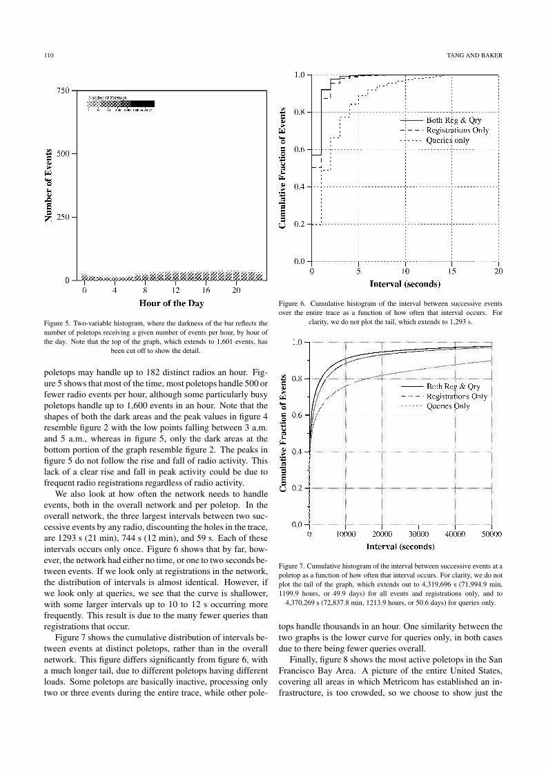
Figure 5. Two-variable histogram, where the darkness of the bar reflects thenumber of poletops receiving a given number of events per hour, by hour ofthe day. Note that the top of the graph, which extends to 1,601 events, has

been cut off to show the detail.

poletops may handle up to 182 distinct radios an hour. Fig-ure 5 shows that most of the time, most poletops handle 500 orfewer radio events per hour, although some particularly busypoletops handle up to 1,600 events in an hour. Note that theshapes of both the dark areas and the peak values in figure 4resemble figure 2 with the low points falling between 3 a.m.and 5 a.m., whereas in figure 5, only the dark areas at thebottom portion of the graph resemble figure 2. The peaks infigure 5 do not follow the rise and fall of radio activity. Thislack of a clear rise and fall in peak activity could be due tofrequent radio registrations regardless of radio activity.

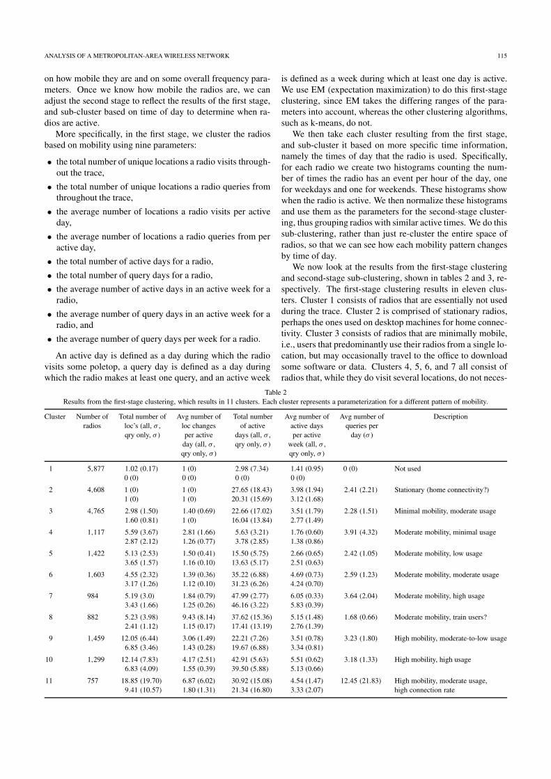
We also look at how often the network needs to handleevents, both in the overall network and per poletop. In theoverall network, the three largest intervals between two suc-cessive events by any radio, discounting the holes in the trace,are 1293 s (21 min), 744 s (12 min), and 59 s. Each of theseintervals occurs only once. Figure 6 shows that by far, how-ever, the network had either no time, or one to two seconds be-tween events. If we look only at registrations in the network,the distribution of intervals is almost identical. However, ifwe look only at queries, we see that the curve is shallower,with some larger intervals up to 10 to 12 s occurring morefrequently. This result is due to the many fewer queries thanregistrations that occur.

Figure 7 shows the cumulative distribution of intervals be-tween events at distinct poletops, rather than in the overallnetwork. This figure differs significantly from figure 6, witha much longer tail, due to different poletops having differentloads. Some poletops are basically inactive, processing onlytwo or three events during the entire trace, while other pole-

Figure 6. Cumulative histogram of the interval between successive eventsover the entire trace as a function of how often that interval occurs. For

clarity, we do not plot the tail, which extends to 1,293 s.

Figure 7. Cumulative histogram of the interval between successive events at apoletop as a function of how often that interval occurs. For clarity, we do notplot the tail of the graph, which extends out to 4,319,696 s (71,994.9 min,1199.9 hours, or 49.9 days) for all events and registrations only, and to

4,370,269 s (72,837.8 min, 1213.9 hours, or 50.6 days) for queries only.

tops handle thousands in an hour. One similarity between thetwo graphs is the lower curve for queries only, in both casesdue to there being fewer queries overall.

Finally, figure 8 shows the most active poletops in the SanFrancisco Bay Area. A picture of the entire United States,covering all areas in which Metricom has established an in-frastructure, is too crowded, so we choose to show just the

ANALYSIS OF A METROPOLITAN-AREA WIRELESS NETWORK 111

Figure 8. Picture of the San Francisco Bay Area. Each dot corresponds to apoletop. The darker the dot, the more radios visit that poletop over the course

of the trace.

Figure 9. Histogram of the distance between successive events in the networkby any radio as a function of how often that distance occurs.

Bay Area since it has the highest concentration of poletops.The darker dots correspond to the more active poletops. Sev-eral hot spots are worth noting. First, the dark area in SanFrancisco corresponds to the Financial District. The secondstrip of scattered dark dots running northwest-southeast corre-sponds to Highway 101, on which many high tech companieshave their headquarters. Another hot spot is the dark dot in theupper part, which corresponds to Berkeley. Also, towards thebottom is a hot spot corresponding to Metricom headquarters.The lowest island of activity corresponds to Santa Cruz.

We also want to investigate how the activity in the networkis distributed geographically, rather than temporally as shownin figure 6. Now we look at the interval in distance betweensuccessive events in the entire network. As we can see in fig-ure 9, there are several common distances: 100 miles or less,around 650 miles, around 1000 miles, 1400 miles, 2000 miles,and 2400 miles. These distances all correspond either to traf-fic within a Metricom installation or to the approximate dis-tances between various Metricom installations. Because theBay Area contains about 65% of the poletops in the Metricominfrastructure, distances of 100 miles or less are prevalent. Inother words, two successive registrations in the network aremore likely to both be in the Bay Area than to be distributedacross the country. However, we can see a Gaussian distribu-tion around each of the common distances. This implies thatgiven the radius of the network, the distance between regis-trations of any radio in the network is likely to be a Gaussiandistribution around the radius.

4. Radio mobility

The other major set of questions we want to answer concernsradio mobility:

1. How often do radios move?

2. How far do they move?

3. Can we identify patterns of mobility?

Answering these questions is crucial for understandingwhether and how people actually take advantage of a mo-bile environment. Also, understanding current radio mobil-ity helps in choosing parameters for simulations of mobilenetworks. Unrealistic movement models lead to unrealisticsimulation results.

To summarize the results in this section, we first find thatusers who are mobile do not move frequently, and that 64%of all users only appear at one location per day. As for howfar users move, most users move within their local area, withfewer users traveling the long distances between differentMetricom installations. In addition, as the number of loca-tions visited by a user increases, the average distance traveledbetween each location decreases. Finally, we are able to findpatterns of mobility for users, such as the number of userswho are active both day and night versus users active onlyduring the day. We now examine these findings in more de-tail.

We first calculate the number of different poletops and lo-cations at which radios register over the course of the trace.Figure 10 shows that 42% of all radios are stationary, and that64% of all radios visit only one location a day. This impliesthat although users do move around with their laptops, themovement is not very frequent. We can also see the differencebetween looking at poletops versus locations. While 42% ofradios are stationary with respect to location, only 16% ofradios are stationary with respect to poletops, meaning thatradios often register with poletops that fall in the same clus-ter or general area. Our location finder underestimates user

112 TANG AND BAKER

Figure 10. Cumulative histogram of the percentage of radios that visit a givennumber of poletops, locations, or locations per day, over the course of thetrace. For example, 64% of radios visit only one location per day, 42% visitonly one location over the course of the entire trace, and 16% of radios visitonly one poletop over the course of the entire trace. Note that to show thedetail, we cut off the tail of the graph, which extends to 25 locations per day,

176 locations, and 1,025 poletops.

Figure 11. Histogram of the average, minimum, and maximum number of ra-dios changing locations during a particular hour of the day. The time plotted

is the second of two successive events.

mobility, so there may be more actual locations than we havefound (see section 5.3).

We also measure how many radios appear, i.e., register orquery, at a different location from their last appearance. Fig-ure 11 shows these results. Unsurprisingly, this rate mimicsthe usage graph in figure 2, with anywhere from 122 (0.5%)

Figure 12. Cumulative histogram of the number of events as a functionof the distance traveled. Note that the tail of the graph (which extends to2,576 miles) has been removed to show detail. Also note that each pair ofcorresponding poletop and location lines converge at one mile. The straightline between 0 and 1 miles for the location graphs reflects the fact that loca-tions cluster poletops together: poletops that are close together are consideredto be a single location, and therefore, represent a movement of distance zero.

to 1,484 (6.0%) radios changing location at a time. There are,however, some interesting features to the weekday curve infigure 11. First, there is a dip around 11 a.m. to 2 p.m., ap-proximately corresponding to lunchtime, showing that manypeople do not take their laptops to lunch wih them. Second,there is an increase in the number of radios changing locationaround 5 p.m., about when many people stop working for theday. We still observe the dip in the weekday evenings similarto figure 2.

We next look at how far a radio moves when it changes itsprimary poletop or location. Figure 12 shows the distributionof how often radios move a given distance, in terms of move-ment both between poletops and between locations. Over79% of the events (or 80% of registrations, 90% of queries)involve no change in location. If we then look at figure 13,we can see that while the majority of successive events occurwithin 50 miles of one another, there are small peaks cor-responding to the long-distance routes between airports andmajor cities in which Metricom has established an infrastruc-ture. While this graph looks similar to figure 9, cross-countryregistrations are much less frequent when examining individ-ual user behavior rather than overall network behavior.

We further examine radio movement in table 1, whichshows the breakdown of radios by how often they move, bothoverall and per day, and how far they move. First, a radio thatvisits more locations overall does not necessarily also appearat proportionally more locations per day. For instance, themajority of radios that visit three or more locations overallstill only appear at one to two locations on a daily basis. Fur-thermore, only 3.5% of radios that visit more than four loca-

ANALYSIS OF A METROPOLITAN-AREA WIRELESS NETWORK 113

tions overall appear at more than four locations per day on av-erage. (Note that one distinct location may be counted as mul-tiple visited locations per day. For example, a user that visitslocation A followed by location B before returning to loca-tion A in one day is counted as appearing at three locations inthat day.) This result implies that users who visit many loca-tions do not necessarily move around more on a daily basis,

Figure 13. Histogram of the percentage of successive events from a radio as afunction of the distance traveled between those events. Note the logarithmic

scale on the y-axis.

but rather visit the different locations over a longer period ofseveral days or weeks.

More surprisingly, as the number of locations visited on adaily basis increases, the average distance traveled decreases.In other words, the more someone moves around each day,the closer the locations are. This overall decreasing trend maycorrespond to the flatter distribution of the range of distancesamong users who visit multiple locations per day, althoughthe majority of locations are still relatively close together.This distribution could stem, for example, from users usingtheir laptops on a train, such as the train that runs along High-way 101, causing them to “visit” numerous locations on theirway to work.

Users who visit one location per day, independent of thetotal number of locations visited throughout the trace, have alarge discrepancy between the average distance traveled andthe median distance traveled. This discrepancy is likely theresult of these users actually being split into two sub-groups:those who travel locally (for example, people who take theirlaptops home on the weekends), and those who travel longdistances (perhaps people who only use their laptops whentravelling). The median distance traveled reflects the usagepatterns of this first sub-group, while this second sub-group ofusers increases the average distance traveled for all the groupsof users who, independent of the total number of locationsvisited throughout the trace, only visit one location per day.

Despite this overall decreasing trend in the average dis-tance, the median distance stays relatively constant, reflectingthe many users who only move short distances. Further, the

Table 1How far users move depending on how many locations and locations per day a user visits. For example, 510 users visit only two locations throughout the

entire trace, but on average, visit between one and two locations per day.

Number of Number of Average Median Number of locations Number of Average Medianlocations radios (%) distance distance per active day (max) radios (%) distance distance

1 10,459 (42.2%) 0 0 1 (1.0) 10,459 (100%) 0 0

2 2,746 (15.1%) 6.9 2.9 1 (1.0) 2,152 (84.1%) 11.6 1.61–2 (1.98) 510 (13.6%) 2.1 1.7

2 (2.0) 84 (2.3%) 1.7 1.3

3 2,371 (9.6%) 5.2 1.6 1 (1.0) 1,367 (57.7%) 11.3 1.71–2 (1.98) 914 (38.5%) 3.5 1.6

2 (2.0) 47 (2.0%) 2.3 1.92–3 (2.92) 31 (1.3%) 2.3 2.0

3 (3.0) 12 (0.5%) 2.2 2.2

4 1,694 (6.8%) 4.2 1.5 1 (1.0) 569 (33.6%) 8.4 1.61–2 (1.98) 1,013 (59.8%) 4.6 1.5

2 (2.0) 44 (2.6%) 2.3 1.52–3 (2.98) 55 (3.2%) 2.1 1.5

3 (3.0) 3 (0.2%) 2.0 1.93–4 (3.65) 8 (0.5%) 1.5 1.3

4 (4.0) 2 (0.1%) 7.9 2.7

>4 6,503 (26.3%) 7.9 2.4 1 (1.0) 438 (6.7%) 12.2 1.71–2 (1.98) 4,434 (68.2%) 11.2 1.8

2 (2.0) 126 (1.9%) 4.2 1.32–3 (2.98) 1,020 (15.8%) 4.9 1.7

3 (3.0) 36 (0.5%) 6.0 1.73–4 (3.96) 210 (3.2%) 4.3 2.0

4 (4.0) 13 (0.2%) 4.3 2.0>4 (24.48) 226 (3.5%) 8.0 6.9

114 TANG AND BAKER

Figure 14. Cumulative histogram of the number of times a certain number ofregistrations occur before a query. Note that to show the detail, we cut off the

tail of the graph which extends to 7,948 registrations between queries.

average and median distances, in terms of the total numberof locations visited rather than the average number of loca-tions visited per day, are also relatively constant, implyingthat movement is dependent more on how many locations auser visits on a daily basis than on how many locations a uservisits overall.

4.1. Radio queries

Before we look into categorizing radios into different pat-terns of mobility, we examine radio behavior with respect toqueries. Queries are usually made when a radio makes a newconnection, although some radios are used as part of Metri-com’s diagnostic utilities and make many more queries thanare normal. Note that a query is made regardless of whetherthe user is using the radio in modem mode or StarMode (orpacket mode) [2]. If the radio is being used in StarMode, theradio could have multiple outstanding connections at a time.Since we do not have information about the end of a connec-tion, we do not account for this situation. Using the radios inmodem mode is prevalent, however. Because very few radiosare used for diagnostic purposes and very few radios are usedin StarMode, we believe that our results are a good approxi-mation.

Our main interest with regard to queries is in how muchactivity there is between queries. We first look at how manytimes radios register between queries. Figure 14 shows the cu-mulative distribution of how many registrations occur beforea query, which is indicative of the amount of activity betweenthe beginnings of different connections. The majority of con-nections occur after 30 or fewer registrations. In figure 15,we examine how often a radio changes its location or poletopbefore starting a connection. This graph is indicative of how

Figure 15. Cumulative histogram of how often a certain number of poletopsor locations are registered at before a query is made. Note that to show thedetail, we cut off the tail of the graph which extends to 1,193 locations and

3,334 poletops.

much movement there is between connections. Note that aconnection can be long-lived and last for days, explaining thetail of the graph, which extends out to 1,193 locations or 3,334poletops. Also note that we count the number of changes inlocation; if a radio visits location A then B then C then B andthen A again, we count this sequence as four location changes.We see in figure 15 that 70.4% of connections have no move-ment before them at all, while 95% of radios change locationfewer than four times. In other words, most radios do notmove around much between connections. Unfortunately, wedo not have information about when connections terminate sowe do not know how much of the movement occurs while theconnection itself is maintained.

4.2. Patterns of mobility

Our final goal is to categorize the radios into different pat-terns of mobility. One expected pattern, for example, mightcorrespond to a user who moves between using the radio athome and at the office. Another pattern would correspond tothe user who just uses the radio at home. Yet another patternmight correspond to a traveling salesman who uses the radioto keep in touch with the warehouse. We are interested inthese patterns to see whether and how people take advantageof mobility.

Without comprehensively going through the radios byhand, there is no way to find all the categories, much less cat-egorize each radio, without using clustering algorithms. Weuse a two-stage clustering because it avoids the difficulty infinding a single stage clustering that balances both the lo-cation and time information together. By separating out theclustering into two stages, we can first cluster the radios based

ANALYSIS OF A METROPOLITAN-AREA WIRELESS NETWORK 115

on how mobile they are and on some overall frequency para-meters. Once we know how mobile the radios are, we canadjust the second stage to reflect the results of the first stage,and sub-cluster based on time of day to determine when ra-dios are active.

More specifically, in the first stage, we cluster the radiosbased on mobility using nine parameters:

• the total number of unique locations a radio visits through-out the trace,

• the total number of unique locations a radio queries fromthroughout the trace,

• the average number of locations a radio visits per activeday,

• the average number of locations a radio queries from peractive day,

• the total number of active days for a radio,

• the total number of query days for a radio,

• the average number of active days in an active week for aradio,

• the average number of query days in an active week for aradio, and

• the average number of query days per week for a radio.

An active day is defined as a day during which the radiovisits some poletop, a query day is defined as a day duringwhich the radio makes at least one query, and an active week

is defined as a week during which at least one day is active.We use EM (expectation maximization) to do this first-stageclustering, since EM takes the differing ranges of the para-meters into account, whereas the other clustering algorithms,such as k-means, do not.

We then take each cluster resulting from the first stage,and sub-cluster it based on more specific time information,namely the times of day that the radio is used. Specifically,for each radio we create two histograms counting the num-ber of times the radio has an event per hour of the day, onefor weekdays and one for weekends. These histograms showwhen the radio is active. We then normalize these histogramsand use them as the parameters for the second-stage cluster-ing, thus grouping radios with similar active times. We do thissub-clustering, rather than just re-cluster the entire space ofradios, so that we can see how each mobility pattern changesby time of day.

We now look at the results from the first-stage clusteringand second-stage sub-clustering, shown in tables 2 and 3, re-spectively. The first-stage clustering results in eleven clus-ters. Cluster 1 consists of radios that are essentially not usedduring the trace. Cluster 2 is comprised of stationary radios,perhaps the ones used on desktop machines for home connec-tivity. Cluster 3 consists of radios that are minimally mobile,i.e., users that predominantly use their radios from a single lo-cation, but may occasionally travel to the office to downloadsome software or data. Clusters 4, 5, 6, and 7 all consist ofradios that, while they do visit several locations, do not neces-

Table 2Results from the first-stage clustering, which results in 11 clusters. Each cluster represents a parameterization for a different pattern of mobility.

Cluster Number of Total number of Avg number of Total number Avg number of Avg number of Descriptionradios loc’s (all, σ , loc changes of active active days queries per

qry only, σ ) per active days (all, σ , per active day (σ )day (all, σ , qry only, σ ) week (all, σ ,qry only, σ ) qry only, σ )

1 5,877 1.02 (0.17) 1 (0) 2.98 (7.34) 1.41 (0.95) 0 (0) Not used0 (0) 0 (0) 0 (0) 0 (0)

2 4,608 1 (0) 1 (0) 27.65 (18.43) 3.98 (1.94) 2.41 (2.21) Stationary (home connectivity?)1 (0) 1 (0) 20.31 (15.69) 3.12 (1.68)

3 4,765 2.98 (1.50) 1.40 (0.69) 22.66 (17.02) 3.51 (1.79) 2.28 (1.51) Minimal mobility, moderate usage1.60 (0.81) 1 (0) 16.04 (13.84) 2.77 (1.49)

4 1,117 5.59 (3.67) 2.81 (1.66) 5.63 (3.21) 1.76 (0.60) 3.91 (4.32) Moderate mobility, minimal usage2.87 (2.12) 1.26 (0.77) 3.78 (2.85) 1.38 (0.86)

5 1,422 5.13 (2.53) 1.50 (0.41) 15.50 (5.75) 2.66 (0.65) 2.42 (1.05) Moderate mobility, low usage3.65 (1.57) 1.16 (0.10) 13.63 (5.17) 2.51 (0.63)

6 1,603 4.55 (2.32) 1.39 (0.36) 35.22 (6.88) 4.69 (0.73) 2.59 (1.23) Moderate mobility, moderate usage3.17 (1.26) 1.12 (0.10) 31.23 (6.26) 4.24 (0.70)

7 984 5.19 (3.0) 1.84 (0.79) 47.99 (2.77) 6.05 (0.33) 3.64 (2.04) Moderate mobility, high usage3.43 (1.66) 1.25 (0.26) 46.16 (3.22) 5.83 (0.39)

8 882 5.23 (3.98) 9.43 (8.14) 37.62 (15.36) 5.15 (1.48) 1.68 (0.66) Moderate mobility, train users?2.41 (1.12) 1.15 (0.17) 17.41 (13.19) 2.76 (1.39)

9 1,459 12.05 (6.44) 3.06 (1.49) 22.21 (7.26) 3.51 (0.78) 3.23 (1.80) High mobility, moderate-to-low usage6.85 (3.46) 1.43 (0.28) 19.67 (6.88) 3.34 (0.81)

10 1,299 12.14 (7.83) 4.17 (2.51) 42.91 (5.63) 5.51 (0.62) 3.18 (1.33) High mobility, high usage6.83 (4.09) 1.55 (0.39) 39.50 (5.88) 5.13 (0.66)

11 757 18.85 (19.70) 6.87 (6.02) 30.92 (15.08) 4.54 (1.47) 12.45 (21.83) High mobility, moderate usage,9.41 (10.57) 1.80 (1.31) 21.34 (16.80) 3.33 (2.07) high connection rate

116 TANG AND BAKER

Table 3Results from the second-stage clustering. Each row corresponds to a time pattern, which is shown with a representative histogram. The x-axis of the histogramis the hour of the day, and the y-axis is the percentage of events occurring during that hour. The black bars correspond to weekday usage, and the whitebars correspond to weekend usage. Eight time patterns emerge, and the distribution of these patterns differs amongst the mobility patterns resulting from the

first-stage clustering. Note that each first-stage cluster corresponds to one column of the table.

Representative histogram Cluster

2 3 4 5 6 7 8 9 10 11

1 42.1% 26.6% 12.5% 20.4% 33.9% 12.5% 28.1%1,939 1,267 200 201 299 163 213

2 3.9% 15.3% 5.1%62 151 66

3 21.4% 39.2% 33.1% 46.8% 38.1% 35.9% 49.3% 19.7% 44.3% 37.0%984 1,865 370 666 611 353 435 287 575 280

4 18.9% 8.7% 10.4% 28.6% 42.3% 27.0% 13.5% 71.7% 36.9% 28.5%873 415 116 407 679 266 119 1,046 479 216

5 0.2% 1.4% 1.9% 1.9% 0.2% 0.2% 0.1% 0.7%8 69 21 27 2 3 1 5

6 0.4% 0.1% 0.9% 0.6% 0.2% 0.8% 0.5%4 2 9 5 3 11 4

7 15.2% 23.4% 48.6% 20.1% 2.7% 1.9% 7.9% 0.1% 5.2%705 1,114 543 286 43 17 115 1 39

8 2.2% 0.7% 6.1% 2.6% 0.4% 0.4% 0.6% 0.3% 0.2%102 35 63 36 6 4 5 5 3

sarily visit all of those locations during a single day. In otherwords, the movement is spread out over a larger amount oftime. The main difference between these three clusters is inhow often the radios are used, with the radios in cluster 4 used

the least, and the radios in cluster 6 used the most. However,the radios in cluster 4 also move around the most per day ofusage, with more location changes per day. Cluster 8 consistsof radios that on any given day, visit approximately twice as

ANALYSIS OF A METROPOLITAN-AREA WIRELESS NETWORK 117

many (not necessarily distinct) locations as they see differentlocations in the entire trace. This behavior could correspondto users who commute by train and use their laptops whileon the train, thus visiting most of their locations twice in oneday, once on the way to work and once on the way back. Clus-ters 9–11 correspond to radios that move around much more,differing mainly in how often the radios are used and howmany connections are formed per day.

Table 3 shows the eight prevalent timing patterns resultingfrom the second-stage clustering:

1. A smooth curve similar to figure 2, with usage balancedacross weekends and weekdays.

2. A curve similar to the previous one, but the times areshifted so that the time of least usage is later (around 5to 6 a.m. rather than 4 a.m.), perhaps consisting of techieswho are used to working later hours.

3. A distribution in which the usage later in the day primarilyoccurs during the weekend and the usage during the dayprimarily occurs on weekdays.

4. A distribution in which there is almost no activity all night,and the peaks are a little more obvious. In fact, slight peaksaround 9 to 10 a.m. and 6 to 8 p.m. can be seen in theweekday and weekend usage.

5. A distribution with very obvious peaks, usually one to twobig weekend peaks and two to three smoother weekdaypeaks. The histogram pictured is merely representative,since other time usage distributions in this cluster have thepeaks at different times.

6. A distribution we call system administration hours, withusage throughout the day, but higher usage late at night.

7. A relatively smooth weekday usage curve, predominantlyduring the day, with almost no weekend usage.

8. And finally, a very sporadic distribution, with one to twopeaks during both the weekday and weekends. Similarto 6, these peaks can be shifted in time.

From table 3, we see that while we can observe patterns ofmobility derived from the first-stage clustering, not all userswithin a cluster execute their particular mobility pattern at thesame time. Instead, users can be further divided into time pat-terns. For example, cluster 2 consists of 4,608 stationary ra-dios. This set of radios can further be broken down into userswho balance their radio usage across weekends and weekdays(time pattern 1), and users who almost never use their radiosat night (time pattern 4, and to a lesser extent, time pattern 3),for example. Also note that not all time patterns occur inevery mobility pattern and that the percentages of differenttime patterns occurring in different mobility patterns vary.

5. Lessons learned

During the course of this analysis, we learned several lessonsabout the importance of visualization tools, the difficulty inanalyzing a trace taken for a purpose other than our own, andthe importance of parameter choice in clustering algorithms.

5.1. Visualization

The first lesson we learned is that visualization tools are cru-cial given the volume of data. Without the ability to see ahigh-level view of the data, it is easy to get bogged down inthe details of a very small part of the data set.

In addition, without using different levels of detail, visu-alization is very difficult, especially given the volume of datainvolved. In other words, rather than always dealing with theraw registration data, determining intermediate parameters,such as locations and the number of active days, is criticalin being able to understand the overall picture.

We used a custom visualization built on top of the Rivetvisualization environment [1], combined with our own imple-mentation of the clustering algorithms to help us understand(and debug) the clustering algorithms themselves and to un-derstand the results from the clustering algorithms. Havinga custom visualization in which we could implement the ex-act visualizations and interactions we wanted, adjust the al-gorithm parameters, and implement and adjust the algorithmsthemselves was key in understanding the data and the results.

5.2. Tracing

The next lesson we learned was about the difficulty in ana-lyzing a trace that was not gathered for the purpose of ouranalysis, since the trace gathered by Metricom for their ownpurposes is missing data we would have found useful. Sev-eral unanswered questions and ambiguities are a direct resultof not having control over what data was recorded and wherethe data was recorded.

First, one question we wanted to answer was how longa radio stays active, or in other words, how long sessionslast. However, session delimiters are not included in the trace.Therefore, session duration results which might be directlycalculated from a tcpdump trace using TCP SYN and FINmarkers, for example, had to be inferred here. In fact, wetried several different methods to infer session duration re-sults, and concluded that while we cannot infer the sessionduration accurately enough, we can infer that the radio has alinear backoff registration scheme.

Figure 16 shows how often a given interval between suc-cessive registrations by a single radio occurs. The histogramshows exponentially decreasing peaks every 600 s, or 10 min.If the radio is not reset or if the radio does not change its pri-mary poletop, the radio first registers 10 min after the initialregistration, then 20 min, then 30, and so on. Rather than thetypical exponential backoff found in networking protocols, alinear backoff is used.

Second, we wanted to investigate patterns of communica-tion between radios. However, the trace has been anonymizedto protect Metricom customers’ privacy. As a result, we haveno information about the other end of a radio’s connection,or a mapping from radio to user, and can learn nothing aboutpatterns of communications between radios.

Third, since we have a log from the nameserver only, wecould not differentiate problems at the nameserver from prob-

118 TANG AND BAKER

Figure 16. Histogram of the number of times a time interval (between succes-sive registrations by a radio) occurs. For example, an interval of length 600 s(10 min) occurs about 0.025% of the time, or about 150,000 times. Note thelogarithmic scale for the y-axis, and that the tail of the graph, which extendsto 4,444,118 s (74,068.6 min, 1234.5 hours, or 51.4 days) has been cut off to

show the details.

lems in the network. For example, the trace includes three pe-riods during which no radio registrations were logged: Feb-ruary 16, 6 a.m. through 1 p.m.; February 16, 5 p.m., throughFebruary 17, 4 a.m.; and February 17, 4 p.m., through Febru-ary 18, noon. We do not know if these holes in the trace weredue to a nameserver malfunction or a series of network out-ages. Metricom has since suggested that this outage is likelya failure in the logging mechanism rather than any networkmalfunction that would affect users.

Another example of such an ambiguity is a potential net-work reconfiguration on March 19. On that day, several po-letops, previously unseen in the trace, first appear near a po-letop at Metricom headquarters and then within the period ofan hour, 5 p.m. to 6 p.m. on March 19, reappear at a new loca-tion in the Midwest. We do not know whether these poletopsmalfunctioned, or whether the network was in fact reconfig-ured. We suspect the poletop radios were being tested beforeinstallation in the Midwest.

Finally, the timestamps are the last problem we encoun-tered in analyzing this trace. They are taken at the name-server, which means that while clock skew is not a problem,network traversal time between the radio and the nameserveris not taken into account. Although we cannot determine theupper bound for this error, we can approximate the averageerror, since Metricom states that each packet will make nomore than three wireless hops before reaching a wired accesspoint. Traversing three wireless hops takes on average be-tween 200 ms and 400 ms, which is less than the accuracyof the timestamp itself, making this a non-issue. These unan-swered questions and ambiguities are all a direct result of nothaving the necessary data.

5.3. Clustering

The final lesson we learned while doing this analysis is theimportance of parameter choice and distance function in bothhierarchical and k-means clustering.

For example, when we use hierarchical agglomerativeclustering to group poletops into locations, the choice of acutoff distance is crucial. Hierarchical agglomerative cluster-ing builds a tree by iteratively finding the two closest nodeswithout parents to become the children of a new parent node.Since the distance associated with each parent node is the dis-tance between its two children, we can use this information todifferentiate between different clusters. However, we foundthat there is no good static value to use as a cutoff betweenclusters.

We use a dynamic cutoff instead. Given all of the distancesbetween children nodes, we look for the first distance whichis greater than half a mile. We then look for an exponentialincrease (i.e., factor of two) over that distance. This new dis-tance is the cutoff used to differentiate clusters of poletopsinto locations.

We then use k-means to refine the clusters. In k-meansclustering, the number of clusters is chosen a priori, and thepoints are assigned to clusters iteratively. This algorithm isrepeated for each radio.

Because we do not know a priori the number of locationsa radio visits over the course of the trace, we cannot just usek-means or EM in this situation. Hierarchical agglomerativeclustering helps us determine the number of locations for aradio. We also do not use EM in this situation, since the unitsin both parameters are the same.

The Metricom network already has a coarse granularity:no movement within a building can be detected. We make thenetwork coarser by clustering poletops into locations, with thechoice of a minimal distance affecting the resulting coarse-ness. Figure 17 shows how changing the minimal distanceaffects the number of locations a radio sees. For example, themost locations any radio visits using 0.5 miles as a minimaldistance is 176. Using a minimal distance of 0.25 more thandoubles this number to 428. We chose to underestimate thenumber of locations visited per radio, and thus underestimatethe total mobility in the network.

An example of the importance of the choice of distancefunction in the clustering algorithm occurs in the second-stageclustering used to generate the results in table 3. Rather thanusing the standard Euclidean or Manhattan distance whenclustering, we modified the standard Euclidean distance func-tion for the clustering based on peak time usage such that thedistance between midnight (0) and 11 p.m. (23) is 1 ratherthan 23. Finally, the two-stage clustering of radios to findpatterns of mobility shows how parameter choice is crucial.When we clustered on poletops merely to find the logicalgrouping into locations, the choice of parameter was obvi-ous: the latitudinal and longitudinal position of the poletop.For mobility, however, we had many choices in how to para-meterize each radio.

ANALYSIS OF A METROPOLITAN-AREA WIRELESS NETWORK 119

Figure 17. Cumulative histogram showing how many radios visit a givennumber of total locations using a minimal distance of 0.25, 0.3, 0.4, or0.5 miles. The tail of the graph, which extends to 428 locations, has been

cut off to show the detail.

When we first clustered based on the overall mobility ofthe radio and on the frequency of radio usage, some otherparameters we could have used were:

1. The total number of registrations, since we might want todifferentiate radios that are barely active during the trace.However, this parameter varied so much in value that itinfluenced the resulting clusters too much.

2. The total number of poletops at which a radio registers. Wefelt that it would be better to use the location informationderived from the poletops, since this is more reflective ofthe radio’s actual movement than the poletops themselves.

We also could have chosen not to use all nine of the pa-rameters we did use. Changing which parameters are usedaffects the results of the clustering.

Further, when we did the time-based second stage clus-tering and chose the overall peak times of day for the finaldimensionality, we also could have chosen any of the follow-ing:

1. Peak time per location. Rather than two overall peaks,base the dimensionality on the total number of locationsrather than the number of locations per active day. Thischoice does not work very well due to users who may visitmany more total locations over the course of the trace thanthey visit per day, leading to unclear results. We could alsolook at peak time per day of the week, rather than overallpeak times.

2. Durations rather than start times. Due to the linear backoffregistration scheme, this parameter is hard to quantify.

6. Related work

We know of no other publicly available analysis of a metro-politan mobile network of this scale. However, there are stud-ies of smaller mobile networks.

Researchers at CMU examined their large WaveLAN in-stallation [4]. This study focuses on characterizing how theWaveLAN radio itself behaves, in terms of the error modeland signal characteristics given various physical obstacles,rather than on analyzing user behavior in the network.

Another related set of papers is joint work from Berkeleyand CMU [7]. The main paper in this set outlines a method formobile system measurement and evaluation, based on tracemodulation rather than on network simulation. This workdiffers from our own in several ways. First, the parametersthey concentrate on deal with latency, bandwidth, and signalstrength rather than radio movement. Second, their empha-sis is on using these traces to analyze new mobile systems,rather than on understanding the current system. In this pa-per, our goals are to understand how people use an existingmobile system, with the eventual goal of providing parame-ters that could be used in simulating mobile networks in thefuture. Our current focus is on radio movement rather thanradio behavior characteristics such as latency and bandwidth.

We previously performed a study of a combined wirelessand wired network [5]. However, this study was limited inthat only eight users participated rather than the 24,773 in ourtrace. Also, the Stanford study concentrated more on com-paring which end-user applications were used in the wirelessversus wired arena, and on determining the characteristics ofthe wireless network, such as latency and bandwidth.

7. Conclusion

Although the information in the traces limits the obtainableresults and the results themselves are particular to the Met-ricom network, with its metropolitan-area coverage and highlatency (compared to a local-area network), our analysis is astart on understanding how people take advantage of a mo-bile environment. We find that the more locations users visiton a daily basis, the closer together, on average, those loca-tions are. In addition, the distance users move is a Gaussiandistribution around the radius of the network. We also findthat radios are used mostly during non-work hours, presum-ably due to users connecting to a faster network connectionduring work hours.

Given that many simulations of radio mobility assume astatic time between radio movement or some other simplemodel of user movement, our results present a more realisticmodel of movement. We hope that these results can be usedto guide simulations to yield projected network performanceresults based on observed movement.

8. Future work

The main body of future work needed is the comparison ofthis trace to other mobile network traces. It is possible, even

120 TANG AND BAKER

probable, that at least some of the results are a product of theMetricom network and its features, such as its latency, net-work infrastructure, and trace information or lack thereof. Forexample, the latency in the Metricom network is high enoughthat people probably do not use it as they would an in-buildingwireless network such as WaveLAN. We would like to traceanother network ourselves, and see how those results differfrom these.

Acknowledgements

We thank Metricom, especially Mike Ritter and Loan Nguyen,for providing us with the traces. It is very unusual for a com-pany to share its traces and we greatly appreciate it. Also, wethank Robert Bosch and Chris Stolte for their help with thegraphs and the visualization, Lise Getoor and Uri Lerner fortheir help with the EM algorithm, Tamara Munzner for herhelp with LaTeX, and Petros Maniatis, Beth Seamans, GuidoAppenzeller, Mema Roussopoulos, Ed Swierk, Lucas Pereira,and Andrew Beers for reading paper drafts. This work wassupported in part by a generous gift from NTT Mobile Com-munications Network, Inc. (NTT DoCoMo), a grant from theOkawa Foundation, and a National Physical Science Consor-tium fellowship.

References

[1] R. Bosch, C. Stolte, D. Tang, J. Gerth, M. Rosenblum and P. Hanrahan,Rivet: A flexible computer systems visualization environment, Com-puter Graphics 34(1) (February 2000) 68–73.

[2] S. Cheshire and M. Baker, A wireless network in MosquitoNet, IEEEMicro (February 1996) 44–52.

[3] A.J. Dempster, N.M. Laird and D.B. Rubin, Maximum likelihood fromincomplete data via the EM algorithm, Journal of the Royal StatisticalSociety B 39 (1977) 1–38.

[4] D. Eckardt and P. Steenkiste, Measurement and analysis of the errorcharacteristics of an in-building wireless network, Computer Commu-nication Review 26(4) (October 1996) 243–254.

[5] K. Lai, M. Roussopoulos, D. Tang, X. Zhao and M. Baker, Experienceswith a mobile testbed, in: Worldwide Computing and Its Applications,

Lecture Notes in Computer Science, Vol. 1368 (Springer, Berlin, 1998)pp. 222–237.

[6] Metricom, Inc., http://www.metricom.com[7] B. Noble, M. Satyanarayanan, G. Nguyen and R. Katz, Trace-based

mobile network emulation, Computer Communication Review 27(4)(October 1997) 51–61.

[8] E. Rasmussen, in: Information Retrieval: Data Structures and Algo-rithms, eds. W.B. Frakes and R. Baeza-Yates (Prentice-Hall, UpperSaddle River, NJ, 1992) pp. 419–442.

[9] S. Russell and P. Norvig, Artificial Intelligence: A Modern Approach(Prentice-Hall, Upper Saddle River, NJ, 1995).

Diane Tang is a Research Associate in the Depart-ment of Computer Science at Stanford University.Her interests include mobile networking, computerarchitecture, operating/distributed systems, and in-formation visualization, especially with regards tolevel-of-detail issues. She is currently working onthe Rivet and Polaris projects on interactive visualexploration of large datasets. Tang received anA.B. degree in computer science in 1995 from Har-vard/Radcliffe University, and a Ph.D. in computer

science in 2000 from Stanford University. Tang is a recipient of the NPSCfellowship.E-mail: dtang@cs.stanford.edu

Mary Baker is an Assistant Professor in the De-partments of Computer Science and Electrical En-gineering at Stanford University. Her interests in-clude operating systems, distributed systems, andsoftware fault tolerance. She is now leading the de-velopment of the MosquitoNet mobile and wirelesscomputing project and the Mobile People Architec-ture. Dr. Baker received a BA degree in mathematicsin 1984 from the University of California at Berke-ley, and MS and PhD degrees in computer science in

1988 and 1994 also from U. C. Berkeley. Baker is a recipient of an AlfredP. Sloan Research Fellowship, a Terman Fellowship, an NSF Faculty CareerDevelopment Award, and an Okawa Foundation grant. She is a member ofthe ACM, the IEEE, and USENIX.E-mail: mgbaker@cs.stanford.edu