analysing the difference between forward and futures
TRANSCRIPT

1
Analysing the Difference between Forward and Futures Prices for the UK Commercial Property Market
Silvia Stanescu, Made Reina Candradewi, Radu Tunaru
University of Kent, Business School, Parkwood Road,
Canterbury CT2 7PE, UK
Tel: +44 (0)1227 824 608, e-mail: [email protected]
Abstract
The paper analyses the differences between forward and futures prices for the UK commercial
property market, using both time series and panel data. A first battery of tests establishes that the
observed differences are statistically significant. Further analysis considers the modelling of this
difference using mean-reverting models. The proposed models are then estimated with a number
of alternative estimation methods and second stage statistical tests are implemented in order to
decide which model and estimation method best represent the data.
JEL: C12, C33, G13, G19
Key words: property derivatives, panel data, mean-reversion, martingale estimation, MCMC

2
Analysing the Difference between Forward and Futures Prices for the UK Commercial Property Market
1. Introduction
The difference between forward and futures prices has been given considerable attention in the
finance literature, both from a theoretical as well as from an empirical perspective, and for
various underlying assets. On the theoretical side, Cox, Ingersoll and Ross (1981) (CIR) obtained
a relationship between forward and futures prices based solely on no-arbitrage arguments1. A
series of papers subsequently tested empirically the CIR result(s). Cornell and Reinganum (1981)
investigated whether the difference between forward and futures prices in the foreign exchange
market is different from zero. For several maturities and currencies, they found that the average
forward-futures difference is not statistically different from zero. Furthermore, they reported
very small values of the sample covariance between futures prices and discount bonds and
concluded that their empirical findings are in agreement with CIR’s theoretical results. In
addition, they suggested that earlier studies identifying significant forward-futures differences for
the Treasury bill markets ought to seek explanations elsewhere than in the CIR framework, since
the corresponding covariance terms for this market were even smaller. French (1983) reported
significant differences between forward and futures prices for copper and silver. Moreover, he
conducted a series of empirical tests of the CIR theoretical framework and concluded that his
results are in partial agreement with this theory. Park and Chen (1985) also investigated the
forward-futures differences for a number of foreign currencies and commodities and they
pointed out to significant differences for most of the commodities they analysed, but not for the
foreign currencies. Also, their empirical tests confirmed that the majority of the average forward-
futures price differences are in accordance with the CIR result.
Kane(1980) tried to explain the differences between futures and forward prices based on market
imperfections such as asymmetric taxes and contract performance guarantees. Levy (1989)
strongly argued that the difference between forward and futures prices arises from the marked-
to-market process of the futures contract. Meulbroek (1992) investigated further the relationship
between forward and futures prices on the Eurodollar market and suggested that the marked-to-
market effect has a large influence. However, Grinblatt and Jegadeesh (1996) advocated that the
difference between the futures and forward Eurodollar rates due to marking-to-market is small.
1 Other early studies that considered the relationship between forward and futures prices in a perfect market without taxes and transaction costs are Margrabe(1978), Jarrow and Oldfield (1981) and Richard and Sundaresan (1981).

3
Alles and Peace (2001) concluded that the 90-day Australia futures prices and the implied
forwards are not fully supported by the CIR model. Recently, Wimschulte (2010) showed that
there is no significant statistical or economical evidence for price differences between electricity
futures and forward contracts.
The relationship between forward and futures prices as developed under the CIR model makes
the tacit assumption that futures are infinitely divisible. Levy (1989) starts with the same set of
assumptions underpinning the CIR model except one. When considering interest rates, he
advocates that, if only the next day’s interest rate were deterministic, a perfect hedge ratio using
fractional futures positions can be constructed to replicate the forward. Thus, for Levy (1989) it
is only the interest rate for the next day that is important and not the entire time path of the
stochastic rates. Consequently, for Levy (1989), the forward prices should be equal to futures
prices and any empirical findings regarding actual price differentials can have only statistical
explanations and they are non-systematic. On the other hand, Morgan (1981) studied the
forward-futures differential assuming that capital markets are efficient and so concludes that
forward and futures prices must be different. His conclusion is mainly based on the fact that
current futures price depends on the joint future evolution of stochastic interest rates and futures
prices. Polakoff and Diz (1992) argued that due to the indivisibility of the futures contracts2, the
forward prices should be different from futures prices even when interest rates and futures
prices exhibit zero local covariances. Moreover, they show that the autocorrelation in the time
series of the forward-futures price differences should be expected. Hence, testing must take into
consideration the presence of autocorrelation. Polakoff and Diz (1992) offered a theoretical
explanation that unifies the contradictory theoretical views originated in how interest rates are
negociated in the model. Their main conclusion is that it is unnecessary for futures prices and
interest rates to be correlated in order to imply that forward prices should be different from
futures prices.
From the review discussed above it appears that the empirical evidence is mixed and asset class
specific. Property derivatives are an emerging asset class of considerable importance for
financial systems. Case and Shiller (1989, 1990) found evidence of positive serial correlation as
well as inertia in house prices and excess returns. This implied that the U.S. market for single-
family homes is inefficient. The use of derivatives for risk management in real estate markets has
been discussed by Case et.al. (1993), Case and Shiller (1996), Shiller and Weiss (1999) with
2 Although the vast majority of literature on futures is based on the assumption of infinite divisibility, Polakoff (1991) discusses the important role played by the indivisibility of futures contracts.

4
respect to futures and options. Fisher (2005) discussed NCREIF-based swap products, while
Shiller (2008) described the role played by the derivatives markets in general for home prices.
For real-estate there has been a perennial lack of developments of derivatives products that
could have been used for hedging price risk. The only property derivatives traded more liquidly
in U.S. and U.K are the total return swaps (TRS), forward and futures. In the U.K. commercial
property sector for example, all three types of contract have the Investment Property Databank
(IPD) index as the underlying. Since February 2009 the European Exchange (Eurex) has listed
the UK property index futures. The most liquid derivatives markets on IPD UK index are the
TRS, which is an over-the-counter market, and the futures, both with five yearly market calendar
December maturities. Any portfolio of TRS contracts can be decomposed into an equivalent
portfolio of forward contracts. Hence, having data on TRS prices and futures prices opens the
opportunity to compare, after some financial engineering, forward curves with futures curves on
the IPD index. As remarked by Polakoff and Diz (1992) it is difficult to compare forward and
futures prices on a daily basis when forwards are traded on a non-synchronous basis. By
contrast, when forwards are derived on an implied basis from other instruments then matching
the term-to-delivery is easy.
In this paper we investigate the forward-futures price differences for the UK commercial
property market for all five end of the year market maturities. To our knowledge, this is the first
study that considers the forward - futures price differences for this important asset class.
Furthermore, all previous studies relied exclusively on time series analysis, whereas we take a step
further and also conduct statistical tests for panel data.
The remainder of the paper is organised as follows: Section 2 next contains the modelling
approach taken for the commercial property index, Section 3 focuses on describing the data and
the testing methodology, Section 4 describes the alternative estimation methods for the
proposed models and Section 5 presents our empirical findings. Section 6 concludes and finally
some of the theoretical properties of the models described in Section 2 as well as a series of
derivations are included in the Appendices.

5
2. Modelling the Relationship between Forwards and Futures
Let S t be the spot value of the IPD index at time - t, iF t ,T , the associated time-t forward
price with maturity Ti, if t ,T the time-t futures price with maturity Ti and iD t ,T the
stochastic discount factor at time t for maturity Ti. Then Q
i t iB t ,T E D t ,T is the time-t
zero-coupon bond price, with maturity Ti, where the expectation is taken under a risk-neutral
measure Q.
There is a model-free relationship between forward and futures prices given by:3
Q
t
Q
t
cov S T ,D t ,TF t ,T f t ,T
E D t ,T (1)
which holds for any maturity T and at any time 0 ≤ t ≤ T, and where Q is a risk-neutral pricing
measure. This fundamental relationship opens up the first line of investigation by testing whether
the differences between forward and futures prices are statistically different from zero. Later on
we shall investigate several models and estimation methods for the IPD index to see which ones
best captures the IPD forward-futures price difference.
2.1 Mean-reverting models
Empirical properties of real-estate indices suggest that the family of mean-reverting models
presented in Lo and Wang (1995) could be suitable for defining our modelling framework. Shiller
and Weiss (1999) pointed out that the models advocated in Lo and Wang (1995) may not be
appropriate for real-estate derivatives since the underlying asset is not costlessly tradable, and
they advocated using a lognormal model combined with an expected rate of return rather than a
riskless rate. Nevertheless, Fabozzi et. al (2011) designed a way to merge the best of the two
worlds by completing the market with the futures contracts that are used directly to calibrate the
market price of risk for the real-estate index and hence, indirectly fixing also the risk-neutral
pricing measure which can be then applied for pricing other derivatives.
Real-estate prices exhibit serial correlation leading to a high degree of predictability, up to 50%
R-squared for a short term horizon. Moreover, it has been documented that returns on real-
estate indices are positively autocorrelated over short horizons and negatively correlated over
3 See Shreve (2004), p. 247.

6
longer horizons, see Fabozzi et.al. (2011). A reasonable theoretical explanation of serial
correlation for real-estate indices can be drawn from Polakoff and Diz (1992) since real-estate
trades are not infinitely divisible neither in the spot market nor in the futures market.
Furthermore, mean reversion is a characteristic that has a financial economics basis in
commodity markets. Real-estate is viewed partly as a commodity although it also retains some
characteristics of other investment financial assets.
We consider a slight variation of the trending OU process presented in Lo and Wang (1995), as
follows: let p t ln S t ; 0μ μp t q t t ,4 where the dynamics of q(t) under the
physical measure P are:
γ σdq t q t dt dW t (2)
where 0γ 0 σ 0 μ μ, , , R. The standard solution for the OU process given by (2) leads to the
closed form solution
0 00
μ μ 0 μ γ σ γt
v
p t t p exp t exp t v dW v (3)
for any 0 t T . This model is very flexible and allows the study of logarithmic returns. The
continuously compounded τ-period returns, computed at time t, are defined as
τ τr t p t p t . Following similar moment calculations as in Lo and Wang (1995), we get
the autocorrelations,
τ 1 τ 2 2 1
1γ τ 1 γτ 0
2univcorr r t , r t exp t t exp , (4)
for any 1 2 and τt , t , such that5 1 2 τt t . The models investigated in this paper are applied to
price futures on the IPD index. This market is inherently incomplete given the fact that trading
in the underlying index is not possible and the main role played by the futures contracts is to
complete the market. From a technical point of view we need to consider the market price of
risk η into our models and calibrate this important parameter from the market futures prices.
This procedure will help to identify a risk-neutral pricing measure and then other derivatives on
the same index can be priced under this measure consistently. The corresponding equation for
p(t) under the real-measure P is:
4 To simplify notation, we suppress model subscripts, univ and biv for the univariate and bivariate models, respectively, unless where absolutely necessary. 5 This condition ensures that returns are non-overlapping.

7
0μ γ μ μ σdp t p t t dt dW t , (5)
and upon risk neutralization it becomes:
0μ γ μ μ ησ σ Qdp t p t t dt dW t (6)
The solution to this modified equation is similar to (3):
0 00
ησ ησμ μ μ γ γ 0 σ γ
γ γ
tQ
v
p t t exp t exp t p exp t v dW v
(7)
for any 0 t T . Given the normality of p(t) the theoretical futures prices can be calculated in
closed-form:
0 0
2
0 0
0
σ ησ ησμ μ μ γ γ 0 1 2γ
4γ γ γ
Q Q
univ ,univ ,univf ,T E S T E exp p T
exp T exp T exp T ln S exp T
(8)
As remarked in Lo and Wang (1995), although this specification is a valid modelling starting
point, it has an important disadvantage in that the autocorrelation coefficients of continuously
compounded τ-period returns can only take negative values6.
A more flexible approach, also proposed in Lo and Wang (1995), is the bivariate trending OU
process, a natural extension of the univariate version above. Here we implement the following
version of their model:
γ λ σ Sdq t q t r t dt dW t (9)
δ μ σr r rdr t r t dt dW t (10)
where ρS rdW t dW t dt and the second stochastic factor on which the log-price of the
underlying depends is the short interest rate r(t). The solution to equation (10) is:
0
μ δ 0 μ σ δt
r r r rv
r t exp t r exp t v dW v
(11)
6 See expression (4).
8
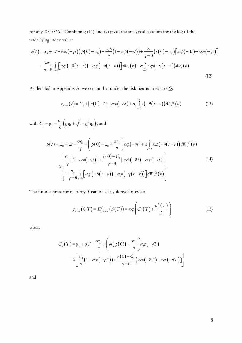
for any 0 t T . Combining (11) and (9) gives the analytical solution for the log of the
underlying index value:
0 0
0 0
μ λ λμ μ γ 0 μ 1 γ 0 μ δ γ
γ γ δ
λσδ γ σ γ
γ δ
rr
t tr
r sv v
p t t exp t p exp t r exp t exp t
exp t v exp t v dW v exp t v dW v
(12)
As detailed in Appendix A, we obtain that under the risk neutral measure Q:
1 10
0 δ σ δt
Q
bi var r rv
r t C r C exp t e t v dW v
(13)
with 2
1 1 2
σμ ρη 1 ρ η
δ
rrC , and
1 10 0
0
11
0
ση σημ μ 0 μ γ σ γ
γ γ
01 γ δ γ
γ γ δλ
σδ γ
γ δ
tQ
sv
tQr
rv
p t t p exp t exp t v dW v
r CCexp t exp t exp t
.
exp t v exp t v dW v
(14)
The futures price for maturity T can be easily derived now as:
2
0 2
σ0
2
yQ
bi var ,bi varf ,T E S exp CT
T T
(15)
where
1 12 0
11
ση σημ μ 0 γ
γ γ
0λ 1 γ δ γ
γ γ δ
C T ln p exp T
r CCexp T exp T exp T
T
and

9
222
2
2 1 γ δ1 2γ1 2δλσσσ 1 2γ
2γ 2δ 2γ γ δγ δ
1 γ δ 1 2γ2ρλσσ
γ δ γ δ 2γ
ry
r
exp Texp Texp Texp T
exp T ex T
T
p
The expression for the correlation of τ-period returns τ 1 τ 2bi varcorr r t ,r t for any 1 2 and τt , t ,
such that 1 2 τt t , is more involved and thus excluded here. However, it can be shown that for
certain values of the model parameters, the bivariate model, unlike the univariate model outlined
above, is more flexible and can allow for both positive and negative autocorrelations.
3. Data and Testing Methodology
For our empirical analysis of the differences between the forward and futures prices on the IPD7
UK property index we perform two types of tests. Firstly, we investigate whether the observed
difference between the forward and futures prices is statistically different from zero. Secondly,
we test which of a number of established continuous time models combined with various
methods of estimation is able to best capture this difference. Using the previously defined
notation, we have: n = 5 different maturities and N = 71 daily observations for each maturity.
3.1 Data
The data needed for our study contains IPD property futures prices, the IPD total return swap
(TRS) rates, the IPD index, and also the GBP interest rates needed to calculate discount factors.
Futures prices have been obtained from the European Exchange (Eurex8), the property TRS data
(the fixed rate) has been provided by Tradition Group, a major dealer on this market and the
IPD index was sourced from the Investment Property Databank (IPD9). In addition, the UK’s
interest rates have been downloaded from Datastream. Due to the availability of the property
futures and TRS data, the sample period used is daily from 4 February 2009 until 7 July 2009. It
generates 71 property futures daily curves and 71 sets of TRS rates with up to five years maturity
(the first maturity date is 31 December 2009, the second maturity date is 31 December 2010, the
7IPD stands for Investment Property Databank. A detailed description of the data is given in Section 3.1 below. 8 See www.eurexchange.com for more information on Eurex. IPD UK futures contracts started on 4 February 2009. 9 See www.ipd.com for more information on IPD.

10
third maturity date is 31 December 2011, the fourth maturity date is 31 December 2012, and the
fifth maturity date is 31 December 2013).
The evolution of the TRS series is depicted in Figure 1 and we could see that, for our period of
investigation, most of the IPD TRS rates are negative for the first, second, and third maturity
dates. For the fourth and fifth maturity dates, the values are higher or mostly positive. In
addition, there is a dramatic increase of the fixed rate at the end of February 2009, possibly due
to the rollover off the futures contracts in March combined with the publication of the IPD
index for the year ending in December 2008. The property futures prices are illustrated in Figure
2. The property futures prices are quoted on a total return basis.
INSERT FIGURE 1 HERE
INSERT FIGURE 2 HERE
The descriptive statistics of the TRS rates are reported in Table 1. The mean values are mostly
negative; the mean for the first maturity date is -17.80% and the means are increasing with
maturity. The excess kurtosis is negative for all five futures contracts and the first year TRS
contract and it is positive for the remaining four series of TRS rates. The skewness values have
negative signs, except for the four year futures contract, implying that the distributions of the
data are skewed to the left.
INSERT TABLE 1 HERE
It could be seen in Table 1 that the futures contract for the fifth maturity date appears to have
the highest mean. The highest standard deviation is showed in the futures contract for the
second maturity date. Similarly to TRS data, futures prices exhibit skewness and fat tails
characteristics.
From the daily TRS prices for the market five yearly maturities one can reverse engineer the
equivalent no-arbitrage forward prices for the same maturities. The equivalent fair property
forward prices are derived daily from 4 February until 7 July 2009, with maturities matching the
futures contracts maturities. The final engineered fair prices of property forwards are illustrated
in Figure 3. The descriptive moments of the differences between forward and futures prices on
IPD commercial index are also provided in Table 1. On average, the differences for the first
three maturities are positive, while for the fourth and fifth maturities they are negative.
INSERT FIGURE 3 HERE

11
3.2 Testing Methodology
First, we test whether the difference between the market TRS equivalent forward prices and
market futures prices is significantly different from zero. If this hypothesis is rejected, then in the
second stage a series of models and estimation methods are employed for the terms on the right
hand side of the fundamental relationship given by (1). The aim in the second stage is to decide
on the capability of various models to appropriately capture the dynamics of the index S and the
discount factor D.
For the first stage analysis, we run the following regression model for each maturity date Ti,
1 2 5i , , ..., :
0 0α β εi i i i tiF t ,T f t ,T (16)
(with Ti fixed for each of the five time series regressions) and test whether α0i = 0 and β0i =1. If
this null hypothesis cannot be rejected, then one can conclude that the difference between
forward and futures prices is due to noise. If, however, the null is rejected, we then proceed to
the second stage of our analysis. The same econometric analysis described above from a times
series point of view, can also be performed using panel data. Using panel data has a series of
advantages.10 Firstly, it enables the analysis of a larger spectrum of problems that could not be
tackled with cross-sectional or time series information alone. Secondly, it generally results in a
greater number of degrees of freedom and a reduction in the collinearity among explanatory
variables, thus increasing the efficiency of estimation. Furthermore, the larger number of
observations can also help alleviate model identification or omitted variable problems.
The regression equation in (16) is rewritten for our panel data as:
0 0α β εi i tiF t ,T f t ,T (17)
with 1 2 5i , , ..., and 1 2 71t , , ..., . More variations of a panel regression exist, the simplest
one being the pooled regression, described above in (17), which implies estimating the regression
equation by simply stacking all the data together, for both the explained and explanatory
variables. Furthermore, the fixed effects model for panel data is given by:
0 0α β α υi i i itF t ,T f t ,T (18)
10 See also Baltagi (1995), Hsiao (2003).

12
where αi varies cross-sectionally (i.e. in our case it is different for each maturity date Ti), but not
over time. Similarly, a time-fixed effects model can be formulated, in which case one would need
to estimate:
0 0α β λ υi i t itF t ,T f t ,T (19)
where λt varies over time, but not cross-sectionally. The fixed effects model and the time-fixed
effects model, as well as a model with both fixed effects and the time-fixed effects, will be
analysed. One can test whether the fixed effects are necessary using the redundant fixed effects
LR test.
For the panel data random effects model the regression specification is given by:
0 0α β ε υi i i itF t ,T f t ,T (20)
where εi is now assumed to be random, with zero mean and constant variance 2
εσ , independent
of υ it and if t ,T . Similarly, a random time-effects model can be formulated in the context of
this paper as:
0 0α β ε υi i t itF t ,T f t ,T (21)
Again, random effects and random time-effects models, as well as a two-way model which allows
for both random effects and random time-effects, can be estimated. Furthermore, it is important
to test whether the assumption that the random effects are uncorrelated with the regressors is
satisfied.
For the second stage analysis we shall employ several models for the dynamics of the IPD index
S. If the analysis is conditioned on knowing the bond prices, the RHS of identity (1) can be
expressed as:
Q
t Q
tQ
t
cov S T ,D t ,T S tE S T
E D t ,T B t ,T (22)
Based on (1) and (22), it is evident that for our testing purposes the following regression is
useful:

13
α β
m
Q
t ,m t ,m
f t ,T
S tF t ,T f t ,T E S T u
B t ,T
(23)
and test whether α = 0 and β =1, for each model m. For each model m, failing to reject the null
hypothesis implies that this particular model is suitable for describing the dynamics of the
underlying IPD index.
For a more comprehensive insight, we also consider a model for the interest rates that will lead
to stochastic discount factors. In this paper, we assume a Vasicek one-factor model that is
employed in conjunction with all models for the IPD index. Under this set-up we run the
following regression:
α β
Q
t ,m
t ,mQ
t ,m
cov S T ,D t ,TF t ,T f t ,T u
E D t ,T (24)
where again m is the model index, and the test whether α = 0 and β = 1 is for each model m. If
we fail to reject the null hypothesis, we then conclude that the model in question is suitable for
describing the dynamics of S and D.
Upon estimation of the model parameters, including the market price of risk (vector) η, as
described in previous sections, we can fit the regressions given in (23) and (24). The competing
models and methods of estimation are compared with respect to whether β is significant and
also considering the R2 measure of goodness-of-fit.
4. Calibration of the models
In order to be able to use the models enumerated in the preceding section we have to first
calibrate their parameters. The parameters of the continuous time models specified in (3) and
(11)-(12) can be estimated from the monthly log prices on the IPD index, observed over the
period between December 1986 and January 2009, and totalling 266 historical observations. The
estimates then will be carried forward for analysing the differences between the forward and
futures on IPD starting from February 2009.

14
4.1 Maximum Likelihood Estimation
When feasible, parametric inference for diffusion processes from discrete-time observations
should employ the likelihood function, given its generality and desirable asymptotic properties of
consistency and efficiency (Phillips and Yu, 2009). The continuous time likelihood function can
be approximated with a function derived from discrete-time observations, obtained by replacing
the Lebesgue and Ito integrals with Riemann-Ito sums. Remark that this approach gives reliable
results only when the observations are spaced at small time intervals. When the time between
observations is not small the maximum likelihood estimator can be strongly (upward) biased in
finite samples.11
We first de-trend the log price data by estimating the regression:
0μ μk kt k tp t u (25)
and subsequently work with the residuals from this equation, where k = 1, 2, …, 266 and
τkt k , with 1
τ12
for monthly returns.
The (exact) discretization of equation (3) leads to:
1
εk k kt t tu cu (26)
where γτc exp and
1
ε σ γk
k
k
t
t kt
exp t s dW s ;
2σε 0 1 2γτ
2γktN , exp .
Maximum likelihood estimation of the discrete-time model in (26) gives12 0 995086c . and the
standard deviation of εktas 0.011.
The exact discretization of the two-factor model given by (11)-(12) is:
1 1
1
α β φ ε
α β ε
k k k k
k k k
t q q t t q ,t
t r r t r ,t
q q r
r r (27)
11 Further discussion is given in Dacunha-Castelle and Florens-Zmirou (1986), Lo (1988), Florens-Zmirou(1989), Yoshida(1990) and Phillips and Yu (2009) 12 To check the stability of the parameter estimates, the estimation above is repeated using a larger sample, namely Dec 1986 to Oct 2010, with an increased sample size of 287 monthly observations. The parameter estimates do not change much.

15
where, for reasons of space, the expressions for the parameters as well as the distribution of the
error terms in (27) are only given in Appendix B.
4.2 Alternative estimation methods: Martingale estimation and Markov Chain Monte Carlo (MCMC)
Lo (1988) argued that maximum likelihood estimation does not produce consistent estimates for
the parameters of the continuous time model, when a discrete data sample is used. Two
alternative estimation techniques that are applied here in order to circumvent this problem are
the martingale estimation method described in Bibby & Sorensen (1995) and Markov Chain
Monte Carlo (MCMC) methodology (see Tsay, 2008).
Bibby and Sorensen (1995) have overcome this difficulty by developing a martingale estimating
function estimator. A consistent estimator cannot be obtained from the discrete approximation
of the likelihood function L because the associated pseudo-score function is biased. This bias is
directly related to the time between observations being sizeable. The methodology proposed by
Bibby and Sorensen (1995) – briefly described in Appendix D- compensates the pseudo-score
function in order to obtain a martingale. Their estimator is consistent and asymptotically normal.
Following example 2.1 in Bibby and Sorensen (1995) and using previously defined notation, the
estimator resulting from the martingale estimating function for the mean reversion parameter γ
is:
1
1
266
1
2662
1
1γ
τ
k k
k
t tk
tk
q qln
q
provided that the numerator is positive. It can be shown that this estimator is equal to the
maximum likelihood estimator for the case when the volatility parameter σ is known.
Since the martingale approach is not suitable for deterministic time trending processes, we only
apply it for models mean reverting towards a constant threshold. The parameters obtained with
this method are 0μ 0.3382 γ 0.0443 σ 0 01. . These values will feed into formula (8) and lead
to model futures prices.
MCMC techniques13 are based on a Bayesian inference theoretical support and offer an elegant
solution to many problems encountered with other estimation methods, at the cost of
computational effort. The main advantage of employing this type of inferential mechanism is the
13 For an excellent introduction see Tsay (2010). All MCMC inference in this paper has been produced with WinBUGS 1.4, from a sample of 100,000 iterations after a burn-in period of 500000 iterations.

16
capability to produce not only a point estimate but an entire posterior distribution for parameters
of interest. Selecting various statistics from this distribution provides a more informed view on
the plausible values of the parameters. Hence, for estimation purposes we select the mean, the
2.5% quantile and the 97.5% quantile of the posterior distribution of the mean reversion
parameter. The estimates for the discretized version of the mean-reverting model given in (5) are
reported in Table 3. One great advantage of the MCMC approach is that all parameters are
estimated easily from the same output without additional computational effort.
4.3 The Calibration of the Market Price of Risk
To calibrate the market price of risk η, we follow standard practice and minimize the mean
squared error function; for the univariate model we have:
5 2
1η
η ηt
*
t i univ t iiR
arg min f t ,T f , t ,T
(28)
where if t ,T represents the market futures price and ηuniv t if , t ,T is the theoretical futures
price at time t for maturity iT . This optimization exercise is performed for each day in our
sample and for each of the estimation methodologies described above. The resulting time series
for the market price of risk, for each set of estimates are given in Figure 4.14
INSERT FIGURE 4 HERE
All parameter estimates can be determined now and then the theoretical model can be used for
producing property futures prices.
For the bivariate model, to calibrate the market price of risk vector 1 2η η 'η , we solve:
2
5 2
1
ηi bi var t iiR
arg min t ,T , t ,T
η
ηt
t g g (29)
where '
i i it ,T f t ,T r t ,Tg are the observed futures prices and the interest rates
obtained from observable bond prices, respectively. For clarity,
14 For the ML estimation we also investigate the calibration of a surface for the market price of risk, where we now allow η to vary across maturities as well as across time. The results are depicted in Figure 5.
17
ηbi var t i bi var i bi var i, t ,T f t ,T r t ,T 'g are their model counterparts, as given in (15) and
(13), respectively.
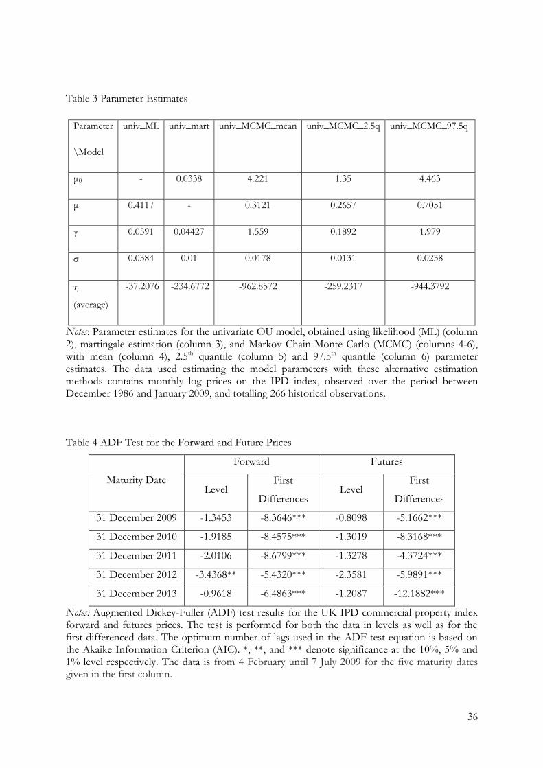
Table 2 gives a list of the models investigated in this paper with various methods of estimation.
In Table 3 we report the parameter estimation results for these models based on our data.
INSERT TABLE 2 HERE
INSERT TABLE 3 HERE
5. Empirical Analysis
Our empirical analysis is divided into a part related to plain tests of the market differences
between forward and futures prices on IPD index and a more refined analysis looking at several
models for the underlying IPD index dynamics, coupled with a model for interest rates, but also
considering several estimation methods.
5.1 Model-free analysis
Having available both series of forward and futures prices allows us to test directly whether the
forward – futures difference time series diverges significantly away from zero.
Before running the time-series regressions in (17-22) we test whether the forward and futures
price series are stationary using the Augmented Dickey-Fuller (ADF) test. The results are
reported in Table 4.
INSERT TABLE 4 HERE
As we could see from the Table 4, most of the ADF results show that the forward series for the
first, second, third, and fifth maturity dates are non-stationary while the forward series for the
fourth maturity date is stationary at 5% significance level. In addition, the ADF test indicates that
the futures series for all maturity dates are non-stationary. Furthermore, we also investigated the
stationarity of the first differenced data. According to Table 4, the forward and futures series for
all maturity dates are stationary in the first differences.
Since most of the data is found to be non-stationary in levels and stationary in the first
differences, we perform the remaining analysis on the first differenced data. We test H0: α0i = 0
and β0i =1 vs. H1: α0i≠ 0 or β0i≠1, using an F-test and the results could be found in the Table 5.
INSERT TABLE 5 HERE
18
The F-test results presented in Table 5 show that the null hypothesis for all maturity dates could
be rejected at 1% significance level. We could conclude that the difference between forward and
futures is not just a noise. 15 The same conclusion is reached if we analyse the values of the t-
statistics for the forward-futures differences reported in Table 6.
INSERT TABLE 6 HERE
Panel Stationarity tests
Levin and Lin (1993), Levin, Lin and Chu (2002), Im, Pesaran and Shin (1997) and Maddala and
Wu (1999) have developed unit root tests for panel data16. The results of these tests are reported
in Table 7.
INSERT TABLE 7 HERE
As it was the case with the time series data, the panel data is non-stationary in the levels,
however, the first differenced data is stationary and hence we continue our analysis using the first
differences. To choose an appropriate specification for our panel regression, we first test
whether the fixed effects are necessary using the redundant fixed effects LR test. The results of
this test are reported in Table 8.
INSERT TABLE 8 HERE
From the test results reported in Table 8, it appears that a model with fixed time effects only is
most supported by our data. Furthermore, we also investigate whether a random effects model is
appropriate using the Hausman test; the results of this test are also reported in Table8.
Based on these results, we arrive at the conclusion that the random effect model is to be
preferred in this case.
Next, we compute the F-test statistic for multiple coefficient hypotheses using the panel
regression random effect specification; the results are reported in Table 9.
INSERT TABLE 9 HERE
15 In addition, we also investigate the diagnostic statistics for these regressions and report the Durbin-Watson test statistic results in Table 5. We note that for all but the fifth maturity date there is no autocorrelation in the regressions errors. 16 For a description of the tests, see Hsiao (2003), p. 298-301.

19
According to Table 9, we could see that the F-values are significant at 1% level. We could
strongly reject the null hypothesis (H0: α0 = 0 and β0 =1) and conclude that the differences
between forward and futures are not just noise in the panel data.17
5.2 Model-based analysis18
From a financial economics point of view, it has been established that even if the interest rates
are constant then futures prices can differ from the associated forward prices. Assuming that
interest rates are stochastic leads directly to the conclusion that the two series will diverge
significantly over time. In this paper we would like to pose and answer the question, “which
model and estimation method” most likely support the observed market differences.
Furthermore, an additional level of complexity is generated from employing panel data tests.
Tables 10 and 11 summarize the results of our model comparison, for the time series and panel
data, respectively. The martingale method and the MCMC methods perform better than the ML
method. The R-square seems to increase with maturity overall hinting that stationarity problems
may be more acute for near maturities. Please note that since maturities are fixed in the calendar
by the market, the time to maturity of our series gets progressively smaller, across all five
contracts.
INSERT TABLE 10 HERE
INSERT TABLE 11 HERE
Our results in Table 11 reveal that for panel data analysis all models employed here are well
specified and the beta t-test is highly significant. The univariate model coupled with maximum
likelihood estimation is by far the best approach, the R-squared being close to 93%.
6. Conclusions
In this paper we analyse the differences between forward and futures prices on a new asset class,
commercial real-estate, using a battery of models, estimation methods and tests. The forward
prices have been reversed engineered from total return swap rates using standard market
practice. Testing is done on individual time series data but also in a panel data framework.
17 In addition, the values of Durbin Watson test show that there is no autocorrelation in the panel regression errors. 18 The futures and engineered forward prices are given as percentages of the underlying IPD index S(t). In order to be able to conduct the testing in this section, we need to first obtain the transformed futures and forward prices as
follows:
100i i
S tf t ,T f t ,T and
100
i i
S tF t ,T F t ,T .

20
Our results provide evidence of significant differences between the implied forward and futures
prices for the IPD UK index. One possible explanation could be the period of study, several
months during 2009, in the aftermath of the subprime crisis.
Although our overall conclusion is that, for the period 4 February 2009 to 7 July 2009, the
forward prices were different from futures prices, there is substantial variation in the strength of
these results across contract maturities, methods of estimation and testing frameworks. Given
the significance of our results even on a model-free basis, we organised a model race that best
explains the relationship between synthetic forward prices derived from daily total return swap
rates and the daily futures prices. The models were generated from using various methods of
estimation for the mean-reverting OU continuous time process assumed for the underlying IPD
index. Our models provided significant explanatory power for the relationship between forward
and futures prices on commercial real-estate index in UK but the analysis of the error terms
shows that there is more that can be explained. From a theoretical point of view our study can
be expanded to two-factor models as detailed in the paper. Unfortunately, due to lack of space
we could not report also the results from the two-factor models subset, but we hope to do that
in the very near future.
21
Appendices
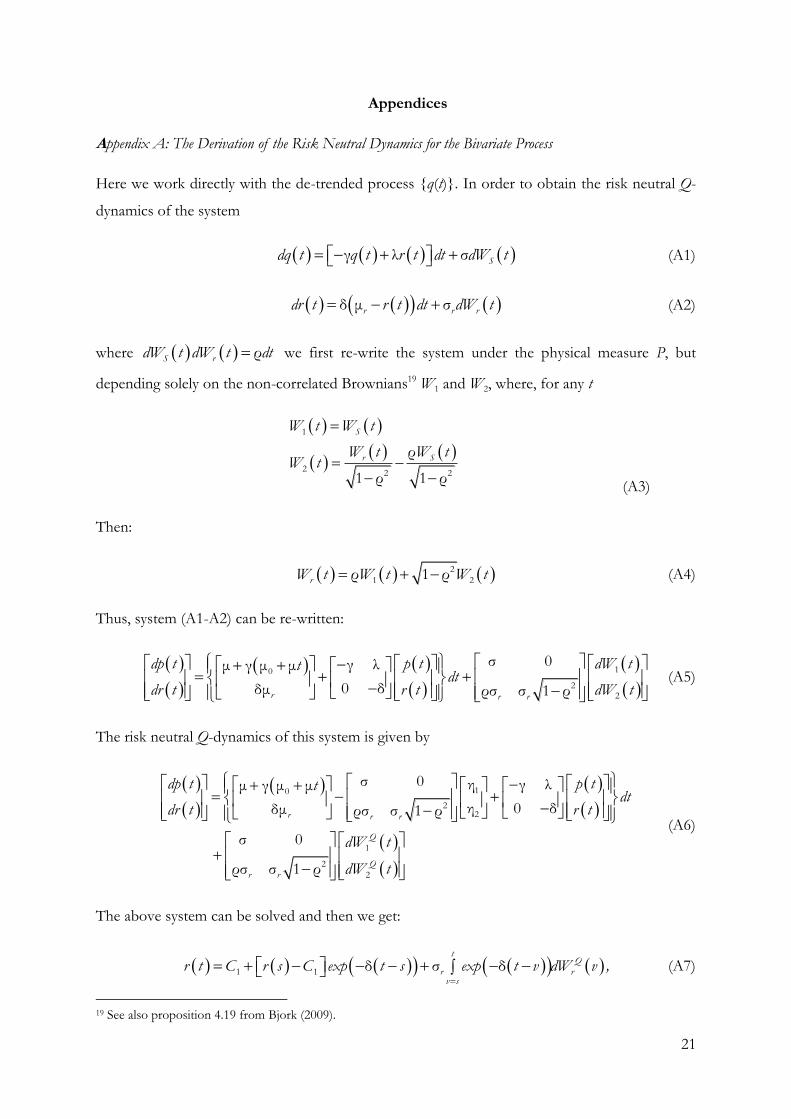
Appendix A: The Derivation of the Risk Neutral Dynamics for the Bivariate Process
Here we work directly with the de-trended process {q(t)}. In order to obtain the risk neutral Q-
dynamics of the system
γ λ σ Sdq t q t r t dt dW t (A1)
δ μ σr r rdr t r t dt dW t (A2)
where ρS rdW t dW t dt we first re-write the system under the physical measure P, but
depending solely on the non-correlated Brownians19 W1 and W2, where, for any t
1
22 2
ρ
1 ρ 1 ρ
S
r S
W t W t
W t W tW t
(A3)
Then:
2
1 2ρ 1 ρrW t W t W t (A4)
Thus, system (A1-A2) can be re-written:
10
22
σ 0γ λμ γ μ μ
0 δδμ ρσ σ 1 ρr r r
dp t p t dW ttdt
dr t r t dW t
(A5)
The risk neutral Q-dynamics of this system is given by
10
22
1
2
2
σ 0 η γ λμ γ μ μ
η 0 δδμ ρσ σ 1 ρ
σ 0
ρσ σ 1 ρ
r r r
Q
Q
r r
dp t p ttdt
dr t r t
dW t
dW t
(A6)
The above system can be solved and then we get:
1 1 δ σ δt
Q
r rv s
r t C r s C exp t s exp t v dW v , (A7)
19 See also proposition 4.19 from Bjork (2009).

22
with 2
1 1 2
σμ ρη 1 ρ η
δ
rrC , and 2
1 2ρ 1 ρQ Q Q
rdW t W t W t .
Appendix B: The Discretization of the Bivariate Model
The complete specification of the discretization for the two-factor model used in the paper is
given as
1 1
1
α β φ ε
α β ε
k k k k
k k k
t q q t t q ,t
t r r t r ,t
q q r
r r (B1)
where
1 γτ δτ γτα μ λ β γτ
γ γ δ
λφ δτ γτ α μ 1 δτ β δτ
γ δ
q r q
r r r
exp exp exp, exp ,
exp exp ; exp , exp ,
1 1
λσε δ γ σ γ
γ δ
k k
k
k k
t tr
q ,t k k r k st t
exp t s exp t s dW s exp t s dW s
1
ε σ δk
k
k
t
r ,t r k rt
exp t s dW s .
We also notice that:
λ
α α μ φγ
q r r
(B2)
The error vector is bivariate normal, with covariance matrix:20
ε ε ε
ε ε ε
k k k
k k k
q ,t q ,t r ,t
q ,t r ,t r ,t
var cov ,
cov , var
20 Lo and Wong (1995) obtained the same error covariance matrix although their model is not the same as ours.

23
where:
22
2
2 1 γ δ τ1 2γτ1 2δτλσσε 1 2γτ
2γ 2δ 2γ γ δγ δ
1 γ δ τ 1 2γτ2ρλσσ
γ δ γ δ 2γ
k
rq ,t
r
expexpexpvar exp
exp exp
(B3)
2σ
ε 1 2δτ2δk
rr :tvar exp
(B4)
2 1 γ δ τ1 2δτλσ ρσσε ε 1 γ δ τ
γ δ 2δ γ δ γ δk k
r rq ,t r ,t
expexpcov , exp
(B5)
(B3) and (B5) represent a system of two equations in two unknowns, σ and ρ.
Appendix C: Maximum Likelihood Estimation - Continuous Time Models Parameters in terms of the Discrete
Time Models Parameters
Univariate Model
ε
2γγ σ σ
τ 1 2γτ tk
ln c;
exp
(C1)
Bivariate Model
ε
β
β ββ φ 2δγ δ λ σ σ
τ τ τ β β 1 2δτ r ,tk
r
q qr
r
r q
lnln ln
; ; ;exp
(C2)

24
Appendix D: Martingale Estimation
If 2 nX , X ,..., X is a discrete observation sample from the path of the diffusion
φ σ φdX t b X t , dt X t , dW t (D1)
where φ is a parameter vector.
Then, denoting φ 0φF x, E X |X x , Bibby and Sorensen (1995) build the estimating
function
1
121
1
φ
φφ φ
σ φ
( i )
i n
n i ( i )i
( i )
b X ,
G X F X ,X ,
(D2)
This is a zero-mean martingale and thus it does not matter whether the diffusion coefficient σ
depends on the parameter or not.

25
References
Allen, L., Thurston, T., 1988. Cash-Futures Arbitrage and Forward-Futures Spreads in the
Treasury Bill Market. Journal of Futures Markets 8 (5), 563-573.
Alles, L.A., Peace, P.P.K., 2001. Futures and forward price differential and the effect of marking-
to-market: Australian evidence. Accounting and Finance 41, 1-24.
Amerio, E., 2005. Forward Prices and Futures Prices: A Note on a Convexity Drift Adjustment.
Journal of Alternative Investment. Fall, 80-86.
Baltagi, B.H. (1995). Econometric Analysis of Panel Data. John Wiley, Chichester, UK.
Bibby, B. M., Sorensen, M., 1995. Martingale Estimation Functions for Discretely Observed
Diffusion Processes. Bernoulli 1(1/2), 17-39.
Bjork, T., 2009. Arbitrage Theory in Continuous Time, 3rd Edition, Oxford University Press, Oxford,
UK.
Case, K. E., Shiller, R. J., 1989. The efficiency of the market for single family homes. American
Economic Review 79, 125-37.
Case, K. E., Shiller, R. J., 1990. Forecasting prices and excess returns in the housing market.
AREUEA Journal 18, 253-73.
Case, K. E., Shiller, R. J., 1996. Mortgage default risk and real estate prices: the use of index
based futures and options in real estate. Journal of Housing Research 7, 243-58.
Case, K. E., Shiller, R.J., Weiss, A.N., 1993. Index-Based futures and options trading in real
estate. Journal of Portfolio Management 19, 83-92.
Chang, C.W., Chang, J.S.K., 1990. Forward and Futures Prices: Evidence from the Foreign
Exchange Markets. Journal of Finance. 45 (4), 1333-1336.
Cornell, B., Reinganum, M.R., 1981. Forward and Futures Prices: Evidence from the Foreign
Exchange Markets. Journal of Finance 36 (12), 1035-1045.
Cox, J.C., Ingersoll, J.E., Ross, S.A., 1981. The Relation between Forward Prices and Futures
Prices. Journal of Financial Economics 9, 321-346.

26
Dacunha-Castelle, D., Florens-Zmirou, D., 1986. Estimation of the coefficients of a diffusion
from discrete observations. Stochastics 19, 263-284.
Florens-Zmirou, D., 1989. Approximate discrete-time schemes for statistics of diffusion
processes. Statistics 20(4), 547-557.
Dezhbakhsh, H., 1994. Foreign Exchange Forward and Futures Prices: Are They Equal? Journal
of Financial and Quantitative Analysis 29(1), 75-87.
Fabozzi, F.J., Shiller, R., Tunaru, R.S., 2011. A Pricing Framework for Real-Estate Derivatives,
European Financial Management, forthcoming.
Fisher, J. D., 2005. New Strategies for Commercial Real Estate Investment and Risk
Management. Journal of Portfolio Management 32, 154-161.
French, K.R., 1983. A Comparison of Futures and Forward Prices. Journal of Financial Economics
12, 311-342.
Fried, J., 1994. U.S. Treasury Bill Forward and Futures Prices. Journal of Money, Credit and Banking.
26(1), 55-71.
Greene, W.H., 2011. Econometric Analysis, 7th Edition, Pearson.
Grinblatt, M., Jegadeesh, N., 1996. Relative Pricing of Eurodollar Futures and Forward
Contracts. Journal of Finance 51(4), 1499-1522.
Hamilton, J.D., 1994. Time Series Analysis, Princeton University Press.
Hsiao, C., 2003. Analysis of Panel Data, 2nd Edition. Cambridge University Press, Cambridge, UK.
Im, K.S., Pesaran, M.H., Shin, Y., 2003. Testing for Unit Roots in Heterogeneous Panels. Journal
of Econometrics 115(1), 53-74.
Jarrow, R.A., Oldfield, G.S., 1981. Forward and Futures Contracts. Journal of Financial Economics 9,
373-382.
Kane, E.J., 1980. Market Incompleteness and Divergences between Forward and Futures
Interest Rates. Journal of Finance 35(2), 221-234.
Kwiatkowski, D., Philips, P., Schmidt, P., Shin, Y., 1992. Testing the Null Hypothesis of
Stationarity Against the Alternative of a Unit Root. Journal of Econometrics 54, 159-178.

27
Levin, A., Lin, C., 1993. Unit Root Tests in Panel Data: Asymptotic and Finite Sample
Properties. Mimeo. University of California, San Diego.
Levin, A., Lin, C., Chu, J., 2002. Unit Root Tests in Panel Data: Asymptotic and Finite Sample
Properties. Journal of Econometrics 108(1), 1-24.
Levy, A., 1989. A Note on the Relationship between Forward and Futures Contracts. Journal of
Futures Markets 9(2), 171-173.
Lo, A.W., 1988. Maximum Likelihood Estimation of Generalized Ito Processes with Discretely
Sampled Data. Econometric Theory 4 (2), 231-247.
Lo, A. W., Wang, J., 1995. Implementing Option Pricing Models when Asset Returns are
Predictable. Journal of Finance. 50(1), 87-129.
Maddala, G.S., Wu, S., 1999. A Comparative Study of Unit Root Tests with Panel Data and a
New Simple Test. Oxford Bulletin of Economics and Statistics 61, 631-652.
Margrabe, W., 1978. A Theory of Forward and Futures Prices. Unpublished Working Paper (The
Warton School, University of Pennsylvania, Philadelphia, PA.
Morgan, G., 1981. Forward and Futures Pricing of Treasury Bills. Journal of Banking and Finance. 5,
483-496.
Meulbroek, L., 1992. A Comparison of Forward and Futures Prices of an Interest Rate-Sensitive
Financial Asset. Journal of Finance 47(1), 381-396.
Park, H.Y., Chen, A.H., 1985. Differences between Futures and Forward Prices: A Further
Investigation of the Marking-to-Market Effects. Journal of Futures Markets 5(1), 77-88.
Phillips, P.C. B., Yu, J., 2009. Maximum Likelihood and Gaussian estimation of Continuous
Time Models in Finance in Handbook of Financial Time Series, Andersen, T.G., Davis, R.A.,
Mikosch, T. (Eds.)
Polakoff, M., 1991. A Note on the Role of Futures Indivisibility: Reconciling the Theoretical
Literature. Journal of Futures Markets 11, 117-120.
Polakoff, M., Diaz, F., 1992. The Theoretical Source of Autocorrelation in Forward and Futures
Price Relationships. Journal of Futures Markets 12 (4), 459-473.

28
Richard, S., Sundaresan, M., 1981. A Continuous Time Equilibrium Model of forward Prices and
Futures Prices in Multigood Economy. Journal of Financial Economics 9, 347-392.
Schwartz, E.S., 1997. The Stochastic Behavior of Commodity Prices: Implications for Valuation
and Hedging. Journal of Finance 52 (3), 923-973.
Shiller, R. J., 2008. Derivatives Markets for Home Prices, Yale Economics Department Working
Paper No. 46, Cowles Foundation Discussion Paper No. 1648.
Shiller, R. J., Weiss, A. N., 1999. Home equity insurance. Journal of Real Estate Finance and
Economics 19, 21-47.
Shreve, S.E., 2004. Stochastic Calculus for Finance II: Continuous-Time Models. Springer Finance.
Tsay, R., 2010. Analysis of Financial Time Series, 3rd Edition, Wiley-Interscience.
Viswanath, P.V., 1989. Taxes and the Futures-Forward Price Difference in the 91-Day T-Bill
Market. Journal of Money, Credit and Banking 21(2), 190-205.
Wimshculte, J., 2010. The Futures and Forward Price Differential in the Nordic Electricity
Market. Energy Policy 38, 4731-4733.
Yoshida, N., 1990. Estimation for diffusion processes from discrete observations. Journal of
Multivariate Analysis 41, 220-242.

29
Figure 1 IPD Total Return Swap Rates (mid prices)
Notes: The plotted data is from 4 February until 7 July 2009 for the five maturity dates fixed in the market calendar, for the period of study. The total return swap rates are given as a fixed rate and not as a spread over Libor. A negative total return swap rate implies that the underlying commercial property market will depreciate over the period to the horizon indicated by the maturity of the contract.
-23.00%
-18.00%
-13.00%
-8.00%
-3.00%
2.00%
Maturity Date 31-Dec-09
Maturity Date 31-Dec-10
Maturity Date 31-Dec-11
Maturity Date 31-Dec-12
Maturity Date 31-Dec-13

30
Figure 2 Eurex Futures Prices
Notes: The plotted data is from 4 February until 7 July 2009 for the five maturity dates fixed in the market calendar. Futures prices are given on a total return basis so a futures price of 110 for December 2012 implies that the market expects a 10% appreciation of the commercial property in UK at this horizon.
70.00
80.00
90.00
100.00
110.00
120.00
Maturity Date 31-Dec-09
Maturity Date 31-Dec-10
Maturity Date 31-Dec-11
Maturity Date 31-Dec-12
Maturity Date 31-Dec-13

31
Figure 3 The Fair Prices of Property Forwards
Notes: The plotted data is from 4 February until 7 July 2009 for the five maturity dates fixed in the market calendar, for the period of study. The fair property forward prices are reversed engineered from the corresponding portfolio of total return swaps.
75
80
85
90
95
100
105
110
115
Maturity Date 31-Dec-09
Maturity Date 31-Dec-10
Maturity Date 31-Dec-11
Maturity Date 31-Dec-12
Maturity Date 31-Dec-13

32
Figure 4 Market Price of Risk
Notes: The figure plots the market price of risk for IPD commercial property index under the univariate OU model, with underlying model parameters estimated using maximum likelihood (ML) in panel (a), martingale estimation in panel (b), and Markov Chain Monte Carlo (MCMC) in panels (c)-(e), with posterior mean (panel c), posterior 2.5th quantile (panel d) and posterior 97.5th quantile (panel e) parameter estimates, using monthly log prices on the IPD index, observed over the period between December 1986 and January 2009. The market price of risk is fitted by minimising the mean squared error function, which measures the mean squared distance between the market and model futures prices, for each of the 71 days in the sample and across the five futures maturities. The IPD futures data is from 4 February until 7 July 2009, for the five maturities, namely December 2009, December 2010, December 2011, December 2012 and December 2013.

33
Figure 5 Market Price of Risk
Notes: The figure plots the market price of risk surface for IPD commercial property index and
for the univariate OU model, with underlying parameters estimated using maximum likelihood
(ML), using monthly log prices on the IPD index, observed over the period between December
1986 and January 2009. The market price of risk is fitted by minimising the mean squared error
function, which measures the mean squared distance between the market and model futures
prices, for each of the 71 days in the sample and each of the five futures maturities. The market
price of risk is thus assumed vary both across time and across futures contracts maturities. The
IPD futures data is from 4 February until 7 July 2009 for the five maturities, namely December
2009, December 2010, December 2011, December 2012 and December 2013.

34
Table 1. Descriptive Statistics for total return swap rates, Eurex futures prices and the forward-
futures differences.
Maturity Dates
31-Dec-09 31-Dec-10 31-Dec-11 31-Dec-12 31-Dec-13
Total Return Swaps
Mean -0.178 -0.0971 -0.0389 -0.0056 0.0138
standard deviation 0.0217 0.0548 0.0521 0.0401 0.0336
Skewness -0.6925 -1.3581 -1.4446 -1.4177 -1.3889
Kurtosis -0.5131 0.1383 0.2633 0.2135 0.1585
Futures prices
Mean 81.1982 94.275 106.1732 111.7035 113.5915
standard deviation 2.6558 10.6358 5.1369 1.2792 3.7762
Skewness -0.0992 -0.4889 -0.5411 0.164 -0.2771
Kurtosis -1.5313 -1.7844 -1.6426 -0.6302 -1.6544
Forward – Futures Differences
Mean 1.1018 4.2432 2.0765 -1.599 -3.7103
Standard Deviation 1.3846 7.2574 3.7344 1.0573 3.0863
Kurtosis 0.3093 0.9912 0.8006 0.0824 -1.6454
Skewness 1.2702 1.6562 1.5582 0.3179 0.2274
Notes: The descriptive statistics are of the total return swap rates, futures prices and forward-
futures differences on IPD UK All Property index. Daily mid prices are used for calculation for
the period 4 February 2009 to 7 July 2009 for the five market calendar maturities, namely
December 2009, December 2010, December 2011, December 2012 and December 2013. The
forward prices used here are the synthetic fair prices derived from total return swap rates,
synchronous with the futures prices.

35
Table 2 Models
Name Model Estimation method
univ_ML univariate time-trending OU:
γ σdq t q t dt dW t
exact maximum likelihood
univ_mart martingale estimation
univ_MCMC_mean Markov Chain Monte Carlo (MCMC), mean parameter estimates
univ_MCMC_2.5q MCMC, using the 2.5th quantile of the distribution of estimates
univ_MCMC_97.5q MCMC, using the 97.5th quantile of the distribution of estimates
bivar_ML bivariate time-trending OU:
γ λ σ
δ μ σ
ρ
S
r r r
S r
dq t q t r t dt dW t
dr t r t dt dW t
dW t dW t dt
exact maximum likelihood
biv_MCMC_mean MCMC, mean parameter estimates
biv_MCMC_2.5q MCMC, using the 2.5th quantile of the distribution of estimates
biv_MCMC_97.5q MCMC, using the 97.5th quantile of the distribution of estimates
Notes: q(t) is the de-trended log price process for the underlying S(t), the IPD UK commercial property price index: p t ln S t ;
0μ μp t q t t. r(t) denotes the short interest rate. For both models, the futures price is obtained as:
00 Q
m ,mf ,T E S Twhere m = univ
or bivar, for the two models, respectively, Q is the martingale pricing measure, and T is the futures maturity time.
36
Table 3 Parameter Estimates
Parameter
\Model
univ_ML univ_mart univ_MCMC_mean univ_MCMC_2.5q univ_MCMC_97.5q
μ0 - 0.0338 4.221 1.35 4.463
μ 0.4117 - 0.3121 0.2657 0.7051
γ 0.0591 0.04427 1.559 0.1892 1.979
σ 0.0384 0.01 0.0178 0.0131 0.0238
η
(average)
-37.2076 -234.6772 -962.8572 -259.2317 -944.3792
Notes: Parameter estimates for the univariate OU model, obtained using likelihood (ML) (column 2), martingale estimation (column 3), and Markov Chain Monte Carlo (MCMC) (columns 4-6), with mean (column 4), 2.5th quantile (column 5) and 97.5th quantile (column 6) parameter estimates. The data used estimating the model parameters with these alternative estimation methods contains monthly log prices on the IPD index, observed over the period between December 1986 and January 2009, and totalling 266 historical observations.
Table 4 ADF Test for the Forward and Future Prices
Maturity Date
Forward Futures
Level First
Differences Level
First
Differences
31 December 2009 -1.3453 -8.3646*** -0.8098 -5.1662***
31 December 2010 -1.9185 -8.4575*** -1.3019 -8.3168***
31 December 2011 -2.0106 -8.6799*** -1.3278 -4.3724***
31 December 2012 -3.4368** -5.4320*** -2.3581 -5.9891***
31 December 2013 -0.9618 -6.4863*** -1.2087 -12.1882***
Notes: Augmented Dickey-Fuller (ADF) test results for the UK IPD commercial property index forward and futures prices. The test is performed for both the data in levels as well as for the first differenced data. The optimum number of lags used in the ADF test equation is based on the Akaike Information Criterion (AIC). *, **, and *** denote significance at the 10%, 5% and 1% level respectively. The data is from 4 February until 7 July 2009 for the five maturity dates given in the first column.

37
Table 5 F-Test for Time Series Data
Maturity Date F-test Durbin-Watson
Statistic
31 December 2009 83.5072*** 1.9905
31 December 2010 49.4309*** 2.0595
31 December 2011 23.8320*** 2.0613
31 December 2012 31.1717*** 2.2589
31 December 2013 158.2534*** 2.7247
Notes: F-Test and Durbin Watson statistic results for the regression in the equation (16) for the property forward and futures data from 4 February until 7 July 2009 for the five maturity dates given in the first column. For the F-test, the null hypothesis is that the difference between the forward and futures prices is just noise (i.e. α0i = 0 and β0i =1). *, **, and *** denote significance at the 10%, 5% and 1% level respectively.
Table 6 T- statistics for the Differences between Forward and Futures prices
Maturity Dates
31-Dec-09 31-Dec-10 31-Dec-11 31-Dec-12 31-Dec-13
t-statistic 6.7060*** 4.9265*** 4.6852*** -12.741*** 10.1291***
Note: The values of the t-test are computed for the differences between forward and futures prices on the UK IPD commercial property index, using data from 4 February until 7 July 2009 for the five maturity dates given in the second row. *, **, and *** denote significance at the 10%, 5% and 1% level respectively.
Table 7 Panel Unit Root Tests
Method Forward Futures
Level First Differences Level First Differences
Levin, Lin & Chu t* -1.8292 -6.7737*** -0.7206 -4.0345***
Im, Pesaran & Shin
W-stat -1.1578 -10.4686*** 0.3880 -8.3918***
Note: Results for the panel unit root tests of Levin, Lin and Chu (2002) and Im, Pesaran and Shin (2003) for forward and futures price data on the UK IPD commercial property index, from 4 February until 7 July 2009 for five maturity months, namely December 2009, December 2010, December 2011, December 2012 and December 2013.*, **, and *** denote significance at the 10%, 5% and 1% level respectively

38
Table 8 Tests for determining the most suitable panel regression model
Test Value
Redundant Fixed Effects Test
Cross-section F 1.0925
Cross-section Chi-square 5.5181
Period F 2.2062***
Period Chi-square 154.1939***
Cross-Section/Period F 2.1450***
Cross-Section/Period Chi-square 157.7444***
Hansen Test
Cross-section random 3.0341*
Period random 0.0003
Cross-section and period random 0.1690
Notes: The redundant fixed cross-section effects test has a panel regression with fixed time (period) effects only under the null. Both the F and the chi-square version of the test are reported. The redundant fixed time (period) effects has a panel regression with fixed cross-section effects only under the null. Both the F and the chi-square version of the test are reported. For the random effects test (i.e. Hansen test) the null hypothesis in this case is that the random effect is uncorrelated with the explanatory variables. The panel data is from 4 February until 7 July 2009 for five maturities, namely December 2009, December 2010, December 2011, December 2012 and December 2013.*, **, and *** denote significance at the 10%, 5% and 1% level respectively.
Table 9 The F-test for Panel Data
Test Statistic Value
F-statistic 237.3960***
Durbin Watson Statistic 2.1419
Notes: F-test and Durbin Watson statistic results for the regression in the equation (20) for the property forward and futures panel data from 4 February until 7 July 2009, using the cross-section random effects specification. For the F-test, the null hypothesis is that the difference between the forward and futures prices is just noise (i.e. α0 = 0 and β0 =1).*, **, and *** denote significance at the 10%, 5% and 1% level respectively.

39
Table 10 Model Comparison – Time Series Data
Test\Model univ_ML univ_mart univ_MCMC_mean univ_MCMC_2.5q univ_MCMC_97.5q
1st Maturity
F-test 120757.2*** 122000.3*** 112810.4*** 121757.8*** 99747.38***
t-test for β 1.4369 1.607 -0.8494 1.5724 -1.9758*
R_squared 0.0291 0.0361 0.0103 0.0346 0.0535
2nd Maturity
F-test 5946.6*** 6108.451*** 2705.565*** 6043.822*** 411.4135***
t-test for β 2.0079** 2.1145** 0.5759 2.0585** 0.5991
R_squared 0.0552 0.0608 0.0048 0.0579 0.0052
3rd Maturity
F-test 30397.9*** 36595.58*** 4200.665*** 31643.03*** 63.6275***
t-test for β t-
test for β
4.2573*** 5.1767*** 4.2845*** 4.3118*** 15.7831***
R_squared 0.208 0.2797 0.2101 0.2123 0.7831
4th Maturity
F-test 216988.5*** 360635.3*** 2426.505*** 214077.2*** 2354.060***
t-test for β 2.2969** 4.5343*** 7.6797*** 0.9275 8.1801***
R_squared 0.071 0.2296 0.4608 0.0123 0.4923
5th Maturity
F-test 21886.5*** 13565.37*** 24054.33*** 14288.12*** 2822.825***
t-test for β 31.9967*** 39.9288*** 17.6248*** 25.8627*** 15.4195***
R_squared 0.9369 0.9585 0.8182 0.9065 0.7751
Notes: For the regression in (23), we report the value of the F-statistics for the null α = 0 and β =1, the value of the t-statistic for the beta coefficient and the R-squared of the regression, where the RHS, independent variable is based on the univariate OU model with parameters estimated using maximum likelihood (ML) in column 2, martingale estimation in column 3, and Markov Chain Monte Carlo (MCMC) in columns 4-6, with mean (column 4), 2.5th quantile (column 5) and 97.5th quantile (column 6) parameter estimates. The data used for fitting the model parameters with these alternative estimation methods contains monthly log prices on the IPD index, observed over the period between December 1986 and January 2009, and totalling 266 historical observations. The data used for the testing reported in this table is from 4 February until 7 July 2009 for five maturities, namely December 2009, December 2010, December 2011, December 2012 and December 2013 and the tests are performed for all five time series, corresponding to the five maturities. *, **, and *** denote significance at the 10%, 5% and 1% level respectively.

40
Table 11 Model Comparison – Panel Data
Test\Model univ_ML univ_mart univ_MCMC_mean univ_MCMC_2.5q univ_MCMC_97.5q
F-test 21886.5*** 66887.84*** 26358.31*** 64035.43*** 10284.18***
t-test for β 31.9967*** 9.9151*** 11.3375*** 10.6135*** 6.8171***
R_squared 0.9369 0.2178 0.2669 0.2419 0.1163
Notes: For the regression in (23), we report the value of the F-statistics for the null α = 0 and β =1, the value of the t-statistic for the beta coefficient and the R-squared of the regression, where the RHS, independent variable is based on the univariate OU model with parameters estimated using maximum likelihood (ML) in column 2, martingale estimation in column 3, and Markov Chain Monte Carlo (MCMC) in columns 4-6, with mean (column 4), 2.5th quantile (column 5) and 97.5th quantile (column 6) parameter estimates. The data used for fitting the model parameters with these alternative estimation methods contains monthly log prices on the IPD index, observed over the period between December 1986 and January 2009, and totalling 266 historical observations. The panel data used for the testing reported in this table is from 4 February until 7 July 2009, for five maturities, namely December 2009, December 2010, December 2011, December 2012 and December 2013 *, **, and *** denote significance at the 10%, 5% and 1% level respectively.