An invitation to discrete system simulation

Jehan-François Pâris

Department of Computer ScienceUniversity of Houston

Houston, TX 77204-3010

Overview What is discrete system simulation? How does a simulation program works? Which tools can we use?

General-purpose language Event-oriented simulation language Process-oriented language

How to generate random variables? How to collect measurements?

What is discrete simulation?

Studying systems (I) We can study systems by observing

their behavior in Controlled experiments:

we select system parameters Observing storage system

response time when we increase the workload

Uncontrolled experiments:we observe the system without controlling its parameters

Studying systems (II) We can also study systems by building

models: Sole solution when system

Does not exist Is not available We cannot control its parameters

Almost always more convenient

Types of models Physical models:

prototype/scaled-down version of system Mathematical models:

we describe the system behavior by a set of (differential) equations Newtonian mechanics

Numerical models:we write a program that computes numerical values of the quantities we want to measure

Mathematical models Provide algebraic solutions that

explicit relations between input parameters and observed outputs

Can rarely describe complex systems Must use simplifying hypotheses

x t = Ft 2

2mv 0 t x 0

Simulation models Only provide numerical results

Like an experiment that would have involved the actual system

Can learn about parameter impact by doing repeated simulations with different parameter values

Can be used to investigate very complex systems Simply require more work

Types of systems Continuous systems:

their state continuously evolves over time Most mechanical systems whose state

changes over time Discrete systems:

their state changes at discrete intervals Queuing systems Systems that fail and get repaired

A queuing system

Post office with two clerksand a single waiting line

Number of customers waiting in line changes When a customer arrives When a customer leaves

Waiting line

ClerksArrivals

Departures

Set of mirrored disks

Contents of each disk mirrored on another disk

System state will change When a drive fails When failure is detected After failed drive gets replaced

A BA B C C

Why discrete simulation? Simulating a continuous system requires

re-computing the state of the system each t time units

Picking smaller time intervals for a simulation Generally makes it more accurate Always makes it more time consuming

Nothing happens in a discrete system when unless it experiences a state change

Simplifications (I) First idea:

Skip over time periods when nothing happens

What history books do! Will save a lot of CPU cycles

Simplifications (II) Second idea:

State changes are quick if not instantaneous

Stop the clock while processing a state change then jump to the next event

Simulated time represented by a variable that is never incremented between events representing system state changes

How does a simulation program work?

Post office revisited

Assume that customers arrive each tA minutes with tA uniformly distributed between 1 and 30 minutes mtba = uniform(1, 30)

Assume that customers complete their transactions in exactly tT minutes

Handling an arrival

Schedule next arrival tA minutes from now

If both clerks are busy then put customer at end of waiting lineelse mark an idle clerk busy schedule a departure tT minutes

from nowendif

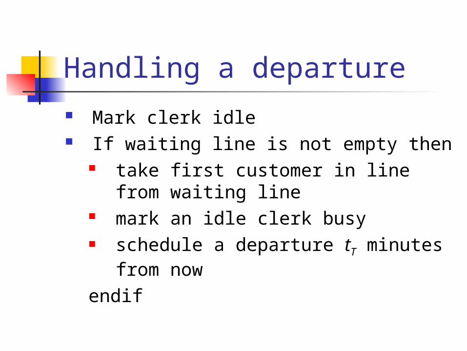
Handling a departure Mark clerk idle If waiting line is not empty then

take first customer in line from waiting line

mark an idle clerk busy schedule a departure tT minutes

from nowendif

Observations This simulation code will work for whatever

distribution of interarrival times and service times Not true for algebraic models

Nothing happens to the system between two consecutive events

Key issue is how to process these events at the time they are supposed to happen Will keep event notices in a event list

Event notices

Think of even notices as Post-it© notes describing activities to perform at specific times

Keep them in order!

Arrival0h 15m

Departure0h 40m

Arrival0h 20m

Departure0h 50m

Arrival1h 10m

Sorting event notices

Arrival0h 15m

Departure0h 40m

Arrival0h 20m

Departure0h 50m

Arrival1h 10m

The event list (I) Priority queue containing event notices Each event notice contains

The event type The time at which it will occur Other parameters depending on

the nature of the simulation Event list is kept sorted in

ascending event times

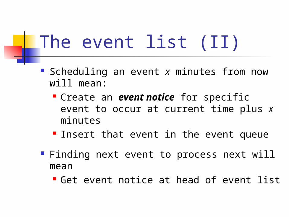
The event list (II) Scheduling an event x minutes from now

will mean: Create an event notice for specific

event to occur at current time plus x minutes

Insert that event in the event queue

Finding next event to process next will mean Get event notice at head of event list

General organization Initialize the system For ever do

get next event notice from event list execute appropriate event handling

routine(which will schedule new events)

od

That’s easy!

How to end the simulation? Several solutions:

Stop when a specific number of arrivals, failures, … have occurred/processed

Add to event list a “Finish” event with the appropriate time parameter.

Which tools can we use?

The modeling process We should build the model first before

thinking of any specific implementation Key issue is which aspects of system we

want to investigate Performance of a disk array? Reliability of same disk array? Capacity planning?

Entities Should first identify relevant entities in

the system Customers and clerks in post office

model Disks in disk array Waiting line in post office

Should distinguish between Permanent entities Temporary entities can be created

and disappear

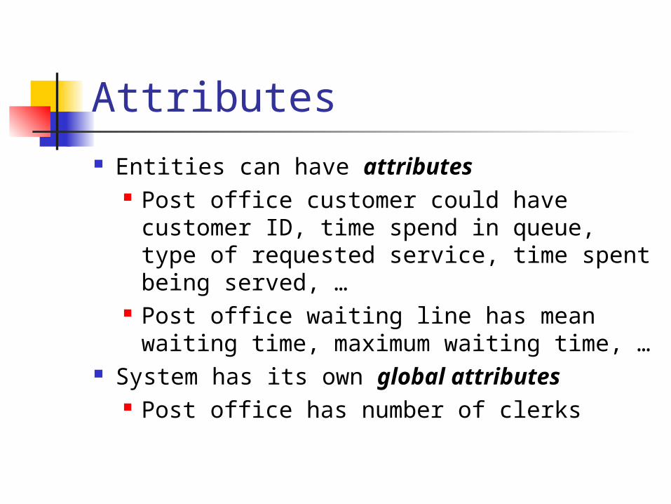
Attributes Entities can have attributes

Post office customer could have customer ID, time spend in queue, type of requested service, time spent being served, …

Post office waiting line has mean waiting time, maximum waiting time, …

System has its own global attributes Post office has number of clerks

More on entities and attributes Deciding which attributes should be

tracked will affect the complexity of the simulation program Especially attributes of temporary

entities Process-oriented simulation languages

include language-specific entities that simplify coding Facilities, storages

Programming tools We can use

A general-purpose language Because we have it

An event-oriented simulation language

Easiest to write An process-oriented simulation

language Easiest to use

A domain-specific simulation package Tailored to one area of application

General-purpose languages Nothing to buy, nothing to learn But

Must manage event list Must manage temporary entities that

have attributes Must collect all statistics

A simplistic example Program written in Perl Simulates a pair of mirrored disks

Assume exponential failures and repairs

Events are disk failures and disk repairs

Entities are two disks Disk attribute is disk status Global attributes include

Disk failure and repair rates Number of data losses

Why Perl Offers more powerful constructs than C Syntax based on that of Cshell Reasonably efficient for small simulations Watch for

my keyword marking first use of a new variable

Odd way to pass parameters through @_ array

Use of hashes for event list

What is a “hash”? A kind of array with arbitrary indices We will use them for storing the event list

%evtype will store the type of event:failure, repair, termination

%evdisk will store the affected disk To schedule a failure of disk 0 at time then

$evtype{$then} = “F”;$evdisk{$then} = 0;

Declarations

# declarationsmy $clock = 0.0; # timemy %evtype = (); # hashmy %evdisk = (); # hash

my $duration = 1000000000; #10^9my @status = (1, 1); # arraymy $losscount = 0;my $type = "E"; # error code

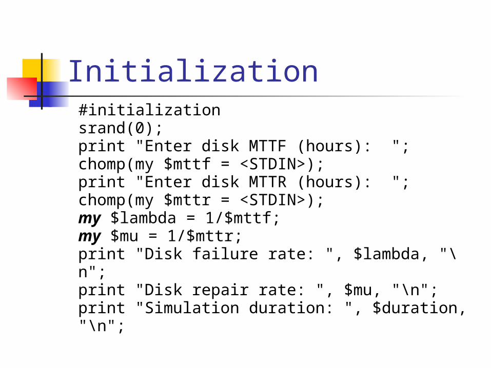
Initialization#initializationsrand(0);print "Enter disk MTTF (hours): ";chomp(my $mttf = <STDIN>);print "Enter disk MTTR (hours): ";chomp(my $mttr = <STDIN>);my $lambda = 1/$mttf;my $mu = 1/$mttr;print "Disk failure rate: ", $lambda, "\n";print "Disk repair rate: ", $mu, "\n";print "Simulation duration: ", $duration, "\n";

Set terminating event and schedule initial failures

# set terminating event&schedule($duration, "X", 2);# “X” stands for exit

# schedule initial failures&schedule(&exponential($lambda), "F", 0);&schedule(&exponential($lambda), "F", 1);# "F" stands for failure

Main loop

do { ($clock, $type, my $disk) = &nextevent; if ($type eq "F") { # disk failure &failure($disk); } elsif ($type eq "R") { # disk repair &repair($disk) } # if-else} while ($type ne "X"); # do-while

Processing a failure

sub failure { (my $failed) = @_; # extract disk ID $status[$failed] = 0; print "Disk $failed failed at time $clock.\n"; # check for data loss if ($status[1 - $failed] == 0) { $losscount++; print "Data loss at time $clock.\n"; } # if

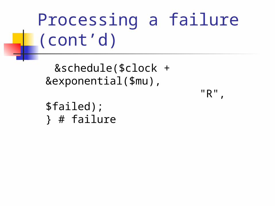
Processing a failure (cont’d)

&schedule($clock + &exponential($mu), "R", $failed);} # failure

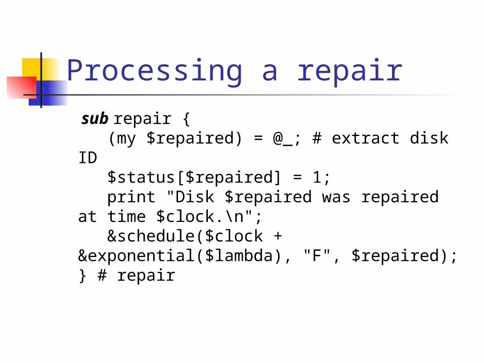
Processing a repair

sub repair { (my $repaired) = @_; # extract disk ID $status[$repaired] = 1; print "Disk $repaired was repaired at time $clock.\n"; &schedule($clock + &exponential($lambda), "F", $repaired);} # repair

Closing

#closingprint "SIMULATION RESULTS:\n";print "Number of data losses is $losscount.\n";my $mttdl = $duration/$losscount;print “Rough estimate of MTTF is $mttdl.\n";# end of simulation

Schedule an event

sub schedule() {# extract three parameters

(my $thistime, my $thistype, my $thisdisk) = @_; $evtype{$thistime} = $thistype; $evdisk{$thistime} = $thisdisk;} # schedule

Get next event

sub nextevent { my @skeys = sort{$a <=> $b} (keys %evtype); my $thattime = shift(@skeys); my $thattype = $evtype{$thattime}; my $thatdisk = $evdisk{$thattime}; delete($evtype{$thattime}); delete($evdisk{$thattime}); ($thattime, $thattype, $thatdisk);} nextevent

Generating exponentially distributed random numbers

#!/usr/bin/perl -w# mere mirrored data

use strict;

sub exponential {(my $rate) = @_;- log(rand(1))/$rate;} # exponential

More details later

More general comments Always use a floating-point variable for

the simulated time It minimizes the risk of having two

events happening at the same time All global attributes are represented by

global variables Possible customer attributes such as

arrival times would be represented by dynamic data structures

Event-orientedsimulation languages Extensions of a general-purpose

language that offer tools to Manage the event list Insert entities in a queue and

removing them Collect statistics

Programmer’s main task is to write theevent routines

Can write your own extensions

Process-orientedsimulation languages Allow programmer to describe system’s

behavior in terms of actions taken by active entities (processes)

Easiest to use Can be

Extensions of a general-purpose language (CSIM)

Full-fledged languages (Simscript)

Post office revisited Customer will

Enter the system Request service from one of the

clerks and wait until a clerk is available

Mark that clerk busy Hold the clerk busy for service_time Release the clerk Leave the system

Post office revisited (cont’d) Main program will Read system parameters For i = 1 to max_customers do

Hold for interarrival_time Create a customer process

Wait for completion of last customer Print statistics

Facilities A facility is an entity that

Can only be occupied by one process Includes an associated queue

A process may Request usage of a facility:

process will wait in queue if facility is busy

Release the facility:process at the head of the queue will get the facility

Storages A storage is an entity that

Has a finite capacity Includes an associated queue

A process may Request x units of storage:

process will wait in queue if facility is busy

Release the facility:process at the head of the queue will get its request reconsidered

Usage Facilities and storage are often used to

represent servers A set of n servers can be represented

By an array of facilities of size n (if language allows arrays of facilities)

By a storage of capacity n Each customer then requires one unit

of storage Think of facilities as some kind of

semaphores

CSIM Simulation language developed by

Mesquite Software in Austin, TX C/C++ based Most likely to encounter

CSIM Basic Example (I)

Single server and its waiting line Customers interarrival times are exponentially

distributed with mean equal to one time unit Service times are also exponentially

distributed with mean equal to 0.5 time unit

Waiting line Server

CSIM Basic Example (II)

System entities include The system itself

Will be represented by the main process

The customers Will be represented by processes

The server Will be represented by a facility

CSIM Basic Example (III)

The system process will Generate the customer processes at

the specified time intervals The customer processes will

Wait until the server is free Hold it for the specified time interval

CSIM Basic Example (IV)

#include <cpp.h> // CSIM C++ header filefacility *f; // the service center extern "C" void sim()  {   // sim process

create("sim"); // make this a processf = new facility("f"); // create facility

while (simtime() < 5000.0) { hold(exponential(1.0)); // delay cust(); // create process

} // whilereport(); // output results

} // sim  

Explanations CSIM program structure is constrained

by its host language Must do a create() at the beginning of

each function describing a process The hold(…) function simulates a delay

by suspending the sim process for the specified amount of simulated time There is no busy wait

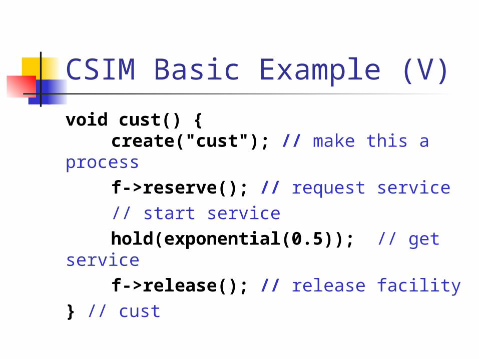
CSIM Basic Example (V)

void cust() { create("cust"); // make this a process

     f->reserve(); // request service// start servicehold(exponential(0.5)); // get servicef->release(); // release facility

} // cust 

Other features CSIM has great measurement tools to

evaluate quantities like Number of customers waiting for

service Customer waiting times Customer service times …

Simscript Simulation language developed by

CACI in Torrey Pines, CA Full fledged language with a long

history Now Simscript II.5

Most powerful

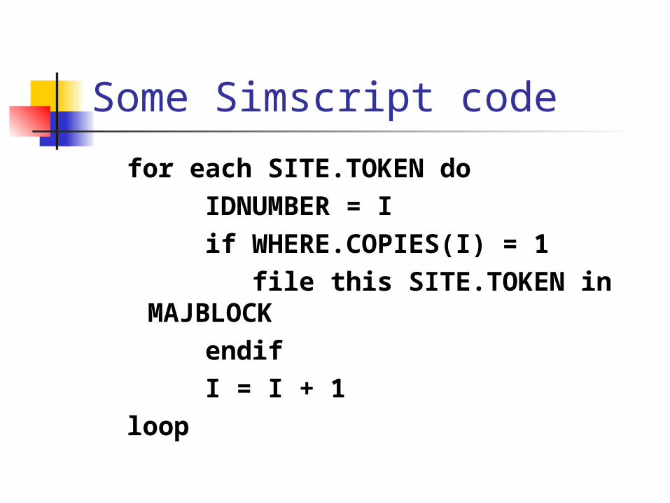
Some Simscript code

for each SITE.TOKEN do

IDNUMBER = I

if WHERE.COPIES(I) = 1

file this SITE.TOKEN in MAJBLOCK

endif

I = I + 1

loop

Observations Main advantage of Simscript is its clean

structure: Language is specifically tailored to

discrete simulation applications Sole drawback is need to learn a new

language

Domain-specific application packages Network simulator 2 (Ns-2)

Discrete event simulator targeted at networking research

Offers “substantial support” for simulation of TCP, routing, and multicast protocols over both wired and wireless networks

Uses an object-oriented version of Tcl (OTcl) for user-specified scripts

Will have to learn/love Tcl syntax

Domain-specific application packages (cont’d) General Peer-to-Peer Simulator (GPS)

Allows accurate modeling and efficient simulation of P2P protocols and applications.

Models communication at the message level

Still takes into account the underlying network and protocol properties ( TCP)

How to generate random numbers?

The problem Must often generate random variables

that are distributed according to a specific distribution Interarrival times are often distributed

according to an exponential distribution Service times could be uniformly

distributed between a minimum and a maximum service time

Gaussian distributions often appear in network simulation

The starting point Nearly all computers have a library function

generating pseudo-random numbers Random integers between 0 and 2n – 1 Random floating-point numbers uniformly

distributed between 0 and 1 You should keep in mind that

The numbers only appear to be random Some random number generators are

better/worse than the others

Classical random number generators Linear congruential generators

Use the recurrence

Xn+1 = (a Xn + b) % m

Numerical Recipes in C suggests using:

a = 1664525, c = 1013904223, m = 232

Better random number generators exist

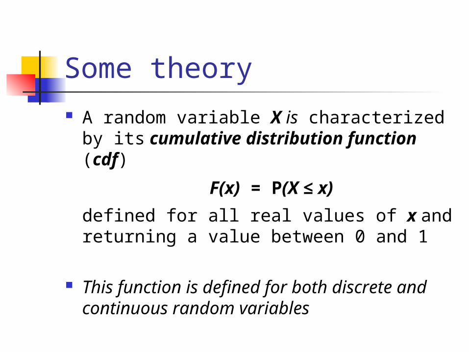
Some theory A random variable X is characterized by

its cumulative distribution function (cdf)

F(x) = P(X ≤ x)

defined for all real values of x and returning a value between 0 and 1

This function is defined for both discrete and continuous random variables

An example:cdf of normal distribution

More theory Assume that we have a random number

generator producing random values that are uniformly distributed on [0, 1]

random() Then F-1 (random()) will generate

random numbers distributed according to the cdf F(x)

A justification Assume that U is a random variable that is

uniformly distributed between 0 and 1 Since F () is a monotonic function

P(F-1(U ) ≤ x ) = P( F (F-1(U )) ≤ F (x )) If F () is invertible

P(F (F-1(U ) ≤ F (x )) = P( U ≤ F (x )) Since U is uniformly distributed over [0, 1)

P( U ≤ F (x )) = F (x )

Application to uniform distribution Uniform distribution states that random

variable x has equal probabilities to take any value in some interval [a, b]

Its probability density function isf(x) = 1/(b - a) for a ≤ x < b and 0 elsewhere

Its cdf isF(x) = (x – a)/(b - a) for a ≤ x < b

Cdf of U(a, b)

1

0

a b

Input: value in range

Output:value of cdf

F(x) = (x – a)/(b - a) for a ≤ x < b

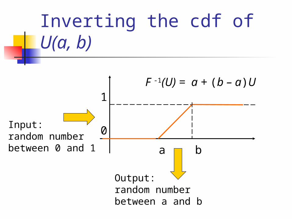
Inverting the cdf of U(a, b)

1

0

a b

Output:random numberbetween a and b

Input:random numberbetween 0 and 1

F -1(U) = a + (b – a)U

Application to uniform distribution (continued) Its cdf is

F(x) = (x – a)/(b – a) for a ≤ x < b 0 for x < a

1 for x b The inverse of the cdf is

F -1(U) = a + (b – a)U

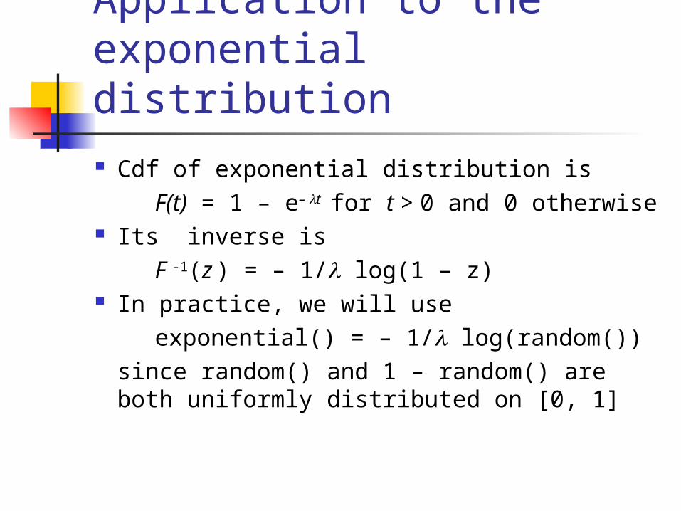
Application to the exponential distribution Cdf of exponential distribution is

F(t) = 1 – e– t for t > 0 and 0 otherwise Its inverse is

F -1(z ) = – 1/ log(1 – z) In practice, we will use

exponential() = – 1/ log(random())since random() and 1 – random() are both uniformly distributed on [0, 1]

Application to the normal distribution (I) Box-Muller algorithm

If we have two numbers a and b uniformly distributed on (0, 1], then c and d such that

c = (– 2 ln a) cos (2b)d = (– 2 ln a) sin (2b)

are normally distributed

Application to the normal distribution (II) Ziggurat method:

Faster See

http://www.cse.cuhk.edu.hk/~phwl/mt/public/archives/papers/grng_acmcs07.pdf

Application to discrete distributions Consider a RV X having only two

possible values, a and b Assume

P(X = a) = pP(X = b) = 1 – p

Cdf of RV is a staircase function First step for x = a Second step for x = b

Cdf of RV

1

0

a b

Input: value in range

Output:value of cdf

p

1 – p

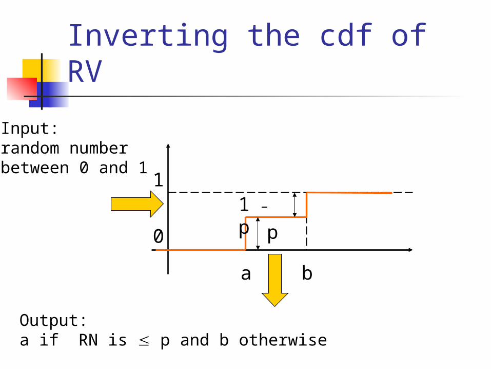
Inverting the cdf of RV

1

0 p

1 – p

Input:random numberbetween 0 and 1

Output:a if RN is p and b otherwise

a b

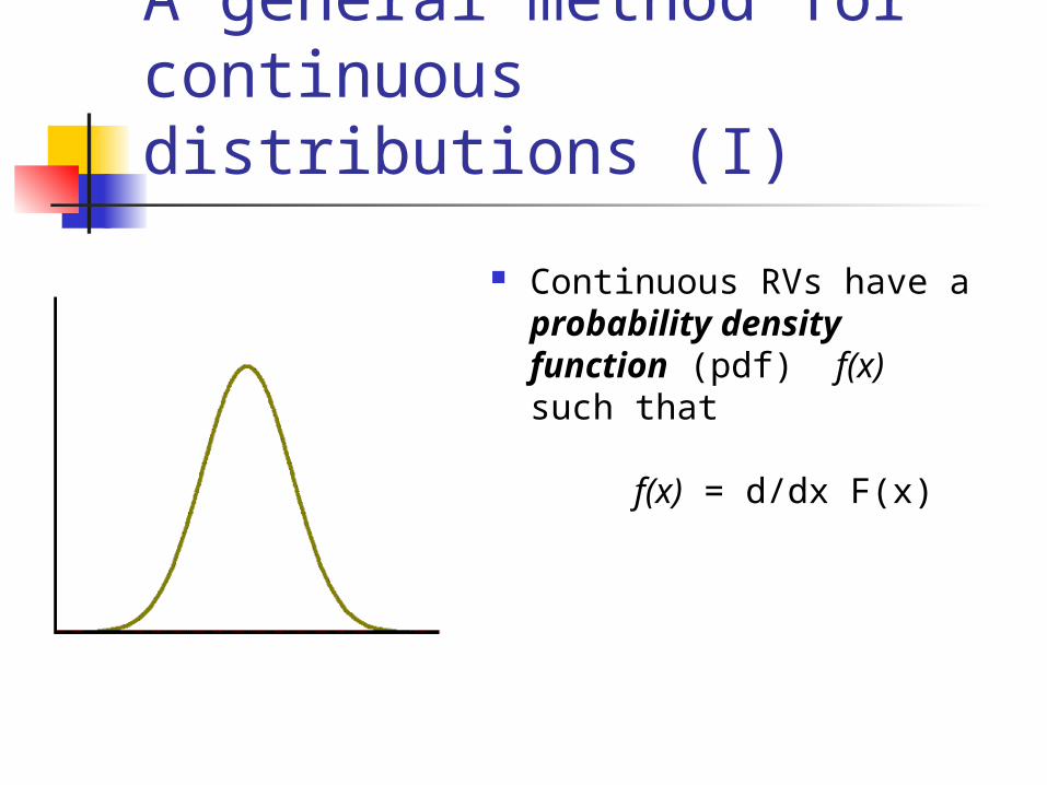
A general method for continuous distributions (I)

Continuous RVs have a probability density function (pdf) f(x) such that

f(x) = d/dx F(x)

A general method for continuous distributions (II)

Build a rectangular box around the pdf of the distribution

Generate two RVs X = U(a, b) Y = U(0,c)

Accept X if point (X,Y) falls below the curve

a b

c

YES

NONO NONO

Last but not least:What about “reseeding” Pseudo-random number generators

generate deterministic sequences of pseudo-random numbers Two sequences starting with the

same seed value will be identical Great for debugging Must reseed each time with a

different value when making multiple runs of the same program

How to collect measurements?

Overview We collect measurements by adding

counters that keep track of Number of entities serviced Service times …

Facilities, Storages and Queues These three resources normally contain

other entities Assume two counters for one of these

entities SumOfTimesIn: incremented by the

current value of the simulation clock when an entity enters the resource

SumOfTimesOut: incremented by the current value of the simulation clock when an entity leaves the resource

Facilities, Storages and Queues (continued) Then

SumOfTimesIn – SumOfTimesOut represents the total time TotalTimeIn spend by all entities in the resource

If we divide TotalTimeIn by the number of entities that went though the resource, we get the average time spent by each entity inside the resource

Facilities, Storages and Queues (continued)

If we divide TotalTimeIn by the current value of the simulation clock,we get a average number of entities in the resource, that is, its average occupancy

An example Consider the waiting line of our post office

Assume that 10 customers visited the post office and spent a total of 30 minutes in the waiting line over a one hour period

The average customer waiting time is 3 minutes

The average queue length is 0.5 customers How do we get that?

Explanation If 10 people spent a total of 30 minutes

waiting for service over a one-hour period, A total of 30 customer-minutes were

spent in the queue The average queue length is 30/60 =

0.5

Collecting other statistics Maximum and minimum queue lengths

are not hard to compute Statistics about temporary entities are

harder to collect Must associate attributes with each

instance of a particular temporary entityA great motivation for not using a general purpose programming language

Statistical Analysis Most of statistical analysis techniques

do not apply to the data collected during a simulation study because they arenot mutually independentPeople arriving at the post office when the waiting line is longer than usual will wait more than the average wait time

Must use batch means method or regeneration method

FURTHER LEARNING The web is a good starting point