an introduction to simulation optimization · an introduction to simulation optimization 1. 1. ......
TRANSCRIPT
Nanjing Jian
Shane G. Henderson
Introductory Tutorials
Winter Simulation Conference
December 7, 2015
Thanks: NSF CMMI1200315
An Introduction to
Simulation Optimization
1

1. Introduction
2. Common Issues and Remedies
3. Tools
4. Case Study: Bike Sharing
Contents
2

Choosing the decision variables
to optimize some (expected)
performance measure.
What is Simulation Optimization?
Other names: “Simulation-based Optimization” or
“Optimization via Simulation”.
Simulation
Simulation Model
+
Having uncertainty in the
objective and/or constraints.
Optimization
Optimization Model
+
3
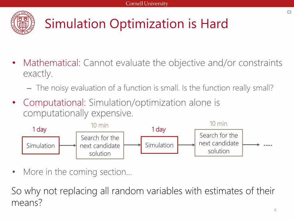
Simulation Optimization is Hard
• Mathematical: Cannot evaluate the objective and/or constraints exactly.
– The noisy evaluation of a function is small. Is the function really small?
• Computational: Simulation/optimization alone is computationally expensive.
• More in the coming section…
So why not replacing all random variables with estimates of their
means?
Simulation
Search for the
next candidate
solution
Simulation
Search for the
next candidate
solution
…..
1 day 1 day10 min 10 min
4
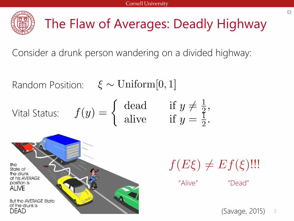
The Flaw of Averages: Deadly Highway
(Savage, 2015)
Random Position:
Vital Status:
“Alive” “Dead”
Consider a drunk person wandering on a divided highway:
5
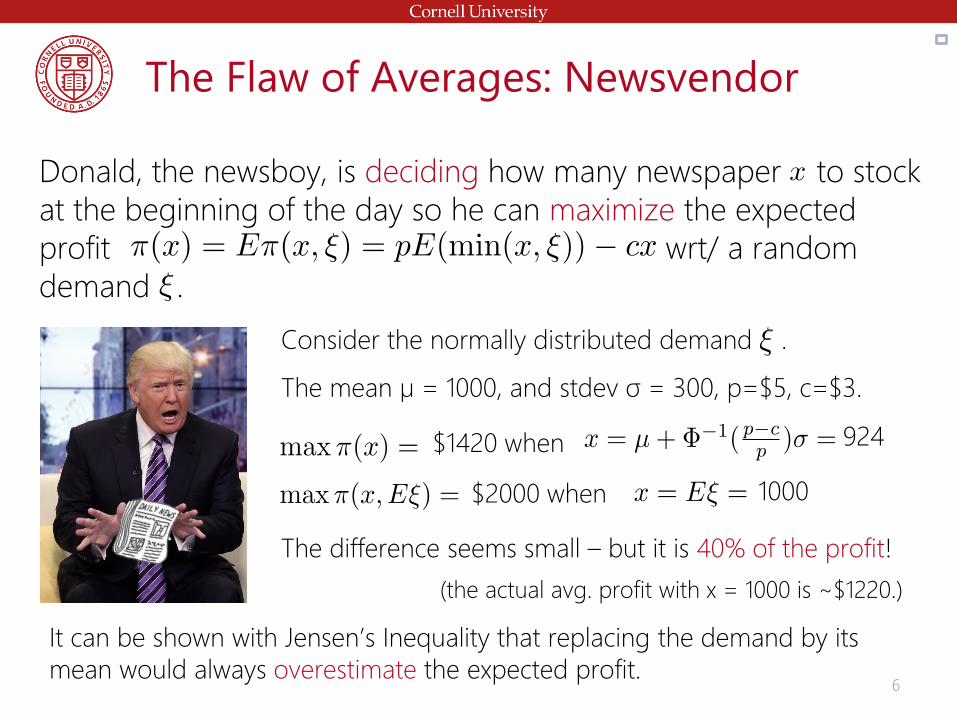
Consider the normally distributed demand .
The mean µ = 1000, and stdev σ = 300, p=$5, c=$3.
It can be shown with Jensen’s Inequality that replacing the demand by its
mean would always overestimate the expected profit.
The difference seems small – but it is 40% of the profit!
(the actual avg. profit with x = 1000 is ~$1220.)
Donald, the newsboy, is deciding how many newspaper to stock
at the beginning of the day so he can maximize the expected
profit wrt/ a random
demand .
The Flaw of Averages: Newsvendor
6
$2000 when
$1420 when 924
1000
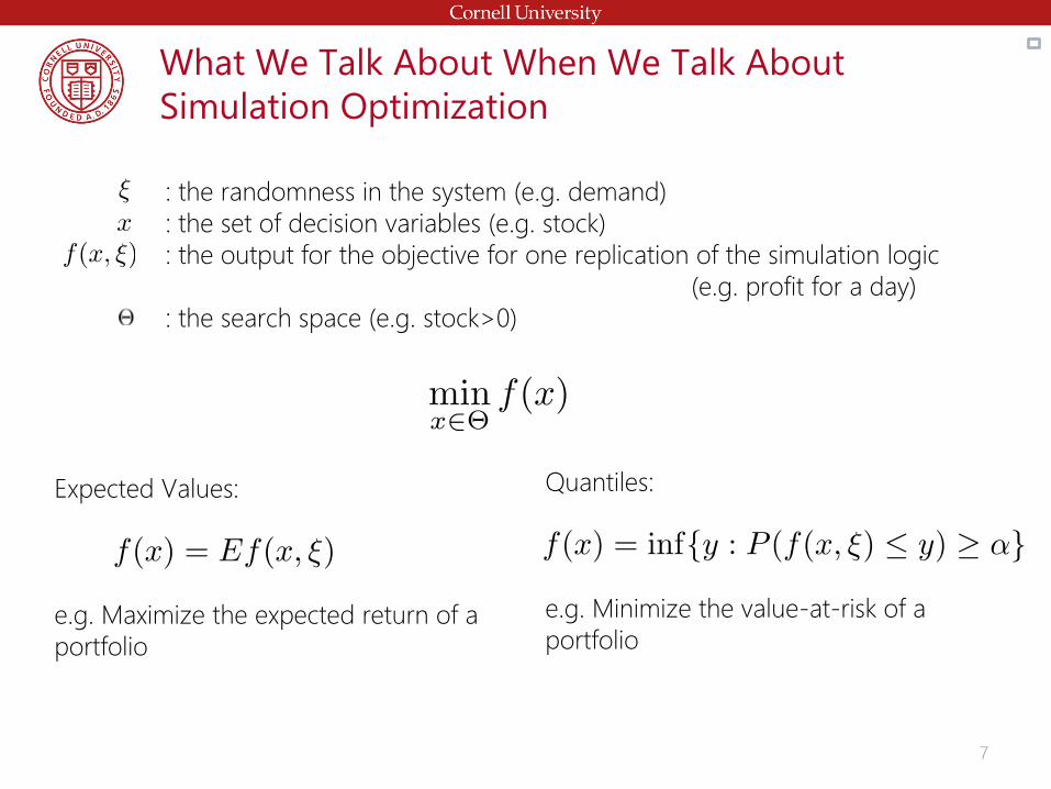
What We Talk About When We Talk About
Simulation Optimization
Quantiles:
e.g. Minimize the value-at-risk of a
portfolio
Expected Values:
e.g. Maximize the expected return of a
portfolio
: the randomness in the system (e.g. demand)
: the set of decision variables (e.g. stock)
: the output for the objective for one replication of the simulation logic
(e.g. profit for a day)
: the search space (e.g. stock>0)
7

Problem
Newsvendor Demand Starting inventory (-) Daily profit
Financial Optimization Stock
Price
Portfolio (-) Return
Supply Chain Inventory (s-S) Demand Base stock level
(Order-up-to level)
Inventory holding
cost
Queuing System, e.g. Call
centers
Arrivals Number of Servers Waiting time
Healthcare, e.g. Ambulance Call
Arrivals
Base locations Response time
Applications of Simulation Optimization
8
Scope and Other References
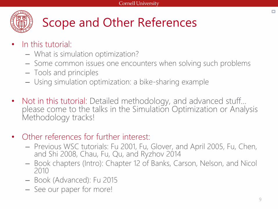
• In this tutorial:– What is simulation optimization?
– Some common issues one encounters when solving such problems
– Tools and principles
– Using simulation optimization: a bike-sharing example
• Not in this tutorial: Detailed methodology, and advanced stuff… please come to the talks in the Simulation Optimization or Analysis Methodology tracks!
• Other references for further interest:– Previous WSC tutorials: Fu 2001, Fu, Glover, and April 2005, Fu, Chen,
and Shi 2008, Chau, Fu, Qu, and Ryzhov 2014
– Book chapters (Intro): Chapter 12 of Banks, Carson, Nelson, and Nicol 2010
– Book (Advanced): Fu 2015
– See our paper for more!
9

1. Introduction
2. Common Issues and Remedies
3. Tools
4. Case Study: Bike Sharing
Contents
10

Local vs. Global Solutions
Minimum???
• Similar to finding the lowest point in the US, but:
- in heavy fog: only local information available
- with a broken altimeter: can only measure altitude with noise
- and a teleporter machine: can sample anywhere
How to differentiate The Grand Canyon from Death Valley?
• Searching on a function:
– Global optimum: the true minimum/maximum on the entire domain.
– Local optimum: the point where no nearby improvement can be found.
11

Local vs. Global Solutions
• Unless the function is convex, the best an algorithm can
promise is to locate a local minimum.
• Solution: Can use random restart:
– Not-too-rolling landscape: may be effective
– Very-rolling landscape: will visit the global minimum eventually… after
lots of restarts!
Start 1
End 1
Start 2
End 2
Start 3
Start 4
End 4
(3)
12
Many Decision Variables =
Huge Search Space
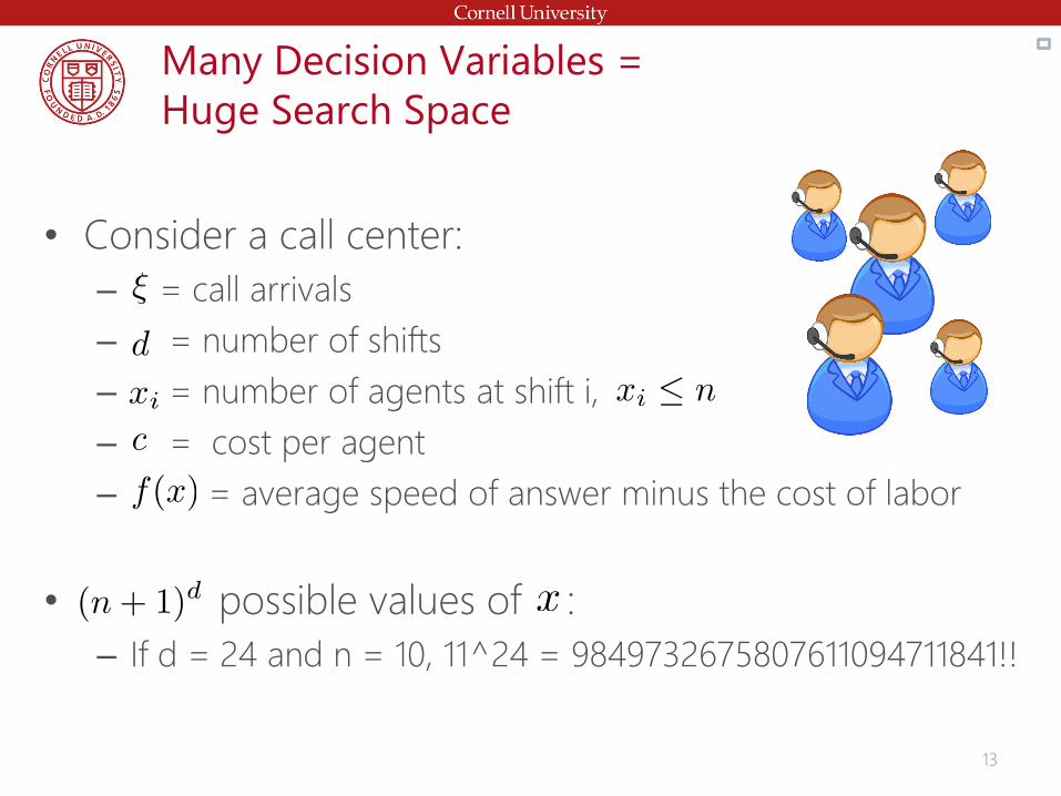
• Consider a call center:
– = call arrivals
– = number of shifts
– = number of agents at shift i,
– = cost per agent
– = average speed of answer minus the cost of labor
• possible values of :
– If d = 24 and n = 10, 11^24 = 9849732675807611094711841!!
13
Huge Search Space: What can we do?
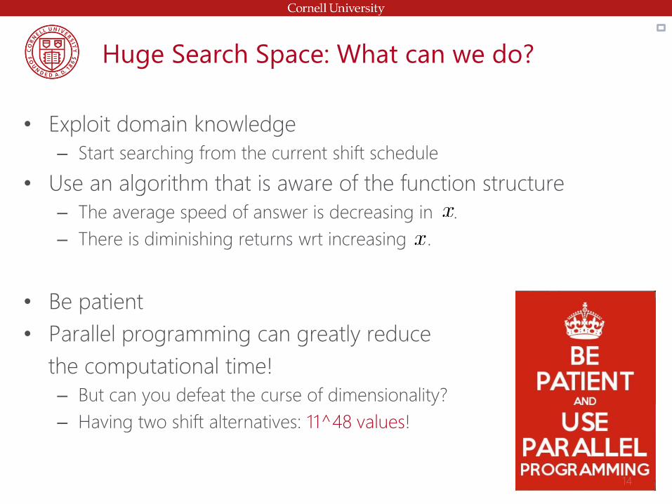
• Exploit domain knowledge
– Start searching from the current shift schedule
• Use an algorithm that is aware of the function structure
– The average speed of answer is decreasing in .
– There is diminishing returns wrt increasing .
• Be patient
• Parallel programming can greatly reduce
the computational time!
– But can you defeat the curse of dimensionality?
– Having two shift alternatives: 11^48 values!
14

Continuous vs. Discrete Decision Variables
• Continuous decision variables:
– There are efficient local search algorithms that can exploit
continuity and differentiability.
– “Close” points are expected to have “close” function values.
• Discrete decision variables:
– “Continuity” doesn’t come naturally.
15
Optimizing in the Presence of Noise
• Suppose in replication i, we obtain output . Let the
objective be denoted as .
• How far is from ?
• If , does it imply ?
• Solution: We can increase the runlength at and to be
more sure.
– But how about other values?
16

• When the difference in the simulation noise is bigger than the difference in the function values:
• Solutions:
– Carefully choose the runlength to ensure statistically significant differences
– Use Common Random Numbers
x2x1
Simulation Noise can Swamp the Signal
17
True f
(unknown)
Smaller??CI for the sample means
Estimation errors of the sample average
f(x1)
f(x2)
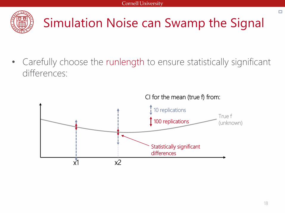
Simulation Noise can Swamp the Signal
• Carefully choose the runlength to ensure statistically significant
differences:
18
x1 x2
True f
(unknown)100 replications
10 replications
CI for the mean (true f) from:
Statistically significant
differences

Common Random Numbers (CRN)
• Idea: Use the same set of to evaluate and .
• E.g. Consider the newsvendor problem: – Comparing starting stocks and .
– CRN means comparing the two with exact the same demands.
• To use: Many software has random number stream implemented. Use the same stream to simulate the systems being compared.
19
x1 x2
True f
(unknown)

Failing to Recognize an Optimal Solution
Even if we visited every point in the solution space, how do we
know which one is optimal, given we can only obtain noisy
evaluations of the objective?
• Again, carefully choose runlength.
• Use ranking & selection to “clean up” the solutions! † (later)
† : Hong, Nelson, and Xu 201520
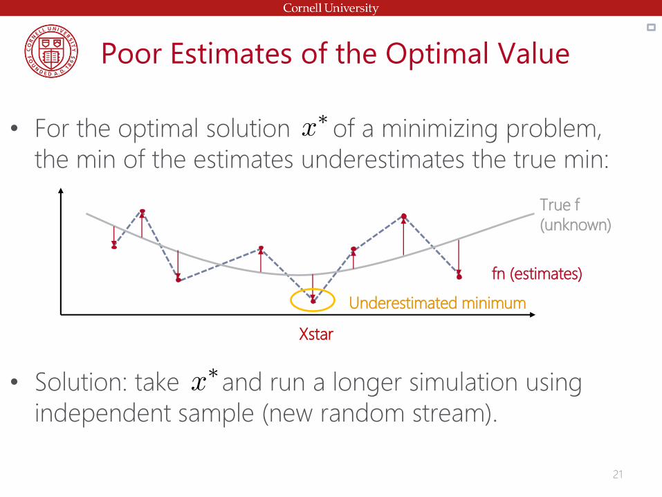
Poor Estimates of the Optimal Value
• For the optimal solution of a minimizing problem,
the min of the estimates underestimates the true min:
• Solution: take and run a longer simulation using
independent sample (new random stream).
Xstar
True f
(unknown)
fn (estimates)
Underestimated minimum
21
When to stop?
• Since objective is noisy, it is hard to differentiate noise from the
actual progress. Usually most algorithms are stopped when a
computational budget is reached.
• “Smarter” ways to stop:
– Start the optimization algorithm with a small number of
replications.
– Then sequentially increase the sample size to “refine” the
solution until “steady”.
22
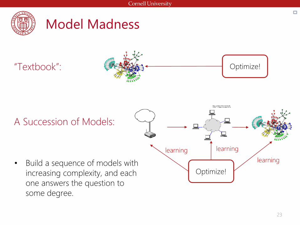
Model Madness
“Textbook”:
A Succession of Models:
Optimize!
• Build a sequence of models with
increasing complexity, and each
one answers the question to
some degree.
Optimize!
learning learning
learning
23
Summary
We talked about issues arising from:
• Nonlinear Optimization:– Local vs. Global solutions
– Huge search space
– Discrete vs. Continuous variables
• Simulation Noise:– Optimizing in the presence of noise
– Simulation noise can swamp the signal
– Failing to recognize an optimal solution
– Getting poor estimates of the objective of the estimated optimal solution
– When to stop
• Modeling:– Model Madness
24
1. Introduction
2. Common Issues and Remedies
3. Tools
4. Case Study: Bike Sharing
Contents
25

Sample Average Approximation
• Idea: Use sample average ( ) to estimate
the expectation ( ).
– If the inputs are fixed, optimizing is a deterministic
program.
• To use: Assign a stream of random numbers to rep i.
• Pros: Very flexible, works on constrained problems, and reliable
when n is large
• Cons: User needs to choose the deterministic optimization
algorithm.
• Example: Call center:– Wish to optimize the expected customer waiting time
– Use the average customer waiting time over 1000 simulated days as an estimate
– Optimize this average with different staffing schedules over the same 1000 days
(using CRN)More: Kim, Pasupathy, and Henderson 2015. 26
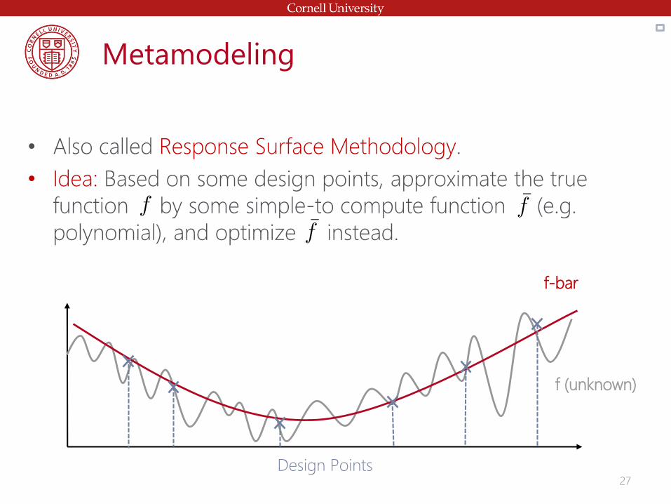
Metamodeling
• Also called Response Surface Methodology.
• Idea: Based on some design points, approximate the true
function by some simple-to compute function (e.g.
polynomial), and optimize instead.
f (unknown)
f-bar
27
Design Points

• Global metamodel: Used when the search space is small.
• Local metamodel: Used to move to the next candidate solution.
• Pros: The metamodel is structured and thus easy to optimize.
• Cons: Relies on the experiment design, needs smoothness to
work well
Metamodeling
More: Barton 2009, Kleijnen 2015.28
f (unknown)
Design Points
f-bar
x0 x1
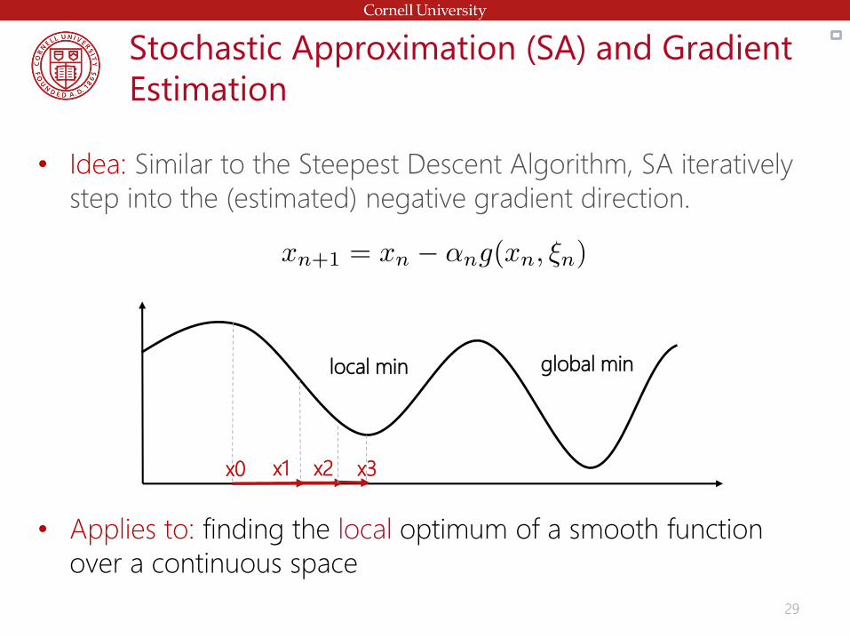
Stochastic Approximation (SA) and Gradient
Estimation
• Idea: Similar to the Steepest Descent Algorithm, SA iteratively
step into the (estimated) negative gradient direction.
local min global min
x0 x1 x2 x3
29
• Applies to: finding the local optimum of a smooth function
over a continuous space
Stochastic Approximation (SA) and Gradient
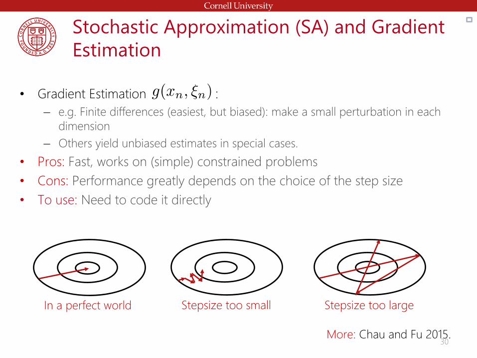
Estimation
• Gradient Estimation :
– e.g. Finite differences (easiest, but biased): make a small perturbation in each
dimension
– Others yield unbiased estimates in special cases.
• Pros: Fast, works on (simple) constrained problems
• Cons: Performance greatly depends on the choice of the step size
• To use: Need to code it directly
More: Chau and Fu 2015.
In a perfect world Stepsize too small Stepsize too large
30
Ranking and Selection
• Idea: Exhaustively test all solutions and rank them. The goal is to return the system with the lowest mean.
• A common frequentist procedure:
1. Start by obtaining a small sample (say, 10) on each system.
2. Use the initial sample to decide how much to further simulate each system.
• The procedures differs by the allocation of samples and the statistical guarantee provided.
• The total sample sizes can be different for each system!
– The choice of sample sizes can be quite complicated.
– Usually it is larger for the system with higher variance and/or closer to the optimum.
31
• Algorithms providing PCS/PGS guarantees are usually very conservative.
• Other methods that are more efficient but without guarantee:
- “Optimal Computing Budget Allocation” for maximizing PCS/PGS †.
- “Expected Value of Perfect Information” for the most “economic”
choice ‡.
Ranking and Selection: Statistical Guarantee
User input:
• Probability of correct selection (PCS):
– Guarantees (say, w.p. 95%) to choose the best
system only if it is better than the second best
by at least
– is called the “indifference zone” parameter.
• Probability of good selection (PGS):
– Guarantees (say, w.p. 95%) the selected system
is worse than the best system by at most
†:‡: see Chen, Chick, and Lee 2015; More: Kim and Nelson 2006. 32
Guarantees if
Guarantees
Ranking and Selection
• Applies to: A finite and “small” (say, <500) search space, so
each solution can be estimated by at least a few simulation
runs.
• The recent development of using parallel computing in R&S can
handle larger search space (e.g. 10^6 systems) †.
• Example: Clean up step after an initial search
• To use: Implemented in some commercial software packages
33†: see Luo and Hong 2011, Luo et al. 2015, Ni et al. 2015
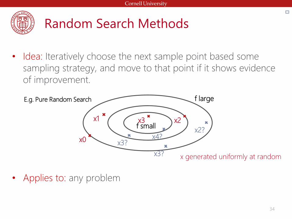
• Idea: Iteratively choose the next sample point based some
sampling strategy, and move to that point if it shows evidence
of improvement.
• Applies to: any problem
Random Search Methods
34
x0
x1
x2?
x2
x3?
x3?
x3
x4?
f large
f small
x generated uniformly at random
E.g. Pure Random Search
Random Search Methods
• The sampling strategy:
– deterministic or randomized
– depends on the information of all the previous points, only a few
previous points, or only the most recent point
– trades off exploration vs. exploitation
• Pros: Easy to implement, no requirement for problem structure
• Cons: Few or no statistical guarantee, not using any model
information
• Widely used in most commercial packages.
More: Andradottir 2015, Hong, Nelson, and Xu 2015, Fu, Glover,
and April 2005, Olafsson 2006. 35
1. Introduction
2. Common Issues and Remedies
3. Tools
4. Case Study: Bike Sharing
Contents
36

Problem Statement
• Citibike in NYC has approximately 330 stations and 6000 bikes.
• Users check out bikes at a station and return bikes to another
station.
• Unhappy bikers are those who don’t find a bike when they want
one, or don’t find a rack when they want one.
• In the event of a full rack, users go to a nearby bike station. A
bike may be abandoned after a few attempts.
†: www.siegelgale.com, www.voltaicsystems.com, socialmediaweek.org
†
37
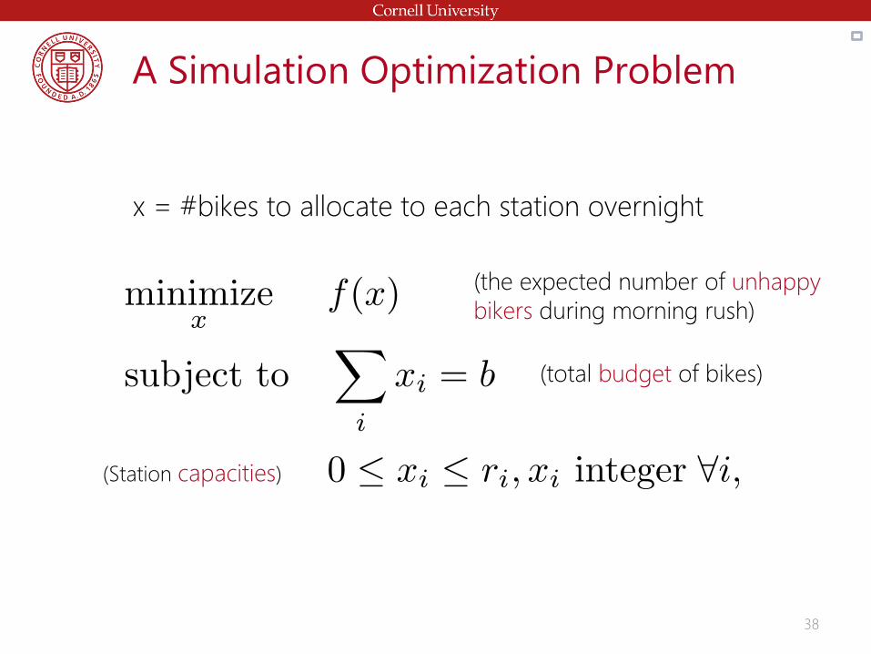
A Simulation Optimization Problem
(the expected number of unhappy
bikers during morning rush)
x = #bikes to allocate to each station overnight
(total budget of bikes)
(Station capacities)
38
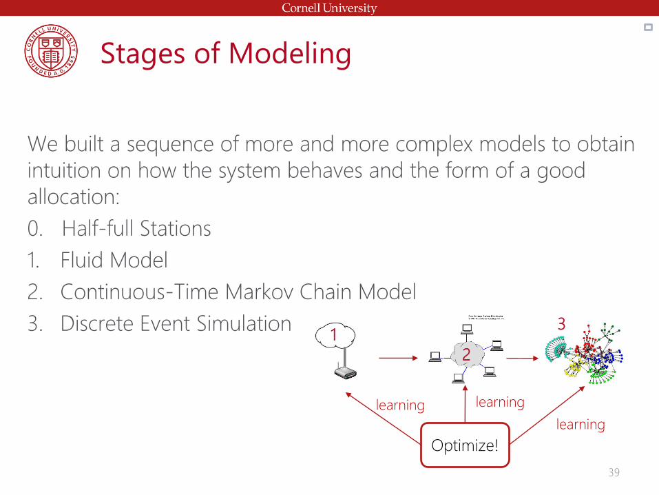
Stages of Modeling
We built a sequence of more and more complex models to obtain
intuition on how the system behaves and the form of a good
allocation:
0. Half-full Stations
1. Fluid Model
2. Continuous-Time Markov Chain Model
3. Discrete Event Simulation
Optimize!
learning learning
learning
1
2
3
39
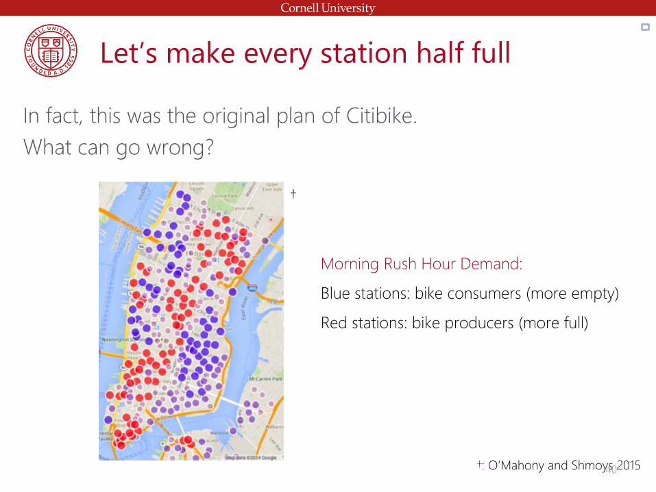
Let’s make every station half full
In fact, this was the original plan of Citibike.
What can go wrong?
Morning Rush Hour Demand:
Blue stations: bike consumers (more empty)
Red stations: bike producers (more full)
†: O’Mahony and Shmoys 2015
†
40
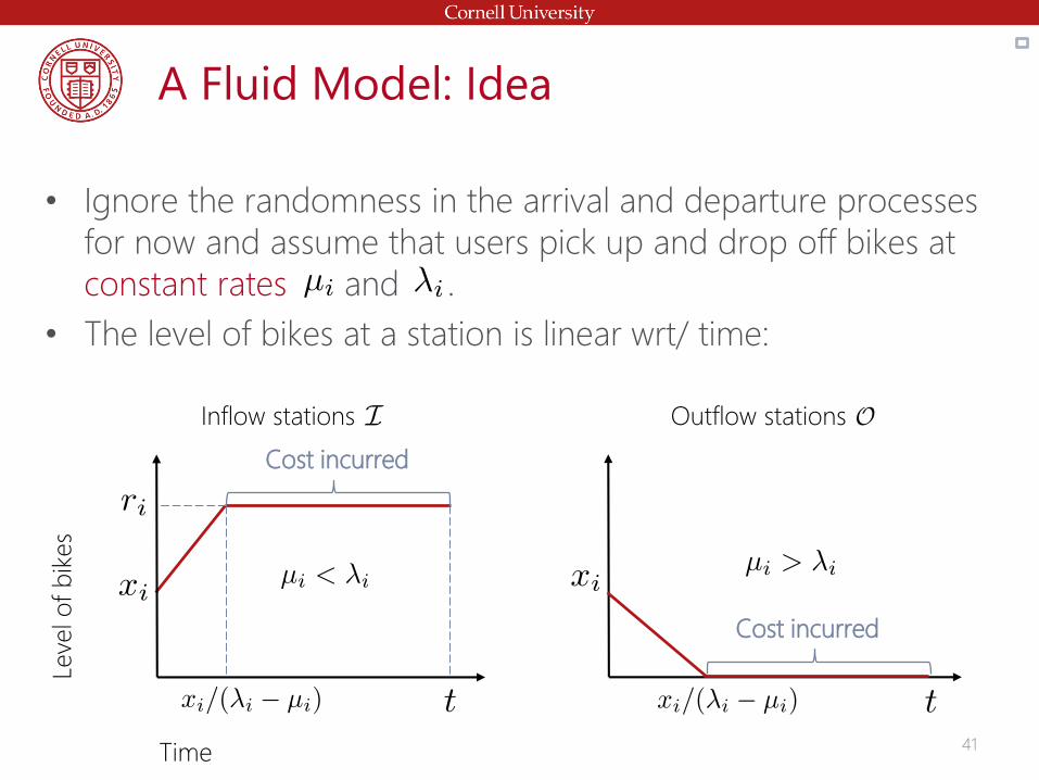
A Fluid Model: Idea
• Ignore the randomness in the arrival and departure processes
for now and assume that users pick up and drop off bikes at
constant rates and .
• The level of bikes at a station is linear wrt/ time:
Cost incurred
Leve
l o
f b
ikes
Time
Inflow stations
Cost incurred
Outflow stations
41
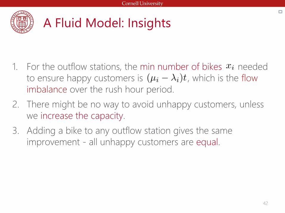
A Fluid Model: Insights
1. For the outflow stations, the min number of bikes needed
to ensure happy customers is , which is the flow
imbalance over the rush hour period.
2. There might be no way to avoid unhappy customers, unless
we increase the capacity.
3. Adding a bike to any outflow station gives the same
improvement - all unhappy customers are equal.
42
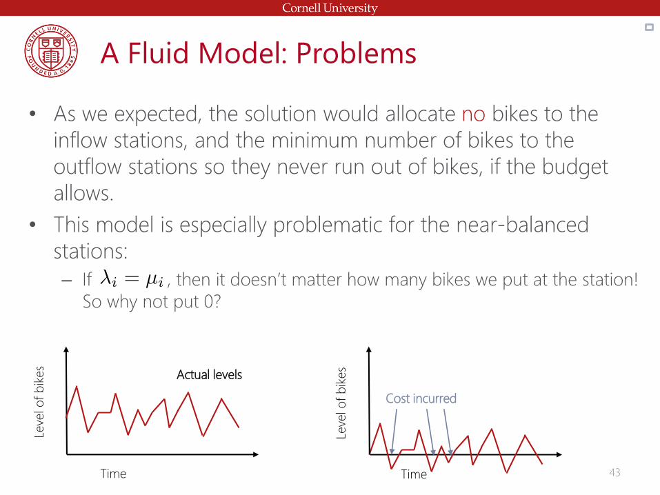
A Fluid Model: Problems
• As we expected, the solution would allocate no bikes to the
inflow stations, and the minimum number of bikes to the
outflow stations so they never run out of bikes, if the budget
allows.
• This model is especially problematic for the near-balanced
stations:
– If , then it doesn’t matter how many bikes we put at the station!
So why not put 0?
Leve
l o
f b
ikes
Time
Actual levels
Leve
l o
f b
ikes
Time
Cost incurred
43
A Continuous-Time Markov Chain Model
• Model the flows of customer arrivals at different stations as
independent time-homogeneous Poisson processes.
• Assume that the stations never run out of bikes, then each
station can be modeled as a queue independent of
all other stations.
• This is a strong assumption to make!
• This model captures the stochastic nature of bike flows.
– Once a station is full, it will not stay full for the rest of the period.
44
A Continuous-Time Markov Chain Model
• When , the solution .
• can be computed very efficiently without simulation.
• Also one can show f(x) is “convex”!
• This CTMC solution can be used as a starting solution for the
simulation optimization.
45
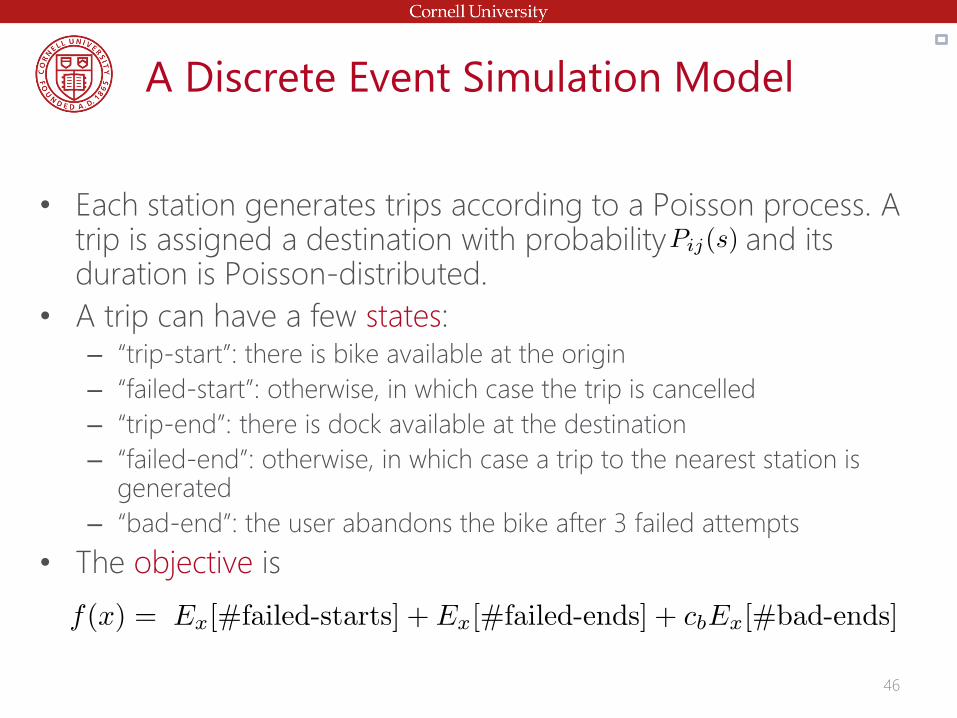
A Discrete Event Simulation Model
• Each station generates trips according to a Poisson process. A trip is assigned a destination with probability and its duration is Poisson-distributed.
• A trip can have a few states:– “trip-start”: there is bike available at the origin
– “failed-start”: otherwise, in which case the trip is cancelled
– “trip-end”: there is dock available at the destination
– “failed-end”: otherwise, in which case a trip to the nearest station is generated
– “bad-end”: the user abandons the bike after 3 failed attempts
• The objective is
46

A Discrete Event Simulation Model
• The simulation is run for the morning rush hour period (7-
9am).
• 1 rep = 0.2s. 50 reps gives 10s per fn evaluation.
• ~350 stations:
– Random search (select two stations i and j to move a bike) hopeless:
#ways to select I * #ways to select j = 350*349 = 122,150 possible pairs of
stations!
– “Gradient” search hopeless:
350 dimensions to perturb
47
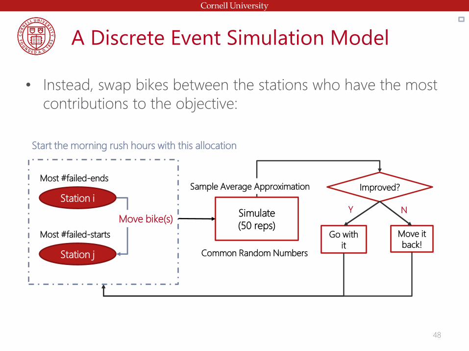
A Discrete Event Simulation Model
• Instead, swap bikes between the stations who have the most
contributions to the objective:
Simulate
(50 reps)
Improved?
Go with
it
Move it
back!
Start the morning rush hours with this allocation
Station i
Most #failed-ends
Station j
Most #failed-starts
Move bike(s)Y N
Sample Average Approximation
Common Random Numbers
48
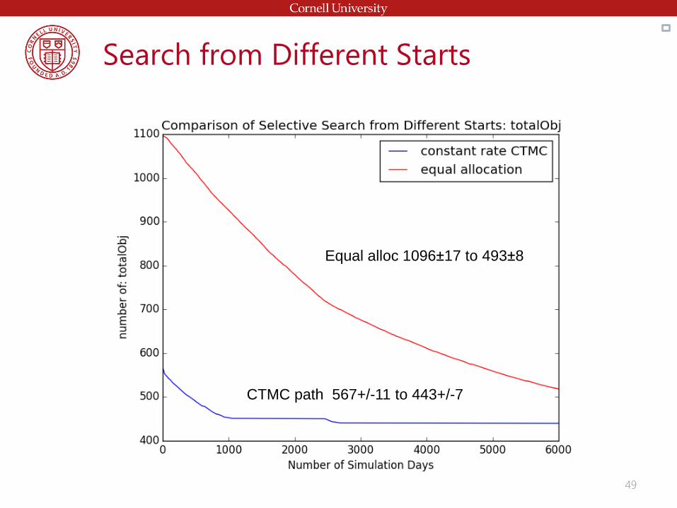
Search from Different Starts
CTMC path 567+/-11 to 443+/-7
Equal alloc 1096±17 to 493±8
49

Station Capacities
50
The size of the capacity at each station.
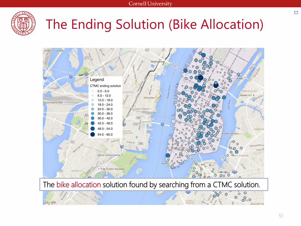
The Ending Solution (Bike Allocation)
51
The bike allocation solution found by searching from a CTMC solution.
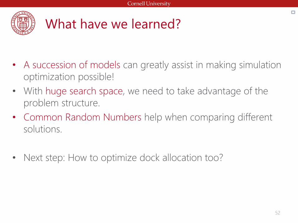
What have we learned?
• A succession of models can greatly assist in making simulation
optimization possible!
• With huge search space, we need to take advantage of the
problem structure.
• Common Random Numbers help when comparing different
solutions.
• Next step: How to optimize dock allocation too?
52

1. Introduction
2. Common Issues and Remedies
3. Tools
4. Case Study: Bike Sharing
Contents
53
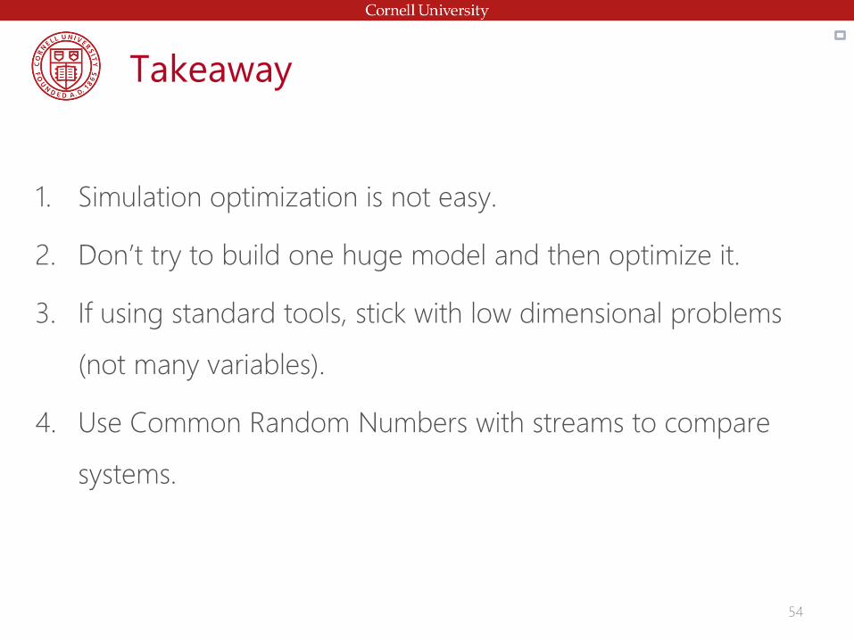
Takeaway
1. Simulation optimization is not easy.
2. Don’t try to build one huge model and then optimize it.
3. If using standard tools, stick with low dimensional problems
(not many variables).
4. Use Common Random Numbers with streams to compare
systems.
54
References
• Savage, S. 2015. “The Flaw of Averages”. Accessed Apr. 28, 2015. http://flawofaverages.com.
• Pasupathy, R. and S. G. Henderson 2012. “SimOpt”. Accessed Apr. 28, 2015. http://www.simopt.org.
• Fu, M. C. 2001. “Simulation Optimization”. In Proceedings of the 2001 Winter Simulation Conference, 53–61. Piscataway NJ: IEEE.
• Fu, M. C., F. W. Glover, and J. April. 2005. “Simulation Optimization: A Review, New Developments, and Applications”. In
Proceedings of the 37th Winter Simulation Conference, 83–95. Piscataway NJ: IEEE.
• Fu, M. C., C.-H. Chen, and L. Shi. 2008. “Some Topics for Simulation Optimization”. In Proceedings of the 40th Winter Simulation
Conference, 27–38. IEEE.
• Chau, M., M. C. Fu, H. Qu, and I. O. Ryzhov. 2014. “Simulation Optimization: A Tutorial Overview and Recent Developments in
Gradient-based Methods”. In Proceedings of the 2014 Winter Simulation Conference, edited by A. Tolk, D. Diallo, I. O. Ryzhov, L.
Yilmaz, S. Buckley, and J. A. Miller, 21–35. Piscataway NJ: IEEE.
• Banks, J., J. Carson, B. Nelson, and D. Nicol. 2010. Discrete-event system simulation. 5th ed. Prentice Hall.
• Fu, M. C. 2015. Handbook of Simulation Optimization. International Series in Operations Research & Management Science.
Springer New York.
• Hong, L., B. Nelson, and J. Xu. 2015. “Discrete Optimization via Simulation”. In Handbook of Simulation Optimization, edited by
M. C. Fu, Volume 216 of International Series in Operations Research & Management Science, 9–44. Springer New York.
• Kim, S., R. Pasupathy, and S. G. Henderson. 2015. “A Guide to Sample Average Approximation”. In Handbook of Simulation
Optimization, edited by M. C. Fu, Volume 216 of International Series in Operations Research & Management Science, 207–243.
New York: Springer.
• Barton, R. R. 2009. “Simulation Optimization Using Metamodels”. In Proceedings of the 2009 Winter Simulation Conference,
edited by M. D. Rossetti, R. R. Hill, B. Johansson, A. Dunkin, and R. G. Ingalls, 230–238. Piscataway NJ: IEEE.
• Kleijnen, J. P. C. 2015. “Response Surface Methodology”. In Handbook of Simulation Optimization, edited by M. C. Fu, Volume
216 of International Series in Operations Research & Management Science, 277–292. Springer New York.
55

References
• Chau, M., and M. C. Fu. 2015. “An Overview of Stochastic Approximation”. In Handbook of Simulation Optimization, edited by M.
C. Fu, Volume 216 of International Series in Operations Research & Management Science, 149–178. New York: Springer.
• Luo, J., and L. J. Hong. 2011. “Large-scale Ranking and Selection using Cloud Computing”. In Proceedings of the 2011 Winter
Simulation Conference, edited by S. Jain, R. R. Creasey, J. Himmelspach, K. P. White, and M. Fu, 4051–4061. Piscataway, NJ: IEEE.
• Luo, J., L. J. Hong, B. L. Nelson, and Y. Wu. 2014. “Fully Sequential Procedures for Large-scale Ranking-and-selection Problems in
Parallel Computing Environments”, accepted by Operations Research, forthcoming.
• Ni, E. C., D. F. Ciocan, S. G. Henderson, and S. R. Hunter. 2015. “Efficient Ranking and Selection in High Performance Computing
Environments”. Working paper.
• Chen, C., S. E. Chick, and L. H. Lee. 2015. “Ranking and Selection: Efficient Simulation Budget Allocation”. In Handbook of
Simulation Optimization, edited by M. C. Fu, Volume 216 of International Series in Operations Research & Management Science,
Chapter 3, 45–80. New York: Springer.
• Kim, S.-H., and B. L. Nelson. 2006. “Selecting the Best System”. In Simulation, edited by S. G. Henderson and B. L. Nelson,
Volume 13 of Handbooks in Operations Research and Management Science. Amsterdam: Elsevier.
• Andradóttir, S. 2015. “A Review of Random Search Methods”. In Handbook of Simulation Optimization, edited by M. C. Fu,
Volume 216 of International Series in Operations Research & Management Science, 277–292. Springer New York.
• Hong, L., B. Nelson, and J. Xu. 2015. “Discrete Optimization via Simulation”. In Handbook of Simulation Optimization, edited by
M. C. Fu, Volume 216 of International Series in Operations Research & Management Science, 9–44. Springer New York.
• Fu, M. C., F. W. Glover, and J. April. 2005. “Simulation Optimization: A Review, New Developments, and Applications”. In
Proceedings of the 37th Winter Simulation Conference, 83–95. Piscataway NJ: IEEE.
• Ólafsson, S. 2006. “Metaheuristics”. In Simulation, edited by S. G. Henderson and B. L. Nelson, Handbooks in Operations
Research and Management Science, 633–654. Amsterdam: Elsevier.
• O’Mahony, E., and D. B. Shmoys. 2015. “Data Analysis and Optimization for (Citi)Bike Sharing”. In Proceedings of the Twenty-
Ninth AAAI Conference on Artificial Intelligence, January 25-30, 2015, Austin, Texas, USA., 687–694. AAAI.
56

Index for Questions
• Introduction
– What is SO?
– SO is hard.
– The flaw of averages
– Formula
– Applications
– Scope and other references
• Common issues and remedies
– Local vs. global solutions
– Huge search space
– Continuous vs. discrete variables
– Optimizing in the presence of noise
– Simulation noise can swamp the signal (CRN)
– Failing to recognize an optimal solution
– Poor estimates of the optimal value
– When to stop
– Model madness58
• Tools
- Sample Average
Approximation
- Metamodeling
- Stochastic Approximation
and Gradient Estimation
- Ranking and Selection
- Random Search Methods
• Citibike
- Problem statement
- Half-full stations
- Fluid model
- CTMC
- Discrete event simulation
- Results