An Introduction to Quantum Mechanics:Exercises and Solutions

SERP-CHEM: 2011-15

Camillo Imbimbo

Dipartimento di Fisica dell’Universita di GenovaVia Dodecaneso, I-16136, Genova, Italia

Contents

1 The Failure of Classical Physics 21.1 Atom stability . . . . . . . . . . . . . . . . . . . . . . . . . . . 21.2 Equipartion theorem . . . . . . . . . . . . . . . . . . . . . . . 31.3 The Photoelectric Effect . . . . . . . . . . . . . . . . . . . . . 41.4 Bohr’s quantum theory of atomic spectra. . . . . . . . . . . . 51.5 Quantum theory of gas specific heat capacities . . . . . . . . . 10

1.5.1 Einstein and Debye theories of specific heat capacitiesof solids . . . . . . . . . . . . . . . . . . . . . . . . . . 10

2 The Principles of Quantum Mechanics 12

3 Simple systems 19

4 Time evolution 37

5 Symmetries 43

1 The Failure of Classical Physics

1.1 Atom stability

Exercise 1. Estimate the speed of the electron rotating around the nucleusfor the hydrogen atom, assuming that it orbitates alonga circular orbit ofradius r0 = 10−8 cm. Compare it to the speed of light.Solution.

v2 =e2

4 π ε0

1

mr0

≈ (1.6)2 × 10−38 9.0× 109 1

9.1× 10−31

1

1010

m2

sec2≈

≈ (1.6)2 0.99× 1012 m2

sec2(1.1)

Hence

v

c≈ 1.6× 106

3.0× 108= 0.53× 10−2 (1.2)

2

Exercise 2. Check that formula (1.7) of the lecture notes has the correctdimensions.Solution.

Recall that e2

4π ε0 r2 has the dimension of a force. Therefore

[ e2

4 π ε0

a2

c3

]=[M × L3

T 2

L2

T 4

T 3

L3

]=[M × L2

T 3

]=[ET

](1.3)

Exercise 3. Estimate the time that it takes an electron of the hydrogenatom to fall onto the nucleus, assuming it starts from a circular orbit of radiusr0 = 10−8 cm.Solution.

τ =(4 π ε0)2 c3m2

4 e4r3

0 =(4 π ε0mr0 c

2

e2

)2 r0

4 c=c4

v4

r0

4 c≈

≈ 1

0.534 × 10−8× 10−10

4× 3.0× 108sec ≈ 1.1 × 10−10 sec (1.4)

1.2 Equipartion theorem

Exercise 3. Prove that a mass m which is constrained to move freely on acircle on a plane by a rigid rod of radius R is described by an Hamiltonian ofthe form

H(p, θ) =p2θ

2 I(1.5)

where pθ is the momentum conjugate to angle θ which measures the positionof the particle on the circle, and I is called the momentum of inertia. ExpressI in terms of m and R.Solution.

The velocity of the particle is

v = Rd θ

d t(1.6)

Therefore its energy is

H =1

2mv2 =

1

2mR2 θ2 (1.7)

3

The momentum conjugate to θ is

pθ = mR2θ (1.8)

Thus

H =1

2

p2θ

mR2(1.9)

Thus

I = mR2 (1.10)

Exercise 4. Prove that a diatomic molecule schematized as two identicalmasses m

2held at a fixed distance R by a rigid rod of negligible mass is

described by the Hamiltonian

H(p, q) =~p2

2m+

1

2 I

(p2θ +

p2φ

sin2 θ

)(1.11)

Compute the momentum of inertia I in terms of m and R.Problem 2. Generalize the derivation of the equipartition theorem to theHamiltonian of the bi-atomic molecule (1.11).

1.3 The Photoelectric Effect

Problem 5. A lamp of 100 W emits light whose wave length is 5.890 10−7m.How many photons are emitted in 1 second?Solution The energy of photons of such frequency is

Eν =12400

5890eV = 2.10 eV = 3.37× 10−19J (1.12)

Therefore the number dNdt

of photons emitted per unit of time is

dN

dt=

100W

3.37 10−19J= 2.97× 1020 sec−1 (1.13)

4

1.4 Bohr’s quantum theory of atomic spectra.

Problem 6. Classical electromagnetism predicts that a charge rotating on acircular orbit with angular orbital frequency ω emits electromagnetic radiationwith the same frequency. Show that the frequency of the photon emitted byan electron of the Bohr hydrogen atom which goes from the level EH

n+1 to thelevel EH

n , is, for n large, approximately equal to the frequency of the classicalcircular motion corresponding to that energy.Solution: The difference of energy of the levels EH

n+1 and EHn for n >> 1 is

EHn+1 − EH

n = − e4m

(4π ε0)2 ~2

1

2 (n+ 1)2+

e4m

(4 π ε0)2 ~2

1

2n2=

≈ e4m

(4 π ε0)2 ~2

1

n3(1.14)

The angular frequency of the corresponding emitted photon is

ωn+1→n =e4m

(4 π ε0)2 ~3

1

n3(1.15)

On the other hand, the angular frequency for a classical circular orbit ofradius r is

ω =v

r(1.16)

Since

v2 =e2

4 π ε0m

1

r(1.17)

we have

ω =4π ε0e2

mv3 (1.18)

The velocity vn of the electron in the circular orbit of energy En is given by

En = −1

2mv2

n = − e4m

(4π ε0)2 ~2

1

2n2(1.19)

that is

vn =1

n

e2

(4 π ε0) ~(1.20)

5

The angular frequency of the circular orbit with this energy is therefore

ω = v3n

4 π ε0e2

m =1

n3

e4m

(4 π ε0)2 ~3(1.21)

which matches the frequency of the photon emitted in the transition n+1→ nas predicted by Bohr theory.Problem 9. Apply the Bohr-Sommerfeld quantization condition to anunidimensional free particle moving in a potential well V (x) defined by

V (x) =

{−V0 for 0 < x < L

0 for x < 0 and x > L(1.22)

where V0 > 0 is the depth of the well. Determine the discrete energy levels.How many they are? What is the minimum value of V0 for which there existdiscrete levels?Solution: The bound classical trajectories are those with E < 0. Themomentum for these orbits is quantized according to

pn =nh

2L(1.23)

The energy is therefore

En =p2n

2m− V0 =

n2 h2

8mL2− V0 < 0 (1.24)

Hence there are a finite number of closed trajectories, with n = 1, 2, . . . nmaxwhere nmax is the highest positive integer such that

n2max <

8mL2 V0

h2(1.25)

The minimal value of V0 for which there are discrete levels is the minimalvalue for which this equation admits an integer positive solution

8mL2 V min0

h2= 1⇔ V min

0 =h2

8mL2(1.26)

Problem 10. Apply Bohr-Sommerfeld quantization condition to a satelliteof mass m = 1 kg rotating around the earth. Determine the allowed radiusesin terms of the mass of the earth M and the universal constant of gravitation

6

G. Suppose the satellite is on on circular orbit of radius near the radius ofthe earth R = 6400 km, with a given Bohr integer number n. How much doesthe radius change if the satellite shifts to an orbit with n = n+ 1? Expressthe answer in meters.Solution: The classical equation of motion for a circular orbit of radius r is

GM

r2=v2

r⇔ v2 =

GM

r(1.27)

The momentum is therefore

p = mv = m

√GM

r(1.28)

and the Bohr-Sommerfeld quantization condition is∮p dr = 2π r p = 2πm

√GM r = nh (1.29)

that is

rn =n2 ~2

GM m2(1.30)

If n changes from n→ n+ ∆n = n+ 1 the radius changes

∆rn = rn+1 − rn ≈2n∆n ~2

GM m2=

2 ∆n rnn

=2 rnn

(1.31)

We have

rn =n2 ~2

GM m2≈ R⇔ n2 ≈ GM Rm2

~2=g m2R3

~2(1.32)

where g = GMR2 ≈ 9.8 m

sec2is the gravity acceleration. Thus

n2 ≈ 9.8× 12 × 6.43 × 1018

1.052 × 10−68≈ 24× 1088 ⇒ n ≈ 5× 1044 (1.33)

Then

∆rn ≈2

5× 1044× 6.4× 106m ≈ 2.6× 10−38m (1.34)

7

Problem 12. Apply the Bohr-Sommerfeld quantization condition to computethe energy levels and the orbits of a particle of mass m moving in circularorbits of radius r in a potential V (r) = σ r.Solution: The classical equation of motion is

mv2

r= σ (1.35)

The quantization condition on the angular momentum for a circular orbit ofradius r is therefore

L = mr v = mr

√σ r

m=√mσ r

32 = n ~ (1.36)

The orbits have therefore radiuses

rn =(n ~)

23

(mσ)13

(1.37)

and the corresponding energies are

En =3

2σ rn =

3

2

(n ~σ)23

m13

(1.38)

Problem 13. Apply the Bohr-Sommerfeld quantization condition to deriveenergy levels and allowed orbit radiuses for a particle of mass m moving incircular orbits of radius r attracted toward the center of the orbit by an elasticforce F = −k r.Solution: The classical equations of motion for circular orbits are

mv2

r= k r (1.39)

Therefore

v2 =k

mr2 ⇒ v =

√k

mr ≡ ω r (1.40)

where ω =√

km

is the angular frequency of the harmonic oscillations. The

angular momentum of the circular orbit is therefore

L = mv r = mω r2 (1.41)

8

and the Bohr quantization condition Ln = n ~ gives for the radiuses of thecircular orbits

r2n =

n ~mω

(1.42)

The corresponding energy levels are therefore

En =1

2mv2

n +1

2mω2 r2

n =1

2mω2 r2

n +1

2mω2 r2

n =

= mω2 r2n = n ~ω (1.43)

Problem 14. Derive the numerical values for the Rydberg constants pre-dicted by Bohr atomic model for the following hydrogenoids: hydrogen H,deuteron D (whose nucleus has one proton and one neutron), He+, Li++ and,for the same elements, the wave lengths of the spectral lines corresponding tothe transition between the first excited level and the fundamental level.Solution:

Let us denote by R∞ the Rydberg constant for an infinitely massivenucleus

R∞ =( e2

4 π ε0

)2 1

4π

me

~3 c≈ 109737 cm−1 (1.44)

The Rydberg constant R(M) for a nucleus of mass M and charge Z is relatedto the energy levels by the formula

En = −Z2 R(M)h c

n2(1.45)

a

R(M) = R∞1

1 + meM

≈ R∞(1− me

M

)(1.46)

Recall that

mp

me

= 1836.15 (1.47)

9

Therefore

RH = R(mp) ≈ R∞(1− me

mp

)= 109677 cm−1

RD = R(2 ∗mp) ≈ R∞(1− me

2mp

)= 109707 cm−1

RHe+ = R(4 ∗mp) ≈ R∞(1− me

4mp

)= 109722 cm−1

RLi++ = R(7 ∗mp) ≈ R∞(1− me

7mp

)= 109728 cm−1 (1.48)

The wave lengths of the first spectral line corresponding to the transitionfrom n = 1 to n = 2 are

λH =4

3

1

RH

= 1215.69 A

λD =4

3

1

RD

= 1215.36 A

λHe+ =4

3

1

4RHe+= 303.798 A

λLi++ =4

3

1

9RLi++

= 135.013 A (1.49)

1.5 Quantum theory of gas specific heat capacities

1.5.1 Einstein and Debye theories of specific heat capacities ofsolids

Problem 16. Suppose that the density of states of phonons grows quadrati-cally with the frequency

dn(ω)

dω= Aω2 +O(ω3) for ω � ωmax (1.50)

only for small frequencies ω. n(ω) is an otherwise generic function of ω forbigger ω up to a certain given ωmax, which defines a Debye temperature TD.Derive the predictions of the Debye model for the internal energy in the lowand high temperature limit.Solution:

Let us start from

U =

∫ ωmax

0

dω n′(ω)~ω e−β ~ω

1− e−β ~ω (1.51)

10

For T � TD ≡ ~ωmaxk

,

~ β ω ≤ ~ β ωmax � 1 (1.52)

Therefore the high temperature limit of the internal energy coincides withthe classical result, as expected on general grounds

U ≈∫ ωmax

0

dω n′(ω)~ωβ ~ω

=1

β

∫ ωmax

0

dω n′(ω) =3NA

βT � TD (1.53)

On the other hand for low temperatures, when T � TD,

1

~ β� ωmax (1.54)

the integrand in (1.51) is significantly different than zero only if

ω .1

~ β� ωmax (1.55)

Therefore, in the region of frequencies when the integrand is significantlydifferent than zero we can approximate the density of state with (1.50) and

U ≈ A

∫ ωmax

0

dω~ω3 e−β ~ω

1− e−β ~ω ≈A ~

(~ β)4

∫ ∞0

dxx3 e−x

1− e−x=

=A

~3

π4

15

1

β4(1.56)

In the lecture notes we derived the expression of A in terms of the soundspeed in the solid and the volume

A =3L3

2π2 v3(1.57)

Therefore

U ≈ L3

v3 ~3

π2

10k4 T 4 T � TD (1.58)

Problem 17. Discuss the effect of quantization on the specific heat capacitiesof bi-atomic gases, knowing that: a) the rotational degrees of freedom aroundan axis orthogonal to the axis connecting the two atoms give rise to discreteenergy levels with separation ∆E ∼ 10−4 − 10−2 eV ; b) vibrational degreesof freedom have ∆E ∼ 10−1 eV ; c) rotational degrees of freedom around theaxis connecting the two atoms have ∆E ∼ 10 eV .Solution. TO BE GIVEN

11

2 The Principles of Quantum Mechanics

Problem 10. A system is described by a 2-dimensional space of states. Let|1〉 and |2〉 be the normalized eigenstates of an observable O with eigenvaluesλ = 1 and λ = 2 respectively. Let v = |1〉+ i

√3|2〉 be a state of the system.

a) What is the probability that the measure of O on v gives the resultλ = 2?

b) Write the 2× 2 matrix which represents O in the basis {|1〉, |2〉}.c) Let O′ be another observable, such that O′|1〉 = |2〉 and O′|2〉 = |1〉.

Write the 2× 2 matrix which represents O′ in the basis {|1〉, |2〉}.d) What are the eigenvalues of O′?e) What is the average of O′ on the state v?

Solution:

• a) Let us compute the norm of v

|v|2 = 1 + |i√

3|2 = 1 + 3 = 4 (2.1)

Thus the normalized vector

v′ =1

2

(|1〉+ i

√3|2〉

)(2.2)

describes the same physical state as v. From (2.2) we read the proba-bilities

Pλ=1(v) =∣∣∣12

∣∣∣2 =1

4Pλ=2(v) =

∣∣∣i√3

2

∣∣∣2 =3

4(2.3)

• b) Since {|1〉, |2〉} are the eigenstates of O, in this basis O is representedby a diagonal matrix

O =

(1 00 2

)(2.4)

• c) The matrix representing O′ in the basis {|1〉, |2〉} is

O′ =(

0 11 0

)(2.5)

12

• d) The eigenvalues of O′ are obtained from the secular equation

det

(−λ′ 1

1 −λ′)

= (λ′)2 − 1 = 0⇔ λ′ = 1,−1 (2.6)

• e) The average of O′ on v is

〈v′,O′ v′〉 = 〈v′,O′ 12

(|1〉+ i

√3|2〉

)〉 =

= 〈v′, 1

2

(|2〉+ i

√3|1〉

)〉 =

= 〈12

(|1〉+ i

√3|2〉, 1

2

(|2〉+ i

√3|1〉

)〉 =

=1

4

(i√

3− i√

3)

= 0 (2.7)

Problem 11. On a spin 1/2 system the following 3 observables are defined

Sz =~2

(1 00 −1

)Sx =

~2

(0 11 0

)Sy =

~2

(0 −ii 0

)(2.8)

a) Find the eigenvalues and the normalized eigenvectors of the 3 observables{Sx, Sy, Sz}.

b) Suppose the system is in the state described by the vector

v =

(13 i

)(2.9)

Find the probabilities to obtain the various possible values of {Sx, Sy, Sz} onv. (You should in other words compute 6 probabilities, 2 for each of the 3observables.)

c) Compute the 2x2 unitary matrix which connects the basis of eigenvectorsof Sz with the basis of eigenvectors of Sy.

d) Find the eigenvalues and the normalized eigenvectors of the observable

S~n ≡ nx Sx + ny Sy + nz Sz (2.10)

where

~n = (nx, ny, nz) = (sin θ cosφ, sin θ sinφ, cos θ) (2.11)

13

θ and φ are polar coordinates: 0 ≤ φ ≤ 2 π and 0 ≤ θ ≤ π.e) Compute the 2x2 unitary matrix which connects the basis of eigenvectors

of Sz with the basis of eigenvectors of S~n.Solution:

a) The eigenvalues of any of {Sx, Sy, Sz} are

λ± = ±~2

(2.12)

The eigenvectors of Sx are obtained from(0 11 0

)(x±y±

)= ±

(x±y±

)(2.13)

that is

|Sx = ±~2〉 =

1√2

(1±1

)(2.14)

The eigenvectors of Sy are obtained from(0 −ii 0

)(x±y±

)= ±

(x±y±

)(2.15)

that is

|Sy = ±~2〉 =

1√2

(1±i

)(2.16)

Finally, yhe eigenvectors of Sz are obtained from(1 00 −1

)(x±y±

)= ±

(x±y±

)(2.17)

that is

|Sz =~2〉 =

1√2

(10

)|Sz = −~

2〉 =

1√2

(01

)(2.18)

b) Let us consider the normalized vector

|v〉 =1√10

(13 i

)(2.19)

14

The transition amplitudes are given by the scalar products

〈Sx =~2|v〉 =

1√20

(1 + 3 i)

〈Sy =~2|v〉 =

1√20

(1 + 3) =1√20

4

〈Sz =~2|v〉 =

1√10

(2.20)

The corresponding probabilities are therefore∣∣〈Sx =~2|v〉∣∣2 =

1

20|1 + 3 i|2 =

1

2∣∣〈Sy =~2|v〉∣∣2 =

16

20=

4

5∣∣〈Sz =~2|v〉∣∣2 =

1

10(2.21)

Hence the other probabilities are therefore∣∣〈Sx = −~2|v〉∣∣2 = 1− 1

2=

1

2∣∣〈Sy = −~2|v〉∣∣2 = 1− 4

5=

1

5∣∣〈Sz = −~2|v〉∣∣2 = 1− 1

10=

9

10(2.22)

c)

|Sy =~2〉 =

1√2

(1i

)=

1√2|Sz =

~2〉+

i√2|Sz = −~

2〉

|Sy = −~2〉 =

1√2

(1−i

)=

1√2|Sz =

~2〉 − i√

2|Sz = −~

2〉 (2.23)

The unitary matrix is therefore

U =1√2

(1 1i −i

)(2.24)

d) The matrix

S~n = Sx =~2

(nz nx − iny

nz + iny nz

)(2.25)

15

has eigenvalues

λ± = ±~2

(2.26)

The eigenvectors are obtained from(nz nx − i ny

nx + i ny −nz

)(x±y±

)= ±

(x±y±

)(2.27)

that is

nz x± + (nx − i ny)y± = ±x± (2.28)

Hence

|S~n = ±~2〉 =

1√2(1∓ nz)

(nx − i ny±1− nz

)=

1√2(1∓ cos θ)

(sin θ e−i φ

±1− cos θ

)Therefore

|S~n =~2〉 =

(cos θ

2e−i φ

sin θ2

)|S~n = −~

2〉 =

(sin θ

2e−i φ

− cos θ2

)(2.29)

e)

U =

(cos θ

2e−i φ sin θ

2e−i φ

sin θ2

− cos θ2

)(2.30)

Problem 13. Show that

v~p0,∆(~x) =

∫d3~p v~p(~x)φ~p0,∆(~p) (2.31)

with

v~p(~x) =ei~~x·~p

(2 π ~)32

φ~p0,∆(~p) =1

(π)34 ∆

32

e−(~p−~p0)2

2 ∆2 (2.32)

is a normalizable wave function of unit norm. Compute the average of ~x, ~p∆p2 and ∆x2 on the state described by the packet (2.31). Make use of theformula for gaussian integrals∫ ∞

−∞dx e−αx

2+β x =

√π

αeβ2

4α (2.33)

16

where α > 0 and β is a generic complex number.

Solution: Let us compute the norm of this vector in the momentum represen-tation

〈v, v〉 =

∫d3~p∣∣φ~p0,∆)(~p)

∣∣2 =

∫d3~p

(π)32 ∆3

e−(~p−~p0)2

∆2 =

=

∫d3~p

(π)32 ∆3

e−~p2

∆2 =1

(π)32 ∆3

π32 (∆2)

32 = 1 (2.34)

Let us compute the average of ~x in the momentum representation

〈v, ~x v〉 =

∫d3~p

(π)32 ∆3

e−(~p−~p0)2

2 ∆2 i ~ ~∇~p e−(~p−~p0)2

2 ∆2 =

= −i ~∫

d3~p

(π)32 ∆3

e−(~p−~p0)2

∆2 × (~p− ~p0)

∆2=

= −i ~∫

d3~p

(π)32 ∆3

e−~p2

∆2 × ~p

∆2= 0 (2.35)

Let us compute the average of ~p in the momentum representation

〈v, ~p v〉 =

∫d3~p

(π)32 ∆3

e−(~p−~p0)2

2 ∆2 ~p e−(~p−~p0)2

2 ∆2 =

=

∫d3~p

(π)32 ∆3

e−~p2

∆2 (~p+ ~p0) = ~p0 (2.36)

Let us compute the average of ~x2 in the momentum representation

〈v, ~x2 v〉 = −∫

d3~p

(π)32 ∆3

e−(~p−~p0)2

2 ∆2 ~2 ~∇2~p e−

(~p−~p0)2

2 ∆2 =

= +~2

∫d3~p

(π)32 ∆3

e−(~p−~p0)2

2 ∆2 × ~∇~p

[(~p− ~p0)

∆2e−

(~p−~p0)2

2 ∆2

]=

= +~2

∫d3~p

(π)32 ∆3

e−(~p−~p0)2

∆2 ×[−(~p− ~p0)2

∆4+

3

∆2

]=

= +3 ~2

∆2− ~2

∫d3~p

(π)32 ∆3

e−~p2

∆2~p2

∆4(2.37)

17

Integrals like those which appear in the r.h.s. can be computed in the followingway ∫

d3~x e−α~x2

~x2 = −∂α∫d3~x e−α~x

2

= −∂απ

32

α32

=3

2

π32

α52

(2.38)

Hence

〈v, ~x2 v〉 = +3 ~2

∆2− 3

2

~2

∆2=

3 ~2

2 ∆2(2.39)

Therefore the uncertainty on ~x2 is

∆~x2 = 〈v, ~x2 v〉 − 〈v, ~x v〉2 =3 ~2

2 ∆2(2.40)

Let us compute the average of ~p2

〈v, ~p2 v〉 =

∫d3~p

(π)32 ∆3

e−(~p−~p0)2

2 ∆2 ~p2 e−(~p−~p0)2

2 ∆2 =

=

∫d3~p

(π)32 ∆3

e−~p2

∆2 (~p+ ~p0)2 =

= ~p20 +

3

2∆2 (2.41)

Therefore the uncertainty on the ~p2 is

∆~p2 = 〈v, ~p2 v〉 − 〈v, ~p v〉2 =3

2∆2 (2.42)

Note that

√∆~x2

√∆~p2 =

3

2~ (2.43)

Since the state is rotation invariant

∆~x2 = ∆(x2 + y2 + z2) = 3 ∆x2

∆~p2 = ∆(p2x + p2

y + p2z) = 3 ∆p2

x (2.44)

Therefore

∆x×∆px = ∆y ×∆py = ∆z ×∆pz =~2

(2.45)

18

The state considered is therefore a state of minimal uncertainty.The same computation could be done in the Schrodinger representation.

Let us first compute the wave function in the Schrodinger representation

v~p0,∆(~x) =1

(2 ~π)32

∫d3~p e

i~ ~p·~x

1

(π)34 ∆

32

e−(~p−~p0)2

2 ∆2 =

=ei~ ~p0·~x

(2 ~π)32

∫d3~p

1

(π)34 ∆

32

ei~ ~p·~x−

~p2

2 ∆2 =

=ei~ ~p0·~x

(2 ~π)32

∫d3~p

1

(π)34 ∆

32

e−(~p− i~ ∆2 ~x)2

2 ∆2 × e−∆2 ~x2

2 ~2 =

=(∆

~

) 32 e

i~ ~p0·~x

(π)34

e−∆2 ~x2

2 ~2 (2.46)

The averages of ~x and ~p are

〈v, ~x v〉 =(∆

~

)3 1

π32

∫d3~x e−

∆2 ~x2

~2 ~x = 0

〈v, ~p v〉 =(∆

~

)3 1

π32

∫d3~x e−

∆2 ~x2

~2

[i

∆2 ~x

~+ ~p0

]= ~p0 (2.47)

The averages of ~x and ~p write

〈v, ~x2 v〉 =(∆

~

)3 1

π32

∫d3~x e−

∆2 ~x2

~2 ~x2 =3 ~2

2 ∆2

〈v, ~p2 v〉 =(∆

~

)3 1

π32

∫d3~x e−

∆2 ~x2

~2

[3 ∆2 + ~p2

0 −∆4 ~x2

~2

]=

= ~p20 + 3 ∆2 − 3

2∆2 = ~p2

0 +3

2∆2 (2.48)

in agreements with the results obtained above in the momentum representa-tion.

3 Simple systems

Problem 3. Show that the exponential factor which controls the probabilityof tunneling through the barrier

V (x) =

+∞ if x < 0,

−V0 if 0 < x < LZ e2

4π ε0 xif x > L

(3.1)

19

in the limit

E � Z e2

4 π ε0 L(3.2)

is

T ∝ e− π Z e2

4π ε0 ~

√2mE = e

− Z e2

2 ε0 ~ v (3.3)

Solution:Let us compute the integral∫ Z e2

4π ε0 E

L

dx

√Z e2

4π ε0 x− E =

Z e2

4π ε0√E

∫ 1

4π ε0 LE

Z e2

dy√y

√1− y (3.4)

In the limit (3.2)∫ 1

4π ε0 LE

Z e2

dy√y

√1− y →

∫ 1

0

dy√y

√1− y =

∫ 1

0

2 dξ√

1− ξ2 =π

2(3.5)

Hence

T ∝ e−2

√2m~2

Z e2

4π ε0√E

π2 = e

−π√

2mE

Z e2

4π ε0 ~ = e− Z e2

2 ε0 ~ v (3.6)

Problem 5. Find the reflection and transmission coefficients R and T forthe rectangular potential barrier for E < V0, in the limit in which L → 0,V0 → +∞ and V0 L = V constant. (This is the so-called “thin barrier” limit.)Solution:

In this limit

L→ 0 Lk′ →√

2mV~

√L→ 0 (k′)2 L→ 2mV

~2(3.7)

Then

T =16 k2 |k′|2∣∣(k + i |k′|)2 e−|k′|L − (k − i |k′|)2 e|k′|L

∣∣2 =

=16 k2 |k′|2∣∣∣(k2 − |k′|2

) (e−|k′|L − e|k′|L

)+ 2 i k |k′|

(e−|k′|L + e|k′|L

)∣∣∣2→ 16 k2 |k′|2∣∣∣|k′|2 2 |k′|L+ 2 i k |k′| 2

∣∣∣2 =4 k2∣∣|k′|2 L+ 2 i k

∣∣2 →→ k2∣∣mV

~2 + i k∣∣2 =

~2 k2

m2 V2

~2 + ~2 k2=

p2

m2 V2

~2 + p2(3.8)

20

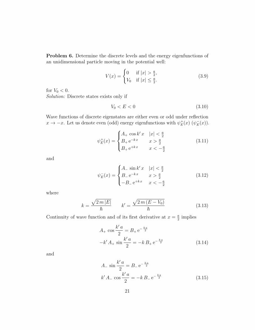
Problem 6. Determine the discrete levels and the energy eigenfunctions ofan unidimensional particle moving in the potential well:

V (x) =

{0 if |x| > a

2,

V0 if |x| ≤ a2.

(3.9)

for V0 < 0.Solution: Discrete states exists only if

V0 < E < 0 (3.10)

Wave functions of discrete eigenstates are either even or odd under reflectionx→ −x. Let us denote even (odd) energy eigenfunctions with ψ+

E(x) (ψ−E(x)).

ψ+E(x) =

A+ cos k′ x |x| < a

2

B+ e−k x x > a2

B+ e+k x x < −a2

(3.11)

and

ψ−E(x) =

A− sin k′ x |x| < a

2

B− e−k x x > a2

−B− e+k x x < −a2

(3.12)

where

k =

√2m |E|~

k′ =

√2m (E − V0)

~(3.13)

Continuity of wave function and of its first derivative at x = a2

implies

A+ cosk′ a

2= B+ e−

k a2

−k′A+ sink′ a

2= −k B+ e−

k a2 (3.14)

and

A− sink′ a

2= B− e−

k a2

k′A− cosk′ a

2= −k B− e−

k a2 (3.15)

21

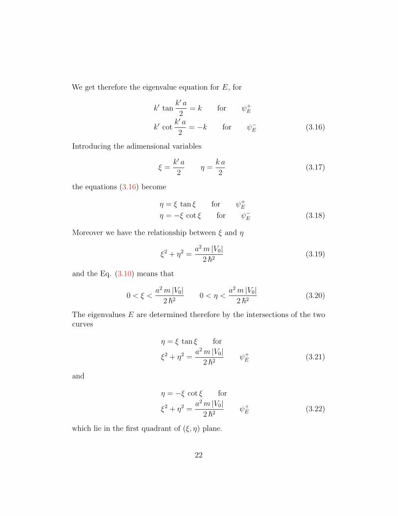
We get therefore the eigenvalue equation for E, for

k′ tank′ a

2= k for ψ+

E

k′ cotk′ a

2= −k for ψ−E (3.16)

Introducing the adimensional variables

ξ =k′ a

2η =

k a

2(3.17)

the equations (3.16) become

η = ξ tan ξ for ψ+E

η = −ξ cot ξ for ψ−E (3.18)

Moreover we have the relationship between ξ and η

ξ2 + η2 =a2m |V0|

2 ~2(3.19)

and the Eq. (3.10) means that

0 < ξ <a2m |V0|

2 ~20 < η <

a2m |V0|2 ~2

(3.20)

The eigenvalues E are determined therefore by the intersections of the twocurves

η = ξ tan ξ for

ξ2 + η2 =a2m |V0|

2 ~2ψ+E (3.21)

and

η = −ξ cot ξ for

ξ2 + η2 =a2m |V0|

2 ~2ψ+E (3.22)

which lie in the first quadrant of (ξ, η) plane.

22

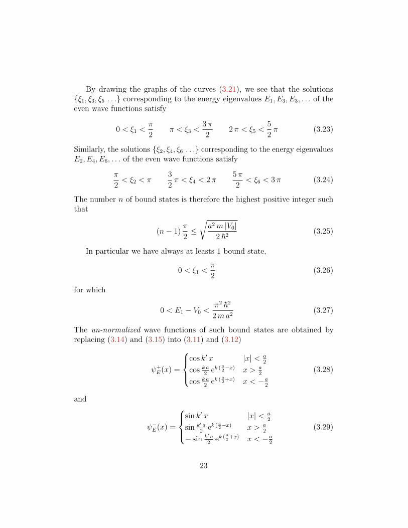
By drawing the graphs of the curves (3.21), we see that the solutions{ξ1, ξ3, ξ5 . . .} corresponding to the energy eigenvalues E1, E3, E3, . . . of theeven wave functions satisfy

0 < ξ1 <π

2π < ξ3 <

3π

22π < ξ5 <

5

2π (3.23)

Similarly, the solutions {ξ2, ξ4, ξ6 . . .} corresponding to the energy eigenvaluesE2, E4, E6, . . . of the even wave functions satisfy

π

2< ξ2 < π

3

2π < ξ4 < 2π

5 π

2< ξ6 < 3 π (3.24)

The number n of bound states is therefore the highest positive integer suchthat

(n− 1)π

2≤√a2m |V0|

2 ~2(3.25)

In particular we have always at leasts 1 bound state,

0 < ξ1 <π

2(3.26)

for which

0 < E1 − V0 <π2 ~2

2ma2(3.27)

The un-normalized wave functions of such bound states are obtained byreplacing (3.14) and (3.15) into (3.11) and (3.12)

ψ+E(x) =

cos k′ x |x| < a

2

cos k a2

ek (a2−x) x > a

2

cos k a2

ek (a2

+x) x < −a2

(3.28)

and

ψ−E(x) =

sin k′ x |x| < a

2

sin k′ a2

ek (a2−x) x > a

2

− sin k′ a2

ek (a2

+x) x < −a2

(3.29)

23

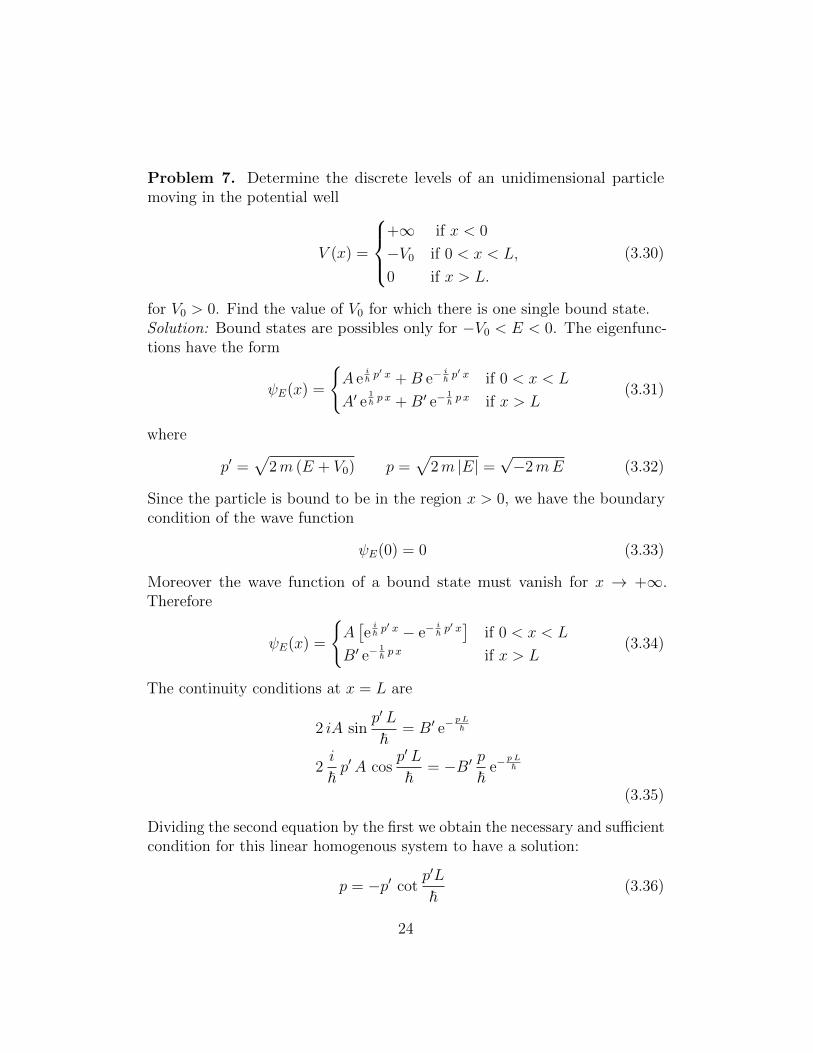
Problem 7. Determine the discrete levels of an unidimensional particlemoving in the potential well

V (x) =

+∞ if x < 0

−V0 if 0 < x < L,

0 if x > L.

(3.30)

for V0 > 0. Find the value of V0 for which there is one single bound state.Solution: Bound states are possibles only for −V0 < E < 0. The eigenfunc-tions have the form

ψE(x) =

{A e

i~ p′ x +B e−

i~ p′ x if 0 < x < L

A′ e1~ p x +B′ e−

1~ p x if x > L

(3.31)

where

p′ =√

2m (E + V0) p =√

2m |E| =√−2mE (3.32)

Since the particle is bound to be in the region x > 0, we have the boundarycondition of the wave function

ψE(0) = 0 (3.33)

Moreover the wave function of a bound state must vanish for x → +∞.Therefore

ψE(x) =

{A[ei~ p′ x − e−

i~ p′ x]

if 0 < x < L

B′ e−1~ p x if x > L

(3.34)

The continuity conditions at x = L are

2 iA sinp′ L

~= B′ e−

pL~

2i

~p′A cos

p′ L

~= −B′ p

~e−

pL~

(3.35)

Dividing the second equation by the first we obtain the necessary and sufficientcondition for this linear homogenous system to have a solution:

p = −p′ cotp′L

~(3.36)

24

Energy eigenvalues are therefore determined by the intersections of the twocurves in the positive quadrant of the (p′, p) plane

p = −p′ cotp′ L

~p′2 + p2 = 2mV0

p > 0 p′ > 0 (3.37)

Introducing the adimensional variables

ξ =p′ L

~η =

pL

~α2 ≡ 2mV0 L

2

~2(3.38)

the equations of the curves become

η = −ξ cot ξ

ξ2 + η2 = α2

η > 0 η > 0 (3.39)

Drawing the graphs of the two curves we see that minimal α for which anintersection in the positive quadrant exists is for α = π

2

α =π

2ξ =

π

2η = 0 (3.40)

Thus the minimal value of V0 for which there is a bound state is

V min0 =

~2 π2

8mL2(3.41)

When α increases and

π

2< α <

3 π

2(3.42)

there is one single intersection in the positive quadrant. Thus for

~2 π2

8mL2< V0 <

9 ~2 π2

8mL2(3.43)

there is a single bound state with

E0 =~2 ξ

2mL2− V0

π

2< ξ < π (3.44)

25

More generally when α reaches the values

αn =π

2,3 π

2,5 π

2, . . . (3.45)

new solutions with η = 0 appear, in correspondence with new bound states.The new bound states starts at E = 0 for α = αn, and, as α goes from αn toαn+1, its energy becomes more negative and lies in the range

α2n ~2

2mL2− V0 < E <

α2n+1 ~2

2mL2− V0 (3.46)

When V0 →∞ the numbers of bound states increases. The ground statelevel E0 tends to the limiting value

E0 =~2 ξ

2mL2− V0 →

~2 π2

2mL2− V0 (3.47)

Problem 8. Determine the discrete levels of an unidimensional particlemoving in the potential well by using the expression obtained for the transfermatrix for the potential barrier

T =1

4×

×

((k+k′)2

k k′ei (k−k

′)L − (k−k′)2

k k′ei (k+k′)L k2−(k′)2

k k′

(e−i (k−k

′)L − e−i (k+k′)L)

k2−(k′)2

k k′

(ei (k−k

′)L − ei (k+k′)L) (k+k′)2

k k′e−i (k−k

′)L − (k−k′)2

k k′e−i (k+k′)L

)

Solution:We must put in this case

k =

√2mE

~= i

√2m |E|~

= i |k| k′ =

√2m (E + V0)

~(3.48)

Moreover we should impose

A = B′′ = 0 A′′ = 1 (3.49)

in the equation (AB

)= T

(A′′

B′′

)(3.50)

26

Hence the equation which determine the energy levels is

T11 =(i |k|+ k′)2

k k′ei (k−k

′)L − (i |k| − k′)2

k k′ei (k+k′)L = 0 (3.51)

from which

(i |k|+ k′)2

(i |k| − k′)2= e2 i k′ L (3.52)

Let us put

i |k|+ k′ =∣∣i |k|+ k′

∣∣ ei θE tan θE =|k|k′

(3.53)

Thus

(i |k|+ k′)2

(i |k| − k′)2= e4 i θE (3.54)

The equations for the eigenvalues becomes therefore

4 θE = 2k′ L+ 2nπ n = 0,±1,±2, . . . (3.55)

i.e.

θE =k′ L

2+nπ

2⇒ tan θE =

|k|k′

= tan(k′ L

2+nπ

2) (3.56)

For n even

|k|k′

= tan(k′ L

2) (3.57)

and for n odd

−|k|k′

= cot(k′ L

2) (3.58)

in agreement with (3.16).Problem 9. Determine the energy eigenfunctions for the potential barrier

V (x) =

{0 if |x| > a

2,

V0 if |x| ≤ a2.

(3.59)

27

with V0 > 0 and 0 < E < V0 which are also eigenstates of the spatial inversionoperator I : ψ(x)→ ψ(−x). Derive the transmission matrix for this barrier.Solution:

The even and odd energy eigenfunctions with 0 < E < V0 have the form:

ψ+E(x) =

e+i k x +B+e−i k x x < −a

2

A+ cosh k′ x |x| < a2

B+ei k x + e−i k x x > a2

(3.60)

and

ψ−E(x) =

e+i k x +B−e−i k x x < −a

2

A− sinh k′ x |x| < a2

−B−ei k x − e−i k x x > a2

(3.61)

where

k =

√2mE

~k′ =

√2m |V0 − E|

~(3.62)

Continuity of the wave-functions and of their first derivative at x = ±a2

gives

B+ e+i k a2 + e−i

k a2 = A+ cosh

k′ a

2

i k(B+ei

k a2 − e−i

k a2

)= A+ k

′ sinhk′ a

2

B− eik a2 + e−i

k a2 = −A− sinh

k′ a

2

−i k(B−ei

k a2 − e−i

k a2

)= A+ k

′ cosk′ a

2(3.63)

From this

B+ − e−i k a

B+ + e−i k a= −ik

′

ktanh

k′ a

2

B− − e−i k a

B− + e−i k a= −i k

′

kcoth

k′ a

2(3.64)

and

B+ =1 + i k

′

ktanh k′ a

2

1− i k′k

tanh k′ a2

e−i k a = e2 i θ+(E) e−i k a

B− =1 + i k

′

kcoth k′ a

2

1− i k′k

coth k′ a2

e−i k a = e2 i θ−(E) e−i k a (3.65)

28

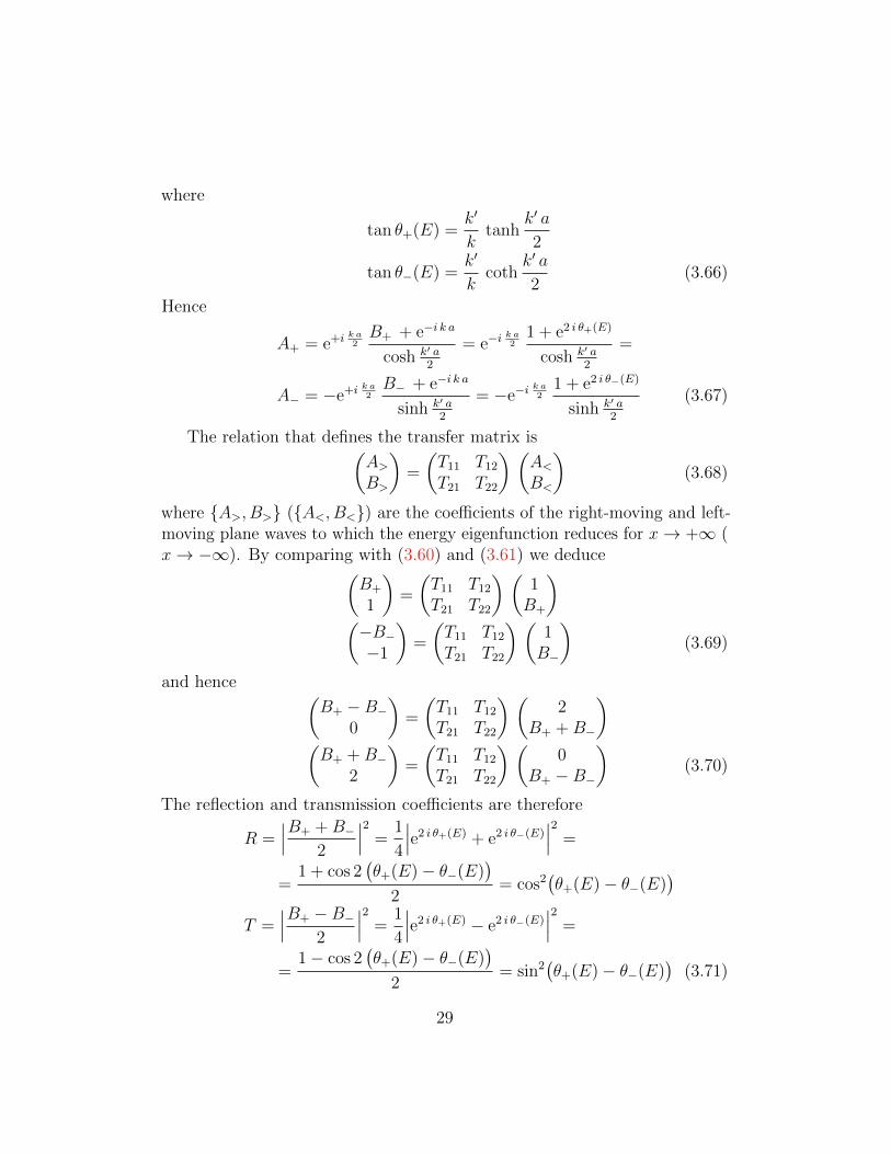
where

tan θ+(E) =k′

ktanh

k′ a

2

tan θ−(E) =k′

kcoth

k′ a

2(3.66)

Hence

A+ = e+i k a2B+ + e−i k a

cosh k′ a2

= e−ik a2

1 + e2 i θ+(E)

cosh k′ a2

=

A− = −e+i k a2B− + e−i k a

sinh k′ a2

= −e−ik a2

1 + e2 i θ−(E)

sinh k′ a2

(3.67)

The relation that defines the transfer matrix is(A>B>

)=

(T11 T12

T21 T22

) (A<B<

)(3.68)

where {A>, B>} ({A<, B<}) are the coefficients of the right-moving and left-moving plane waves to which the energy eigenfunction reduces for x→ +∞ (x→ −∞). By comparing with (3.60) and (3.61) we deduce(

B+

1

)=

(T11 T12

T21 T22

) (1B+

)(−B−−1

)=

(T11 T12

T21 T22

) (1B−

)(3.69)

and hence (B+ −B−

0

)=

(T11 T12

T21 T22

) (2

B+ +B−

)(B+ +B−

2

)=

(T11 T12

T21 T22

) (0

B+ −B−

)(3.70)

The reflection and transmission coefficients are therefore

R =∣∣∣B+ +B−

2

∣∣∣2 =1

4

∣∣∣e2 i θ+(E) + e2 i θ−(E)∣∣∣2 =

=1 + cos 2

(θ+(E)− θ−(E)

)2

= cos2(θ+(E)− θ−(E)

)T =

∣∣∣B+ −B−2

∣∣∣2 =1

4

∣∣∣e2 i θ+(E) − e2 i θ−(E)∣∣∣2 =

=1− cos 2

(θ+(E)− θ−(E)

)2

= sin2(θ+(E)− θ−(E)

)(3.71)

29

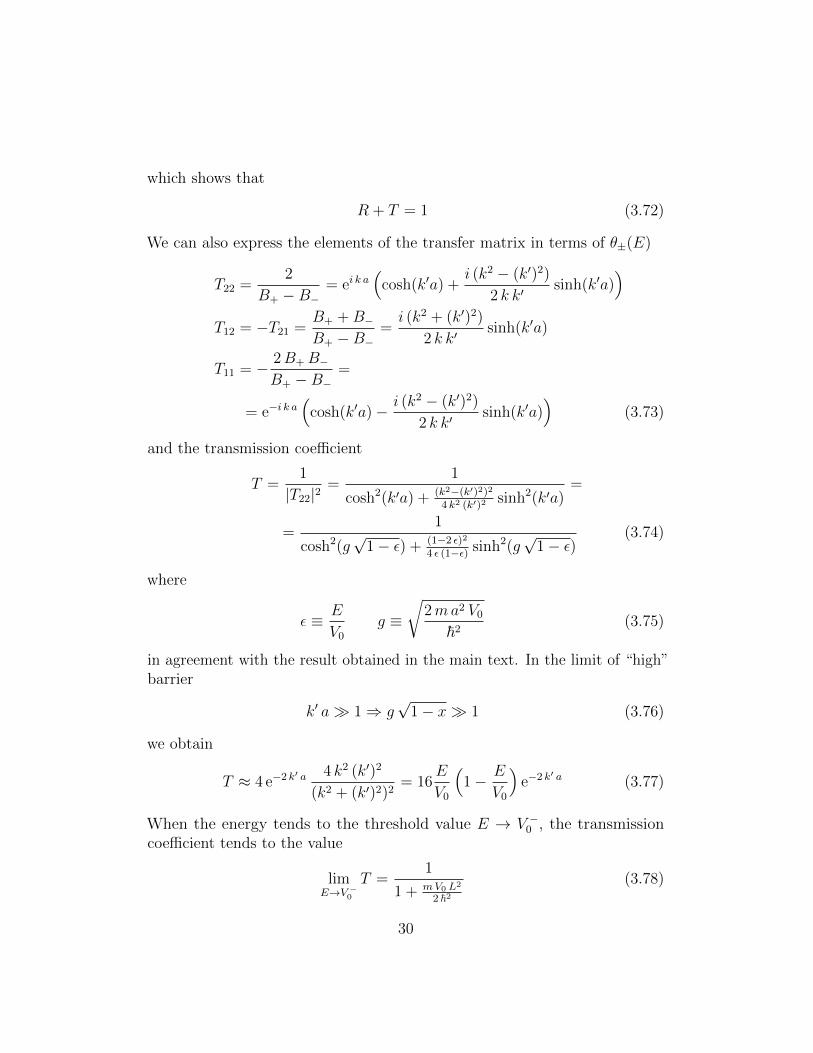
which shows that

R + T = 1 (3.72)

We can also express the elements of the transfer matrix in terms of θ±(E)

T22 =2

B+ −B−= ei k a

(cosh(k′a) +

i (k2 − (k′)2)

2 k k′sinh(k′a)

)T12 = −T21 =

B+ +B−B+ −B−

=i (k2 + (k′)2)

2 k k′sinh(k′a)

T11 = − 2B+ B−B+ −B−

=

= e−i k a(

cosh(k′a)− i (k2 − (k′)2)

2 k k′sinh(k′a)

)(3.73)

and the transmission coefficient

T =1

|T22|2=

1

cosh2(k′a) + (k2−(k′)2)2

4 k2 (k′)2 sinh2(k′a)=

=1

cosh2(g√

1− ε) + (1−2 ε)2

4 ε (1−ε) sinh2(g√

1− ε)(3.74)

where

ε ≡ E

V0

g ≡√

2ma2 V0

~2(3.75)

in agreement with the result obtained in the main text. In the limit of “high”barrier

k′ a� 1⇒ g√

1− x� 1 (3.76)

we obtain

T ≈ 4 e−2 k′ a 4 k2 (k′)2

(k2 + (k′)2)2= 16

E

V0

(1− E

V0

)e−2 k′ a (3.77)

When the energy tends to the threshold value E → V −0 , the transmissioncoefficient tends to the value

limE→V −0

T =1

1 + mV0 L2

2 ~2

(3.78)

30

For E > V0 we derive analogously

T =1

cos2(|k′|a) + (k2+|k′|2)2

4 k2 |k′|2 sin2(|k′|a)=

=1

cos2(g√ε− 1) + (1−2 ε)2

4 ε (ε−1)sin2(g

√ε− 1)

(3.79)

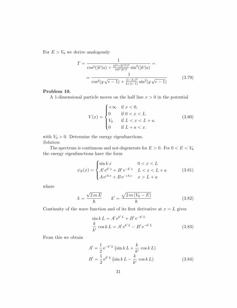
Problem 10.A 1-dimensional particle moves on the half line x > 0 in the potential

V (x) =

+∞ if x < 0,

0 if 0 < x < L.

V0 if L < x < L+ a.

0 if L+ a < x.

(3.80)

with V0 > 0. Determine the energy eigenfunctions.Solution:

The spectrum is continuous and not-degenerate for E > 0. For 0 < E < V0

the energy eigenfunctions have the form

ψE(x) =

sin k x 0 < x < L

A′ ek′ x +B′ e−k

′ x L < x < L+ a

A ei k x +B e−i k x x > L+ a

(3.81)

where

k =

√2mE

~k′ =

√2m (V0 − E)

~(3.82)

Continuity of the wave function and of its first derivative at x = L gives

sin k L = A′ ek′ L +B′ e−k

′ L

k

k′cos k L = A′ ek

′ L −B′ e−k′ L (3.83)

From this we obtain

A′ =1

2e−k

′ L(sin k L+

k

k′cos k L)

B′ =1

2ek′ L(sin k L− k

k′cos k L) (3.84)

31

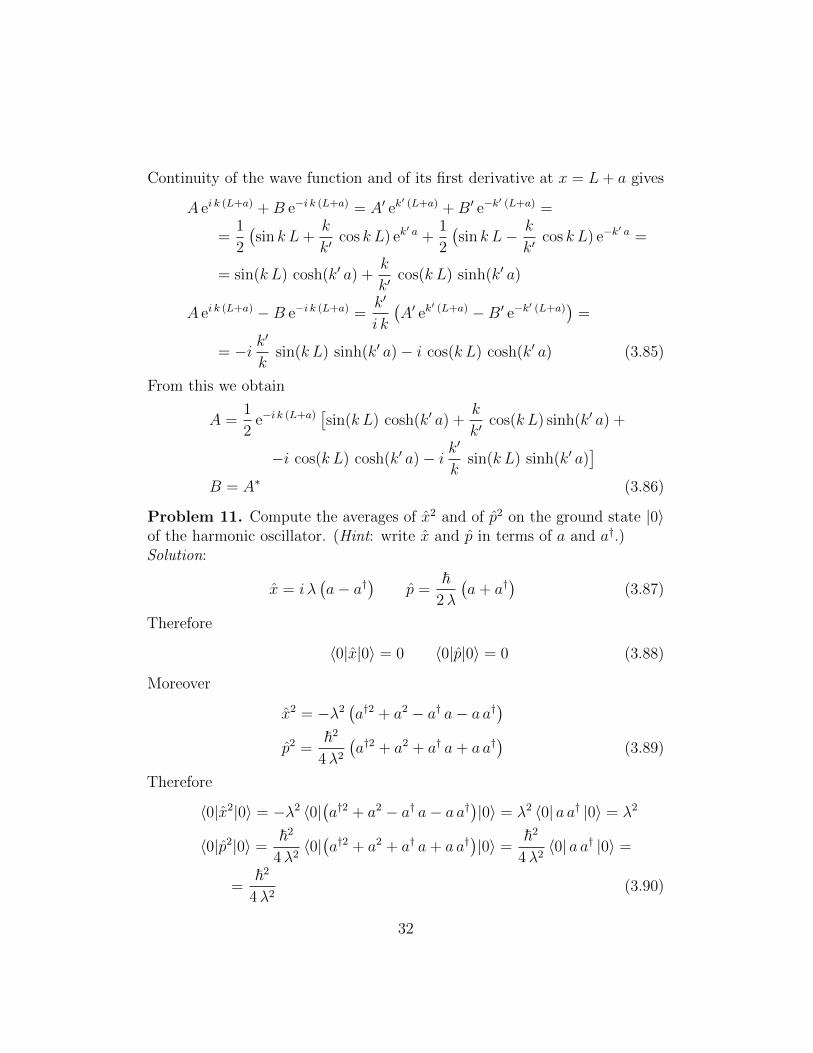
Continuity of the wave function and of its first derivative at x = L+ a gives

A ei k (L+a) +B e−i k (L+a) = A′ ek′ (L+a) +B′ e−k

′ (L+a) =

=1

2

(sin k L+

k

k′cos k L) ek

′ a +1

2

(sin k L− k

k′cos k L) e−k

′ a =

= sin(k L) cosh(k′ a) +k

k′cos(k L) sinh(k′ a)

A ei k (L+a) −B e−i k (L+a) =k′

i k

(A′ ek

′ (L+a) −B′ e−k′ (L+a))

=

= −i k′

ksin(k L) sinh(k′ a)− i cos(k L) cosh(k′ a) (3.85)

From this we obtain

A =1

2e−i k (L+a)

[sin(k L) cosh(k′ a) +

k

k′cos(k L) sinh(k′ a) +

−i cos(k L) cosh(k′ a)− i k′

ksin(k L) sinh(k′ a)

]B = A∗ (3.86)

Problem 11. Compute the averages of x2 and of p2 on the ground state |0〉of the harmonic oscillator. (Hint: write x and p in terms of a and a†.)Solution:

x = i λ(a− a†

)p =

~2λ

(a+ a†

)(3.87)

Therefore

〈0|x|0〉 = 0 〈0|p|0〉 = 0 (3.88)

Moreover

x2 = −λ2(a†2 + a2 − a† a− a a†

)p2 =

~2

4λ2

(a†2 + a2 + a† a+ a a†

)(3.89)

Therefore

〈0|x2|0〉 = −λ2 〈0|(a†2 + a2 − a† a− a a†

)|0〉 = λ2 〈0| a a† |0〉 = λ2

〈0|p2|0〉 =~2

4λ2〈0|(a†2 + a2 + a† a+ a a†

)|0〉 =

~2

4λ2〈0| a a† |0〉 =

=~2

4λ2(3.90)

32

In conclusion

∆x2 = 〈0|x2|0〉 −(〈0|x|0〉

)2= λ2

∆p2 = 〈0|p2|0〉 −(〈0|p|0〉

)2=

~2

4λ2(3.91)

and thus

∆x∆p =~2

(3.92)

The ground state is therefore a state of minimal uncertainty.Problem 12. Consider the state ψ of an harmonic oscillator of frequency ωand mass m which satisfies the equation

aψ = αψ (3.93)

where α is a complex number.a) Find the normalized wave function of ψ in the Schrodinger representa-

tion.b) Compute ∆x and ∆p on the state ψ and show it is a state of minimal

indeterminacy.c) Consider the state

ψ =∞∑n=0

αn√n!|n〉 (3.94)

where |n〉 with n = 0, 1, 2, . . . are the normalized eigenstates of the harmonicoscillator Hamiltonian. Show that ψ satisfies (3.93).

d) Compute the norm of ψ.e) Let ψ be a normalized vector corresponding to ψ. By comparing the

wave function in the Schrodinger representation of ψ with the normalizedwave-function computed in a), derive an explicit formula for the Hermitepolynomials for any n.Solution:a) The wave-function ψ(x) satisfies the differential equation

−i ~ψ′(x)− imω xψ(x) =~αλψ(x) (3.95)

33

that is

ψ′(x)

ψ(x)=i α

λ− x

2λ2(3.96)

The solution is

ψ(x) = C ei αxλ− x2

4λ2 (3.97)

The normalized wave-function is obtained by imposing

1 = 〈ψ, ψ〉 = |C|2∫ ∞−∞

dx ei (α−α) xλ− x2

2λ2 = |C|2 λ∫ ∞−∞

dy ei (α−α) y− y2

2 =

= |C|2 λ√

2π e−(α−α)2

2 (3.98)

Hence

ψ(x) =1

(2π)14

1

λ12

e(α−α)2

4 ei αxλ− x2

4λ2 (3.99)

b) Let us compute ∆x by making use of the Schrodinger representation:

〈ψ, x ψ〉 = |C|2∫ ∞−∞

dx x ei (α−α) xλ− x2

2λ2 = |C|2 λ2

∫ ∞−∞

dy y ei (α−α) y− y2

2 =

= −i |C|2 λ2√

2 π∂

∂(α− α)e−

(α−α)2

2 =

= i |C|2 λ2√

2π (α− α) e−(α−α)2

2 = i (α− α)λ (3.100)

and

〈ψ, x2 ψ〉 = |C|2∫ ∞−∞

dx x2ei (α−α) xλ− x2

2λ2 = |C|2 λ3

∫ ∞−∞

dy y2 ei (α−α) y− y2

2 =

= −|C|2 λ3√

2 π∂2

∂(α− α)2e−

(α−α)2

2 =

= |C|2 λ3√

2π(1− (α− α)2

)e−

(α−α)2

2 = λ2(1− (α− α)2

)(3.101)

Thus

∆x2 = λ2[1− (α− α)2 + (α− α)2

]= λ2 (3.102)

34

For ∆p, let us show how to perform the computation by using raising andlowering operators together with Eq. (3.93). As a matter of fact, this methodis simpler:

〈ψ, p ψ〉 =~

2λ〈ψ, (a+ a†)ψ〉 =

~2λ〈ψ, (α + a†)ψ〉 =

=~

2λ(α + 〈aψ, ψ〉) =

~2λ

(α + α) (3.103)

And

〈ψ, p2 ψ〉 =~2

4λ2〈(a+ a†)ψ, (a+ a†)ψ〉 =

=~2

4λ2

[|α|2 + 〈a† ψ, a† ψ〉+ α2 + α2

]=

=~2

4λ2

[|α|2 + |α|2 + 1 + α2 + α2

]=

=~2

4λ2

[2 |α|2 + 1 + α2 + α2

](3.104)

Hence

∆p2 =~2

4λ2

[2 |α|2 + 1 + α2 + α2 − α2 − α2 − 2 |α|2

]=

~2

4λ2(3.105)

We verified that the state is indeed a state of minimal indeterminacy

∆x∆p =~2

(3.106)

c)

a ψ =∞∑n=1

αn√n!

√n |n− 1〉 =

∞∑n=0

αn+1√(n+ 1)!

√n+ 1 |n〉 =

= α

∞∑n=0

αn√n!|n〉 = α ψ (3.107)

d)

〈ψ, ψ〉 =∞∑n=0

αn√n!

αn√n!

=∞∑n=0

|α|2n

n!= e|α|

2

(3.108)

35

e) From d) we deduce that the vector

ψ = e−|α|2

2 ψ = e−|α|2

2

∞∑n=0

αn√n!|n〉 (3.109)

has unit norm. The wave function of ψ in the Schrodinger representation is

ψ(x) = e−|α|2

2

∞∑n=0

αn√n!ψn(x) = e−

|α|22

∞∑n=0

αn√n!

Hn(xλ)

(2 π)14 λ

12

e−x2

4λ2 (3.110)

Here the ψn(x) are the wave-functions of the energy eigenstates of the harmonicoscillator and the polynomials Hn(y) are defined according to

ψn(x) = 〈x|n〉 =Hn(x

λ)

(2 π)14 λ

12

e−x2

4λ2 (3.111)

Hn(y) are polynomial of degree n, of parity (−1)n, which are (simply relatedto) the so-called Hermite polynomials. In the following we will derive a closedexpression for Hn(x) by comparing Eq. (3.110) with the result obtained in a).

Both ψ(x) and ψ(x) satisfy the equation (3.93) and they both have unitnorm: hence, they can differ at most by a x-independent factor of unit norm

ψ(x) = ei φ(α,α) ψ(x) (3.112)

where φ(α, α) is a real-valued function of α and α. It must therefore be that

1

(2 π)14 λ

12

e−|α|2

2

∞∑n=0

αn√n!Hn(

x

λ) e−

x2

4λ2 =ei φ(α,α)

(2 π)14 λ

12

e(α−α)2

4 ei αxλ− x2

4λ2 (3.113)

or, dividing by the common factors,

∞∑n=0

αn√n!Hn(y) = ei φ(α,α) e

α2

4+ α2

4 ei α y (3.114)

where y ≡ xλ. The LHS of this equation depends only on α. This means that

the factor ei φ(α,α) must cancel the dependence on α of the RHS. In otherwords the combination

ei φ(α,α) eα2

4 = F (α) (3.115)

36

must depend on α but not on α. Since i φ(α, α) is pure imaginary, we concludethat

ei φ(α,α) = e−α2

4+α2

4+i c (3.116)

where c is a real constant independent of both α and α. Then

∞∑n=0

αn√n!Hn(y) = ei c e

α2

2 ei α y (3.117)

The value of the real constant c is determined by taking α→ 0 in both sidesof this equation. In this limit the LHS reduces to H0(y) = 1 and thus

c = 0 (3.118)

We established therefore the identity

∞∑n=0

αn√n!Hn(y) = e

α2

2 ei α y (3.119)

By expanding the RHS in powers of α, and by equating terms with the samepower of α, we obtain the following formula for Hn(x)1

Hn(y) = in[n2

]∑k=0

√n!

2k k!

(−1)k

(n− 2 k)!yn−2 k (3.120)

4 Time evolution

Problem 1. Let E+ and E− the two energy eigenvalues of a 2-states systemand |+〉 and |−〉 the two corresponding energy eigenstates. Suppose that at

1The polynomials Hn(y) defined in (3.111) are related to the Hermite polynomials hn(y)by the formula

Hn(y) =in√n! 2n

hn

( y√2

)The factors in stems from the fact that our definition for a† differs by a factor i from theconventional one. The factor 1√

n! 2nis a factor which is included in the usual definition of

the harmonic oscillator energy eigenfunctions (3.111).

37

the time t = 0 the system is in the state ψ(0) = 1√2

(|+〉+ |−〉

). What is the

probability that at the time t > 0 the system is in the state |+〉?Solution: The state ψ(t) at the time t is

ψ(t) = e−i~ t H ψ(0) = e−

i~ t H

1√2

(|+〉+ |−〉

)=

=1√2

(e−

i~ t E+ |+〉+ e−

i~ t E− |−〉

)(4.121)

The probability that at the time t the system is in the state |+〉 is

P+(t) =∣∣〈+|ψ(t)〉

∣∣2 =∣∣e− i

~ E+ t

√2

∣∣2 =1

2(4.122)

The probability that at the time t the system is in the state ψ(0) is:

Pψ(0)(t) =∣∣〈ψ(0), ψ(t)〉

∣∣2 =∣∣e− i

~ E+ t

2+

e−i~ E− t

2

∣∣2 =

=1

4

(1 + 1 + 2 cos

(E+ − E−) t

~)

=1

2

(1 + cos

(E+ − E−) t

~)

=

= cos2 (E+ − E−) t

2 ~(4.123)

Problem 2An harmonic oscillator of frequency ω is, at time t = 0, in the state

ψ0 = |0〉+ |1〉+ |2〉 (4.124)

• a) Compute the average of p and p2 at the time t.

• b) Write the normalized wave function of the state at the time t in theSchrodinger representation.

• c) What is the probability that at the time t > 0 the system is still inthe state ψ0?

Solution: The state at the time t is

ψ(t) = e−iω t2

[|0〉+ e−i ω t |1〉+ e−2 i ω t |2〉

](4.125)

38

• a) Therefore

〈ψ(t), p ψ(t)〉 =~

2λ〈ψ(t),

(a+ a†

)ψ(t)〉 =

= e−iω t2

~2λ〈ψ(t),

[e−i ω t |0〉+ e−2 i ω t

√2 |1〉+

+|1〉+ e−i ω t√

2 |2〉+ e−2 i ω t√

3 |3〉]〉 =

=~

2λ

[e−i ω t + e−i ω t

√2 + ei ω t + ei ω t

√2]

=

=~λ

(1 +√

2) cos(ω t) (4.126)

The average of p is therefore

p(t) =〈ψ(t), p ψ(t)〉〈ψ(t), ψ(t)〉

=~

3λ(1 +

√2) cos(ω t) (4.127)

• b) Moreover

〈ψ(t), p2 ψ(t)〉 = 〈p ψ(t), p ψ(t)〉 =

=~2

4λ2

∣∣∣e−i ω t |0〉+ (1 +√

2 e−2 i ω t) |1〉+

+e−i ω t√

2 |2〉+ e−2 i ω t√

3 |3〉∣∣∣2 =

=~2

4λ2

(1 + |1 +

√2 e−2 i ω t|2 + 2 + 3

)=

=~2

4λ2

(6 + (3 + 2

√2 cos(2ω t))

)=

=~2

4λ2

(9 + 2

√2 cos(2ω t)

)(4.128)

The average of p2 is therefore

p2(t) =1

3〈ψ(t), p2 ψ(t)〉 =

~2

12λ2

(9 + 2

√2 cos(2ω t)

)(4.129)

• c) The probability that at the time t > 0 the system is still in the state

39

ψ0 is

Pψ0→ψ0(t) =1

9

∣∣〈ψ0, ψ(t)〉∣∣2 =

1

9

∣∣∣〈|0〉+ |1〉+ |2〉,

|0〉+ e−i ω t |1〉+ e−2 i ω t |2〉〉∣∣∣2 =

1

9

∣∣∣1 + e−i ω t + e−2 i ω t∣∣∣2 =

=1

9

(3 + 4 cos(ω t) + 2 cos(2ω t)

)(4.130)

Problem 4. Determine the time evolution of the free wave packet

vp,∆p(x) =1

(π)14 ∆

12p

∫dp e

− (p−p)2

2 ∆2p

ei~ p x

√2π ~

(4.131)

Solution: The wave function at the time t is

vp,∆p(x; t) = e−i~ H t vp,∆p(x) =

1

(π)14 ∆

12p

∫dp e

− (p−p)2

2 ∆2p

ei~ p x−

i~p2

2mt

√2π ~

=

=ei~ p x−

i~p2 t2m

(π)14

√2 π ~∆

12p

∫dp e

−(1+i t∆2p

m ~ ) p2

2 ∆2p

+ i~ p (x− p

mt)

=

=ei~ p x−

i~p2 t2m

(π)14

√2 π ~∆

12p

√2 π∆p√

i~

∆2p

mt+ 1

e−

∆2p (x− p

m t)2

2 ~2 (1+i t∆2p

~m ) =

=ei~ p x−

i~p2 t2m

~ 12 (π)

14

∆12p√

i∆2p

m ~ t+ 1e−

∆2p (x− p

m t)2

2 ~2 (1+i t∆2p

~m ) (4.132)

Problem 5. Compute the uncertainties of x and p on the free wave packet(4.131) for t > 0. (Hint: Use the Heisenberg picture of time evolution.)Solution: Since the particle is free, the time dependent operators x(t) andp(t) in the Heisenberg picture are

x(t) = x+p

mt p(t) = p(0) = p (4.133)

Therefore

x2(t) = x2 +p2

m2t2 +

t

m(x p+ p x)

p2(t) = p2(0) = p2 (4.134)

40

Denote by |v〉 the state described by the wave function (4.131):

vp,∆p(x) =

√∆p

(π)14

√~

e−∆2p x

2

2 ~2 ei~ p x (4.135)

Then

〈v|x2(t) |v〉 = 〈v|x2|v〉+t2

m2〈v|p2|v〉+

t

m〈v|(x p+ p x) |v〉(

〈v|x(t) |v〉)2

=(〈v|x|v〉+

t

m〈v|p|v〉

)2=

= 〈v|x|v〉2 +t2

m2〈v|p|v〉2 + 2

t

m〈v|p|v〉 〈v|x|v〉

=t2

m2p2

〈v|p2(t) |v〉 = 〈v|p2|v〉〈v|p |v〉2 = p2 (4.136)

since

〈v|p|v〉 = p 〈v|x|v〉 = 0 (4.137)

The uncertainties on x and p at the time t are therefore

∆x2(t) = ∆x2 +t2

m2∆p2 +

2 t

m〈v|x p|v〉 − i ~ t

m∆p2(t) = ∆p2 (4.138)

We are left with the computation of the matrix element

〈v|x p|v〉 =∆p√π ~

∫dx e−

∆2p x

2

~2(x p+ i x2

∆2p

~)

=

=∆p√π ~

i∆2p

~

∫dx e−

∆2p x

2

~2 x2 =i∆3

p√π ~2

√π ~3

2 ∆3p

=

=i ~2

(4.139)

In conclusion

∆x(t) =

√∆x2 +

t2

m2∆p2

∆p(t) = ∆p (4.140)

41

Problem 6. Estimate the speed at which the following free wave packets, ofminimal indeterminacy at t = 0, spread for large t:

• An electron with ∆x ≈ 10−8 cm.

• An electron with ∆x ≈ 10−2 cm.

• A grain of sand of m = 10−12g, with ∆x = 10−5cm.

Solution: The speed at which the packets of minimal indeterminacy spread is,according to the solution of the previous problem, is for large t

d∆x(t)

dt≈ ~

2m∆x(4.141)

Recall that the electron Compton wavelength is

λc =~mc

= 0.387× 10−12m (4.142)

Therefore for an electron

d∆x(t)

dt≈ λc

∆xc (4.143)

For ∆x = 10−8 cm = 10−10m

d∆x(t)

dt≈ 1

2× 0.387× 10−2 × 3× 108m/s = 0.580× 106m/s (4.144)

For ∆x = 10−2 cm = 10−4m

d∆x(t)

dt≈ 1

2× 0.387× 10−8 × 3× 108m/s = 0.580m/s (4.145)

For a grain of sand of mass

m = 10−12g = 10−15 kg = 1.10× 1015melectron (4.146)

and ∆x = 10−5cm = 10−7m, we have

d∆x(t)

dt≈ 1

2× 0.387× 10−5

1.10× 1015× 3× 108m/s = 0.527× 10−12m/s (4.147)

“Large” time t means

t� m∆x

∆p=m∆x2

~=

∆x~

m∆x

(4.148)

that is

t~

m∆x� ∆x (4.149)

42

5 Symmetries

Problem 4. A spin 1 system is in the state with Sz = +1. Find theprobabilities that the measurement of Sx gives the values Sx = −1, 0, 1.Solution.

Let {|Sz〉, Sz = −1, 0, 1} of eigenstates of Sz be the states of eigenstatesof Sz. Let us determine the matrix which represents Sx in such a basis. Wehave

Sx =S+ + S−

2Sy =

S+ − S−2 i

(5.1)

and

S+|1〉 = 0 S+|0〉 =√

2 |1〉 S+| − 1〉 =√

2 |0〉S−|1〉 =

√2 |0〉 S−|0〉 =

√2 | − 1〉 S−| − 1〉 = 0 (5.2)

Therefore

Sx|1〉 =1√2|0〉 Sx|0〉 =

1√2

(|1〉+ | − 1〉

)Sx | − 1〉 =

1√2|0〉

The matrix which represents Sx in the {|1〉, |0〉, | − 1〉} basis is therefore

Sx =

0 1√2

01√2

0 1√2

0 1√2

0

(5.3)

The eigenvalues of this matrix are given by the equation

0 = det

−mx1√2

01√2−mx

1√2

0 1√2−mx

= −mx (m2x −

1

2)− 1√

2(−mx√

2) =

= mx (1−m2x) (5.4)

and are, as expected, mx = 1, 0,−1. The eigenstate (x, y, z) corresponding tothe eigenvalue mx satisfies

−mx x+y√2

= 0

x√2−mx y +

z√2

= 0

y√2−mx z = 0 (5.5)

43

For mx = 1 this gives

x = z =y√2

(5.6)

Therefore the normalized eigenstate with mx = 1 is

|Sx = 1〉 =

121√2

12

(5.7)

When mx = 0 we have

y = 0 x = −z (5.8)

from which one derives the normalized eigenstate with mx = 0

|Sx = 0〉 =

1√2

0− 1√

2

(5.9)

Finally, Eqs. (5.5) for mx = −1 become

x = z = − y√2

(5.10)

from which

|Sx = −1〉 =

12

− 1√2

12

(5.11)

These equations rewrite in a representation independent form as follows

|Sx = 1〉 =1

2|1〉+

1√2|0〉+

1

2| − 1〉

|Sx = 0〉 =1√2|1〉 − 1√

2| − 1〉

|Sx = −1〉 =1

2|1〉 − 1√

2|0〉+

1

2| − 1〉 (5.12)

44

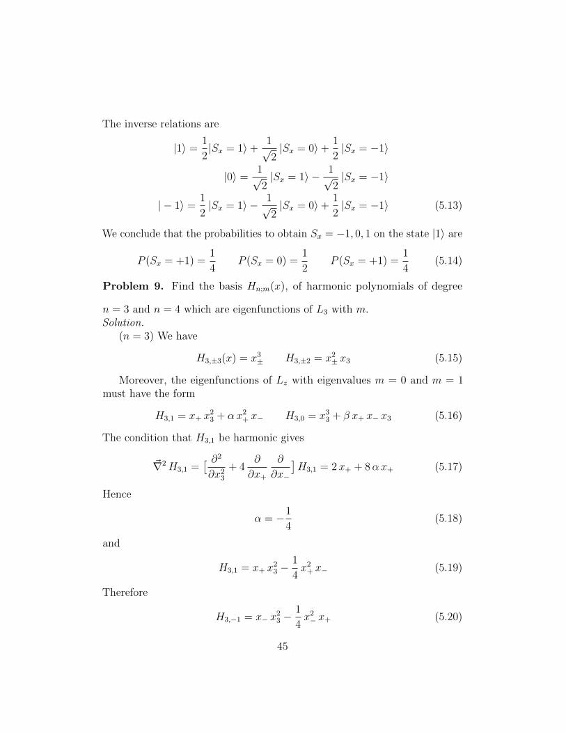
The inverse relations are

|1〉 =1

2|Sx = 1〉+

1√2|Sx = 0〉+

1

2|Sx = −1〉

|0〉 =1√2|Sx = 1〉 − 1√

2|Sx = −1〉

| − 1〉 =1

2|Sx = 1〉 − 1√

2|Sx = 0〉+

1

2|Sx = −1〉 (5.13)

We conclude that the probabilities to obtain Sx = −1, 0, 1 on the state |1〉 are

P (Sx = +1) =1

4P (Sx = 0) =

1

2P (Sx = +1) =

1

4(5.14)

Problem 9. Find the basis Hn;m(x), of harmonic polynomials of degree

n = 3 and n = 4 which are eigenfunctions of L3 with m.Solution.

(n = 3) We have

H3,±3(x) = x3± H3,±2 = x2

± x3 (5.15)

Moreover, the eigenfunctions of Lz with eigenvalues m = 0 and m = 1must have the form

H3,1 = x+ x23 + αx2

+ x− H3,0 = x33 + β x+ x− x3 (5.16)

The condition that H3,1 be harmonic gives

~∇2H3,1 =[ ∂2

∂x23

+ 4∂

∂x+

∂

∂x−

]H3,1 = 2x+ + 8αx+ (5.17)

Hence

α = −1

4(5.18)

and

H3,1 = x+ x23 −

1

4x2

+ x− (5.19)

Therefore

H3,−1 = x− x23 −

1

4x2− x+ (5.20)

45

Analogously

~∇2H3,0 = (6 + 4 β)x3 (5.21)

Hence

β = −3

2(5.22)

and

H3,0 = x33 −

3

2x+ x− x3 (5.23)

Problem 10.Consider a 3-dimensional particle of mass m moving in a harmonic poten-

tial

V (r) =1

2mω2 r2 (5.24)

Show that:

• a) The energy levels are given by En = ~ (n+ 32) with n = 0, 1, 2, . . ..

• b) The ground state is non-degenerate and has l = 0. Find the normal-ized radial wave function χE0,0(r) with l = 0.

• c) The first excited level E1 has degeneracy 3 and l = 1. Find thenormalized radial wave function χE1,1(r) with l = 1.

(Hint: Since one can write the 3-dimensional hamiltonian H =∑3

i=1 Hi

where Hi =p2i

2m+ 1

2mω2 x2

i is the hamiltonian of the 1-dimensional harmonicoscillator, the energy eigenfunctions of the 3-dimensional oscillator are

ψn1,n2,n3(~x) = ψn1(x1)ψn2(x2)ψn3(x3) (5.25)

where ψni(xi) are the eigenfunctions of the 1-dimensional harmonic oscillators.)Solution.

a) The energy levels corresponding to the wave functions

ψn1,n2,n3(~x) = ψn1(x1)ψn2(x2)ψn3(x3) (5.26)

46

are

En1,n2,n3 =3∑i=1

~ω (ni +1

2) = ~ω(n+

3

2) (5.27)

where

n ≡ n1 + n2 + n3 (5.28)

b) The ground state corresponds to

n = 0 = n1 = n2 = n3 (5.29)

It is non-degenerate and has wave function

ψ0,0,0(~x) = ψ0(x1)ψ0(x2)ψ0(x3) =3∏i=1

(mω

π ~

) 14

e−mω2 ~ x2

i =

=(mω

π ~

) 34

e−mω2 ~ r2

(5.30)

Since this level is non-degenerate, it necessarily has l = 0 and m = 0:

ψ0,0,0(~x) = Y0,0(θ, φ)RE0,0(r) (5.31)

Therefore the radial wave function is

χE0,0(r) = r RE0,0(r) =√

4π(mω

π ~

) 34r e−

mω2 ~ r2

=2

π14

(mω

~

) 34r e−

mω2 ~ r2

(5.32)

c) The first excited level has n = 1 and therefore it corresponds to thethree degenerate normalized wave functions

ψ1,0,0(~x) =

√2mω

~x1

(mω

π ~

) 34

e−mω2 ~ r2

ψ0,1,0(~x) =

√2mω

~x2

(mω

π ~

) 34

e−mω2 ~ r2

ψ0,0,1(~x) =

√2mω

~x3

(mω

π ~

) 34

e−mω2 ~ r2

(5.33)

47

The wave function ψ0,0,1 can re-written as

ψ0,0,1(~x) =

√8 π

3Y1,0(θ, φ)

(mω

~

) 12r(mω

π ~

) 34

e−mω2 ~ r2

=

= Y1,0(θ, φ)RE1,1(r) (5.34)

where

RE1,1(r) =

√8

3

r

π14

(mω

~

) 54

e−mω2 ~ r2

(5.35)

Hence this is a state with l = 1 and m = 0 and the associated radial wavefunction is

χE1,1(r) = r RE1,1(r) =1

π14

√8

3r2(mω

π ~

) 54

e−mω2 ~ r2

(5.36)

The following linear combinations of the ψ1,0,0 and ψ0,1,0 are the wave functionsof the states with l = 1 and m = ±1

1√2

(ψ1,0,0(~x)± i ψ0,1,0(~x)

)=

(x1 ± i x2)

π34

(mω

~

) 54

e−mω2 ~ r2

=

= ± i Y1,±1(θ, φ)

√8

3

r

π14

(mω

~

) 54

e−mω2 ~ r2

=

= ±i Y1,±1(θ, φ)RE1,1(r) (5.37)

Problem 11.Show that the radial wave function of the ground state of the hydrogenoid

χE,0(r) = 2( ZaB

) 32r e−Z raB (5.38)

has norm one.Solution.

∫ ∞0

dr |χE,0(r)|2 = 4( ZaB

)3∫ ∞

0

dr r2 e− 2Z r

aB =

=1

2

∫ ∞0

dρ ρ2 e−ρ = 1 (5.39)

48

Problem 12. Find the normalized radial wave function of the first excitedstate with l = 0 of the hydrogenoid atom by looking for solutions of

χE,0(ρ) = ρ(b0 + b1 ρ

)e−c ρ c > 0 (5.40)

Solution. We have

χ′E,0(ρ) =[b0 + 2 b1 ρ− cρ

(b0 + b1 ρ

)]e−c ρ =

=[b0 + (2 b1 − c b0) ρ− c b1 ρ

2]

e−c ρ

χ′′E,0(ρ) =[(2 b1 − c b0) − 2 c b1 ρ− c b0 +

−c (2 b1 − c b0) ρ+ c2 b1 ρ2]

e−c ρ =

=[(2 b1 − 2 c b0) + (c2 b0 − 4 c b1) ρ+ c2 b1 ρ

2]

e−c ρ (5.41)

Therefore

χ′′E,0(ρ)

χE,0(ρ)=

(2 b1 − 2 c b0) + (c2 b0 − 4 c b1) ρ+ c2 b1 ρ2

ρ(b0 + b1 ρ

) =

= − E

Z2 |EH1 |− 2

ρ(5.42)

Equivalently

(2 b1 − 2 c b0) + (c2 b0 − 4 c b1) ρ+ c2 b1 ρ2 =

= −(ρ

E

Z2 |EH1 |

+ 2) (b0 + b1 ρ

)=

= −2 b0 −(2 b1 + b0

E

Z2 |EH1 |)ρ− ρ2 E

Z2 |EH1 |

b1 (5.43)

From this we obtain the equations

2 b1 − 2 c b0 = −2 b0

−c2 b0 + 4 c b1 = 2 b1 + b0E

Z2 |EH1 |

c2 b1 = − E

Z2 |EH1 |

b1 (5.44)

49

From the third equation we obtain

c2 = − E

Z2 |EH1 |

(5.45)

Replacing this in the second equation we conclude

(4 c− 2) b1 = 0 (5.46)

If c 6= 12, this would give b1 = 0. Replacing this value in the first equation we

would obtain

(c− 1) b0 = 0 (5.47)

Since b0 6= 0 (otherwise we would recover the trivial solution b0 = b1 = 0),then c = 1. But this is the ground state solution ∝ e−ρ. The excited statecorresponds to choosing the solution with b1 6= 0, and therefore

c =1

2(5.48)

The first equation gives then

b1 = −1

2b0 (5.49)

In conclusion there is a normalizable solution, whose energy eigenvalue is

E2 =Z2E1

4(5.50)

and whose radial wave function is

χE2,0(ρ) = b0 ρ(1− 1

2ρ)

e−ρ2 (5.51)

This is the |2, 0, 0〉 excited state of the hydrogenoid. The normalization factoris determined by

1 =aBZ

∫ ∞0

dρ∣∣χE2,0(ρ)

∣∣2 =aB |b0|2

Z

∫ ∞0

dρ ρ2(1− 1

2ρ)2

e−ρ =

=2 |b0|2 aB

Z(5.52)

Therefore

b0 =

√Z

2 aB(5.53)

50