an introduction to ordinary differential equations...
TRANSCRIPT


Universitext

Ravi P. Agarwal
Donal O’Regan
An Introduction to Ordinary Differential Equations

Ravi P. AgarwalFlorida Institute of TechnologyDepartment of Mathematical Sciences150 West University Blvd.Melbourne, FL 32901agarwal@fi t.edu
Donal O’ReganNational University of Ireland, GalwayMathematics DepartmentUniversity RoadGalway, [email protected]
ISBN: 978-0-387-71275-8 e-ISBN: 978-0-387-71276-5DOI: 10.1007/978-0-387-71276-5
Library of Congress Control Number: 2007935982
Mathematics Subject Classifi cation (2000): 34-01, 34-XX
©2008 Springer Science+Business Media LLCAll rights reserved. This work may not be translated or copied in whole or in part without the written permission of the publisher (Springer Science+Business Media LLC, 233 Spring Street, New York, NY 10013, U.S.A.), except for brief excerpts in connection with reviews or scholarly analysis. Use in connection with any form of information storage and retrieval, electronic adaptation, computer software, or by similar or dissimilar methodology now known or hereafter developed is forbidden.The use in this publication of trade names, trademarks, service marks and similar terms, even if they are not identifi ed as such, is not to be taken as an expression of opinion as to whether or not they are subject to proprietary rights.
Printed on acid-free paper.
9 8 7 6 5 4 3 2 1
springer.com

Dedicated to
Ramesh C. Guptaon his 65th birthday

Preface
Ordinary differential equations serve as mathematical models for manyexciting “real-world” problems, not only in science and technology, but alsoin such diverse fields as economics, psychology, defense, and demography.Rapid growth in the theory of differential equations and in its applicationsto almost every branch of knowledge has resulted in a continued interest inits study by students in many disciplines. This has given ordinary differen-tial equations a distinct place in mathematics curricula all over the worldand it is now being taught at various levels in almost every institution ofhigher learning.
Hundreds of books on ordinary differential equations are available. How-ever, the majority of these are elementary texts which provide a battery oftechniques for finding explicit solutions. The size of some of these books hasgrown dramatically—to the extent that students are often lost in decidingwhere to start. This is all due to the addition of repetitive examples and ex-ercises, and colorful pictures. The advanced books are either on specializedtopics or are encyclopedic in character. In fact, there are hardly any rigor-ous and perspicuous introductory texts available which can be used directlyin class for students of applied sciences. Thus, in an effort to bring the sub-ject to a wide audience we provide a compact, but thorough, introductionto the subject in An Introduction to Ordinary Differential Equations. Thisbook is intended for readers who have had a course in calculus, and hence itcan be used for a senior undergraduate course. It should also be suitable fora beginning graduate course, because in undergraduate courses, studentsdo not have any exposure to various intricate concepts, perhaps due to aninadequate level of mathematical sophistication.
The subject matter has been organized in the form of theorems andtheir proofs, and the presentation is rather unconventional. It comprises 42class-tested lectures which the first author has given to mostly math-majorstudents at various institutions all over the globe over a period of almost 35years. These lectures provide flexibility in the choice of material for a one-semester course. It is our belief that the content in each lecture, togetherwith the problems therein, provides fairly adequate coverage of the topicunder study.
A brief description of the topics covered in this book is as follows:Introductory Lecture 1 explains basic terms and notations that are usedthroughout the book. Lecture 2 contains a concise account of the historicaldevelopment of the subject. Lecture 3 deals with exact differential equa-tions, while first-order equations are studied in Lectures 4 and 5. Lecture 6discusses second-order linear differential equations; variation of parameters

viii Preface
is used here to find solutions to nonhomogeneous equations. Lectures 3–6form the core of any course on differential equations.
Many very simple differential equations cannot be solved as finite com-binations of elementary functions. It is, therefore, of prime importance toknow whether a given differential equation has a solution. This aspect ofthe existence of solutions for first-order initial value problems is dealt within Lectures 8 and 9. Once the existence of solutions has been established, itis natural to provide conditions under which a given problem has preciselyone solution; this is the content of Lecture 10. In an attempt to make thepresentation self-contained, the required mathematical preliminaries havebeen included in Lecture 7. Differential inequalities, which are importantin the study of qualitative as well as quantitative properties of solutions,are discussed in Lecture 11. Continuity and differentiability of solutionswith respect to initial conditions are examined in Lecture 12.
Preliminary results from algebra and analysis required for the study ofdifferential systems are contained in Lectures 13 and 14. Lectures 15 and16 extend existence–uniqueness results and examine continuous dependenceon initial data for the systems of first-order initial value problems. Basicproperties of solutions of linear differential systems are given in Lecture 17.Lecture 18 deals with the fundamental matrix solution, and some methodsfor its computation in the constant-coefficient case are discussed in Lecture19. These computational algorithms do not use the Jordan form and caneasily be mastered by students. In Lecture 20 necessary and sufficientconditions are provided so that a linear system has only periodic solutions.Lectures 21 and 22 contain restrictions on the known quantities so thatsolutions of a linear system remain bounded or ultimately approach zero.Lectures 23–29 are devoted to a self-contained introductory stability theoryfor autonomous and nonautonomous systems. Here two-dimensional linearsystems form the basis for the phase plane analysis. In addition to thestudy of periodic solutions and limit cycles, the direct method of Lyapunovis developed and illustrated.
Higher-order exact and adjoint equations are introduced in Lecture 30,and the oscillatory behavior of solutions of second-order equations is fea-tured in Lecture 31.
The last major topic covered in this book is that of boundary value prob-lems involving second-order differential equations. After linear boundaryvalue problems are introduced in Lecture 32, Green’s function and its con-struction is discussed in Lecture 33. Lecture 34 describes conditions thatguarantee the existence of solutions of degenerate boundary value prob-lems. The concept of the generalized Green’s function is also featuredhere. Lecture 35 presents some maximum principles for second-order lin-ear differential inequalities and illustrates their importance in initial and

Preface ix
boundary value problems. Lectures 36 and 37 are devoted to the studyof Sturm–Liouville problems, while eigenfunction expansion is the subjectof Lectures 38 and 39. A detailed discussion of nonlinear boundary valueproblems is contained in Lectures 40 and 41.
Finally, Lecture 42 addresses some topics for further study which extendthe material of this text and are of current research interest.
Two types of problems are included in the book—those which illustratethe general theory, and others designed to fill out text material. The prob-lems form an integral part of the book, and every reader is urged to attemptmost, if not all of them. For the convenience of the reader we have pro-vided answers or hints for all the problems, except those few marked withan asterisk.
In writing a book of this nature no originality can be claimed. Our goalhas been made to present the subject as simply, clearly, and accurately aspossible. Illustrative examples are usually very simple and are aimed at theaverage student.
It is earnestly hoped that An Introduction to Ordinary DifferentialEquations will provide an inquisitive reader with a starting point in thisrich, vast, and ever-expanding field of knowledge.
We would like to express our appreciation to Professors M. Bohner,A. Cabada, M. Cecchi, J. Diblik, L. Erbe, J. Henderson, Wan-Tong Li,Xianyi Li, M. Migda, Ch. G. Philos, S. Stanek, C. C. Tisdell, and P. J. Y.Wong for their suggestions and criticisms. We also want to thank Ms.Vaishali Damle at Springer New York for her support and cooperation.
Ravi P. AgarwalDonal O’Regan

Contents
Preface vii
1. Introduction 1
2. Historical Notes 7
3. Exact Equations 13
4. Elementary First-Order Equations 21
5. First-Order Linear Equations 28
6. Second-Order Linear Equations 35
7. Preliminaries to Existence and Uniqueness of Solutions 45
8. Picard’s Method of Successive Approximations 53
9. Existence Theorems 61
10. Uniqueness Theorems 68
11. Differential Inequalities 77
12. Continuous Dependence on Initial Conditions 84
13. Preliminary Results from Algebra and Analysis 91
14. Preliminary Results from Algebra and Analysis (Contd.) 97
15. Existence and Uniqueness of Solutions of Systems 103
16. Existence and Uniqueness of Solutions of Systems (Contd.) 109
17. General Properties of Linear Systems 116
18. Fundamental Matrix Solution 124
19. Systems with Constant Coefficients 133
20. Periodic Linear Systems 144

xii Contents
21. Asymptotic Behavior of Solutions of Linear Systems 152
22. Asymptotic Behavior of Solutions of Linear Systems (Contd.) 159
23. Preliminaries to Stability of Solutions 168
24. Stability of Quasi-Linear Systems 175
25. Two-Dimensional Autonomous Systems 181
26. Two-Dimensional Autonomous Systems (Contd.) 187
27. Limit Cycles and Periodic Solutions 196
28. Lyapunov’s Direct Method for Autonomous Systems 204
29. Lyapunov’s Direct Method for Nonautonomous Systems 211
30. Higher-Order Exact and Adjoint Equations 217
31. Oscillatory Equations 225
32. Linear Boundary Value Problems 233
33. Green’s Functions 240
34. Degenerate Linear Boundary Value Problems 250
35. Maximum Principles 258
36. Sturm–Liouville Problems 265
37. Sturm–Liouville Problems (Contd.) 271
38. Eigenfunction Expansions 279
39. Eigenfunction Expansions (Contd.) 286
40. Nonlinear Boundary Value Problems 295
41. Nonlinear Boundary Value Problems (Contd.) 300
42. Topics for Further Studies 308
References 315
Index 319

Lecture 1Introduction
An ordinary differential equation (ordinary DE hereafter) is a relationcontaining one real independent variable x ∈ IR = (−∞,∞), the real de-pendent variable y, and some of its derivatives y′, y′′, . . . , y(n) (′= d/dx).For example,
xy′ + 3y = 6x3 (1.1)
y′2 − 4y = 0 (1.2)
x2y′′ − 3xy′ + 3y = 0 (1.3)
2x2y′′ − y′2 = 0. (1.4)
The order of an ordinary DE is defined to be the order of the highestderivative in the equation. Thus, equations (1.1) and (1.2) are first order,whereas (1.3) and (1.4) are second order.
Besides ordinary DEs, if the relation has more than one independentvariable, then it is called a partial DE. In these lectures we shall discussonly ordinary DEs, and so the word ordinary will be dropped.
In general, an nth-order DE can be written as
F (x, y, y′, y′′, . . . , y(n)) = 0, (1.5)
where F is a known function.
A functional relation between the dependent variable y and the inde-pendent variable x, that, in some interval J, satisfies the given DE is saidto be a solution of the equation. A solution may be defined in either ofthe following intervals: (α, β), [α, β), (α, β], [α, β], (α,∞), [α,∞), (−∞,β), (−∞, β], (−∞,∞), where α, β ∈ IR and α < β. For example, thefunction y(x) = 7ex + x2 + 2x + 2 is a solution of the DE y′ = y − x2
in J = IR. Similarly, the function y(x) = x tan(x + 3) is a solution of theDE xy′ = x2 + y2 + y in J = (−π/2 − 3, π/2 − 3). The general solution ofan nth-order DE depends on n arbitrary constants; i.e., the solution y de-pends on x and the real constants c1, c2, . . . , cn. For example, the functiony(x) = x2 +cex is the general solution of the DE y′ = y−x2 +2x in J = IR.Similarly, y(x) = x3 + c/x3, y(x) = x2 + cx+ c2/4, y(x) = c1x+ c2x
3 andy(x) = (2x/c1)− (2/c21) ln(1+c1x)+c2 are the general solutions of the DEs(1.1)–(1.4), respectively. Obviously, the general solution of (1.1) is definedin any interval which does not include the point 0, whereas the general
R.P. Agarwal and D. O’Regan, An Introduction to Ordinary Differential Equations, 1 doi: 10.1007/978-0-387-71276-5_1, © Springer Science + Business Media, LLC 2008

2 Lecture 1
solutions of (1.2) and (1.3) are defined in J = IR. The general solution of(1.4) imposes a restriction on the constant c1 as well as on the variable x.In fact, it is defined if c1 = 0 and 1 + c1x > 0.
The function y(x) = x3 is a particular solution of the equation (1.1),and it can be obtained easily by taking the particular value of c as 0 inthe general solution. Similarly, if c = 0 and c1 = 0, c2 = 1 in the generalsolutions of (1.2) and (1.3), then x2 and x3, respectively, are the particularsolutions of the equations (1.2) and (1.3). It is interesting to note thaty(x) = x2 is a solution of the DE (1.4); however, it is not included in thegeneral solution of (1.4). This “extra” solution, which cannot be obtainedby assigning particular values of the constants, is called a singular solutionof (1.4). As an another example, for the DE y′2 − xy′ + y = 0 the generalsolution is y(x) = cx − c2, which represents a family of straight lines, andy(x) = x2/4 is a singular solution which represents a parabola. Thus, inthe “general solution,” the word general must not be taken in the sense ofcomplete. A totality of all solutions of a DE is called a complete solution.
A DE of the first order may be written as F (x, y, y′) = 0. The functiony = φ(x) is called an explicit solution provided F (x, φ(x), φ′(x)) = 0 in J.
A relation of the form ψ(x, y) = 0 is said to be an implicit solution ofF (x, y, y′) = 0 provided it determines one or more functions y = φ(x) whichsatisfy F (x, φ(x), φ′(x)) ≡ 0. It is frequently difficult, if not impossible, tosolve ψ(x, y) = 0 for y. Nevertheless, we can test the solution by obtainingy′ by implicit differentiation: ψx + ψyy
′ = 0, or y′ = −ψx/ψy, and check ifF (x, y,−ψx/ψy) ≡ 0.
The pair of equations x = x(t), y = y(t) is said to be a parametricsolution of F (x, y, y′) = 0 when F (x(t), y(t), (dy/dt)/(dx/dt)) ≡ 0.
Consider the equation y′′′2 − 2y′y′′′ + 3y′′3 = 0. This is a third-orderDE and we say that this is of degree 2, whereas the second-order DE xy′′ +2y′ + 3y − 6ex = 0 is of degree 1. In general, if a DE has the form of analgebraic equation of degree k in the highest derivative, then we say thatthe given DE is of degree k.
We shall always assume that the DE (1.5) can be solved explicitly fory(n) in terms of the remaining (n+ 1) quantities as
y(n) = f(x, y, y′, . . . , y(n−1)), (1.6)
where f is a known function. This will at least avoid having equation (1.5)represent more than one equation of the form (1.6); e.g., y′2 = 4y representstwo DEs, y′ = ±2
√y.
Differential equations are classified into two groups: linear and nonlin-ear. A DE is said to be linear if it is linear in y and all its derivatives.

Introduction 3
Thus, an nth-order linear DE has the form
Pn[y] = p0(x)y(n) + p1(x)y(n−1) + · · · + pn(x)y = r(x). (1.7)
Obviously, DEs (1.1) and (1.3) are linear, whereas (1.2) and (1.4) are non-linear. It may be remarked that every linear equation is of degree 1, butevery equation of degree 1 is not necessarily linear. In (1.7) if the functionr(x) ≡ 0, then it is called a homogeneous DE, otherwise it is said to be anonhomogeneous DE.
In applications we are usually interested in a solution of the DE (1.6)satisfying some additional requirements called initial or boundary condi-tions. By initial conditions for (1.6) we mean n conditions of the form
y(x0) = y0, y′(x0) = y1, . . . , y(n−1)(x0) = yn−1, (1.8)
where y0, . . . , yn−1 and x0 are given constants. A problem consisting of theDE (1.6) together with the initial conditions (1.8) is called an initial valueproblem. It is common to seek a solution y(x) of the initial value problem(1.6), (1.8) in an interval J which contains the point x0.
Consider the first-order DE xy′ − 3y + 3 = 0: it is disconcerting tonotice that it has no solution satisfying the initial condition y(0) = 0;just one solution y(x) ≡ 1 satisfying y(1) = 1; and an infinite number ofsolutions y(x) = 1 + cx3 satisfying y(0) = 1. Such diverse behavior leadsto the essential question about the existence of solutions. If we deal witha DE which can be solved in a closed form (in terms of permutation andcombination of known functions xn, ex, sinx), then the answer to thequestion of existence of solutions is immediate. However, unfortunatelythe class of solvable DEs is very small, and today we often come acrossDEs so complicated that they can only be solved, if at all, with the aidof a computer. Any attempt to solve a DE with no solution is surely afutile exercise, and the data so produced will not only be meaningless, butactually chaotic. Therefore, in the theory of DEs, the first basic problemis to provide sufficient conditions so that a given initial value problem hasat least one solution. For this, we shall give several easily verifiable sets ofsufficient conditions so that the first-order DE
y′ = f(x, y) (1.9)
together with the initial condition
y(x0) = y0 (1.10)
has at least one solution. Fortunately, these results can be extended tothe systems of such initial value problems which in particular include theproblem (1.6), (1.8).

4 Lecture 1
Once the existence of a solution of the initial value problem (1.9), (1.10)has been established it is natural to ask, “Does the problem have just onesolution?” From an applications point of view the uniqueness of a solutionis as important as the existence of the solution itself. Thus, we shall provideseveral results which guarantee the uniqueness of solutions of the problem(1.9), (1.10), and extend them to systems of such initial value problems.
Of course, the existence of a unique solution of (1.9), (1.10) is a quali-tative property and does not suggest the procedure for the construction ofthe solution. Unfortunately, we shall not be dealing with this aspect of DEsin these lectures. However, we will discuss elementary theory of differen-tial inequalities, which provides upper and lower bounds for the unknownsolutions and guarantees the existence of maximal and minimal solutions.
There is another important property that experience suggests as a re-quirement for mathematical formulation of a physical situation to be met.As a matter of fact, any experiment cannot be repeated exactly in the sameway. But if the initial conditions in an experiment are almost exactly thesame, the outcome is expected to be almost the same. It is, therefore, de-sirable that the solution of a given mathematical model should have thisproperty. In technical terms it amounts to saying that the solution of a DEought to depend continuously on the initial data. We shall provide sufficientconditions so that the solutions of (1.9) depend continuously on the initialconditions. The generalization of these results to systems of DEs is alsostraightforward.
For the linear first-order differential systems which include the DE (1.7)as a special case, linear algebra allows one to describe the structure ofthe family of all solutions. We shall devote several lectures to examiningthis important qualitative aspect of solutions. Our discussion especially in-cludes the periodicity of solutions, i.e., the graph of a solution repeats itselfin successive intervals of a fixed length. Various results in these lecturesprovide a background for treating nonlinear first-order differential systemsin subsequent lectures.
In many problems and applications we are interested in the behaviorof the solutions of the differential systems as x approaches infinity. Thisultimate behavior is termed the asymptotic behavior of the solutions. Specif-ically, we shall provide sufficient conditions for the known quantities in agiven differential system so that all its solutions remain bounded or tendto zero as x → ∞. The asymptotic behavior of the solutions of perturbeddifferential systems is also featured in detail.
The property of continuous dependence on the initial conditions of so-lutions of differential systems implies that a small change in the initialconditions brings only small changes in the solutions in a finite interval[x0, x0 + α]. Satisfaction of such a property for all x ≥ x0 leads us to the

Introduction 5
notion of stability in the sense of Lyapunov. This aspect of the qualitativetheory of DEs is introduced and examined in several lectures. In partic-ular, here we give an elementary treatment of two-dimensional differentialsystems which includes the phase portrait analysis and discuss in detail Lya-punov’s direct method for autonomous as well as nonautonomous systems.
A solution y(x) of a given DE is said to be oscillatory if it has no lastzero; i.e., if y(x1) = 0, then there exists an x2 > x1 such that y(x2) = 0, andthe equation itself is called oscillatory if every solution is oscillatory. Theoscillatory property of solutions of differential equations is an importantqualitative aspect which has wide applications. We shall provide sufficiencycriteria for oscillation of all solutions of second-order linear DEs and showhow easily these results can be applied in practice.
We observe that the initial conditions (1.8) are prescribed at the samepoint x0, but in many problems of practical interest, these n conditions areprescribed at two (or more) distinct points of the interval J. These condi-tions are called boundary conditions, and a problem consisting of DE (1.6)together with n boundary conditions is called a boundary value problem.For example, the problem of determining a solution y(x) of the second-order DE y′′ + π2y = 0 in the interval [0, 1/2] which has preassigned valuesat 0 and 1/2 : y(0) = 0, y(1/2) = 1 constitutes a boundary value prob-lem. The existence and uniqueness theory of solutions of boundary valueproblems is more complex than that for the initial value problems; thus, weshall restrict ourselves only to the second-order linear and nonlinear DEs.In our treatment for nonhomogeneous, and specially for nonlinear bound-ary value problems, we will need their integral representations, and for thisGreen’s functions play a very important role. Therefore, we shall presentthe construction of Green’s functions systematically. We shall also dis-cuss degenerate linear boundary value problems, which appear frequentlyin applications.
In calculus the following result is well known: If y ∈ C(2)[α, β], y′′(x) >0 in (α, β), and y(x) attains its maximum at an interior point of [α, β], theny(x) is identically constant in [α, β]. Extensions of this result to differentialequations and inequalities are known as maximum principles. We shallprove some maximum principles for second-order differential inequalitiesand show how these results can be applied to obtain lower and upper boundsfor the solutions of second-order initial and boundary value problems whichcannot be solved explicitly.
If the coefficients of the DE and/or of the boundary conditions dependon a parameter, then one of the fundamental problems of mathematicalphysics is to determine the value(s) of the parameter for which nontrivialsolutions exist. These special values of the parameter are called eigenval-ues and the corresponding nontrivial solutions are said to be eigenfunctions.One of the most studied problems of this type is the Sturm–Liouville prob-

6 Lecture 1
lem, specially because it has an infinite number of real eigenvalues which canbe arranged as a monotonically increasing sequence, and the correspondingeigenfunctions generate a complete set of orthogonal functions. We shalluse this fundamental property of eigenfunctions to represent functions interms of Fourier series. We shall also find the solutions of nonhomogeneousboundary value problems in terms of eigenfunctions of the correspondingSturm–Liouville problem. This leads to a very important result in theliterature known as Fredholm’s alternative.

Lecture 2Historical Notes
One of the major problems in which scientists of antiquity were involvedwas the study of planetary motions. In particular, predicting the precisetime at which a lunar eclipse occurs was a matter of considerable pres-tige and a great opportunity for an astronomer to demonstrate his skills.This event had great religious significance, and rites and sacrifices wereperformed. To make an accurate prediction, it was necessary to find thetrue instantaneous motion of the moon at a particular point of time. Inthis connection we can trace back as far as, Bhaskara II (486ad), whoconceived the differentiation of the function sin t. He was also aware thata variable attains its maximum value at the point where the differentialvanishes. The roots of the mean value theorem were also known to him.The idea of using integral calculus to find the value of π and the areasof curved surfaces and the volumes was also known to Bhaskara II. LaterMadhava (1340–1429AD) developed the limit passage to infinity, which isthe kernel of modern classical analysis. Thus, the beginning of calculus goesback at least 12 centuries before the phenomenal development of modernmathematics that occurred in Europe around the time of Newton and Leib-niz. This raises doubts about prevailing theories that, in spite of so muchinformation being known hundreds of years before Newton and Leibniz,scientists never came across differential equations. The information whichhistorians have recorded is as follows:
The founder of the differential calculus, Newton, also laid the foundationstone of DEs, then known as fluxional equations. Some of the first-orderDEs treated by him in the year 1671 were
y′ = 1 − 3x+ y + x2 + xy (2.1)
3x2 − 2ax+ ay − 3y2y′ + axy′ = 0 (2.2)
y′ = 1 +y
a+xy
a2 +x2y
a3 +x3y
a4 , etc. (2.3)
y′ = −3x+ 3xy + y2 − xy2 + y3 − xy3 + y4 − xy4
+6x2y − 6x2 + 8x3y − 8x3 + 10x4y − 10x4, etc.(2.4)
He also classified first-order DEs into three classes: the first class was com-posed of those equations in which y′ is a function of only one variable, xalone or y alone, e.g.,
y′ = f(x), y′ = f(y); (2.5)
R.P. Agarwal and D. O’Regan, An Introduction to Ordinary Differential Equations,
7 doi: 10.1007/978-0-387-71276-5_2, © Springer Science + Business Media, LLC 2008

8 Lecture 2
the second class embraced those equations in which y′ is a function of bothx and y, i.e., (1.9); and the third is made up of partial DEs of the firstorder.
About five years later, in 1676, another independent inventor of calcu-lus, Leibniz, coined the term differential equation to denote a relationshipbetween the differentials dx and dy of two variables x and y. This wasin connection with the study of geometrical problems such as the inversetangent problem, i.e., finding a curve whose tangent satisfies certain condi-tions. For instance, if the distance between any point P (x, y) on the curvey(x) and the point where the tangent at P crosses the axis of x (length ofthe tangent) is a constant a, then y should satisfy first-order nonlinear DE
y′ = − y√a2 − y2
. (2.6)
In 1691, he implicitly used the method of separation of variables to showthat the DEs of the form
ydx
dy= X(x)Y (y) (2.7)
can be reduced to quadratures. One year later he integrated linear homo-geneous first-order DEs, and soon afterward nonhomogeneous linear first-order DEs.
Among the devoted followers of Leibniz were the brothers James andJohn Bernoulli, who played a significant part in the development of thetheory of DEs and the use of such equations in the solution of physicalproblems. In 1690, James Bernoulli showed that the problem of determiningthe isochrone, i.e., the curve in a vertical plane such that a particle will slidefrom any point on the curve to its lowest point in exactly the same time, isequivalent to that of solving a first-order nonlinear DE
dy(b2y − a3)1/2 = dx a3/2. (2.8)
Equation (2.8) expresses the equality of two differentials from which Ber-noulli concluded the equality of the integrals of the two members of theequation and used the word integral for the first time on record.
In 1696 John Bernoulli invited the brightest mathematicians of the world(Europe) to solve the brachistochrone (quickest descent) problem: to findthe curve connecting two points A and B that do not lie on a vertical lineand possessing the property that a moving particle slides down the curvefrom A to B in the shortest time, ignoring friction and resistance of themedium. In order to solve this problem, one year later John Bernoulliimagined thin layers of homogeneous media, he knew from optics (Fermat’sprinciple) that a light ray with speed ν obeying the law of Snellius,
sinα = Kν,

Historical Notes 9
passes through in the shortest time. Since the speed is known to be pro-portional to the square root of the fallen height, he obtained by passingthrough thinner and thinner layers
sinα =1√
1 + y′2= K
√2g(y − h), (2.9)
a differential equation of the first order. Among others who also solvedthe brachistochrone problem are James Bernoulli, Leibniz, Newton, andL’Hospital.
The term “separation of variables” is essentially due to John Bernoulli;he also circumvented dx/x, not well understood at that time, by first ap-plying an integrating factor. However, the discovery of integrating factorsproved almost as troublesome as solving a DE.
The problem of finding the general solution of what is now called Ber-noulli’s equation,
a dy = yp dx+ bqyn dx, (2.10)
in which a and b are constants, and p and q are functions of x alone, wasproposed by James Bernoulli in 1695 and solved by Leibniz and John Ber-noulli by using different substitutions for the dependent variable y. Thus,the roots of the general tactic “change of the dependent variable” had al-ready appeared in 1696–1697. The problem of determining the orthogonaltrajectories of a one-parameter family of curves was also solved by JohnBernoulli in 1698. And by the end of the 17th century most of the knownmethods of solving first-order DEs had been developed.
Numerous applications of the use of DEs in finding the solutions of ge-ometric problems were made before 1720. Some of the DEs formulated inthis way were of second or higher order; e.g., the ancient Greek’s isoperimet-ric problem of finding the closed plane curve of given length that enclosesthe largest area led to a DE of third order. This third-order DE of JamesBernoulli (1696) was reduced to one of the second order by John Bernoulli.In 1761 John Bernoulli reported the second-order DE
y′′ =2yx2 (2.11)
to Leibniz, which gave rise to three types of curves—parabolas, hyperbolas,and a class of curves of the third order.
As early as 1712, Riccati considered the second-order DE
f(y, y′, y′′) = 0 (2.12)
and treated y as an independent variable, p (= y′) as the dependent vari-able, and making use of the relationship y′′ = p dp/dy, he converted the

10 Lecture 2
DE (2.12) into the form
f
(y, p, p
(dp
dy
))= 0, (2.13)
which is a first-order DE in p.
The particular DE
y′ = p(x)y2 + q(x)y + r(x) (2.14)
christened by d’Alembert as the Riccati equation has been studied by a num-ber of mathematicians, including several of the Bernoullis, Riccati himself,as well as his son Vincenzo. By 1723 at the latest, it was recognized that(2.14) cannot be solved in terms of elementary functions. However, laterit was Euler who called attention to the fact that if a particular solutiony1 = y1(x) of (2.14) is known, then the substitution y = y1 + z−1 convertsthe Riccati equation into a first-order linear DE in z, which leads to itsgeneral solution. He also pointed out that if two particular solutions of(2.14) are known, then the general solution is expressible in terms of simplequadrature.
For the first time in 1715, Taylor unexpectedly noted the singular solu-tions of DEs. Later in 1734, a class of equations with interesting propertieswas found by the precocious mathematician Clairaut. He was motivatedby the movement of a rectangular wedge, which led him to DEs of the form
y = xy′ + f(y′). (2.15)
In (2.15) the substitution p = y′, followed by differentiation of the termsof the equation with respect to x, will lead to a first-order DE in x, p anddp/dx. Its general solution y = cx + f(c) is a collection of straight lines.The Clairaut DE has also a singular solution which in parametric form canbe written as x = −f ′(t), y = f(t) − tf ′(t). D’Alembert found the singularsolution of the somewhat more general type of DE
y = xg(y′) + f(y′), (2.16)
which is known as D’Alembert’s equation.
Starting from 1728, Euler contributed many important ideas to DEs:various methods of reduction of order, notion of an integrating factor, the-ory of linear equations of arbitrary order, power series solutions, and thediscovery that a first-order nonlinear DE with square roots of quartics ascoefficients, e.g.,
(1 − x4)1/2y′ + (1 − y4)1/2 = 0, (2.17)
has an algebraic solution. Euler also invented the method of variationof parameters, which was elevated to a general procedure by Lagrange in

Historical Notes 11
1774. Most of the modern theory of linear differential systems appearsin D’Alembert’s work of 1748, while the concept of adjoint equations wasintroduced by Lagrange in 1762.
The Jacobi equation
(a1 + b1x+ c1y)(xdy− ydx) − (a2 + b2x+ c2y)dy+ (a3 + b3x+ c3y)dx = 0
in which the coefficients ai, bi, ci, i = 1, 2, 3 are constants was studiedin 1842, and is closely connected with the Bernoulli equation. Anotherimportant DE which was studied by Darboux in 1878 is
−Ldy +Mdx+N(xdy − ydx) = 0,
where L, M, N are polynomials in x and y of maximum degree m.
Thus, in early stages mathematicians were engaged in formulating DEsand solving them, tacitly assuming that a solution always existed. Therigorous proof of the existence and uniqueness of solutions of the first-orderinitial value problem (1.9), (1.10) was first presented by Cauchy in his lec-tures of 1820–1830. The proof exhibits a theoretical means for constructingthe solution to any desired degree of accuracy. He also extended his processto the systems of such initial value problems. In 1876, Lipschitz improvedCauchy’s technique with a view toward making it more practical. In 1893,Picard developed an existence theory based on a different method of suc-cessive approximations, which is considered more constructive than thatof Cauchy–Lipschitz. Other significant contributors to the method of suc-cessive approximations are Liouville (1838), Caque (1864), Fuchs (1870),Peano (1888), and Bocher (1902).
The pioneering work of Cauchy, Lipschitz, and Picard is of a qualitativenature. Instead of finding a solution explicitly, it provides sufficient con-ditions on the known quantities which ensure the existence of a solution.In the last hundred years this work has resulted in an extensive growthin the qualitative study of DEs. Besides existence and uniqueness results,additional sufficient conditions (rarely necessary) to analyze the proper-ties of solutions, e.g., asymptotic behavior, oscillatory behavior, stability,etc., have also been carefully examined. Among other mathematicians whohave contributed significantly in the development of the qualitative theoryof DEs we would like to mention the names of R. Bellman, I. Bendixson,G. D. Birkhoff, L. Cesari, R. Conti, T. H. Gronwall, J. Hale, P. Hart-man, E. Kamke, V. Lakshmikantham, J. LaSalle, S. Lefschetz, N. Levin-son, A. Lyapunov, G. Peano, H. Poincare, G. Sansone, B. Van der Pol,A. Wintner, and W. Walter.
Finally the last three significant stages of development in the theoryof DEs, opened with the application of Lie’s (1870–1880s) theory of con-tinuous groups to DEs, particularly those of Hamilton–Jacobi dynamics;

12 Lecture 2
Picard’s attempt (1880) to construct for linear DEs an analog of the Galoistheory of algebraic equations; and the theory, started in 1930s, that paral-leled the modern development of abstract algebra. Thus, the theory of DEshas emerged as a major discipline of modern pure mathematics. Neverthe-less, the study of DEs continues to contribute to the solutions of practicalproblems in almost every branch of science and technology, arts and socialscience, and medicine. In the last fifty years, some of these problems haveled to the creation of various types of new DEs, some which are of currentresearch interest.

Lecture 3Exact Equations
Let, in the DE of first order and first degree (1.9), the function f(x, y) =−M(x, y)/N(x, y), so that it can be written as
M(x, y) +N(x, y)y′ = 0, (3.1)
where M and N are continuous functions having continuous partial deriva-tives My and Nx in the rectangle S : |x− x0| < a, |y − y0| < b (0 < a, b <∞).
Equation (3.1) is said to be exact if there exists a function u(x, y) suchthat
ux(x, y) = M(x, y) and uy(x, y) = N(x, y). (3.2)
The nomenclature comes from the fact that
M +Ny′ = ux + uyy′
is exactly the derivative du/dx.
Once the DE (3.1) is exact its implicit solution is
u(x, y) = c. (3.3)
If (3.1) is exact, then from (3.2) we have uxy = My and uyx = Nx. SinceMy and Nx are continuous, we must have uxy = uyx; i.e., for (3.1) to beexact it is necessary that
My = Nx. (3.4)
Conversely, if M and N satisfy (3.4) then the equation (3.1) is exact.To establish this we shall exhibit a function u satisfying (3.2). We integrateboth sides of ux = M with respect to x, to obtain
u(x, y) =∫ x
x0
M(s, y)ds+ g(y). (3.5)
Here g(y) is an arbitrary function of y and plays the role of the constant ofintegration. We shall obtain g by using the equation uy = N. Indeed, wehave
∂
∂y
∫ x
x0
M(s, y)ds+ g′(y) = N(x, y) (3.6)
R.P. Agarwal and D. O’Regan, An Introduction to Ordinary Differential Equations,
13 doi: 10.1007/978-0-387-71276-5_3, © Springer Science + Business Media, LLC 2008

14 Lecture 3
and since
Nx − ∂2
∂x∂y
∫ x
x0
M(s, y)ds = Nx −My = 0
the functionN(x, y) − ∂
∂y
∫ x
x0
M(s, y)ds
must depend on y alone. Therefore, g can be obtained from (3.6), andfinally the function u satisfying (3.2) is given by (3.5).
We summarize this important result in the following theorem.
Theorem 3.1. Let the functions M(x, y) and N(x, y) together withtheir partial derivatives My(x, y) and Nx(x, y) be continuous in the rect-angle S : |x − x0| < a, |y − y0| < b (0 < a, b < ∞). Then the DE (3.1) isexact if and only if condition (3.4) is satisfied.
Obviously, in this result S may be replaced by any region which doesnot include any “hole.”
The above proof of this theorem is, in fact, constructive, i.e., we canexplicitly find a solution of (3.1). For this, we compute g(y) from (3.6),
g(y) =∫ y
y0
N(x, t)dt−∫ x
x0
M(s, y)ds+∫ x
x0
M(s, y0)ds+ g(y0).
Therefore, from (3.5) it follows that
u(x, y) =∫ y
y0
N(x, t)dt+∫ x
x0
M(s, y0)ds+ g(y0)
and hence a solution of the exact equation (3.1) is given by∫ y
y0
N(x, t)dt+∫ x
x0
M(s, y0)ds = c, (3.7)
where c is an arbitrary constant.
In (3.7) the choice of x0 and y0 is at our disposal, except that thesemust be chosen so that the integrals remain proper.
Example 3.1. In the DE
(y + 2xey) + x(1 + xey)y′ = 0,
M = y + 2xey and N = x(1 + xey), so that My = Nx = 1 + 2xey for all(x, y) ∈ S = IR2. Thus, the given DE is exact in IR2. Taking (x0, y0) = (0, 0)in (3.7), we obtain∫ y
0(x+ x2et)dt+
∫ x
02sds = xy + x2ey = c

Exact Equations 15
a solution of the given DE.
The equation 2y+ xy′ = 0 is not exact, but if we multiply it by x, then2xy+x2y′ = d(x2y)/dx = 0 is an exact DE. The multiplier x here is calledan integrating factor. For the DE (3.1) a nonzero function µ(x, y) is calledan integrating factor if the equivalent DE
µM + µNy′ = 0 (3.8)
is exact.
If u(x, y) = c is a solution of (3.1), then y′ computed from (3.1) andux + uyy
′ = 0 must be the same, i.e.,
1Mux =
1Nuy =: µ, (3.9)
where µ is some function of x and y. Thus, we have
µ(M +Ny′) = ux + uyy′ =
du
dx
and hence the equation (3.8) is exact, and an integrating factor µ of (3.1)is given by (3.9).
Further, let φ(u) be any continuous function of u, then
µφ(u)(M +Ny′) = φ(u)du
dx=
d
dx
∫ u
φ(s)ds.
Hence, µφ(u) is an integrating factor of (3.1). Since φ is an arbitraryfunction, we have established the following result.
Theorem 3.2. If the DE (3.1) has u(x, y) = c as its solution, then itadmits an infinite number of integrating factors.
The function µ(x, y) is an integrating factor of (3.1) provided (3.8) isexact, i.e., if and only if
(µM)y = (µN)x. (3.10)
This implies that an integrating factor must satisfy the equation
Nµx −Mµy = µ(My −Nx). (3.11)
A solution of (3.11) gives an integrating factor of (3.1), but finding asolution of the partial DE (3.11) is by no means an easier task. However, aparticular nonzero solution of (3.11) is all we need for the solution of (3.1).
16 Lecture 3
If we assume µ = X(x)Y (y), then from (3.11) we have
N
X
dX
dx− M
Y
dY
dy= My −Nx. (3.12)
Hence, ifMy −Nx = Ng(x) −Mh(y) (3.13)
then (3.12) is satisfied provided
1X
dX
dx= g(x) and
1Y
dY
dy= h(y),
i.e.,X = e
∫g(x)dx and Y = e
∫h(y)dy. (3.14)
We illustrate this in the following example.
Example 3.2. Let the DE
(y − y2) + xy′ = 0
admit an integrating factor of the form µ = xmyn. In such a case (3.12)becomes m − (1 − y)n = −2y, and hence m = n = −2, and µ = x−2y−2.This gives an exact DE
x−2(y−1 − 1) + x−1y−2y′ = 0,
whose solution using (3.7) is given by∫ y
1 x−1t−2dt = c, which is the same
as y = 1/(1 − cx).
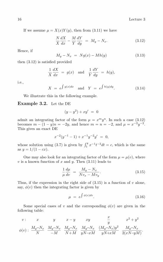
One may also look for an integrating factor of the form µ = µ(v), wherev is a known function of x and y. Then (3.11) leads to
1µ
dµ
dv=
My −Nx
Nvx −Mvy. (3.15)
Thus, if the expression in the right side of (3.15) is a function of v alone,say, φ(v) then the integrating factor is given by
µ = e∫
φ(v)dv. (3.16)
Some special cases of v and the corresponding φ(v) are given in thefollowing table:
v : x y x− y xyx
yx2 + y2
φ(v) :My−Nx
N
My−Nx
−MMy−Nx
N+MMy−Nx
yN−xM(My−Nx)y2
yN+xMMy−Nx
2(xN−yM).

Exact Equations 17
If the expression in the second row is a function of the corresponding vin the first row, then (3.1) has the integrating factor µ given in (3.16).
Example 3.3. For the DE
(x2y + y + 1) + x(1 + x2)y′ = 0,
we have
My −Nx
N=
1x(1 + x2)
(x2 + 1 − 1 − 3x2) = − 2x1 + x2 ,
which is a function of x. Hence, from the above table and (3.16) we findµ = (1 + x2)−1. Thus, the DE(
y +1
1 + x2
)+ xy′ = 0
is exact whose solution is given by xy + tan−1 x = c.
Example 3.4. For the DE in Example 3.2, we have
My −Nx
−M =2
1 − y,
which is a function of y. Hence, from the above table and (3.16) we findµ = (1 − y)−2. Thus, the DE
y
1 − y+
x
(1 − y)2y′ = 0
is exact whose solution is once again given by y = 1/(1 − cx).
Example 3.5. For the DE
(xy3 + 2x2y2 − y2) + (x2y2 + 2x3y − 2x2)y′ = 0,
we haveMy −Nx
yN − xM= 1 − 2
xy,
which is a function of xy. Hence, from the above table and (3.16) we findµ = x−2y−2exy. The resulting exact DE
(yx−1 + 2 − x−2)exy + (1 + 2xy−1 − 2y−2)exyy′ = 0
has a solution exy(x−1 + 2y−1) = c.
Next we shall prove an interesting result which enables us to find thesolution of (3.1) provided it admits two linearly independent integratingfactors. For this, we need the following lemma.

18 Lecture 3
Lemma 3.3. Suppose (3.1) is exact and has an integrating factorµ(x, y) (= constant), then µ(x, y) = c is a solution of (3.1).
Proof. In view of the hypothesis, condition (3.11) implies that Nµx =Mµy. Multiplying (3.1) by µy, we find
Mµy +Nµyy′ = N(µx + µyy
′) = Ndµ
dx= 0
and this implies the lemma.
Theorem 3.4. If µ1(x, y) and µ2(x, y) are two integrating factors of(3.1) such that their ratio is not a constant, then µ1(x, y) = cµ2(x, y) is asolution of (3.1).
Proof. Clearly, the DEs (i) µ1M+µ1Ny′ = 0, and (ii) µ2M+µ2Ny
′ = 0are exact. Multiplication of (ii) by µ1/µ2 converts it to the exact equa-tion (i). Thus, the exact DE (ii) admits an integrating factor µ1/µ2 andLemma 3.3 implies that µ1/µ2 = c is a solution of (ii), i.e., of (3.1).
To illustrate the importance of Theorem 3.4, we consider the DE inExample 3.2. It has two integrating factors, µ1 = x−2y−2 and µ2 = (1 −y)−2, which are obtained in Examples 3.2 and 3.4, respectively. Hence, itssolution is given by (1−y)2 = c2x2y2, which is the same as the one obtainedin Example 3.2, as it should be.
We finish this lecture with the remark that, generally, integrating factorsof (3.1) are obtained by “trial-and-error” methods.
Problems
3.1. Let the hypothesis of Theorem 3.1 be satisfied and the equation(3.1) be exact. Show that the solution of the DE (3.1) is given by∫ x
x0
M(s, y)ds+∫ y
y0
N(x0, t)dt = c.
3.2. Solve the following initial value problems:
(i) (3x2y + 8xy2) + (x3 + 8x2y + 12y2)y′ = 0, y(2) = 1.(ii) (4x3ex+y + x4ex+y + 2x) + (x4ex+y + 2y)y′ = 0, y(0) = 1.(iii) (x− y cosx) − sinxy′ = 0, y(π/2) = 1.(iv) (yexy + 4y3) + (xexy + 12xy2 − 2y)y′ = 0, y(0) = 2.
3.3. In the following DEs determine the constant a so that each equa-tion is exact, and solve the resulting DEs:

Exact Equations 19
(i) (x3 + 3xy) + (ax2 + 4y)y′ = 0.
(ii) (x−2 + y−2) + (ax+ 1)y−3y′ = 0.
3.4. The DE (ex sec y− tan y) + y′ = 0 has an integrating factor of theform e−ax cos y for some constant a. Find a, and then solve the DE.
3.5. The DE (4x + 3y2) + 2xyy′ = 0 has an integrating factor of theform xn, where n is a positive integer. Find n, and then solve the DE.
3.6. Verify that (x2 +y2)−1 is an integrating factor of a DE of the form(y + xf(x2 + y2)) + (yf(x2 + y2) − x)y′ = 0. Hence, solve the DE
(y + x(x2 + y2)2) + (y(x2 + y2)2 − x)y′ = 0.
3.7. If p and q are functions of x, then the DE (py − qyn) + y′ = 0admits an integrating factor of the form X(x)Y (y). Find the functions Xand Y.
3.8. Solve the following DEs for which the type of integrating factorhas been indicated:
(i) (x− y2) + 2xyy′ = 0 [µ(x)].
(ii) y + (y2 − x)y′ = 0 [µ(y)].
(iii) y + x(1 − 3x2y2)y′ = 0 [µ(xy)].
(iv) (3xy + y2) + (3xy + x2)y′ = 0 [µ(x+ y)].
(v) (x+ x4 + 2x2y2 + y4) + yy′ = 0 [µ(x2 + y2)].
(vi) (4xy + 3y4) + (2x2 + 5xy3)y′ = 0 [µ(xmyn)].
3.9. By differentiating the equation
∫g(xy) + h(xy)g(xy) − h(xy)
d(xy)(xy)
+ ln(x
y
)= c
with respect to x, verify that 2/(xy(g(xy)−h(xy))) is an integrating factorof the DE yg(xy) + xh(xy)y′ = 0. Hence, solve the DE
(x2y2 + xy + 1)y + (x2y2 − xy + 1)xy′ = 0.
3.10. Show the following:
(i) u(x, y) = c is the general solution of the DE (3.1) if and only ifMuy = Nux.
(ii) The DE (3.1) has an integrating factor (M2 +N2)−1 if Mx = Ny andMy = −Nx.

20 Lecture 3
Answers or Hints
3.1. Begin with uy = N and obtain an analog of (3.7).
3.2. (i) x3y+4x2y2+4y3 = 28. (ii) x4ex+y+x2+y2 = 1. (iii) x2−2y sinx =(π2/4) − 2. (iv) exy + 4xy3 − y2 + 3 = 0.
3.3. (i) 3/2, x4 + 6x2y + 8y2 = c. (ii) −2, y2 = x(2x− 1)/[2(cx+ 1)].
3.4. 1, sin−1((c− x)ex).
3.5. 2, x4 + x3y2 = c.
3.6. 4 tan−1(x/y) + (x2 + y2)2 = c.
3.7. exp((1 − n)
∫pdx
), y−n.
3.8. (i) x−2, y2 + x lnx = cx. (ii) y−2, y2 + x = cy. (iii) (xy)−3, y6 =c exp(−x−2y−2). (iv) (x+y), x3y+2x2y2 +xy3 = c, x+y = 0. (v) (x2 +y2)−2, (c+ 2x)(x2 + y2) = 1. (vi) x2y, x4y2 + x3y5 = c.
3.9. xy + ln(x/y) = c+ 1/(xy).
3.10. (i) Note that ux + yyy′ = 0 and M + Ny′ = 0. (ii) Mx = Ny and
My = −Nx imply ∂∂y
(M
M2+N2
)= ∂
∂x
(N
M2+N2
).

Lecture 4Elementary First-Order
Equations
Suppose in the DE of first order (3.1), M(x, y) = X1(x)Y1(y) andN(x, y) = X2(x)Y2(y), so that it takes the form
X1(x)Y1(y) +X2(x)Y2(y)y′ = 0. (4.1)
If Y1(y)X2(x) = 0 for all (x, y) ∈ S, then (4.1) can be written as an exact DE
X1(x)X2(x)
+Y2(y)Y1(y)
y′ = 0 (4.2)
in which the variables are separated. Such a DE (4.2) is said to be separable.The solution of this exact equation is given by∫
X1(x)X2(x)
dx+∫Y2(y)Y1(y)
dy = c. (4.3)
Here both the integrals are indefinite and constants of integration have beenabsorbed in c.
Equation (4.3) contains all the solutions of (4.1) for which Y1(y)X2(x) =0. In fact, when we divide (4.1) by Y1X2 we might have lost some solutions,and the ones which are not in (4.3) for some c must be coupled with (4.3)to obtain all solutions of (4.1).
Example 4.1. The DE in Example 3.2 may be written as
1x
+1
y(1 − y)y′ = 0, xy(1 − y) = 0
for which (4.3) gives the solution y = (1−cx)−1. Other possible solutions forwhich x(y−y2) = 0 are x = 0, y = 0, and y = 1. However, the solution y = 1is already included in y = (1 − cx)−1 for c = 0, and x = 0 is not a solution,and hence all solutions of this DE are given by y = 0, y = (1 − cx)−1.
A function f(x, y) defined in a domain D (an open connected set in IR2)is said to be homogeneous of degree k if for all real λ and (x, y) ∈ D
f(λx, λy) = λkf(x, y). (4.4)
R.P. Agarwal and D. O’Regan, An Introduction to Ordinary Differential Equations,
4 , © Springer Science + Business Media, LLC 2008 doi: 10.1007/978-0-387-71276-5_
21

22 Lecture 4
For example, the functions 3x2 − xy − y2, sin(x2/(x2 − y2)), (x4 +7y4)1/5, (1/x2) sin(x/y) + (x/y3)(ln y− lnx), and (6ey/x/x2/3y1/3) are ho-mogeneous of degree 2, 0, 4/5, − 2, and −1, respectively.
In (4.4) if λ = 1/x, then it is the same as
xkf(1,y
x
)= f(x, y). (4.5)
This implies that a homogeneous function of degree zero is a function of asingle variable v (= y/x).
The first-order DE (3.1) is said to be homogeneous if M(x, y) andN(x, y) are homogeneous functions of the same degree, say, n. If (3.1) ishomogeneous, then in view of (4.5) it can be written as
xnM(1,y
x
)+ xnN
(1,y
x
)y′ = 0. (4.6)
In (4.6) we use the substitution y(x) = xv(x), to obtain
xn(M(1, v) + vN(1, v)) + xn+1N(1, v)v′ = 0. (4.7)
Equation (4.7) is separable and admits the integrating factor
µ =1
xn+1(M(1, v) + vN(1, v))=
1xM(x, y) + yN(x, y)
(4.8)
provided xM + yN = 0.
The vanishing of xM + yN implies that (4.7) is simply
xn+1N(1, v)v′ = xN(x, y)v′ = 0
for which the integrating factor is 1/xN. Thus, in this case the generalsolution of (3.1) is given by y = cx.
We summarize these results in the following theorem.
Theorem 4.1. The homogeneous DE (4.6) can be transformed to aseparable DE by the transformation y = xv which admits an integratingfactor 1/(xM + yN) provided xM + yN = 0. Further, if xM + yN = 0,then its integrating factor is 1/xN and it has y = cx as its general solution.
Example 4.2. The DE
y′ =x2 + xy + y2
x2 , x = 0

Elementary First-Order Equations 23
is homogeneous. The transformation y = xv simplifies this DE to xv′ =1 + v2. Thus, tan−1(y/x) = ln |cx| is the general solution of the given DE.Alternatively, the integrating factor
[x
(x2 + xy + y2
x2
)− y
]−1
=(x2 + y2
x
)−1
converts the given DE into the exact equation
1x
+y
x2 + y2 − x
x2 + y2 y′ = 0
whose general solution using (3.7) is given by − tan−1(y/x) + lnx = c,which is the same as obtained earlier.
Often, it is possible to introduce a new set of variables given by theequations
u = φ(x, y), v = ψ(x, y) (4.9)
which convert a given DE (1.9) into a form that can be solved rather easily.Geometrically, relations (4.9) can be regarded as a mapping of a region inthe xy-plane into the uv-plane. We wish to be able to solve these relationsfor x and y in terms of u and v. For this, we should assume that the mappingis one-to-one. In other words, we can assume that ∂(u, v)/∂(x, y) = 0 over aregion in IR2, which implies that there is no functional relationship betweenu and v. Thus, if (u0, v0) is the image of (x0, y0) under the transformation(4.9), then it can be uniquely solved for x and y in a neighborhood of thepoint (x0, y0). This leads to the inverse transformation
x = x(u, v), y = y(u, v). (4.10)
The image of a curve in the xy-plane is a curve in the uv-plane; and therelation between slopes at the corresponding points of these curves is
y′ =yu + yv
dv
du
xu + xvdv
du
. (4.11)
Relations (4.10) and (4.11) can be used to convert the DE (1.9) in terms ofu and v, which hopefully can be solved explicitly. Finally, replacement ofu and v in terms of x and y by using (4.9) leads to an implicit solution ofthe DE (1.9).
Unfortunately, for a given nonlinear DE there is no way to predict atransformation which leads to a solution of (1.9). Finding such a trans-formation can only be learned by practice. We therefore illustrate thistechnique in the following examples.

24 Lecture 4
Example 4.3. Consider the DE
3x2yey + x3ey(y + 1)y′ = 0.
Setting u = x3, v = yey we obtain
3x2 dv
dy= ey(y + 1)
du
dx,
and this changes the given DE into the form v + u(dv/du) = 0 for whichthe solution is uv = c, equivalently, x3yey = c is the general solution of thegiven DE.
We now consider the DE
y′ = f
(a1x+ b1y + c1a2x+ b2y + c2
)(4.12)
in which a1, b1, c1, a2, b2 and c2 are constants. If c1 and c2 are not bothzero, then it can be converted to a homogeneous equation by means of thetransformation
x = u+ h, y = v + k (4.13)
where h and k are the solutions of the system of simultaneous linear equa-tions
a1h+ b1k + c1 = 0a2h+ b2k + c2 = 0, (4.14)
and the resulting homogeneous DE
dv
du= f
(a1u+ b1v
a2u+ b2v
)(4.15)
can be solved easily.
However, the system (4.14) can be solved for h and k provided ∆ =a1b2 − a2b1 = 0. If ∆ = 0, then a1x+ b1y is proportional to a2x+ b2y, andhence (4.12) is of the form
y′ = f(αx+ βy), (4.16)
which can be solved easily by using the substitution αx+ βy = z.
Example 4.4. Consider the DE
y′ =12
(x+ y − 1x+ 2
)2
.
The straight lines h + k − 1 = 0 and h + 2 = 0 intersect at (−2, 3), andhence the transformation x = u− 2, y = v+ 3 changes the given DE to theform
dv
du=
12
(u+ v
u
)2
,

Elementary First-Order Equations 25
which has the solution 2 tan−1(v/u) = ln |u| + c, and thus
2 tan−1 y − 3x+ 2
= ln |x+ 2| + c
is the general solution of the given DE.
Example 4.5. The DE
(x+ y + 1) + (2x+ 2y + 1)y′ = 0
suggests that we should use the substitution x + y = z. This converts thegiven DE to the form (2z + 1)z′ = z for which the solution is 2z + ln |z| =x+c, z = 0; or equivalently, x+2y+ln |x+y| = c, x+y = 0. If z = x+y = 0,then the given DE is satisfied by the relation x+ y = 0. Thus, all solutionsof the given DE are x+ 2y + ln |x+ y| = c, x+ y = 0.
Let f(x, y, α) = 0 and g(x, y, β) = 0 be the equations of two familiesof curves, each dependent on one parameter. When each member of thesecond family cuts each member of the first family according to a definitelaw, any curve of either of the families is said to be a trajectory of thefamily. The most important case is that in which curves of the familiesintersect at a constant angle. The orthogonal trajectories of a given familyof curves are the curves that cut the given family at right angles. The slopesy′1 and y′
2 of the tangents to the curves of the family and to the soughtfor orthogonal trajectories must at each point satisfy the orthogonalitycondition y′
1y′2 = −1.
Example 4.6. For the family of parabolas y = ax2, we have y′ = 2axor y′ = 2y/x. Thus, the DE of the desired orthogonal trajectories is y′ =−(x/2y). Separating the variables, we find 2yy′ +x = 0, and on integratingthis DE we obtain the family of ellipses x2 + 2y2 = c.
Problems
4.1. Show that if (3.1) is both homogeneous and exact, and Mx+Nyis not a constant, then its general solution is given by Mx+Ny = c.
4.2. Show that if the DE (3.1) is homogeneous and M and N possesscontinuous partial derivatives in some domain D, then
xMx + yMy
xNx + yNy=
M
N.
4.3. Solve the following DEs:
(i) x sin y + (x2 + 1) cos yy′ = 0.

26 Lecture 4
(ii) (x+ 2y − 1) + 3(x+ 2y)y′ = 0.(iii) xy′ − y = xey/x.
(iv) xy′ − y = x sin[(y − x)/x].(v) y′ = (x+ y + 1)2 − 2.(vi) y′ = (3x− y − 5)/(−x+ 3y + 7).
4.4. Use the given transformation to solve the following DEs:
(i) 3x5 − y(y2 − x3)y′ = 0, u = x3, v = y2.(ii) (2x+ y) + (x+ 5y)y′ = 0, u = x− y, v = x+ 2y.(iii) (x+ 2y) + (y − 2x)y′ = 0, x = r cos θ, y = r sin θ.(iv) (2x2 + 3y2 − 7)x− (3x2 + 2y2 − 8)yy′ = 0, u = x2, v = y2.
4.5. Show that the transformation y(x) = xv(x) converts the DEynf(x) + g(y/x)(y − xy′) = 0 into a separable equation.
4.6. Show that the change of variable y = xnv in the DE y′ =xn−1f(y/xn) leads to a separable equation. Hence, solve the DE
x3y′ = 2y(x2 − y).
4.7. Show that the introduction of polar coordinates x = r cos θ, y =r sin θ leads to separation of variables in a homogeneous DE y′ = f(y/x).Hence, solve the DE
y′ =ax+ by
bx− ay.
4.8. Solve
y′ =y − xy2
x+ x2y
by making the substitution y = vxn for an appropriate n.
4.9. Show that the families of parabolas y2 = 2cx+ c2, x2 = 4a(y+ a)are self-orthogonal.
4.10. Show that the circles x2+y2 = px intersect the circles x2+y2 = qyat right angles.
∗4.11. Show that if the functions f, fx, fy, and fxy are continuous onsome region D in the xy-plane, f is never zero on D, and ffxy = fxfy onD, then the DE (1.9) is separable. The requirement f(x, y) = 0 is essential,for this consider the function
f(x, y) =
x2e2y, y ≤ 0
x2ey, y > 0.

Elementary First-Order Equations 27
Answers or Hints
4.1. First use Theorem 4.1 and then Lemma 3.3.
4.2. Use Theorem 4.1.
4.3. (i) (x2 +1) sin2 y = c. (ii) x+3y+c = 3 ln(x+2y+2), x+2y+2 = 0.(iii) exp(−y/x) + ln |x| = c, x = 0. (iv) tan(y − x)/2x = cx, x = 0.(v) (x+ y + 1)(1 − ce2x) = 1 + ce2x. (vi) (x+ y + 1)2(y − x+ 3) = c.
4.4. (i) (y2−2x3)(y2+x3)2 = c. (ii) 2x2+2xy+5y2 = c. (iii)√x2 + y2 =
c exp(2 tan−1 y/x). (iv) (x2 − y2 − 1)5 = c(x2 + y2 − 3).
4.5. The given DE is reduced to vnxnf(x) = x2g(v)v′.
4.6. y(2 ln |x| + c) = x2, y = 0.
4.7.√x2 + y2 = c exp
(ba tan−1 y
x
).
4.8. yexy = cx.
4.9. For y2 = 2cx + c2, y′ = c/y and hence the DE for the orthogonaltrajectories is y′ = −y/c, but it can be shown that it is the same as y′ = c/y.
4.10. For the given families y′ = (y2 − x2)/2xy and y′ = 2xy/(x2 − y2),respectively.

Lecture 5First-Order Linear Equations
Let in the DE (3.1) the functions M and N be p1(x)y− r(x) and p0(x),respectively, then it becomes
p0(x)y′ + p1(x)y = r(x), (5.1)
which is a first-order linear DE. In (5.1) we shall assume that the func-tions p0(x), p1(x), r(x) are continuous and p0(x) = 0 in J. With theseassumptions the DE (5.1) can be written as
y′ + p(x)y = q(x), (5.2)
where p(x) = p1(x)/p0(x) and q(x) = r(x)/p0(x) are continuous functionsin J.
The corresponding homogeneous equation
y′ + p(x)y = 0 (5.3)
obtained by taking q(x) ≡ 0 in (5.2) can be solved by separating the vari-ables, i.e., (1/y)y′ + p(x) = 0, and now integrating it to obtain
y(x) = c exp(
−∫ x
p(t)dt). (5.4)
In dividing (5.3) by y we have lost the solution y(x) ≡ 0, which is called thetrivial solution (for a linear homogeneous DE y(x) ≡ 0 is always a solution).However, it is included in (5.4) with c = 0.
If x0 ∈ J, then the function
y(x) = y0 exp(
−∫ x
x0
p(t)dt)
(5.5)
clearly satisfies the DE (5.3) in J and passes through the point (x0, y0).Thus, it is the solution of the initial value problem (5.3), (1.10).
To find the solution of the DE (5.2) we shall use the method of variationof parameters due to Lagrange. In (5.4) we assume that c is a function ofx, i.e.,
y(x) = c(x) exp(
−∫ x
p(t)dt)
(5.6)
R.P. Agarwal and D. O’Regan, An Introduction to Ordinary Differential Equations,
doi: 10.1007/978-0-387-71276-5_5, © Springer Science + Business Media, LLC 2008
28

First-Order Linear Equations 29
and search for c(x) so that (5.6) becomes a solution of the DE (5.2). Forthis, substituting (5.6) into (5.2), we find
c′(x) exp(
−∫ x
p(t)dt)
−c(x)p(x) exp(
−∫ x
p(t)dt)
+c(x)p(x) exp(
−∫ x
p(t)dt)
= q(x),
which is the same as
c′(x) = q(x) exp(∫ x
p(t)dt). (5.7)
Integrating (5.7), we obtain the required function
c(x) = c1 +∫ x
q(t) exp(∫ t
p(s)ds)dt.
Now substituting this c(x) in (5.6), we find the solution of (5.2) as
y(x) = c1 exp(
−∫ x
p(t)dt)
+∫ x
q(t) exp(
−∫ x
t
p(s)ds)dt. (5.8)
This solution y(x) is of the form c1u(x) + v(x). It is to be noted thatc1u(x) is the general solution of (5.3) and v(x) is a particular solutionof (5.2). Hence, the general solution of (5.2) is obtained by adding anyparticular solution of (5.2) to the general solution of (5.3).
From (5.8) the solution of the initial value problem (5.2), (1.10) wherex0 ∈ J is easily obtained as
y(x) = y0 exp(
−∫ x
x0
p(t)dt)
+∫ x
x0
q(t) exp(
−∫ x
t
p(s)ds)dt. (5.9)
This solution in the particular case when p(x) ≡ p and q(x) ≡ q simplyreduces to
y(x) =(y0 − q
p
)e−p(x−x0) +
q
p.
Example 5.1. Consider the initial value problem
xy′ − 4y + 2x2 + 4 = 0, x = 0, y(1) = 1. (5.10)
Since x0 = 1, y0 = 1, p(x) = −4/x and q(x) = −2x− 4/x, from (5.9) the

30 Lecture 5
solution of (5.10) can be written as
y(x) = exp(∫ x
1
4tdt
)+∫ x
1
(−2t− 4
t
)exp
(∫ x
t
4sds
)dt
= x4 +∫ x
1
(−2t− 4
t
)x4
t4dt
= x4 + x4(
1x2 +
1x4 − 2
)= − x4 + x2 + 1.
Alternatively, instead of using (5.9), we can find the solution of (5.10) asfollows. For the corresponding homogeneous DE y′−(4/x)y = 0 the generalsolution is cx4, and a particular solution of the DE (5.10) is∫ x(
−2t− 4t
)exp
(∫ x
t
4sds
)dt = x2 + 1,
and hence the general solution of the DE (5.10) is y(x) = cx4+x2+1. Now inorder to satisfy the initial condition y(1) = 1 it is necessary that 1 = c+1+1,or c = −1. The solution of (5.10) is therefore y(x) = −x4 + x2 + 1.
Suppose y1(x) and y2(x) are two particular solutions of (5.2), then
y′1(x) − y′
2(x) = −p(x)y1(x) + q(x) + p(x)y2(x) − q(x)
= −p(x)(y1(x) − y2(x)),
which implies that y(x) = y1(x) − y2(x) is a solution of (5.3). Thus, if twoparticular solutions of (5.2) are known, then y(x) = c(y1(x)−y2(x))+y1(x)as well as y(x) = c(y1(x)− y2(x))+ y2(x) represents the general solution of(5.2). For example, x+1/x and x are two solutions of the DE xy′ + y = 2xand y(x) = c/x+ x is its general solution.
The DE (xf(y) + g(y))y′ = h(y) may not be integrable as it is, but ifthe roles of x and y are interchanged, then it can be written as
h(y)dx
dy− f(y)x = g(y),
which is a linear DE in x and can be solved by the preceding procedure.In fact, the solutions of (1.9) and dx/dy = 1/f(x, y) determine the samecurve in a region in IR2 provided the function f is defined, continuous,and nonzero. For this, if y = y(x) is a solution of (1.9) in J and y′(x) =f(x, y(x)) = 0, then y(x) is monotonic function in J and hence has aninverse x = x(y). This function x is such that
dx
dy=
1y′(x)
=1
f(x, y(x))in J.

First-Order Linear Equations 31
Example 5.2. The DE
y′ =1
(e−y − x)
can be written as dx/dy + x = e−y which can be solved to obtain x =e−y(y + c).
Certain nonlinear first-order DEs can be reduced to linear equations byan appropriate change of variables. For example, it is always possible forthe Bernoulli equation
p0(x)y′ + p1(x)y = r(x)yn, n = 0, 1. (5.11)
In (5.11), n = 0 and 1 are excluded because in these cases this equation isobviously linear.
The equation (5.11) is equivalent to the DE
p0(x)y−ny′ + p1(x)y1−n = r(x) (5.12)
and now the substitution v = y1−n leads to the first-order linear DE
11 − n
p0(x)v′ + p1(x)v = r(x). (5.13)
Example 5.3. The DE xy′ + y = x2y2, x = 0 can be written asxy−2y′ + y−1 = x2. The substitution v = y−1 converts this DE into −xv′ +v = x2, which can be solved to get v = (c − x)x, and hence the generalsolution of the given DE is y(x) = (cx− x2)−1.
As we have remarked in Lecture 2, we shall show that if one solutiony1(x) of the Riccati equation (2.14) is known, then the substitution y =y1 + z−1 converts it into a first-order linear DE in z. Indeed, we have
y′1 − 1
z2 z′ = p(x)
(y1 +
1z
)2
+ q(x)(y1 +
1z
)+ r(x)
= (p(x)y21 + q(x)y1 + r(x)) + p(x)
(2y1z
+1z2
)+ q(x)
1z
and hence− 1z2 z
′ = (2p(x)y1 + q(x))1z
+ p(x)1z2 ,
which is the first-order linear DE
z′ + (2p(x)y1 + q(x))z + p(x) = 0. (5.14)
Example 5.4. It is easy to verify that y1 = x is a particular solution ofthe Riccati equation y′ = 1 + x2 − 2xy + y2. The substitution y = x+ z−1

32 Lecture 5
converts this DE to the first-order linear DE z′ + 1 = 0, whose generalsolution is z = (c − x), x = c. Thus, the general solution of the givenRiccati equation is y(x) = x+ 1/(c− x), x = c.
In many physical problems the nonhomogeneous term q(x) in (5.2) isspecified by different formulas in different intervals. This is often the casewhen (5.2) is considered as an input–output relation, i.e., the function q(x)is an input and the solution y(x) is an output corresponding to the inputq(x). Usually, in such situations the solution y(x) is not defined at certainpoints, so that it is not continuous throughout the interval of interest. Tounderstand such a case, for simplicity, we consider the initial value problem(5.2), (1.10) in the interval [x0, x2], where the function p(x) is continuous,and
q(x) =
q1(x), x0 ≤ x < x1
q2(x), x1 < x ≤ x2.
We assume that the functions q1(x) and q2(x) are continuous in the intervals[x0, x1) and (x1, x2], respectively. With these assumptions the “solution”y(x) of (5.2), (1.10) in view of (5.9) can be written as
y(x) =
⎧⎪⎪⎪⎪⎪⎪⎨⎪⎪⎪⎪⎪⎪⎩
y1(x) = y0 exp(
−∫ x
x0
p(t)dt)
+∫ x
x0
q1(t) exp(
−∫ x
t
p(s)ds)dt,
x0 ≤ x < x1
y2(x) = c exp(
−∫ x
x1
p(t)dt)
+∫ x
x1
q2(t) exp(
−∫ x
t
p(s)ds)dt,
x1 < x ≤ x2.
Clearly, at the point x1 we cannot say much about the solution y(x),it may not even be defined. However, if the limits limx→x−
1y1(x) and
limx→x+1y2(x) exist (which are guaranteed if both the functions q1(x) and
q2(x) are bounded at x = x1), then the relation
limx→x−
1
y1(x) = limx→x+
1
y2(x) (5.15)
determines the constant c, so that the solution y(x) is continuous on [x0, x2].
Example 5.5. Consider the initial value problem
y′ − 4xy =
⎧⎨⎩ −2x− 4
x, x ∈ [1, 2)
x2, x ∈ (2, 4]
y(1) = 1.
(5.16)
In view of Example 5.1 the solution of (5.16) can be written as
y(x) =
⎧⎨⎩
−x4 + x2 + 1, x ∈ [1, 2)
cx4
16+x4
2− x3, x ∈ (2, 4].

First-Order Linear Equations 33
Now the relation (5.15) gives c = −11. Thus, the continuous solution of(5.16) is
y(x) =
⎧⎨⎩
−x4 + x2 + 1, x ∈ [1, 2)
− 316x4 − x3, x ∈ (2, 4].
Clearly, this solution is not differentiable at x = 2.
Problems
5.1. Show that the DE (5.2) admits an integrating factor which is afunction of x alone. Use this to obtain its general solution.
5.2. (Principle of Superposition). If y1(x) and y2(x) are solutions ofy′ + p(x)y = qi(x), i = 1, 2, respectively, then show that c1y1(x) + c2y2(x)is a solution of the DE y′ + p(x)y = c1q1(x) + c2q2(x), where c1 and c2 areconstants.
5.3. Find the general solution of the following DEs:
(i) y′ − (cotx)y = 2x sinx.(ii) y′ + y + x+ x2 + x3 = 0.(iii) (y2 − 1) + 2(x− y(1 + y)2)y′ = 0.(iv) (1 + y2) = (tan−1 y − x)y′.
5.4. Solve the following initial value problems:
(i) y′ + 2y =
1, 0 ≤ x ≤ 10, x > 1 , y(0) = 0.
(ii) y′ + p(x)y = 0, y(0) = 1, where p(x) =
2, 0 ≤ x ≤ 11, x > 1.
5.5. Let q(x) be continuous in [0,∞) and limx→∞ q(x) = L. For theDE y′ + ay = q(x), show the following:
(i) If a > 0, every solution approaches L/a as x → ∞.(ii) If a < 0, there is one and only one solution which approaches L/a asx → ∞.
5.6. Let y(x) be the solution of the initial value problem (5.2), (1.10)in [x0,∞), and let z(x) be a continuously differentiable function in [x0,∞)such that z′ + p(x)z ≤ q(x), z(x0) ≤ y0. Show that z(x) ≤ y(x) for all x in[x0,∞). In particular, for the problem y′ + y = cosx, y(0) = 1 verify that2e−x − 1 ≤ y(x) ≤ 1, x ∈ [0,∞).
5.7. Find the general solution of the following nonlinear DEs:

34 Lecture 5
(i) 2(1 + y3) + 3xy2y′ = 0.(ii) y + x(1 + xy4)y′ = 0.(iii) (1 − x2)y′ + y2 − 1 = 0.(iv) y′ − e−xy2 − y − ex = 0.
∗5.8. Let the functions p0, p1, and r be continuous in J = [α, β] suchthat p0(α) = p0(β) = 0, p0(x) > 0, x ∈ (α, β), p1(x) > 0, x ∈ J, and
∫ α+ε
α
dx
p0(x)=
∫ β
β−ε
dx
p0(x)= ∞, 0 < ε < β − α.
Show that all solutions of the DE (5.1) which exist in (α, β) converge tor(β)/p1(β) as x → β. Further, show that one of these solutions convergesto r(α)/p1(α) as x → α, while all other solutions converge to ∞, or −∞.
Answers or Hints
5.1. Since M = p(x)y − q(x), N = 1, [(My −Nx)/N ] = p(x), and hencethe integrating factor is exp(
∫ xp(t)dt).
5.2. Use the definition of a solution.
5.3. (i) c sinx+x2 sinx. (ii) ce−x−x3+2x2−5x+5. (iii) x(y−1)/(y+1) =y2 + c. (iv) x = tan−1 y − 1 + ce− tan−1 y.
5.4. (i) y(x) = 1
2 (1 − e−2x), 0 ≤ x ≤ 112 (e2 − 1)e−2x, x > 1
(ii) y(x) =e−2x, 0 ≤ x ≤ 1e−(x+1), x > 1.
5.5. (i) In y(x) = y(x0)e−a(x−x0) + [∫ x
x0eatq(t)dt]/eax take the limit x →
∞. (ii) In y(x) = e−ax[y(x0)eax0 +
∫∞x0eatq(t)dt− ∫∞
xeatq(t)dt
]choose
y(x0) so that y(x0)eax0 +∫∞
x0eatq(t)dt = 0 (limx→∞ q(x) = L). Now in
y(x) = −[∫∞
xeatq(t)dt]/eax take the limit x → ∞.
5.6. There exists a continuous function r(x) ≥ 0 such that z′ + p(x)z =q(x) − r(x), z(x0) ≤ y0. Thus, for the function φ(x) = y(x) − z(x), φ′ +p(x)φ = r(x) ≥ 0, φ(x0) = y0 − z(x0) ≥ 0.
5.7. (i) x2(1+ y3) = c. (ii) xy4 = 3(1+ cxy), y = 0. (iii) (y− 1)(1+x) =c(1 − x)(1 + y). (iv) ex tan(x+ c).

Lecture 6Second-Order Linear Equations
Consider the homogeneous linear second-order DE with variable coeffi-cients
p0(x)y′′ + p1(x)y′ + p2(x)y = 0, (6.1)
where p0(x) (> 0), p1(x) and p2(x) are continuous in J. There does not existany method to solve it except in a few rather restrictive cases. However,the results below follow immediately from the general theory of first-orderlinear systems, which we shall present in later lectures.
Theorem 6.1. There exist exactly two solutions y1(x) and y2(x) of(6.1) which are linearly independent (essentially different) in J ; i.e., theredoes not exist a constant c such that y1(x) = cy2(x) for all x ∈ J.
Theorem 6.2. Two solutions y1(x) and y2(x) of (6.1) are linearlyindependent in J if and only if their Wronskian defined by
W (x) = W (y1, y2)(x) =∣∣∣∣ y1(x) y2(x)y′1(x) y′
2(x)
∣∣∣∣ = y1(x)y′2(x) − y2(x)y′
1(x)
(6.2)is different from zero for some x = x0 in J.
Theorem 6.3. For the Wronskian defined in (6.2) the following Abel’sidentity (also known as the Ostrogradsky–Liouville formula) holds:
W (x) = W (x0) exp(
−∫ x
x0
p1(t)p0(t)
dt
), x0 ∈ J. (6.3)
Thus, if the Wronskian is zero at some x0 ∈ J, then it is zero for all x ∈ J.
Theorem 6.4. If y1(x) and y2(x) are solutions of (6.1) and c1 and c2are arbitrary constants, then c1y1(x) + c2y2(x) is also a solution of (6.1).Further, if y1(x) and y2(x) are linearly independent, then any solution y(x)of (6.1) can be written as y(x) = c1y1(x) + c2y2(x), where c1 and c2 aresuitable constants.
Now we shall show that, if one solution y1(x) of (6.1) is known (bysome clever method), then we can employ variation of parameters to findthe second solution of (6.1). For this we let y(x) = u(x)y1(x) and substitutethis in (6.1) to get
p0(uy1)′′ + p1(uy1)′ + p2(uy1) = 0,
R.P. Agarwal and D. O’Regan, An Introduction to Ordinary Differential Equations,
doi: 10.1007/978-0-387-71276-5_6, © Springer Science + Business Media, LLC 2008
35

36 Lecture 6
orp0u
′′y1 + 2p0u′y′
1 + p0uy′′1 + p1u
′y1 + p1uy′1 + p2uy1 = 0,
orp0u
′′y1 + (2p0y′1 + p1y1)u′ + (p0y
′′1 + p1y
′1 + p2y1)u = 0.
However, since y1 is a solution of (6.1), the above equation with v = u′ isthe same as
p0y1v′ + (2p0y
′1 + p1y1)v = 0, (6.4)
which is a first-order equation, and it can be solved easily provided y1 = 0in J. Indeed, multiplying (6.4) by y1/p0, we get
(y21v
′ + 2y′1y1v) +
p1
p0y21v = 0,
which is the same as(y2
1v)′ +
p1
p0(y2
1v) = 0
and hence
y21v = c exp
(−∫ x p1(t)
p0(t)dt
),
or, on taking c = 1,
v(x) =1
y21(x)
exp(
−∫ x p1(t)
p0(t)dt
).
Hence, the second solution of (6.1) is
y2(x) = y1(x)∫ x 1
y21(t)
exp(
−∫ t p1(s)
p0(s)ds
)dt. (6.5)
Example 6.1. It is easy to verify that y1(x) = x2 is a solution ofthe DE
x2y′′ − 2xy′ + 2y = 0, x = 0.
For the second solution we use (6.5), to obtain
y2(x) = x2∫ x 1
t4exp
(−∫ t(
−2ss2
)ds
)dt = x2
∫ x 1t4t2dt = − x.
Now we shall find a particular solution of the nonhomogeneous equation
p0(x)y′′ + p1(x)y′ + p2(x)y = r(x). (6.6)
For this also we shall apply the method of variation of parameters. Lety1(x) and y2(x) be two solutions of (6.1). We assume y(x) = c1(x)y1(x) +c2(x)y2(x) is a solution of (6.6). Note that c1(x) and c2(x) are two unknown

Second-Order Linear Equations 37
functions, so we can have two sets of conditions which determine c1(x) andc2(x). Since
y′ = c1y′1 + c2y
′2 + c′1y1 + c′2y2
as a first condition, we assume that
c′1y1 + c′2y2 = 0. (6.7)
Thus, we havey′ = c1y
′1 + c2y
′2
and on differentiation
y′′ = c1y′′1 + c2y
′′2 + c′1y
′1 + c′2y
′2.
Substituting these in (6.6), we find
c1(p0y′′1 + p1y
′1 + p2y1) + c2(p0y
′′2 + p1y
′2 + p2y2) + p0(c′1y
′1 + c′2y
′2) = r(x).
Clearly, this equation in view of the fact that y1(x) and y2(x) are solutionsof (6.1) is the same as
c′1y′1 + c′2y
′2 =
r(x)p0(x)
. (6.8)
Solving (6.7), (6.8) we find
c′1 = − y2(x)r(x)/p0(x)∣∣∣∣ y1(x) y2(x)y′1(x) y′
2(x)
∣∣∣∣, c′2 =
y1(x)r(x)/p0(x)∣∣∣∣ y1(x) y2(x)y′1(x) y′
2(x)
∣∣∣∣;
and hence a particular solution of (6.6) is
yp(x) = c1(x)y1(x) + c2(x)y2(x)
= −y1(x)∫ x y2(t)r(t)/p0(t)∣∣∣∣ y1(t) y2(t)
y′1(t) y′
2(t)
∣∣∣∣dt + y2(x)
∫ x y1(t)r(t)/p0(t)∣∣∣∣ y1(t) y2(t)y′1(t) y′
2(t)
∣∣∣∣dt
=∫ x
H(x, t)r(t)p0(t)
dt,
(6.9)where
H(x, t) =∣∣∣∣ y1(t) y2(t)y1(x) y2(x)
∣∣∣∣/ ∣∣∣∣ y1(t) y2(t)
y′1(t) y′
2(t)
∣∣∣∣ . (6.10)
The general solution of (6.6) which is obtained by adding this particularsolution with the general solution of (6.1) appears as
y(x) = c1y1(x) + c2y2(x) + yp(x). (6.11)

38 Lecture 6
The following properties of the function H(x, t) are immediate:
(i) H(x, t) is defined for all (x, t) ∈ J × J ;
(ii) ∂jH(x, t)/∂xj , j = 0, 1, 2 are continuous for all (x, t) ∈ J × J ;
(iii) for each fixed t ∈ J the function z(x) = H(x, t) is a solution of thehomogeneous DE (6.1) satisfying z(t) = 0, z′(t) = 1; and
(iv) the function
v(x) =∫ x
x0
H(x, t)r(t)p0(t)
dt
is a particular solution of the nonhomogeneous DE (6.6) satisfying y(x0) =y′(x0) = 0.
Example 6.2. Consider the DE
y′′ + y = cotx.
For the corresponding homogeneous DE y′′ +y = 0, sinx and cosx are thesolutions. Thus, its general solution can be written as
y(x) = c1 cosx+ c2 sinx+∫ x
∣∣∣∣ sin t cos tsinx cosx
∣∣∣∣∣∣∣∣ sin t cos tcos t − sin t
∣∣∣∣cos tsin t
dt
= c1 cosx+ c2 sinx−∫ x
(sin t cosx− sinx cos t)cos tsin t
dt
= c1 cosx+ c2 sinx− cosx∫ x
cos tdt+ sinx∫ x cos2 t
sin tdt
= c1 cosx+ c2 sinx− cosx sinx+ sinx∫ x 1 − sin2 t
sin tdt
= c1 cosx+ c2 sinx− cosx sinx− sinx∫ x
sin tdt+ sinx∫ x 1
sin tdt
= c1 cosx+ c2 sinx+ sinx∫ x cosec t(cosec t− cot t)
(cosec t− cot t)dt
= c1 cosx+ c2 sinx+ sinx ln[cosecx− cotx].
From the general theory of first-order linear systems, which we shallpresent in later lectures, it also follows that if the functions p0(x) (> 0),p1(x), p2(x), and r(x) are continuous on J and x0 ∈ J, then the initialvalue problem: (6.6) together with the initial conditions
y(x0) = y0, y′(x0) = y1 (6.12)
has a unique solution.

Second-Order Linear Equations 39
Now we shall show that second-order DEs with constant coefficients canbe solved explicitly. In fact, to find the solution of the equation
y′′ + ay′ + by = 0, (6.13)
where a and b are constants, as a first step we look back at the equationy′ + ay = 0 (a is a constant) for which all solutions are multiples of y =e−ax. Thus, for (6.13) also some form of exponential function would be areasonable choice and would utilize the property that the differentiation ofan exponential function erx always yields a constant multiplied by erx.
Thus, we try y = erx and find the value(s) of r. For this, we have
r2erx + arerx + berx = (r2 + ar + b)erx = 0,
which givesr2 + ar + b = 0. (6.14)
Hence, erx is a solution of (6.13) if r is a solution of (6.14). Equation (6.14)is called the characteristic equation. For the roots of (6.14) we have thefollowing three cases:
1. Distinct real roots. If r1 and r2 are real and distinct roots of(6.14), then er1x and er2x are two solutions of (6.13) and its general solutioncan be written as
y(x) = c1er1x + c2e
r2x.
In the particular case when r1 = r, r2 = −r (then the DE (6.13) is y′′ −r2y = 0) we have
y(x) = c1erx + c2e
−rx =(A+B
2
)erx +
(A−B
2
)e−rx
= A
(erx + e−rx
2
)+B
(erx − e−rx
2
)= A cosh rx+B sinh rx.
2. Repeated real roots. If r1 = r2 = r is a repeated root of(6.14), then erx is a solution. To find the second solution, we let y(x) =u(x)erx and substitute it in (6.13), to get
erx(u′′ + 2ru′ + r2u) + aeru(u′ + ru) + buerx = 0,
oru′′ + (2r + a)u′ + (r2 + ar + b)u = u′′ + (2r + a)u′ = 0.
Now since r is a repeated root of (6.14) it follows that 2r+a = 0 and henceu′′ = 0, i.e., u(x) = c1 + c2x. Thus,
y(x) = (c1 + c2x)erx = c1erx + c2xe
rx.

40 Lecture 6
Hence, the second solution of (6.13) is xerx.
3. Complex conjugate roots. Let r1 = µ+ iν and r2 = µ− iνwhere i =
√−1, so that
e(µ±iν)x = eµx(cos νx± i sin νx).
Since for the DE (6.13) real part, i.e., eµx cos νx and the complex part, i.e.,eµx sin νx both are solutions, the general solution of (6.13) can be writtenas
y(x) = c1eµx cos νx+ c2e
µx sin νx.
In the particular case when r1 = iν and r2 = −iν (then the DE (6.13) isy′′ + ν2y = 0) we have y(x) = c1 cos νx+ c2 sin νx.
Finally, in this lecture we shall find the solution of the Cauchy–Eulerequation
x2y′′ + axy′ + by = 0, x > 0. (6.15)
We assume y(x) = xm to obtain
x2m(m− 1)xm−2 + axmxm−1 + bxm = 0,
orm(m− 1) + am+ b = 0. (6.16)
This is the characteristic equation for (6.15), and as earlier for (6.14) thenature of its roots determines the solution:
Real, distinct roots m1 = m2: y(x) = c1xm1 + c2x
m2 ,
Real, repeated roots m = m1 = m2: y(x) = c1xm + c2(lnx)xm,
Complex conjugate roots m1 = µ + iν, m2 = µ − iν : y(x) =c1x
µ cos(ν lnx) + c2xµ sin(ν lnx).
In the particular case
x2y′′ + xy′ − λ2y = 0, x > 0, λ > 0 (6.17)
the characteristic equation is m(m− 1) +m− λ2 = 0, or m2 − λ2 = 0. Theroots are m = ±λ and hence the solution of (6.17) appears as
y(x) = c1xλ + c2x
−λ. (6.18)
Problems
6.1. Let y1(x), y2(x), y3(x) and λ(x) be differentiable functions in J.Show that for all x ∈ J ,

Second-Order Linear Equations 41
(i) W (y1, y2 + y3)(x) = W (y1, y2)(x) +W (y1, y3)(x);(ii) W (λy1, λy2)(x) = λ2(x)W (y1, y2)(x);(iii) W (y1, λy1)(x) = λ′(x)y2
1(x).
6.2. Show that the functions y1(x) = c (= 0) and y2(x) = 1/x2 satisfythe nonlinear DE y′′ + 3xyy′ = 0 in (0,∞), but y1(x) + y2(x) does notsatisfy the given DE. (This shows that Theorem 6.4 holds good only for thelinear equations.)
6.3. Given the solution y1(x), find the second solution of the follow-ing DEs:
(i) (x2 − x)y′′ + (3x− 1)y′ + y = 0 (x = 0, 1), y1(x) = (x− 1)−1.(ii) x(x− 2)y′′ + 2(x− 1)y′ − 2y = 0 (x = 0, 2), y1(x) = (1 − x).(iii) xy′′ − y′ − 4x3y = 0 (x = 0), y1(x) = exp(x2).(iv) (1 − x2)y′′ − 2xy′ + 2y = 0 (|x| < 1), y1(x) = x.
6.4. The differential equation
xy′′ − (x+ n)y′ + ny = 0
is interesting because it has an exponential solution and a polynomial so-lution.
(i) Verify that one solution is y1(x) = ex.
(ii) Show that the second solution has the form y2(x) = cex∫ x
tne−tdt.Further, show that with c = −1/n!,
y2(x) = 1 +x
1!+x2
2!+ · · · +
xn
n!.
Note that y2(x) is the first n+ 1 terms of the Taylor series about x = 0 forex, that is, for y1(x).
6.5. For the differential equation
y′′ + δ(xy′ + y) = 0,
verify that y1(x) = exp(−δx2/2) is one solution. Find its second solution.
6.6. Let y1(x) = 0 and y2(x) be two linearly independent solutions ofthe DE (6.1). Show that y(x) = y2(x)/y1(x) is a nonconstant solution ofthe DE
y1(x)y′′ +(
2y′1(x) +
p1(x)p0(x)
y1(x))y′ = 0.
6.7. Let y1(x) and y2(x) be solutions of the DE
y′′ + p1(x)y′ + p2(x)y = 0 (6.19)

42 Lecture 6
in J. Show the following:
(i) If y1(x) and y2(x) vanish at the same point in J, then y1(x) is aconstant multiple of y2(x).(ii) If y1(x) and y2(x) have maxima or minima at the same point inthe open interval J, then y1(x) and y2(x) are not the linearly independentsolutions.(iii) If W (y1, y2)(x) is independent of x, then p1(x) = 0 for all x ∈ J .(iv) If y1(x) and y2(x) are linearly independent, then y1(x) and y2(x)cannot have a common point of inflexion in J unless p1(x) and p2(x) vanishsimultaneously there.(v) If W (y1, y2)(x∗) = y1(x∗) = 0, then either y1(x) = 0 for all x ∈ J, ory2(x) = (y′
2(x∗)/y′
1(x∗))y1(x).
6.8. Let y1(x) and y2(x) be linearly independent solutions of (6.19),and W (x) be their Wronskian. Show that
y′′ + p1(x)y′ + p2(x)y =W
y1
d
dx
(y21
W
d
dx
(y
y1
)).
6.9. Show that the DE (6.1) can be transformed into a first-ordernonlinear DE by means of a change of dependent variable
y = exp(∫ x
f(t)w(t)dt),
where f(x) is any nonvanishing differentiable function. In particular, iff(x) = p0(x), then show that (6.1) reduces to the Riccati equation,
w′ + p0(x)w2 +p′0(x) + p1(x)p0(x)
w +p2(x)p20(x)
= 0. (6.20)
6.10. If w1(x) and w2(x) are two different solutions of the DE (6.20)with p0(x) = 1, i.e.,
w′ + w2 + p1(x)w + p2(x) = 0, (6.21)
then show that its general solution w(x) is given by
w(x) − w1(x)w(x) − w2(x)
exp(∫ x
(w1(t) − w2(t))dt)
= c1.
Further, if w3(x) is another known solution of (6.21), then
w(x) − w3(x)w(x) − w2(x)
= c2w1(x) − w3(x)w1(x) − w2(x)
.

Second-Order Linear Equations 43
6.11. Find the general solution of the following homogeneous DEs:
(i) y′′ + 7y′ + 10y = 0.(ii) y′′ − 8y′ + 16y = 0.(iii) y′′ + 2y′ + 3y = 0.
6.12. Find the general solution of the following nonhomogeneous DEs:
(i) y′′ + 4y = sin 2x.(ii) y′′ + 4y′ + 3y = e−3x.(iii) y′′ + 5y′ + 4y = e−4x.
6.13. Show that if the real parts of all solutions of (6.14) are negative,then limx→∞ y(x) = 0 for every solution of (6.13).
6.14. Show that the solution of the initial value problem
y′′ − 2(r + β)y′ + r2y = 0, y(0) = 0, y′(0) = 1
can be written as
yβ(x) =1
2√β(2r + β)
[e[r+β+
√β(2r+β)]x − e[r+β−
√β(2r+β)]x
].
Further, show that limβ→0 yβ(x) = xerx.
6.15. Verify that y1(x) = x and y2(x) = 1/x are solutions of
x3y′′ + x2y′ − xy = 0.
Use this information and the variation of parameters method to find thegeneral solution of
x3y′′ + x2y′ − xy = x/(1 + x).
Answers or Hints
6.1. Use the definition of Wronskian.
6.2. Verify directly.
6.3. (i) lnx/(x−1). (ii) (1/2)(1−x) ln[(x−2)/x]−1. (iii) e−x2. (iv) (x/2)×
ln[(1 + x)/(1 − x)] − 1.
6.4. (i) Verify directly. (ii) Use (6.5).
6.5. e−δx2/2∫ x
eδt2/2dt.

44 Lecture 6
6.6. Use y2(x) = y1(x)y(x) and the fact that y1(x) and y2(x) are solutions.
6.7. (i) Use Abel’s identity. (ii) If both attain maxima or minima at x0,then φ′
1(x0) = φ′2(x0) = 0. (iii) Use Abel’s identity. (iv) If x0 is a common
point of inflexion, then φ′′1(x0) = φ′′
2(x0) = 0. (v) W (x∗) = 0 impliesφ2(x) = cφ1(x). If φ′
1(x∗) = 0, then φ1(x) ≡ 0, and if φ′
1(x∗) = 0 then
c = φ′2(x
∗)/φ′1(x
∗).
6.8. Directly show right-hand side is the same as left-hand side.
6.9. Verify directly.
6.10. Use the substitution w = z+w1 to obtain z′+(2w1+p1(x))z+z2 = 0,which is a Bernoulli equation whose multiplier is z−2 exp(− ∫ x(2u1+p1)dt).Hence, if w1 is a solution of (6.21), then its integrating factor is (w −w1)−2 exp(− ∫ x(2u1 + p1)dt). Now use Theorem 3.4.
6.11. (i) c1e−2x + c2e−5x. (ii) (c1 + c2x)e4x. (iii) c1e−x cos
√2x+ c2e
−x×sin
√2x.
6.12. (i) c1 cos 2x+ c2 sin 2x− 14x cos 2x. (ii) c1e−x + c2e
−3x − 12xe
−3x
(iii) c1e−x + c2e−4x − 1
3xe−4x.
6.13. Use explicit forms of the solution.
6.14. Note that√β(β + 2r) → 0 as β → 0.
6.15. c1x+ (c2/x) + (1/2)[(x− (1/x)) ln(1 + x) − x lnx− 1].

Lecture 7Preliminaries to Existence and
Uniqueness of Solutions
So far, mostly we have engaged ourselves in solving DEs, tacitly assum-ing that there always exists a solution. However, the theory of existenceand uniqueness of solutions of the initial value problems is quite complex.We begin to develop this theory for the initial value problem
y′ = f(x, y), y(x0) = y0, (7.1)
where f(x, y) will be assumed to be continuous in a domain D containingthe point (x0, y0). By a solution of (7.1) in an interval J containing x0, wemean a function y(x) satisfying (i) y(x0) = y0, (ii) y′(x) exists for all x ∈ J,(iii) for all x ∈ J the points (x, y(x)) ∈ D, and (iv) y′(x) = f(x, y(x)) forall x ∈ J.
For the initial value problem (7.1) later we shall prove that the continu-ity of the function f(x, y) alone is sufficient for the existence of at least onesolution in a sufficiently small neighborhood of the point (x0, y0). However,if f(x, y) is not continuous, then the nature of the solutions of (7.1) is quitearbitrary. For example, the initial value problem
y′ =2x
(y − 1), y(0) = 0
has no solution, while the problem
y′ =2x
(y − 1), y(0) = 1
has an infinite number of solutions y(x) = 1 + cx2, where c is an arbitraryconstant.
The use of integral equations to establish existence theorems is a stan-dard device in the theory of DEs. It owes its efficiency to the smootheningproperties of integration as contrasted with coarsening properties of differ-entiation. If two functions are close enough, their integrals must be closeenough, whereas their derivatives may be far apart and may not even exist.We shall need the following result to prove the existence, uniqueness, andseveral other properties of the solutions of the initial value problem (7.1).
R.P. Agarwal and D. O’Regan, An Introduction to Ordinary Differential Equations,
doi: 10.1007/978-0-387-71276-5_7, © Springer Science + Business Media, LLC 2008
45

46 Lecture 7
Theorem 7.1. Let f(x, y) be continuous in the domain D, then anysolution of (7.1) is also a solution of the integral equation
y(x) = y0 +∫ x
x0
f(t, y(t))dt (7.2)
and conversely.
Proof. Any solution y(x) of the DE y′ = f(x, y) converts it into anidentity in x, i.e., y′(x) = f(x, y(x)). An integration of this equality yields
y(x) − y(x0) =∫ x
x0
f(t, y(t))dt.
Conversely, if y(x) is any solution of (7.2) then y(x0) = y0 and sincef(x, y) is continuous, differentiating (7.2) we find y′(x) = f(x, y(x)).
While continuity of the function f(x, y) is sufficient for the existenceof a solution of (7.1), it does not imply uniqueness. For example, thefunction f(x, y) = y2/3 is continuous in the entire xy-plane, but the problemy′ = y2/3, y(0) = 0 has at least two solutions y(x) ≡ 0 and y(x) = x3/27. Toensure the uniqueness we shall begin with the assumption that the variationof the function f(x, y) relative to y remains bounded, i.e.,
|f(x, y1) − f(x, y2)| ≤ L|y1 − y2| (7.3)
for all (x, y1), (x, y2) in the domain D. The function f(x, y) is said to satisfya uniform Lipschitz condition in any domain D if the inequality (7.3) holdsfor all point-pairs (x, y1), (x, y2) in D having the same x. The nonnegativeconstant L is called the Lipschitz constant.
The function y2/3 violates the Lipschitz condition in any domain con-taining y = 0, whereas the function f(x, y) = x − y satisfies the Lipschitzcondition in D = IR2 with L = 1. As an another example, the functionf(x, y) = ey satisfies the Lipschitz condition in D = (x, y) : x ∈ IR, |y| ≤c with L = ec, where c is some positive constant.
Obviously, if inequality (7.3) is satisfied in D, then the function f(x, y)is continuous with respect to y in D; however, it is not necessarily differen-tiable with respect to y, e.g., the function f(x, y) = |y| is not differentiablein IR2 but satisfies (7.3) with L = 1.
If the function f(x, y) is differentiable with respect to y, then it is easyto compute the Lipschitz constant. In fact, we shall prove the followingtheorem.
Theorem 7.2. Let the domain D be convex and the function f(x, y)be differentiable with respect to y in D. Then for the Lipschitz condition

Preliminaries to Existence and Uniqueness of Solutions 47
(7.3) to be satisfied, it is necessary and sufficient that
supD
∣∣∣∣∂f(x, y)∂y
∣∣∣∣ ≤ L. (7.4)
Proof. Since f(x, y) is differentiable with respect to y and the domainD is convex, for all (x, y1), (x, y2) ∈ D the mean value theorem provides
f(x, y1) − f(x, y2) =∂f(x, y∗)
∂y(y1 − y2),
where y∗ lies between y1 and y2. Thus, in view of (7.4) the inequality (7.3)is immediate.
Conversely, inequality (7.3) implies that∣∣∣∣∂f(x, y1)∂y1
∣∣∣∣ = limy2→y1
∣∣∣∣f(x, y1) − f(x, y2)y1 − y2
∣∣∣∣ ≤ L.
To prove the existence, uniqueness, and several other properties of thesolutions of (7.1), we shall also need a Gronwall’s-type integral inequality,which is contained in the following result.
Theorem 7.3. Let u(x), p(x) and q(x) be nonnegative continuousfunctions in the interval |x− x0| ≤ a and
u(x) ≤ p(x) +∣∣∣∣∫ x
x0
q(t)u(t)dt∣∣∣∣ for |x− x0| ≤ a. (7.5)
Then the following inequality holds:
u(x) ≤ p(x)+∣∣∣∣∫ x
x0
p(t)q(t) exp(∣∣∣∣∫ x
t
q(s)ds∣∣∣∣)dt
∣∣∣∣ for |x−x0| ≤ a. (7.6)
Proof. We shall prove (7.6) for x0 ≤ x ≤ x0 + a whereas for x0 − a ≤x ≤ x0 the proof is similar. We define
r(x) =∫ x
x0
q(t)u(t)dt
so that r(x0) = 0, andr′(x) = q(x)u(x).
Since from (7.5), u(x) ≤ p(x) + r(x), it follows that
r′(x) ≤ p(x)q(x) + q(x)r(x),

48 Lecture 7
which on multiplying by exp(− ∫ x
x0q(s)ds
)is the same as(
exp(
−∫ x
x0
q(s)ds)r(x)
)′≤ p(x)q(x) exp
(−∫ x
x0
q(s)ds).
Integrating the above inequality, we obtain
r(x) ≤∫ x
x0
p(t)q(t) exp(∫ x
t
q(s)ds)dt
and now (7.6) follows from u(x) ≤ p(x) + r(x).
Corollary 7.4. If in Theorem 7.3 the function p(x) ≡ 0, then u(x) ≡ 0.
Corollary 7.5. If in Theorem 7.3 the function p(x) is nondecreasingin [x0, x0 + a] and nonincreasing in [x0 − a, x0], then
u(x) ≤ p(x) exp(∣∣∣∣∫ x
x0
q(t)dt∣∣∣∣)
for |x− x0| ≤ a. (7.7)
Proof. Once again we shall prove (7.7) for x0 ≤ x ≤ x0 + a and forx0 −a ≤ x ≤ x0 the proof is similar. Since p(x) is nondecreasing from (7.6)we find
u(x) ≤ p(x)[1 +
∫ x
x0
q(t) exp(∫ x
t
q(s)ds)dt
]
= p(x)[1 −
∫ x
x0
d
dtexp
(∫ x
t
q(s)ds)dt
]
= p(x) exp(∫ x
x0
q(t)dt).
Corollary 7.6. If in Theorem 7.3 functions p(x) = c0 + c1|x− x0| andq(x) = c2, where c0, c1 and c2 are nonnegative constants, then
u(x) ≤(c0 +
c1c2
)exp(c2|x− x0|) − c1
c2. (7.8)
Proof. For the given functions p(x) and q(x), in the interval [x0, x0 + a]inequality (7.6) is the same as
u(x) ≤ c0 + c1(x− x0) +∫ x
x0
[c0 + c1(t− x0)]c2ec2(x−t)dt
= c0 + c1(x− x0) +
−[c0 + c1(t− x0)ec2(x−t)
∣∣∣xx0
− c1c2ec2(x−t)
∣∣∣∣x
x0
= c0 + c1(x−x0)− c0− c1(x−x0) + c0ec2(x−x0) − c1
c2+c1c2ec2(x−x0)
=(c0 +
c1c2
)exp(c2(x− x0)) − c1
c2.

Preliminaries to Existence and Uniqueness of Solutions 49
Finally, in this lecture we recall several definitions and theorems fromreal analysis which will be needed in Lectures 8 and 9.
Definition 7.1. The sequence of functions ym(x) is said to convergeuniformly to a function y(x) in the interval [α, β] if for every real numberε > 0 there exists an integer N such that wheneverm ≥ N, |ym(x)−y(x)| ≤ε for all x in [α, β].
Theorem 7.7. Let ym(x) be a sequence of continuous functions in[α, β] that converges uniformly to y(x). Then y(x) is continuous in [α, β].
Theorem 7.8. Let ym(x) be a sequence converging uniformly toy(x) in [α, β], and let f(x, y) be a continuous function in the domain Dsuch that for all m and x in [α, β] the points (x, ym(x)) are in D. Then
limm→∞
∫ β
α
f(t, ym(t))dt =∫ β
α
limm→∞ f(t, ym(t))dt =
∫ β
α
f(t, y(t))dt.
Theorem 7.9 (Weierstrass’ M-Test). Let ym(x) be a se-quence of functions with |ym(x)| ≤ Mm for all x in [α, β] with
∑∞m=0Mm <
∞. Then∑∞
m=0 ym(x) converges uniformly in [α, β] to a unique functiony(x).
Definition 7.2. A set S of functions is said to be equicontinuous inan interval [α, β] if for every given ε > 0 there exists a δ > 0 such that ifx1, x2 ∈ [α, β], |x1 − x2| ≤ δ then |y(x1) − y(x2)| ≤ ε for all y(x) in S.
Definition 7.3. A set S of functions is said to be uniformly boundedin an interval [α, β] if there exists a number M such that |y(x)| ≤ M forall y(x) in S.
Theorem 7.10 (Ascoli–Arzela Theorem). An infinite setS of functions uniformly bounded and equicontinuous in [α, β] contains asequence which converges uniformly in [α, β].
Theorem 7.11 (Implicit Function Theorem). Let f(x, y)be defined in the strip T = [α, β]×IR, and continuous in x and differentiablein y, also 0 < m ≤ fy(x, y) ≤ M < ∞ for all (x, y) ∈ T. Then the equationf(x, y) = 0 has a unique continuous solution y(x) in [α, β].
Problems
7.1. Show that the initial value problem
y′′ = f(x, y), y(x0) = y0, y′(x0) = y1, (7.9)

50 Lecture 7
where f(x, y) is continuous in a domain D containing the point (x0, y0), isequivalent to the integral equation
y(x) = y0 + (x− x0)y1 +∫ x
x0
(x− t)f(t, y(t))dt.
7.2. Find the domains in which the following functions satisfy theLipschitz condition (7.3), also find the Lipschitz constants:
(i)y
(1 + x2). (ii)
x
(1 + y2). (iii) x2 cos2 y + y sin2 x.
(iv) |xy|. (v) y + [x]. (vi) x2y2 + xy + 1.
7.3. By computing appropriate Lipschitz constants, show that the fol-lowing functions satisfy the Lipschitz condition in the given domains:
(i) x sin y + y cosx, |x| ≤ a, |y| ≤ b.
(ii) x3e−xy2, 0 ≤ x ≤ a, |y| < ∞.
(iii) x2ex+y, |x| ≤ a, |y| ≤ b.(iv) p(x)y+ q(x), |x| ≤ 1, |y| < ∞ where p(x) and q(x) are continuousfunctions in the interval |x| ≤ 1.
7.4. Show that the following functions do not satisfy the Lipschitzcondition (7.3) in the given domains:
(i) f(x, y) =
⎧⎨⎩
x3y
x4 + y2 , (x, y) = (0, 0)
0, (x, y) = (0, 0), |x| ≤ 1, |y| ≤ 2.
(ii) f(x, y) =
⎧⎨⎩
sin yx
, x = 0
0, x = 0, |x| ≤ 1, |y| < ∞.
7.5. Let u(x) be a nonnegative continuous function in the interval|x− x0| ≤ a, and C ≥ 0 be a given constant, and
u(x) ≤∣∣∣∣∫ x
x0
Cuα(t)dt∣∣∣∣ , 0 < α < 1.
Show that for all x in |x− x0| ≤ a,
u(x) ≤ [C(1 − α)|x− x0|](1−α)−1
.
7.6. Let c0 and c1 be nonnegative constants, and u(x) and q(x) benonnegative continuous functions for all x ≥ 0 satisfying
u(x) ≤ c0 + c1
∫ x
0q(t)u2(t)dt.

Preliminaries to Existence and Uniqueness of Solutions 51
Show that for all x ≥ 0 for which c0c1∫ x
0 q(t)dt < 1,
u(x) ≤ c0
[1 − c0c1
∫ x
0q(t)dt
]−1
.
7.7. Suppose that y = y(x) is a solution of the initial value problemy′ = yg(x, y), y(0) = 1 on the interval [0, β], where g(x, y) is a bounded andcontinuous function in the (x, y) plane. Show that there exists a constantC such that |y(x)| ≤ eCx for all x ∈ [0, β].
∗7.8. Suppose α > 0, γ > 0, c0, c1, c2 are nonnegative constants andu(x) is a nonnegative bounded continuous solution of either the inequality
u(x) ≤ c0e−αx + c1
∫ x
0e−α(x−t)u(t)dt+ c2
∫ ∞
0e−γtu(x+ t)dt, x ≥ 0,
or the inequality
u(x) ≤ c0eαx + c1
∫ 0
x
eα(x−t)u(t)dt+ c2
∫ 0
−∞eγtu(x+ t)dt, x ≤ 0.
Ifβ =
c1α
+c2γ
< 1,
then in either case, show that
u(x) ≤ (1 − β)−1c0e−[α−(1−β)−1c1]|x|.
∗7.9. Suppose a, b, c are nonnegative continuous functions on [0,∞)and u(x) is a nonnegative bounded continuous solution of the inequality
u(x) ≤ a(x) +∫ x
0b(x− t)u(t)dt+
∫ ∞
0c(t)u(x+ t)dt, x ≥ 0,
where a(x) → 0, b(x) → 0 as x → ∞. If∫ ∞
0[b(t) + c(t)]dt < 1,
then show that u(x) → 0 as x → ∞.
7.10. Show that the sequence nx/(nx+ 1) , 0 ≤ x ≤ 1 converges
pointwise to the function f(x) =
0, x = 01, 0 < x ≤ 1.
7.11. Show that the sequencenx2/(nx+ 1)
, 0 ≤ x ≤ 1 converges
uniformly to the function f(x) = x. Further, verify that
limn→∞
∫ 1
0
nx2
nx+ 1dx =
∫ 1
0lim
n→∞nx2
nx+ 1dx =
12.

52 Lecture 7
∗7.12. Show the following:
(i) In the Ascoli–Arzela theorem (Theorem 7.10), the interval [α, β] canbe replaced by any finite open interval (α, β).(ii) The Ascoli–Arzela theorem remains true if instead of uniform bound-edness on the whole interval (α, β), we have |f(x0)| < M for every f ∈ Sand some x0 ∈ (α, β).
Answers or Hints
7.1. y(x) = y0 + (x− x0)y1 +∫ x
x0
[∫ t
x0f(s, y(s))ds
]dt
= y0 + (x− x0)y1 +[t∫ t
x0f(s, y(s))ds
∣∣∣xx0
− ∫ x
x0tf(t, y(t))dt
]= y0 + (x− x0)y1 +
∫ x
x0(x− t)f(t, y(t))dt.
7.2. (i) IR2, 1. (ii) |x| ≤ a, |y| < ∞, (3√
3/8)a. (iii) |x| ≤ a, |y| < ∞, a2+1. (iv) |x| ≤ a, |y| < ∞, a. (v) IR2, 1. (vi) |x| ≤ a, |y| ≤ b, 2a2b+ a.
7.3. (i) a+ 1. (ii) max2a3, 2a4. (iii) a2ea+b. (iv) max−1≤x≤1 |p(x)|.7.4. (i) |f(x, y)−f(x, 0)| = |x3y/(x4 +y2)| ≤ L|y|, i.e., |x3/(x4 +y2)| ≤ L;however, along the curve y = x2 this is impossible. (ii) |f(x, y)−f(x, 0)| =|x−1 sin y| ≤ L|y|; but, this is impossible.
7.5. For x ∈ [x0, x0+a] let r(x) =∫ x
x0Cuα(t)dt so that r′(x) < C(r(x)+ε)α,
where ε > 0 and r(x0) = 0. Integrate this inequality and then let ε → 0.
7.6. Let r(x) = c0 + c1∫ x
0 q(t)u2(t)dt so that r′(x) < c1q(x)(r(x) + ε)2,
where ε > 0 and r(0) = c0. Integrate this inequality and then let ε → 0.
7.7. Use Corollary 7.6.
7.10. Verify directly.
7.11. Verify directly.

Lecture 8Picard’s Method
of Successive Approximations
We shall solve the integral equation (7.2) by using the method of suc-cessive approximations due to Picard. For this, let y0(x) be any continuousfunction (we often pick y0(x) ≡ y0) which we assume to be the initialapproximation of the unknown solution of (7.2), then we define y1(x) as
y1(x) = y0 +∫ x
x0
f(t, y0(t))dt.
We take this y1(x) as our next approximation and substitute this for y(x)on the right side of (7.2) and call it y2(x). Continuing in this way, the(m+ 1)st approximation ym+1(x) is obtained from ym(x) by means of therelation
ym+1(x) = y0 +∫ x
x0
f(t, ym(t))dt, m = 0, 1, 2, . . . . (8.1)
If the sequence ym(x) converges uniformly to a continuous functiony(x) in some interval J containing x0 and for all x ∈ J the points(x, ym(x)) ∈ D, then using Theorem 7.8 we may pass to the limit in bothsides of (8.1), to obtain
y(x) = limm→∞ ym+1(x) = y0 + lim
m→∞
∫ x
x0
f(t, ym(t))dt = y0 +∫ x
x0
f(t, y(t))dt,
so that y(x) is the desired solution.
Example 8.1. The initial value problem y′ = −y, y(0) = 1 is equivalentto solving the integral equation
y(x) = 1 −∫ x
0y(t)dt.
R.P. Agarwal and D. O’Regan, An Introduction to Ordinary Differential Equations,
53doi: 10.1007/978-0-387-71276-5_8, © Springer Science + Business Media, LLC 2008

54 Lecture 8
Let y0(x) = 1, to obtain
y1(x) = 1 −∫ x
0dt = 1 − x
y2(x) = 1 −∫ x
0(1 − t)dt = 1 − x+
x2
2!· · ·
ym(x) =m∑
i=0
(−1)ixi
i!.
Recalling Taylor’s series expansion of e−x, we see that limm→∞ ym(x) =e−x. The function y(x) = e−x is indeed the solution of the given initialvalue problem in J = IR.
An important characteristic of this method is that it is constructive,moreover bounds on the difference between iterates and the solution areeasily available. Such bounds are useful for the approximation of solutionsand also in the study of qualitative properties of solutions. The followingresult provides sufficient conditions for the uniform convergence of the se-quence ym(x) to the unique solution y(x) of the integral equation (7.2),or equivalently of the initial value problem (7.1).
Theorem 8.1. Let the following conditions be satisfied
(i) f(x, y) is continuous in the closed rectangle S : |x−x0| ≤ a, |y−y0| ≤ band hence there exists a M > 0 such that |f(x, y)| ≤ M for all (x, y) ∈ S,
(ii) f(x, y) satisfies a uniform Lipschitz condition (7.3) in S,(iii) y0(x) is continuous in |x− x0| ≤ a, and |y0(x) − y0| ≤ b.
Then the sequence ym(x) generated by the Picard iterative scheme (8.1)converges to the unique solution y(x) of the initial value problem (7.1).This solution is valid in the interval Jh : |x − x0| ≤ h = mina, b/M.Further, for all x ∈ Jh the following error estimate holds:
|y(x) − ym(x)| ≤ NeLh min
1,(Lh)m
m!
, m = 0, 1, . . . (8.2)
where maxx∈Jh|y1(x) − y0(x)| ≤ N.
Proof. First we shall show that the successive approximations ym(x)defined by (8.1) exist as continuous functions in Jh and (x, ym(x)) ∈ S forall x ∈ Jh. Since y0(x) is continuous for all x : |x − x0| ≤ a, the functionF0(x) = f(x, y0(x)) is continuous in Jh, and hence y1(x) is continuous inJh. Also,
|y1(x) − y0| ≤∣∣∣∣∫ x
x0
|f(t, y0(t))|dt∣∣∣∣ ≤ M |x− x0| ≤ Mh ≤ b.

Picard’s Method of Successive Approximations 55
Assuming that the assertion is true for ym−1(x) (m ≥ 2), then it is sufficientto prove that it is also true for ym(x). For this, since ym−1(x) is continuousin Jh, the function Fm−1(x) = f(x, ym−1(x)) is also continuous in Jh.Moreover,
|ym(x) − y0| ≤∣∣∣∣∫ x
x0
|f(t, ym−1(t))|dt∣∣∣∣ ≤ M |x− x0| ≤ b.
Next we shall show that the sequence ym(x) converges uniformly inJh. Since y1(x) and y0(x) are continuous in Jh, there exists a constantN > 0 such that |y1(x) − y0(x)| ≤ N. We need to show that for all x ∈ Jh
the following inequality holds:
|ym(x) − ym−1(x)| ≤ N(L|x− x0|)m−1
(m− 1)!, m = 1, 2, . . . . (8.3)
For m = 1, the inequality (8.3) is obvious, further if it is true for m =k ≥ 1, then (8.1) and hypothesis (ii) give
|yk+1(x) − yk(x)| ≤∣∣∣∣∫ x
x0
|f(t, yk(t)) − f(t, yk−1(t))|dt∣∣∣∣
≤ L
∣∣∣∣∫ x
x0
|yk(t) − yk−1(t)|dt∣∣∣∣
≤ L
∣∣∣∣∫ x
x0
N(L|t− x0|)k−1
(k − 1)!dt
∣∣∣∣ = N(L|x− x0|)k
k!.
Thus, the inequality (8.3) is true for all m.
Next since
N∞∑
m=1
(L|x− x0|)m−1
(m− 1)!≤ N
∞∑m=0
(Lh)m
m!= NeLh < ∞,
from Theorem 7.9 it follows that the series
y0(x) +∞∑
m=1
(ym(x) − ym−1(x))
converges absolutely and uniformly in the interval Jh, and hence its partialsums y1(x), y2(x), . . . converge to a continuous function in this interval,i.e., y(x) = limm→∞ ym(x). As we have seen earlier this y(x) is a solutionof (7.2).
To show that this y(x) is the only solution, we assume that z(x) is alsoa solution of (7.2) which exists in the interval Jh and (x, z(x)) ∈ S for allx ∈ Jh. Then hypothesis (ii) is applicable and we have

56 Lecture 8
|y(x) − z(x)| ≤∣∣∣∣∫ x
x0
|f(t, y(t)) − f(t, z(t))|dt∣∣∣∣ ≤ L
∣∣∣∣∫ x
x0
|y(t) − z(t)|dt∣∣∣∣ .
However, for the above integral inequality Corollary 7.4 implies that |y(x)−z(x)| = 0 for all x ∈ Jh, and hence y(x) = z(x) for all x ∈ Jh.
Finally, we shall obtain the error bound (8.2). For n > m the inequality(8.3) gives
|yn(x) − ym(x)| ≤n−1∑k=m
|yk+1(x) − yk(x)| ≤n−1∑k=m
N(L|x− x0|)k
k!
≤ Nn−1∑k=m
(Lh)k
k!= N(Lh)m
n−m−1∑k=0
(Lh)k
(m+ k)!.
(8.4)However, since 1/(m+ k)! ≤ 1/(m! k!) it follows that
|yn(x) − ym(x)| ≤ N(Lh)m
m!
n−m−1∑k=0
(Lh)k
k!≤ N
(Lh)m
m!eLh
and hence as n → ∞, we get
|y(x) − ym(x)| ≤ N(Lh)m
m!eLh. (8.5)
Inequality (8.4) also provides
|yn(x) − ym(x)| ≤ N
n−1∑k=m
(Lh)k
k!≤ NeLh
and as n → ∞, we find
|y(x) − ym(x)| ≤ NeLh. (8.6)
Combining (8.5) and (8.6) we obtain the required error bound (8.2).
Theorem 8.1 is called a local existence theorem since it guarantees asolution only in the neighborhood of the point (x0, y0).
Example 8.2. Consider the initial value problem
y′ = 1 + y2, y(0) = 0 (8.7)
for which the unique solution y(x) = tanx exists in the interval (−π/2,π/2). To apply Theorem 8.1 we note that (i) the function 1+y2 is continuousin the rectangle S : |x| ≤ a, |y| ≤ b, and 1 + y2 ≤ 1 + b2 = M ; (ii) in therectangle S the function 1+y2 satisfies (7.3) with L = 2b; and (iii) y0(x) ≡
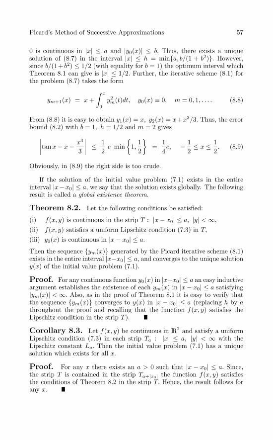
Picard’s Method of Successive Approximations 57
0 is continuous in |x| ≤ a and |y0(x)| ≤ b. Thus, there exists a uniquesolution of (8.7) in the interval |x| ≤ h = mina, b/(1 + b2). However,since b/(1+ b2) ≤ 1/2 (with equality for b = 1) the optimum interval whichTheorem 8.1 can give is |x| ≤ 1/2. Further, the iterative scheme (8.1) forthe problem (8.7) takes the form
ym+1(x) = x+∫ x
0y2
m(t)dt, y0(x) ≡ 0, m = 0, 1, . . . . (8.8)
From (8.8) it is easy to obtain y1(x) = x, y2(x) = x+x3/3. Thus, the errorbound (8.2) with b = 1, h = 1/2 and m = 2 gives
∣∣∣∣tanx− x− x3
3
∣∣∣∣ ≤ 12e min
1,
12
=
14e, − 1
2≤ x ≤ 1
2. (8.9)
Obviously, in (8.9) the right side is too crude.
If the solution of the initial value problem (7.1) exists in the entireinterval |x−x0| ≤ a, we say that the solution exists globally. The followingresult is called a global existence theorem.
Theorem 8.2. Let the following conditions be satisfied:
(i) f(x, y) is continuous in the strip T : |x− x0| ≤ a, |y| < ∞,
(ii) f(x, y) satisfies a uniform Lipschitz condition (7.3) in T,(iii) y0(x) is continuous in |x− x0| ≤ a.
Then the sequence ym(x) generated by the Picard iterative scheme (8.1)exists in the entire interval |x−x0| ≤ a, and converges to the unique solutiony(x) of the initial value problem (7.1).
Proof. For any continuous function y0(x) in |x−x0| ≤ a an easy inductiveargument establishes the existence of each ym(x) in |x− x0| ≤ a satisfying|ym(x)| < ∞. Also, as in the proof of Theorem 8.1 it is easy to verify thatthe sequence ym(x) converges to y(x) in |x − x0| ≤ a (replacing h by athroughout the proof and recalling that the function f(x, y) satisfies theLipschitz condition in the strip T ).
Corollary 8.3. Let f(x, y) be continuous in IR2 and satisfy a uniformLipschitz condition (7.3) in each strip Ta : |x| ≤ a, |y| < ∞ with theLipschitz constant La. Then the initial value problem (7.1) has a uniquesolution which exists for all x.
Proof. For any x there exists an a > 0 such that |x − x0| ≤ a. Since,the strip T is contained in the strip Ta+|x0| the function f(x, y) satisfiesthe conditions of Theorem 8.2 in the strip T. Hence, the result follows forany x.

58 Lecture 8
Problems
8.1. Compute the first few Picard’s iterates with y0(x) ≡ 0 for theinitial value problem y′ = xy + 2x − x3, y(0) = 0 and show that theyconverge to the solution y(x) = x2 for all x.
8.2. For the following initial value problems compute the first threeiterates with the initial approximation y0(x) ≡ x:
(i) y′ = x2 − y2 − 1, y(0) = 0.(ii) y′ = (x+ 2y)/(2x+ y), y(1) = 1.(iii) y′ = x2 + y2, y(0) = 0.
8.3. Discuss the existence and uniqueness of the solutions of the fol-lowing initial value problems:
(i) y′ = 1 + y2/3, y(0) = 0.(ii) y′ = sin(xy), y(0) = 1.(iii) y′ = (x+ y)x2y2, y(0) = 1.(iv) y′ = ex + x/y, y(0) = 1.
8.4. Show that the following initial value problems possess a uniquesolution for all real x:
(i) y′ + p(x)y = q(x), y(x0) = y0, where p(x) and q(x) are continuous inIR.(ii) y′ = p(x)f(cos y) + q(x)g(sin y), y(x0) = y0, where p(x) and q(x)are continuous in IR, and f and g are polynomials of degree m and n,respectively.(iii) y′ = y3ex(1 + y2)−1 + x2 cos y, y(x0) = y0.
(iv) y′ = (cosx)e−y2+ sin y, y(x0) = y0.
8.5. Show that the initial value problem
y′ = (x2 − y2) sin y + y2 cos y, y(0) = 0
has a unique solution y(x) ≡ 0 in the closed rectangle S : |x| ≤ a, |y| ≤ b.
8.6. Show that Theorem 8.1 guarantees the existence of a uniquesolution of the initial value problem y′ = e2y, y(0) = 0 in the interval(−1/2e, 1/2e). Also, solve this problem and verify that the solution existsin a larger interval.
8.7. The function f(x, y) = (tanx)y+1 is continuous in the open strip|x| < π/2, |y| < ∞. Solve the initial value problem y′ = (tanx)y + 1, y(0)= 1 and verify that the solution exists in a larger interval (−3π/2, π/2).

Picard’s Method of Successive Approximations 59
8.8. Let f1(x) and f2(y) = 0 be continuous in |x−x0| ≤ a, |y−y0| ≤ b,respectively. Show that the initial value problem y′ = f1(x)f2(y), y(x0) =y0 has a unique solution in the interval |x− x0| ≤ h where h ≤ a.
8.9. Consider the DE (3.1), where the functions M, N are continuousand having continuous partial derivatives My, Nx in the rectangle S :|x − x0| < a, |y − y0| < b (0 < a, b < ∞). Suppose that N(x, y) = 0 forall (x, y) ∈ S and the condition (3.4) holds. Show that the initial valueproblem (3.1), (1.10) has a unique solution in the interval |x − x0| ≤ hwhere h ≤ a.
8.10. If f(x, y) has continuous partial derivatives of all orders in a do-mainD, then show that themth Picard’s approximation ym(x) of the initialvalue problem (7.1) has the same value and the same derivatives up to orderm at x0 as the true solution.
8.11. Let f(x, y) be continuously p > 0 times differentiable with respectto x and y. Show that every solution of the DE (1.9) is continuously p+ 1times differentiable with respect to x.
8.12. Consider the initial value problem
y′ = f(x, y) =
y(1 − 2x), x > 0
y(2x− 1), x < 0
y(1) = 1.
(8.10)
Clearly, the function f(x, y) is discontinuous at all (0, y), y = 0. Show that
y(x) =
ex−x2
, x ≥ 0
ex2−x, x ≤ 0
is the unique continuous (but not differentiable at x = 0) solution of (8.10)which is valid for all x.
8.13. Let the conditions of Theorem 8.1 be satisfied. Show that thesuccessive approximations
ym+1(x) = y0 +(x−x0)y1 +∫ x
x0
(x− t)f(t, ym(t))dt, m = 0, 1, . . . (8.11)
with the initial approximation y0(x) = y0 converge to the unique solutionof the initial value problem (7.9) in the interval Jh : |x − x0| ≤ h =mina, b/M1, where M1 = |y1| +Ma/2.

60 Lecture 8
Answers or Hints
8.1. ym(x) = x2 − x2(m+1)/[4.6.8 · · · 2(m+ 1)].
8.2. (i) −x,−x,−x. (ii) x, x, x. (iii) 2x3/3, (x3/3)+(4x7/63), (x3/3)+(x7/63) + (8x11/2079) + (16x15/59535).
8.3. (i) Unique solution 3(y1/3 − tan−1 y1/3) = x. (ii) Global uniquesolution. (iii) Local unique solution. (iv) Local unique solution.
8.4. Apply Corollary 8.3.
8.5. The function (x2 − y2) sin y+ y2 cos y satisfies the Lipschitz condition(7.3) for all (x, y) ∈ S.
8.6. The solution y(x) = ln 1/√
(1 − 2x) exists for all x ∈ [−1/2, 1/2].
8.7. The solution y(x) = tan[(x/2) + (π/4)] exists in the interval (−3π/2,π/2).
8.8. The function G(y) =∫ y
y0dt/f2(t) =
∫ x
x0f1(s)ds exists and it is con-
tinuous and monotonic as long as |y − y0| ≤ b.
8.9. From (3.3), u(x, y) = u(x0, y0). Now use implicit function theorem.
8.10. y0(x0) = y0 = y(x0), y′1(x) = f(x, y0(x)), y′
1(x0) = f(x0, y0(x0)) =f(x0, y0) = y′(x0), y′′
2 (x0) = ∂f∂x (x0, y1(x0)) + ∂f
∂y (x0, y1(x0))y′1(x0) =
y′′(x0).
8.11. Use y′(x) = f(x, y(x)).
8.12. Verify directly.
8.13. The proof is similar to that of Theorem 8.1.

Lecture 9Existence Theorems
As promised in Lecture 7, here we shall prove that the continuity ofthe function f(x, y) alone is sufficient for the existence of a solution of theinitial value problem (7.1).
Theorem 9.1 (Peano’s Existence Theorem). Let f(x, y) becontinuous and bounded in the strip T : |x− x0| ≤ a, |y| < ∞. Then theinitial value problem (7.1) has at least one solution in |x− x0| ≤ a.
Proof. We shall give the existence proof in the interval [x0, x+ a], andits extension to [x0 −a, x0] is immediate. We define a sequence of functionsym(x) by the scheme
ym(x) = y0, x0 ≤ x ≤ x0 +a
m
ym(x) = y0 +∫ x−(a/m)
x0
f(t, ym(t))dt, x0 + ka
m≤ x ≤ x0 + (k + 1)
a
m,
k = 1, 2, . . . ,m− 1.(9.1)
The first equation defines ym(x) in [x0, x0 + a/m]; then the second equa-tion defines ym(x) at first in [x0 + a/m, x0 + 2a/m] and then in [x0 +2a/m, x0 + 3a/m] and so on. Since f(x, y) is bounded in T, we can assumethat |f(x, y)| ≤ M for all (x, y) ∈ T. Now for any two points x1, x2 in[x0, x0 + a], we have
|ym(x2) − ym(x1)|= 0 if x1, x2 ∈
[x0, x0 +
a
m
]
=
∣∣∣∣∣∫ x2−(a/m)
x0
f(t, ym(t))dt
∣∣∣∣∣ ≤ M∣∣∣x2 − a
m− x0
∣∣∣ ≤ M |x2 − x1|
if x1 ∈[x0, x0 +
a
m
], x2 ∈
[x0 + k
a
m, x0 + (k + 1)
a
m
]
=
∣∣∣∣∣∫ x2−(a/m)
x1−(a/m)f(t, ym(t))dt
∣∣∣∣∣ ≤ M |x2 − x1| otherwise.
Thus, it follows that
|ym(x2) − ym(x1)| ≤ M |x2 − x1|, x1, x2 ∈ [x0, x0 + a].
R.P. Agarwal and D. O’Regan, An Introduction to Ordinary Differential Equations,
61doi: 10.1007/978-0-387-71276-5_9, © Springer Science + Business Media, LLC 2008

62 Lecture 9
Hence, |ym(x2) − ym(x1)| ≤ ε provided |x2 − x1| ≤ ε/M = δ; i.e., thesequence ym(x) is equicontinuous. Moreover, for all x ∈ [x0, x0 + a],we have
|ym(x)| ≤ |y0| +M∣∣∣x− a
m− x0
∣∣∣ ≤ |y0| +Ma,
i.e., the sequence ym(x) is uniformly bounded in [x0, x0 + a]. Therefore,from Theorem 7.10 the sequence ym(x) contains a subsequence ymp(x)which converges uniformly in [x0, x0 + a] to a continuous function y(x). Toshow that the function y(x) is a solution of the initial value problem (7.1),we let p → ∞ in the relation
ymp(x) = y0 +∫ x
x0
f(t, ymp(t))dt−∫ x
x−(a/mp)f(t, ymp
(t))dt.
Since f(x, y) is continuous and the convergence is uniform, in the first inte-gral we can take the limit inside the integral sign to obtain
∫ x
x0f(t, y(t))dt.
The second integral does not exceed M(a/mp) and hence tends to zero.Thus, y(x) is a solution of the integral equation (7.2).
Corollary 9.2. Let f(x, y) be continuous in S, and hence there existsa M > 0 such that |f(x, y)| ≤ M for all (x, y) ∈ S. Then the initial valueproblem (7.1) has at least one solution in Jh.
Proof. The proof is the same as that of Theorem 9.1 with some obviouschanges.
Example 9.1. The function f(x, y) = y2/3 is continuous for all (x, y) inIR2. Thus, from Corollary 9.2 the initial value problem y′ = y2/3, y(0) = 0has at least one solution in the interval |x| ≤ h = mina, b1/3. However,we can choose b sufficiently large so that h = a. Hence, the given problemin fact has at least one solution for all x in IR.
Next for a given continuous function f(x, y) in a domain D, we needthe following definition.
Definition 9.1. A function y(x) defined in J is said to be an ε-approximate solution of the DE y′ = f(x, y) if (i) y(x) is continuous for allx in J, (ii) for all x ∈ J the points (x, y(x)) ∈ D, (iii) y(x) has a piecewisecontinuous derivative in J which may fail to be defined only for a finitenumber of points, say, x1, x2, . . . , xk, and (iv) |y′(x) − f(x, y(x))| ≤ ε forall x ∈ J, x = xi, i = 1, 2, . . . , k.
The existence of an ε-approximate solution is proved in the followingtheorem.
Theorem 9.3. Let f(x, y) be continuous in S and hence there exists aM > 0 such that |f(x, y)| ≤ M for all (x, y) ∈ S. Then for any ε > 0, there

Existence Theorems 63
exists an ε-approximate solution y(x) of the DE y′ = f(x, y) in the intervalJh such that y(x0) = y0.
Proof. Since f(x, y) is continuous in the closed rectangle S, it is uni-formly continuous in this rectangle. Thus, for a given ε > 0 there exists aδ > 0 such that
|f(x, y) − f(x1, y1)| ≤ ε (9.2)
for all (x, y), (x1, y1) in S whenever |x− x1| ≤ δ and |y − y1| ≤ δ.
We shall construct an ε-approximate solution in the interval x0 ≤ x ≤x0 + h and a similar process will define it in the interval x0 − h ≤ x ≤ x0.For this, we divide the interval x0 ≤ x ≤ x0 + h into m parts x0 < x1 <· · · < xm = x0 + h such that
xi − xi−1 ≤ minδ,δ
M
, i = 1, 2, . . . ,m. (9.3)
Next we define a function y(x) in the interval x0 ≤ x ≤ x0 + h by therecursive formula
y(x) = y(xi−1)+(x−xi−1)f(xi−1, y(xi−1)), xi−1 ≤ x ≤ xi, i = 1, 2, . . . ,m.(9.4)
Obviously, this function y(x) is continuous and has a piecewise contin-uous derivative y′(x) = f(xi−1, y(xi−1)), xi−1 < x < xi, i = 1, 2, . . . ,mwhich fails to be defined only at the points xi, i = 1, 2, . . . ,m − 1. Sincein each subinterval [xi−1, xi], i = 1, 2, . . . ,m the function y(x) is a straightline, to prove (x, y(x)) ∈ S it suffices to show that |y(xi) − y0| ≤ b for alli = 1, 2, . . . ,m. For this, in (9.4) let i = 1 and x = x1 to obtain
|y(x1) − y0| = (x1 − x0)|f(x0, y0)| ≤ Mh ≤ b.
Now let the assertion be true for i = 1, 2, . . . , k − 1 < m − 1, then from(9.4), we find
y(x1) − y0 = (x1 − x0)f(x0, y0)y(x2) − y(x1) = (x2 − x1)f(x1, y(x1))
· · ·y(xk) − y(xk−1) = (xk − xk−1)f(xk−1, y(xk−1))
and hence,
y(xk) − y0 =k∑
=1
(x − x−1)f(x−1, y(x−1)),
which gives
|y(xk) − y0| ≤k∑
=1
(x − x−1)M = M(xk − x0) ≤ Mh ≤ b.

64 Lecture 9
Finally, if xi−1 < x < xi then from (9.4) and (9.3), we have
|y(x) − y(xi−1)| ≤ M |x− xi−1| ≤ Mδ
M= δ
and hence from (9.2), we find
|y′(x) − f(x, y(x))| = |f(xi−1, y(xi−1)) − f(x, y(x))| ≤ ε
for all x ∈ Jh, x = xi, i = 1, 2, . . . ,m−1. This completes the proof that y(x)is an ε-approximate solution of the DE y′ = f(x, y). This method of con-structing an approximate solution is known as Cauchy–Euler method.
Now we restate Corollary 9.2, and prove it as a consequence of Theo-rem 9.3.
Theorem 9.4 (Cauchy–Peano’s Existence Theorem). Letthe conditions of Theorem 9.3 be satisfied. Then the initial value problem(7.1) has at least one solution in Jh.
Proof. Once again we shall give the proof only in the interval x0 ≤x ≤ x0 + h. Let εm be a monotonically decreasing sequence of positivenumbers such that εm → 0. For each εm we use Theorem 9.3 to construct anε-approximate solution ym(x). Now as in Theorem 9.1, for any two pointsx and x∗ in [x0, x0 + h] it is easy to prove that
|ym(x) − ym(x∗)| ≤ M |x− x∗|
and from this it follows that the sequence ym(x) is equicontinuous. Fur-ther, as in Theorem 9.3 for each x in [x0, x0 +h], we have |ym(x)| ≤ |y0|+b,and hence the sequence ym(x) is also uniformly bounded. Therefore,again Theorem 7.10 is applicable and the sequence ym(x) contains a sub-sequence ymp
(x) which converges uniformly in [x0, x0+h] to a continuousfunction y(x). To show that the function y(x) is a solution of (7.1), we define
em(x) = y′m(x) − f(x, ym(x)), at the points where y′
m(x) exists
= 0, otherwise.
Thus, it follows that
ym(x) = y0 +∫ x
x0
[f(t, ym(t)) + em(t)]dt (9.5)
and |em(x)| ≤ εm. Since f(x, y) is continuous in S and ymp(x) convergesto y(x) uniformly in [x0, x0 + h], the function f(x, ymp(x)) converges tof(x, y(x)) uniformly in [x0, x0 + h]. Further, since εmp → 0 we find that|εmp(x)| converges to zero uniformly in [x0, x0 + h]. Thus, by replacing m

Existence Theorems 65
by mp in (9.5) and letting p → ∞, we find that y(x) is a solution of theintegral equation (7.2).
Corollary 9.2 essentially states the following: If in a domain D thefunction f(x, y) is continuous, then for every point (x0, y0) in D there isa rectangle S such that (7.1) has a solution y(x) in Jh. Since S lies in D,by applying Corollary 9.2 to the point at which the solution goes out of S,we can extend the region in which the solution exists. For example, thefunction y(x) = 1/(1 − x) is the solution of the problem y′ = y2, y(0) = 1.Clearly, this solution exists in (−∞, 1). For this problem
S : |x| ≤ a, |y − 1| ≤ b, M = maxS
y2 = (1 + b)2
and h = mina, b/(1 + b)2. Since b/(1 + b)2 ≤ 1/4 we can (independent ofthe choice of a) take h = 1/4. Thus, Corollary 9.2 gives the existence of asolution y1(x) only in the interval |x| ≤ 1/4. Now consider the continuationof y1(x) to the right obtained by finding a solution y2(x) of the problemy′ = y2, y(1/4) = 4/3. For this new problem S : |x−1/4| ≤ a, |y−4/3| ≤ b,and maxS y
2 = (4/3+ b)2. Since b/(4/3+ b)2 ≤ 3/16 we can take h = 3/16.Thus, y2(x) exists in the interval |x−1/4| ≤ 3/16. This ensures the existenceof a solution
y(x) =
y1(x), − 1/4 ≤ x ≤ 1/4
y2(x), 1/4 ≤ x ≤ 7/10
in the interval −1/4 ≤ x ≤ 7/16. This process of continuation of the solutioncan be used further to the right of the point (7/16, 16/9), or to the left ofthe point (−1/4, 4/5). In order to establish how far the solution can becontinued, we need the following lemma.
Lemma 9.5. Let f(x, y) be continuous in the domain D and letsupD |f(x, y)| ≤ M. Further, let the initial value problem (7.1) has a solu-tion y(x) in an interval J = (α, β). Then the limits limx→α+ y(x) = y(α+0)and limx→β− y(x) = y(β − 0) exist.
Proof. For α < x1 < x2 < β, integral equation (7.2) gives that
|y(x2) − y(x1)| ≤∫ x2
x1
|f(t, y(t))|dt ≤ M |x2 − x1|.
Therefore, y(x2) − y(x1) → 0 as x1, x2 → α+. Thus, by the Cauchy cri-terion of convergence limx→α+ y(x) exists. A similar argument holds forlimx→β− y(x).
Theorem 9.6. Let the conditions of Lemma 9.5 be satisfied and let(β, y(β − 0)) ∈ D ((α, y(α+ 0)) ∈ D). Then the solution y(x) of the initialvalue problem (7.1) in (α, β) can be extended over the interval (α, β +γ] ([α− γ, β)) for some γ > 0.

66 Lecture 9
Proof. We define the function y1(x) as follows: y1(x) = y(x) for x ∈(α, β) and y1(β) = y(β − 0). Then since for all x ∈ (α, β]
y1(x) = y(β − 0) +∫ x
β
f(t, y1(t))dt
= y0 +∫ β
x0
f(t, y1(t))dt+∫ x
β
f(t, y1(t))dt
= y0 +∫ x
x0
f(t, y1(t))dt,
the left-hand derivative y′1(β− 0) exists and y′
1(β− 0) = f(β, y1(β)). Thus,y1(x) is a continuation of y(x) in the interval (α, β]. Next let y2(x) be asolution of the problem y′ = f(x, y), y(β) = y1(β) existing in the interval[β, β + γ], then the function
y3(x) =y1(x), x ∈ (α, β]y2(x), x ∈ [β, β + γ]
is a continuation of y(x) in the interval (α, β + γ]. For this, it suffices tonote that
y3(x) = y0 +∫ x
x0
f(t, y3(t))dt (9.6)
for all x ∈ (α, β + γ]. In fact (9.6) is obvious for all x ∈ (α, β] from thedefinition of y3(x) and for x ∈ [β, β + γ], we have
y3(x) = y(β − 0) +∫ x
β
f(t, y3(t))dt
= y0 +∫ β
x0
f(t, y3(t))dt+∫ x
β
f(t, y3(t))dt
= y0 +∫ x
x0
f(t, y3(t))dt.
Problems
9.1. Let f(x, y) be continuous and |f(x, y)| ≤ c1 +c2|y|α for all (x, y) ∈T : |x − x0| ≤ a, |y| < ∞ where c1 and c2 are nonnegative constantsand 0 ≤ α < 1. Show that the initial value problem (7.1) has at least onesolution in the interval |x− x0| ≤ a.
9.2. Let f(x, y) be continuous and satisfy the Lipschitz condition (7.3)in a domain D. Further, let yi(x), i = 1, 2 be εi-approximate solutions ofthe DE y′ = f(x, y) in J and x0 ∈ J. Show that for all x ∈ J
|y1(x) − y2(x)| ≤(
|y1(x0) − y2(x0)| +ε1 + ε2L
)exp(L|x− x0|) − ε1 + ε2
L.

Existence Theorems 67
9.3. Show that the solution of the problem y′ = −x/y, y(0) = 1 cannotbe extended beyond the interval −1 < x < 1.
9.4. Show that the solution of the problem y′ = y2, y(0) = 2 is ex-tendable only to the interval −∞ < x < 1/2.
9.5. Show that the solution of the problem y′ = 2xy2, y(0) = 1 existsonly in the interval |x| < 1.
9.6. Show that the solution of the problem y′ = 1+y2, y(0) = 1 cannotbe extended beyond the interval −3π/4 < x < π/4.
9.7. Find the maximum interval in which the solution of the problemy′ + (sinx)y2 = 3(xy)2, y(0) = 2 can be extended.
9.8. Find the maximum interval of existence of solutions of y′ +3y4/3 sinx = 0 satisfying (i) y(π/2) = 0, (ii) y(π/2) = 1/8, and (iii) y(π/2)= 8.
9.9. Solve the initial value problem
yy′ − 3x2(1 + y2) = 0, y(0) = 1.
Find also the largest interval on which the solution is defined.
Answers or Hints
9.1. In the rectangle S : |x−x0| ≤ a, |y−y0| ≤ b, |f(x, y)| ≤ c1 +c2(|y0|+b)α = K. Note that b/K → ∞ as b → ∞.
9.2. For x ≥ x0, |y′i(x) − f(x, yi(x))| ≤ εi, i = 1, 2 yields |yi(x) − yi(x0) −∫ x
x0f(t, yi(t))dt| ≤ εi(x− x0). Now use |p− q| ≤ |p| + |q| and Corollary 7.6.
9.3. Although the solution y(x) =√
1 − x2 is defined on [−1, 1] its deriva-tive is not defined at x = ±1.
9.4. The solution is y(x) = 2/(1 − 2x).
9.5. The solution is y(x) = 1/(1 − x2).
9.6. The solution is y(x) = tan(x+ π/4).
9.7. The solution is y(x) = 1/[(3/2) − cosx − x3], which is defined in(−∞, 0.9808696 · · ·).9.8. (i) The solution is y(x) ≡ 0, which is defined on IR. (ii) The solutionis y(x) = 1/(2− cosx)3, which is defined on IR. (iii) The solution is y(x) =1/[(1/2) − cosx]3, which is defined in (π/3, 5π/3).
9.9. y =(2e2x3 − 1
)1/2, x >
( 12 ln 1
2
)1/3.

Lecture 10Uniqueness Theorems
In our previous lectures we have proved that the continuity of the func-tion f(x, y) in the closed rectangle S is sufficient for the existence of atleast one solution of the initial value problem (7.1) in the interval Jh, andto achieve the uniqueness (i.e., existence of at most one solution) someadditional condition on f(x, y) is required. In fact, continuous functionsf(x, y) have been constructed (see Lavrentev [30], Hartman [20]) so thatfrom any given point (x0, y0) the equation y′ = f(x, y) has at least twosolutions in every neighborhood of (x0, y0). In Theorem 8.1 this additionalcondition was assumed to be the Lipschitz continuity. In the following, weshall provide several such conditions which are sufficient for the uniquenessof the solutions of (7.1).
Theorem 10.1 (Lipschitz Uniqueness Theorem). Letf(x, y) be continuous and satisfy a uniform Lipschitz condition (7.3) in S.Then (7.1) has at most one solution in |x− x0| ≤ a.
Proof. In Theorem 8.1 the uniqueness of the solutions of (7.1) is provedin the interval Jh; however, it is clear that Jh can be replaced by the interval|x− x0| ≤ a.
Theorem 10.2 (Peano’s Uniqueness Theorem). Let f(x, y)be continuous in S+ : x0 ≤ x ≤ x0 + a, |y − y0| ≤ b and nonincreasing iny for each fixed x in x0 ≤ x ≤ x0 + a. Then (7.1) has at most one solutionin x0 ≤ x ≤ x0 + a.
Proof. Suppose y1(x) and y2(x) are two solutions of (7.1) in x0 ≤x ≤ x0 + a which differ somewhere in x0 ≤ x ≤ x0 + a. We assume thaty2(x) > y1(x) in x1 < x < x1 + ε ≤ x0 + a, while y1(x) = y2(x) inx0 ≤ x ≤ x1, i.e., x1 is the greatest lower bound of the set A consisting ofthose x for which y2(x) > y1(x). This greatest lower bound exists becausethe set A is bounded below by x0 at least. Thus, for all x ∈ (x1, x1 + ε)we have f(x, y1(x)) ≥ f(x, y2(x)); i.e., y′
1(x) ≥ y′2(x). Hence, the function
z(x) = y2(x) − y1(x) is nonincreasing, since if z(x1) = 0 we should havez(x) ≤ 0 in (x1, x1 + ε). This contradiction proves that y1(x) = y2(x) inx0 ≤ x ≤ x0 + a.
Example 10.1. The function |y|1/2sgn y, where sgn y = 1 if y ≥ 0,and −1 if y < 0 is continuous, nondecreasing, and the initial value problemy′ = |y|1/2sgn y, y(0) = 0 has two solutions y(x) ≡ 0, y(x) = x2/4 in the
R.P. Agarwal and D. O’Regan, An Introduction to Ordinary Differential Equations,
68doi: 10.1007/978-0-387-71276-5_10, © Springer Science + Business Media, LLC 2008

Uniqueness Theorems 69
interval [0,∞). Thus, in Theorem 10.2 “nonincreasing” cannot be replacedby “nondecreasing.”
For our next result, we need the following lemma.
Lemma 10.3. Let w(z) be continuous and increasing function in theinterval [0,∞), and w(0) = 0, w(z) > 0 for z > 0, with also
limε→0+
∫ε
dz
w(z)= ∞. (10.1)
Let u(x) be a nonnegative continuous function in [0, a]. Then the inequality
u(x) ≤∫ x
0w(u(t))dt, 0 < x ≤ a (10.2)
implies that u(x) ≡ 0 in [0, a].
Proof. Define v(x) = max0≤t≤x u(t) and assume that v(x) > 0 for0 < x ≤ a. Then u(x) ≤ v(x) and for each x there is an x1 ≤ x such thatu(x1) = v(x). From this, we have
v(x) = u(x1) ≤∫ x1
0w(u(t))dt ≤
∫ x
0w(v(t))dt;
i.e., the nondecreasing function v(x) satisfies the same inequality as u(x)does. Let us set
v(x) =∫ x
0w(v(t))dt,
then v(0) = 0, v(x) ≤ v(x), v′(x) = w(v(x)) ≤ w(v(x)). Hence, for 0 <δ < a, we have ∫ a
δ
v′(x)w(v(x))
dx ≤ a− δ < a.
However, from (10.1) it follows that∫ a
δ
v′(x)w(v(x))
dx =∫ α
ε
dz
w(z), v(δ) = ε, v(a) = α
becomes infinite when ε → 0 (δ → 0). This contradiction shows that v(x)cannot be positive, so v(x) ≡ 0, and hence u(x) = 0 in [0, a].
Theorem 10.4 (Osgood’s Uniqueness Theorem). Letf(x, y) be continuous in S and for all (x, y1), (x, y2) ∈ S it satisfies
|f(x, y1) − f(x, y2)| ≤ w(|y1 − y2|), (10.3)
where w(z) is the same as in Lemma 10.3. Then (7.1) has at most onesolution in |x− x0| ≤ a.

70 Lecture 10
Proof. Suppose y1(x) and y2(x) are two solutions of (7.1) in |x−x0| ≤ a.Then from (10.3) it follows that
|y1(x) − y2(x)| ≤∣∣∣∣∫ x
x0
w(|y1(t) − y2(t)|)dt∣∣∣∣ .
For any x in [x0, x0 + a], we set u(x) = |y1(x0 + x) − y2(x0 + x)|. Then thenonnegative continuous function u(x) satisfies the inequality (10.2), andtherefore, Lemma 10.3 implies that u(x) = 0 in [0, a], i.e., y1(x) = y2(x) in[x0, x0+a]. If x is in [x0−a, x0], then the proof remains the same except thatwe need to define the function u(x) = |y1(x0−x)−y2(x0−x)| in [0, a].
For our next result, we shall prove the following lemma.
Lemma 10.5. Let u(x) be nonnegative continuous function in |x−x0| ≤a, and u(x0) = 0, and let u(x) be differentiable at x = x0 with u′(x0) = 0.Then the inequality
u(x) ≤∣∣∣∣∫ x
x0
u(t)t− x0
dt
∣∣∣∣ (10.4)
implies that u(x) = 0 in |x− x0| ≤ a.
Proof. It suffices to prove the lemma only for x0 ≤ x ≤ x0 + a. Wedefine
v(x) =∫ x
x0
u(t)t− x0
dt.
This integral exists since
limx→x0
u(x)x− x0
= u′(x0) = 0.
Further, we have
v′(x) =u(x)x− x0
≤ v(x)x− x0
and hence d/dx[v(x)/(x − x0)] ≤ 0, which implies that v(x)/(x − x0) isnonincreasing. Since v(x0) = 0, this gives v(x) ≤ 0, which is a contradictionto v(x) ≥ 0. So, v(x) ≡ 0, and hence u(x) = 0 in [x0, x0 + a].
Theorem 10.6 (Nagumo’s Uniqueness Theorem). Letf(x, y) be continuous in S and for all (x, y1), (x, y2) ∈ S it satisfies
|f(x, y1) − f(x, y2)| ≤ k|x− x0|−1|y1 − y2|, x = x0, k ≤ 1. (10.5)
Then (7.1) has at most one solution in |x− x0| ≤ a.
Proof. Suppose y1(x) and y2(x) are two solutions of (7.1) in |x−x0| ≤ a.Then from (10.5) it follows that
|y1(x) − y2(x)| ≤∣∣∣∣∫ x
x0
|t− x0|−1|y1(t) − y2(t)|dt∣∣∣∣ .

Uniqueness Theorems 71
We set u(x) = |y1(x) − y2(x)|; then the nonnegative function u(x) satisfiesthe inequality (10.4). Further, since u(x) is continuous in |x−x0| ≤ a, andu(x0) = 0, from the mean value theorem we have
u′(x0) = limh→0
u(x0 + h) − u(x0)h
= limh→0
|y1(x0) + hy′1(x0 + θ1h) − y2(x0) − hy′
2(x0 + θ2h)|h
,
0 < θ1, θ2 < 1
= (sgn h) limh→0
|y′1(x0 + θ1h) − y′
2(x0 + θ2h)| = 0.
Thus, the conditions of Lemma 10.5 are satisfied and u(x) ≡ 0, i.e., y1(x) =y2(x) in |x− x0| ≤ a.
Example 10.2. It is easy to verify that the function
f(x, y) =
⎧⎪⎪⎨⎪⎪⎩
0 0 ≤ x ≤ 1, y ≤ 0(1 + ε)y
x0 ≤ x ≤ 1, 0 < y < x1+ε, ε > 0
(1 + ε)xε 0 ≤ x ≤ 1, x1+ε ≤ y
is continuous and satisfies the condition (10.5) (except k = 1 + ε > 1)in S : [0, 1] × IR. For this function the initial value problem (7.1) with(x0, y0) = (0, 0) has an infinite number of solutions y(x) = cx1+ε, where cis an arbitrary constant such that 0 < c < 1. Thus, in condition (10.5) theconstant k ≤ 1 is the best possible, i.e., it cannot be replaced by k > 1.
Theorem 10.7 (Krasnoselski–Krein Uniqueness Theo-rem). Let f(x, y) be continuous in S and for all (x, y1), (x, y2) ∈ S itsatisfies
|f(x, y1) − f(x, y2)| ≤ k|x− x0|−1|y1 − y2|, x = x0, k > 0 (10.6)
|f(x, y1) − f(x, y2)| ≤ C|y1 − y2|α, C > 0, 0 < α < 1, k(1 − α) < 1.(10.7)
Then (7.1) has at most one solution in |x− x0| ≤ a.
Proof. Suppose y1(x) and y2(x) are two solutions of (7.1) in |x−x0| ≤ a.We shall show that y1(x) = y2(x) only in the interval [x0, x0 + a]. For this,from (10.7) we have
u(x) = |y1(x) − y2(x)| ≤∫ x
x0
Cuα(t)dt
and hence Problem 7.5 gives that
u(x) ≤ [C(1 − α)(x− x0)](1−α)−1 ≤ [C(x− x0)](1−α)−1.

72 Lecture 10
Thus, the function v(x) = u(x)/(x− x0)k satisfies the inequality
0 ≤ v(x) ≤ C(1−α)−1(x− x0)(1−α)−1−k. (10.8)
Since k(1−α) < 1, it is immediate that limx→x0 v(x) = 0.Hence, if we definev(x0) = 0, then the function v(x) is continuous in [x0, x0 + a]. We wish toshow that v(x) = 0 in [x0, x0+a]. If v(x) > 0 at any point in [x0, x0+a], thenthere exists a point x1 > x0 such that 0 < m = v(x1) = maxx0≤x≤x0+a v(x).However, from (10.6) we obtain
m = v(x1) ≤ (x1 − x0)−k
∫ x1
x0
k(t− x0)−1u(t)dt
≤ (x1 − x0)−k
∫ x1
x0
k(t− x0)k−1v(t)dt
< m(x1 − x0)−k
∫ x1
x0
k(t− x0)k−1dt
= m(x1 − x0)−k(x1 − x0)k = m,
which is the desired contradiction. So, v(x) ≡ 0, and hence u(x) = 0 in[x0, x0 + a].
Theorem 10.8 (Van Kampen Uniqueness Theorem). Letf(x, y) be continuous in S and for all (x, y) ∈ S it satisfies
|f(x, y)| ≤ A|x− x0|p, p > −1, A > 0. (10.9)
Further, let for all (x, y1), (x, y2) ∈ S it satisfies
|f(x, y1) − f(x, y2)| ≤ C
|x− x0|r |y1 − y2|q, q ≥ 1, C > 0 (10.10)
with q(1 + p) − r = p, ρ = C(2A)q−1/(p+ 1)q < 1. Then (7.1) has at mostone solution in |x− x0| ≤ a.
Proof. Suppose y1(x) and y2(x) are two solutions of (7.1) in |x−x0| ≤ a.We shall show that y1(x) = y2(x) only in the interval [x0 − a, x0]. For this,from (10.9) we have
u(x) = |y1(x) − y2(x)| ≤∫ x0
x
|f(t, y1(t)) − f(t, y2(t))|dt
≤ 2A∫ x0
x
(x0 − t)pdt =2Ap+ 1
(x0 − x)p+1.
Using this estimate and (10.10), we obtain
u(x) ≤ C
∫ x0
x
1(x0 − t)r
uq(t)dt
≤ C
(2Ap+ 1
)q ∫ x0
x
(x0 − t)q(p+1)−rdt = ρ
(2Ap+ 1
)(x0 − x)p+1.

Uniqueness Theorems 73
Now using this new estimate and (10.10), we get
u(x) ≤ ρ1+q
(2Ap+ 1
)(x0 − x)p+1.
Continuing in this way, we find
u(x) ≤ ρ1+q+q2+···+qm
(2Ap+ 1
)(x0 − x)p+1, m = 1, 2, . . . .
Since q ≥ 1 and ρ < 1, it follows that u(x) = 0 in |x0 − a, x0].
Problems
10.1. Consider the initial value problem
y′ = f(x, y) =
⎧⎨⎩
4x3y
x4 + y2 , (x, y) = (0, 0)
0, (x, y) = (0, 0)
y(0) = 0.
(10.11)
Show that the function f(x, y) is continuous but does not satisfy the Lips-chitz condition in any region containing the origin (see Problem 7.4). Fur-ther, show that (10.11) has an infinite number of solutions.
10.2. Given the equation y′ = xg(x, y), suppose that g and ∂g/∂y aredefined and continuous for all (x, y). Show the following:
(i) y(x) ≡ 0 is a solution.(ii) If y = y(x), x ∈ (α, β) is a solution and if y(x0) > 0, x0 ∈ (α, β),then y(x) > 0 for all x ∈ (α, β).(iii) If y = y(x), x ∈ (α, β) is a solution and if y(x0) < 0, x0 ∈ (α, β),then y(x) < 0 for all x ∈ (α, β).
10.3. Let f(x, y) be continuous and satisfy the generalized Lipschitzcondition
|f(x, y1) − f(x, y2)| ≤ L(x)|y1 − y2|for all (x, y1), (x, y2) in S, where the function L(x) is such that the integral∫ x0+a
x0−aL(t)dt exists. Show that (7.1) has at most one solution in |x−x0| ≤ a.
10.4. Give some examples to show that the Lipschitz condition inTheorem 10.1 is just a sufficient condition for proving the uniqueness of thesolutions of (7.1) but not the necessary condition.

74 Lecture 10
10.5. Let f(x, y) be continuous in S+ and for all (x, y1), (x, y2) in S+with y2 ≥ y1 satisfy one sided Lipschitz condition
f(x, y2) − f(x, y1) ≤ L(y2 − y1).
Show that (7.1) has at most one solution in x0 ≤ x ≤ x0 + a.
10.6. Let f(x, y) be continuous in S− : x0 − a ≤ x ≤ x0, |y − y0| ≤ band nondecreasing in y for each fixed x in x0 −a ≤ x ≤ x0. Show that (7.1)has at most one solution in x0 − a ≤ x ≤ x0.
10.7. Show that the functions w(z) = Lzα (α ≥ 1), and
w(z) =
−z ln z, 0 ≤ z ≤ e−1
e−1, z > e−1
satisfy the conditions of Lemma 10.3.
10.8. Consider the function f(x, y) in the strip T : − ∞ < x ≤ 1,−∞ < y < ∞ defined by
f(x, y) =
⎧⎪⎪⎪⎪⎨⎪⎪⎪⎪⎩
0 −∞ < x ≤ 0, − ∞ < y < ∞2x 0 < x ≤ 1, − ∞ < y < 0
2x− 4yx
0 < x ≤ 1, 0 ≤ y ≤ x2
−2x 0 < x ≤ 1, x2 < y < ∞.
Show that the problem y′ = f(x, y), y(0) = 0 has a unique solution in theinterval −∞ < x ≤ 1. Further, show that the Picard iterates with y0(x) ≡ 0for this problem do not converge.
10.9. Consider the function f(x, y) in the strip T : 0 ≤ x ≤ 1, −∞ <y < ∞ defined by
f(x, y) =
⎧⎪⎪⎨⎪⎪⎩
0 0 ≤ x ≤ 1, x1/(1−α) < y < ∞, 0 < α < 1
kxα/(1−α) − ky
x0 ≤ x ≤ 1, 0 ≤ y ≤ x1/(1−α), k > 0
kxα/(1−α) 0 ≤ x ≤ 1, − ∞ < y < 0, k(1 − α) < 1.
Show that the problem y′ = f(x, y), y(0) = 0 has a unique solution in [0, 1].
∗10.10 (Rogers’ Uniqueness Theorem). Let f(x, y) be continuousin the strip T : 0 ≤ x ≤ 1, − ∞ < y < ∞ and satisfy the condition
f(x, y) = o(e−1/xx−2
)uniformly for 0 ≤ y ≤ δ, δ > 0 arbitrary. Further, let for all (x, y1), (x, y2)∈ T it satisfy
|f(x, y1) − f(x, y2)| ≤ 1x2 |y1 − y2|.

Uniqueness Theorems 75
Show that the problem y′ = f(x, y), y(0) = 0 has at most one solution in[0, 1].
10.11. Consider the function f(x, y) in the strip T : 0 ≤ x ≤ 1, −∞ <y < ∞ defined by
f(x, y) =
⎧⎪⎪⎪⎪⎨⎪⎪⎪⎪⎩
(1 +
1x
)e−1/x 0 ≤ x ≤ 1, xe−1/x ≤ y < ∞
y
x2 + e−1/x 0 ≤ x ≤ 1, 0 ≤ y ≤ xe−1/x
e−1/x 0 ≤ x ≤ 1, − ∞ < y ≤ 0.
Show that the problem y′ = f(x, y), y(0) = 0 has a unique solution in [0, 1].
10.12. Consider the function f(x, y) in the strip T : 0 ≤ x ≤ 1, −∞ <y < ∞ defined by
f(x, y) =
⎧⎪⎪⎪⎪⎨⎪⎪⎪⎪⎩
0 0 ≤ x ≤ 1, − ∞ < y ≤ 0y
x2 0 ≤ x ≤ 1, 0 ≤ y ≤ e−1/x
e−1/x
x2 0 ≤ x ≤ 1, e−1/x ≤ y < ∞.
Show that the problem y′ = f(x, y), y(0) = 0 has an infinite number ofsolutions in [0, 1].
Answers or Hints
10.1. y = c2 − √x4 + c4, where c is arbitrary.
10.2. (i) Verify directly. (ii) Use Theorem 10.1. (iii) Use Theorem 10.1.
10.3. Since∫ x0+a
x0−aL(t)dt exists, Corollary 7.4 is applicable.
10.4. Consider the Problem 8.3(i), or y′ = y ln(1/y), y(0) = α ≥ 0.
10.5. Suppose two solutions y1(x) and y2(x) are such that y2(x) > y1(x),x1 < x < x1 + ε ≤ x0 + a and y1(x) = y2(x), x0 ≤ x ≤ x1. Now applyCorollary 7.4.
10.6. The proof is similar to that of Theorem 10.2.
10.7. Verify directly.
10.8. The given function is continuous and bounded by 2 in T. Also itsatisfies the conditions of Theorem 10.2 (also, see Problem 10.6). The only
solution is y(x) =
0, − ∞ < x ≤ 0x2/3, 0 < x ≤ 1. The successive approximations are
y2m−1(x) = x2, y2m(x) = −x2, m = 1, 2, . . . .

76 Lecture 10
10.9. Show that conditions of Theorem 10.7 are satisfied. The only solutionis y(x) = k(1 − α)x1/(1−α)/[k(1 − α) + 1].
10.11. Show that conditions of Problem 10.10 are satisfied. The only so-lution is y(x) = xe−1/x.
10.12. Show that the condition f(x, y) = o(e−1/xx−2
)of Problem 10.10 is
not satisfied. For each 0 ≤ c ≤ 1, y(x) = ce−1/x is a solution.

Lecture 11Differential Inequalities
Let the function f(x, y) be continuous in a given domain D. A functiony(x) is said to be a solution of the differential inequality y′ > f(x, y) inJ = [x0, x0 + a) if (i) y′(x) exists for all x ∈ J, (ii) for all x ∈ J the points(x, y(x)) ∈ D, and (iii) y′(x) > f(x, y(x)) for all x ∈ J. The solutions ofthe differential inequalities y′ ≥ f(x, y), y′ < f(x, y), and y′ ≤ f(x, y)are defined analogously. For example, y(x) = cotx is a solution of thedifferential inequality y′ < −y2 in the interval (0, π).
Our first basic result for differential inequalities is stated in the followingtheorem.
Theorem 11.1. Let f(x, y) be continuous in the domain D and y1(x)and y2(x) be the solutions of the differential inequalities
y′1 ≤ f(x, y1), y′
2 > f(x, y2) (11.1)
on J. Then y1(x0) < y2(x0) implies that
y1(x) < y2(x) for all x ∈ J. (11.2)
Proof. If (11.2) is not true, then the set A = x : x ∈ J, y1(x) ≥ y2(x)is nonempty. Let x∗ be the greatest lower bound of A, then x0 < x∗ andy1(x∗) = y2(x∗). Now for h < 0 we have y1(x∗ +h) < y2(x∗ +h), and hence
y′1(x
∗ − 0) = limh→0
y1(x∗ + h) − y1(x∗)h
≥ limh→0
y2(x∗ + h) − y2(x∗)h
= y′2(x
∗ − 0).
Therefore, from (11.1) we obtain f(x∗, y1(x∗)) > f(x∗, y2(x∗)), which isa contradiction to y1(x∗) = y2(x∗). Hence, the set A is empty and (11.2)follows.
Obviously, Theorem 11.1 holds even when we replace ≤ by < and > by≥ in (11.1).
Corollary 11.2. Let f(x, y) be continuous in the domain D. Further,we assume the following:
(i) y(x) is a solution of the initial value problem (7.1) in J = [x0, x0 +a).
R.P. Agarwal and D. O’Regan, An Introduction to Ordinary Differential Equations,
doi: 10.1007/978-0-387-71276-5_11, © Springer Science + Business Media, LLC 2008
77

78 Lecture 11
(ii) y1(x) and y2(x) are the solutions of the differential inequalities y′1 <
f(x, y1), y′2 > f(x, y2) in J .
(iii) y1(x0) ≤ y0 ≤ y2(x0).
Then y1(x) < y(x) < y2(x) for all x ∈ (x0, x0 + a).
Proof. We shall prove only y(x) < y2(x) in the interval (x0, x0 + a).If y0 < y2(x0), then the result follows from Theorem 11.1. Thus, we shallassume that y0 = y2(x0). Let z(x) = y2(x) − y(x), then z′(x0) = y′
2(x0) −y′(x0) > f(x0, y2(x0)) − f(x0, y(x0)) = 0, i.e., z(x) is increasing to theright of x0 in a sufficiently small interval [x0, x0 + δ]. Therefore, we havey(x0 + δ) < y2(x0 + δ). Now an application of Theorem 11.1 gives thaty(x) < y2(x) for all x ∈ [x0 + δ, x0 + a). Since δ can be chosen sufficientlysmall, the conclusion follows.
In Theorem 11.1, and consequently in Corollary 11.2, several refinementsare possible, e.g., it is enough if the inequalities (11.1) hold in J except ata countable subset of J.
Example 11.1. Consider the initial value problem
y′ = y2 + x2, y(0) = 1, x ∈ [0, 1). (11.3)
For the function y1(x) = 1 + x3/3, y1(0) = 1 and for x ∈ (0, 1), we have
y′1(x) = x2 <
(1 +
x3
3
)2
+ x2 = y21(x) + x2.
Similarly, for the function y2(x) = tan(x+π/4), y2(0) = 1 and for x ∈ (0, 1),we find
y′2(x) = sec2
(x+
π
4
)= tan2
(x+
π
4
)+ 1 > y2
2(x) + x2.
Thus, from Corollary 11.2 the solution y(x) of the problem (11.3) can bebracketed between y1(x) and y2(x), i.e.,
1 +x3
3< y(x) < tan
(x+
π
4
), x ∈ (0, 1).
As the first application of Theorem 11.1, we shall prove the followingresult.
Theorem 11.3. Let f(x, y) be continuous in the domain D and for all(x, y), (x, z) in D with x ≥ x0, y ≥ z
f(x, y) − f(x, z) ≤ L(y − z). (11.4)
Further, we assume that conditions (i)–(iii) of Corollary 11.2 with strictinequalities in (ii) replaced by with equalities are satisfied. Then y1(x) ≤y(x) ≤ y2(x) for all x ∈ J.
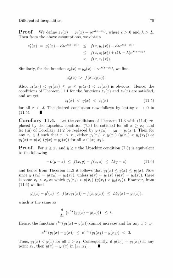
Differential Inequalities 79
Proof. We define z1(x) = y1(x) − εeλ(x−x0), where ε > 0 and λ > L.Then from the above assumptions, we obtain
z′1(x) = y′
1(x) − ελeλ(x−x0) ≤ f(x, y1(x)) − ελeλ(x−x0)
≤ f(x, z1(x)) + ε(L− λ)eλ(x−x0)
< f(x, z1(x)).
Similarly, for the function z2(x) = y2(x) + εeλ(x−x0), we find
z′2(x) > f(x, z2(x)).
Also, z1(x0) < y1(x0) ≤ y0 ≤ y2(x0) < z2(x0) is obvious. Hence, theconditions of Theorem 11.1 for the functions z1(x) and z2(x) are satisfied,and we get
z1(x) < y(x) < z2(x) (11.5)
for all x ∈ J. The desired conclusion now follows by letting ε → 0 in(11.5).
Corollary 11.4. Let the conditions of Theorem 11.3 with (11.4) re-placed by the Lipschitz condition (7.3) be satisfied for all x ≥ x0, andlet (iii) of Corollary 11.2 be replaced by y1(x0) = y0 = y2(x0). Then forany x1 ∈ J such that x1 > x0, either y1(x1) < y(x1) (y(x1) < y2(x1)) ory1(x) = y(x) (y(x) = y2(x)) for all x ∈ [x0, x1].
Proof. For x ≥ x0 and y ≥ z the Lipschitz condition (7.3) is equivalentto the following
−L(y − z) ≤ f(x, y) − f(x, z) ≤ L(y − z) (11.6)
and hence from Theorem 11.3 it follows that y1(x) ≤ y(x) ≤ y2(x). Nowsince y1(x0) = y(x0) = y2(x0), unless y(x) = y1(x) (y(x) = y2(x)), thereis some x1 > x0 at which y1(x1) < y(x1) (y(x1) < y2(x1)). However, from(11.6) we find
y′1(x) − y′(x) ≤ f(x, y1(x)) − f(x, y(x)) ≤ L(y(x) − y1(x)),
which is the same as
d
dx
(eLx(y1(x) − y(x))
) ≤ 0.
Hence, the function eLx(y1(x) − y(x)) cannot increase and for any x > x1
eLx(y1(x) − y(x)) ≤ eLx1(y1(x1) − y(x1)) < 0.
Thus, y1(x) < y(x) for all x > x1. Consequently, if y(x1) = y1(x1) at anypoint x1, then y(x) = y1(x) in [x0, x1].

80 Lecture 11
For our next application of Theorem 11.1, we need the following defini-tion.
Definition 11.1. A solution r(x) (ρ(x)) of the initial value problem(7.1) which exists in an interval J is said to be a maximal (minimal) solutionif for an arbitrary solution y(x) of (7.1) existing in J, the inequality y(x) ≤r(x) (ρ(x) ≤ y(x)) holds for all x ∈ J.
Obviously, if the maximal and minimal solutions exist, then these areunique. The existence of these solutions is proved in the following theorem.
Theorem 11.5. Let f(x, y) be continuous in S+ : x0 ≤ x ≤ x0 +a, |y − y0| ≤ b and hence there exists a M > 0 such that |f(x, y)| ≤ M forall (x, y) ∈ S+. Then there exist a maximal solution r(x) and a minimalsolution ρ(x) of (7.1) in the interval [x0, x0 +α], where α = mina, b/(2M+b).Proof. We shall prove the existence of the maximal solution r(x) only.Let 0 < ε ≤ b/2, and consider the initial value problem
y′ = f(x, y) + ε, y(x0) = y0 + ε. (11.7)
Since the function fε(x, y) = f(x, y)+ ε is continuous in Sε : x0 ≤ x ≤ x0 +a, |y− (y0 +ε)| ≤ b/2, and Sε ⊆ S+ we find that |fε(x, y)| ≤ M+b/2 in Sε.Hence, from Corollary 9.2 it follows that the problem (11.7) has a solutiony(x, ε) in the interval [x0, x0 + α], where α = mina, b/(2M + b). For0 < ε2 < ε1 ≤ ε, we have y(x0, ε2) < y(x0, ε1) and y′(x, ε2) = f(x, y(x, ε2))+ε2, y
′(x, ε1) > f(x, y(x, ε1)) + ε2, x ∈ [x0, x0 + α]. Thus, Theorem 11.1 isapplicable and we have y(x, ε2) < y(x, ε1) for all x ∈ [x0, x0 + α]. Nowas in Theorem 9.1 it is easy to see that the family of functions y(x, ε)is equicontinuous and uniformly bounded in [x0, x0 + α], therefore, fromTheorem 7.10 there exists a decreasing sequence εn such that εn → 0 asn → ∞, and limn→∞ y(x, εn) exists uniformly in [x0, x0+α]. We denote thislimiting function by r(x). Obviously, r(x0) = y0, and the uniform continuityof f, with
y(x, εn) = y0 + εn +∫ x
x0
[f(t, y(t, εn)) + εn]dt
yields r(x) as a solution of (7.1).
Finally, we shall show that r(x) is the maximal solution of (7.1) in[x0, x0 + α]. For this, let y(x) be any solution of (7.1) in [x0, x0 + α]. Theny(x0) = y0 < y0 + ε = y(x0, ε), and y′(x) < f(x, y(x)) + ε, y′(x, ε) =f(x, y(x, ε)) + ε for all x ∈ [x0, x0 + α] and 0 < ε ≤ b/2. Thus, fromTheorem 11.1 it follows that y(x) < y(x, ε), x ∈ [x0, x0 + α]. Now theuniqueness of the maximal solution shows that y(x, ε) tends uniformly tor(x) in [x0, x0 + α] as ε → 0.

Differential Inequalities 81
Obviously, the process of continuation of the solutions of (7.1) discussedin Lecture 9 can be employed for the maximal solution r(x) as well as forthe minimal solution ρ(x).
Example 11.2. For the initial value problem y′ = |y|1/2, y(0) = 0 itis clear that r(x) = x2/4, ρ(x) = 0 if x ≥ 0; r(x) = 0, ρ(x) = −x2/4 ifx ≤ 0; and
r(x) =
⎧⎨⎩
x2
4if x ≥ 0
0 if x ≤ 0,ρ(x) =
⎧⎨⎩
0 if x ≥ 0
−x2
4if x ≤ 0.
Finally, as an application of maximal solution r(x) we shall prove thefollowing theorem.
Theorem 11.6. Let f(x, y) be continuous in the domain D, and letr(x) be the maximal solution of (7.1) in the interval J = [x0, x0 + a). Also,let y(x) be a solution of the differential inequality
y′(x) ≤ f(x, y(x)) (11.8)
in J. Then y(x0) ≤ y0 implies that
y(x) ≤ r(x) for all x ∈ J. (11.9)
Proof. For x1 ∈ (x0, x0+a) an argument similar to that for Theorem 11.5shows that there exists a maximal solution r(x, ε) of (11.7) in [x0, x1] for allsufficiently small ε > 0 and limε→0 r(x, ε) = r(x) uniformly in x ∈ [x0, x1].Now for (11.7) and (11.8) together with y(x0) ≤ y0 < r(x0, ε), Theorem11.1 gives
y(x) < r(x, ε) (11.10)
in [x0, x1]. The inequality (11.9) follows by taking ε → 0 in (11.10).
Problems
11.1. Give an example to show that in Theorem 11.1 strict inequalitiescannot be replaced with equalities.
11.2. Let y(x) be a solution of the initial value problem y′ = y −y2, y(0) = y0, 0 < y0 < 1. Show that y0 < y(x) ≤ 1 for all x ∈ (0,∞).
11.3. Let y(x) be a solution of the initial value problem y′ = y2 −x, y(0) = 1. Show that 1 + x < y(x) < 1/(1 − x) for all x ∈ (0, 1).
11.4. Let f1(x, y) and f2(x, y) be continuous in the domain D, andf1(x, y) < f2(x, y) for all (x, y) ∈ D. Further, let y1(x) and y2(x) be the

82 Lecture 11
solutions of the DEs y′1 = f1(x, y1) and y′
2 = f2(x, y2), respectively, existingin J = [x0, x0 + a) such that y1(x0) < y2(x0). Show that y1(x) < y2(x) forall x ∈ J.
∗11.5. For a given function y(x) the Dini derivatives are defined asfollows:
D+y(x) = lim suph→0+
(y(x+ h) − y(x)
h
)(upper-right derivative)
D+y(x) = lim infh→0+
(y(x+ h) − y(x)
h
)(lower-right derivative)
D−y(x) = lim suph→0−
(y(x+ h) − y(x)
h
)(upper-left derivative)
D−y(x) = lim infh→0−
(y(x+ h) − y(x)
h
)(lower-left derivative).
In case D+y(x) = D+y(x), the right-hand derivative denoted by y′+(x)
exists and y′+(x) = D+y(x) = D+y(x).
In case D−y(x) = D−y(x), the left-hand derivative denoted by y′−(x)
exists and y′−(x) = D−y(x) = D−y(x).
In case y′+(x) = y′
−(x), the derivative exists and y′(x) = y′+(x) = y′
−(x).Conversely, if y′(x) exists, then all the four Dini derivatives are equal.
Clearly, D+y(x) ≤ D+y(x) and D−y(x) ≤ D−y(x). Show the following:
(i) If y(x) ∈ C[x0, x0 + a), then a necessary and sufficient condition fory(x) to be nonincreasing in [x0, x0 + a) is that Dy(x) ≤ 0, where D is afixed Dini derivative.(ii) If y(x), z(x) ∈ C[x0, x0 + a), and Dy(x) ≤ z(x), where D is a fixedDini derivative, then D−y(x) ≤ z(x).(iii) Theorem 11.1 remains true when in the inequalities (11.1) the deriva-tive is replaced by any fixed Dini derivative.(iv) If y(x) ∈ C(1)[x0, x0+a), then z(x) = |y(x)| has a right-hand derivativez′+(x) and z′
+(x) ≤ |y′(x)|.∗11.6. Let f(x, y) be continuous in the domain D, and y(x) be a
solution of the differential inequality D−y ≤ f(x, y) in (x0 − a, x0] andy(x0) ≥ y0. Show that ρ(x) ≤ y(x) as far as the minimal solution ρ(x) of(7.1) exists to the left of x0.
Answers or Hints
11.1. The problem y′ = y2/3, y(0) = 0 has solutions y1(x) = x3/27, y2(x)

Differential Inequalities 83
≡ 0 in [0,∞). For these functions equalities hold everywhere in Theorem11.1. However, x3/27 ≤ 0 in (0,∞).
11.2. Let y1(x) = y0, y2(x) = 1 + ε, ε > 0 and use Theorem 11.1 andCorollary 11.2.
11.3. Let y1(x) = 1 + x, y2(x) = 1/(1 − x) and use Corollary 11.2.
11.4. Define f(x, y) = (f1(x, y) + f2(x, y))/2 so that y′1 < f(x, y1), y′
2 >f(x, y2) and y1(x0) < y2(x0). Now use Theorem 11.1.

Lecture 12Continuous Dependence
on Initial Conditions
The initial value problem (7.1) describes a model of a physical problemin which often some parameters such as lengths, masses, temperatures, etc.,are involved. The values of these parameters can be measured only up tocertain degree of accuracy. Thus, in (7.1) the initial condition (x0, y0) aswell as the function f(x, y) may be subject to some errors either by necessityor for convenience. Hence, it is important to know how the solution of (7.1)changes when (x0, y0) and f(x, y) are slightly altered. We shall answer thisquestion quantitatively in the following theorem.
Theorem 12.1. Let the following conditions be satisfied:
(i) f(x, y) is continuous and bounded by M in a domain D containingthe points (x0, y0) and (x1, y1).
(ii) f(x, y) satisfies a uniform Lipschitz condition (7.3) in D.
(iii) g(x, y) is continuous and bounded by M1 in D.
(iv) y(x) and z(x), the solutions of the initial value problems (7.1) and
z′ = f(x, z) + g(x, z), z(x1) = y1,
respectively, exist in an interval J containing x0 and x1.
Then for all x ∈ J , the following inequality holds:
|y(x) − z(x)| ≤(
|y0 − y1| + (M +M1)|x1 − x0| +1LM1
)
× exp (L|x− x0|) − 1LM1.
(12.1)
Proof. From Theorem 7.1 for all x ∈ J it follows that
z(x) = y1 +∫ x
x1
[f(t, z(t)) + g(t, z(t))]dt
= y1 +∫ x
x0
f(t, z(t))dt+∫ x0
x1
f(t, z(t))dt+∫ x
x1
g(t, z(t))dt
R.P. Agarwal and D. O’Regan, An Introduction to Ordinary Differential Equations,
84doi: 10.1007/978-0-387-71276-5_12, © Springer Science + Business Media, LLC 2008

Continuous Dependence on Initial Conditions 85
and hence, we find
y(x) − z(x) = y0 − y1 +∫ x
x0
[f(t, y(t)) − f(t, z(t))]dt
+∫ x1
x0
f(t, z(t))dt−∫ x
x1
g(t, z(t))dt.(12.2)
Now taking absolute values on both sides of (12.2) and using the hypotheses,we get
|y(x) − z(x)| ≤ |y0 − y1| + (M +M1)|x1 − x0| +M1|x− x0|+L
∣∣∣∣∫ x
x0
|y(t) − z(t)|dt∣∣∣∣ . (12.3)
Inequality (12.3) is exactly the same as that considered in Corollary7.6 with c0 = |y0 − y1| + (M + M1)|x1 − x0|, c1 = M1, c2 = L andu(x) = |y(x) − z(x)|, and hence the inequality (12.1) follows.
From the inequality (12.1) it is apparent that the difference betweenthe solutions y(x) and z(x) in the interval J is small provided the changesin the initial point (x0, y0) as well as in the function f(x, y) do not exceedprescribed amounts. Thus, the statement “if the function f(x, y) and theinitial point (x0, y0) vary continuously, then the solutions of (7.1) varycontinuously” holds. It is also clear that the solution z(x) of the initialvalue problem z′ = f(x, z) + g(x, z), z(x1) = y1 need not be unique in J.
Example 12.1. Consider the initial value problem
y′ = sin(xy), y(0) = 1 (12.4)
in the rectangle S : |x| ≤ 1/2, |y − 1| ≤ 1/2. To apply Theorem 8.1 wenote that a = 1/2, b = 1/2 and maxS | sin(xy)| ≤ 1 ≤ M, and fromTheorem 7.2 the function sin(xy) satisfies the Lipschitz condition (7.3) inS, and maxS |x cos(xy)| = 1/2 = L. Thus, the problem (12.4) has a uniquesolution in the interval |x| ≤ h ≤ 1/2.
As an approximation of the initial value problem (12.4), we consider
z′ = xz, z(0) = 1.1, (12.5)
which also has a unique solution z(x) = 1.1 exp(x2/2) in the interval |x| ≤1/2. Now by Taylor’s formula, we find
|g(x, y)| = | sin(xy) − xy| ≤ 16|xy|3 ≤ 1
6
(12
)3(32
)3
=9
128= M1.

86 Lecture 12
Using Theorem 12.1 for the above initial value problems, we obtain anupper error bound for the difference between the solutions y(x) and z(x)
|y(x) − z(x)| ≤(
0.1 +964
)exp
( |x|2
)− 9
64for all |x| ≤ 1
2.
To emphasize the dependence of the initial point (x0, y0), we shall denotethe solution of the initial value problem (7.1) as y(x, x0, y0). In our nextresult we shall show that y(x, x0, y0) is differentiable with respect to y0.
Theorem 12.2. Let the following conditions be satisfied:
(i) f(x, y) is continuous and bounded by M in a domain D containingthe point (x0, y0).(ii) ∂f(x, y)/∂y exists, continuous and bounded by L in D.(iii) The solution y(x, x0, y0) of the initial value problem (7.1) exists in aninterval J containing x0.
Then we have that y(x, x0, y0) is differentiable with respect to y0 and z(x) =∂y(x, x0, y0)/∂y0 is the solution of the initial value problem
z′ =∂f
∂y(x, y(x, x0, y0))z (12.6)
z(x0) = 1. (12.7)
The DE (12.6) is called the variational equation corresponding to the solu-tion y(x, x0, y0).
Proof. Let (x0, y1) ∈ D be such that the solution y(x, x0, y1) of theinitial value problem y′ = f(x, y), y(x0) = y1 exists in an interval J1. Thenfor all x ∈ J2 = J ∩ J1, Theorem 12.1 implies that
|y(x, x0, y0) − y(x, x0, y1)| ≤ |y0 − y1|eL|x−x0|,
i.e., |y(x, x0, y0) − y(x, x0, y1)| → 0 as |y0 − y1| → 0.
Now for all x ∈ J2 it is easy to verify that
y(x, x0, y0) − y(x, x0, y1) − z(x)(y0 − y1)
=∫ x
x0
[f(t, y(t, x0, y0))−f(t, y(t, x0, y1))− ∂f
∂y(t, y(t, x0, y0))z(t)(y0−y1)
]dt
=∫ x
x0
∂f
∂y(t, y(t, x0, y0))[y(t, x0, y0) − y(t, x0, y1) − z(t)(y0 − y1)]dt
+∫ x
x0
δy(t, x0, y0), y(t, x0, y1)dt,

Continuous Dependence on Initial Conditions 87
where δy(x, x0, y0), y(x, x0, y1) → 0 as |y(x, x0, y0) − y(x, x0, y1)| → 0,i.e., as |y0 − y1| → 0.
Hence, we find that
|y(x, x0, y0) − y(x, x0, y1) − z(x)(y0 − y1)|≤ L
∣∣∣∣∫ x
x0
|y(t, x0, y0) − y(t, x0, y1) − z(t)(y0 − y1)|dt∣∣∣∣+ o(|y0 − y1|).
Now applying Corollary 7.6, we get
|y(x, x0, y0) − y(x, x0, y1) − z(x)(y0 − y1)| ≤ o(|y0 − y1|) exp(L|x− x0|).
Thus, |y(x, x0, y0) − y(x, x0, y1) − z(x)(y0 − y1)| → 0 as |y0 − y1| → 0.This completes the proof.
In our next result we shall show that the conditions of Theorem 12.2 arealso sufficient for the solution y(x, x0, y0) to be differentiable with respectto x0.
Theorem 12.3. Let the conditions of Theorem 12.2 be satisfied. Thenthe solution y(x, x0, y0) is differentiable with respect to x0 and z(x) =∂y(x, x0, y0)/∂x0 is the solution of the variational equation (12.6), satisfyingthe initial condition
z(x0) = − f(x0, y0). (12.8)
Proof. The proof is similar to that of Theorem 12.2.
We note that the variational equation (12.6) can be obtained directlyby differentiating the relation y′(x, x0, y0) = f(x, y(x, x0, y0)) with respectto y0 (or x0). Further, since y(x0, x0, y0) = y0, differentiation with respectto y0 gives the initial condition (12.7). To obtain (12.8), we begin with theintegral equation
y(x, x0, y0) = y0 +∫ x
x0
f(t, y(t, x0, y0))dt
and differentiate it with respect to x0, to obtain
∂y(x, x0, y0)∂x0
∣∣∣∣x=x0
= − f(x0, y0).
Finally, in this lecture we shall consider the initial value problem
y′ = f(x, y, λ), y(x0) = y0, (12.9)
where λ ∈ IR is a parameter. The proof of the following theorem is verysimilar to earlier results.

88 Lecture 12
Theorem 12.4. Let the following conditions be satisfied:
(i) f(x, y, λ) is continuous and bounded by M in a domain D ⊂ IR3
containing the point (x0, y0, λ0).(ii) ∂f(x, y, λ)/∂y, ∂f(x, y, λ)/∂λ exist, continuous and bounded, respec-tively, by L and L1 in D.
Then the following hold:
(1) There exist positive numbers h and ε such that given any λ in theinterval |λ − λ0| ≤ ε, there exits a unique solution y(x, λ) of the initialvalue problem (12.9) in the interval |x− x0| ≤ h.(2) For all λ1, λ2 in the interval |λ − λ0| ≤ ε, and x in |x − x0| ≤ h thefollowing inequality holds:
|y(x, λ1) − y(x, λ2)| ≤ L1|λ1 − λ2|L
(exp(L|x− x0|) − 1) . (12.10)
(3) The solution y(x, λ) is differentiable with respect to λ and z(x, λ) =∂y(x, λ)/∂λ is the solution of the initial value problem
z′(x, λ) =∂f
∂y(x, y(x, λ), λ)z(x, λ) +
∂f
∂λ(x, y(x, λ), λ), (12.11)
z(x0, λ) = 0. (12.12)
If λ is such that |λ− λ0| is sufficiently small, then we have a first-orderapproximation of the solution y(x, λ) given by
y(x, λ) y(x, λ0) + (λ− λ0)[∂y
∂λ(x, λ)
]λ=λ0
= y(x, λ0) + (λ− λ0)z(x, λ0).(12.13)
We illustrate this important idea in the following example.
Example 12.2. Consider the initial value problem
y′ = λy2 + 1, y(0) = 0 (λ ≥ 0) (12.14)
for which the solution y(x, λ) = (1/√λ) tan(
√λx) exists in the inter-
val (−π/(2√λ), π/(2
√λ)). Let in (12.14) the parameter λ = 0, so that
y(x, 0) = x. Since ∂f/∂y = 2λy and ∂f/∂λ = y2, the initial value problemcorresponding to (12.11), (12.12) is
z′(x, 0) = x2, z(0, 0) = 0,

Continuous Dependence on Initial Conditions 89
whose solution is z(x, 0) = x3/3. Thus, for λ near zero, (12.13) gives theapproximation
y(x, λ) =1√λ
tan(√λ x) x+ λ
x3
3.
Problems
12.1. Let y(x, λ) denote the solution of the initial value problem
y′ + p(x)y = q(x), y(x0) = λ
in the interval x0 ≤ x < ∞. Show that for each fixed x > x0 and for eachpositive number ε there exists a positive number δ such that |y(x, λ+∆λ)−y(x, λ)| ≤ ε, whenever |∆λ| ≤ δ, i.e., the solution y(x, λ) is continuous withrespect to the parameter λ.
12.2. Prove Theorem 12.3.
12.3. Prove Theorem 12.4.
12.4. For the initial value problem
y′ = x+ ex sin(xy), y(0) = 0 = y0
estimate the variation of the solution in the interval [0, 1] if y0 is perturbedby 0.01.
12.5. For the initial value problem y′ = λ+ cos y, y(0) = 0 obtain anupper estimate for |y(x, λ1) − y(x, λ2)| in the interval [0, 1].
12.6. For sufficiently small λ find a first-order approximation of thesolution y(x, λ) of the initial value problem y′ = y + λ(x+ y2), y(0) = 1.
12.7. State and prove an analog of Theorem 12.1 for the initial valueproblem (7.9).
12.8. Find the error in using the approximate solution
y(x) = exp(−x3/6)
for the initial value problem y′′ +xy = 0, y(0) = 1, y′(0) = 0 in the interval|x| ≤ 1/2.
Answers or Hints
12.1. Let z(x) = y(x, λ+∆λ)−y(x, λ). Then z′(x)+p(x)z(x) = 0, z(x0) =∆λ, whose solution is z(x) = ∆λ exp
(− ∫ x
x0p(t)dt
).

90 Lecture 12
12.2. The proof is similar to that of Theorem 12.2.
12.3. For the existence and uniqueness of solutions of (12.9) see the remarkfollowing Theorem 16.7. To prove inequality (12.10) use Corollary 7.6.
12.4. 0.01ee.
12.5. |λ1 − λ2|(e− 1).
12.6. ex + λ(e2x − x− 1).
12.7. The result corresponding to Theorem 12.1 for (7.9) can be statedas follows: Let the conditions (i)–(iii) of Theorem 12.1 be satisfied and(iv)′ y(x) and z(x), the solutions of (7.9) and z′′ = f(x, z)+g(x, z), z(x1) =z0, z
′(x1) = z1, respectively, exist in J = (α, β) containing x0 and x1. Thenfor all x ∈ J , the following inequality holds:
|y(x) − z(x)| ≤ [|y0 − z0| + |x1 − x0|(|z1| + (β − α)(M +M1))] + γ× exp(L(β − α)|x− x0|) − γ,
where γ = [|y1 − z1| +M1(β − α)]/L(β − α).
12.8. (1/512)e1/12.

Lecture 13Preliminary Results from
Algebra and Analysis
For future reference we collect here several fundamental concepts andresults from algebra and analysis.
A function Pn(x) defined by
Pn(x) = a0 + a1x+ · · · + anxn =
n∑i=0
aixi, an = 0
where ai ∈ IR, 0 ≤ i ≤ n, is called a polynomial of degree n in x. IfPn(x1) = 0, then the number x = x1 is called a zero of Pn(x). The followingfundamental theorem of algebra of complex numbers is valid.
Theorem 13.1. Every polynomial of degree n ≥ 1 has at least onezero.
Thus, Pn(x) has exactly n zeros; however, some of these may be thesame, i.e., Pn(x) can be written as
Pn(x) = an(x− x1)r1(x− x2)r2 · · · (x− xk)rk , ri ≥ 1, 1 ≤ i ≤ k,
where∑k
i=1 ri = n. If ri = 1, then xi is called a simple zero, and if ri >1, then multiple zero of multiplicity ri. Thus, if xi is a multiple zero ofmultiplicity ri, then P (j)(xi) = 0, 0 ≤ j ≤ ri − 1 and P (ri)(xi) = 0.
A rectangular table ofm×n elements arranged in m rows and n columns⎡⎢⎢⎣
a11 a12 · · · a1n
a21 a22 · · · a2n
· · ·am1 am2 · · · amn
⎤⎥⎥⎦
is called an m × n matrix and in short represented as A = (aij). We shallmainly deal with square matrices (m = n), row matrices or row vectors(m = 1), and column matrices or column vectors (n = 1).
A matrix with aij = 0, 1 ≤ i, j ≤ n, is called null or zero matrix, whichwe shall denote by 0.
R.P. Agarwal and D. O’Regan, An Introduction to Ordinary Differential Equations,
91doi: 10.1007/978-0-387-71276-5_13, © Springer Science + Business Media, LLC 2008

92 Lecture 13
A matrix with aij = 0, 1 ≤ i = j ≤ n is called a diagonal matrix ; if, inaddition, aii = 1, 1 ≤ i ≤ n, then it is an identity matrix which we shalldenote by I.
The transpose of a matrix denoted by AT is a matrix with elements aji.A matrix is called symmetric if A = AT .
The sum of two matrices A = (aij) and B = (bij) is a matrix C = (cij)with elements cij = aij + bij .
Let α be a constant and A be a matrix; then αA is a matrix C = (cij)with elements cij = αaij .
Let A and B be two matrices; then the product AB is a matrix C = (cij)with elements cij =
∑nk=1 aikbkj . Note that in general AB = BA, but
(AB)T = BTAT .
The trace of a matrix A is denoted by TrA and it is the sum of thediagonal elements, i.e.,
TrA =n∑
i=1
aii.
Associated with an n × n matrix A = (aij) there is a scalar called thedeterminant of A
detA =
∣∣∣∣∣∣∣∣a11 a12 · · · a1n
a21 a22 · · · a2n
· · ·an1 an2 · · · ann
∣∣∣∣∣∣∣∣.
An (n − 1) × (n − 1) determinant obtained by deleting ith row and jthcolumn of the matrix A is called the minor aij of the element aij . Wedefine the cofactor of aij as αij = (−1)i+j aij . In terms of cofactors thedeterminant of A is defined as
detA =n∑
j=1
aijαij =n∑
i=1
aijαij . (13.1)
Further,n∑
j=1
aijαkj = 0 if i = k. (13.2)
The following properties of determinants are fundamental:
(i) If two rows (or columns) of A are equal or have a constant ratio, thendetA = 0.(ii) If any two consecutive rows (or columns) of A are interchanged, thenthe determinant of the new matrix A1 is −detA.(iii) If a row (or column) of A is multiplied by a constant α, then thedeterminant of the new matrix A1 is α det A.

Preliminary Results from Algebra and Analysis 93
(iv) If a constant multiple of one row (or column) of A is added to another,then the determinant of the new matrix A1 is unchanged.(v) detAT = detA.(vi) detAB = (detA)(detB).
A linear system of n equations in n unknowns is a set of equations ofthe following form:
a11u1 + · · · + a1nun = b1a21u1 + · · · + a2nun = b2· · ·an1u1 + · · · + annun = bn,
(13.3)
where aij and bi, 1 ≤ i, j ≤ n, are given real numbers and n unknowns areui, 1 ≤ i ≤ n.
The system (13.3) can be written in a compact form as
Au = b, (13.4)
where A is an n×n matrix (aij), b is an n×1 vector (bi), and u is an n×1unknown vector (ui). If b = 0, the system (13.4) is called homogeneous,otherwise it is called nonhomogeneous.
The following result provides a necessary and sufficient condition for thesystem (13.4) to have a unique solution.
Theorem 13.2. The system (13.4) has a unique solution if and onlyif detA = 0. Alternatively, if the homogeneous system has only the trivialsolution (u = 0), then detA = 0.
If detA = 0 then the matrix A is said to be singular ; otherwise, non-singular. Thus, the homogeneous system has nontrivial solutions if andonly if the matrix A is singular. The importance of this concept lies inthe fact that a nonsingular matrix A possesses a unique inverse denotedby A−1. This matrix has the property that AA−1 = A−1A = I. Moreover,A−1 = (AdjA)/(detA), where AdjA is an n×n matrix with elements αji.
A real vector space (linear space) V is a collection of objects calledvectors, together with an addition and a multiplication by real numberswhich satisfy the following axioms:
1. Given any pair of vectors u and v in V there exists a unique vector u+vin V called the sum of u and v. It is required that
(i) addition be commutative, i.e., u+ v = v + u;(ii) addition be associative, i.e., u+ (v + w) = (u+ v) + w;(iii) there exists a vector 0 in V (called the zero vector) such that u+ 0 =0 + u = u for all u in V ;

94 Lecture 13
(iv) for each u in V , there exists a vector −u in V such that u+(−u) = 0.
2. Given any vector u in V and any real number α, there exists a uniquevector α u in V called the product or scalar product of α and u. Given anytwo real numbers α and β it is required that
(i) α(u+ v) = αu+ αv,
(ii) (α+ β)u = αu+ βu,
(iii) (αβ)u = α(βu),(iv) 1u = u.
A complex vector space is defined analogously.
There are numerous examples of real (complex) vector spaces which areof interest in analysis, some of these are the following:
(a) The space IRn(Cn) is a real (complex) vector space if for all u =(u1, . . . , un), v = (v1, . . . , vn) in IRn(Cn), and α ∈ IR(C),
u+ v = (u1 + v1, . . . , un + vn)αu = (αu1, . . . , α un).
(b) The space of all continuous functions in an interval J denoted by C(J)is a real vector space if for all y(x), z(x) ∈ C(J), and α ∈ IR,
(y + z)(x) = y(x) + z(x)(αy)(x) = αy(x).
(c) The function u(x) = (u1(x), . . . , un(x)), or (u1(x), . . . , un(x))T , whereui(x), 1 ≤ i ≤ n, are continuous in an interval J , is called a vector-valuedfunction. The space of all continuous vector-valued functions in J denotedby Cn(J) is a real vector space if for all u(x), v(x) ∈ Cn(J) and α ∈ IR
(u+ v)(x) = (u1(x) + v1(x), . . . , un(x) + vn(x))(αu)(x) = (αu1(x), . . . , αun(x)).
(d) The matrix A(x) = (aij(x)), where aij(x), 1 ≤ i, j ≤ n, are continuousin an interval J , is called a matrix-valued function. The space of all con-tinuous matrix-valued functions in J denoted by Cn×n(J) is a real vectorspace if for all A(x), B(x) ∈ Cn×n(J) and α ∈ IR
(A+B)(x) = (aij(x) + bij(x))(αA)(x) = (αaij(x)).
The space of all m (nonnegative integer) times continuously differen-tiable functions in J denoted by C(m)(J) is also a vector space. Similarly,C
(m)n (J) and C
(m)n×n(J), where the derivatives of the function u(x) and of

Preliminary Results from Algebra and Analysis 95
the matrix A(x) are defined as u′(x) = (u′i(x)) and A′(x) = (a′
ij(x)), re-spectively, are vector spaces.
From the definition of determinants it is clear that for a given matrixA(x) ∈ C
(m)n×n(J) the function detA(x) ∈ C(m)(J). Later we shall need
the differentiation of the function det A(x) which we shall now compute byusing the expansion of detA given in (13.1). Since
detA(x) =n∑
j=1
aij(x)αij(x),
it follows that∂ detA(x)∂aij(x)
= αij(x),
and hence
(detA(x))′ =n∑
j=1
n∑i=1
∂ detA(x)∂aij(x)
daij(x)dx
=n∑
j=1
n∑i=1
αij(x)a′ij(x),
which is equivalent to
(detA(x))′ =
∣∣∣∣∣∣∣∣a′11(x) · · · a′
1n(x)a21(x) · · · a2n(x)
· · ·an1(x) · · · ann(x)
∣∣∣∣∣∣∣∣+
∣∣∣∣∣∣∣∣a11(x) · · · a1n(x)a′21(x) · · · a′
2n(x)· · ·
an1(x) · · · ann(x)
∣∣∣∣∣∣∣∣+ · · ·
+
∣∣∣∣∣∣∣∣a11(x) · · · a1n(x)a21(x) · · · a2n(x)
· · ·a′
n1(x) · · · a′nn(x)
∣∣∣∣∣∣∣∣.
(13.5)Let V be a vector space and let v1, . . . , vm ∈ V be fixed vectors.
These vectors are said to be linearly independent if the choice of con-stants α1, . . . , αm for which α1v
1 + · · · + αmvm = 0 is the trivial choice,
i.e., α1 = · · · = αm = 0. Conversely, these vectors are said to be lin-early dependent if there exist constants α1, . . . , αm not all zero such thatα1v
1 + · · · + αmvm = 0. The set v1, . . . , vm is a basis for V if for ev-
ery v ∈ V , there is a unique choice of constants α1, . . . , αm for whichv = α1v
1 + · · ·+αmvm. Note that this implies v1, . . . , vm is independent. If
such a finite basis exists, we say that V is finite dimensional. Otherwise, it iscalled infinite dimensional. If V is a vector space with a basis v1, . . . , vm,then every basis for V will contain exactly m vectors. The number m iscalled the dimension of V. A nonempty subset W ⊂ V is called a subspaceif W is closed under the operations of addition and multiplication in V.
For a given n×nmatrix A, its columns (rows) generate a subspace whosedimension is called the column (row) rank of A. It is well known that the

96 Lecture 13
row rank and the column rank of A are equal to the same number r. Thisnumber r is called the rank of A. If r = n, i.e., detA = 0, then Theorem 13.2implies that the system (13.4) has a unique solution. However, if r < n,then (13.4) may not have any solution. In this case, the following resultprovides necessary and sufficient conditions for the system (13.4) to haveat least one solution.
Theorem 13.3. If the rank of A is n − m (1 ≤ m ≤ n), then thesystem (13.4) possesses a solution if and only if
Bb = 0, (13.6)
where B is an m × n matrix whose row vectors are linearly independentvectors bi, 1 ≤ i ≤ m, satisfying biA = 0.
Further, in the case when (13.6) holds, any solution of (13.4) can beexpressed as
u =m∑
i=1
ciui + Sb,
where ci, 1 ≤ i ≤ m, are arbitrary constants, ui, 1 ≤ i ≤ m, are m linearlyindependent column vectors satisfying Aui = 0, and S is an n × n matrixindependent of b such that ASv = v for any column vector v satisfyingBv = 0.
The matrix S in the above result is not unique.

Lecture 14Preliminary Results from
Algebra and Analysis (Contd.)
The number λ, real or complex, is called an eigenvalue of the matrixA if there exists a nonzero real or complex vector v such that Av = λv.The vector v is called an eigenvector corresponding to the eigenvalue λ.From Theorem 13.2, λ is an eigenvalue of A if and only if it is a solutionof the characteristic equation p(λ) = det (A − λI) = 0. Since the matrixA is n × n, p(λ) is a polynomial of degree exactly n, and it is called thecharacteristic polynomial of A. Hence, from Theorem 13.1 it follows that Ahas exactly n eigenvalues counting their multiplicities.
In the case when the eigenvalues λ1, . . . , λn of A are distinct it is easy tofind the corresponding eigenvectors v1, . . . , vn. For this, first we note thatfor the fixed eigenvalue λj of A at least one of the cofactors of (aii − λj)in the matrix (A − λjI) is nonzero. If not, then from (13.5) it followsthat p′(λ) = −[cofactor of (a11 − λ)] − · · · − [cofactor of (ann − λ)], andhence p′(λj) = 0; i.e., λj was a multiple root, which is a contradiction toour assumption that λj is simple. Now let the cofactor of (akk − λj) bedifferent from zero, then one of the possible nonzero solution of the system(A − λjI)vj = 0 is vj
i = cofactor of aki in (A − λjI), 1 ≤ i ≤ n, i = k,
vjk = cofactor of (akk − λj) in (A − λjI). Since for this choice of vj , it
follows from (13.2) that every equation, except the kth one, of the system(A− λjI)vj = 0 is satisfied, and for the kth equation from (13.1), we have
n∑i = 1i = k
aki[cofactor of aki]+(akk−λj)[cofactor of (akk−λj)] = det (A−λjI),
which is also zero. In conclusion this vj is the eigenvector corresponding tothe eigenvalue λj .
Example 14.1. The characteristic polynomial for the matrix
A =
⎡⎣ 2 1 0
1 3 10 1 2
⎤⎦
is p(λ) = −λ3 + 7λ2 − 14λ + 8 = −(λ − 1)(λ − 2)(λ − 4) = 0. Thus, theeigenvalues are λ1 = 1, λ2 = 2 and λ3 = 4. To find the corresponding
R.P. Agarwal and D. O’Regan, An Introduction to Ordinary Differential Equations,
97doi: 10.1007/978-0-387-71276-5_14 , © Springer Science + Business Media, LLC 2008

98 Lecture 14
eigenvectors we have to consider the systems (A − λiI)vi = 0, i = 1, 2, 3.For λ1 = 1, we find
(A− λ1I) =
⎡⎣ 1 1 0
1 2 10 1 1
⎤⎦ .
Since the cofactor of (a11 − λ1) = 1 = 0, we can take v11 = 1, and then
v12 = cofactor of a12 = −1, v1
3 = cofactor of a13 = 1, i.e., v1 = [1 − 1 1]T .
Next for λ2 = 2 we have
(A− λ2I) =
⎡⎣ 0 1 0
1 1 10 1 0
⎤⎦ .
Since the cofactor of (a22 −λ2) = 0, the choice v22 = cofactor of (a22 −λ2) is
not correct. However, cofactor of (a11−λ2) = cofactor of (a33−λ2) = −1 =0 and we can take v2
1 = −1 (v23 = −1), then v2
2 = cofactor of a12 = 0, v23 =
cofactor of a13 = 1 (v21 = cofactor of a31 = 1, v2
2 = cofactor of a32 = 0),i.e., v2 = [−1 0 1]T ([1 0 − 1]T ).
Similarly, we can find v3 = [1 2 1]T .
For the eigenvalues and eigenvectors of an n× n matrix A, we have thefollowing basic result.
Theorem 14.1. Let λ1, . . . , λm be distinct eigenvalues of an n × nmatrix A and v1, . . . , vm be corresponding eigenvectors. Then v1, . . . , vm
are linearly independent.
Since p(λ) is a polynomial of degree n, and Am for all nonnegativeintegers m is defined, p(A) is a well-defined matrix. For this matrix p(A)we state the following well-known theorem.
Theorem 14.2 (Cayley–Hamilton Theorem). Let A be ann× n matrix and let p(λ) = det (A− λI). Then p(A) = 0.
If A is a nonsingular matrix, then lnA is a well-defined matrix. Thisimportant result is stated in the following theorem.
Theorem 14.3. Let A be a nonsingular n × n matrix. Then thereexists an n× n matrix B (called logarithm of A) such that A = eB .
A real normed vector space is a real vector space V in which to eachvector u there corresponds a real number ‖u‖, called the norm of u, whichsatisfies the following conditions:
(i) ‖u‖ ≥ 0, and ‖u‖ = 0 if and only if u = 0;

Preliminary Results from Algebra and Analysis (Contd.) 99
(ii) for each c ∈ IR, ‖cu‖ = |c|‖u‖;(iii) the triangle inequality ‖u+ v‖ ≤ ‖u‖ + ‖v‖.
From the triangle inequality it immediately follows that
|‖u‖ − ‖v‖| ≤ ‖u− v‖. (14.1)
The main conclusion we draw from this inequality is that the norm is aLipschitz function and, therefore, in particular, a continuous real-valuedfunction.
In the vector space IRn the following three norms are in common use
absolute norm ‖u‖1 =n∑
i=1
|ui|,
Euclidean norm ‖u‖2 =
(n∑
i=1
|ui|2)1/2
,
andmaximum norm ‖u‖∞ = max
1≤i≤n|ui|.
The notations ‖ · ‖1, ‖ · ‖2, and ‖ · ‖∞ are justified because of the factthat all these norms are special cases of a more general norm
‖u‖p =
(n∑
i=1
|ui|p)1/p
, p ≥ 1.
The set of all n × n matrices with real elements can be considered asequivalent to the vector space IRn2
, with a special multiplicative operationadded into the vector space. Thus, a matrix norm should satisfy the usualthree requirements of a vector norm and, in addition, we require
(iv) ‖AB‖ ≤ ‖A‖‖B‖ for all n× n matrices A, B;(v) compatibility with the vector norm; i.e., if ‖ · ‖∗ is the norm in IRn,then ‖Au‖∗ ≤ ‖A‖‖u‖∗ for all u ∈ IRn and any n× n matrix A.
Once in IRn a norm ‖ · ‖∗ is fixed, then an associated matrix norm isusually defined by
‖A‖ = supu =0
‖Au‖∗‖u‖∗
. (14.2)
From (14.2) condition (v) is immediately satisfied. To show (iv) we use(v) twice, to obtain
‖ABu‖∗ = ‖A(Bu)‖∗ ≤ ‖A‖‖Bu‖∗ ≤ ‖A‖‖B‖‖u‖∗

100 Lecture 14
and hence for all u = 0, we have
‖ABu‖∗‖u‖∗
≤ ‖A‖‖B‖,
or
‖AB‖ = supu=0
‖ABu‖∗‖u‖∗
≤ ‖A‖‖B‖.
The norm of the matrix A induced by the vector norm ‖u‖∗ will be denotedby ‖A‖∗. For the three norms ‖u‖1, ‖u‖2 and ‖u‖∞ the correspondingmatrix norms are
‖A‖1 = max1≤j≤n
n∑i=1
|aij |, ‖A‖2 =√ρ(ATA) and ‖A‖∞ = max
1≤i≤n
n∑j=1
|aij |,
where for a given n×n matrix B with eigenvalues λ1, . . . , λn not necessarilydistinct ρ(B) is called the spectral radius of B and is defined as
ρ(B) = max|λi|, 1 ≤ i ≤ n.
A sequence um in a normed linear space V is said to converge tou ∈ V if and only if ‖u− um‖ → 0 as m → ∞. In particular, a sequence ofn × n matrices Am is said to converge to a matrix A if ‖A − Am‖ → 0as m → ∞. Further, if Am = (a(m)
ij ) and A = (aij), then it is same as
a(m)ij → aij for all 1 ≤ i, j ≤ n. Combining this definition with the Cauchy
criterion for sequences of real numbers, we have the following: the sequenceAm converges to a limit if and only if ‖Ak −A‖ → 0 as k, → ∞. Theseries
∑∞k=0Ak is said to converge if and only if the sequence of its partial
sums ∑mk=0Ak is convergent. For example, the exponential series
eA = I +∞∑
k=1
Ak
k!
converges for any matrix A. Indeed, it follows from∥∥∥∥∥m+p∑k=0
Ak −m∑
k=0
Ak
∥∥∥∥∥ =
∥∥∥∥∥m+p∑
k=m+1
Ak
k!
∥∥∥∥∥ ≤m+p∑
k=m+1
‖Ak‖k!
≤ e‖A‖.
Hence, for any n × n matrix A, eA is a well-defined n × n matrix. Fur-ther, from Problem 14.3 we have eAe−A = e(A−A) = I, and hence(det eA
) (det e−A
)= 1; i.e., the matrix eA is always nonsingular.
Similarly, for a real number x, eAx is defined as
eAx = I +∞∑
k=1
(Ax)k
k!.

Preliminary Results from Algebra and Analysis (Contd.) 101
Since each element of eAx is defined as a convergent power series, eAx isdifferentiable and it follows that
(eAx
)′=
∞∑k=1
Akxk−1
(k − 1)!=
∞∑k=1
A(Ax)k−1
(k − 1)!= AeAx = eAxA.
In a normed linear space V norms ‖·‖ and ‖·‖∗ are said to be equivalentif there exist positive constants m and M such that for all u ∈ V, m‖u‖ ≤‖u‖∗ ≤ M‖u‖. It is well known that in IRn all the norms are equivalent.Hence, unless otherwise stated, in IRn we shall always consider ‖ · ‖1 normand the subscript 1 will be dropped.
Problems
14.1. Let λ1, . . . , λn be the (not necessarily distinct) eigenvalues of ann× n matrix A. Show the following:
(i) The eigenvalues of AT are λ1, . . . , λn.(ii) For any constant α the eigenvalues of αA are αλ1, . . . , αλn.(iii)
∑ni=1 λi = TrA.
(iv)∏n
i=1 λi = detA.(v) If A−1 exists, then the eigenvalues of A−1 are 1/λ1, . . . , 1/λn.(vi) For any polynomial Pn(x) the eigenvalues of Pn(A) are Pn(λ1), . . . ,Pn(λn).(vii) If A is upper (lower) triangular, i.e., aij = 0, i > j (i < j), then theeigenvalues of A are the diagonal elements of A.(viii) If A is real and λ1 is complex with the corresponding eigenvector v1,then there exists at least one i, 2 ≤ i ≤ n, such that λi = λ1 and for suchan i, v1 is the corresponding eigenvector.
14.2. Let n × n matrices A(x), B(x) ∈ C(1)n×n(J), and the function
u(x) ∈ C(1)n (J). Show the following:
(i)d
dx(A(x)B(x)) =
dA
dxB(x) +A(x)
dB
dx.
(ii)d
dx(A(x)u(x)) =
dA
dxu(x) +A(x)
du
dx.
(iii)d
dx(A−1(x)) = −A−1(x)
dA
dxA−1(x), provided A−1(x) exists.
14.3. Prove the following:
(i) ‖Ak‖ ≤ ‖A‖k, k = 0, 1, . . . .

102 Lecture 14
(ii) For any nonsingular matrix C, C−1eAC = exp(C−1AC).(iii) eAxeBx = e(A+B)x and BeAx = eAxB for all real x if and only ifBA = AB.(iv) For any function u(x) ∈ Cn[α, β],∥∥∥∥∥
∫ β
α
u(t)dt
∥∥∥∥∥ ≤∫ β
α
‖u(t)‖dt.
Answers or Hints
14.1. For each part use the properties of determinants. In particular, for(iii), since
det (A− λI) = (−1)n(λ− λ1) · · · (λ− λn)= (a11 − λ) · cofactor (a11 − λ) +
∑nj=2 a1j · cofactor a1j ,
and since each term a1j · cofactor a1j is a polynomial of degree at mostn− 2, on comparing the coefficients of λn−1, we get
(−1)n+1∑ni=1 λi = coefficient of λn−1 in (a11 − λ) · cofactor (a11 − λ).
Therefore, an easy induction implies
(−1)n+1∑ni=1 λi = coefficient of λn−1 in (a11 − λ) · · · (ann − λ)
= (−1)n−1∑ni=1 aii.
14.2. For part (iii) use A(x)A−1(x) = I.
14.3. (i) Use induction. (ii) C−1(∑∞
i=0Ai/i!
)C =
∑∞i=0(C
−1AC)i/i!.(iii) (A + B)2 = A2 + AB + BA + B2 = A2 + 2AB + B2 if and only ifAB = BA. (iv) Use the fact that ‖ ∫ β
αu(t)dt‖ =
∑ni=1 | ∫ β
αui(t)dt|.

Lecture 15Existence and Uniquenessof Solutions of Systems
So far we have concentrated on the existence and uniqueness of solutionsof scalar initial value problems. It is natural to extend these results to asystem of first-order DEs and higher-order DEs. We consider a system offirst-order DEs of the form
u′1 = g1(x, u1, . . . , un)u′
2 = g2(x, u1, . . . , un)
· · ·u′
n = gn(x, u1, . . . , un).
(15.1)
Such systems arise frequently in many branches of applied sciences, espe-cially in the analysis of vibrating mechanical systems with several degreesof freedom. Furthermore, these systems have mathematical importance inthemselves, e.g., each nth-order DE (1.6) is equivalent to a system of nfirst-order equations. Indeed, if we take y(i) = ui+1, 0 ≤ i ≤ n − 1, thenthe equation (1.6) can be written as
u′i = ui+1, 1 ≤ i ≤ n− 1u′
n = f(x, u1, . . . , un), (15.2)
which is of the type (15.1).
Throughout, we shall assume that the functions g1, . . . , gn are continu-ous in some domain E of (n+ 1)-dimensional space IRn+1. By a solution of(15.1) in an interval J we mean a set of n functions u1(x), . . . , un(x) suchthat (i) u′
1(x), . . . , u′n(x) exist for all x ∈ J, (ii) for all x ∈ J the points
(x, u1(x), . . . , un(x)) ∈ E, and (iii) u′i(x) = gi(x, u1(x), . . . , un(x)) for all
x ∈ J. In addition to the differential system (15.1) there may also be giveninitial conditions of the form
u1(x0) = u01, u2(x0) = u0
2, . . . , un(x0) = u0n, (15.3)
where x0 is a specified value of x in J and u01, . . . , u
0n are prescribed numbers
such that (x0, u01, . . . , u
0n) ∈ E. The differential system (15.1) together with
the initial conditions (15.3) forms an initial value problem.
To study the existence and uniqueness of the solutions of (15.1), (15.3),there are two possible approaches, either directly imposing sufficient con-ditions on the functions g1, . . . , gn and proving the results, or alternatively
R.P. Agarwal and D. O’Regan, An Introduction to Ordinary Differential Equations,
doi: 10.1007/978-0-387-71276-5_15, © Springer Science + Business Media, LLC 2008
103

104 Lecture 15
using vector notations to write (15.1), (15.3) in a compact form and thenproving the results. We shall prefer to use the second approach since thenthe proofs are very similar to the scalar case.
By setting
u(x) = (u1(x), . . . , un(x)) and g(x, u) = (g1(x, u), . . . , gn(x, u))
and agreeing that differentiation and integration are to be performed com-ponent-wise, i.e., u′(x) = (u′
1(x), . . . , u′n(x)) and
∫ β
α
u(x)dx =
(∫ β
α
u1(x)dx, . . . ,∫ β
α
un(x)dx
),
the problem (15.1), (15.3) can be written as
u′ = g(x, u), u(x0) = u0, (15.4)
which is exactly the same as (7.1) except now u and u′ are the functionsdefined in J ; and taking the values in IRn, g(x, u) is a function from E ⊆IRn+1 to IRn and u0 = (u0
1, . . . , u0n).
The function g(x, u) is said to be continuous in E if each of its compo-nents is continuous in E. The function g(x, u) is defined to be uniformlyLipschitz continuous in E if there exists a nonnegative constant L (Lipschitzconstant) such that
‖g(x, u) − g(x, v)‖ ≤ L‖u− v‖ (15.5)
for all (x, u), (x, v) in the domain E. For example, let g(x, u) = (a11u1 +a12u2, a21u1 + a22u2) and E = IR3, then
‖g(x, u) − g(x, v)‖= ‖(a11(u1 − v1) + a12(u2 − v2), a21(u1 − v1) + a22(u2 − v2))‖= |a11(u1 − v1) + a12(u2 − v2)| + |a21(u1 − v1) + a22(u2 − v2)|≤ |a11||u1 − v1| + |a12||u2 − v2| + |a21|u1 − v1| + |a22||u2 − v2|= [|a11| + |a21|]|u1 − v1| + [|a12| + |a22|]|u2 − v2|≤ max|a11| + |a21|, |a12| + |a22|[|u1 − v1| + |u2 − v2|]= max|a11| + |a21|, |a12| + |a22|‖u− v‖.
Hence, the Lipschitz constant is
L = max|a11| + |a21|, |a12| + |a22|.
The following result provides sufficient conditions for the function g(x,u) to satisfy the Lipschitz condition (15.5).

Existence and Uniqueness of Solutions of Systems 105
Theorem 15.1. Let the domain E be convex and for all (x, u) in E thepartial derivatives ∂g/∂uk, k = 1, . . . , n exist and ‖∂g/∂u‖ ≤ L. Then thefunction g(x, u) satisfies the Lipschitz condition (15.5) in E with Lipschitzconstant L.
Proof. Let (x, u) and (x, v) be fixed points in E. Then since E is convex,for all 0 ≤ t ≤ 1 the points (x, v+t(u−v)) are in E. Thus, the vector-valuedfunction G(t) = g(x, v + t(u− v)), 0 ≤ t ≤ 1 is well defined, also
G′(t) = (u1 − v1)∂g
∂u1(x, v + t(u− v)) + · · ·
+(un − vn)∂g
∂un(x, v + t(u− v))
and hence
‖G′(t)‖ ≤n∑
i=1
∣∣∣∣ ∂gi
∂u1(x, v + t(u− v))
∣∣∣∣ |u1 − v1| + · · ·
+n∑
i=1
∣∣∣∣ ∂gi
∂un(x, v + t(u− v))
∣∣∣∣ |un − vn|
≤ L[|u1 − v1| + · · · + |un − vn|] = L‖u− v‖.Now from the relation
g(x, u) − g(x, v) = G(1) −G(0) =∫ 1
0G′(t)dt
we find that
‖g(x, u) − g(x, v)‖ ≤∫ 1
0‖G′(t)‖dt ≤ L‖u− v‖.
As an example once again we consider
g(x, u) = (a11u1 + a12u2, a21u1 + a22u2).
Since∂g
∂u1= (a11, a21),
∂g
∂u2= (a12, a22),∥∥∥∥∂g∂u
∥∥∥∥ = max|a11| + |a21|, |a12| + |a22| = L,
as it should be.
Next arguing as in Theorem 7.1, we see that if g(x, u) is continuous inthe domain E, then any solution of (15.4) is also a solution of the integralequation
u(x) = u0 +∫ x
x0
g(t, u(t))dt (15.6)

106 Lecture 15
and conversely.
To find a solution of the integral equation (15.6) the Picard method ofsuccessive approximations is equally useful. Let u0(x) be any continuousfunction which we assume to be an initial approximation of the solution,then we define approximations successively by
um+1(x) = u0 +∫ x
x0
g(t, um(t))dt, m = 0, 1, . . . (15.7)
and, as before, if the sequence of functions um(x) converges uniformlyto a continuous function u(x) in some interval J containing x0 and for allx ∈ J, the points (x, u(x)) ∈ E, then this function u(x) will be a solutionof the integral equation (15.6).
Example 15.1. For the initial value problem
u′1 = x+ u2u′
2 = x+ u1u1(0) = 1, u2(0) = − 1
(15.8)
we take u0(x) = (1,−1), to obtain
u1(x) = (1,−1) +∫ x
0(t− 1, t+ 1)dt =
(1 − x+
x2
2,−1 + x+
x2
2
)
u2(x) = (1,−1) +∫ x
0
(t− 1 + t+
t2
2, t+ 1 − t+
t2
2
)dt
=(
1 − x+2x2
2+x3
3!, − 1 + x+
x3
3!
)
u3(x) =(
1 − x+2x2
2+x4
4!, − 1 + x+
2x3
3!+x4
4!
)
u4(x) =(
1 − x+2x2
2+
2x4
4!+x5
5!, − 1 + x+
2x3
3!+x5
5!
)
=(
−(1 + x) +(
2 +2x2
2!+
2x4
4!+x5
5!
),
−(1 + x) +(
2x+2x3
3!+x5
5!
))· · · .
Hence, the sequence um(x) exists for all real x and converges to u(x) =(−(1 + x) + ex + e−x, − (1 + x) + ex − e−x), which is the solution of theinitial value problem (15.8).
Now we shall state several results for the initial value problem (15.4)which are analogous to those proved in earlier lectures for the problem (7.1).

Existence and Uniqueness of Solutions of Systems 107
Theorem 15.2 (Local Existence Theorem). Let the followingconditions hold:
(i) g(x, u) is continuous in Ω : |x−x0| ≤ a, ‖u−u0‖ ≤ b and hence thereexists a M > 0 such that ‖g(x, u)‖ ≤ M for all (x, u) ∈ Ω.(ii) g(x, u) satisfies a uniform Lipschitz condition (15.5) in Ω.(iii) u0(x) is continuous in |x− x0| ≤ a and ‖u0(x) − u0‖ ≤ b.
Then the sequence um(x) generated by the Picard iterative scheme (15.7)converges to the unique solution u(x) of the problem (15.4). This solutionis valid in the interval Jh : |x − x0| ≤ h = mina, b/M. Further, for allx ∈ Jh, the following error estimate holds
‖u(x) − um(x)‖ ≤ NeLh min
1,(Lh)m
m!
, m = 0, 1, . . .
where ‖u1(x) − u0(x)‖ ≤ N.
Theorem 15.3 (Global Existence Theorem). Let the follow-ing conditions hold:
(i) g(x, u) is continuous in ∆ : |x− x0| ≤ a, ‖u‖ < ∞.(ii) g(x, u) satisfies a uniform Lipschitz condition (15.5) in ∆.(iii) u0(x) is continuous in |x− x0| ≤ a.
Then the sequence um(x) generated by the Picard iterative scheme (15.7)exists in the entire interval |x−x0| ≤ a, and converges to the unique solutionu(x) of the problem (15.4).
Corollary 15.4. Let g(x, u) be continuous in IRn+1 and satisfy auniform Lipschitz condition (15.5) in each ∆a : |x| ≤ a, ‖u‖ < ∞ withthe Lipschitz constant La. Then the problem (15.4) has a unique solutionwhich exists for all x.
Theorem 15.5 (Peano’s Existence Theorem). Let g(x, u)be continuous and bounded in ∆. Then the problem (15.4) has at least onesolution in |x− x0| ≤ a.
Definition 15.1. Let g(x, u) be continuous in a domain E. A functionu(x) defined in J is said to be an ε-approximate solution of the differentialsystem u′ = g(x, u) if (i) u(x) is continuous for all x in J, (ii) for all x ∈ Jthe points (x, u(x)) ∈ E, (iii) u(x) has a piecewise continuous derivativein J which may fail to be defined only for a finite number of points, say,x1, x2, . . . , xk, and (iv) ‖u′(x) − g(x, u(x))‖ ≤ ε for all x ∈ J, x = xi, i =1, 2, . . . , k.
Theorem 15.6. Let g(x, u) be continuous in Ω, and hence there exists aM > 0 such that ‖g(x, u)‖ ≤ M for all (x, u) ∈ Ω. Then for any ε > 0, there

108 Lecture 15
exists an ε-approximate solution u(x) of the differential system u′ = g(x, u)in the interval Jh such that u(x0) = u0.
Theorem 15.7 (Cauchy–Peano’s Existence Theorem).Let the conditions of Theorem 15.7 be satisfied. Then the problem (15.4)has at least one solution in Jh.
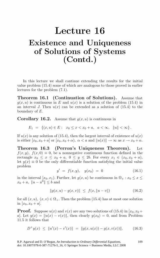
Lecture 16Existence and Uniquenessof Solutions of Systems
(Contd.)
In this lecture we shall continue extending the results for the initialvalue problem (15.4) some of which are analogous to those proved in earlierlectures for the problem (7.1).
Theorem 16.1 (Continuation of Solutions). Assume thatg(x, u) is continuous in E and u(x) is a solution of the problem (15.4) inan interval J. Then u(x) can be extended as a solution of (15.4) to theboundary of E.
Corollary 16.2. Assume that g(x, u) is continuous in
E1 = (x, u) ∈ E : x0 ≤ x < x0 + a, a < ∞, ‖u‖ < ∞ .
If u(x) is any solution of (15.4), then the largest interval of existence of u(x)is either [x0, x0 + a] or [x0, x0 +α), α < a and ‖u(x)‖ → ∞ as x → x0 +α.
Theorem 16.3 (Perron’s Uniqueness Theorem). Letf(x, y), f(x, 0) ≡ 0, be a nonnegative continuous function defined in therectangle x0 ≤ x ≤ x0 + a, 0 ≤ y ≤ 2b. For every x1 ∈ (x0, x0 + a),let y(x) ≡ 0 be the only differentiable function satisfying the initial valueproblem
y′ = f(x, y), y(x0) = 0 (16.1)
in the interval [x0, x1). Further, let g(x, u) be continuous in Ω+ : x0 ≤ x ≤x0 + a, ‖u− u0‖ ≤ b and
‖g(x, u) − g(x, v)‖ ≤ f(x, ‖u− v‖) (16.2)
for all (x, u), (x, v) ∈ Ω+. Then the problem (15.4) has at most one solutionin [x0, x0 + a].
Proof. Suppose u(x) and v(x) are any two solutions of (15.4) in [x0, x0+a]. Let y(x) = ‖u(x) − v(x)‖, then clearly y(x0) = 0, and from Problem11.5 it follows that
D+y(x) ≤ ‖u′(x) − v′(x)‖ = ‖g(x, u(x)) − g(x, v(x))‖. (16.3)
R.P. Agarwal and D. O’Regan, An Introduction to Ordinary Differential Equations,
doi: 10.1007/978-0-387-71276-5_16, © Springer Science + Business Media, LLC 2008
109

110 Lecture 16
Using inequality (16.2) in (16.3), we obtainD+y(x) ≤ f(x, y(x)). Therefore,from Theorem 11.6 it follows that y(x) ≤ r(x), x ∈ [x0, x1) for any x1 ∈(x0, x0 + a), where r(x) is the maximal solution of (16.1). However, fromthe hypothesis r(x) ≡ 0, and hence y(x) ≡ 0 in [x0, x1). This proves thetheorem.
In Theorem 16.3 the function f(x, y) = h(x)y, where h(x) ≥ 0 is contin-uous in [x0, x0 + a] is admissible, i.e., it includes the Lipschitz uniquenesscriterion.
For our next result we need the following lemma.
Lemma 16.4. Let f(x, y) be a nonnegative continuous function forx0 < x ≤ x0 + a, 0 ≤ y ≤ 2b with the property that the only solution y(x)of the DE y′ = f(x, y) in any interval (x0, x1) where x1 ∈ (x0, x0 + a) forwhich y′
+(x0) exists, and
y(x0) = y′+(x0) = 0 (16.4)
is y(x) ≡ 0. Further, let f1(x, y) be a nonnegative continuous function forx0 ≤ x ≤ x0 + a, 0 ≤ y ≤ 2b, f1(x, 0) ≡ 0 and
f1(x, y) ≤ f(x, y), x = x0. (16.5)
Then for every x1 ∈ (x0, x0+a), y1(x) ≡ 0 is the only differentiable functionin [x0, x1), which satisfies
y′1 = f1(x, y1), y1(x0) = 0. (16.6)
Proof. Let r(x) be the maximal solution of (16.6) in [x0, x1). Sincef1(x, 0) ≡ 0, y1(x) ≡ 0 is a solution of the problem (16.6). Thus, r(x) ≥ 0in [x0, x1). Hence, it suffices to show that r(x) = 0 in [x0, x1). Suppose, onthe contrary, that there exists a x2, x0 < x2 < x1 such that r(x2) > 0.Then because of the inequality (16.5), we have
r′(x) ≤ f(x, r(x)), x0 < x ≤ x2.
If ρ(x) is the minimal solution of
y′ = f(x, y), y(x2) = r(x2),
then an application of Problem 11.6 implies that
ρ(x) ≤ r(x) (16.7)
as long as ρ(x) exists to the left of x2. The solution ρ(x) can be continuedto x = x0. If ρ(x3) = 0, for some x3, x0 < x3 < x2, we can affect the con-tinuation by defining ρ(x) = 0 for x0 < x < x3. Otherwise, (16.7) ensures

Existence and Uniqueness of Solutions of Systems (Contd.) 111
the possibility of continuation. Since r(x0) = 0, limx→x+0ρ(x) = 0, and we
define ρ(x0) = 0. Furthermore, since f1(x, y) is continuous at (x0, 0) andf1(x0, 0) = 0, r′
+(x0) exists and is equal to zero. This, because of (16.7), im-plies that ρ′
+(x0) exists and ρ′+(x0) = 0. Thus, ρ′(x) = f(x, ρ(x)), ρ(x0) =
0, ρ′+(x0) = 0, and hence from the hypothesis on f(x, y) it follows that
ρ(x) ≡ 0. This contradicts the assumption that ρ(x2) = r(x2) > 0. There-fore, r(x) ≡ 0.
Theorem 16.5 (Kamke’s Uniqueness Theorem). Letf(x, y) be as in Lemma 16.4, and g(x, u) as in Theorem 16.3, except thatthe condition (16.2) holds for all (x, u), (x, v) ∈ Ω+, x = x0. Then theproblem (15.4) has at most one solution in [x0, x0 + a].
Proof. Define the function
fg(x, y) = sup‖u−v‖=y
‖g(x, u) − g(x, v)‖ (16.8)
for x0 ≤ x ≤ x0 + a, 0 ≤ y ≤ 2b. Since g(x, u) is continuous in Ω+, thefunction fg(x, y) is continuous for x0 ≤ x ≤ x0 + a, 0 ≤ y ≤ 2b. From(16.8) it is clear that the condition (16.2) holds for the function fg(x, y).Moreover, fg(x, y) ≤ f(x, y) for x0 < x ≤ x0 + a, 0 ≤ y ≤ 2b. Lemma 16.4is now applicable with f1(x, y) = fg(x, y) and therefore fg(x, y) satisfies theassumptions of Theorem 16.3. This completes the proof.
Kamke’s uniqueness theorem is evidently more general than that of Per-ron and it includes as special cases many known criteria, e.g., the following:
1. Osgood’s criterion in the interval [x0, x0 + a] : f(x, y) = w(y), wherethe function w(y) is as in Lemma 10.3.2. Nagumo’s criterion in the interval [x0, x0 + a] : f(x, y) = ky/(x− x0),k ≤ 1.3. Krasnoselski–Krein criterion in the interval [x0, x0 + a] :
f(x, y) = min
ky
x− x0, Cyα
, C > 0, 0 < α < 1, k(1 − α) < 1.
Theorem 16.6 (Continuous Dependence on Initial Con-ditions). Let the following conditions hold:
(i) g(x, u) is continuous and bounded by M in a domain E containingthe points (x0, u
0) and (x1, u1).
(ii) g(x, u) satisfies a uniform Lipschitz condition (15.5) in E.(iii) h(x, u) is continuous and bounded by M1 in E.(iv) u(x) and v(x) are the solutions of the initial value problems (15.4)and
v′ = g(x, v) + h(x, v), v(x1) = u1,

112 Lecture 16
respectively, which exist in an interval J containing x0 and x1.
Then for all x ∈ J , the following inequality holds:
‖u(x) − v(x)‖ ≤(
‖u0 − u1‖ + (M +M1)|x1 − x0| +1LM1
)
× exp (L|x− x0|) − 1LM1.
Theorem 16.7 (Differentiation with Respect to InitialConditions). Let the following conditions be satisfied:
(i) g(x, u) is continuous and bounded by M in a domain E containingthe point (x0, u
0).(ii) The matrix ∂g(x, u)/∂u exists and is continuous and bounded by Lin E.(iii) The solution u(x, x0, u
0) of the initial value problem (15.4) exists inan interval J containing x0.
Then the following hold:
1. The solution u(x, x0, u0) is differentiable with respect to u0, and for each
j (1 ≤ j ≤ n), vj(x) = ∂u(x, x0, u0)/∂u0
j is the solution of the initial valueproblem
v′ =∂g
∂u(x, u(x, x0, u
0))v (16.9)
v(x0) = ej = (0, . . . , 0, 1, 0, . . . , 0). (16.10)
2. The solution u(x, x0, u0) is differentiable with respect to x0 and v(x) =
∂u(x, x0, u0)/∂x0 is the solution of the differential system (16.9), satisfying
the initial conditionv(x0) = − g(x0, u
0). (16.11)
Finally, in this lecture we shall consider the differential system
u′ = g(x, u, λ), (16.12)
where λ = (λ1, . . . , λm) ∈ IRm is a parameter.
If in (16.12) we treat λ1, . . . , λm as new variables, then
dλi
dx= 0, 1 ≤ i ≤ m. (16.13)
Thus, the new system consisting of (16.12) and (16.13) is exactly of theform (15.1), but instead of n, now it is (n+m)-dimensional. Hence, for theinitial value problem
u′ = g(x, u, λ), u(x0) = u0, (16.14)

Existence and Uniqueness of Solutions of Systems (Contd.) 113
the result analogous to Theorem 12.4 can be stated as follows.
Theorem 16.8. Let the following conditions be satisfied:
(i) g(x, u, λ) is continuous and bounded by M in a domain E ⊂ IRn+m+1
containing the point (x0, u0, λ0).
(ii) The matrix ∂g(x, u, λ)/∂u exists and is continuous and bounded by Lin E.(iii) The n×m matrix ∂g(x, u, λ)/∂λ exists and is continuous and boundedby L1 in E.
Then the following hold:
1. There exist positive numbers h and ε such that for any λ satisfying‖λ− λ0‖ ≤ ε, there exists a unique solution u(x, λ) of the problem (16.14)in the interval |x− x0| ≤ h.
2. For all λi such that ‖λi − λ0‖ ≤ ε, i = 1, 2, and x in |x − x0| ≤ h thefollowing inequality holds:
‖u(x, λ1) − u(x, λ2)‖ ≤ L1
L‖λ1 − λ2‖(exp(L|x− x0|) − 1).
3. The solution u(x, λ) is differentiable with respect to λ and for eachj (1 ≤ j ≤ m), vj(x, λ) = ∂u(x, λ)/∂λj is the solution of the initial valueproblem
v′(x, λ) =∂g
∂u(x, u(x, λ), λ)v(x, λ) +
∂g
∂λj(x, u(x, λ), λ) (16.15)
v(x0, λ) = 0. (16.16)
Problems
16.1. Solve the following problems by using Picard’s method of succes-sive approximations:
(i) u′ =[
0 1−1 0
]u, u(0) =
[01
].
(ii) u′ =[
0 11 0
]u+
[xx
], u(0) =
[2
−2
].
16.2. Show that the problem (1.6), (1.8) is equivalent to the integralequation
y(x) =n−1∑i=0
(x−x0)i
i!yi+
1(n−1)!
∫ x
x0
(x−t)n−1f(t, y(t), y′(t), . . . , y(n−1)(t))dt.

114 Lecture 16
16.3. Let the following conditions hold:
(i) f(x, φ0, . . . , φn−1) is continuous in
Ω1 : |x− x0| ≤ a,
n−1∑i=0
|φi − yi| ≤ b
and hence there exists a M > 0 such that supΩ1|f(x, φ0, . . . , φn−1)| ≤ M .
(ii) f(x, φ0, . . . , φn−1) satisfies a uniform Lipschitz condition in Ω1, i.e.,for all (x, φ0, . . . , φn−1), (x, ψ0, . . . , ψn−1) ∈ Ω1 there exists a constant Lsuch that
|f(x, φ0, . . . , φn−1) − f(x, ψ0, . . . , ψn−1)| ≤ L
n−1∑i=0
|φi − ψi|.
Show that the problem (1.6), (1.8) has a unique solution in the intervalJh : |x− x0| ≤ h = mina, b/M1, where M1 = M + b+
∑n−1i=0 |yi|.
16.4. Let y(x) and z(x) be two solutions of the DE
y(n) + p1(x)y(n−1) + · · · + pn(x)y = r(x) (16.17)
in the interval J containing the point x0. Show that for all x in J
u(x0) exp(−2K|x− x0|) ≤ u(x) ≤ u(x0) exp(2K|x− x0|),where
K = 1 +n∑
i=1
supx∈J
|pi(x)| and u(x) =n−1∑i=0
(y(i)(x) − z(i)(x))2.
∗16.5. Consider the initial value problem
y′′ + α(y, y′)y′ + β(y) = f(x), y(0) = y0, y′(0) = y1
where α(y, y′), β(y) are continuous together with their first-order partialderivatives, and f(x) is continuous and bounded on IR, α ≥ 0, yβ(y) ≥0. Show that this problem has a unique solution and it can be extendedto [0,∞).
16.6. Using an example of the form
u′1 = u2u′
2 = −u1
observe that a generalization of Theorem 11.1 to systems of first-order DEswith inequalities interpreted component-wise is in general not true.

Existence and Uniqueness of Solutions of Systems (Contd.) 115
Answers or Hints
16.1. (i) (sinx, cosx)T . (ii) (ex + 2e−x − x− 1, ex − 2e−x − x− 1)T .
16.2. Use Taylor’s formula.
16.3. Write (1.6), (1.8) in system form and then apply Theorem 15.2.
16.4. Use the inequality 2|a||b| ≤ a2 + b2 to get −2Ku(x) ≤ u′(x) ≤2Ku(x).
16.6. Let J = [0, π), u(x) = (sinx, cosx)T and v(x) = (−ε, 1 − ε)T , 0 <ε < 1.

Lecture 17General Propertiesof Linear Systems
If the system (15.1) is linear, i.e.,
gi(x, u) = ai1(x)u1 + ai2(x)u2 + · · · + ain(x)un + bi(x), 1 ≤ i ≤ n,
then it can be written as
u′ = A(x)u+ b(x), (17.1)
where A(x) is an n × n matrix with elements aij(x), b(x) is an n × 1vector with components bi(x), and u(x) is an n × 1 unknown vector withcomponents ui(x).
The existence and uniqueness of solutions of the differential system(17.1) together with the initial condition
u(x0) = u0 (17.2)
in an interval J containing x0 follows from Corollary 15.4 provided thefunctions aij(x), bi(x), 1 ≤ i, j ≤ n are continuous in J which we shallassume throughout.
The principle of superposition for the first-order linear DEs given inProblem 5.2 holds for the differential system (17.1) also, and it is stated asfollows: If u(x) is a solution of the differential system u′ = A(x)u + b1(x)and v(x) is a solution of v′ = A(x)v + b2(x), then φ(x) = c1u(x) + c2v(x)is a solution of the differential system φ′ = A(x)φ+ c1b
1(x) + c2b2(x). For
this, we have
φ′(x) = c1u′(x) + c2v
′(x)
= c1(A(x)u(x) + b1(x)) + c2(A(x)v(x) + b2(x))
= A(x)(c1u(x) + c2v(x)) + c1b1(x) + c2b
2(x)
= A(x)φ(x) + c1b1(x) + c2b
2(x).
In particular, if b1(x) = b2(x) ≡ 0, i.e., u(x) and v(x) are solutions ofthe homogeneous differential system
u′ = A(x)u, (17.3)
R.P. Agarwal and D. O’Regan, An Introduction to Ordinary Differential Equations,
116doi: 10.1007/978-0-387-71276-5_17, © Springer Science + Business Media, LLC 2008

General Properties of Linear Systems 117
then c1u(x) + c2v(x) is also a solution. Thus, solutions of the homoge-neous differential system (17.3) form a vector space. Further, if b1(x) =b2(x), c1 = 1, c2 = −1 and u(x) is a solution of (17.1), then v(x) is also asolution of (17.1) if and only if u(x)−v(x) is a solution of (17.3). Thus, thegeneral solution of (17.1) is obtained by adding to a particular solution of(17.1) the general solution of the corresponding homogeneous system (17.3).
To find the dimension of the vector space of the solutions of (17.3) weneed to define the concept of linear independence and dependence of vector-valued functions. The vector-valued functions u1(x), . . . , um(x) defined inan interval J are said to be linearly independent in J, if the relation c1u1(x)+· · ·+cmum(x) = 0 for all x in J implies that c1 = · · · = cm = 0. Conversely,these functions are said to be linearly dependent if there exist constantsc1, . . . , cm not all zero such that c1u1(x) + · · · + cmu
m(x) = 0 for all x ∈ J.
Let m functions u1(x), . . . , um(x) be linearly dependent in J and ck = 0;then we have
uk(x) = − c1cku1(x) − · · · − ck−1
ckuk−1(x) − ck+1
ckuk+1(x) − · · · − cm
ckum(x),
i.e., uk(x) (and hence at least one of these functions) can be expressed as alinear combination of the remaining m− 1 functions. On the other hand, ifone of these functions, say, uk(x), is a linear combination of the remainingm− 1 functions, so that
uk(x) = c1u1(x) + · · · + ck−1u
k−1(x) + ck+1uk+1(x) + · · · + cmu
m(x),
then obviously these functions are linearly dependent. Hence, if two func-tions are linearly dependent in J, then each one of these functions is iden-tically equal to a constant times the other function, while if two functionsare linearly independent, then it is impossible to express either function asa constant times the other. The concept of linear independence allows usto distinguish when the given functions are “essentially” different.
Example 17.1. (i) The functions 1, x, . . . , xm−1 are linearly inde-pendent in every interval J. For this, c1 + c2x + · · · + cmx
m−1 ≡ 0 in Jimplies that c1 = · · · = cm = 0. If any ck were not zero, then the equationc1 + c2x + · · · + cmx
m−1 = 0 could hold for at most m − 1 values of x,whereas it must hold for all x in J.
(ii) The functions
u1(x) =
[ex
ex
], u2(x) =
[e2x
3e2x
]
are linearly independent in every interval J. Indeed,
c1
[ex
ex
]+ c2
[e2x
3e2x
]= 0

118 Lecture 17
implies that c1ex + c2e2x = 0 and c1ex + 3c2e2x = 0, which is possible only
for c1 = c2 = 0.
(iii) The functions
u1(x) =
[sinx
cosx
], u2(x) =
[0
0
]
are linearly dependent.
For the given n vector-valued functions u1(x), . . . , un(x) the determi-nant W (u1, . . . , un)(x) or W (x), when there is no ambiguity, defined by∣∣∣∣∣∣∣∣∣∣∣
u11(x) · · · un
1 (x)
u12(x) · · · un
2 (x)
· · ·u1
n(x) · · · unn(x)
∣∣∣∣∣∣∣∣∣∣∣is called the Wronskian of these functions. This determinant is closelyrelated to the question of whether u1(x), . . . , un(x) are linearly independent.In fact, we have the following result.
Theorem 17.1. If the Wronskian W (x) of n vector-valued functionsu1(x), . . . , un(x) is different from zero for at least one point in an intervalJ ; then these functions are linearly independent in J.
Proof. Let u1(x), . . . , un(x) be linearly dependent in J, then there existn constants c1, . . . , cn not all zero such that
∑ni=1 ciu
i(x) = 0 in J. This isthe same as saying the homogeneous system of equations
∑ni=1 u
ik(x)ci =
0, 1 ≤ k ≤ n, x ∈ J, has a nontrivial solution. However, from Theorem13.2 this homogeneous system for each x ∈ J has a nontrivial solution ifand only if W (x) = 0. But W (x) = 0 for at least one x in J, and, thereforeu1(x), . . . , un(x) cannot be linearly dependent.
In general the converse of this theorem is not true. For instance, for
u1(x) =
[x
1
], u2(x) =
[x2
x
],
which are linearly independent in any interval J, W (u1, u2)(x) = 0 in J.This example also shows that W (u1, u2)(x) = 0 in J is not necessary forthe linear independence of u1(x) and u2(x) in J, and W (u1, u2)(x) = 0 inJ may not imply that u1(x) and u2(x) are linearly dependent in J. Thus,the only conclusion we have is W (x) = 0 in J implies that u1(x), . . . , un(x)are linearly independent in J , and linear dependence of these functions inJ implies that W (x) = 0 in J.

General Properties of Linear Systems 119
The converse of Theorem 17.1 holds if u1(x), . . . , un(x) are the solutionsof the homogeneous differential system (17.3) in J. This we shall prove inthe following theorem.
Theorem 17.2. Let u1(x), . . . , un(x) be linearly independent solutionsof the differential system (17.3) in J. Then W (x) = 0 for all x ∈ J.
Proof. Let x0 be a point in J where W (x0) = 0, then from Theorem 13.2there exist constants c1, . . . , cn not all zero such that
∑ni=1 ciu
i(x0) = 0.Since u(x) =
∑ni=1 ciu
i(x) is a solution of (17.3), and u(x0) = 0, from theuniqueness of the solutions it follows that u(x) =
∑ni=1 ciu
i(x) = 0 in J.However, the functions u1(x), . . . , un(x) are linearly independent in J so wemust have c1 = · · · = cn = 0. This contradiction completes the proof.
Thus, on combining the results of Theorems 17.1 and 17.2 we find thatthe solutions u1(x), . . . , un(x) of the differential system (17.3) are linearlyindependent in J if and only if there exists at least one point x0 ∈ J suchthatW (x0) = 0, i.e, the vectors u1(x0), . . . , un(x0) are linearly independent.Hence, the solutions u1(x), . . . , un(x) of the system (17.3) satisfying theinitial conditions
ui(x0) = ei, i = 1, . . . , n (17.4)
are linearly independent in J. This proves the existence of n linearly inde-pendent solutions of the differential system (17.3) in J.
Now let u(x) be any solution of the differential system (17.3) in Jsuch that u(x0) = u0. Then from the existence and uniqueness of thesolutions of the initial value problem (17.3), (17.2) it is immediate thatu(x) =
∑ni=1 u
0i u
i(x), where ui(x) is the solution of the problem (17.3),(17.4). Thus, every solution of (17.3) can be expressed as a linear combina-tion of the n linearly independent solutions of (17.3), (17.4). In conclusion,we find that the vector space of all solutions of (17.3) is of dimension n.
Finally, in this lecture we shall prove the following result, which gives arelation between the Wronskian W (x) and the matrix A(x).
Theorem 17.3 (Abel’s Formula). Let u1(x), . . . , un(x) be thesolutions of the differential system (17.3) in J and x0 ∈ J. Then for allx ∈ J ,
W (x) = W (x0) exp(∫ x
x0
TrA(t)dt). (17.5)
Proof. In view of (13.5) the derivative of the Wronskian W (x) can bewritten as
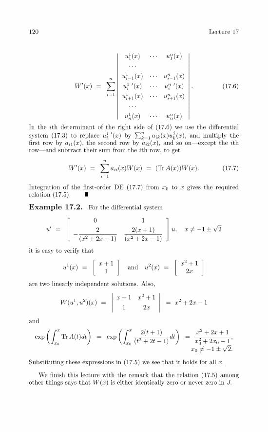
120 Lecture 17
W ′(x) =n∑
i=1
∣∣∣∣∣∣∣∣∣∣∣∣∣∣∣∣∣
u11(x) · · · un
1 (x)
· · ·u1
i−1(x) · · · uni−1(x)
u1 ′i (x) · · · un ′
i (x)
u1i+1(x) · · · un
i+1(x)
· · ·u1
n(x) · · · unn(x)
∣∣∣∣∣∣∣∣∣∣∣∣∣∣∣∣∣
. (17.6)
In the ith determinant of the right side of (17.6) we use the differentialsystem (17.3) to replace uj ′
i (x) by∑n
k=1 aik(x)ujk(x), and multiply the
first row by ai1(x), the second row by ai2(x), and so on—except the ithrow—and subtract their sum from the ith row, to get
W ′(x) =n∑
i=1
aii(x)W (x) = (TrA(x))W (x). (17.7)
Integration of the first-order DE (17.7) from x0 to x gives the requiredrelation (17.5).
Example 17.2. For the differential system
u′ =
⎡⎣ 0 1
− 2(x2 + 2x− 1)
2(x+ 1)(x2 + 2x− 1)
⎤⎦u, x = −1 ±
√2
it is easy to verify that
u1(x) =[x+ 1
1
]and u2(x) =
[x2 + 1
2x
]
are two linearly independent solutions. Also,
W (u1, u2)(x) =
∣∣∣∣∣ x+ 1 x2 + 1
1 2x
∣∣∣∣∣ = x2 + 2x− 1
and
exp(∫ x
x0
TrA(t)dt)
= exp(∫ x
x0
2(t+ 1)(t2 + 2t− 1)
dt
)=
x2 + 2x+ 1x2
0 + 2x0 − 1,
x0 = −1 ± √2.
Substituting these expressions in (17.5) we see that it holds for all x.
We finish this lecture with the remark that the relation (17.5) amongother things says that W (x) is either identically zero or never zero in J.

General Properties of Linear Systems 121
Problems
17.1. Show that the linear differential system (17.1) remains linearafter the change of the independent variable x = p(t).
17.2. Matrices of the form⎡⎢⎢⎢⎢⎣
0 1 0 · · · 00 0 1 · · · 0
· · ·0 0 0 · · · 1
−pn −pn−1 −pn−2 · · · −p1
⎤⎥⎥⎥⎥⎦
are called companion matrices. Show the following:
(i) If y(x) satisfies the nth-order linear homogeneous DE
y(n) + p1(x)y(n−1) + · · · + pn(x)y = 0 (17.8)
and if the vector-valued function u(x) is defined by ui(x) = y(i−1)(x), i =1, 2, . . . , n, then u′ = A(x)u with A(x) in the companion form.
(ii) If yk(x), 1 ≤ k ≤ n are n solutions of (17.8), then
uk(x) = (yk(x), y′k(x), . . . , y(n−1)
k (x))T , 1 ≤ k ≤ n
satisfy the system u′ = A(x)u.
(iii) W (u1, . . . , un)(x) = W (u1, . . . , un)(x0) exp(
−∫ x
x0
p1(t)dt).
17.3. The Wronskian of n functions y1(x), . . . , yn(x) which are (n− 1)times differentiable in an interval J is defined by the determinant
W (y1, . . . , yn)(x) =
∣∣∣∣∣∣∣∣∣∣
y1(x) · · · yn(x)
y′1(x) · · · y′
n(x)
· · ·y(n−1)1 (x) · · · y
(n−1)n (x)
∣∣∣∣∣∣∣∣∣∣.
Show the following:
(i) If W (y1, . . . , yn)(x) is different from zero for at least one point in J,then the functions y1(x), . . . , yn(x) are linearly independent in J .(ii) If the functions y1(x), . . . , yn(x) are linearly dependent in J, then theWronskian W (y1, . . . , yn)(x) = 0 in J .(iii) The converse of (i) as well as of (ii) is not necessarily true.

122 Lecture 17
(iv) If W (y1, . . . , yn)(x) = 0 in J, but for some set of (n − 1), y’s (say,without loss of generality, all but yn(x)) W (y1, . . . , yn−1)(x) = 0 for allx ∈ J, then the functions y1(x), . . . , yn(x) are linearly dependent in J.
17.4. Let y1(x), . . . , yn(x) be n times continuously differentiable func-tions in an interval J and W (y1, . . . , yn)(x) = 0. Show that
W (y1, . . . , yn, y)(x)W (y1, . . . , yn)(x)
= 0
is an nth-order linear homogeneous DE for which y1(x), . . . , yn(x) are so-lutions.
17.5. Show that the DE (17.8) can be transformed to its normal form
z(n) + q2(x)z(n−2) + q3(x)z(n−3) + · · · + qn(x)z = 0,
where
z(x) = y(x) exp(
1n
∫ x
p1(t)dt),
provided p1(x) is (n− 1) times differentiable in J. In particular for n = 2,the normal form of (17.8) is
z′′ +(p2(x) − 1
2p′1(x) − 1
4p21(x)
)z = 0.
17.6. Let φ1(x) = 0 in J be a solution of the DE (17.8). If v2, . . . , vn
are linearly independent solutions of the DE
φ1v(n−1) + · · · + [nφ(n−1)
1 + p1(x)(n− 1)φ(n−2)1 + · · · + pn−1(x)φ1]v = 0
and if vk = u′k, k = 2, . . . , n, then φ1, u2φ1, . . . , unφ1 are linearly indepen-
dent solutions of (17.8) in J. In particular, for n = 2 the second linearlyindependent solution of (17.8) is given by
φ2(x) = φ1(x)∫ x
x0
1(φ1(t))2
exp(
−∫ t
x0
p1(s)ds)dt
(see (6.5)).
17.7. Let u(x), v(x) and w(x) be the solutions of the DE y′′′ + y = 0satisfying u(0) = 1, u′(0) = 0, u′′(0) = 0; v(0) = 0, v′(0) = 1, v′′(0) = 0;w(0) = 0, w′(0) = 0, w′′(0) = 1. Without solving the DE, show thefollowing:
(i) u′(x) = −w(x).(ii) v′(x) = u(x).

General Properties of Linear Systems 123
(iii) w′(x) = v(x).(iv) W (u, v, w) = u3 − v3 + w3 + 3uvw = 1.
Answers or Hints
17.1. For each k, 0 ≤ k ≤ n it is easy to find
dkydxk =
∑ki=0 pki(t)diy
dti ,
where pki(t) are some suitable functions.
17.2. To show (i) and (ii) write the equation (17.8) in a system form.part (iii) follows from Abel’s formula (17.5).
17.3. (i) If yi(x), 1 ≤ i ≤ n are linearly dependent, then there exist non-trivial ci, 1 ≤ i ≤ n such that
∑ni=1 ciyi(x) = 0 for all x ∈ J. Differentiating
this, we obtain∑n
i=1 ciy(k)i (x) = 0, k = 0, 1, . . . , n − 1 for all x ∈ J. But,
this implies W (x) = 0. (ii) Clear from part (i). (iii) Consider the functionsy1(x) = x3, y2(x) = x2|x|. (iv) W (y1, . . . , yn−1, y)(x) = 0 is a linear homo-geneous DE such that the coefficient of y(n−1)(x) isW (y1, . . . , yn−1)(x) = 0.For this (n− 1)th-order DE there are n solutions yi(x), 1 ≤ i ≤ n.
17.4. See part (iv) of Problem 17.3.
17.5. Use Leibnitz’s formula.
17.6. Since φ1(x) is a solution of the DE (17.8), y = uφ1 will also beits solution provided 0 = (uφ1)(n) + p1(x)(uφ1)(n−1) + · · · + pn(x)(uφ1) =φ1v
(n−1) + (nφ′1 + p1(x)φ1)v(n−2) + · · · + (nφ(n−1)
1 + (n− 1)p1(x)φ(n−2)1 +
· · ·+pn−1(x)φ1)v, where v = u′. The coefficient of v(n−1) is φ1, and hence ifφ1(x) = 0 in J , then the above (n−1)th-order DE has n−1 linearly indepen-dent solutions v2, . . . , vn in J. If x0 ∈ J, and uk(x) =
∫ x
x0vk(t)dt, 2 ≤ k ≤ n
then the functions φ1, u2φ1, . . . , unφ1 are solutions of (17.8). To show thatthese solutions are linearly independent, let c1φ1+c2u2φ1+· · ·+cnunφ1 = 0,where not all c1, . . . , cn are zero. However, since φ1 = 0 in J, this im-plies that c1 + c2u2 + · · · + cnun = 0, and on differentiation we obtainc2u
′2 + · · · + cnu
′n = 0, i.e., c2v2 + · · · + cnvn = 0. Since v2, . . . , vn are
linearly independent c2 = · · · = cn = 0, which in turn also imply thatc1 = 0.
17.7. Since W (u, v, w)(0) = 1, u, v, w are linearly independent solutions ofy′′′ + y = 0. Now since (u′)′′′ + (u′) = 0, u′ is also a solution of y′′′ + y = 0.Hence, there exist nonzero constants c1, c2, c3 such that u′(x) = c1u(x) +c2v(x) + c3w(x). Part (iv) follows from parts (i)–(iii) and Abel’s formula.

Lecture 18Fundamental Matrix Solution
In our previous lecture we have seen that any solution u(x) of the dif-ferential system (17.3) satisfying u(x0) = u0 can be written as u(x) =∑n
i=1 u0iu
i(x), where ui(x) is the solution of the initial value problem (17.3),(17.4). In matrix notation this solution can be written as u(x) = Φ(x, x0)u0,where Φ(x, x0) is an n × n matrix whose ith column is ui(x). The matrixΦ(x, x0) is called the principal fundamental matrix ; however, some authorsprefer to call it evolution or transition matrix. It is easy to verify thatΦ(x, x0) is a solution of the matrix initial value problem
dΦdx
= A(x)Φ, Φ(x0) = I. (18.1)
The fact that the initial value problem (18.1) has a unique solutionΦ(x, x0) in J can be proved exactly as for the problem (17.1), (17.2). More-over, the iterative scheme
Φm+1(x) = I +∫ x
x0
A(t)Φm(t)dt, m = 0, 1, . . . (18.2)
Φ0(x) = I (18.3)
converges to Φ(x, x0), and
Φ(x, x0) = I +∫ x
x0
A(t)dt+∫ x
x0
∫ t
x0
A(t)A(t1)dt1dt+ · · · . (18.4)
The series (18.4) is called Peano–Baker series for the solution of (18.1). IfA is an n× n constant matrix, then it can be taken out from the integralsand (18.4) becomes
Φ(x, x0) = I +A
∫ x
x0
dt+A2∫ x
x0
∫ t
x0
dt1dt+ · · ·
= I +∞∑
m=1
[A(x− x0)]m
m!= exp(A(x− x0)).
Summarizing this discussion, specifically we have proved the followingtheorem.
R.P. Agarwal and D. O’Regan, An Introduction to Ordinary Differential Equations,
124doi: 10.1007/978-0-387-71276-5_18, © Springer Science + Business Media, LLC 2008

Fundamental Matrix Solution 125
Theorem 18.1. The matrix
Φ(x, x0) = exp(A(x− x0)) (18.5)
is the principal fundamental matrix of the system
u′ = Au, (18.6)
where A is a constant matrix.
Example 18.1. For the matrix A =[
0 1−1 0
]it is easily seen that
A4m+1 = A, A4m+2 = −I, A4m+3 = −A, A4m+4 = I for m = 0, 1, . . . andhence the series (18.4) can be summed, to obtain[
cos(x− x0) sin(x− x0)
− sin(x− x0) cos(x− x0)
].
In our previous lecture we have also proved that the solutions u1(x), . . . ,un(x) of the differential system (17.3) are linearly independent in J if andonly if there exists at least one point x0 ∈ J such that W (x0) = 0. If thesesolutions are linearly independent, then the set u1(x), . . . , un(x) is calleda fundamental system of solutions of (17.3). Further, the n × n matrixΨ(x) = [u1(x), . . . , un(x)] is called the fundamental matrix of (17.3). Forthis matrix Ψ(x), we shall prove the following result.
Theorem 18.2. If Ψ(x) is a fundamental matrix of the differentialsystem (17.3), then for any constant nonsingular n × n matrix C, Ψ(x)Cis also a fundamental matrix of (17.3), and every fundamental matrix of(17.3) is of the form Ψ(x)C for some constant nonsingular n× n matrix C.
Proof. Obviously, Ψ′(x) = A(x)Ψ(x), and hence Ψ′(x)C = A(x)Ψ(x)C,which is the same as (Ψ(x)C)′ = A(x)(Ψ(x)C), i.e., Ψ(x) and Ψ(x)C bothare solutions of the same matrix differential system Φ′ = A(x)Φ. Further,since det Ψ(x) = 0 and detC = 0 it follows that det (Ψ(x)C) = 0, andhence Ψ(x)C is also a fundamental matrix solution of (17.3). Conversely,let Ψ1(x) and Ψ2(x) be two fundamental matrix solutions of (17.3). IfΨ−1
2 (x)Ψ1(x) = C(x), i.e., Ψ1(x) = Ψ2(x)C(x), then we find that Ψ′1(x) =
Ψ′2(x)C(x) + Ψ2(x)C ′(x) which is the same as
A(x)Ψ1(x) = A(x)Ψ2(x)C(x)+Ψ2(x)C ′(x) = A(x)Ψ1(x)+Ψ2(x)C ′(x);
i.e., Ψ2(x)C ′(x) = 0, or C ′(x) = 0, and hence C(x) is a constant matrix.Further, since both Ψ1(x) and Ψ2(x) are nonsingular, this constant matrixis also nonsingular.
As a consequence of this theorem, we find
Φ(x, x0) = Ψ(x)Ψ−1(x0) (18.7)

126 Lecture 18
and the solution of the initial value problem (17.3), (17.2) can be written as
u(x) = Ψ(x)Ψ−1(x0)u0. (18.8)
Since the product of matrices is not commutative, for a given constantnonsingular matrix C, CΨ(x) need not be a fundamental matrix solution ofthe differential system (17.3). Further, two different homogeneous systemscannot have the same fundamental matrix, i.e., Ψ(x) determines the matrixA(x) in (17.3) uniquely by the relation A(x) = Ψ′(x)Ψ−1(x). However, fromTheorem 18.2 the converse is not true.
Now differentiating the relation Ψ(x)Ψ−1(x) = I, we obtain
Ψ′(x)Ψ−1(x) + Ψ(x)(Ψ−1(x))′ = 0
and hence(Ψ−1(x))′ = − Ψ−1(x)A(x),
which is the same as((Ψ−1(x))T
)′= −AT (x)(Ψ−1(x))T . (18.9)
Therefore, (Ψ−1(x))T is a fundamental matrix of the differential system
u′ = −AT (x)u. (18.10)
The system (18.10) is called the adjoint system to the differential system(17.3). This relationship is symmetric in the sense that (17.3) is the adjointsystem to (18.10) and vice versa.
An important property of adjoint systems is given in the following result.
Theorem 18.3. If Ψ(x) is a fundamental matrix of the differentialsystem (17.3), then χ(x) is a fundamental matrix of its adjoint system(18.10) if and only if
χT (x)Ψ(x) = C, (18.11)
where C is a constant nonsingular n× n matrix.
Proof. If Ψ(x) is a fundamental matrix of the differential system(17.3), then from (18.9) it follows that (Ψ−1(x))T is a fundamental matrixof the differential system (18.10), and hence Theorem 18.2 gives χ(x) =(Ψ−1(x))TD, where D is a constant nonsingular n×n matrix. Thus, on us-ing the fact that (Ψ−1(x))T is a fundamental matrix we have ΨT (x)χ(x) =D, which is the same as χT (x)Ψ(x) = DT . Therefore, (18.11) holds withC = DT . Conversely, if Ψ(x) is a fundamental matrix of (17.3) satisfying(18.11), then we have ΨT (x)χ(x) = CT and hence χ(x) = (ΨT (x))−1CT .Thus, by Theorem 18.2, χ(x) is a fundamental matrix of the adjoint system(18.10).

Fundamental Matrix Solution 127
As a consequence of this theorem, if A(x) = −AT (x), then (ΨT (x))−1
being a fundamental matrix of (18.10) is also a fundamental matrix of thedifferential system (17.3). Thus, Theorem 18.2 gives Ψ(x) = (ΨT (x))−1C,which is the same as ΨT (x)Ψ(x) = C. Hence, in this particular case theEuclidean length of any solution of the differential system (17.3) is a con-stant.
Now we shall show that the method of variation of parameters used inLectures 5 and 6 to find the solutions of nonhomogeneous first and second-order DEs is equally applicable for the nonhomogeneous system (17.1).For this, we seek a vector-valued function v(x) such that Φ(x, x0)v(x) is asolution of the system (17.1). We have
Φ′(x, x0)v(x) + Φ(x, x0)v′(x) = A(x)Φ(x, x0)v(x) + b(x),
which reduces to giveΦ(x, x0)v′(x) = b(x);
and hence from Problem 18.2, it follows that
v′(x) = Φ−1(x, x0)b(x) = Φ(x0, x)b(x).
Thus, the function v(x) can be written as
v(x) = v(x0) +∫ x
x0
Φ(x0, t)b(t)dt.
Finally, since u(x0) = Φ(x0, x0)v(x0) = v(x0), the solution of the initialvalue problem (17.1), (17.2) takes the form
u(x) = Φ(x, x0)u0 + Φ(x, x0)∫ x
x0
Φ(x0, t)b(t)dt, (18.12)
which from Problem 18.2 is the same as
u(x) = Φ(x, x0)u0 +∫ x
x0
Φ(x, t)b(t)dt. (18.13)
If we use the relation (18.7) in (18.12), then it is the same as
u(x) = Ψ(x)c+∫ x
x0
Ψ(x)Ψ−1(t)b(t)dt, (18.14)
where the constant vector c = Ψ−1(x0)u0. Hence, we have an explicit rep-resentation of the general solution of (17.1) in terms of any fundamentalmatrix Ψ(x) of the differential system (17.3).
In the case when A(x) is a constant matrix A, relation (18.5) can beused in (18.13), to obtain
u(x) = eA(x−x0)u0 +∫ x
x0
eA(x−t)b(t)dt. (18.15)

128 Lecture 18
Example 18.2. Consider the system
u′ =[
0 1−2 3
]u+
[11
]. (18.16)
For the corresponding homogeneous system
u′ =[
0 1−2 3
]u
it is easy to verify that the principal fundamental matrix is
Φ(x, 0) =
[2ex − e2x −ex + e2x
2ex − 2e2x −ex + 2e2x
]=
[ex e2x
ex 2e2x
][2 −1
−1 1
].
Thus, the solution of (18.16) satisfying u(0) = u0 can be written as
u(x) =
[ex e2x
ex 2e2x
][2 −1
−1 1
]u0
+
[ex e2x
ex 2e2x
]∫ x
0
[2e−t −e−t
−e−2t e−2t
][1
1
]dt
=
[2ex − e2x −ex + e2x
2ex − 2e2x −ex + 2e2x
]u0 + (ex − 1)
[1
1
].
Problems
18.1. Show that the vector-valued function
u(x) = exp(∫ x
x0
A(t)dt)u0
is not a solution of the differential system (17.3) unless A(x) and∫ x
x0A(t)dt
commute for all x.
18.2. Let Φ(x, x0) be the principal fundamental matrix of the system(17.3) in an interval J. Show that Φ(x, x0) = Φ(x, x1)Φ(x1, x0), where x1 ∈J, and hence, in particular, Φ−1(x, x0) = Φ(x0, x), and Φ(x, x) = I for allx ∈ J.
18.3. For the n × n matrix Φ(x, t) appearing in (18.13), show thefollowing:
(i) ∂Φ(x, t)/∂x = A(x)Φ(x, t).

Fundamental Matrix Solution 129
(ii) ∂Φ(x, t)/∂t = −Φ(x, t)A(t).
(iii) Φ(x, t) = I +∫ x
tA(s)Φ(s, t)ds.
(iv) Φ(x, t) = I +∫ x
tΦ(x, s)A(s)ds.
18.4. Show that a square nonsingular matrix Φ(., .) which depends ontwo arguments and is differentiable with respect to each argument in J is aprincipal fundamental matrix if Φ(x0, x0) = I for all x0 in J and the matrix
[d
dxΦ(x, x0)
]Φ−1(x, x0)
depends on x alone.
18.5. Let Φ(x) = Φ(x, 0) be the principal fundamental matrix of thesystem (18.6). Show the following:
(i) For any real x0,Φ1(x) = Φ(x− x0) is a fundamental matrix.
(ii) Φ(x − x0) = Φ(x)Φ(−x0) = Φ(x)Φ−1(x0), and hence Φ(−x0) =Φ−1(x0).
18.6. The linear differential system (17.3) is said to be self-adjoint whenA(x) = −AT (x) for all x in J. Let Φ(x, x0) be the principal fundamentalmatrix of the system (17.3), and Ψ(x, x0) be the principal fundamentalmatrix of the adjoint system (18.10). Show that the differential system(17.3) is self-adjoint if and only if Φ(x, x0) = ΨT (x0, x).
18.7. Let the matrix A(x) be such that aij(x) ≥ 0 for all i = j and allx ≥ x0. Show the following:
(i) Every element of the principal fundamental matrix Φ(x, x0) of thesystem (17.3) is nonnegative for all x ≥ x0.
(ii) If u(x) and v(x) are two solutions of the differential system (17.3)satisfying ui(x0) ≥ vi(x0), 1 ≤ i ≤ n, then ui(x) ≥ vi(x), 1 ≤ i ≤ n for allx ≥ x0.
18.8. Equations of the form
p0xny(n) + p1x
n−1y(n−1) + · · · + pny = 0, x > 0, p0 = 0 (18.17)
are called Euler’s DEs. Show that there exist u1(x), . . . , un(x) such that thedifferential system (18.17) can be converted to u′(x) = x−1Au(x), where Ais an n× n constant matrix.
18.9. For the given n linearly independent solutions y1(x), . . . , yn(x)

130 Lecture 18
of the homogeneous DE (17.8) in an interval J, we define
H(x, t) =y1(x)∆1(t) + · · · + yn(x)∆n(t)
W (y1, . . . , yn)(t)
=
∣∣∣∣∣∣∣∣∣∣∣∣
y1(t) · · · yn(t)
y′1(t) · · · y′
n(t)
· · ·y(n−2)1 (t) · · · y
(n−2)n (t)
y1(x) · · · yn(x)
∣∣∣∣∣∣∣∣∣∣∣∣
/∣∣∣∣∣∣∣∣∣∣
y1(t) · · · yn(t)
y′1(t) · · · y′
n(t)
· · ·y(n−1)1 (t) · · · y
(n−1)n (t)
∣∣∣∣∣∣∣∣∣∣;
i.e., ∆i(t) is the cofactor of the element y(n−1)i (t) in the Wronskian
W (y1, . . . , yn)(t). Show the following:
(i) H(x, t) is defined for all (x, t) in J × J .(ii) ∂iH(x, t)/∂xi, 0 ≤ i ≤ n, are continuous for all (x, t) in J × J .(iii) For each fixed t in J the function z(x) = H(x, t) is a solution of theDE (17.8) satisfying z(i)(t) = 0, 0 ≤ i ≤ n− 2, z(n−1)(t) = 1.(iv) The function
y(x) =∫ x
x0
H(x, t)r(t)dt
is a particular solution of the nonhomogeneous DE (16.17), satisfyingy(i)(x0) = 0, 0 ≤ i ≤ n− 1.(v) The general solution of (16.17) can be written as
y(x) =n∑
i=1
ciyi(x) +∫ x
x0
H(x, t)r(t)dt,
where ci, 1 ≤ i ≤ n, are arbitrary constants.
18.10. Let v(x) be the solution of the initial value problem
y(n) + p1y(n−1) + · · · + pny = 0
y(i)(0) = 0, 0 ≤ i ≤ n− 2, y(n−1)(0) = 1.(18.18)
Show that the function
y(x) =∫ x
x0
v(x− t)r(t)dt
is the solution of the nonhomogeneous DE
y(n) + p1y(n−1) + · · · + pny = r(x) (18.19)
satisfying y(i)(x0) = 0, 0 ≤ i ≤ n− 1.

Fundamental Matrix Solution 131
18.11. Open-loop input–output control systems can be written in theform
u′ = Au+ by(x), z = cTu+ dy(x),
where the functions y(x), z(x) and the constant d are scalar. Here y(x) isthe known input and z(x) is the unknown output. Show that if u(0) = u0
is known, then
(i) u(x) = eAxu0 +∫ x
0eA(x−t)by(t)dt;
(ii) z(x) = cT eAxu0 + dy(x) +∫ x
0
(cT eA(x−t)b
)y(t)dt.
The function h(t) = cT eAxb is called the impulse response function for thegiven control system.
Answers or Hints
18.1. Expand exp(∫ x
x0A(t)dt
)and then compare u′(x) and A(x)u(x).
18.2. Verify that Ψ(x) = Φ(x, x1)Φ(x1, x0) is a fundamental matrix solu-tion of (18.1). The result now follows from the uniqueness.
18.3. Use Φ(x, t) = Φ(x)Φ−1(t).
18.4.[
ddxΦ(x, x0)
]Φ−1(x, x0) = A(x) is the same as d
dxΦ(x, x0) = A(x)×Φ(x, x0).
18.5. (i) Verify directly. (ii) From Theorem 18.2, Φ(x− x0) = Φ(x)C.
18.6. Use Theorem 18.3 and Problems 18.2 and 18.3.
18.7. (i) If aij(x) ≥ 0, 1 ≤ i, j ≤ n, then the sequence Φm(x) generatedby Φ0(x) = I,
Φm+1(x) = I +∫ x
x0
A(t)Φm(t)dt, m = 0, 1, . . . ,
converges to Φ(x, x0) and obviously each Φm(x) ≥ 0, and hence Φ(x, x0) ≥0 for all x ≥ x0. Now note that (17.3) is the same as
u′i − aii(x)ui =
n∑j = 1j = i
aij(x)uj , 1 ≤ i ≤ n.
(ii) Use the representation u(x) = Φ(x, x0)u(x0).

132 Lecture 18
18.8. For n = 3 let y = u1, xu′1 = u2 so that u′
2 = xu′′1 + u′
1, u′′2 =
xu′′′1 + 2u′′
1 . Next let xu′2 = u3 so that u′
3 = xu′′2 + u′
2 = x(xu′′′1 + 2u′′
1) + u′2
and hence
xu′3 = x3u′′′
1 + 2x2u′′1 + xu′
2 = −p3
p0u1 −
(2 +
p2 − p1
p0
)u2 +
(3 − p1
p0
)u3.
Now write these equations in the required system form.
18.9. Verify directly.
18.10. For each fixed t, z(x) = v(x− t) is also a solution of (18.18) satis-fying z(i)(t) = 0, 0 ≤ i ≤ n− 2, z(n−1)(t) = 1. Now use Problem 18.9(iv).
18.11. Use (18.15).

Lecture 19Systems with
Constant Coefficients
Our discussion in Lecture 18 has restricted usage of obtaining explicitsolutions of homogeneous and, in general, of nonhomogeneous differentialsystems. This is so because the solution (18.4) involves an infinite serieswith repeated integrations and (18.14) involves its inversion. In fact, even ifthe matrix A(x) is of second order, no general method of finding the explicitform of the fundamental matrix is available. Further, if the matrix A isconstant, then the computation of the elements of the fundamental matrixeAx from the series (18.4) may turn out to be difficult, if not impossible.However, in this case the notion of eigenvalues and eigenvectors of thematrix A can be used to avoid unnecessary computation. For this, the firstresult we prove is the following theorem.
Theorem 19.1. Let λ1, . . . , λn be the distinct eigenvalues of the matrixA and v1, . . . , vn be the corresponding eigenvectors. Then the set
u1(x) = v1eλ1x, · · · , un(x) = vneλnx (19.1)
is a fundamental set of solutions of (18.6).
Proof. Since vi is an eigenvector of A corresponding to the eigenvalueλi, we find
(ui(x))′ = (vieλix)′ = λivieλix = Avieλix = Aui(x)
and hence ui(x) is a solution of (18.6). To show that (19.1) is a funda-mental set, we note that W (0) = det [v1, . . . , vn] = 0, since v1, . . . , vn arelinearly independent from Theorem 14.1. Thus, the result follows fromTheorem 17.1.
Obviously, from Theorem 19.1 it follows that
eAx =[v1eλ1x, . . . , vneλnx
][v1, . . . , vn]−1 (19.2)
and the general solution of (18.6) can be written as
u(x) =n∑
i=1
civieλix. (19.3)
R.P. Agarwal and D. O’Regan, An Introduction to Ordinary Differential Equations,
133doi: 10.1007/978-0-387-71276-5_19, © Springer Science + Business Media, LLC 2008

134 Lecture 19
Example 19.1. Using the results of Example 14.1, Theorem 19.1concludes that the set
u1(x) =
⎡⎣ 1
−11
⎤⎦ ex, u2(x) =
⎡⎣ −1
01
⎤⎦ e2x, u3(x) =
⎡⎣ 1
21
⎤⎦ e4x
is a fundamental set of solutions of the differential system
u′ =
⎡⎣ 2 1 0
1 3 10 1 2
⎤⎦u.
Unfortunately, when the matrix A has only k < n distinct eigenvalues,then the computation of eAx is not easy. However, among several exist-ing methods we shall discuss only two which may be relatively easier ascompared with others. The first method is given in the following result.
Theorem 19.2. Let λ1, . . . , λk, k ≤ n be distinct eigenvalues of thematrix A with multiplicities r1, . . . , rk, respectively, so that
p(λ) = (λ− λ1)r1 · · · (λ− λk)rk ; (19.4)
then
eAx =k∑
i=1
⎡⎣eλixai(A)qi(A)
ri−1∑j=0
1j!
(A− λiI)jxi
⎤⎦ , (19.5)
whereqi(λ) = p(λ)(λ− λi)−ri , 1 ≤ i ≤ k (19.6)
and ai(λ), 1 ≤ i ≤ k are the polynomials of degree less than ri in theexpansion
1p(λ)
=a1(λ)
(λ− λ1)r1+ · · · +
ak(λ)(λ− λk)rk
. (19.7)
Proof. Relations (19.6) and (19.7) imply that
1 = a1(λ)q1(λ) + · · · + ak(λ)qk(λ).
This relation has been derived from the characteristic equation p(λ) = 0of A, and therefore, using the Cayley–Hamilton Theorem 14.2, we have
I = a1(A)q1(A) + · · · + ak(A)qk(A). (19.8)
Since the matrices λiI and A−λiI commute and eλiIx = eλixI, we have
eAx = eλiIxe(A−λiI)x = eλix∞∑
j=0
1j!
(A− λiI)jxj
.

Systems with Constant Coefficients 135
Premultiplying both sides of this equation by ai(A)qi(A), and observingthat qi(A)(A − λiI)ri = p(A) = 0, and consequently, qi(A)(A − λiI)j = 0for all j ≥ ri, it follows that
ai(A)qi(A)eAx = eλixai(A)qi(A)ri−1∑j=0
1j!
(A− λiI)jxj
.
Summing this relation from i = 1 to k and using (19.8), we get (19.5).
Corollary 19.3. If k = n, i.e., A has n distinct eigenvalues, thenai(A) = (1/qi(λi))I, and hence (19.5) reduces to
eAx =n∑
i=1
qi(A)qi(λi)
eλix
=n∑
i=1
(A− λ1I) · · · (A− λi−1I)(A− λi+1I) · · · (A− λnI)(λi − λ1) · · · (λi − λi−1)(λi − λi+1) · · · (λi − λn)
eλix.
(19.9)Corollary 19.4. If k = 1, i.e., A has all the eigenvalues equal to λ1,then ai(A) = qi(A) = I, and hence (19.5) reduces to
eAx = eλ1xn−1∑j=0
1j!
(A− λ1I)jxj
. (19.10)
Corollary 19.5. If k = 2 and r1 = (n− 1), r2 = 1 then we have
a1(A) =1
(λ2 − λ1)n−1
[(λ2 − λ1)n−1I − (A− λ1I)n−1] (A− λ2I)−1,
q1(A) = (A− λ2I), a2(A) =1
(λ2 − λ1)n−1 I, q2(A) = (A− λ1I)n−1,
and hence (19.5) reduces to
eAx = eλ1x
[I −
(A− λ1I
λ2 − λ1
)n−1]
n−2∑j=0
1j!
(A− λ1I)jxj
+eλ2x
(A− λ1I
λ2 − λ1
)n−1
= eλ1xn−2∑j=0
1j!
(A− λ1I)jxj
− eλ1x 1
(λ2 − λ1)n−1
×n−2∑j=0
1j!
(A− λ1I)n−1+jxj
+ eλ2x
(A− λ1I
λ2 − λ1
)n−1
.

136 Lecture 19
Now since (A− λ2I) = (A− λ1I) − (λ2 − λ1)I, we find
(A− λ1I)n−1(A− λ2I) = (A− λ1I)n − (λ2 − λ1)(A− λ1I)n−1.
Thus, by the Cayley–Hamilton Theorem 14.2, we get (A − λ1I)n = (λ2 −λ1)(A−λ1I)n−1. Using this relation repeatedly, we obtain (A−λ1I)n+j−1 =(λ2 − λ1)j(A− λ1I)n−1. It, therefore, follows that
eAx = eλ1xn−2∑j=0
1j!
(A− λ1I)jxj
+
⎡⎣eλ2x − eλ1x
n−2∑j=0
1j!
(λ2 − λ1)jxj
⎤⎦(A− λ1I
λ2 − λ1
)n−1
.
(19.11)
The second method is discussed in the following theorem.
Theorem 19.6 (Putzer’s Algorithm). Let λ1, . . . , λn be theeigenvalues of the matrix A which are arranged in some arbitrary, butspecified order. Then
eAx =n−1∑j=0
rj+1(x)Pj ,
where P0 = I, Pj =∏j
k=1(A− λkI), j = 1, . . . , n and r1(x), . . . , rn(x) arerecursively given by
r′1(x) = λ1r1(x), r1(0) = 1
r′j(x) = λjrj(x) + rj−1(x), rj(0) = 0, j = 2, . . . , n.
(Note that each eigenvalue in the list is repeated according to its multiplic-ity. Further, since the matrices (A− λiI) and (A− λjI) commute, we canfor convenience adopt the convention that (A − λjI) follows (A − λiI) ifi > j.)
Proof. It suffices to show that Φ(x) defined by
Φ(x) =n−1∑j=0
rj+1(x)Pj
satisfies Φ′ = AΦ, Φ(0) = I. For this, we define r0(x) ≡ 0. Then it fol-lows that
Φ′(x) − λnΦ(x) =n−1∑j=0
(λj+1rj+1(x) + rj(x))Pj − λn
n−1∑j=0
rj+1(x)Pj

Systems with Constant Coefficients 137
=n−1∑j=0
(λj+1 − λn)rj+1(x)Pj +n−1∑j=0
rj(x)Pj
=n−2∑j=0
(λj+1 − λn)rj+1(x)Pj +n−2∑j=0
rj+1(x)Pj+1
=n−2∑j=0
(λj+1−λn)Pj + (A− λj+1I)Pj rj+1(x) (19.12)
= (A− λnI)n−2∑j=0
Pjrj+1(x)
= (A− λnI)(Φ(x) − rn(x)Pn−1)= (A− λnI)Φ(x) − rn(x)Pn, (19.13)
where to obtain (19.12) and (19.13) we have used Pj+1 = (A−λj+1I)Pj andPn = (A− λnI)Pn−1, respectively. Now by the Cayley–Hamilton Theorem14.2, Pn = p(A) = 0, and therefore (19.13) reduces to Φ′(x) = AΦ(x).Finally, to complete the proof we note that
Φ(0) =n−1∑j=0
rj+1(0)Pj = r1(0)I = I.
Example 19.2. Consider a 3×3 matrix A having all three eigenvaluesequal to λ1. To use Theorem 19.6, we note that r1(x) = eλ1x, r2(x) =xeλ1x, r3(x) = (1/2)x2eλ1x is the solution set of the system
r′1 = λ1r1, r1(0) = 1r′2 = λ1r2 + r1, r2(0) = 0r′3 = λ1r3 + r2, r3(0) = 0.
Thus, it follows that
eAx = eλ1x
[I + x(A− λ1I) +
12x2(A− λ1I)2
], (19.14)
which is exactly the same as (19.10) for n = 3.
In particular, the matrix
A =
⎡⎣ 2 1 −1
−3 −1 19 3 −4
⎤⎦
has all its eigenvalues equal to −1, and hence from (19.14) we obtain
eAx =12e−x
⎡⎢⎣
2 + 6x− 3x2 2x −2x+ x2
−6x 2 2x
18x− 9x2 6x 2 − 6x+ 3x2
⎤⎥⎦ .

138 Lecture 19
Example 19.3. Consider a 3 × 3 matrix A with eigenvalues λ1, λ1, λ2.To use Theorem 19.6, we note that r1(x) = eλ1x, r2(x) = xeλ1x,
r3(x) =xeλ1x
(λ1 − λ2)+eλ2x − eλ1x
(λ1 − λ2)2
and hence
eAx = eλ1x
[I + x(A− λ1I) +
x
(λ1 − λ2)+e(λ2−λ1)x − 1(λ1 − λ2)2
(A− λ1I)2
],
(19.15)which is precisely the same as (19.11) for n = 3.
In particular, the matrix
A =
⎡⎣ −1 0 4
0 −1 20 0 1
⎤⎦
has the eigenvalues −1,−1, 1 and hence from (19.15) we find
eAx =
⎡⎢⎣e−x 0 2(ex − e−x)
0 e−x ex − e−x
0 0 ex
⎤⎥⎦ .
Problems
19.1. (i) If A =[
α β−β α
], show that
eAx = eαx
[cosβx sinβx
− sinβx cosβx
].
(ii) If A =[
0 1−1 −2δ
], show that
eAx =
⎡⎢⎢⎣e−δx
(cosωx+
δ
ωsinωx
)1ωe−δx sinωx
− 1ωe−δx sinωx e−δx
(cosωx− δ
ωsinωx
)⎤⎥⎥⎦ ,
where ω =√
1 − δ2.

Systems with Constant Coefficients 139
(iii) If
A =
⎡⎢⎢⎣
0 1 0 03ω2 0 0 2ω0 0 0 10 −2ω 0 0
⎤⎥⎥⎦ ,
show that
eAx =
⎡⎢⎢⎢⎢⎢⎢⎣
4 − 3 cosωx1ω
sinωx 02ω
(1 − cosωx)
3ω sinωx cosωx 0 2 sinωx
6(−ωx+ sinωx) − 2ω
(1 − cosωx) 11ω
(−3ωx+ 4 sinωx)
6ω(−1 + cosωx) −2 sinωx 0 −3 + 4 cosωx
⎤⎥⎥⎥⎥⎥⎥⎦.
(iv) If A2 = αA, show that eAx = I + [(eαx − 1)/α]A.
19.2. Let A and P be n× n matrices given by
A =
⎡⎢⎢⎢⎢⎣
λ 1 0 · · · 00 λ 1 · · · 0
· · ·0 0 0 · · · 10 0 0 · · · λ
⎤⎥⎥⎥⎥⎦ , P =
⎡⎢⎢⎢⎢⎣
0 1 0 0 · · · 00 0 1 0 · · · 0· · ·0 0 0 0 · · · 10 0 0 0 · · · 0
⎤⎥⎥⎥⎥⎦ .
Show the following:
(i) Pn = 0.(ii) (λI)P = P (λI).
(iii) eAx = eλx
[I + xP +
12!x2P 2 + · · · +
1(n− 1)!
xn−1Pn−1].
19.3 (Kirchner’s Algorithm). Let λ1, . . . , λk be distinct eigenvaluesof the matrix A with multiplicities r1, . . . , rk, respectively. Define
p(λ) =k∏
j=1
(λ− λj)rj , qi(λ) = p(λ)(λ− λi)−ri , q(λ) =k∑
j=1
qj(λ),
fm(x) = 1 + x+ · · · +xm−1
(m− 1)!, pi(A) = (q(A))−1qi(A).
Show that
eAx =k∑
j=1
pj(A)frj ((A− λjI)x)eλjx.
Further, deduce the result (19.10) when k = 1.

140 Lecture 19
19.4. Let A and B be two n × n matrices. We say that A and Bare similar if and only if there exists a nonsingular matrix P such thatP−1AP = B. Show the following:
(i) v(x) is a solution of the differential system v′ = Bv if and only ifu(x) = Pv(x), where u(x) is a solution of the differential system (18.6).
(ii) eAx = PeBxP−1.
19.5. Let u(x) be a solution of the differential system (18.6). Showthat both the real and imaginary parts of u(x) are solutions of (18.6).
19.6. Show the following:
(i) Every solution of the differential system (18.6) tends to zero as x → ∞if and only if the real parts of the eigenvalues of the matrix A are negative.
(ii) Every solution of the differential system (18.6) is bounded in theinterval [0,∞) if and only if the real parts of the multiple eigenvalues of thematrix A are negative, and the real parts of the simple eigenvalues of thematrix A are nonpositive.
19.7. Find the general solution of the differential system (18.6), wherethe matrix A is given by
(i)[
4 −25 2
]. (ii)
[7 62 6
]. (iii)
⎡⎣ 0 1 1
1 0 11 1 0
⎤⎦. (iv)
⎡⎣ 1 −1 4
3 2 −12 1 −1
⎤⎦.
(v)
⎡⎣ −1 1 0
0 −1 00 0 3
⎤⎦. (vi)
⎡⎣ 5 −3 −2
8 −5 −4−4 3 3
⎤⎦ .
19.8. Find the general solution of the nonhomogeneous differentialsystem u′ = Au+b(x), where the matrix A and the vector b(x) are given by
(i)[
0 −13 4
],
[x
−2 − 4x
];
(ii)[ −2 −4
−1 1
],
[1 + 4x(3/2)x2
];
(iii)
⎡⎣ −1 1 1
1 −1 11 1 1
⎤⎦ ,
⎡⎣ ex
e3x
4
⎤⎦;
(iv)
⎡⎣ 2 1 −2
−1 0 01 1 −1
⎤⎦ ,
⎡⎣ 2 − x
11 − x
⎤⎦ .
19.9. Find the solutions of the following initial value problems:

Systems with Constant Coefficients 141
(i) u′ =[
1 5−1 −3
]u, u1(0) = −2, u2(0) = 1.
(ii) u′ =[
0 1−1 0
]u, u1(π) = −1, u2(π) = 0.
(iii) u′ =
⎡⎣ 1 0 0
2 1 −23 2 1
⎤⎦u+
⎡⎣ 0
0ex cos 2x
⎤⎦ , u1(0) = 0, u2(0) = 1, u3(0) = 1.
(iv) u′ =
⎡⎣ −1 0 4
0 −1 20 0 1
⎤⎦u+
⎡⎣ ex
e−x
0
⎤⎦ , u1(0) = 0, u2(0) = 1, u3(0) = 0.
(v) u′ =
⎡⎣ 2 1 −1
−3 −1 19 3 −4
⎤⎦u+
⎡⎣ 0x0
⎤⎦ , u1(0) = 0, u2(0) = 3, u3(0) = 0.
(vi) u′ =
⎡⎣ 2 1 1
0 2 00 0 3
⎤⎦u+
⎡⎣ 1
0x
⎤⎦ , u1(0) = 1, u2(0) = 1, u3(0) = 1.
19.10. Consider the DE (18.18). Show the following:
(i) Its characteristic equation is
p(λ) = λn + p1λn−1 + · · · + pn = 0. (19.16)
(ii) If λ1 = λ2 = · · · = λn are the roots of (19.16), then eλix, 1 ≤ i ≤ nare n linearly independent solutions of the DE (18.18).(iii) If λ1 = λ2 = · · · = λk (k < n) are the roots of (19.16) with multiplici-ties r1, . . . , rk, respectively, then eλix, xeλix, . . . , x(ri−1)eλix, 1 ≤ i ≤ k aren linearly independent solutions of the DE (18.18).
Answers or Hints
19.1. Verify directly.
19.2. (i) Observe that in each multiplication the position of 1 is shiftedby one column, so in P 2 the nth and (n − 1)th rows are 0. (ii) Obvious.(iii) Since A = λI + P, we can use parts (i) and (ii).
19.3. Clearly, q(λ) is a polynomial, and since q(λi) = qi(λi) = 0, i =1, . . . , k it follows that p(λ) and q(λ) have no common factor. Thus, thereexist polynomials q∗(λ) and p∗(λ) such that q(λ)q∗(λ) + p(λ)p∗(λ) = 1.Hence, in view of p(A) = 0 we obtain q(A)q∗(A) = I, i.e., q∗(A) = q(A)−1.Thus, q(A)−1 exists and is expressible as a polynomial in A. Now
eAx = q(A)−1q(A)eAx = q(A)−1∑kj=1 qj(A)e(A−λjI)x · eλjIx.

142 Lecture 19
Finally, use qj(A)(A − λjI)i = 0 for all i ≥ rj . For k = 1 note thatq1(λ) = q(λ) = 1 and hence q(A)−1q∗(A) = I.
19.4. (i) Verify directly. (ii) Since P−1AP = B implies A = PBP−1, eAx
= ePBP −1x.
19.5. If u(x) = p(x)+iq(x) is a solution of u′ = A(x)u, then p′(x)+iq′(x) =A(x)p(x) + iA(x)q(x).
19.6. Let λj = αj+iβj , 1 ≤ j ≤ k ≤ n be distinct eigenvalues of the matrixA with multiplicities rj , 1 ≤ j ≤ k, respectively. If α = max1≤j≤k αj andr = max1≤j≤k rj , then there exists x1 ≥ x0 ≥ 0 sufficiently large such thatfor all x ≥ x1 the relation (19.5) gives ‖eAx‖ ≤ Ceαxxr.
19.7. (i) e3x
[2c1 cos 3x+ 2c2 sin 3x
c1(cos 3x+ 3 sin 3x) + c2(sin 3x− 3 cos 3x)
].
(ii) c1e10x
[21
]+ c2e
3x
[3
−2
]. (iii)
⎡⎣ e2x e−x 0e2x 0 e−x
e2x −e−x −e−x
⎤⎦⎡⎣ c1c2c3
⎤⎦.
(iv) c1ex
⎡⎣ −1
41
⎤⎦+ c2e
−2x
⎡⎣ 1
−1−1
⎤⎦+ c3e
3x
⎡⎣ 1
21
⎤⎦.
(v)
⎡⎣ 0 −e−x xe−x
0 0 e−x
e3x 0 0
⎤⎦⎡⎣ c1c2c3
⎤⎦. (vi) ex
⎡⎣ 1 0 2x
0 2 4x2 −3 −2x− 1
⎤⎦⎡⎣ c1c2c3
⎤⎦.
19.8. (i) c1ex
[1
−1
]+ c2e
3x
[1
−3
]+[
1x
].
(ii) c1e2x
[1
−1
]+ c2e
−3x
[41
]+[x+ x2
− 12x
2
].
(iii) 16
⎡⎣ 2 1 3
2 1 −3−2 2 0
⎤⎦⎡⎣ c1e
−x + 12e
x + 14e
3x − 4c2e
2x − ex + e3x − 4c3e
−2x + 13e
x − 15e
3x
⎤⎦.
(iv) c1ex
⎡⎣ 1
−10
⎤⎦+ c2
⎡⎣ sinx
cosxsinx
⎤⎦+ c3
⎡⎣ cosx
− sinxcosx
⎤⎦+
⎡⎣ 0x1
⎤⎦.
19.9. (i) e−x
[ −2 cosx+ sinxcosx
]. (ii)
[cosx
− sinx
].
(iii) ex
⎡⎣ 0
cos 2x− (1 + 1
2x)sin 2x(
1 + 12x)cos 2x+ 5
4 sin 2x
⎤⎦. (iv)
⎡⎣ 1
2 (ex − e−x)e−x(x+ 1)
0
⎤⎦.
(v)
⎡⎣ 2(1 + 2x)e−x + x− 2
4e−x + x− 16(1 + 2x)e−x + 3(x− 2)
⎤⎦.

Systems with Constant Coefficients 143
(vi) 136
⎡⎣ 40e3x + 36xe2x + 9e2x + 6x− 13
36e2x
40e3x − 12x− 4
⎤⎦.
19.10. (i) In system form the DE (18.18) is equivalent to (18.6), where
A =
⎡⎢⎢⎢⎢⎣
0 1 0 · · · 0 00 0 1 · · · 0 0
· · ·0 0 0 · · · 0 1
−pn −pn−1 −pn−2 · · · −p2 −p1
⎤⎥⎥⎥⎥⎦ .
Now in det (A− λI) = 0 perform the operation C1 + λC2 + · · · + λn−1Cn.(ii) If λi is a simple root of p(λ) = 0, then for the above matrix A,[1, λi, λ
2i , . . . , λ
n−1i ]T is the corresponding eigenvector. In fact,
(A− λiI)[1, λi, . . . , λn−1i ]T = [0, . . . , 0,−p(λi)]T = [0, . . . , 0]T .
Thus, corresponding to λi the solution vector of u′ = Au is ui(x) =[eλix, λie
λix, . . . , λn−1i eλix
].
(iii) If λi is a multiple root of p(λ) = 0 with multiplicity ri, then p(j)(λi) =0, 0 ≤ j ≤ ri − 1. Let L = dn
dxn + p1dn−1
dxn−1 + · · · + pn, so that (18.18) can bewritten as L[y] = 0. Since L
[eλx
]= p(λ)eλx, j times differentiation with
respect to λ gives
∂j
∂λjL[eλx
]= L
[∂j
∂λj eλx]
= L[xjeλx
]=
[∑ji=0
(ji
)p(j)(λ)xj−i
]eλx.
Now to prove linear independence suppose we have n constants cij , 1 ≤i ≤ k, 0 ≤ j ≤ ri − 1 such that∑k
i=1 Pi(x)eλix = 0,
where Pi(x) =∑ri−1
j=0 cijxj . If all constants cij are not zero, then there will
be at least one, say, Pk(x) not identically zero. The above relation can bewritten as
P1(x) + P2(x)e(λ2−λ1)x + · · · + Pk(x)e(λk−λ1)x = 0.
Differentiating this r1 times reduces P1(x) to 0, and we obtain
Q2(x)e(λ2−λ1)x + · · · +Qk(x)e(λk−λ1)x = 0,
or
Q2(x)eλ2x + · · · +Qk(x)eλkx = 0,
where degQi(x) = degPi(x), 2 ≤ i ≤ k and Qk(x) ≡ 0. Continuing thisprocess, we arrive at
Rk(x)eλkx = 0,
where degRk(x) = degPk(x) and Rk(x) ≡ 0. However, the above relationimplies that Rk(x) ≡ 0.

Lecture 20Periodic Linear Systems
A function y(x) is called periodic of period ω > 0 if for all x in thedomain of the function
y(x+ ω) = y(x). (20.1)
Geometrically, this means that the graph of y(x) repeats itself in successiveintervals of length ω. For example, the functions sinx and cosx are periodicof period 2π. For convenience, we shall assume that ω is the smallest positivenumber for which (20.1) holds. If each component ui(x), 1 ≤ i ≤ n of u(x)and each element aij(x), 1 ≤ i, j ≤ n of A(x) are periodic of period ω, thenu(x) and A(x) are said to be periodic of period ω. Periodicity of solutionsof differential systems is an interesting and important aspect of qualitativestudy. Here we shall provide certain characterizations for the existence ofsuch solutions of linear differential systems.
To begin with we shall provide necessary and sufficient conditions forthe differential system (17.1) to have a periodic solution of period ω.
Theorem 20.1. Let the matrix A(x) and the function b(x) be contin-uous and periodic of period ω in IR. Then the differential system (17.1) hasa periodic solution u(x) of period ω if and only if u(0) = u(ω).
Proof. Let u(x) be a periodic solution of period ω, then by definitionit is necessary that u(0) = u(ω). To show sufficiency, let u(x) be a solutionof (17.1) satisfying u(0) = u(ω). If v(x) = u(x + ω), then it follows thatv′(x) = u′(x+ω) = A(x+ω)u(x+ω)+b(x+ω) = A(x)v(x)+b(x); i.e., v(x)is a solution of (17.1). However, since v(0) = u(ω) = u(0), the uniquenessof the initial value problems implies that u(x) = v(x) = u(x+ω), and henceu(x) is periodic of period ω.
Corollary 20.2. Let the matrix A(x) be continuous and periodic ofperiod ω in IR. Further, let Ψ(x) be a fundamental matrix of the differentialsystem (17.3). Then the differential system (17.3) has a nontrivial periodicsolution u(x) of period ω if and only if det (Ψ(0) − Ψ(ω)) = 0.
Proof. We know that the general solution of the differential system(17.3) is u(x) = Ψ(x)c, where c is an arbitrary constant vector. This u(x)is periodic of period ω if and only if Ψ(0)c = Ψ(ω)c, i.e., the system (Ψ(0)−Ψ(ω))c = 0 has a nontrivial solution vector c. But, from Theorem 13.2 thissystem has a nontrivial solution if and only if det (Ψ(0) − Ψ(ω)) = 0.
R.P. Agarwal and D. O’Regan, An Introduction to Ordinary Differential Equations,
144doi: 10.1007/978-0-387-71276-5_20, © Springer Science + Business Media, LLC 2008

Periodic Linear Systems 145
Corollary 20.3. The differential system (18.6) has a nontrivial periodicsolution of period ω if and only if the matrix (I − eAω) is singular.
Corollary 20.4. Let the conditions of Theorem 20.1 be satisfied. Thenthe differential system (17.1) has a unique periodic solution of period ω ifand only if the differential system (17.3) does not have a periodic solutionof period ω other than the trivial one.
Proof. Let Ψ(x) be a fundamental matrix of the differential system(17.3). Then from (18.14) the general solution of (17.1) can be written as
u(x) = Ψ(x)c+∫ x
0Ψ(x)Ψ−1(t)b(t)dt,
where c is an arbitrary constant. This u(x) is periodic of period ω if andonly if
Ψ(0)c = Ψ(ω)c+∫ ω
0Ψ(ω)Ψ−1(t)b(t)dt;
i.e., the system
(Ψ(0) − Ψ(ω))c =∫ ω
0Ψ(ω)Ψ−1(t)b(t)dt
has a unique solution vector c. But, from Theorem 13.2 this system has aunique solution if and only if det (Ψ(0) − Ψ(ω)) = 0. Now the conclusionfollows from Corollary 20.2.
In the case when the conditions of Corollary 20.2 are satisfied, the fun-damental matrix Ψ(x) can be represented as a product of a periodic matrixof period ω and a fundamental matrix of a differential system with constantcoefficients. This basic result is known as Floquet’s theorem.
Theorem 20.5 (Floquet’s Theorem). Let the conditions ofCorollary 20.2 be satisfied. Then the following hold:
(i) The matrix χ(x) = Ψ(x + ω) is also a fundamental matrix of thedifferential system (17.3).(ii) There exists a periodic nonsingular matrix P (x) of period ω and aconstant matrix R such that
Ψ(x) = P (x)eRx. (20.2)
Proof. Since Ψ(x) is a fundamental matrix of the differential system(17.3) it follows that
χ′(x) = Ψ′(x+ ω) = A(x+ ω)Ψ(x+ ω) = A(x)χ(x);
i.e., χ(x) is a solution matrix of the differential system (17.3). Further,since det Ψ(x + ω) = 0 for all x, we have detχ(x) = 0 for all x. Hence,

146 Lecture 20
we conclude that χ(x) is a fundamental matrix of the differential system(17.3). This completes the proof of part (i).
Next we shall prove part (ii), since Ψ(x) and Ψ(x+ ω) are both funda-mental matrices of the differential system (17.3) from Theorem 18.2 thereexists a nonsingular constant matrix C such that
Ψ(x+ ω) = Ψ(x)C. (20.3)
Now from Theorem 14.3 there exists a constant matrix R such that C =eRω. Thus, from (20.3) it follows that
Ψ(x+ ω) = Ψ(x)eRω. (20.4)
Let P (x) be a matrix defined by the relation
P (x) = Ψ(x)e−Rx. (20.5)
Then using (20.4) we have
P (x+ω) = Ψ(x+ω)e−R(x+ω) = Ψ(x)eRωe−R(x+ω) = Ψ(x)e−Rx = P (x).
Hence, P (x) is periodic of period ω. Further, since Ψ(x) and e−Rx arenonsingular detP (x) = 0 in IR.
In relation (20.3) the matrix C is in fact Ψ−1(0)Ψ(ω), and hence eRω =Ψ−1(0)Ψ(ω), which gives the matrix R = ln(Ψ−1(0)Ψ(ω))/ω. Thus, in(20.5) if the matrix Ψ(x) is known only in the interval [0, ω] the periodic-ity property of P (x) can be used to determine it in the whole interval IR.Hence, from (20.2) the fundamental matrix Ψ(x) can be determined in theinterval IR provided it is known only in the interval [0, ω].
Theorem 20.5 is particularly interesting because it suggests a transfor-mation which reduces the differential system (17.3) to a differential systemof the type (18.6). Precisely, we shall prove the following result.
Theorem 20.6. Let P (x) and R be the matrices obtained in Theorem20.5. Then the transformation u(x) = P (x)v(x) reduces the differentialsystem (17.3) to the system
v′ = Rv. (20.6)
Proof. Since Ψ′(x) = A(x)Ψ(x), the relation (20.2) gives
(P (x)eRx
)′= A(x)P (x)eRx,
which yieldsP ′(x) + P (x)R−A(x)P (x) = 0. (20.7)

Periodic Linear Systems 147
Now using the transformation u = P (x)v in the differential system (17.3),we obtain
P (x)v′ + P ′(x)v = A(x)P (x)v,
which is the same as
P (x)v′ + [P ′(x) −A(x)P (x)]v = 0. (20.8)
Combining the relations (20.7) and (20.8) we get (20.6).
Once again we assume that the conditions of Corollary 20.2 are satisfied,and Ψ1(x) is another fundamental matrix of the differential system (17.3).Then from Theorem 18.2 there exists a nonsingular matrix M such thatΨ(x) = Ψ1(x)M holds. Thus, from (20.4) it follows that Ψ1(x + ω)M =Ψ1(x)MeRω, i.e.,
Ψ1(x+ ω) = Ψ1(x)MeRωM−1. (20.9)
Hence, we conclude that every fundamental matrix Ψ1(x) of the differ-ential system (17.3) determines a matrix MeRωM−1 which is similar toeRω. Conversely, if M is any constant nonsingular matrix, then there ex-ists a fundamental matrix Ψ1(x) of the differential system (17.3) such thatthe relation (20.9) holds. The nonsingular matrix C associated with thefundamental matrix Ψ(x) in (20.3) is called the monodromy matrix of thedifferential system (17.3). For example, monodromy matrix for Ψ1(x) isMeRωM−1. The eigenvalues of C are called the multipliers of (17.3), andthe eigenvalues of R are called the exponents of (17.3).
Let σ1, . . . , σn and λ1, . . . , λn, respectively, be the multipliers and ex-ponents of (17.3), then from the relation C = eRω it follows that σi =eλiω, 1 ≤ i ≤ n. It should be noted that the exponents of (17.3) are de-termined only mod(2πi/ω), because even though C is determined uniquely,the matrix R is not unique. Further, since the matrix C is nonsingular,none of the multipliers σ1, . . . , σn of (17.3) is zero.
From the relation (20.4), we have Ψ(ω) = Ψ(0)eRω, and hence we con-clude that σ1, . . . , σn are the eigenvalues of Ψ−1(0)Ψ(ω), or of the matrixΦ(ω, 0) if Ψ(x) = Φ(x, 0), i.e., Ψ(x) is the principal fundamental matrix of(17.3). Thus, from Theorem 17.3 and Problem 14.1 it follows that
det Φ(ω, 0) =n∏
i=1
σi = det Φ(0, 0) exp(∫ ω
0TrA(t)dt
)= exp
(n∑
i=1
λiω
).
(20.10)The final result is a direct consequence of Theorem 20.5.
Theorem 20.7. Let the conditions of Corollary 20.2 be satisfied. Thena complex number λ is an exponent of the differential system (17.3) if and

148 Lecture 20
only if there exists a nontrivial solution of (17.3) of the form eλxp(x), wherep(x+ ω) = p(x). In particular, there exists a periodic solution of (17.3) ofperiod ω (2ω) if and only if there is a multiplier 1 (−1) of (17.3).
Proof. Suppose u(x) = eλxp(x), p(x+ω) = p(x) is a nontrivial solutionof (17.3) with u(0) = u0, then u(x) = Φ(x, 0)u0 = eλxp(x), where Φ(x, 0)is the principal fundamental matrix of (17.3). From Theorem 20.5, we alsohave u(x) = Φ(x, 0)u0 = P (x)eRxu0, where P (x) is a periodic matrix ofperiod ω. Therefore, eλ(x+ω)p(x) = P (x)eR(x+ω)u0, which is the same asP (x)eRx
(eλωI − eRω
)u0 = 0, and hence det
(eλωI − eRω
)= 0, i.e., λ is an
exponent of the differential system (17.3). Conversely, if λ is an exponentof (17.3), then we have eRxu0 = eλxu0 for all x, and hence P (x)eRxu0 =P (x)u0eλx. However, u(x) = P (x)eRxu0 is the solution of (17.3), and hencethe conclusion follows. To prove the second assertion it suffices to notethat the multiplier of (17.3) is 1 (−1) provided λ = 0 (πi/ω), and thenthe solution eλxp(x) reduces to p(x)(eπix/ωp(x)) which is periodic of periodω (2ω).
Example 20.1. In system form Hill’s equation y′′ + p(x)y = 0, wherep(x) is periodic of period π, can be written as
u′ =[
0 1−p(x) 0
]u. (20.11)
This, as a special case, includes Mathieu’s equation for p(x) = λ+16d cos 2x.
Obviously, in (20.11) the matrix A(x) is periodic of period π. Thus,for the principal fundamental matrix Φ(x, 0) of (20.11) the relation (20.3)gives Φ(x+π, 0) = Φ(x, 0)C, and hence C = Φ(π, 0). Further, in the system(20.11), TrA(x) = 0, and hence Theorem 17.3 gives det Φ(x, 0) = 1 for allx. Thus, from Problem 14.1 the eigenvalues σ1 and σ2 of C are the roots ofthe quadratic equation σ2 − aσ + 1 = 0, where a = u1
1(π) + u22(π). Let λ1
and λ2 be the exponents of (20.11), then it follows that σi = eλiπ, i = 1, 2.
Now we shall discuss various cases.
(i) If a > 2, then σ1 and σ2 are real, distinct, and positive, and hence theexponents are real and distinct.(ii) If a < −2, then σ1 and σ2 are real, distinct, and negative, and hence theexponents are complex with real and imaginary parts different from zero.(iii) If |a| < 2, then σ1 and σ2 are complex conjugates with the absolutevalue 1, and hence the exponents are purely imaginary.
If the roots σ1 and σ2 are unequal, then there exists a pair of linearlyindependent solutions p1(x)eλ1x, p2(x)eλ2x where p1(x) and p2(x) are con-tinuous periodic functions of period π.
(iv) If |a| = 2, then the quadratic equation has a double root. When

Periodic Linear Systems 149
a = 2, the double root is σ = 1, and if a = −2, the double root is σ = −1.In this case two linearly independent solutions of (20.11) are ±p1(x) and±xp2(x). One of these solutions is periodic with period π for σ = 1, period2π for σ = −1, and the other is unbounded.
Problems
20.1. Consider the equation y′ = ay+sinx. Discuss the cases (i) a = 0,(ii) a > 0, and (iii) a < 0 separately for the existence of a unique periodicsolution.
20.2. Verify that in the DE y′ = (cos2 x)y even though the functioncos2 x is periodic of period π, the solutions are not periodic.
20.3. Consider the DE y′′ + y = cosx.
(i) Show that the general solution of this DE is
y(x) = c1 sin(x+ c2) +12x sinx,
where c1 and c2 are arbitrary constants. Observe that y(x) is not periodic.(ii) Does this example contradict Corollary 20.4?
20.4. Consider the DE y′′ + y = sin 2x.
(i) Show that y(x) = −(1/3) sin 2x is a solution of this DE and it isperiodic of period 2π.(ii) Show that the DE y′′ +y = 0 also admits nontrivial periodic solutionsof period 2π.(iii) Does this contradict Corollary 20.4?
20.5. The DE for the undamped mass–spring system with a givenperiodic external force can conveniently be written as y′′ + k2
0y = A cos kx,where k0 is the natural frequency of the system and k the applied frequency.
If k = k0, a particular solution of this DE is given by
y(x) =A
k20 − k2 cos kx.
Thus, if the applied frequency k is close to the natural frequency k0, thenthis particular solution represents an oscillation with large amplitude. Thisphenomenon is called resonance. If k = k0, a particular solution cannot beobtained from this solution. Show that this particular solution is given by
y(x) =A
2k0x sin k0x,

150 Lecture 20
which is nonperiodic.
20.6. Let y1(x) and y2(x) be two solutions of the DE y′′ + p(x)y = 0such that y1(0) = 1, y′
1(0) = 0; y2(0) = 0, y′2(0) = 1. Further, let p(x) be
continuous and periodic of period ω in IR. Show the following:
(i) The Wronskian W (y1, y2)(x) = 1 for all x ∈ IR.(ii) There is at least one nontrivial periodic solution y(x) of period ω ifand only if y1(ω) + y′
2(ω) = 2.(iii) There is at least one nontrivial antiperiodic solution y(x), i.e., y(x +ω) = −y(x), x ∈ IR if and only if y1(ω) + y′
2(ω) = −2.
20.7. Consider the DE (6.19), where p1(x) and p2(x) are continuousand periodic of period ω in IR. Show that a nontrivial solution y(x) isperiodic of period ω if and only if y(0) = y(ω) and y′(0) = y′(ω). Further,if y1(x) and y2(x) are two solutions such that y1(0) = 1, y′
1(0) = 0; y2(0) =0, y′
2(0) = 1, then show that there exist constants a, b, c, d such that forall x,
y1(x+ ω) = ay1(x) + by2(x)y2(x+ ω) = cy1(x) + dy2(x).
20.8. Let f(x, y) be a continuous function defined for all (x, y) ∈ IR2.Further, let f(x, y) satisfy a Lipschitz condition in y, f(x+ ω, y) = f(x, y)for some ω > 0, and f(x, y1)f(x, y2) < 0 for all x and some y1, y2. Showthat the DE (1.9) has at least one periodic solution of period ω. Apply thisresult to the DE (5.2) where p(x) ≡ 0 and q(x) are continuous periodicfunctions of period ω.
∗20.9. Let p(x) be continuous and p(x+ π) = p(x) ≡ 0 for all x. If
0 ≤ π
∫ π
0|p(t)|dt ≤ 4,
then show that all solutions of the DE y′′ + p(x)y = 0 are bounded on IR.
Answers or Hints
20.1. (i) Infinite number of periodic solutions of period 2π. (ii) and(iii) (a sinx− cosx)/(1 + a2) is the only periodic solution of period 2π.
20.2. The general solution is c exp( 1
2
(x+ 1
2 sin 2x)).
20.3. (i) Verify directly. (ii) The corresponding homogeneous system hasnontrivial periodic solutions of period 2π.
20.4. The function −13 sin 2x is periodic of period π (smallest period).
20.5. Verify directly.

Periodic Linear Systems 151
20.6. (i) Use (6.3). (ii) Use Corollary 20.2. (iii) See the proof of Corol-lary 20.2.
20.7. Use Theorem 20.1.
20.8. A continuous function mapping a closed interval into itself has atleast one fixed point.

Lecture 21Asymptotic Behavior of
Solutions of Linear Systems
In this lecture we shall begin with the study of ultimate behavior ofsolutions of linear differential systems. In particular, we shall provide suf-ficient conditions on the known quantities in a given system so that all itssolutions remain bounded or tend to zero as x → ∞. Thus, from the prac-tical point of view the results we shall discuss are very important becausean explicit form of the solutions is not needed.
We begin with the differential system (18.6) and note that Problem19.6 does provide necessary and sufficient conditions for all its solutions toremain bounded or tend to zero. Further, if in Theorem 19.2 each λj =αj + iβj and α = max1≤j≤k αj , and r = max1≤j≤k rj ; then there existsan x1 ≥ x0 ≥ 0 such that for all x ≥ x1 the relation (19.5) gives ‖eAx‖ ≤ceαxxr, where c is some suitable constant. Let α < η, then there exists ax2 ≥ x1 such that for all x ≥ x2 the inequality eαxxr ≤ eηx holds. Thus,for x ≥ x2 it follows that
‖eAx‖ ≤ ceηx. (21.1)
However, since the interval [0, x2] is finite in (21.1) we can always choose csufficiently large so that it holds for all x ≥ 0.
From (21.1) it is immediate that for any solution u(x) of (18.6)
‖u(x)‖ ≤ c1eηx, (21.2)
where c1 is some suitable constant.
Now we shall consider the differential system
v′ = (A+B(x))v, (21.3)
where B(x) is an n×n matrix with continuous elements bij(x), 1 ≤ i, j ≤ nin the interval [x0,∞). System (21.3) can be regarded as a perturbed systemof (18.6). Our first result gives sufficient conditions on the matrix B(x) sothat all solutions of the differential system (21.3) remain bounded providedall solutions of (18.6) are bounded.
Theorem 21.1. Let all solutions of the differential system (18.6) bebounded in [0,∞). Then all solutions of the differential system (21.3) are
R.P. Agarwal and D. O’Regan, An Introduction to Ordinary Differential Equations,
152doi: 10.1007/978-0-387-71276-5_21, © Springer Science + Business Media, LLC 2008

Asymptotic Behavior of Solutions of Linear Systems 153
bounded in [x0,∞) provided∫ ∞‖B(t)‖dt < ∞. (21.4)
Proof. In (18.15) let the nonhomogeneous term b(x) be B(x)v, so thateach solution v(x) such that v(x0) = v0 of the differential system (21.3)satisfies the integral equation
v(x) = eA(x−x0)v0 +∫ x
x0
eA(x−t)B(t)v(t)dt. (21.5)
Now since all solutions of (18.6) are bounded there exists a constant c suchthat supx≥0 ‖eAx‖ = c. Hence, for all x ≥ x0 we have
‖v(x)‖ ≤ c0 + c
∫ x
x0
‖B(t)‖‖v(t)‖dt, (21.6)
where c0 = c‖v0‖.Applying Corollary 7.6 to the inequality (21.6), we obtain
‖v(x)‖ ≤ c0 exp(c
∫ x
x0
‖B(t)‖dt)
for all x ≥ x0. The result now follows from (21.4).
Our next result gives sufficient conditions on the matrix B(x) so that allsolutions of the differential system (21.3) tend to zero as x → ∞ providedall solutions of (18.6) tend to zero as x → ∞.
Theorem 21.2. Let all solutions of the differential system (18.6) tendto zero as x → ∞. Then all solutions of the differential system (21.3) tendto zero as x → ∞ provided
‖B(x)‖ → 0 as x → ∞. (21.7)
Proof. Since all solutions of (18.6) tend to zero as x → ∞, Problem 19.6ensures that all eigenvalues of A have negative real parts. Thus, there existconstants c and η = −δ (δ > 0) such that (21.1) holds, i.e., ‖eAx‖ ≤ ce−δx
for all x ≥ 0. Further, because of (21.7) for a given constant c1 > 0 thereexists a sufficiently large x1 ≥ x0 such that ‖B(x)‖ ≤ c1 for all x ≥ x1.Hence, for all x ≥ x1 equation (21.5) gives
‖v(x)‖ ≤ ce−δ(x−x0)‖v0‖ +∫ x1
x0
ce−δ(x−t)‖B(t)‖‖v(t)‖dt
+∫ x
x1
ce−δ(x−t)c1‖v(t)‖dt,

154 Lecture 21
which is the same as
w(x) ≤ c0 + c2
∫ x
x1
w(t)dt, (21.8)
where w(x) = ‖v(x)‖eδx,
c0 = ceδx0‖v0‖ + c
∫ x1
x0
eδt‖B(t)‖‖v(t)‖dt,
and c2 = cc1.
Now in view of Corollary 7.6 from inequality (21.8), we obtain
w(x) ≤ c0 exp(c2(x− x1))
and hence‖v(x)‖ ≤ c0 exp((c2 − δ)x− c2x1). (21.9)
Finally, because of (21.7) we can always choose c1 so small that c2 = cc1 < δ,and then the result follows from (21.9).
Conditions (21.4) and (21.7) are restricted to a smallness property onB(x) as x → ∞. Obviously, condition (21.4) is stronger than (21.7) andhence in Theorem 21.2 condition (21.7) can be replaced by (21.4); however,in Theorem 21.1 condition (21.4) cannot be replaced by (21.7). For this,we have the following example.
Example 21.1. Consider the differential systems[u′
1
u′2
]=
[0 1
−1 0
][u1
u2
](21.10)
and [v′1
v′2
]=
[0 1
−1 0
][v1
v2
]+
⎡⎣ 0 0
02a
ax+ b
⎤⎦[ v1
v2
], (21.11)
where a and b are positive constants.
A fundamental system of solutions of (21.10) is [cosx, − sinx]T , [sinx,cosx]T and hence all solutions of (21.10) are bounded. However, a funda-mental system of solutions of (21.11) is[
a sinx− (ax+ b) cosx
(ax+ b) sinx
],
[a cosx+ (ax+ b) sinx
(ax+ b) cosx
]

Asymptotic Behavior of Solutions of Linear Systems 155
and hence all nontrivial solutions of (21.11) are unbounded as x → ∞.Further, we note that ‖B(x)‖ → 0 as x → ∞, while∫ x
0‖B(t)‖dt =
∫ x
0
2aax+ b
dx = ln(ax+ b
b
)2
→ ∞as x → ∞.
Next we shall consider the differential system
v′ = Av + b(x), (21.12)
where b(x) is an n× 1 vector with continuous components bi(x), 1 ≤ i ≤ nin the interval [x0,∞). Once again we shall consider (21.12) as a perturbedsystem of (18.6) with the perturbation term b(x). From (18.15) we knowthat each solution v(x) such that v(x0) = v0 of the differential system(21.12) satisfies the integral equation
v(x) = eA(x−x0)v0 +∫ x
x0
eA(x−t)b(t)dt.
Hence, for all x ≥ x0 inequality (21.1) gives
‖v(x)‖ ≤ c0eηx + c
∫ x
x0
eη(x−t)‖b(t)‖dt, (21.13)
where c0 = ce−ηx0‖v0‖.From (21.13) the following result is immediate.
Theorem 21.3. Suppose the function b(x) is such that
‖b(x)‖ ≤ c3eνx (21.14)
for all large x, where c3 and ν are constants with c3 ≥ 0. Then every solutionv(x) of the system (21.12) satisfies
‖v(x)‖ ≤ c4eζx (21.15)
for all x ≥ x0, where c4 and ζ are constants with c4 ≥ 0.
Proof. From the given hypothesis on b(x) there exists an x1 ≥ x0 suchthat (21.14) holds for all x ≥ x1. Hence, from (21.13) if ν = η, we have
‖v(x)‖ ≤ eηx
[c0 + c
∫ x1
x0
e−ηt‖b(t)‖dt+ cc3
∫ x
x1
e(ν−η)tdt
]
= eηx
[c0 + c
∫ x1
x0
e−ηt‖b(t)‖dt+cc3ν − η
(e(ν−η)x − e(ν−η)x1)]
≤ eηx
[c0 + c
∫ x1
x0
e−ηt‖b(t)‖dt+cc3
|ν−η|e(ν−η)x1
]+
cc3|ν−η|e
νx
≤ c4eζx,

156 Lecture 21
where ζ = maxη, ν, and
c4 =[c0 + c
∫ x1
x0
e−ηt‖b(t)‖dt+cc3
|ν − η|(e(ν−η)x1 + 1
)].
For the case ν = η, the above proof requires obvious modifications.
As a consequence of (21.15) we find that every solution of the system(21.12) tends to zero as x → ∞ provided ζ < 0.
Now we shall study the behavior of solutions of the differential system(17.3) as x → ∞. We shall prove two results which involve the eigenvaluesof the matrix (A(x) +AT (x)), which obviously are functions of x.
Theorem 21.4. Let the matrix A(x) be continuous in [x0,∞) andM(x) be the largest eigenvalue of the matrix (A(x) + AT (x)). Then everysolution of the differential system (17.3) tends to zero as x → ∞ provided∫ ∞
M(t)dt = − ∞. (21.16)
Proof. Let u(x) be a solution of the differential system (17.3), then|u(x)|2 = uT (x)u(x). Thus, it follows that
d
dx|u(x)|2 = uT (x)u′(x) + (uT (x))′u(x)
= uT (x)A(x)u(x) + uT (x)AT (x)u(x)
= uT (x)(A(x) +AT (x))u(x).
Now since the matrix (A(x) +AT (x)) is symmetric and M(x) is its largesteigenvalue, it is clear that
uT (x)(A(x) +AT (x))u(x) ≤ M(x)|u(x)|2.Hence, for all x ≥ x0 it follows that
0 ≤ |u(x)|2 ≤ |u(x0)|2 +∫ x
x0
M(t)|u(t)|2dt.
Next using Corollary 7.6, we obtain
|u(x)|2 ≤ |u(x0)|2 exp(∫ x
x0
M(t)dt). (21.17)
The result now follows from (21.16).
If in Theorem 21.4 the condition (21.16) is replaced by∫∞
M(t)dt < ∞,then (21.17) implies that the solution u(x) of (17.3) remains bounded asx → ∞.

Asymptotic Behavior of Solutions of Linear Systems 157
Theorem 21.5. Let the matrix A(x) be continuous in [x0,∞), andm(x) be the smallest eigenvalue of the matrix (A(x) +AT (x)). Then everysolution of the differential system (17.3) is unbounded as x → ∞ provided
lim supx→∞
∫ x
m(t)dt = ∞. (21.18)
Proof. As in the proof of Theorem 21.4 for all x ≥ x0, it is easy to seethat
|u(x)|2 ≥ |u(x0)|2 +∫ x
x0
m(t)|u(t)|2dt,
which implies that
|u(x)|2 ≥ |u(x0)|2 exp(∫ x
x0
m(t)dt).
Now the conclusion follows from (21.18).
Example 21.2. For the matrix
A(x) =
⎡⎣ 1
(1 + x)2x2
−x2 −1
⎤⎦ ,
we have
(A(x) +AT (x)) =
⎡⎣ 2
(1 + x)20
0 −2
⎤⎦ ,
and hence
M(x) =2
(1 + x)2,
∫ ∞
0M(t)dt =
∫ ∞
0
2(1 + t)2
dt = 2 < ∞.
Thus, all solutions of the differential system u′ = A(x)u remain boundedas x → ∞.
Example 21.3. For the matrix
A(x) =
⎡⎣ − 1
1 + x(1 + x2)
−(1 + x2) −2
⎤⎦ ,
we have
(A(x) +AT (x)) =
⎡⎣ − 2
1 + x0
0 −4
⎤⎦ ,

158 Lecture 21
and hence
M(x) = − 21 + x
,
∫ ∞
0M(t)dt =
∫ ∞
0− 2
1 + tdt = − ∞.
Thus, all solutions of the differential system u′ = A(x)u tend to zero asx → ∞.

Lecture 22Asymptotic Behavior of
Solutions of Linear Systems(Contd.)
With respect to the differential system (17.3) we shall consider the per-turbed system
v′ = (A(x) +B(x))v, (22.1)
where B(x) is an n×n matrix with continuous elements bij(x), 1 ≤ i, j ≤ nin the interval [x0,∞). We begin with an interesting example which showsthat the boundedness of all solutions of (17.3), and the condition (21.4) donot imply boundedness of solutions of the differential system (22.1), i.e.,when the matrix A is a function of x, then the conclusion of Theorem 21.1need not be true.
Example 22.1. Consider the differential system
u′1 = −au1
u′2 = (sin lnx+ cos lnx− 2a)u2, 1 < 2a < 1 + e−π/2
(22.2)
whose general solution is
u1(x) = c1e−ax
u2(x) = c2 exp((sin lnx− 2a)x).
Since a > 1/2, every solution of (22.2) tends to zero as x → ∞.
Now we consider the perturbed differential system
v′1 = −av1v′2 = (sin lnx+ cos lnx− 2a)v2 + e−axv1;
(22.3)
i.e., the perturbing matrix is
B(x) =
[0 0
e−ax 0
].
R.P. Agarwal and D. O’Regan, An Introduction to Ordinary Differential Equations,
doi: 10.1007/978-0-387-71276-5_22, © Springer Science + Business Media, LLC 2008
159

160 Lecture 22
It is easily seen that∫∞ ‖B(t)‖dt < ∞, and the general solution of the
differential system (22.3) is
v1(x) = c1e−ax
v2(x) = exp((sin lnx− 2a)x)(c2 + c1
∫ x
0exp(−t sin ln t)dt
).
(22.4)Let x = xn = exp((2n+ 1/2)π), n = 1, 2, . . . then we have
sin lnxn = 1
− sin ln t ≥ 1/2 for all exp((2n− 1/2)π) ≤ t ≤ exp((2n− 1/6)π),
i.e., for all xne−π ≤ t ≤ xne
−2π/3.
Thus, it follows that
∫ xn
0exp(−t sin ln t)dt >
∫ exp((2n−1/6)π)
exp((2n−1/2)π)exp(−t sin ln t)dt
≥∫ xne−2π/3
xne−π
et/2dt
> exp(
12xne
−π
)(e−2π/3 − e−π)xn.
(22.5)
Therefore, if c1 > 0 (c1 < 0) we have
v2(xn) > (<) e(1−2a)xn
(c2 + c1xn(e−2π/3 − e−π) exp
(12xne
−π
))
= c2e(1−2a)xn + c1xn(e−2π/3 − e−π) exp
((1 − 2a+
12e−π
)xn
).
Since 2a < 1 + e−π/2, we see that v2(xn) → ∞ (−∞) as n → ∞. Thus,v2(x) remains bounded only if c1 = 0.
This example also shows that for (17.3) and (22.1) Theorem 21.2 neednot hold even when condition (21.7) is replaced by the stronger condition(21.4). Therefore, to prove results similar to Theorems 21.1 and 21.2, weneed some additional conditions on A(x). The following result is analogousto Theorem 21.1.
Theorem 22.1. Let all solutions of the differential system (17.3) bebounded in [x0,∞), and the condition (21.4) be satisfied. Then all solutionsof the differential system (22.1) are bounded in [x0,∞) provided
lim infx→∞
∫ x
TrA(t)dt > − ∞, or TrA(x) = 0. (22.6)

Asymptotic Behavior of Solutions of Linear Systems (Contd.) 161
Proof. Let Ψ(x) be a fundamental matrix of the differential system(17.3). Since all solutions of the differential system (17.3) are bounded,‖Ψ(x)‖ is bounded. Next from Theorem 17.3, we have
det Ψ(x) = det Ψ(x0) exp(∫ x
x0
TrA(t)dt)
and hence
Ψ−1(x) =adj Ψ(x)det Ψ(x)
=adj Ψ(x)
det Ψ(x0) exp(∫ x
x0TrA(t)dt
) . (22.7)
Thus, from (22.6) it follows that ‖Ψ−1(x)‖ is bounded.
Now in (18.14) let the nonhomogeneous term b(x) be B(x)v, so thateach solution v(x) such that v(x0) = v0 of the differential system (22.1)satisfies the integral equation
v(x) = Ψ(x)Ψ−1(x0)v0 +∫ x
x0
Ψ(x)Ψ−1(t)B(t)v(t)dt. (22.8)
Thus, if
c = max
supx≥x0
‖Ψ(x)‖, supx≥x0
‖Ψ−1(x)‖
(22.9)
it follows that
‖v(x)‖ ≤ c0 + c2∫ x
x0
‖B(t)‖‖v(t)‖dt,
where c0 = c‖Ψ−1(x0)v0‖.This inequality immediately implies that
‖v(x)‖ ≤ c0 exp(c2∫ x
x0
‖B(t)‖dt).
The result now follows from (21.4).
The next result is parallel to that of Theorem 21.2.
Theorem 22.2. Let the fundamental matrix Ψ(x) of the differentialsystem (17.3) be such that
‖Ψ(x)Ψ−1(t)‖ ≤ c, x0 ≤ t ≤ x < ∞ (22.10)
where c is a positive constant. Further, let condition (21.4) be satisfied.Then all solutions of the differential system (22.1) are bounded in [x0,∞).

162 Lecture 22
Moreover, if all solutions of (17.3) tend to zero as x → ∞, then all solutionsof the differential system (22.1) tend to zero as x → ∞.
Proof. Using (22.10) in (22.8), we get
‖v(x)‖ ≤ c‖v0‖ + c
∫ x
x0
‖B(t)‖‖v(t)‖dt
and hence
‖v(x)‖ ≤ c‖v0‖ exp(c
∫ ∞
x0
‖B(t)‖dt)
=: M < ∞.
Thus, each solution of the differential system (22.1) is bounded in [x0,∞).
Now since (22.8) is the same as
v(x) = Ψ(x)Ψ−1(x0)v0 +∫ x1
x0
Ψ(x)Ψ−1(t)B(t)v(t)dt
+∫ x
x1
Ψ(x)Ψ−1(t)B(t)v(t)dt
it follows that
‖v(x)‖ ≤ ‖Ψ(x)‖‖Ψ−1(x0)‖‖v0‖ + ‖Ψ(x)‖∫ x1
x0
‖Ψ−1(t)‖‖B(t)‖‖v(t)‖dt
+cM∫ ∞
x1
‖B(t)‖dt.
Let ε > 0 be a given number. Then in view of (21.4), the last term inthe above inequality can be made less than ε/2 by choosing x1 sufficientlylarge. Further, since all solutions of (17.3) tend to zero, it is necessarythat ‖Ψ(x)‖ → 0 as x → ∞. Thus, the sum of first two terms on the rightside can be made arbitrarily small by choosing x large enough, say, lessthan ε/2. Hence, ‖v(x)‖ < ε for large x. But, this immediately implies that‖v(x)‖ → 0 as x → ∞.
In our next result we shall show that in Theorems 22.1 and 22.2 con-ditions (22.6) and (22.10) can be replaced by the periodicity of the ma-trix A(x).
Theorem 22.3. Let the matrix A(x) be periodic of period ω in [x0,∞).Further, let the condition (21.4) be satisfied. Then the following hold:
(i) All solutions of the differential system (22.1) are bounded in [x0,∞)provided all solutions of (17.3) are bounded in [x0,∞).(ii) All solutions of the differential system (22.1) tend to zero as x → ∞provided all solutions of (17.3) tend to zero as x → ∞.

Asymptotic Behavior of Solutions of Linear Systems (Contd.) 163
Proof. For a given fundamental matrix Ψ(x) of (17.3), Theorem 20.5implies that Ψ(x) = P (x)eRx, where P (x) is a nonsingular periodic matrixof period ω, and R is a constant matrix. Using this in (22.8), we find
v(x) = P (x)eR(x−x0)P−1(x0)v0 +∫ x
x0
P (x)eRxe−RtP−1(t)B(t)v(t)dt.
Hence, it follows that
‖v(x)‖ ≤ ‖P (x)‖‖eRx‖‖e−Rx0P−1(x0)v0‖+∫ x
x0
‖P (x)‖‖eR(x−t)‖‖P−1(t)‖‖B(t)‖‖v(t)‖dt. (22.11)
Now since P (x) is nonsingular and periodic, detP (x) is periodic and doesnot vanish; i.e., it is bounded away from zero in [x0,∞). Hence, P (x)along with its inverse P−1(x) = [adjP (x)/detP (x)] is bounded in [x0,∞).Thus, if
c4 = max
supx≥x0
‖P (x)‖, supx≥x0
‖P−1(x)‖
inequality (22.11) can be replaced by
‖v(x)‖ ≤ c5‖eRx‖ + c24
∫ x
x0
‖eR(x−t)‖‖B(t)‖‖v(t)‖dt, (22.12)
where c5 = c4‖e−Rx0P−1(x0)v0‖.Now if all solutions of the differential system (17.3) are bounded, then
it is necessary that ‖eRx‖ ≤ c6 for all x ≥ 0, and hence from (22.12) wehave
‖v(x)‖ ≤ c5c6 + c24c6
∫ x
x0
‖B(t)‖‖v(t)‖dt,
which immediately gives that
‖v(x)‖ ≤ c5c6 exp(c24c6
∫ x
x0
‖B(t)‖dt)
and now part (i) follows from (21.4).
On the other hand, if all solutions of (17.3) tend to zero as x → ∞,then there exist positive constants c7 and α such that ‖eRx‖ ≤ c7e
−αx forall x ≥ 0. Thus, inequality (22.12) implies that
‖v(x)‖ ≤ c5c7e−αx + c24c7
∫ x
x0
e−α(x−t)‖B(t)‖‖v(t)‖dt,

164 Lecture 22
which easily gives
‖v(x)‖ ≤ c5c7 exp(c24c7
∫ x
x0
‖B(t)‖dt − αx
).
Hence, in view of condition (21.4) we find that v(x) → 0 as x → ∞.
Finally, we shall consider the differential system (17.1) as a perturbedsystem of (17.3) and prove the following two results.
Theorem 22.4. Suppose every solution of the differential system (17.3)is bounded in [x0,∞). Then every solution of (17.1) is bounded providedat least one of its solutions is bounded.
Proof. Let u1(x) and u2(x) be two solutions of the differential system(17.1). Then φ(x) = u1(x) − u2(x) is a solution of the differential system(17.3). Hence, u1(x) = u2(x)+φ(x). Now since φ(x) is bounded in [x0,∞),if u2(x) is a bounded solution of (17.1), it immediately follows that u1(x)is also a bounded solution of (17.1).
From the above theorem it is also clear that if every solution of (17.3)tends to zero as x → ∞, and if one solution of (17.1) tends to zero asx → ∞, then every solution of (17.1) tends to zero as x → ∞.
Theorem 22.5. Suppose every solution of the differential system(17.3) is bounded in [x0,∞), and the condition (22.6) is satisfied. Thenevery solution of (17.1) is bounded provided∫ ∞
x0
‖b(t)‖dt < ∞. (22.13)
Proof. Let Ψ(x) be a fundamental matrix of the differential system(17.3). Since each solution of (17.3) is bounded, as in Theorem 22.1 both‖Ψ(x)‖ and ‖Ψ−1(x)‖ are bounded in [x0,∞). Thus, there exists a finiteconstant c as defined in (22.9). Hence, for any solution u(x) of (17.1) suchthat u(x0) = u0 relation (18.14) gives
‖u(x)‖ ≤ c‖Ψ−1(x0)u0‖ + c2∫ x
x0
‖b(t)‖dt.
The conclusion now follows from the condition (22.13).
Problems
22.1. Consider the second-order DE
y′′ + p(x)y = 0 (22.14)

Asymptotic Behavior of Solutions of Linear Systems (Contd.) 165
and its perturbed equation
z′′ + (p(x) + q(x))z = 0, (22.15)
where p(x) and q(x) are continuous functions in [x0,∞). Show that, if allsolutions of (22.14) are bounded in [x0,∞), then all solutions of (22.15) arebounded in [x0,∞) provided
∫∞ |q(t)|dt < ∞.
22.2. Consider the second-order DE (22.14), where p(x) → ∞ mono-tonically as x → ∞. Show that all solutions of (22.14) are bounded in[x0,∞).
22.3. Consider the second-order DE (22.14), where∫∞
t|p(t)|dt < ∞.Show that, for any solution y(x) of (22.14), limx→∞ y′(x) exists, and everynontrivial solution is asymptotic to d0x+ d1 for some constants d0 and d1not both zero.
22.4. Consider the second-order DE y′′ + (1 + p(x))y = 0, wherep ∈ C(1)[x0,∞), limx→∞ p(x) = 0, and
∫∞ |p′(t)|dt < ∞. Show that allsolutions of this DE are bounded in [x0,∞).
22.5. Show that all solutions of the following DEs are bounded in[0,∞):
(i) y′′ + [1 + 1/(1 + x4)]y = 0.(ii) y′′ + exy = 0.(iii) y′′ + cy′ + [1 + 1/(1 + x2)]y = 0, c > 0.(iv) y′′ + cy′ + [1 + 1/(1 + x4)]y = sinx, c > 0.
22.6. Show that there are no bounded solutions of the DE
y′′ +[1 +
11 + x4
]y = cosx, x ∈ [0,∞).
22.7. Show that all solutions of the differential system (17.3), where
(i) A(x) =
⎡⎢⎣
−x 0 0
0 −x2 0
0 0 −x2
⎤⎥⎦, (ii) A(x) =
⎡⎢⎣
−ex −1 − cosx
1 −e2x x2
cosx −x2 −e3x
⎤⎥⎦
tend to zero as x → ∞.
22.8. Show that all solutions of the differential system (17.1), where
(i) A(x) =
[−e−x 0
0 e−3x
], b(x) =
[cosx
x cosx2
],

166 Lecture 22
(ii) A(x) =
⎡⎢⎣
(1 + x)−2 sinx 0
− sinx 0 x
0 −x 0
⎤⎥⎦ , b(x) =
⎡⎢⎣
0
(1 + x)−2
(1 + x)−4
⎤⎥⎦
are bounded in [0,∞).
22.9. With respect to the differential system (18.6) let the perturbedsystem be
v′ = Av + g(x, v), (22.16)
where g ∈ C[[x0,∞) × IRn, IRn] and ‖g(x, v)‖ ≤ λ(x)‖v‖, where λ(x) is anonnegative continuous function in [x0,∞). Show the following:
(i) If all solutions of (18.6) are bounded, then all solutions of (22.16) arebounded provided
∫∞λ(t)dt < ∞.
(ii) If all solutions of (18.6) tend to zero as x → ∞, then all solutions of(22.16) tend to zero as x → ∞ provided λ(x) → 0 as x → ∞.
22.10. With respect to the differential system (17.3) let the perturbedsystem be
v′ = A(x)v + g(x, v), (22.17)
where g ∈ C[[x0,∞) × IRn, IRn] and ‖g(x, v)‖ ≤ λ(x)‖v‖, here λ(x) isa nonnegative continuous function in [x0,∞) such that
∫∞λ(t)dt < ∞.
Show the following:
(i) If all solutions of (17.3) are bounded and condition (22.6) is satisified,then all solutions of (22.17) are bounded.(ii) If all solutions of (17.3) tend to zero as x → ∞ and condition (22.10)is satisifed, then all solutions of (22.17) tend to zero as x → ∞.
Answers or Hints
22.1. Write (22.14) and (22.15) in system form and then apply Theo-rem 22.1.
22.2. Use the fact that p(x) → ∞ monotonically to get an inequality ofthe form
y2(x)p(x)2 ≤ |C| +
∫ x
x0
y2(t)p(t)2
dp(t)p(t) .
Now apply Corollary 7.5.
22.3. Clearly, (22.14) is equivalent to the integral equation
y(x) = y(1) + (x− 1)y′(1) − ∫ x
1 (x− t)p(t)y(t)dt.
Thus, for x ≥ 1 it follows that

Asymptotic Behavior of Solutions of Linear Systems (Contd.) 167
|y(x)|x ≤ c+
∫ x
1 t|p(t)| |y(t)|t dt,
where c ≥ 0 is a constant. Now Corollary 7.5 implies |y(x)| ≤ c1x, wherec1 is a positive constant. We choose x0 ≥ 1 sufficiently large so that∫ x
x0|p(t)||y(t)|dt ≤ c1
∫ x
x0t|p(t)|dt < 1.
Let y1(x) be a solution of (22.14) satisfying y′1(x0) = 1, then since y′
1(x) =1−∫ x
x0p(t)y1(t)dt, the above inequality implies that y′
1(x) → d1 = 0 as x →∞, i.e., y(x) → d1x as x → ∞. Finally, since y2(x) = y1(x)
∫∞xy−21 (t)dt is
another solution of (22.14), it follows that y2(x) → d0 as x → ∞. Hence,the general solution y(x) of (22.14) is asymptotic to d0 + d1x.
22.4. Multiply the given DE by y′. Use Corollary 7.5.
22.5. (i) Use Problem 22.1. (ii) Use Problem 22.2. (iii) Use Theorem21.1. (iv) Write in system form. Finally, apply Corollary 7.5.
22.6. Note that for the DE w′′ + w = cosx the solution w(x) = 12x sinx
is unbounded. Let y(x) be a bounded solution of the given DE; then thefunction z(x) = y(x) − w(x) satisfies the DE z′′ + z = − 1
1+x4 y(x). Now itis easy to show that z(x) is bounded, which leads to a contradiction.
22.7. Use Theorem 21.4.
22.8. (i) For the given differential system,u1(x) = c1 exp(e−x) + exp(e−x)
∫ x
0 exp(−e−t) cos tdtu2(x) = c2 exp
(− 13e
−3x)
+ exp(− 1
3e−3x
) ∫ x
0 exp( 1
3e−3t
)t cos t2dt.
Now find upper bounds of |u1(x)| and |u2(x)|. (ii) First use remark follow-ing Theorem 21.4 and then Theorem 22.5.
22.9. (i) System (22.16) satisfying v(x0) = v0 is equivalent to the integralequation
v(x) = eA(x−x0)v0 +∫ x
x0eA(x−t)g(t, v(t))dt.
Now use the given conditions and Corollary 7.5. (ii) The proof is similarto that of Theorem 21.2.
22.10. System (22.17) satisfying v(x0) = v0 is equivalent to the integralequation
v(x) = Φ(x)Φ−1(x0)v0 +∫ x
x0Φ(x)Φ−1(t)g(t, v(t))dt,
where Φ(x) is a fundamental matrix of (17.3). (i) Similar to Theorem 22.1.(ii) Similar to Theorem 22.2.

Lecture 23Preliminaries to
Stability of Solutions
In Lecture 16 we have provided smoothness conditions so that the solu-tion u(x, x0, u
0) of the initial value problem (15.4) is a continuous functionof x, x0, and u0 at the point (x, x0, u
0), where x is in some finite intervalJ = [x0, x0 + α]. Geometrically, this means that for all ε > 0 there exists‖∆u0‖ sufficiently small so that the solution u(x, x0, u
0 +∆u0) remains in astrip of width 2ε surrounding the solution u(x, x0, u
0) for all x ∈ [x0, x0+α].Thus, a small change in u0 brings about only a small change in the solu-tions of (15.4) in a finite interval [x0, x0 +α]. However, the situation is verymuch different when the finite interval [x0, x0 + α] is replaced by [x0,∞).For example, let us consider the initial value problem y′ = ay, y(0) = y0whose unique solution is y(x, 0, y0) = y0e
ax. It follows that
|∆y| = |y(x, 0, y0 + ∆y0) − y(x, 0, y0)| = |∆y0|eax
for all x ≥ 0. Hence, if a ≤ 0 then |∆y| = |∆y0|eax ≤ ε for all x ≥ 0 provided|∆y0| ≤ ε. But, if a > 0, then |∆y| ≤ ε holds only if |∆y0| ≤ εe−ax, whichis possible only for finite values of x no matter how small |∆y0| is, i.e., |∆y|becomes large for large x even for small values of |∆y0|.
A solution u(x, x0, u0) of the initial value problem (15.4) existing in the
interval [x0,∞) is said to be stable if small changes in u0 bring only smallchanges in the solutions of (15.4) for all x ≥ x0. Otherwise, we say thatthe solution u(x, x0, u
0) is unstable. Thus, the solution y(x) = y0eax of the
problem y′ = ay, y(0) = y0 is stable only if a ≤ 0, and unstable for a > 0.We shall now give a few definitions which classify various types of behaviorof solutions.
Definition 23.1. A solution u(x) = u(x, x0, u0) of the initial value
problem (15.4) is said to be stable, if for each ε > 0 there is a δ = δ(ε, x0) > 0such that ‖∆u0‖ < δ implies that ‖u(x, x0, u
0 + ∆u0) − u(x, x0, u0)‖ < ε.
Definition 23.2. A solution u(x) = u(x, x0, u0) of the initial value
problem (15.4) is said to be unstable if it is not stable.
Definition 23.3. A solution u(x) = u(x, x0, u0) of the initial value
problem (15.4) is said to be asymptotically stable if it is stable and thereexists a δ0 > 0 such that ‖∆u0‖ < δ0 implies that
‖u(x, x0, u0 + ∆u0) − u(x, x0, u
0)‖ → 0 as x → ∞.
R.P. Agarwal and D. O’Regan, An Introduction to Ordinary Differential Equations,
168doi: 10.1007/978-0-387-71276-5_23, © Springer Science + Business Media, LLC 2008

Preliminaries to Stability of Solutions 169
The above definitions were introduced by A. M. Lyapunov in 1892, andhence some authors prefer to call a stable solution as Lyapunov stable, orstable in the sense of Lyapunov.
Example 23.1. Every solution of the DE y′ = x is of the form y(x) =y(x0) − x2
0/2 + x2/2, and hence it is stable but not bounded.
Example 23.2. Every solution of the DE y′ = 0 is of the form y(x) =y(x0), and hence stable but not asymptotically stable.
Example 23.3. Every solution of the DE y′ = p(x)y is of the formy(x) = y(x0) exp
(∫ x
x0p(t)dt
), and hence its trivial solution y(x) ≡ 0 is
asymptotically stable if and only if∫ x
x0p(t)dt → −∞ as x → ∞.
From Example 23.1 it is clear that the concepts of stability and bound-edness of solutions are independent. However, in the case of homogeneouslinear differential system (17.3) these concepts are equivalent as seen in thefollowing theorem.
Theorem 23.1. All solutions of the differential system (17.3) are stableif and only if they are bounded.
Proof. Let Ψ(x) be a fundamental matrix of the differential system(17.3). If all solutions of (17.3) are bounded, then there exists a constantc such that ‖Ψ(x)‖ ≤ c for all x ≥ x0. Now given any ε > 0, we choose‖∆u0‖ < ε/(c‖Ψ−1(x0)‖) = δ(ε) > 0, so that
‖u(x, x0, u0 + ∆u0) − u(x, x0, u
0)‖ = ‖Ψ(x)Ψ−1(x0)∆u0‖≤ c‖Ψ−1(x0)‖‖∆u0‖ < ε,
i.e., all solutions of (17.3) are stable.
Conversely, if all solutions of (17.3) are stable, then, in particular,the trivial solution, i.e., u(x, x0, 0) ≡ 0 is stable. Therefore, given anyε > 0, there exists a δ = δ(ε) > 0 such that ‖∆u0‖ < δ implies that‖u(x, x0,∆u0)‖ < ε, for all x ≥ x0. However, since u(x, x0,∆u0) =Ψ(x)Ψ−1(x0)∆u0, we find that ‖u(x, x0,∆u0)‖ = ‖Ψ(x)Ψ−1(x0)∆u0‖ < ε.Now let ∆u0 be a vector (δ/2)ej , then we have
‖Ψ(x)Ψ−1(x0)∆u0‖ = ‖ψj(x)‖δ2< ε,
where ψj(x) is the jth column of Ψ(x)Ψ−1(x0). Therefore, it follows that
‖Ψ(x)Ψ−1(x0)‖ = max1≤j≤n
‖ψj(x)‖ ≤ 2εδ.

170 Lecture 23
Hence, for any solution u(x, x0, u0) of the differential system (17.3) we have
‖u(x, x0, u0)‖ = ‖Ψ(x)Ψ−1(x0)u0‖ <
2εδ
‖u0‖,
i.e., all solutions of (17.3) are bounded.
Corollary 23.2. If the real parts of the multiple eigenvalues of thematrix A are negative, and the real parts of the simple eigenvalues of thematrix A are nonpositive, then all solutions of the differential system (18.6)are stable.
Our next result gives necessary and sufficient conditions so that allsolutions of the differential system (17.3) are asymptotically stable.
Theorem 23.3. Let Ψ(x) be a fundamental matrix of the differen-tial system (17.3). Then all solutions of the differential system (17.3) areasymptotically stable if and only if
‖Ψ(x)‖ → 0 as x → ∞. (23.1)
Proof. Every solution u(x, x0, u0) of the differential system (17.3) can
be expressed as u(x, x0, u0) = Ψ(x)Ψ−1(x0)u0. Since Ψ(x) is continuous,
condition (23.1) implies that there exists a constant c such that ‖Ψ(x)‖ ≤ cfor all x ≥ x0. Thus, ‖u(x, x0, u
0)‖ ≤ c‖Ψ−1(x0)‖‖u0‖, and hence everysolution of (17.3) is bounded, and now from Theorem 23.1 it follows thatevery solution of (17.3) is stable. Further, since
‖u(x, x0, u0 + ∆u0) − u(x, x0, u
0)‖ = ‖Ψ(x)Ψ−1(x0)∆u0‖≤ ‖Ψ(x)‖‖Ψ−1(x0)∆u0‖ → 0
as x → ∞, it follows that every solution of (17.3) is asymptotically stable.
Conversely, if all solutions of (17.3) are asymptotically stable, then,in particular, the trivial solution, i.e., u(x, x0, 0) ≡ 0 is asymptoticallystable. Hence, ‖u(x, x0,∆u0)‖ → 0 as x → ∞. However, this implies that‖Ψ(x)‖ → 0 as x → ∞.
Corollary 23.4. If the real parts of the eigenvalues of the matrix Aare negative, then all solutions of the differential system (18.6) are asymp-totically stable.
It is interesting to note that for the perturbed differential system (21.3)Theorems 21.1 and 23.1 can be combined, to obtain the following result.
Theorem 23.5. Let all solutions of the differential system (18.6) bestable, and the condition (21.4) be satisfied. Then all solutions of thedifferential system (21.3) are stable.

Preliminaries to Stability of Solutions 171
Similarly, a combination of Theorems 21.2 and 23.3 gives the followingresult.
Theorem 23.6. Let all solutions of the differential system (18.6)be asymptotically stable, and the condition (21.7) be satisfied. Then allsolutions of the differential system (21.3) are asymptotically stable.
From Example 21.1 it is clear that in Theorem 23.5 condition (21.4)cannot be replaced by (21.7).
For our later applications we need a stronger definition of stability whichis as follows.
Definition 23.4. A solution u(x) = u(x, x0, u0) of the initial value
problem (15.4) is said to be uniformly stable, if for each ε > 0 there is aδ = δ(ε) > 0 such that for any solution u1(x) = u(x, x0, u
1) of the problemu′ = g(x, u), u(x0) = u1 the inequalities x1 ≥ x0 and ‖u1(x1) − u(x1)‖ < δimply that ‖u1(x) − u(x)‖ < ε for all x ≥ x1.
Example 23.4. Every solution of the DE y′ = p(x)y is of the formy(x) = y(x0) exp
(∫ x
x0p(t)dt
), and hence its trivial solution y(x) ≡ 0 is
uniformly stable if and only if∫ x
x1p(t)dt is bounded above for all x ≥ x1 ≥
x0. In particular, if we choose p(x) = sin lnx+cos lnx− 1.25, then we have∫ x
x0
p(t)dt = (t sin ln t− 1.25t)∣∣∣∣x
x0
→ − ∞
as x → ∞, and hence from Example 23.3 the trivial solution is asymptoti-cally stable. But, if we choose x = e(2n+1/3)π and x1 = e(2n+1/6)π, then itcan easily be seen that∫ x
x1
p(t)dt = e2nπ[eπ/3
(sin
π
3− 1.25
)− eπ/6
(sin
π
6− 1.25
)] 0.172e2nπ → ∞ as n → ∞,
and hence the trivial solution is not uniformly stable. Thus, asymptoticstability does not imply uniform stability.
Example 23.5. Every solution of the DE y′ = 0 is of the form y(x) =y(x0), and hence uniformly stable but not asymptotically stable. Hence,uniform stability does not imply asymptotic stability.
Our final result provides necessary and sufficient conditions so that allsolutions of the differential system (17.3) are uniformly stable.
Theorem 23.7. Let Ψ(x) be a fundamental matrix of the differen-tial system (17.3). Then all solutions of the differential system (17.3) areuniformly stable if and only if the condition (22.10) holds.

172 Lecture 23
Proof. Let u(x) = u(x, x0, u0) be a solution of the differential system
(17.3). Then for any x1 ≥ x0, we have u(x) = Ψ(x)Ψ−1(x1)u(x1). Ifu1(x) = Ψ(x)Ψ−1(x1)u1(x1) is any other solution, and the condition (22.10)is satisfied, then we have
‖u1(x) − u(x)‖ ≤ ‖Ψ(x)Ψ−1(x1)‖‖u1(x1) − u(x1)‖ ≤ c‖u1(x1) − u(x1)‖for all x0 ≤ x1 ≤ x < ∞. Thus, if ε > 0 then x1 ≥ x0 and ‖u1(x1)−u(x1)‖ <ε/c = δ(ε) > 0 imply that ‖u1(x) − u(x)‖ < ε, and hence the solution u(x)is uniformly stable.
Conversely, if all solutions of (17.3) are uniformly stable, then, in par-ticular, the trivial solution, i.e., u(x, x0, 0) ≡ 0 is uniformly stable. There-fore, given any ε > 0, there exists a δ = δ(ε) > 0 such that x1 ≥ x0and ‖u1(x1)‖ < δ imply that ‖u1(x)‖ < ε for all x ≥ x1. Thus, we have‖Ψ(x)Ψ−1(x1)u1(x1)‖ < ε for all x ≥ x1. The rest of the proof is the sameas that of Theorem 23.1.
Problems
23.1. Test the stability, asymptotic stability or unstability for the trivialsolution of each of the following systems:
(i) u′ =[
0 1−1 0
]u. (ii) u′ =
[ −1 e2x
0 −1
]u.
(iii) u′ =
⎡⎣ 0 1 0
0 0 1−1 −6 −5
⎤⎦u. (iv) u′ =
⎡⎣ 1 2 0
0 1 11 3 1
⎤⎦u.
(v) u′ =
⎡⎣ 1 −1 −1
1 1 −31 −5 −3
⎤⎦u.
23.2 (Hurwitz’s Theorem). A necessary and sufficient conditionfor the negativity of the real parts of all zeros of the polynomial
xn + a1xn−1 + · · · + an−1x+ an
with real coefficients is the positivity of all the leading principal minors ofthe Hurwitz matrix⎡
⎢⎢⎢⎢⎢⎣
a1 1 0 0 0 · · · 0a3 a2 a1 1 0 · · · 0a5 a4 a3 a2 a1 · · · 0
· · ·0 0 0 0 0 · · · an
⎤⎥⎥⎥⎥⎥⎦ .
Use the Hurwitz theorem to find the parameter a in the differential systems

Preliminaries to Stability of Solutions 173
(i) u′ =
⎡⎣ 0 0 1
−3 0 0a 2 −1
⎤⎦u; (ii) u′ =
⎡⎣ 0 1 0
0 0 1a −3 −2
⎤⎦u
so that the trivial solution is asymptotically stable.
23.3. In the differential system (17.1) let A(x) and b(x) be continuousin [x0,∞). Show the following:
(i) If all solutions are bounded in [x0,∞), then they are stable.(ii) If all solutions are stable and one is bounded, then all solutions arebounded in [x0,∞).
23.4. In the differential system (17.3) let A(x) be continuous in [x0,∞).System (17.3) is said to be stable if all its solutions are stable, and itis called restrictively stable if the system (17.3) together with its adjointsystem (18.10) are stable. Show the following:
(i) A necessary and sufficient condition for restrictive stability is that thereexists a constant c > 0 such that ‖Φ(x, x0)Φ(x0, t)‖ ≤ c, x ≥ x0, t ≥ x0where Φ(x, x0) is the principal fundamental matrix of (17.3).(ii) If the system (17.3) is stable and the condition (22.6) is satisfied, thenit is restrictively stable.(iii) If the adjoint system (18.10) is stable and
lim supx→∞
∫ x
TrA(t)dt < ∞,
then the system (17.3) is restrictively stable.
23.5. Show that the stability of any solution of the nonhomogeneousdifferential system (17.1) is equivalent to the stability of the trivial solutionof the homogeneous system (17.3).
23.6. If the Floquet multipliers σi of (17.3) satisfy |σi| < 1, i = 1, . . . , n,then show that the trivial solution is asymptotically stable.
23.7. Show that the question of stability of the solution u(x) =u(x, x0, u
0) of (15.1) can always be reduced to the question of stability of thetrivial solution of the differential system v′ = G(x, v), where v = u − u(x)and G(x, v) = g(x, v + u(x)) − g(x, u(x)).
Answers or Hints
23.1. (i) Stable. (ii) Unstable. (iii) Asymptotically stable. (iv) Unstable.(v) Unstable.

174 Lecture 23
23.2. (i) a < −6. (ii) −6 < a < 0.
23.3. If u1(x) and u2(x) are solutions of (17.1), then u1(x) − u2(x) =Φ(x, x0)(u1(x0) − u2(x0)).
23.4. (i) Condition ‖Φ(x, x0)Φ(x0, t)‖ ≤ c, x ≥ x0, t ≥ x0 is equivalent tothe existence of a constant c1 such that ‖Φ(x, x0)‖ ≤ c1, ‖Φ−1(x, x0)‖ ≤ c1.Now use Theorems 18.3 and 23.1. (ii) Use Theorem 17.3 to deduce that|det Φ(x, x0)| > d > 0 for all x ≥ x0. Now the relation Φ−1(x, x0) =adj Φ(x, x0)/det Φ(x, x0) ensures that Φ−1(x, x0) is bounded for all x ≥ x0.(iii) Use part (ii) and the relation Tr (−AT (x)) = −TrA(x).
23.5. See Problem 23.6.
23.6. The asymptotic stability of the trivial solution of (20.6) implies thesame of the trivial solution of (17.3). Now since eω(real part of λi) = |σi| <1, the real parts of the Floquet exponents must be negative.
23.7. Let v = u − u(x), then v′ = u′ − u′(x) = g(x, u) − g(x, u(x)) =g(x, v + u(x)) − g(x, u(x)) = G(x, v). Clearly, in the new system v′ =G(x, v), G(x, 0) = 0.

Lecture 24Stability of
Quasi-Linear Systems
In Problems 22.9 and 22.10 we have considered the differential systems(22.16) and (22.17) as the perturbed systems of (18.6) and (17.3), respec-tively, and provided sufficient conditions on the nonlinear perturbed func-tion g(x, v) so that the asymptotic properties of the unperturbed systemsare maintained for the perturbed systems. Analogously, we expect thatunder certain conditions on the function g(x, v) stability properties of theunperturbed systems carry through for the perturbed systems. For obvi-ous reasons, systems (22.16) and (22.17) are called quasi-linear differentialsystems.
Let the function g(x, v) satisfy the condition
‖g(x, v)‖ = o(‖v‖) (24.1)
uniformly in x as ‖v‖ approaches zero. This implies that for v in a suffi-ciently small neighborhood of the origin, ‖g(x, v)‖/‖v‖ can be made arbi-trarily small. Condition (24.1) assures that g(x, 0) ≡ 0, and hence v(x) ≡ 0is a solution of the perturbed differential systems.
We begin with an interesting example which shows that the asymptoticstability of the trivial solution of the unperturbed system (17.3) and thecondition (24.1) do not imply the asymptotic stability of the trivial solutionof the perturbed system (22.17).
Example 24.1. Consider the differential system
u′1 = −au1
u′2 = (sin 2x+ 2x cos 2x− 2a)u2, 1 < 2a < 3/2
(24.2)
whose general solution is
u1(x) = c1e−ax
u2(x) = c2 exp((sin 2x− 2a)x).
Since a > 1/2, every solution of (24.2) tends to zero as x → ∞, and hencethe trivial solution of (24.2) is asymptotically stable.
R.P. Agarwal and D. O’Regan, An Introduction to Ordinary Differential Equations,
doi: 10.1007/978-0-387-71276-5_24, © Springer Science + Business Media, LLC 2008
175

176 Lecture 24
Now we consider the perturbed differential system
v′1 = −av1v′2 = (sin 2x+ 2x cos 2x− 2a)v2 + v2
1 ,(24.3)
i.e., the perturbing function g(x, v) = [0 , v21 ]T . Obviously, for this g(x, v)
the condition (24.1) is satisfied.
The general solution of the differential system (24.3) is
v1(x) = c1e−ax
v2(x) =(c2 + c21
∫ x
0e−t sin 2tdt
)exp((sin 2x− 2a)x).
Let x = xn = (n+ 1/4)π, n = 1, 2, . . . then we have
− sin 2t ≥ 12
for all xn +π
3≤ t ≤ xn +
π
2.
Thus, it follows that∫ xn+1
0e−t sin 2tdt >
∫ xn+π/2
xn+π/3e−t sin 2tdt
>
∫ xn+π/2
xn+π/3et/2dt > 0.4 exp
(12xn +
π
4
).
Therefore, we have
v2(xn+1) > c2e(1−2a)xn + 0.4c21 exp
(π
4+(
32
− 2a)xn
).
Since 2a < 3/2, we see that v2(xn+1) → ∞ as n → ∞ if c1 = 0. Thus, thetrivial solution of (24.3) is unstable.
In our first result we shall show that the asymptotic stability of thetrivial solution of the differential system (18.6) and the condition (24.1) doimply the asymptotic stability of the trivial solution of (22.16).
Theorem 24.1. Suppose that the real parts of the eigenvalues of thematrix A are negative, and the function g(x, v) satisfies the condition (24.1).Then the trivial solution of the differential system (22.16) is asymptoticallystable.
Proof. In (18.15) let the nonhomogeneous term b(x) be g(x, v(x)), sothat each solution v(x) such that v(x0) = v0 of the differential system(22.16) satisfies the integral equation
v(x) = eA(x−x0)v0 +∫ x
x0
eA(x−t)g(t, v(t))dt. (24.4)

Stability of Quasi-Linear Systems 177
Now since the real parts of the eigenvalues of the matrix A are negative,there exist constants c and η = −δ (δ > 0) such that ‖eAx‖ ≤ ce−δx for allx ≥ 0. Hence, from (24.4) we have
‖v(x)‖ ≤ ce−δ(x−x0)‖v0‖ + c
∫ x
x0
e−δ(x−t)‖g(t, v(t))‖dt, x ≥ x0. (24.5)
In view of the condition (24.1) for a given m > 0 there exists a positivenumber d such that
‖g(t, v)‖ ≤ m‖v‖ (24.6)
for all x ≥ x0, ‖v‖ ≤ d.
Let us assume that ‖v0‖ < d. Then there exists a number x1 such that‖v(x)‖ < d for all x ∈ [x0, x1). Using (24.6) in (24.5), we obtain
‖v(x)‖eδx ≤ ceδx0‖v0‖ + cm
∫ x
x0
‖v(t)‖eδtdt, x ∈ [x0, x1). (24.7)
Applying Corollary 7.6 to the inequality (24.7), we get
‖v(x)‖ ≤ c‖v0‖ exp((cm− δ)(x− x0)), x ∈ [x0, x1). (24.8)
But since v0 and m are at our disposal, we may choose m such thatcm < δ, and v(x0) = v0 so that ‖v0‖ < d/c implies that ‖v(x)‖ < d for allx ∈ [x0, x1).
Next since the function g(x, v) is continuous in [x0,∞) × IRn, we canextend the solution v(x) interval by interval by preserving the bound δ.Hence, given any solution v(x) = v(x, x0, v
0) with ‖v0‖ < d/c, we see thatv is defined in [x0,∞) and satisfies ‖v(x)‖ < d. But d can be made as smallas desired, therefore the trivial solution of the differential system (22.16) isstable. Further, cm < δ implies that it is asymptotically stable.
In the above result the magnitude of ‖v0‖ cannot be arbitrary. Forexample, the solution
y(x) =y0
y0 − (y0 − 1)ex
of the initial value problem y′ = −y+y2, y(0) = y0 > 1 becomes unboundedas x → ln[y0/(y0 − 1)].
Example 24.2. The motion of a simple pendulum with damping isgoverned by a DE of the form
θ′′ +k
mθ′ +
g
Lsin θ = 0,

178 Lecture 24
which is usually approximated by a simpler DE
θ′′ +k
mθ′ +
g
Lθ = 0.
In system form these equations can be written as (18.6) and (22.16), re-spectively, where
A =
⎡⎣ 0 1
− g
L− k
m
⎤⎦ and g(x, v) =
⎡⎣ 0
g
L(v1 − sin v1)
⎤⎦ .
Since the matrix A has eigenvalues
− k
2m±(k2
4m2 − g
L
)1/2
,
both of which have negative real parts if k, m, g, and L are positive, andsince
‖g(x, v)‖ =∣∣∣ gL
(v1 − sin v1)∣∣∣ =
g
L
∣∣∣∣v31
3!− · · ·
∣∣∣∣ ≤ M |v1|3
for some constant M, Theorem 24.1 is applicable. Thus, we see that when‖v‖ is sufficiently small the use of more refined differential system, i.e.,including the nonlinear function g(x, v) does not lead to a radically differentbehavior of the solution from that obtained from the linear differentialsystem as x → ∞.
Now we state the following result whose proof differs slightly from The-orem 24.1.
Theorem 24.2. Suppose that the matrix A possesses at least oneeigenvalue with a positive real part, and the function g(x, v) satisfies thecondition (24.1). Then the trivial solution of the differential system (22.16)is unstable.
Theorems 24.1 and 24.2 fail to embrace the critical case, i.e., when thereal parts of all the eigenvalues of the matrix A are nonpositive, and whenat least one eigenvalue is zero. In this critical case, the nonlinear functiong(x, v) begins to influence the stability of the trivial solution of the system(22.16), and generally it is impossible to test for stability on the basis ofeigenvalues of A. For example, the trivial solution of the DE y′ = ay3 isasymptotically stable if a < 0, stable if a = 0, and unstable if a > 0.
Our final result in this lecture is for the differential system (22.17),where as in Problem 22.10 we shall assume that
‖g(x, v)‖ ≤ λ(x)‖v‖, (24.9)

Stability of Quasi-Linear Systems 179
where λ(x) is a nonnegative continuous function such that∫∞
λ(t)dt < ∞.
Obviously, condition (24.9) implies that v(x) ≡ 0 is a solution of thedifferential system (22.17).
Theorem 24.3. Suppose that the solutions of the differential sys-tem (17.3) are uniformly (uniformly and asymptotically) stable, and thefunction g(x, v) satisfies condition (24.9). Then the trivial solution of thedifferential system (22.17) is uniformly (uniformly and asymptotically) sta-ble.
Proof. Since all the solutions of the differential system (17.3) are uni-formly stable, by Theorem 23.7 there exists a constant c such that forany fundamental matrix Ψ(x) of (17.3) we have ‖Ψ(x)Ψ−1(t)‖ ≤ c for allx0 ≤ t ≤ x < ∞.
In (18.14) let the nonhomogeneous term b(x) be g(x, v(x)), so that eachsolution v(x) such that v(x1) = v1, x1 ≥ x0 of the differential system(22.17) satisfies the integral equation
v(x) = Ψ(x)Ψ−1(x1)v1 +∫ x
x1
Ψ(x)Ψ−1(t)g(t, v(t))dt. (24.10)
Thus, it follows that
‖v(x)‖ ≤ c‖v1‖ + c
∫ x
x1
λ(t)‖v(t)‖dt.
From this, we find
‖v(x)‖ ≤ c‖v1‖ exp(c
∫ x
x1
λ(t)dt)
≤ K‖v1‖,
where
K = c exp(c
∫ ∞
x0
λ(t)dt).
Hence, for a given ε > 0, if ‖v1‖ < K−1ε then ‖v(x)‖ < ε for all x ≥ x1;i.e., the trivial solution of the differential system (22.17) is uniformly stable.
Finally, if the solutions of the differential system (17.3) are, in addition,asymptotically stable, then from Theorem 23.3 it follows that ‖Ψ(x)‖ → 0as x → ∞. Thus, given any ε > 0 we can choose x2 large enough so that‖Ψ(x)Ψ−1(x0)v0‖ ≤ ε for all x ≥ x2. For the solution v(x) = v(x, x0, v
0)we then have
‖v(x)‖ ≤ ‖Ψ(x)Ψ−1(x0)v0‖ +∫ x
x0
‖Ψ(x)Ψ−1(t)‖‖g(t, v(t))‖dt
≤ ε+ c
∫ x
x0
λ(t)‖v(t)‖dt, x ≥ x2.

180 Lecture 24
From this, we get
‖v(x)‖ ≤ ε exp(c
∫ x
x0
λ(t)dt)
≤ Lε, x ≥ x2
where L = exp(c∫∞
x0λ(t)dt
).
Since ε is arbitrary and L does not depend on ε or x2, we conclude that‖v(x)‖ → 0 as x → ∞, i.e., the trivial solution of the differential system(22.17) is, in addition, asymptotically stable.
Problems
24.1. Test the stability, asymptotic stability, or unstability for thetrivial solution of each of the following systems:
(i)u′
1 = −2u1 + u2 + 3u3 + 8u21 + u3
2u′
2 = −6u2 − 5u3 + 7u43
u′3 = −u3 + u4
1 + u22 + u3
3.
(ii)u′
1 = 2u1 + u2 − u21 − u2
2u′
2 = u1 + 3u2 − u31 sinu3
u′3 = u2 + 2u3 + u2
1 + u22.
(iii)u′
1 = ln(1 − u3)u′
2 = ln(1 − u1)u′
3 = ln(1 − u2).
(iv)u′
1 = u1 − cosu2 − u3 + 1u′
2 = u2 − cosu3 − u1 + 1u′
3 = u3 − cosu1 − u2 + 1.
24.2. Test the stability, asymptotic stability or unstability for the trivialsolution of each of the following equations:
(i) y′′′ + 2y′′ + 3y′ + 9 sinh y = 0.(ii) y′′′ + 3y′′ − 4y′ + 7y + y2 = 0.(iii) y′′′′ + y + cosh y − 1 = 0.(iv) y′′′′ + 2y′′′ + 3y′′ + 11y + y sin y = 0.
Answers or Hints
24.1. (i) Asymptotically stable. (ii) Unstable. (iii) Unstable. (iv) Unsta-ble.
24.2. (i) Unstable. (ii) Unstable. (iii) Unstable. (iv) Unstable.

Lecture 25Two-Dimensional
Autonomous Systems
The differential system (15.1) is said to be autonomous if the functiong(x, u) is independent of x. Thus, two-dimensional autonomous systems areof the form
u′1 = g1(u1, u2)
u′2 = g2(u1, u2).
(25.1)
Throughout, we shall assume that the functions g1 and g2 together withtheir first partial derivatives are continuous in some domain D of the u1u2-plane. Thus, for all (u0
1, u02) ∈ D the differential system (25.1) together
with u1(x0) = u01, u2(x0) = u0
2 has a unique solution in some interval Jcontaining x0. The main interest in studying (25.1) is twofold:
1. A large number of dynamic processes in applied sciences are governedby such systems.2. The qualitative behavior of its solutions can be illustrated through thegeometry in the u1u2-plane.
For the autonomous differential system (25.1) the following result isfundamental.
Theorem 25.1. If u(x) = (u1(x), u2(x)) is a solution of the differentialsystem (25.1) in the interval (α, β), then for any constant c the functionv(x) = (u1(x + c), u2(x + c)) is also a solution of (25.1) in the interval(α− c, β − c).
Proof. Since v′(x) = u′(x + c) and u′(x) = g(u(x)) it follows thatv′(x) = u′(x + c) = g(u(x + c)) = g(v(x)), i.e., v(x) is also a solution of(25.1).
Obviously, the above property does not usually hold for nonautonomousdifferential systems, e.g., a solution of u′
1 = u1, u′2 = xu1 is u1(x) =
ex, u2(x) = xex − ex, and u′2(x + c) = (x + c)ex+c = xu1(x + c) unless
c = 0.
In the domainD of the u1u2-plane any solution of the differential system(25.1) may be regarded as a parametric curve given by (u1(x), u2(x)) withx as the parameter. This curve (u1(x), u2(x)) is called a trajectory or anorbit or a path of (25.1), and the u1u2-plane is called the phase plane. Thus,
R.P. Agarwal and D. O’Regan, An Introduction to Ordinary Differential Equations,
doi: 10.1007/978-0-387-71276-5_25, © Springer Science + Business Media, LLC 2008
181

182 Lecture 25
from Theorem 25.1 for any constant c both (u1(x), u2(x)), x ∈ (α, β) and(u1(x+ c), u2(x+ c)), x ∈ (α− c, β− c) represent the same trajectory. Forthe trajectories of the differential system (25.1) the following property isvery important.
Theorem 25.2. Through each point (u01, u
02) ∈ D there passes one and
only one trajectory of the differential system (25.1).
Proof. Suppose, on the contrary, there are two different trajectories(u1(x), u2(x)) and (v1(x), v2(x)) passing through (u0
1, u02), i.e., u1(x0) =
u01 = v1(x1) and u2(x0) = u0
2 = v2(x1), where x0 = x1 follows by theuniqueness of solutions of the initial value problems. By Theorem 25.1,u1
1(x) = u1(x − x1 + x0), u12(x) = u2(x − x1 + x0) is also a solution of
(25.1). Note u11(x1) = u1(x0) = u0
1 = v1(x1), and u11(x1) = u2(x0) = u0
2 =v2(x1). Hence, from the uniqueness of solutions of the initial value problemswe find that u1
1(x) ≡ v1(x) and u12(x) ≡ v2(x). Thus, (u1(x), u2(x)) and
(v1(x), v2(x)) are the same trajectories with different parameterizations.
Example 25.1. For the differential system u′1 = u2, u
′2 = −u1 there are
an infinite number of solutions u1(x) = sin(x+ c), u2(x) = cos(x+ c), 0 ≤c < 2π, − ∞ < x < ∞. However, they represent the same trajectory, i.e.,the circle u2
1 + u22 = 1.
Thus, it is important to note that a trajectory is a curve in D that isrepresented parametrically by more than one solution. Hence, in conclu-sion, u(x) = (u1(x), u2(x)) and v(x) = (u1(x + c), u2(x + c)), c = 0 aredistinct solutions of (25.1), but they represent the same curve parametri-cally.
Definition 25.1. Any point (u01, u
02) ∈ D at which both g1 and g2
vanish simultaneously is called a critical point of (25.1). A critical point isalso referred to as a point of equilibrium or stationary point or rest point orsingular point.
If (u01, u
02) is a critical point of (25.1), then obviously u1(x) = u0
1, u2(x)= u0
2 is a solution of (25.1), and from Theorem 25.2 no trajectory can passthrough the point (u0
1, u02).
A critical point (u01, u
02) is said to be isolated if there exists no other
critical point in some neighborhood of (u01, u
02). By a critical point, we shall
hereafter mean an isolated critical point.
Example 25.2. For the differential system
u′1 = a11u1 + a12u2
u′2 = a21u1 + a22u2, a11a22 − a21a12 = 0
(25.2)
there is only one critical point, namely, (0, 0) in D = IR2.

Two-Dimensional Autonomous Systems 183
Example 25.3. For the simple undamped pendulum system u′1 =
u2, u′2 = −(g/L) sinu1 there are an infinite number of critical points
(nπ, 0), n = 0,±1,±2, . . . in D = IR2.
If (u01, u
02) is a critical point of (25.1), then the substitution v1 = u1 −
u01, v2 = u2 − u0
2 transforms (25.1) into an equivalent system with (0, 0) asa critical point, thus without loss of generality we can assume that (0, 0) isa critical point of the system (25.1). An effective technique in studying thedifferential system (25.1) near the critical point (0, 0) is to approximate it bya linear system of the form (25.2), and expect that a “good” approximation(25.2) will provide solutions which themselves are “good” approximationsto the solutions of the system (25.1). For example, if the system (25.1) canbe written as
u′1 = a11u1 + a12u2 + h1(u1, u2)
u′2 = a21u1 + a22u2 + h2(u1, u2),
(25.3)
where h1(0, 0) = h2(0, 0) = 0 and
limu1,u2→0
h1(u1, u2)(u2
1 + u22)1/2 = lim
u1,u2→0
h2(u1, u2)(u2
1 + u22)1/2 = 0,
then the results of the previous lecture immediately give the following the-orem.
Theorem 25.3. (i) If the zero solution of the system (25.2) is asymp-totically stable, then the zero solution of the system (25.3) is asymptoticallystable.
(ii) If the zero solution of the system (25.2) is unstable, then the zerosolution of the system (25.3) is unstable.
(iii) If the zero solution of the system (25.2) is stable, then the zero solutionof the system (25.3) may be asymptotically stable, stable, or unstable.
Of course, if the functions g1(u1, u2) and g2(u1, u2) possess continuoussecond-order partial derivatives in the neighborhood of the critical point(0, 0), then by Taylor’s formula, differential system (25.1) can always bewritten in the form (25.3) with
a11 =∂g1∂u1
(0, 0), a12 =∂g1∂u2
(0, 0), a21 =∂g2∂u1
(0, 0), a22 =∂g2∂u2
(0, 0).
The picture of all trajectories of a system is called the phase portraitof the system. Since the solutions of (25.2) can be determined explicitly,a complete description of its phase portrait can be given. However, aswe have seen earlier the nature of the solutions of (25.2) depends on theeigenvalues of the matrix

184 Lecture 25
A =
[a11 a12
a21 a22
];
i.e., the roots of the equation
λ2 − (a11 + a22)λ+ a11a22 − a21a12 = 0. (25.4)
The phase portrait of (25.2) depends almost entirely on the roots λ1 and λ2of (25.4). For this, there are several different cases which must be studiedseparately.
Case 1. λ1 and λ2 are real, distinct, and of the samesign. If v1, v2 are the corresponding eigenvectors of A, then from Theo-rem 19.1 the general solution of (25.2) can be written as
[u1(x)
u2(x)
]= c1
[v11
v12
]eλ1x + c2
[v21
v22
]eλ2x, (25.5)
where c1 and c2 are arbitrary constants.
For simplicity, we can always assume that λ1 > λ2. Thus, if λ2 < λ1 < 0then all solutions of (25.2) tend to (0, 0) as x → ∞. Therefore, the criticalpoint (0, 0) of (25.2) is asymptotically stable. In case c1 = 0 and c2 = 0, wehave u2 = (v2
2/v21)u1, i.e., the trajectory is a straight line with slope v2
2/v21 .
Similarly, if c1 = 0 and c2 = 0 we obtain the straight line u2 = (v12/v
11)u1.
To obtain other trajectories, we assume that c1 and c2 both are differentfrom zero. Then since
u2(x)u1(x)
=c1v
12e
λ1x + c2v22e
λ2x
c1v11e
λ1x + c2v21e
λ2x=
c1v12 + c2v
22e
(λ2−λ1)x
c1v11 + c2v2
1e(λ2−λ1)x
, (25.6)
which tends to v12/v
11 as x → ∞, all trajectories tend to (0, 0) with the
slope v12/v
11 . Similarly, as x → −∞ all trajectories become asymptotic to
the line with the slope v22/v
21 . This situation is illustrated in Figure 25.1 for
two different values of the slope v12/v
11 and v2
2/v21 . Here the critical point
(0, 0) is called a stable node.

Two-Dimensional Autonomous Systems 185
u1
u2
v12
v11
= 0 ,v22
v21
= ∞
Figure 25.1
u1
u2
v12
v11
= −32
,v22
v21
=32
If λ1 > λ2 > 0, then all nontrivial solutions tend to infinity as x tendsto ∞. Therefore, the critical point (0, 0) is unstable. The trajectories arethe same as for λ2 < λ1 < 0 except that the direction of the motion isreversed as depicted in Figure 25.2. As x → −∞, the trajectories tend to(0, 0) with the slope v2
2/v21 , and as x → ∞ trajectories become asymptotic
to the line with the slope v12/v
11 . Here the critical point (0, 0) is called an
unstable node.
u1
u2
v12
v11
= 0 ,v22
v21
= ∞
Figure 25.2
u1
u2
v12
v11
= −32
,v22
v21
=32

186 Lecture 25
Case 2. λ1 and λ2 are real with opposite signs. Ofcourse, the general solution of the differential system (25.2) remains thesame (25.5). Let
u1
u2
Figure 25.3
u2 =v22
v21u1
u2 =v12
v11u1
λ1 > 0 > λ2. If c1 = 0 and c2 = 0, then as in Case 1 we have u2 = (v22/v
21)u1,
and as x → ∞ both u1(x) and u2(x) tend to zero. If c1 = 0 and c2 = 0,then u2 = (v1
2/v11)u1 and both u1(x) and u2(x) tend to infinity as x → ∞,
and approach zero as x → −∞. If c1 and c2 both are different from zero,then from (25.6) it follows that u2/u1 tends to v1
2/v11 as x → ∞. Hence,
all trajectories are asymptotic to the line with slope v12/v
11 as x → ∞.
Similarly, as x → −∞ all trajectories are asymptotic to the line with slopev22/v
21 . Also, it is obvious that both u1(x) and u2(x) tend to infinity as
x → ±∞. This type of critical point is called a saddle point. Obviously,the saddle point displayed in Figure 25.3 is an unstable critical point of thesystem.

Lecture 26Two-Dimensional
Autonomous Systems (Contd.)
We shall continue our study of the phase portrait of the differentialsystem (25.2).
Case 3. λ1 = λ2 = λ. In this case from Corollary 19.4 the generalsolution of the differential system (25.2) can be written as
[u1(x)
u2(x)
]= c1
[1 + (a11 − λ)x
a21x
]eλx + c2
[a12x
1 + (a22 − λ)x
]eλx,
(26.1)where c1 and c2 are arbitrary constants.
If λ < 0, both u1(x) and u2(x) tend to 0 as x → ∞ and hence thecritical point (0, 0) of (25.2) is asymptotically stable. Further, from (26.1)it follows that
u2
u1=
c2 + [a21c1 + (a22 − λ)c2]xc1 + [a12c2 + (a11 − λ)c1]x
. (26.2)
Thus, in particular, if a12 = a21 = 0, a11 = a22 = 0, then equation (25.4)gives λ = a11 = a22, and (26.2) reduces to u2/u1 = c2/c1. Therefore, alltrajectories are straight lines with slope c2/c1. The phase portrait in thiscase is illustrated in Figure 26.1(a). Here, the origin is called stable proper(star-shaped) node. In the general case as x → ±∞, (26.2) tends to
a21c1 + (a22 − λ)c2a12c2 + (a11 − λ)c1
.
But, since (a11 − λ)(a22 − λ) = a12a21 this ratio is the same as a21/(a11 −λ). Thus, as x → ±∞, all trajectories are asymptotic to the line u2 =(a21/(a11 − λ))u1. The origin (0, 0) here is called stable improper node; seeFigure 26.1(b).
If λ > 0, all solutions tend to ∞ as x → ∞ and hence the critical point(0, 0) of (25.2) is unstable. The trajectories are the same as for λ < 0 exceptthat the direction of the motion is reversed (see Figure 26.2(a)–(b)).
R.P. Agarwal and D. O’Regan, An Introduction to Ordinary Differential Equations,
doi: 10.1007/978-0-387-71276-5_26, © Springer Science + Business Media, LLC 2008
187

188 Lecture 26
u1
u2
Figure 26.1(a)
u1
u2
Figure 26.1(b)
u2 =a21
(a11 − λ)u1
u1
u2
Figure 26.2(a)
u1
u2
Figure 26.2(b)
u2 =a21
(a11 − λ)u1
Case 4. λ1 and λ2 are complex conjugates. Let λ1 = µ+ iνand λ2 = µ − iν, where we can assume that ν > 0. If v = v1 + iv2 isthe eigenvector of A corresponding to the eigenvalue λ1 = µ + iν, then asolution of (25.2) can be written as
u(x) = e(µ+iν)x(v1 + iv2) = eµx(cos νx+ i sin νx)(v1 + iv2)
= eµx[v1 cos νx− v2 sin νx] + ieµx[v1 sin νx+ v2 cos νx].
Therefore, from Problem 19.5,
u1(x) = eµx[v1 cos νx−v2 sin νx] and u2(x) = eµx[v1 sin νx+v2 cos νx]
are two real-valued linearly independent solutions of (25.2), and every solu-tion u(x) of (25.2) is of the form u(x) = c1u
1(x)+ c2u2(x). This expression
can easily be rewritten as
u1(x) = r1eµx cos(νx− δ1)
u2(x) = r2eµx cos(νx− δ2),
(26.3)

Two-Dimensional Autonomous Systems (Contd.) 189
where r1 ≥ 0, r2 ≥ 0, δ1 and δ2 are some constants.
If µ = 0, then both u1(x) = r1 cos(νx− δ1) and u2(x) = r2 cos(νx− δ2)are periodic of period 2π/ν. The function u1(x) varies between −r1 andr1, while u2(x) varies between −r2 and r2. Thus, each trajectory beginningat the point (u∗
1, u∗2) when x = x∗ will return to the same point when
x = x∗ + 2π/ν. Thus, the trajectories are closed curves, and the phaseportrait of (25.2) has the form described in Figure 26.3(a). In this case thecritical point (0, 0) is stable but not asymptotically stable, and is called acenter.
If µ < 0, then the effect of the factor eµx in (26.3) is to change thesimple closed curves of Figure 26.3(a) into the spirals of Figure 26.3(b).This is because the point(
u1
(2πν
), u2
(2πν
))= exp
(2πµν
)(u1(0), u2(0))
is closer to the origin (0, 0) than (u1(0), u2(0)). In this case the critical point(0, 0) is asymptotically stable, and is called a stable focus.
If µ > 0, then all trajectories of (25.2) spiral away from the origin (0, 0)as x → ∞ and are illustrated in Figure 26.3(c). In this case the criticalpoint (0, 0) is unstable, and is named an unstable focus.
u1
u2
Figure 26.3(a)
u1
u2
Figure 26.3(b)
u1
u2
Figure 26.3(c)
We summarize the above analysis in the following theorem.
Theorem 26.1. For the differential system (25.2), let λ1 and λ2 bethe eigenvalues of the matrix A. Then the behavior of its trajectories nearthe critical point (0, 0) is as follows:
(i) stable node, if λ1 and λ2 are real, distinct, and negative;(ii) unstable node, if λ1 and λ2 are real, distinct, and positive;(iii) saddle point (unstable), if λ1 and λ2 are real, distinct, and of oppo-site sign;

190 Lecture 26
(iv) stable node, if λ1 and λ2 are real, equal, and negative;(v) unstable node, if λ1 and λ2 are real, equal, and positive;(vi) stable center, if λ1 and λ2 are pure imaginary;(vii) stable focus, if λ1 and λ2 are complex conjugates, with negativereal part;(viii) unstable focus, if λ1 and λ2 are complex conjugates with positivereal part.
The behavior of the linear system (25.2) near the origin also determinesthe nature of the trajectories of the nonlinear system (25.3) near the criticalpoint (0, 0). We state the following result whose proof can be found inadvanced books.
Theorem 26.2. For the differential system (25.2), let λ1 and λ2 bethe eigenvalues of the matrix A. Then we have the following
(a) The nonlinear system (25.3) has the same type of critical point at theorigin as the linear system (25.2) whenever(i) λ1 = λ2 and (0, 0) is a node of the system (25.2);(ii) (0, 0) is a saddle point of the system (25.2);(iii) λ1 = λ2 and (0, 0) is not a star-shaped node of the system (25.2);(iv) (0, 0) is a focus of the system (25.2).
(b) The origin is not necessarily the same type of critical point for the twosystems:
(i) If λ1 = λ2 and (0, 0) is a star-shaped node of the system (25.2), then(0, 0) is either a node or a focus of the system (25.3).(ii) If (0, 0) is a center of the system (25.2), then (0, 0) is either a centeror a focus of the system (25.3).
Example 26.1. Consider the nonlinear differential system
u′1 = 1 − u1u2
u′2 = u1 − u3
2.(26.4)
The equations 1−u1u2 = 0 and u1 −u32 = 0 imply that (1, 1) and (−1,−1)
are the only critical points of the system (26.4).
For the point (1, 1), in (26.4) we use the substitution v1 = u1 − 1, v2 =u2 − 1 to obtain the new system
v′1 = 1 − (v1 + 1)(v2 + 1) = − v1 − v2 − v1v2
v′2 = (v1 + 1) − (v2 + 1)3 = v1 − 3v2 − 3v2
2 − v32 ,
(26.5)

Two-Dimensional Autonomous Systems (Contd.) 191
which plays the role of the differential system (25.3). Obviously, in (26.5)the functions h1(v1, v2) = −v1v2 and h2(v1, v2) = −3v2
2 − v32 are such that
limv1,v2→0
h1(v1, v2)(v2
1 + v22)1/2 = 0 = lim
v1,v2→0
h2(v1, v2)(v2
1 + v22)1/2 .
Corresponding to (26.5) the associated linear system is
v′1 = − v1 − v2v′2 = v1 − 3v2.
(26.6)
Since for the matrix [−1 −1
1 −3
]
the eigenvalues λ1 = λ2 = −2, the zero solution of the system (26.6) isasymptotically stable. Thus, from Theorem 25.3 the zero solution of (26.5)is asymptotically stable. Hence, the critical point (1, 1) of the differentialsystem (26.4) is asymptotically stable. Further, from Theorem 26.1 thezero solution of the differential system (26.6) is a stable node. Thus, fromTheorem 26.2 the zero solution of (26.5) is a stable node. Hence the criticalpoint (1, 1) of (26.4) is a stable node.
Similarly, for the point (−1,−1), we use the substitution v1 = u1 +1, v2 = u2 + 1 to obtain the new system
v′1 = 1 − (v1 − 1)(v2 − 1) = v1 + v2 − v1v2
v′2 = (v1 − 1) − (v2 − 1)3 = v1 − 3v2 + 3v2
2 − v32 .
(26.7)
Corresponding to (26.7) the associated linear system is
v′1 = v1 + v2
v′2 = v1 − 3v2.
(26.8)
Since for the matrix [1 11 −3
]
the eigenvalues λ1 = −1 +√
5 > 0 and λ2 = −1 − √5 < 0, the zero
solution of the system (26.8) is an unstable saddle point. Therefore, forthe nonlinear system (26.7) the zero solution is an unstable saddle point.Hence, the critical point (−1,−1) of the differential system (26.4) is anunstable saddle point.
Remark 26.1. For the nonlinear systems
u′1 = −u2 − u2
1
u′2 = u1
(26.9)

192 Lecture 26
andu′
1 = −u2 − u31
u′2 = u1
(26.10)
the corresponding homogeneous system is
u′1 = −u2
u′2 = u1.
(26.11)
Clearly, for (26.11) the critical point (0, 0) is a center. It is known that thecritical point (0, 0) of (26.9) is a center, while the same point for (26.10) isa focus.
Remark 26.2. If the general nonlinear system (25.1) does not containlinear terms, then an infinite number of critical points are possible. Further,the nature of these points depend on the nonlinearity in (25.1), and henceit is rather impossible to classify these critical points.
Problems
26.1. Show that any solution u(x) = (u1(x), u2(x)) of the differentialsystem
u′1 = u2 (eu1 − 1)
u′2 = u1 + eu2
which starts in the right half-plane (u1 > 0) must remain there for all x.
26.2. Let u(x) = (u1(x), u2(x)) be a solution of the differential system(25.1). Show that if u(x0+ω) = u(x0) for some ω > 0, then u(x+ω) = u(x)for all x ≥ x0, i.e., u(x) is periodic of period ω.
26.3. Let u(x) = (u1(x), u2(x)) be a solution of the differential system(25.1). Show the following:
(i) If u(x) is periodic of period ω, then the trajectory of this solution isa closed curve in the u1u2-plane.(ii) If the trajectory of u(x) is a closed curve containing no critical pointsof (25.1), then this solution is periodic.
26.4. Prove that all solutions of the following DEs are periodic:
(i) y′′ + a2y + by3 = 0, b > 0 (Duffing’s equation).(ii) y′′ + y3/(1 + y4) = 0.
(iii) y′′ + ey2 − 1 = 0.(iv) y′′ + y + y7 = 0.

Two-Dimensional Autonomous Systems (Contd.) 193
26.5. Show that all solutions of the following differential systems areperiodic:
(i)u′
1 = u2(1 + u21 + u2
2)u′
2 = −2u1(1 + u21 + u2
2).(ii)
u′1 = u2 exp(1 + u2
1)u′
2 = −u1 exp(1 + u21).
26.6. Find all critical points of each of the following differential systemsand determine whether they are stable or unstable:
(i)u′
1 = u1 + 4u2u′
2 = u1 + u2 − u21.
(ii)u′
1 = u1 − u2 + u21
u′2 = 12u1 − 6u2 + u1u2.
(iii)u′
1 = 8u1 − u22
u′2 = u2 − u2
1.(iv)
u′1 = u1 − u3
1 − u1u22
u′2 = 2u2 − u5
2 − u41u2.
26.7. Determine the type of stability of the critical point (0, 0) of eachof the following linear systems and sketch the phase portraits:
(i)u′
1 = −2u1 + u2u′
2 = −5u1 − 6u2.(ii)
u′1 = 4u1 + u2u′
2 = 3u1 + 6u2.
(iii)u′
1 = u2u′
2 = 2u1 − u2.(iv)
u′1 = u1 + u2u′
2 = 3u1 − u2.
(v)u′
1 = 3u1 + u2u′
2 = u2 − u1.(vi)
u′1 = −2u1 − 5u2u′
2 = 2u1 + 2u2.
(vii)u′
1 = −u1 − u2u′
2 = u1 − u2.(viii)
u′1 = 7u1 + u2u′
2 = −3u1 + 4u2.
26.8. Find all critical points of each of the following differential systemsand determine their nature:
(i)u′
1 = 4u22 − u2
1u′
2 = 2u1u2 − 4u2 − 8. (ii)u′
1 = u1u2u′
2 = 4 − 4u1 − 2u2.
(iii)u′
1 = 2u1(u1 − u2)u′
2 = 2 + u2 − u21.
(iv)u′
1 = u1(2u2 − u1 + 5)u′
2 = u21 + u2
2 − 6u1 − 8u2.
26.9. Consider the Van der Pol equation
y′′ + µ(y2 − 1)y′ + y = 0, (26.12)
which is equivalent to the system u′1 = u2, u
′2 = µ(1 − u2
1)u2 − u1. Showthat (0, 0) is the only critical point of the system. Determine the nature ofthe critical point when µ < 2, µ = 2, and µ > 2.
26.10. Rayleigh’s equation is
y′′ + µ
(13(y′)2 − 1
)y′ + y = 0,

194 Lecture 26
where µ is a constant. Show that differentiation of this equation and settingy′ = z reduces Rayleigh’s equation to the Van der Pol equation.
26.11. Consider the DE y′′ + py′ + qy = 0, q = 0 which is equivalent tothe system u′
1 = u2, u′2 = −pu2 − qu1. Determine the nature of the critical
point (0, 0) in each of the following cases:
(i) p2 > 4q, q > 0, and p < 0.
(ii) p2 > 4q, q > 0, and p > 0.
(iii) p2 > 4q and q < 0.
(iv) p2 = 4q and p > 0.
(v) p2 = 4q and p < 0.
(vi) p2 < 4q and p > 0.
(vii) p2 < 4q and p < 0.
(viii) p = 0 and q > 0.
Answers or Hints
26.1. Use uniqueness property.
26.2. Use uniqueness property.
26.3. (i) In every time interval x0 ≤ x ≤ x0 +ω (x0 fixed) the trajectory Cof this solution moves once around C. (ii) Such a solution moves along itstrajectory C with velocity [g2
1(u1, u2) + g22(u1, u2)]1/2, which has a positive
minimum for (u1, u2) on C. Hence, the trajectory must return to its startingpoint u0
1 = u1(x0), u02 = u2(x0) in some finite time ω. But this implies that
u(x+ ω) = u(x) (cf. Problem 26.2).
26.4. (i) In system form the given DE is the same as u′1 = u2, u
′2 =
−a2u1 − bu31. The trajectories of this system are the solution curves 1
2u22 +
a2
2 u21 + b
4u41 = c2 of the scalar equation du2
du1= −a2u1+bu3
1u2
. Obviously thesecurves are closed in u1u2-plane. (ii) 1
2u22 + 1
4 ln(1 + u41) = c2. (iii) 1
2u22 +
u1 − ∫ u1
0 et2dt = c2. (iv) 12u
22 + 1
2u21 + 1
8u81 = c2.
26.5. (i) 12u
22 + u2
1 = c2. (ii) u22 + u2
1 = c2.
26.6. (i) (0, 0) unstable, (3/4,−3/16) unstable. (ii) (0, 0) stable, (2, 6)unstable, (3, 12) unstable. (iii) (0, 0) unstable, (2, 4) unstable. (iv) (0, 0)unstable, (1, 0) unstable, (−1, 0) unstable, (0, 21/4) stable, (0,−21/4) stable.
26.7. (i) Stable focus. (ii) Unstable node. (iii) Saddle point. (iv) Saddlepoint. (v) Unstable node. (vi) Center. (vii) Stable focus. (viii) Unstablefocus.

Two-Dimensional Autonomous Systems (Contd.) 195
26.8. (i) (4, 2) saddle point, (−2,−1) saddle point. (ii) (0, 2) saddle point,(1, 0) stable focus. (iii) (0,−2) unstable node, (2, 2) saddle point, (−1,−1)saddle point. (iv) (0, 0) saddle point, (0, 8) unstable node, (7, 1) saddlepoint, (3,−1) stable node.
26.9. µ > 0 : µ < 2 unstable focus, µ = 2 unstable node, µ > 2 unstablenode. µ < 0 : −2 < µ stable focus, µ = −2 stable node, µ < −2 stable node.
26.10. Verify directly.
26.11. (i) Unstable node. (ii) Stable node. (iii) Saddle point. (iv) Sta-ble node. (v) Unstable node. (vi) Stable focus. (vii) Unstable focus.(viii) Stable center.

Lecture 27Limit Cycles andPeriodic Solutions
We begin this lecture with the following well-known example.
Example 27.1. Consider the nonlinear differential system
u′1 = −u2 + u1(1 − u2
1 − u22)
u′2 = u1 + u2(1 − u2
1 − u22).
(27.1)
Since the term u21 + u2
2 appears in both the equations, we introduce polarcoordinates (r, θ), where u1 = r cos θ, u2 = r sin θ to obtain
d
dxr2 = 2r
dr
dx= 2u1
du1
dx+ 2u2
du2
dx= 2(u2
1 + u22) − 2(u2
1 + u22)
2
= 2r2(1 − r2)
and hencedr
dx= r(1 − r2).
Similarly, we find
dθ
dx=
d
dxtan−1 u2
u1=
1u2
1
u1du2
dx− u2
du1
dx1 + (u2/u1)2
=u2
1 + u22
u21 + u2
2= 1.
Thus, the system (27.1) is equivalent to the differential system
dr
dx= r(1 − r2)
dθ
dx= 1,
(27.2)
which can be solved easily to obtain the general solution
r(x) =r0
[r20 + (1 − r20)e−2x]1/2
θ(x) = x+ θ0,
R.P. Agarwal and D. O’Regan, An Introduction to Ordinary Differential Equations,
doi: 10.1007/978-0-387-71276-5_27, © Springer Science + Business Media, LLC 2008
196

Limit Cycles and Periodic Solutions 197
where r0 = r(0) and θ0 = θ(0). Hence, the general solution of (27.1) ap-pears as
u1(x) =r0
[r20 + (1 − r20)e−2x]1/2 cos(x+ θ0)
u2(x) =r0
[r20 + (1 − r20)e−2x]1/2 sin(x+ θ0).(27.3)
Obviously, (27.3) defines the trajectories of (27.1) in the u1u2-plane. Ex-amining these trajectories, we note the following:
(i) If r0 = 1, the trajectory defined by (27.3) is the unit circle
u1(x) = cos(x+ θ0)
u2(x) = sin(x+ θ0)(27.4)
described in the anticlockwise direction. This solution is periodic of period2π.
(ii) If r0 = 1, the trajectories defined by (27.3) are not closed (and hencefrom Problem 26.3 are not the periodic solutions) but rather have a spiralbehavior. If r0 < 1, the trajectories are spirals lying inside the circle (27.4).As x → +∞, they approach this circle, while as x → −∞, they approachthe only critical point (0, 0) of (27.1). If r0 > 1, the trajectories are spiralslying outside the circle (27.4). These outer trajectories also approach thiscircle as x → +∞; while as
x → 12
ln(
1 − 1r20
),
both u1 and u2 become infinite. This situation is depicted in Figure 27.1.
u1
u2
Figure 27.1
The differential system (27.1) shows that the trajectories of a nonlinearsystem of DEs may spiral into a simple closed curve. This, of course, is notpossible for linear systems. This leads to the following important definition,which is due to Poincare.

198 Lecture 27
Definition 27.1. A closed trajectory of the differential system (25.1)which is approached spirally from either the inside or the outside by anonclosed trajectory of (25.1) either as x → +∞ or as x → −∞ is called alimit cycle of (25.1).
The following result provides sufficient conditions for the existence oflimit cycles of the differential system (25.1).
Theorem 27.1 (Poincare–Bendixson Theorem). Supposethat a solution u(x) = (u1(x), u2(x)) of the differential system (25.1) re-mains in a bounded region of the u1u2-plane which contains no criticalpoints of (25.1). Then its trajectory must spiral into a simple closed curve,which itself is the trajectory of a periodic solution of (25.1).
While the proof of this celebrated theorem is not given here, we give anexample illustrating the importance of this result.
Example 27.2. Consider the DE
y′′ + (2y2 + 3y′2 − 1)y′ + y = 0, (27.5)
which is equivalent to the system
u′1 = u2
u′2 = −u1 + (1 − 2u2
1 − 3u22)u2.
(27.6)
For any given solution u(x) = (u1(x), u2(x)) of (27.6) we note that
d
dx(u2
1(x) + u22(x)) = 2u1(x)u′
1(x) + 2u2(x)u′2(x)
= 2(1 − 2u21(x) − 3u2
2(x))u22(x).
Since (1 − 2u21 − 3u2
2) is positive for u21 + u2
2 < 1/3, and negative for u21 +
u22 > 1/2, the function u2
1(x) + u22(x) is increasing when u2
1 + u22 < 1/3
and decreasing when u21 + u2
2 > 1/2. Thus, if u(x) starts in the annulus1/3 < u2
1 +u22 < 1/2 at x = x0, it will remain in this annulus for all x ≥ x0.
Further, since this annulus does not contain any critical point of (27.6), thePoincare–Bendixson theorem implies that the trajectory of this solutionmust spiral into a simple closed curve, which itself is a nontrivial periodicsolution of (27.6).
The next result provides sufficient conditions for the nonexistence ofclosed trajectories, and hence, in particular, limit cycles of the differentialsystem (25.1).
Theorem 27.2 (Bendixson’s Theorem). If
∂g1(u1, u2)∂u1
+∂g2(u1, u2)
∂u2

Limit Cycles and Periodic Solutions 199
has the same sign throughout the domain D, then the differential system(25.1) has no closed trajectory in D.
Proof. Let S be a region in D which is bounded by a closed curve C.The Green’s theorem states that∫
C
[g1(u1, u2)du2−g2(u1, u2)du1] =∫∫
S
[∂g1(u1, u2)
∂u1+∂g2(u1, u2)
∂u2
]du1du2.
(27.7)Let u(x) = (u1(x), u2(x)) be a solution of (25.1) whose trajectory is a closedcurve C in D, and let ω denote the period of this solution. Then it followsthat∫
C
[g1(u1, u2)du2 − g2(u1, u2)du1]
=∫ ω
0
[g1(u1(x), u2(x))
du2(x)dx
− g2(u1(x), u2(x))du1(x)dx
]dx = 0.
Thus, from (27.7) we have∫∫S
[∂g1(u1, u2)
∂u1+∂g2(u1, u2)
∂u2
]du1du2 = 0.
But this double integral can be zero only if its integrand changes sign. Thiscontradiction completes the proof.
Example 27.3. Consider the nonlinear differential system
u′1 = u1(u2
1 + u22 − 2u1 − 3) − u2
u′2 = u2(u2
1 + u22 − 2u1 − 3) + u1.
(27.8)
Since for this system
∂g1∂u1
+∂g2∂u2
= 4u21 + 4u2
2 − 6u1 − 6 = 4
[(u1 − 3
4
)2
+ u22 − 33
16
]
we find that∂g1∂u1
+∂g2∂u2
< 0
in the disc D of radius 1.436 centered at (3/4, 0). Thus, the Bendixson’stheorem implies that the system (27.8) has no closed trajectory in thisdisc D.
Finally, in this lecture we shall state the following theorem.
Theorem 27.3 (Lienard–Levinson–Smith Theorem).Consider the DE
y′′ + f(y)y′ + g(y) = 0, (27.9)

200 Lecture 27
where we assume the following:
(i) f is even and continuous for all y.
(ii) There exists a number y0 > 0 such that
F (y) =∫ y
0f(t)dt < 0
for 0 < y < y0, and F (y) > 0 and monotonically increasing for y > y0, alsoF (y) → ∞ as y → ∞.
(iii) g is odd, has a continuous derivative for all y, and is such that g(y) > 0for y > 0,
(iv) G(y) =∫ y
0g(t)dt → ∞ as y → ∞.
Then the DE (27.9) possesses an essentially unique nontrivial periodic so-lution.
By “essentially unique” in the above result we mean that if y = y(x)is a nontrivial periodic solution of (27.9), then all other nontrivial periodicsolutions of (27.9) are of the form y = y(x − x1) where x1 is a real num-ber. This, of course, implies that the equivalent system u′
1 = u2, u′2 =
−f(u1)u2 − g(u1) has a unique closed trajectory in the u1u2-plane.
Example 27.4. In Van der Pol’s equation (26.12), f(y) = µ(y2 − 1)and g(y) = y. Thus, it is easy to check the following:
(i) f(−y) = µ(y2 − 1) = f(y), the function f is even and continuous forall y.
(ii) F (y) = µ(y3/3 − y) < 0 for 0 < y <√
3, F (y) > 0 and monotonicallyincreasing for y >
√3, also F (y) → ∞ as y → ∞.
(iii) g(−y) = −y = −g(y), the function g is odd; dg/dy = 1, and thederivative of g is continuous for all y; g(y) > 0 for y > 0.
(iv) G(y) = y2/2 → ∞ as y → ∞.
Hence, all the conditions of Theorem 27.3 for the DE (26.12) are satisfied.In conclusion we find that the DE (26.12) possesses an essentially uniquenontrivial periodic solution. In other words, the equivalent system u′
1 =u2, u
′2 = µ(1−u2
1)u2 −u1 has a unique closed trajectory in the u1u2-plane.For µ = 0.1, 1, and 10, these trajectories are illustrated in Figure 27.2.

Limit Cycles and Periodic Solutions 201
Figure 27.2
u1
u2
µ = 0.1 µ = 1.0 µ = 10.0
u1
u2
u1
u2
Problems
27.1. Show that the differential system
u′1 = u2 + u1
f(r)r
u′2 = −u1 + u2
f(r)r,
where r2 = u21 + u2
2, has limit cycles corresponding to the zeros of f(r).
27.2. Find all limit cycles of each of the following differential systems:
(i)u′
1 = u2 + u1(u21 + u2
2)1/2(u2
1 + u22 − 3)
u′2 = −u1 + u2(u2
1 + u22)
1/2(u21 + u2
2 − 3).
(ii)u′
1 = −u2 +u1(u2
1 + u22 − 2)
(u21 + u2
2)1/2
u′2 = u1 +
u2(u21 + u2
2 − 2)(u2
1 + u22)1/2 .

202 Lecture 27
(iii)u′
1 = u2
u′2 = −u1 + u2(1 − u2
1 − u22).
(iv)u′
1 = −u2
u′2 = u1 + u2(u2
1 + u22 − 1).
(v)u′
1 = u2 + u1(u21 + u2
2 − 1)(u21 + u2
2 − 2)
u′2 = −u1 + u2(u2
1 + u22 − 1)(u2
1 + u22 − 2).
(vi)u′
1 = −u2 − u1(u21 + u2
2 − 9)2
u′2 = u1 − u2(u2
1 + u22 − 9)2.
27.3. Use the Poincare–Bendixson theorem to prove the existence of anontrivial periodic solution of each of the following differential systems:
(i)u′
1 = 2u1 − 2u2 − u1(u21 + u2
2)
u′2 = 2u1 + 2u2 − u2(u2
1 + u22).
(ii)u′
1 = u2 − u1(u21 + u2
2 − 1)(u2
1 + u22)1/2
u′2 = −u1 − u2(u2
1 + u22 − 1)
(u21 + u2
2)1/2 .
27.4. Show that the following nonlinear differential systems do nothave nontrivial periodic solutions in the given domains:
(i)u′
1 = u1 + 7u22 + 2u3
1
u′2 = −u1 + 3u2 + u2u
21, D = IR2 .
(ii)u′
1 = u1 − u1u22 + u3
2
u′2 = 3u2 − u2u
21 + u3
1, D = (u1, u2) : u21 + u2
2 < 4.27.5. Show that the following DEs do not have nontrivial periodic
solutions:
(i) y′′ + y′ + 2y′3 + y = 0.(ii) y′′ + (2y2 + 3y4)y′ − (y + 5y3) = 0.
27.6. Use the Lienard–Levinson–Smith theorem to prove the existenceof an essentially nontrivial periodic solution of each of the following DEs:
(i) y′′ + (y4 − 1)y′ + y = 0.(ii) y′′ + (5y4 − 6y2)y′ + y3 = 0.
Answers or Hints
27.1. Let r0 < r1 < · · · be the zeros of f(r). Transforming the givendifferential system into polar coordinates (r, θ), we obtain dr
dx = f(r), dθdx =
−1. Thus, if f(r) > 0 for 0 < r < r0, then drdx > 0 if 0 < r < r0, i.e.,

Limit Cycles and Periodic Solutions 203
as x increases r increases, and the path curves spiral outward as long asthey lie within the circle r = r0. However, if f(r) < 0 for 0 < r < r0, thendrdx < 0 if 0 < r < r0, i.e., as x increases r decreases, and the path curvestend to the critical point (0, 0). Now if f(r) < 0 for r0 < r < r1, thendrdx < 0 if r0 < r < r1, i.e., as x increases r decreases, and the path curvesspiral inward as long as they lie within the annulus r0 < r < r1. However,if f(r) > 0 for r0 < r < r1 then dr
dx > 0 if r0 < r < r1, i.e., as x increases rincreases, and the path curves spiral outward as long as they lie within theannulus. The points r2, r3, . . . can be treated similarly.
27.2. (i) r =√
3. (ii) r =√
2. (iii) r = 1. (iv) r = 1. (v) r = 1,√
2.(vi) r = 3.
27.3. Use Theorem 27.1.
27.4. Use Theorem 27.2.
27.5. Use Theorem 27.2.
27.6. Use Theorem 27.3.

Lecture 28Lyapunov’s Direct Methodfor Autonomous Systems
It is well known that a mechanical system is stable if its total energy,which is the sum of potential energy and the kinetic energy, continuouslydecreases. These two energies are always positive quantities and are zerowhen the system is completely at rest. Lyapunov’s direct method uses ageneralized energy function to study the stability of the solutions of thedifferential systems. This function is called Lyapunov function and is, gen-erally, denoted by V. The main advantage of this approach is that thestability can be discussed without any prior knowledge of the solutions.In this lecture we shall study this fruitful technique for the autonomousdifferential system
u′ = g(u), (28.1)
where the function g = (g1, . . . , gn) and its partial derivatives ∂gi/∂uj , 1 ≤i, j ≤ n, are assumed to be continuous in an open set Ω ⊆ IRn containingthe origin. Thus, for all u0 ∈ Ω the initial value problem (28.1), (15.3) hasa unique solution in some interval containing x0. Further, we shall assumethat g(0) = 0 and g(u) = 0 for u = 0 in some neighborhood of the origin sothat (28.1) admits the trivial solution, and the origin is an isolated criticalpoint of the differential system (28.1).
Let V (u) be a scalar continuous function defined in Ω, i.e., V ∈ C[Ω, IR]and V (0) = 0. For this function we need the following.
Definition 28.1. V (u) is said to be positive definite in Ω if and onlyif V (u) > 0 for u = 0, u ∈ Ω.
Definition 28.2. V (u) is said to be positive semidefinite in Ω if V (u) ≥0 (with equality only at certain points) for all u ∈ Ω.
Definition 28.3. V (u) is said to be negative definite (negative semidef-inite) in Ω if and only if −V (u) is positive definite (positive semidefinite)in Ω.
In this and the next lecture, for the sake of easy geometric interpretation,instead of the absolute norm we shall use the Euclidean norm ‖ · ‖2, andthe subscript 2 will be dropped.
Definition 28.4. A function φ(r) is said to belong to the class K if
R.P. Agarwal and D. O’Regan, An Introduction to Ordinary Differential Equations,
doi: 10.1007/978-0-387-71276-5_28, © Springer Science + Business Media, LLC 2008
204

Lyapunov’s Direct Method for Autonomous Systems 205
and only if φ ∈ C[[0, ρ), IR+], φ(0) = 0, and φ(r) is strictly monotonicallyincreasing in r.
Since V (u) is continuous, for sufficiently small r, 0 < c ≤ r ≤ d we have
V (u) ≤ max‖v‖≤r
V (v), V (u) ≥ minr≤‖v‖≤d
V (v) (28.2)
on the hypersphere ‖u‖ = r. In (28.2) the right sides are monotonic func-tions of r and can be estimated in terms of functions belonging to the classK. Thus, there exist two functions a, b ∈ K such that
a(‖u‖) ≤ V (u) ≤ b(‖u‖). (28.3)
The left side of (28.3) provides an alternative definition for the positivedefiniteness of V (u) as follows.
Definition 28.5. The function V (u) is said to be positive definite inΩ if and only if V (0) = 0 and there exists a function a(r) ∈ K such thata(r) ≤ V (u), ‖u‖ = r, u ∈ Ω.
Example 28.1. The function V (u1, u2) = c1u21 + c2u
22, where c1 >
0, c2 > 0 is positive definite in Ω = IR2.
Example 28.2. The function V (u1, u2, u3) = c1u21 + c2u
22, where c1 >
0, c2 > 0 is positive semidefinite in Ω = IR3 since it vanishes on the u3-axis.
Example 28.3. The function V (u1, u2, u3) = c1u21 + (c2u2 + c3u3)2,
where c1 > 0 is positive semidefinite in Ω = IR3 because it vanishes notonly at the origin but also on the line c2u2 + c3u3 = 0, u1 = 0.
Example 28.4. The function V (u1, u2) = u21 + u2
2 − (u41 + u4
2) ispositive definite in the interior of the unit circle because V (u1, u2) ≥ ‖u‖2−‖u‖4, ‖u‖ < 1.
Let Sρ be the set u ∈ IRn : ‖u‖ < ρ, and u(x) = u(x, x0, u0) be
any solution of (28.1), (15.3) such that ‖u(x)‖ < ρ for all x ≥ x0. Since(28.1) is autonomous we can always assume that x0 = 0. If the functionV ∈ C(1)[Sρ, IR], then the chain rule can be used to obtain
dV (u)dx
= V ∗(u) =∂V (u)∂u1
du1
dx+ · · · +
∂V (u)∂un
dun
dx
=n∑
i=1
∂V (u)∂ui
gi(u) = gradV (u) · g(u).(28.4)
Thus, the derivative of V (u) with respect to x along the solution u(x)of (28.1) is known, although we do not have the explicit solution.
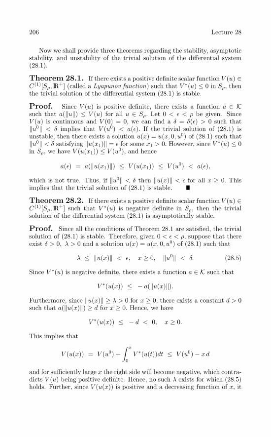
206 Lecture 28
Now we shall provide three theorems regarding the stability, asymptoticstability, and unstability of the trivial solution of the differential system(28.1).
Theorem 28.1. If there exists a positive definite scalar function V (u) ∈C(1)[Sρ, IR+] (called a Lyapunov function) such that V ∗(u) ≤ 0 in Sρ, thenthe trivial solution of the differential system (28.1) is stable.
Proof. Since V (u) is positive definite, there exists a function a ∈ Ksuch that a(‖u‖) ≤ V (u) for all u ∈ Sρ. Let 0 < ε < ρ be given. SinceV (u) is continuous and V (0) = 0, we can find a δ = δ(ε) > 0 such that‖u0‖ < δ implies that V (u0) < a(ε). If the trivial solution of (28.1) isunstable, then there exists a solution u(x) = u(x, 0, u0) of (28.1) such that‖u0‖ < δ satisfying ‖u(x1)‖ = ε for some x1 > 0. However, since V ∗(u) ≤ 0in Sρ, we have V (u(x1)) ≤ V (u0), and hence
a(ε) = a(‖u(x1)‖) ≤ V (u(x1)) ≤ V (u0) < a(ε),
which is not true. Thus, if ‖u0‖ < δ then ‖u(x)‖ < ε for all x ≥ 0. Thisimplies that the trivial solution of (28.1) is stable.
Theorem 28.2. If there exists a positive definite scalar function V (u) ∈C(1)[Sρ, IR+] such that V ∗(u) is negative definite in Sρ, then the trivialsolution of the differential system (28.1) is asymptotically stable.
Proof. Since all the conditions of Theorem 28.1 are satisfied, the trivialsolution of (28.1) is stable. Therefore, given 0 < ε < ρ, suppose that thereexist δ > 0, λ > 0 and a solution u(x) = u(x, 0, u0) of (28.1) such that
λ ≤ ‖u(x)‖ < ε, x ≥ 0, ‖u0‖ < δ. (28.5)
Since V ∗(u) is negative definite, there exists a function a ∈ K such that
V ∗(u(x)) ≤ − a(‖u(x)‖).
Furthermore, since ‖u(x)‖ ≥ λ > 0 for x ≥ 0, there exists a constant d > 0such that a(‖u(x)‖) ≥ d for x ≥ 0. Hence, we have
V ∗(u(x)) ≤ − d < 0, x ≥ 0.
This implies that
V (u(x)) = V (u0) +∫ x
0V ∗(u(t))dt ≤ V (u0) − x d
and for sufficiently large x the right side will become negative, which contra-dicts V (u) being positive definite. Hence, no such λ exists for which (28.5)holds. Further, since V (u(x)) is positive and a decreasing function of x, it
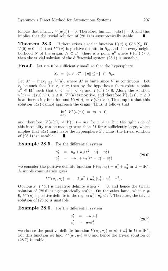
Lyapunov’s Direct Method for Autonomous Systems 207
follows that limx→∞ V (u(x)) = 0. Therefore, limx→∞ ‖u(x)‖ = 0, and thisimplies that the trivial solution of (28.1) is asymptotically stable.
Theorem 28.3. If there exists a scalar function V (u) ∈ C(1)[Sρ, IR],V (0) = 0 such that V ∗(u) is positive definite in Sρ, and if in every neigh-borhood N of the origin, N ⊂ Sρ, there is a point u0 where V (u0) > 0,then the trivial solution of the differential system (28.1) is unstable.
Proof. Let r > 0 be sufficiently small so that the hypersphere
Sr = u ∈ IRn : ‖u‖ ≤ r ⊂ Sρ.
Let M = max‖u‖≤r V (u), where M is finite since V is continuous. Letr1 be such that 0 < r1 < r; then by the hypotheses there exists a pointu0 ∈ IRn such that 0 < ‖u0‖ < r1 and V (u0) > 0. Along the solutionu(x) = u(x, 0, u0), x ≥ 0, V ∗(u) is positive, and therefore V (u(x)), x ≥ 0is an increasing function and V (u(0)) = V (u0) > 0. This implies that thissolution u(x) cannot approach the origin. Thus, it follows that
infx≥0
V ∗(u(x)) = m > 0,
and therefore, V (u(x)) ≥ V (u0) + mx for x ≥ 0. But the right side ofthis inequality can be made greater than M for x sufficiently large, whichimplies that u(x) must leave the hypersphere Sr. Thus, the trivial solutionof (28.1) is unstable.
Example 28.5. For the differential system
u′1 = u2 + u1(r2 − u2
1 − u22)
u′2 = −u1 + u2(r2 − u2
1 − u22)
(28.6)
we consider the positive definite function V (u1, u2) = u21 + u2
2 in Ω = IR2.A simple computation gives
V ∗(u1, u2) = − 2(u21 + u2
2)(u21 + u2
2 − r2).
Obviously, V ∗(u) is negative definite when r = 0, and hence the trivialsolution of (28.6) is asymptotically stable. On the other hand, when r =0, V ∗(u) is positive definite in the region u2
1+u22 < r2. Therefore, the trivial
solution of (28.6) is unstable.
Example 28.6. For the differential system
u′1 = −u1u
42
u′2 = u2u
41
(28.7)
we choose the positive definite function V (u1, u2) = u41 + u4
2 in Ω = IR2.For this function we find V ∗(u1, u2) ≡ 0 and hence the trivial solution of(28.7) is stable.

208 Lecture 28
Example 28.7. Consider the differential system (17.3) with aij(x) =−aji(x), i = j and aii(x) ≤ 0 for all x ≥ 0, and i, j = 1, 2, . . . , n. LetV (u) = u2
1 + · · · + u2n, which is obviously positive definite in Ω = IRn, and
V ∗(u) = 2n∑
i=1
ui(x)u′i(x) = 2
n∑i=1
ui(x)
⎡⎣ n∑
j=1
aij(x)uj(x)
⎤⎦
= 2n∑
i=1
n∑j=1
aij(x)ui(x)uj(x) = 2n∑
i=1
aii(x)u2i (x),
i.e., V ∗(u) is negative semidefinite. Therefore, the trivial solution of (17.3)is stable. If aii(x) < 0 for all x ≥ 0, then V ∗(u) is negative definite and thetrivial solution of (17.3) is asymptotically stable.
Example 28.8. Consider the Lienard equation (27.9), where the func-tions f(y) and g(y) are continuously differentiable for all y ∈ IR, g(0) = 0and yg(y) > 0 for all y = 0, and for some positive constant k, yF (y) > 0for y = 0, − k < y < k, where
F (y) =∫ y
0f(t)dt.
Equation (27.9) is equivalent to the system
u′1 = u2 − F (u1)
u′2 = −g(u1).
(28.8)
A suitable Lyapunov function for the differential system (28.8) is the totalenergy function V (u1, u2) = (1/2)u2
2 +G(u1), where
G(u1) =∫ u1
0g(t)dt.
Obviously, V (u1, u2) is positive definite in Ω = IR2. Further, it is easyto find V ∗(u) = −g(u1)F (u1). Thus, from our hypotheses it follows thatV ∗(u) ≤ 0 in the strip (u1, u2) ∈ IR2 : −k < u1 < k, − ∞ < u2 < ∞.Therefore, the trivial solution of (28.8) is stable.
Problems
28.1. Show that the function V (u1, u2) = c1u21 + c2u1u2 + c3u
22 in
Ω = IR2 is positive definite if and only if c1 > 0 and c22 − 4c1c3 < 0, and isnegative definite if and only if c1 < 0 and c22 − 4c1c3 < 0.

Lyapunov’s Direct Method for Autonomous Systems 209
28.2. For each of the following systems construct a Lyapunov functionof the form c1u
21 + c2u
22 to determine whether the trivial solution is stable,
asymptotically stable, or unstable:
(i)u′
1 = −u1 + eu1u2
u′2 = −eu1u1 − u2.
(ii)u′
1 = −u31 + u2
1u2
u′2 = −u3
1 − u21u2.
(iii)u′
1 = 2u2 − u1(1 + 4u22)
u′2 = (1/2)u1 − u2 + u2
1u2.(iv)
u′1 = 2u2 − 2u2 sinu1
u′2 = −u1 − 4u2 + u1 sinu1.
(v)u′
1 = −u1 + 2u21 + u2
2
u′2 = −u2 + u1u2.
(vi)u′
1 = −u1 − u2 − u31
u′2 = u1 − u2 − u3
2.
(vii)u′
1 = 2u1u2 + u31
u′2 = −u2
1 + u52.
(viii)u′
1 = u31 − u2
u′2 = u1 + u3
2.
28.3. Consider the system
u′1 = u2 − u1f(u1, u2)
u′2 = −u1 − u2f(u1, u2),
where f(u1, u2) has a convergent power series expansion in Ω ⊆ IR2 con-taining the origin, and f(0, 0) = 0. Show that the trivial solution of theabove system is
(i) stable if f(u1, u2) ≥ 0 in some region around the origin;(ii) asymptotically stable if f(u1, u2) is positive definite in some regionaround the origin;(iii) unstable if in every region around the origin there are points (u1, u2)such that f(u1, u2) < 0.
28.4. Use Problem 28.3 to determine whether the trivial solution isstable, asymptotically stable or unstable for each of the following systems:
(i)u′
1 = u2 − u1(eu1 sin2 u2)
u′2 = −u1 − u2(eu1 sin2 u2).
(ii)u′
1 = u2 − u1(u41 + u6
2 + 2u21u
22 sin2 u1)
u′2 = −u1 − u2(u4
1 + u62 + 2u2
1u22 sin2 u1).
(iii)u′
1 = u2 − u1(u32 sin2 u1)
u′2 = −u1 − u2(u3
2 sin2 u1).
28.5. Consider the equation of undamped simple pendulum y′′+ω2 sin y= 0, − π/2 ≤ y ≤ π/2. Prove by means of an appropriate Lyapunovfunction that its trivial solution is stable.
28.6. Prove by means of an appropriate Lyapunov function that the

210 Lecture 28
trivial solution of the Van der Pol equation (26.12) is asymptotically stablewhen µ < 0.
Answers or Hints
28.1. Completing the squares, we have
V (u1, u2) = c1
[(u1 + c2
2c1u2
)2+ 1
4c21
(4c1c3 − c22
)u2
2
].
28.2. (i) Asymptotically stable. (ii) Stable. (iii) Stable. (iv) Stable.(v) Asymptotically stable. (vi) Asymptotically stable. (vii) Unstable.(viii) Unstable.
28.3. Let V (u1, u2) = u21 + u2
2, then V ∗(u1, u2) = −2f(u1, u2)(u21 + u2
2).
28.4. (i) Stable. (ii) Asymptotically stable. (iii) Unstable.
28.5. Write the equation in system form and then use Lyapunov’s functionV (u1, u2) = g(u1) + 1
2u22, where g(u1) =
∫ u1
0 ω2 sin tdt.
28.6. Use V (u1, u2) = u21 + u2
2.

Lecture 29Lyapunov’s Direct Method
for Nonautonomous Systems
In this lecture we shall extend the method of Lyapunov functions tostudy the stability properties of the solutions of the differential system(15.1). For this, we shall assume that the function g(x, u) is continuous forall (x, u) ∈ [x0,∞)×Sρ, x0 ≥ 0 and smooth enough so that the initial valueproblem (15.4) has a unique solution in [x0,∞) for all u0 ∈ Sρ. Further, weshall assume that g(x, 0) ≡ 0 so that the differential system (15.1) admitsthe trivial solution. It is clear that a Lyapunov function for the system(15.1) must depend on x and u both, i.e., V = V (x, u).
Definition 29.1. A real-valued function V (x, u) defined in [x0,∞)×Sρ
is said to be positive definite if and only if V (x, 0) ≡ 0, x ≥ x0, and thereexists a function a(r) ∈ K such that a(r) ≤ V (x, u), ‖u‖ = r, (x, u) ∈[x0,∞) × Sρ. It is negative definite if V (x, u) ≤ −a(r).Definition 29.2. A real-valued function V (x, u) defined in [x0,∞)×Sρ
is said to be decrescent if and only if V (x, 0) ≡ 0, x ≥ x0 and there existsan h, 0 < h ≤ ρ and a function b(r) ∈ K such that V (x, u) ≤ b(‖u‖) for‖u‖ < h and x ≥ x0.
Example 29.1. The function
V (x, u1, u2) = (1 + sin2 x)u21 + (1 + cos2 x)u2
2
is positive definite in [0,∞) × IR2 since V (x, 0, 0) ≡ 0 and a(r) = r2 ∈ Ksatisfies the inequality a(r) ≤ V (x, u1, u2). This function is also decrescentsince b(r) = 2r2 ∈ K satisfies V (x, u1, u2) ≤ b(r).
Example 29.2. The function
V (x, u1, u2) = u21 + (1 + x2)u2
2
is positive definite in [0,∞) × IR2 but not decrescent since it can be arbi-trarily large for sufficiently small ‖u‖.Example 29.3. The function
V (x, u1, u2) = u21 +
1(1 + x2)
u22
R.P. Agarwal and D. O’Regan, An Introduction to Ordinary Differential Equations,
doi: 10.1007/978-0-387-71276-5_29, © Springer Science + Business Media, LLC 2008
211

212 Lecture 29
is decrescent. However, since
V (x, 0, u2) =1
(1 + x2)u2
2 → 0 as x → ∞,
we cannot find a suitable function a(r) ∈ K such that V (x, u1, u2) ≥ a(‖u‖),i.e., it is not positive definite.
Now we shall assume that V (x, u) ∈ C(1)[[x0,∞) × Sρ, IR] so that thechain rule can be used, to obtain
dV (x, u)dx
= V ∗(x, u) =∂V
∂x+
n∑i=1
∂V
∂ui
dui
dx.
Our interest is in the derivative of V (x, u) along a solution u(x) =u(x, x0, u
0) of the differential system (15.1). Indeed, we have
V ∗(x, u) =∂V
∂x+
n∑i=1
∂V
∂uigi(x, u) =
∂V
∂x+ gradV (x, u) · g(x, u).
The following two theorems regarding the stability and asymptotic sta-bility of the trivial solution of the differential system (15.1) are parallel tothe results in the autonomous case.
Theorem 29.1. If there exists a positive definite scalar functionV (x, u) ∈ C(1)[[x0,∞) × Sρ, IR+] (called a Lyapunov function) such thatV ∗(x, u) ≤ 0 in [x0,∞) × Sρ, then the trivial solution of the differentialsystem (15.1) is stable.
Theorem 29.2. If there exists a positive definite and decrescent scalarfunction V (x, u) ∈ C(1)[[x0,∞) × Sρ, IR+] such that V ∗(x, u) is negativedefinite in [x0,∞) × Sρ, then the trivial solution of the differential system(15.1) is asymptotically stable.
Example 29.4. Consider the DE y′′ + p(x)y = 0, where p(x) ≥ δ > 0and p′(x) ≤ 0 for all x ∈ [0,∞). This is equivalent to the system
u′1 = u2
u′2 = −p(x)u1.
(29.1)
For the differential system (29.1) we consider the scalar functionV (x, u1, u2) = p(x)u2
1+u22, which is positive definite in [0,∞)×IR2. Further,
since
V ∗(x, u) = p′(x)u21 + 2p(x)u1u2 + 2u2(−p(x)u1) = p′(x)u2
1 ≤ 0
in [0,∞) × IR2, the trivial solution of (29.1) is stable.

Lyapunov’s Direct Method for Nonautonomous Systems 213
Example 29.5. Consider the system
u′1 = −a11(x)u1 − a12(x)u2
u′2 = a21(x)u1 − a22(x)u2,
(29.2)
where a21(x) = a12(x), and a11(x) ≥ δ > 0, a22(x) ≥ δ > 0 for all x ∈[0,∞). For the differential system (29.2) we consider the scalar functionV (x, u1, u2) = u2
1 + u22 which is obviously positive definite and decrescent
in [0,∞) × IR2. Further, since
V ∗(x, u) = 2u1(−a11(x)u1 − a12(x)u2) + 2u2(a21(x)u1 − a22(x)u2)
= −2a11(x)u21 − 2a22(x)u2
2 ≤ − 2δ(u21 + u2
2)
in [0,∞) × IR2, the trivial solution of (29.2) is asymptotically stable.
We shall now formulate a result which provides sufficient conditions forthe trivial solution of the differential system (15.1) to be unstable.
Theorem 29.3. If there exists a scalar function V (x, u) ∈ C(1)[[x0,∞)×Sρ, IR] such that
(i) |V (x, u)| ≤ b(‖u‖) for all (x, u) ∈ [x0,∞) × Sρ, where b ∈ K;(ii) for every δ > 0 there exists an u0 with ‖u0‖ < δ such that V (x0, u
0) <0;(iii) V ∗(x, u) ≤ −a(‖u‖) for (x, u) ∈ [x0,∞) × Sρ, where a ∈ K,then the trivial solution of the differential system (15.1) is unstable.
Proof. Let the trivial solution of (15.1) be stable. Then for every ε > 0such that ε < ρ, there exists a δ = δ(ε) > 0 such that ‖u0‖ < δ implies that‖u(x)‖ = ‖u(x, x0, u
0)‖ < ε for all x ≥ x0. Let u0 be such that ‖u0‖ < δand V (x0, u
0) < 0. Since ‖u0‖ < δ, we have ‖u(x)‖ < ε. Hence, condition(i) gives
|V (x, u(x))| ≤ b(‖u(x)‖) < b(ε) for all x ≥ x0. (29.3)
Now from condition (iii), it follows that V (x, u(x)) is a decreasing function,and therefore for every x ≥ x0, we have V (x, u(x)) ≤ V (x0, u
0) < 0. Thisimplies that |V (x, u(x))| ≥ |V (x0, u
0)|. Hence, from condition (i) we get‖u(x)‖ ≥ b−1(|V (x0, u
0)|).From condition (iii) again, we have V ∗(x, u(x)) ≤ −a(‖u(x)‖), and
hence on integrating this inequality between x0 and x, we obtain
V (x, u(x)) ≤ V (x0, u0) −
∫ x
x0
a(‖u(t)‖)dt.

214 Lecture 29
However, since ‖u(x)‖ ≥ b−1(|V (x0, u0)|), it is clear that a(‖u(x)‖) ≥
a(b−1(|V (x0, u0)|)). Thus, we have
V (x, u(x)) ≤ V (x0, u0) − (x− x0)a(b−1(|V (x0, u
0)|)).
But this shows that limx→∞ V (x, u(x)) = −∞, which contradicts (29.3).Hence, the trivial solution of (15.1) is unstable.
Example 29.6. Consider the system
u′1 = a11(x)u1 − a12(x)u2
u′2 = a21(x)u1 + a22(x)u2,
(29.4)
where a21(x) = a12(x), and a11(x) ≥ δ > 0, a22(x) ≥ δ > 0 for all x ∈[0,∞). For the differential system (29.4) we consider the scalar functionV (x, u1, u2) = −(u2
1 + u22), and note that for all (x, u) ∈ [0,∞) × IR2,
|V (x, u1, u2)| ≤ (u21 +u2
2) = r2 = b(r) for (u1, u2) = (0, 0), V (x, u1, u2) < 0,and V ∗(x, u1, u2) = −2(a11(x)u2
1 + a22(x)u22) ≤ −2δ(u2
1 + u22) = −2δr2 =
−a(r). Thus, the conditions of Theorem 29.3 are satisfied and the trivialsolution of (29.4) is unstable.
Our final result in this lecture gives sufficient conditions for the trivialsolution of the differential system (15.1) to be uniformly stable.
Theorem 29.4. If there exists a positive definite and decrescentscalar function V (x, u) ∈ C(1)[[x0,∞) × Sρ, IR+] such that V ∗(x, u) ≤ 0in [x0,∞) × Sρ, then the trivial solution of the differential system (15.1) isuniformly stable.
Proof. Since V (x, u) is positive definite and decrescent, there existfunctions a, b ∈ K such that
a(‖u‖) ≤ V (x, u) ≤ b(‖u‖) (29.5)
for all (x, u) ∈ [x0,∞)×Sρ. For each ε, 0 < ε < ρ, we choose a δ = δ(ε) > 0such that b(δ) < a(ε). We now claim that the trivial solution of (15.1) isuniformly stable, i.e., if x1 ≥ x0 and ‖u(x1)‖ < δ, then ‖u(x)‖ < ε for allx ≥ x1. Suppose this is not true. Then there exists some x2 > x1 such thatx1 ≥ x0 and ‖u(x1)‖ < δ imply that
‖u(x2)‖ = ε. (29.6)
Integrating V ∗(x, u(x)) ≤ 0 from x1 to x, we get V (x, u(x)) ≤ V (x1, u(x1)),and hence for x = x2, we have
a(ε) = a(‖u(x2)‖) ≤ V (x2, u(x2)) ≤ V (x1, u(x1))
≤ b(‖u(x1)‖) ≤ b(δ) < a(ε).

Lyapunov’s Direct Method for Nonautonomous Systems 215
This contradicts relation (29.6), and therefore no such x2 exists. Hence,the trivial solution of (15.1) is uniformly stable.
Corollary 29.5. If there exists a scalar function V (x, u) ∈ C[[x0,∞)×Sρ, IR+] such that the inequality (29.5) holds, and V (x, u(x)) is nonincreas-ing in x for every solution u(x) of (15.1) with ‖u(x)‖ < ρ, then the trivialsolution of (15.1) is uniformly stable.
Example 29.7. For the differential system (29.2) once again we con-sider the scalar function V (x, u) = u2
1 + u22 and note that the inequality
(29.5) with a(r) = b(r) = r2 is satisfied. Further, since V ∗(x, u(x)) ≤ 0 forall solutions of (29.2), the trivial solution of (29.2) is uniformly stable.
To conclude, we remark that the main drawback of Lyapunov’s directmethod is that there is no sufficiently general constructive method for find-ing the function V (x, u). Nevertheless, for a series of important classes ofdifferential systems such a construction is possible.
Problems
29.1. Show the following:
(i) (u21 + u2
2) cos2 x is decrescent.(ii) u2
1 + exu22 is positive definite but not decrescent.
(iii) u21 + e−xu2
2 is decrescent.(iv) (1 + cos2 x+ e−2x)(u4
1 + u42) is positive definite and decrescent.
29.2. For the DE
y′ = (sin lnx+ cos lnx− 1.25)y, (29.7)
consider the function
V (x, y) = y2 exp(2(1.25 − sin lnx)x).
Show the following:
(i) V (x, y) is positive definite but not decrescent.(ii) The trivial solution of (29.7) is stable.
29.3. Show that the trivial solution of the differential system
u′1 = p(x)u2 + q(x)u1(u2
1 + u22)
u′2 = −p(x)u1 + q(x)u2(u2
1 + u22),
where p, q ∈ C[0,∞) is stable if q(x) ≤ 0, asymptotically stable if q(x) ≤δ < 0, and unstable if q(x) ≥ δ > 0.

216 Lecture 29
29.4. If there exists a positive definite scalar function V (x, u) ∈C(1)[[x0,∞) × Sρ, IR+] such that V ∗(x, u) ≤ −a(V (x, u)), where a ∈ K in[x0,∞) × Sρ, then show that the trivial solution of the differential system(15.1) is asymptotically stable.
29.5. For the DEy′ = (x sinx− 2x)y, (29.8)
consider the function
V (x, y) = y2 exp(∫ x
0(2t− t sin t)dt
).
Show the following:
(i) V (x, y) is positive definite but not decrescent.(ii) V ∗(x, y) ≤ −λV (x, y) for all x ≥ λ > 0.(iii) The trivial solution of (29.8) is asymptotically stable.
Answers or Hints
29.1. Verify directly.
29.2. Verify directly.
29.3. Use functions V (x, u1, u2) = u21 + u2
2 and V (x, u1, u2) = −(u21 + u2
2).
29.4. The stability of the trivial solution of (15.1) follows from Theorem29.1. Hence, given ε > 0 (0 < ε < ρ) there exists a δ = δ(ε) > 0 such that‖u0‖ < δ implies that ‖u(x, x0, u
0)‖ < ε for all x ≥ x0. Since V ∗(x, u) ≤−a(V (x, u)) along the trajectory through (x0, u
0), we have for all x ≥ x0∫ V (x,u)V (x0,u0)
dVa(V ) ≤ −(x− x0).
Thus, as x → ∞, the integral tends to −∞. But this is possible only ifV (x, u) → 0 as x → ∞. Now use the fact that V (x, u) is positive definite.
29.5. Verify directly.

Lecture 30Higher-Order Exact
and Adjoint Equations
The concept of exactness which was discussed for the first-order DEs inLecture 3 can be extended to higher-order DEs. The nth-order DE (1.5)is called exact if the function F (x, y, y′, . . . , y(n)) is a derivative of somedifferential expression of (n − 1)th order, say, φ(x, y, y′, . . . , y(n−1)). Thus,in particular, the second-order DE (6.1) is exact if
p0(x)y′′ + p1(x)y′ + p2(x)y = (p(x)y′ + q(x)y)′, (30.1)
where the functions p(x) and q(x) are differentiable in J.
Expanding (30.1), we obtain
p0(x)y′′ + p1(x)y′ + p2(x)y = p(x)y′′ + (p′(x) + q(x))y′ + q′(x)y,
and hence it is necessary that p0(x) = p(x), p1(x) = p′(x) + q(x), andp2(x) = q′(x) for all x ∈ J. These equations in turn imply that
p′′0(x) − p′
1(x) + p2(x) = 0. (30.2)
Thus, the DE (6.1) is exact if and only if condition (30.2) is satisfied.
Similarly, the second-order nonhomogeneous DE (6.6) is exact if theexpression p0(x)y′′ + p1(x)y′ + p2(x)y is exact, and in such a case (6.6) is
[p0(x)y′ + (p1(x) − p′0(x))y]
′ = r(x). (30.3)
On integrating (30.3), we find
p0(x)y′ + (p1(x) − p′0(x))y =
∫ x
r(t)dt+ c, (30.4)
which is a first-order linear DE and can be integrated to find the generalsolution of (6.6).
Example 30.1. For the DE
x2y′′ + xy′ − y = x4, x > 0
we have p′′0(x)− p′
1(x)+ p2(x) = 2− 1− 1 = 0, and hence it is an exact DE.Using (30.4), we get
x2y′ − xy =15x5 + c,
R.P. Agarwal and D. O’Regan, An Introduction to Ordinary Differential Equations,
doi: 10.1007/978-0-387-71276-5_30, © Springer Science + Business Media, LLC 2008
217

218 Lecture 30
which is a first-order linear DE. The general solution of this DE is
y(x) =115x4 +
c1x
+ c2x.
If the DE (6.1) is not exact, then we may seek an integrating factorz(x) that will make it exact. Such an integrating factor must satisfy thecondition
(p0(x)z(x))′′ − (p1(x)z(x))′ + p2(x)z(x) = 0. (30.5)
Equation (30.5) is a second-order DE in z(x) and it can be written as
q0(x)z′′ + q1(x)z′ + q2(x)z = 0, (30.6)
where
q0(x) = p0(x), q1(x) = 2p′0(x)−p1(x), q2(x) = p′′
0(x)−p′1(x)+p2(x).
(30.7)Equation (30.5), or equivalently (30.6), is in fact the adjoint equation of
(6.1). To show this, we note that the DE (6.1) is equivalent to the system[u′
1u′
2
]=
[0 1/p0(x)
−p2(x) (p′0(x) − p1(x))/p0(x)
] [u1u2
],
and its adjoint system is[v′1v′2
]=
[0 p2(x)
−1/p0(x) −(p′0(x) − p1(x))/p0(x)
] [v1v2
],
which is the same asv′1 = p2(x)v2 (30.8)
p0(x)v′2 = − v1 − (p′
0(x) − p1(x))v2. (30.9)
Now using (30.8) in (30.9), we obtain
p0(x)v′′2 + p′
0(x)v′2 = − p2(x)v2 − (p′′
0(x) − p′1(x))v2 − (p′
0(x) − p1(x))v′2,
or
p0(x)v′′2 + (2p′
0(x) − p1(x))v′2 + (p′′
0(x) − p′1(x) + p2(x))v2 = 0,
which is exactly the same as (30.6).
Obviously, relations (30.7) can be rewritten as
p0(x) = q0(x), p′0(x) − p1(x) = q1(x) − q′
0(x)
2p2(x) − p′1(x) = 2q2(x) − q′
1(x)(30.10)

Higher-Order Exact and Adjoint Equations 219
and hence when pi’s and qi’s are interchanged these equations are unaltered;thus the relation between equations (6.1) and (30.6) is of a reciprocal natureand each equation is the adjoint of the other.
When an equation and its adjoint are the same, it is said to be self-adjoint. Thus, the DE (6.1) is self-adjoint if p0(x) = q0(x), p1(x) =q1(x), p2(x) = q2(x). In such a situation, relations (30.7) give
p1(x) = p′0(x). (30.11)
Thus, the self-adjoint equation takes the form
p0(x)y′′ + p′0(x)y
′ + p2(x)y = 0,
which is the same as
(p0(x)y′)′ + p2(x)y = 0. (30.12)
Further, any self-adjoint equation can be written in the form (30.12).
The condition (30.11) shows that the DE (6.1) will become self-adjointafter multiplication by a function σ(x) that satisfies the relation
σ(x)p1(x) = (σ(x)p0(x))′,
which is the same as(σ(x)p0(x))′
σ(x)p0(x)=
p1(x)p0(x)
. (30.13)
On integrating (30.13), we easily find the function σ(x) which appears as
σ(x) =1
p0(x)exp
(∫ x p1(t)p0(t)
dt
). (30.14)
Thus, with this choice of σ(x) the DE
σ(x)p0(x)y′′ + σ(x)p1(x)y′ + σ(x)p2(x)y = 0 (30.15)
is a self-adjoint equation.
Since (30.15) is self-adjoint its solutions are also its integrating factors.But since (30.15) is the same as (6.1) multiplied by σ(x), the solutions of(6.1) are the solutions of (30.15). Hence the statement “the solutions of(30.15) are the integrating factors of (30.15)” is equivalent to saying that“σ(x) times the solutions of (6.1) are the integrating factors of (6.1).” But,since the integrating factors of (6.1) are the solutions of its adjoint equation(30.6), i.e., z(x) = σ(x)y(x) it follows that
z(x)y(x)
= σ(x) =1
p0(x)exp
(∫ x p1(t)p0(t)
dt
), (30.16)

220 Lecture 30
where y(x) and z(x) are solutions of (6.1) and (30.6), respectively.
Since (6.1) is adjoint of (30.6) it is also clear from (30.16) that
y(x)z(x)
=1
q0(x)exp
(∫ x q1(t)q0(t)
dt
). (30.17)
Example 30.2. The DE
xy′′ + 2y′ + a2xy = 0, x > 0
is not exact since p′′0 − p′
1 + p2 = a2x = 0. Its adjoint equation is
(xz)′′ − 2z′ + a2xz = x(z′′ + a2z) = 0,
whose general solution can be written as z(x) = c1 cos ax + c2 sin ax. Thefunction
σ(x) =1x
exp(∫ x 2
tdt
)= x.
Therefore, the general solution of the given DE is
y(x) =z(x)x
=c1 cos ax
x+c2 sin ax
x.
Now let the linear operator
P2 = p0(x)d2
dx2 + p1(x)d
dx+ p2(x)
and its adjoint
Q2 = q0(x)d2
dx2 + q1(x)d
dx+ q2(x),
so that the DEs (6.1) and (30.6), respectively, can be written as
P2[y] = p0(x)d2y
dx2 + p1(x)dy
dx+ p2(x)y = 0 (30.18)
and
Q2[z] = q0(x)d2z
dx2 + q1(x)dz
dx+ q2(x)z = 0. (30.19)

Higher-Order Exact and Adjoint Equations 221
Multiplying (30.18) by z and (30.19) by y and subtracting, we get
zP2[y] − yQ2[z]
= z(p0(x)y′′ + p1(x)y′ + p2(x)y) − y(q0(x)z′′ + q1(x)z′ + q2(x)z)
= z(p0(x)y′′ + p1(x)y′ + p2(x)y) − y((p0(x)z)′′ − (p1(x)z)′ + p2(x)z)
= (p0(x)z)y′′ − (p0(x)z)′′y + (p1(x)z)y′ + (p1(x)z)′y
=d
dx[(p0(x)z)y′ − (p0(x)z)′y] +
d
dx(p1(x)yz)
=d
dx[p0(x)(zy′ − z′y) + (p1(x) − p′
0(x))yz].
(30.20)Relation (30.20) is known as Lagrange’s identity. Further, the expressionin square brackets on the right side is called the bilinear concomitant of thefunctions y and z.
Integrating (30.20), we find
∫ β
α
(zP2[y] − yQ2[z])dx = [p0(x)(zy′ − z′y) + (p1(x) − p′0(x))yz]
∣∣∣∣∣β
α
.
(30.21)The relation (30.21) is called Green’s identity.
In the special case when the operator P2 is self-adjoint, i.e., p′0(x) =
p1(x), the Lagrange identity (30.20) reduces to
zP2[y] − yP2[z] =d
dx[p0(x)(zy′ − z′y)]. (30.22)
Thus, if y and z both are solutions of the DE (30.12), then (30.22) gives
p0(x)W (y, z)(x) = constant. (30.23)
Further, in this case Green’s identity (30.21) becomes
∫ β
α
(zP2[y] − yP2[z])dx = [p0(x)(zy′ − z′y)]
∣∣∣∣∣β
α
. (30.24)
Problems
30.1. Verify that the following DEs are exact and find their generalsolutions:
(i) y′′ + xy′ + y = 0.

222 Lecture 30
(ii) yy′′ + y′2 = 0.(iii) x2y′′ + (1 + 4x)y′ + 2y = 0, x > 0.(iv) (1 − x)y′′ + xy′ + y = 0, x = 1.
(v) (x+ 2xy)y′′ + 2xy′2 + 2y′ + 4yy′ = 0, x > 0.(vi) sinx y′′′ + cosx y′′ + sinx y′ + cosx y = 0, (0 < x < π).
30.2. If p1(x) = 2p′0(x), p2(x) = p′′
0(x), show that
p0(x)y′′ + p1(x)y′ + p2(x)y = (p0(x)y)′′
and hence find the general solution of the DE
(x2 + 3)y′′ + 4xy′ + 2y = e−x.
30.3. Show that the DE
p0(x)y(n) + p1(x)y(n−1) + · · · + pn(x)y = 0 (30.25)
is exact if and only if
p(n)0 (x) − p
(n−1)1 (x) + · · · + (−1)npn(x) = 0.
30.4. Show that the Euler equation (18.17) is exact if and only if
p0 − p1
n+
p2
n(n− 1)− · · · + (−1)n pn
n!= 0.
30.5. Transform the following equations to their self-adjoint forms:
(i) xy′′ − y′ + x3y = 0.(ii) x2y′′ + xy′ + (x2 − 1)y = 0.(iii) xy′′ + (1 − x)y′ + y = 0.
30.6. Solve the following equations with the help of their respectiveadjoint equations:
(i) xy′′ + (2x− 1)y′ + (x− 1)y = x2 + 2x− 2.(ii) x2y′′ + (3x2 + 4x)y′ + (2x2 + 6x+ 2)y = 0.
30.7. If z1(x) and z2(x) are linearly independent solutions of (30.6),show that y1(x) = z1(x)/σ(x) and y2(x) = z2(x)/σ(x) are linearly inde-pendent solutions of (6.1).
30.8. Show that the DE (6.19) has two solutions whose product is aconstant provided 2p1(x)p2(x) + p′
2(x) = 0. Hence, solve the DE
(x+ 1)x2y′′ + xy′ − (x+ 1)3y = 0.

Higher-Order Exact and Adjoint Equations 223
30.9. Show that a necessary and sufficient condition for transform-ing (6.19) into an equation with constant coefficients by a change of theindependent variable
φ = φ(x) =∫ x
[p2(t)]1/2dt
is that the function (p′2(x) + 2p1(x)p2(x))/p
3/22 (x) is a constant.
30.10. Show that if z(x) is an integrating factor of the DE (30.25); thenz(x) satisfies the adjoint DE
q0(x)z(n) − q1(x)z(n−1) + · · · + (−1)nqn(x)z = 0,
where
qk(x) =k∑
i=0
(−1)i
(n− k + i
i
)p(i)k−i(x)
= pk(x) −(n− k + 1
1
)p′
k−1(x) +(n− k + 2
2
)p′′
k−2(x) − · · · ,k = 0, 1, . . . , n.
Answers or Hints
30.1. (i) y′′ + xy′ + y = (y′ + xy)′, y = c1 exp(−x2/2) + c2 exp(−x2/2)×∫ x exp(t2/2)dt. (ii) yy′′ + (y′)2 = (yy′)′, y2 = c1x + c2. (iii) x2y′′ + (1 +4x)y′ +2y = (x2y′ +(1+2x)y)′, y = (c1/x2) exp(1/x)+ (c2/x2) exp(1/x)×∫ x exp(−1/t)dt. (iv) (1−x)y′′+xy′+y = ((1−x)y′+(1+x)y)′, y = c1e
x(1−x)2+c2ex(1−x)2 ∫ x[e−t/(1−t)3]dt. (v) (x+2xy)y′′+2x(y′)2+2y′+4yy′ =(xy(y+1))′′, xy(y+1) = c1x+c2. (vi) sinxy′′′+cosxy′′+sinxy′+cosxy =(sinxy′′ + sinxy)′, y = c1 cosx+ c2 sinx+ c3(−x cosx+ sinx ln sinx).
30.2. y = (c1 + c2x+ e−x)/(x2 + 3).
30.3.∑n
k=0 pk(x)y(n−k) = (∑n−1
k=0 qk(x)y(n−1−k))′ gives the relations p0 =q0, pk = qk + q′
k−1, k = 1, 2, . . . , n− 1, pn = q′n−1, which are equivalent to∑n
k=0(−1)kp(n−k)k (x) = 0.
30.4. Use Problem 30.3.
30.5. (i) σ(x) = 1/x2, (1/x)y′′−(1/x2)y′+xy = 0. (ii) σ(x) = 1/x, xy′′+y′ + [x− (1/x)]y = 0. (iii) σ(x) = e−x, xe−xy′′ + (1 − x)e−xy′ + e−xy = 0.
30.6. (i) e−x(c1 + c2x2) + 1 + x. (ii) e−x(c1 + c2e
−x)/x2.

224 Lecture 30
30.7. If z1(x), z2(x) are linearly independent solutions of (30.6), theny1(x) = z1(x)/σ(x), y2(x) = z2(x)/σ(x) are solutions of (6.1). DriveW (y1, y2)(x) = W (z1, z2)(x)/σ2(x).
30.8. Use y(x) = c/y1(x) in (6.19) to get the relation p2(x)y21 + y′2 = 0.
Differentiation of this relation and the fact that y1(x) is a solution givesp′2(x)y
21 − 2p1(x)y′
12 = 0, c1xex + c2e
−x/x.
30.9. Verify directly.
30.10. If z(x) is an integrating factor of (30.25), then it is necessary thatzp0y
(n) + zp1y(n−1) + · · · + zpny =
(q0y
(n−1) + q1y(n−2) + · · · + qn−1y
)′
= q0y(n) +(q1 + q′
0)y(n−1) +(q2 + q′
1)y(n−2) + · · ·+(qn−1 + q′
n−2)y′ + q′
n−1y,which implies that zp0 = q0, zpk = qk + q′
k−1, 1 ≤ k ≤ n− 1, zpn = qn−1and hence
(zp0)(n) − (zp1)(n−1) + (zp2)(n−2) − · · · + (−1)n(zpn) = 0.

Lecture 31Oscillatory Equations
In this lecture we shall consider the following second-order linear DE
(p(x)y′)′ + q(x)y = 0 (31.1)
and its special casey′′ + q(x)y = 0, (31.2)
where the functions p, q ∈ C(J), and p(x) > 0 for all x ∈ J. By a solutionof (31.1) we mean a nontrivial function y ∈ C(1)(J) and py′ ∈ C(1)(J). Asolution y(x) of (31.1) is said to be oscillatory if it has no last zero, i.e., ify(x1) = 0, then there exists an x2 > x1 such that y(x2) = 0. Equation (31.1)itself is said to be oscillatory if every solution of (31.1) is oscillatory. Asolution y(x) which is not oscillatory is called nonoscillatory. For example,the DE y′′ + y = 0 is oscillatory, whereas y′′ − y = 0 is nonoscillatory inJ = [0,∞).
From the practical point of view the following result is fundamental.
Theorem 31.1 (Sturm’s Comparison Theorem). If α, β ∈J are the consecutive zeros of a nontrivial solution y(x) of (31.2), and ifq1(x) is continuous and q1(x) ≥ q(x), q1(x) ≡ q(x) in [α, β], then everynontrivial solution z(x) of the DE
z′′ + q1(x)z = 0 (31.3)
has a zero in (α, β).
Proof. Multiplying (31.2) by z(x) and (31.3) by y(x) and subtracting,we obtain
z(x)y′′(x) − y(x)z′′(x) + (q(x) − q1(x))y(x)z(x) = 0,
which is the same as
(z(x)y′(x) − y(x)z′(x))′ + (q(x) − q1(x))y(x)z(x) = 0.
Since y(α) = y(β) = 0, an integration yields
z(β)y′(β) − z(α)y′(α) +∫ β
α
(q(x) − q1(x))y(x)z(x)dx = 0. (31.4)
R.P. Agarwal and D. O’Regan, An Introduction to Ordinary Differential Equations,
doi: 10.1007/978-0-387-71276-5_31, © Springer Science + Business Media, LLC 2008
225

226 Lecture 31
From the linearity of (31.2) we can assume that y(x) > 0 in (α, β), theny′(α) > 0 and y′(β) < 0. Thus, from (31.4) it follows that z(x) cannot beof fixed sign in (α, β), i.e., it has a zero in (α, β).
Corollary 31.2. If q(x) ≥ (1 + ε)/4x2, ε > 0 for all x > 0, then theDE (31.2) is oscillatory in J = (0,∞).
Proof. For ε > 0, all nontrivial solutions of the DE
y′′ +ε
4y = 0 (31.5)
are oscillatory. Let t = ex in (31.5), to obtain
t2d2y
dt2+ t
dy
dt+ε
4y = 0. (31.6)
Now using the substitution y = z/√t in (31.6), we find
d2z
dt2+
1 + ε
4t2z = 0. (31.7)
Since z(t) = ex/2y(ex) the equation (31.7) is also oscillatory. Therefore,from Theorem 31.1 between any two zeros of a solution of (31.7) thereis a zero of every solution of (31.2); i.e., DE (31.2) is oscillatory in J =(0,∞).
Example 31.1. Obviously the DE y′′ = 0 is nonoscillatory. Thus, ifthe function q(x) ≤ 0 (≡ 0) in J, Theorem 31.1 immediately implies thateach solution of the DE (31.2) cannot have more than one zero in J. Thus,in particular, the DE y′′ − x2y = 0 is nonoscillatory in J = IR.
Example 31.2. Obviously the DE y′′ + y = 0 is oscillatory. Thus, byTheorem 31.1 it follows that the DE y′′ + (1 + x)y = 0 is also oscillatory inJ = [0,∞).
Example 31.3. From Corollary 31.2 it is obvious that each solution ofthe DE y′′ +(c/x2)y = 0 has an infinite number of positive zeros if c > 1/4,and only a finite number of zeros if c < 1/4.
Example 31.4. Using the substitution y = u/√x it is easy to see that
the Bessel DEx2y′′ + xy′ + (x2 − a2)y = 0 (31.8)
can be transformed into a simple DE
u′′ +(
1 +1 − 4a2
4x2
)u = 0. (31.9)

Oscillatory Equations 227
We will use Theorem 31.1 to find the behavior of zeros of the solutions u(x)of the DE (31.9) in the interval J = (0,∞). For this, three cases are to bediscussed:
Case 1. If 0 ≤ a < 1/2, then 1 + [(1 − 4a2)/4x2] > 1 and hence fromTheorem 31.1 it follows that every solution u(x) of (31.9) must vanish atleast once between any two zeros of a nontrivial solution of z′′+z = 0. Sincefor a given p, sin(x− p) is a solution of z′′ + z = 0, we find that the zerosof this solution are p, p±π, p±2π, . . . . Thus, every solution u(x) of (31.9)has at least one zero in every subinterval of the positive x-axis of length π,i.e., the distance between successive zeros of u(x) does not exceed π.
Case 2. If a = 1/2, then the DE (31.9) reduces to u′′ + u = 0 and hencethe zeros of every solution u(x) of (31.9) are equally spaced by the distanceπ on the positive x-axis.
Case 3. If a > 1/2, then 1 + [(1 − 4a2)/4x2] < 1 and comparison withz′′ + z = 0 implies that every solution u(x) of (31.9) has at most one zeroin any subinterval of the positive x-axis of length π. To prove the existenceof zeros we reason as follows: For any fixed a, (1 − 4a2)/4x2 → 0 asx → ∞. Hence, there exists a x0 > 0 such that 1 + [(1 − 4a2)/4x2] > 1/2whenever x > x0, and now comparison with z′′ + (1/2)z = 0 implies thatevery solution u(x) of (31.9) has infinitely many zeros and that the distancebetween successive zeros eventually becomes less than
√2π.
We leave the proof of the fact that the distance between the successivezeros of every solution of (31.9) for every a tends to π (Problem 31.4).
Next we shall extend Sturm’s comparison theorem for the DE (31.1).For this, we need the following lemma.
Lemma 31.3 (Picone’s Identity). Let the functions y, z, py′,p1z
′ be differentiable and z(x) = 0 in J. Then the following identity holds:[yz(zpy′ − yp1z
′)]′
= y(py′)′ − y2
z(p1z
′)′ + (p− p1)y′2 + p1
(y′ − y
zz′)2.
(31.10)Proof. Expanding the left side, we have
y
z(z(py′)′ + z′py′ − y(p1z
′)′ − y′p1z′) +
(y′
z− y
z2 z′)
(zpy′ − yp1z′)
= y(py′)′ − y2
z(p1z
′)′ + py′2 − 2yy′p1z′
z+y2p1z
′2
z2
= y(py′)′ − y2
z(p1z
′)′ + (p− p1)y′2 + p1
(y′ − y
zz′)2.
Theorem 31.4 (Sturm–Picone’s Theorem). If α, β ∈ Jare the consecutive zeros of a nontrivial solution y(x) of (31.1), and if

228 Lecture 31
p1(x), q1(x) are continuous and 0 < p1(x) ≤ p(x), q1(x) ≥ q(x) in [α, β],then every nontrivial solution z(x) of the DE
(p1(x)z′)′ + q1(x)z = 0 (31.11)
has a zero in [α, β].
Proof. Let z(x) = 0 in [α, β], then Lemma 31.3 is applicable and from(31.10) and the DEs (31.1) and (31.11), we find[y
z(zpy′ − yp1z
′)]′
= (q1 − q)y2 + (p− p1)y′2 + p1
(y′ − y
zz′)2.
Integrating the above identity and using y(α) = y(β) = 0, we obtain∫ β
α
[(q1 − q)y2 + (p− p1)y′2 + p1
(y′ − y
zz′)2]dx = 0,
which is a contradiction unless q1(x) ≡ q(x), p1(x) ≡ p(x) and y′ −(y/z)z′ ≡ 0. The last identity is the same as d(y/z)/dx ≡ 0, and hencey(x)/z(x) ≡ constant. However, since y(α) = 0 this constant must be zero,and so y(x)/z(x) ≡ 0, or y(x) ≡ 0. This contradiction implies that z musthave a zero in [α, β].
Corollary 31.5 (Sturm’s Separation Theorem). If y1(x)and y2(x) are two linearly independent solutions of the DE (31.1) in J, thentheir zeros are interlaced, i.e., between two consecutive zeros of one thereis exactly one zero of the other.
Proof. Since y1(x) and y2(x) cannot have common zeros, Theorem 31.4(p1(x) ≡ p(x), q1(x) ≡ q(x)) implies that the solution y2(x) has at leastone zero between two consecutive zeros of y1(x). Interchanging y1(x) andy2(x) we see that y2(x) has at most one zero between two consecutive zerosof y1(x).
Example 31.5. It is easy to see that the functions y1(x) = c1 cosx+c2 sinx and y2(x) = c3 cosx+ c4 sinx are linearly independent solutions ofthe DE y′′ + y = 0 if and only if c1c4 − c2c3 = 0. Thus, from Corollary 31.5it follows that these functions y1(x) and y2(x) have alternating zeros.
In a finite interval J = [α, β] the DE (31.1) can have at most finitenumber of zeros, and this we shall prove in the following result.
Theorem 31.6. The only solution of the DE (31.1) which vanishesinfinitely often in J = [α, β] is the trivial solution.
Proof. We assume that the solution y(x) of the DE (31.1) has aninfinite number of zeros in J. The set of zeros will then have a limit pointx∗ ∈ J, and there will exist a sequence xm of zeros converging to x∗ with

Oscillatory Equations 229
xm = x∗, m = 0, 1, . . . . We shall show that y(x∗) = y′(x∗) = 0, then fromthe uniqueness of solutions it will follow that y(x) ≡ 0 in J. For this, thecontinuity of the solution y(x) implies that y(x∗) = limm→∞ y(xm) = 0.Next from the differentiability of the solution y(x), we have
y′(x∗) = limm→∞
y(xm) − y(x∗)xm − x∗ = 0.
The final result in this lecture gives an easier test for the DE (31.1) tobe oscillatory in J = (0,∞).
Theorem 31.7 (Leighton’s Oscillation Theorem). If∫∞(1/p(x))dx = ∞ and∫∞
q(x)dx = ∞, then the DE (31.1) is oscilla-tory in J = (0,∞).
Proof. Let y(x) be a nonoscillatory solution of the DE (31.1) which weassume to be positive in [x0,∞), where x0 > 0. Then from Problem 31.7the Riccati equation
z′ + q(x) +z2
p(x)= 0 (31.12)
has a solution z(x) in [x0,∞). This solution obviously satisfies the equation
z(x) = z(x0) −∫ x
x0
q(t)dt−∫ x
x0
z2(t)p(t)
dt. (31.13)
Since∫∞
q(t)dt = ∞, we can always find an x1 > x0 such that
z(x0) −∫ x
x0
q(t)dt < 0
for all x in [x1,∞). Thus, from (31.13) it follows that
z(x) < −∫ x
x0
z2(t)p(t)
dt
for all x ∈ [x1,∞). Let
r(x) =∫ x
x0
z2(t)p(t)
dt, x ∈ [x1,∞)
then z(x) < −r(x) and
r′(x) =z2(x)p(x)
>r2(x)p(x)
(31.14)
for all x in [x1,∞). Integrating (31.14) from x1 > x0 to ∞, we obtain
− 1r(∞)
+1
r(x1)>
∫ ∞
x1
1p(t)
dt

230 Lecture 31
and hence ∫ ∞
x1
1p(t)
dt <1
r(x1)< ∞,
which is a contradiction. Thus, the solution y(x) is oscillatory.
Example 31.6. Once again we consider the DE (31.9). For all a,there exists a sufficiently large x0 such that 1 + [(1 − 4a2)/4x2] > 1/2 forall x ≥ x0, and hence ∫ ∞(
1 +1 − 4a2
4x2
)dx = ∞.
Thus, Theorem 31.7 implies that (31.9) is oscillatory for all a.
Problems
31.1. Let the function q1(x) be continuous and q1(x) ≥ q(x) in J. Showthe following:
(i) If DE (31.2) is oscillatory, then the DE (31.3) is oscillatory.(ii) If DE (31.3) is nonoscillatory, then the DE (31.2) is nonoscillatory.
31.2. Show that the DE (31.2) is oscillatory if any one of the followingconditions is satisfied:(i) q(x) ≥ m2 > 0 eventually.(ii) q(x) = 1 + φ(x), where φ(x) → 0 as x → ∞.(iii) q(x) → ∞ as x → ∞.
31.3. Let the function q(x) be such that 0 < m ≤ q(x) ≤ M in [α, β].Further, let α ≤ x1 < x2 < · · · < xn ≤ β be the zeros of a solution y(x) ofthe DE (31.2). Then show the following:
(i) π/√m ≥ xi+1 − xi ≥ π/
√M, i = 1, 2, . . . , n− 1.
(ii) n > (β − α)(√m/π) − 1.
31.4. Use Problem 31.3 to show that the distance between the succes-sive zeros of every solution of (31.9) for each a tends to π.
31.5. Let the function q1(x) be continuous and q1(x) ≥ q(x), q1(x) ≡q(x) in [α, β]. Further, let y(x) and z(x) be respective solutions of (31.2)and (31.3) such that y′(α)/y(α) ≥ z′(α)/z(α), y(α) = 0, z(α) = 0, ory(α) = z(α) = 0.
(i) Use Sturm’s comparison theorem to show that z(x) has at least asmany zeros in [α, β] as y(x).

Oscillatory Equations 231
(ii) Further, if y(x) and z(x) have the same number of zeros, then showthat y′(β)/y(β) > z′(β)/z(β) provided y(β) = 0.
31.6. Give an example to show that Sturm’s separation theorem neednot be true for DEs of order higher than two.
31.7. Show that the DE (31.1) has a solution without zeros in aninterval J if and only if the Riccati equation (31.12) has a solution definedthroughout J.
31.8. Show that every solution of the Hermite DE y′′ − 2xy′ + 2ay =0 (a ≥ 0) has at most finitely many zeros in the interval J = IR.
31.9. Let p, q ∈ C(1)(J), q(x) = 0 in J and p(x)q(x) be nonincreasing(nondecreasing) in J. Then show that the absolute values of the relativemaxima and minima of every solution y(x) of the DE (31.1) are nonde-creasing (nonincreasing) as x increases.
31.10. Use Problem 31.9 to show that the magnitude of the oscillationsof each solution of the Bessel equation (31.8) is nonincreasing in the interval(a,∞).
Answers or Hints
31.1. (i) Use Theorem 31.1. (ii) Use part (i).
31.2. Use Problem 31.1.
31.3. (i) Compare (31.2) with y′′ +my = 0 and y′′ +My = 0 and applyTheorem 31.1. (ii) Note that each of the intervals [α, x1] and [xn, β] is oflength less than π/
√m.
31.4. Note that 1 − ε ≤ q(x) = 1 + 1−4a2
4x2 ≤ 1 + ε for all sufficiently largex, say, x ≥ x∗. Thus, in view of Problem 31.3(i), if xi, xi+1(≥ x∗) are twoconsecutive zeros of the solution u(x) of (31.9), then
π√(1+ε)
≤ xi+1 − xi ≤ π√(1−ε)
.
31.5. (i) If the zeros of y(x) are (α ≤)x1 < x2 < · · · < xn(≤ β), then byTheorem 31.1, z(x) has at least (n − 1) zeros in (x1, xn). Thus, it sufficesto show that z(x) has a zero in [α, x1]. If y(α) = z(α) = 0, then the proofis complete, otherwise, as in Theorem 31.1 we have
(z(x)y′(x) − y(x)z′(x))|x1α =
∫ x1
α(q1(x) − q(x))y(x)z(x)dx.
Thus, if y(x) > 0, x ∈ [α, x1) and z(x) > 0, x ∈ [α, x1], then z(x1)y′(x1) −(z(α)y′(α) − y(α)z′(α)) > 0. But, now y′(x1) < 0 and y′(α)
y(α) ≥ z′(α)z(α) leads
to a contradiction. (ii) Use part (i).

232 Lecture 31
31.6. Consider y′′′ + y = 0.
31.7. Use py′ = zy.
31.8. Use z(x) = e−x2/2y(x) to obtain z′′ + (1 + 2a− x2)z = 0.
31.9. For a nontrivial solution y(x) of (31.1) consider the function g =
y2 + 1pq (py′)2; then g′ = −
(y′
q
)2(pq)′. Now if (pq)′ ≤ 0 then g′ ≥ 0.
31.10. The self-adjoint form of (31.8) is (xy′)′ +(
x2−a2
x
)y = 0. Clearly,
p(x)q(x) = x2 − a2 is increasing and positive in (a,∞).

Lecture 32Linear BoundaryValue Problems
So far, we have concentrated only on initial value problems, in whichfor a given DE the supplementary conditions on the unknown function andits derivatives are prescribed at a fixed value x0 of the independent variablex. However, as we have indicated in Lecture 1 there are a variety of otherpossible conditions that are important in applications. In many practicalproblems the additional requirements are given in the form of boundaryconditions: the unknown function and some of its derivatives are fixed atmore than one value of the independent variable x. The DE together withthe boundary conditions are referred to as a boundary value problem.
Consider the second-order linear DE (6.6) in the interval J = [α, β],where, as we did earlier, we assume that the functions p0(x), p1(x), p2(x)and r(x) are continuous in J. Together with the DE (6.6) we shall considerthe boundary conditions of the form
1[y] = a0y(α) + a1y′(α) + b0y(β) + b1y
′(β) = A
2[y] = c0y(α) + c1y′(α) + d0y(β) + d1y
′(β) = B,(32.1)
where ai, bi, ci, di, i = 0, 1 and A, B are given constants. Throughout,we shall assume that these are essentially two conditions, i.e., there doesnot exist a constant c such that (a0 a1 b0 b1) = c(c0 c1 d0 d1). Boundaryvalue problem (6.6), (32.1) is called a nonhomogeneous two point linearboundary value problem, whereas the homogeneous DE (6.1) together withthe homogeneous boundary conditions
1[y] = 0, 2[y] = 0 (32.2)
will be called a homogeneous boundary value problem.
Boundary conditions (32.1) are quite general and, in particular, in-clude the
(i) first boundary conditions (Dirichlet conditions)
y(α) = A, y(β) = B, (32.3)
(ii) second boundary conditions (mixed conditions)
y(α) = A, y′(β) = B, (32.4)
R.P. Agarwal and D. O’Regan, An Introduction to Ordinary Differential Equations,
doi: 10.1007/978-0-387-71276-5_32, © Springer Science + Business Media, LLC 2008
233

234 Lecture 32
ory′(α) = A, y(β) = B, (32.5)
(iii) separated boundary conditions (third boundary conditions)
a0y(α) + a1y′(α) = A
d0y(β) + d1y′(β) = B,
(32.6)
where both a20 + a2
1 and d20 + d2
1 are different from zero, and(iv) periodic boundary conditions
y(α) = y(β), y′(α) = y′(β). (32.7)
Boundary value problem (6.6), (32.1) is called regular if both α and βare finite, and the function p0(x) = 0 for all x ∈ J. If α = −∞ and/orβ = ∞ and/or p0(x) = 0 for at least one point x in J, then the problem(6.6), (32.1) is said to be singular. We shall consider only regular boundaryvalue problems.
By a solution of the boundary value problem (6.6), (32.1) we mean asolution of the DE (6.6) satisfying the boundary conditions (32.1).
The existence and uniqueness theory for the boundary value problemsis more difficult than that of initial value problems. In fact, in the case ofboundary value problems a slight change in the boundary conditions canlead to significant changes in the behavior of the solutions. For example, theinitial value problem y′′+y = 0, y(0) = c1, y
′(0) = c2 has a unique solutiony(x) = c1 cosx+c2 sinx for any set of values c1, c2. However, the boundaryvalue problem y′′ + y = 0, y(0) = 0, y(π) = ε(= 0) has no solution; theproblem y′′ + y = 0, y(0) = 0, y(β) = ε, 0 < β < π has a unique solutiony(x) = ε sinx/ sinβ, while the problem y′′ + y = 0, y(0) = 0, y(π) = 0has an infinite number of solutions y(x) = c sinx, where c is an arbitraryconstant. Similarly, since for the DE (1+x2)y′′ −2xy′ +2y = 0 the generalsolution is y(x) = c1(x2 − 1)+ c2x, there exists a unique solution satisfyingthe boundary conditions y′(α) = A, y′(β) = B; an infinite number ofsolutions satisfying y(−1) = 0 = y(1); and no solution satisfying y(−1) =0, y(1) = 1.
Obviously, for the homogeneous problem (6.1), (32.2) the trivial so-lution always exists. However, from the above examples it follows thatbesides having the trivial solution, homogeneous boundary value problemsmay have nontrivial solutions also. Our first result provides necessary andsufficient condition so that the problem (6.1), (32.2) has only the trivialsolution.
Theorem 32.1. Let y1(x) and y2(x) be any two linearly independentsolutions of the DE (6.1). Then the homogeneous boundary value problem

Linear Boundary Value Problems 235
(6.1), (32.2) has only the trivial solution if and only if
∆ =
∣∣∣∣∣ 1[y1] 1[y2]
2[y1] 2[y2]
∣∣∣∣∣ = 0. (32.8)
Proof. Any solution of the DE (6.1) can be written as
y(x) = c1y1(x) + c2y2(x).
This is a solution of the problem (6.1), (32.2) if and only if
1[c1y1 + c2y2] = c11[y1] + c21[y2] = 0
2[c1y1 + c2y2] = c12[y1] + c22[y2] = 0.(32.9)
However, from Theorem 13.2, system (32.9) has only the trivial solution ifand only if ∆ = 0.
Clearly, Theorem 32.1 is independent of the choice of the solutions y1(x)and y2(x). Thus, for convenience we can always take y1(x) and y2(x) to bethe solutions of (6.1) satisfying the initial conditions
y1(α) = 1, y′1(α) = 0 (32.10)
andy2(α) = 0, y′
2(α) = 1. (32.11)
Corollary 32.2. The homogeneous boundary value problem (6.1),(32.2) has an infinite number of nontrivial solutions if and only if ∆ = 0.
Example 32.1. Consider the boundary value problem
xy′′ − y′ − 4x3y = 0 (32.12)
1[y] = y(1) = 0
2[y] = y(2) = 0.(32.13)
For the DE (32.12), y1(x) = cosh(x2 − 1) and y2(x) = (1/2) sinh(x2 − 1)are two linearly independent solutions. Further, since for the boundaryconditions (32.13), we have
∆ =
∣∣∣∣∣ 1 0
cosh 3 (1/2) sinh 3
∣∣∣∣∣ = 0
the problem (32.12), (32.13) has only the trivial solution.
Example 32.2. Consider once again the DE (32.12) together with theboundary conditions
1[y] = y′(1) = 0
2[y] = y′(2) = 0.(32.14)

236 Lecture 32
Since y′1(x) = 2x sinh(x2 − 1) and y′
2(x) = x cosh(x2 − 1), for the boundaryconditions (32.14), we find
∆ =
∣∣∣∣∣ 0 1
4 sinh 3 2 cosh 3
∣∣∣∣∣ = 0.
Thus, the problem (32.12), (32.14) has only the trivial solution.
Example 32.3. Consider the boundary value problem
y′′ + 2y′ + 5y = 0 (32.15)
1[y] = y(0) = 0
2[y] = y(π/2) = 0.(32.16)
For the DE (32.15), y1(x) = e−x cos 2x and y2(x) = e−x sin 2x are twolinearly independent solutions. Further, since for the boundary conditions(32.16),
∆ =
∣∣∣∣∣ 1 0
−e−π/2 0
∣∣∣∣∣ = 0
the problem (32.15), (32.16) besides having the trivial solution also hasnontrivial solutions. Indeed it has an infinite number of solutions y(x) =ce−x sin 2x, where c is an arbitrary constant.
Theorem 32.3. The nonhomogeneous boundary value problem (6.6),(32.1) has a unique solution if and only if the homogeneous boundary valueproblem (6.1), (32.2) has only the trivial solution.
Proof. Let y1(x) and y2(x) be any two linearly independent solutions ofthe DE (6.1) and z(x) be a particular solution of (6.6). Then the generalsolution of (6.6) can be written as
y(x) = c1y1(x) + c2y2(x) + z(x). (32.17)
This is a solution of the problem (6.6), (32.1) if and only if
1[c1y1 + c2y2 + z] = c11[y1] + c21[y2] + 1[z] = A
2[c1y1 + c2y2 + z] = c12[y1] + c22[y2] + 2[z] = B.(32.18)
However, from Theorem 13.2, nonhomogeneous system (32.18) has a uniquesolution if and only if ∆ = 0, i.e., if and only if the homogeneous system(32.9) has only the trivial solution. From Theorem 32.1, ∆ = 0 is equivalentto the homogeneous boundary value problem (6.1), (32.2) having only thetrivial solution.
Example 32.4. Consider the boundary value problem
xy′′ − y′ − 4x3y = 1 + 4x4 (32.19)

Linear Boundary Value Problems 237
1[y] = y(1) = 0
2[y] = y(2) = 1.(32.20)
Since the corresponding homogeneous problem (32.12), (32.13) has only thetrivial solution, Theorem 32.3 implies that the problem (32.19), (32.20) hasa unique solution. Further, to find this solution once again we choose thelinearly independent solutions of (32.12) to be y1(x) = cosh(x2 − 1) andy2(x) = (1/2) sinh(x2 −1), and note that z(x) = −x is a particular solutionof (32.19). Thus, the system (32.18) for the boundary conditions (32.20)reduces to
c1 − 1 = 0
cosh 3 c1 + (1/2) sinh 3 c2 − 2 = 1.
This system can be solved easily, and we obtain c1 = 1 and c2 =2(3 − cosh 3)/ sinh 3. Now substituting these quantities in (32.17) we findthe solution of (32.19), (32.20) as
y(x) = cosh(x2 − 1) +(3 − cosh 3)
sinh 3sinh(x2 − 1) − x.
Problems
32.1. Solve the following boundary value problems:
(i)y′′ − y = 0y(0) = 0, y(1) = 1. (ii)
y′′ + 4y′ + 7y = 0y(0) = 0, y′(1) = 1.
(iii)y′′ − 6y′ + 25y = 0y′(0) = 1, y(π/4) = 0. (iv)
x2y′′ + 7xy′ + 3y = 0y(1) = 1, y(2) = 2.
(v)y′′ + y = 0y(0) + y′(0) = 10y(1) + 3y′(1) = 4.
(vi)y′′ + y = x2
y(0) = 0, y(π/2) = 1.
(vii)y′′ + 2y′ + y = xy(0) = 0, y(2) = 3. (viii)
y′′ + y′ + y = xy(0) + 2y′(0) = 1y(1) − y′(1) = 8.
32.2. Show that the following boundary value problem has no solution:
y′′ + y = x, y(0) + y′(0) = 0, y(π/2) − y′(π/2) = π/2.
32.3. Solve the following periodic boundary value problems:
(i)y′′ + 2y′ + 10y = 0y(0) = y(π/6)y′(0) = y′(π/6).
(ii)y′′ + π2y = 0y(−1) = y(1)y′(−1) = y′(1).

238 Lecture 32
32.4. Show that the boundary value problem y′′ = r(x), (32.6) has aunique solution if and only if
∆ = a0d0(β − α) + a0d1 − a1d0 = 0.
32.5. Determine the values of the constants β, A, and B so that theboundary value problem y′′ + 2py′ + qy = 0, y(0) = A, y(β) = B withp2 − q < 0 has only one solution.
32.6. Show that the boundary value problem y′′ +p(x)y = q(x), (32.3)where p(x) ≤ 0 in [α, β] has a unique solution.
32.7. Let z(x) be the solution of the initial value problem (6.6), z(α) =A, z′(α) = 0 and y2(x) be the solution of the initial value problem (6.1),(32.11). Show that the boundary value problem (6.6), (32.3) has a uniquesolution y(x) if and only if y2(β) = 0 and it can be written as
y(x) = z(x) +(B − z(β))y2(β)
y2(x).
32.8. Let y1(x) and y2(x) be the solutions of the initial value problems(6.1), y1(α) = a1, y
′1(α) = −a0 and (6.1), y2(β) = −d1, y
′2(β) = d0,
respectively. Show that the boundary value problem (6.6), (32.6) has aunique solution if and only if W (y1, y2)(α) = 0.
32.9. Let y1(x) and y2(x) be the solutions of the boundary valueproblems (6.1), (32.1) and (6.6), (32.2), respectively. Show that y(x) =y1(x) + y2(x) is a solution of the problem (6.6), (32.1).
32.10. For the homogeneous DE
L2[y] = (x2 + 1)y′′ − 2xy′ + 2y = 0 (32.21)
x and (x2 −1) are two linearly independent solutions. Use this informationto show that the boundary value problem
L2[y] = 6(x2 + 1)2, y(0) = 1, y(1) = 2 (32.22)
has a unique solution, and find it.
Answers or Hints
32.1. (i) sinh xsinh 1 . (ii) e2(1−x) sin
√3x
(√
3 cos√
3−2 sin√
3). (iii) 1
4e3x sin 4x. (iv) 1
(2√
6−2−√6)
×[(16−2−√
6)x−3+√
6+(2√
6−16)x−3−√6]. (v) 1
2 sin 1+cos 1 [5(sin 1+3 cos 1)−2 cosx+5(3 sin 1−cos 1)+2 sinx]. (vi) 2 cosx+
(3 − π2
4
)sinx+x2 −2.

Linear Boundary Value Problems 239
(vii) e−x[2 +
( 32e
2 − 1)x]+ x− 2. (viii) 18
3 cos√
32 +
√3 sin
√3
2
e(1−x)/2 cos√
32 x
+x− 1.
32.2. Leads to an inconsistent system of equations.
32.3. (i) Trivial solution. (ii) c1 cosπx + c2 sinπx, where c1 and c2 arearbitrary constants.
32.4. For the DE y′′ = 0 two linearly independent solutions are 1, x. Nowapply Theorem 32.3.
32.5. β = nπ√q−p2
, e−px
[A cos
√q−p2x+ Bepβ−A cos
√q−p2β
sin√
q−p2βsin
√q − p2x
].
32.6. Use Theorem 32.3 and Example 31.1.
32.7. The function y(x) = z1(x) + cy1(x) is a solution of the DE (6.6).
32.8. Use Theorem 32.3.
32.9. Verify directly.
32.10. Use variation of parameters to find the particular solution z(x) =x4 + 3x2. The solution of (32.22) is x4 + 2x2 − 2x+ 1.

Lecture 33Green’s Functions
The function H(x, t) defined in (6.10) is a solution of the homogeneousDE (6.1) and it helps in finding an explicit representation of a particularsolution of the nonhomogeneous DE (6.6) (also see Problem 18.9 for higher-order DEs). In this lecture, we shall find an analog of this function calledGreen’s functionG(x, t) for the homogeneous boundary value problem (6.1),(32.2) and show that the solution of the nonhomogeneous boundary valueproblem (6.6), (32.2) can be explicitly expressed in terms of G(x, t). Thesolution of the problem (6.6), (32.1) then can be obtained easily as anapplication of Problem 32.9. For this, in what follows throughout we shallassume that the problem (6.1), (32.2) has only the trivial solution. Green’sfunction G(x, t) for the boundary value problem (6.1), (32.2) is defined inthe square [α, β]×[α, β] and possesses the following fundamental properties:
(i) G(x, t) is continuous in [α, β] × [α, β].
(ii) ∂G(x, t)/∂x is continuous in each of the triangles α ≤ x ≤ t ≤ β andα ≤ t ≤ x ≤ β; moreover
∂G
∂x(t+, t) − ∂G
∂x(t−, t) =
1p0(t)
,
where
∂G
∂x(t+, t) = lim
x → tx > t
∂G(x, t)∂x
and∂G
∂x(t−, t) = lim
x → tx < t
∂G(x, t)∂x
.
(iii) For every t ∈ [α, β], z(x) = G(x, t) is a solution of the DE (6.1) ineach of the intervals [α, t) and (t, β].
(iv) For every t ∈ [α, β], z(x) = G(x, t) satisfies the boundary conditions(32.2).
These properties completely characterize Green’s function G(x, t). Toshow this, let y1(x) and y2(x) be two linearly independent solutions ofthe DE (6.1). From the property (iii) there exist four functions, say,λ1(t), λ2(t), µ1(t), and µ2(t) such that
G(x, t) =
y1(x)λ1(t) + y2(x)λ2(t), α ≤ x ≤ t
y1(x)µ1(t) + y2(x)µ2(t), t ≤ x ≤ β.(33.1)
R.P. Agarwal and D. O’Regan, An Introduction to Ordinary Differential Equations,
doi: 10.1007/978-0-387-71276-5_33, © Springer Science + Business Media, LLC 2008
240

Green’s Functions 241
Now using properties (i) and (ii), we obtain the following two equations:
y1(t)λ1(t) + y2(t)λ2(t) = y1(t)µ1(t) + y2(t)µ2(t) (33.2)
y′1(t)µ1(t) + y′
2(t)µ2(t) − y′1(t)λ1(t) − y′
2(t)λ2(t) =1
p0(t). (33.3)
Let ν1(t) = µ1(t)−λ1(t) and ν2(t) = µ2(t)−λ2(t), so that (33.2) and (33.3)can be written as
y1(t)ν1(t) + y2(t)ν2(t) = 0 (33.4)
y′1(t)ν1(t) + y′
2(t)ν2(t) =1
p0(t). (33.5)
Since y1(x) and y2(x) are linearly independent the WronskianW (y1, y2)(t)= 0 for all t ∈ [α, β]. Thus, the relations (33.4), (33.5) uniquely determineν1(t) and ν2(t).
Now using the relations µ1(t) = λ1(t) + ν1(t) and µ2(t) = λ2(t) + ν2(t),Green’s function can be written as
G(x, t) =
y1(x)λ1(t) + y2(x)λ2(t), α ≤ x ≤ t
y1(x)λ1(t) + y2(x)λ2(t) + y1(x)ν1(t) + y2(x)ν2(t), t ≤ x ≤ β.
(33.6)Finally, using the property (iv), we find
1[y1]λ1(t) + 1[y2]λ2(t) = −b0(y1(β)ν1(t) + y2(β)ν2(t))−b1(y′
1(β)ν1(t) + y′2(β)ν2(t))
2[y1]λ1(t) + 2[y2]λ2(t) = −d0(y1(β)ν1(t) + y2(β)ν2(t))−d1(y′
1(β)ν1(t) + y′2(β)ν2(t)).
(33.7)
Since the problem (6.1), (32.2) has only the trivial solution, from Theorem32.1 it follows that the system (33.7) uniquely determines λ1(t) and λ2(t).
From the above construction it is clear that no other function existswhich has properties (i)–(iv), i.e., Green’s function G(x, t) of the boundaryvalue problem (6.1), (32.2) is unique.
As claimed earlier, we shall now show that the unique solution y(x) ofthe problem (6.6), (32.2) can be represented in terms of G(x, t) as follows:
y(x) =∫ β
α
G(x, t)r(t)dt =∫ x
α
G(x, t)r(t)dt+∫ β
x
G(x, t)r(t)dt. (33.8)
Since G(x, t) is differentiable with respect to x in each of the intervals, we

242 Lecture 33
find
y′(x) = G(x, x)r(x) +∫ x
α
∂G(x, t)∂x
r(t)dt−G(x, x)r(x) +∫ β
x
∂G(x, t)∂x
r(t)dt
=∫ x
α
∂G(x, t)∂x
r(t)dt+∫ β
x
∂G(x, t)∂x
r(t)dt
=∫ β
α
∂G(x, t)∂x
r(t)dt.
(33.9)Next since ∂G(x, t)/∂x is a continuous function of (x, t) in the triangles
α ≤ t ≤ x ≤ β and α ≤ x ≤ t ≤ β, for any point (s, s) on the diagonal ofthe square, i.e., t = x it is necessary that
∂G
∂x(s, s−) =
∂G
∂x(s+, s) (33.10)
and∂G
∂x(s, s+) =
∂G
∂x(s−, s). (33.11)
Now differentiating the relation (33.9), we obtain
y′′(x) =∂G(x, x−)
∂xr(x) +
∫ x
α
∂2G(x, t)∂x2 r(t)dt
−∂G(x, x+)∂x
r(x) +∫ β
x
∂2G(x, t)∂x2 r(t)dt,
which in view of (33.10) and (33.11) is the same as
y′′(x) =[∂G(x+, x)
∂x− ∂G(x−, x)
∂x
]r(x) +
∫ β
α
∂2G(x, t)∂x2 r(t)dt.
Using property (ii) this relation gives
y′′(x) =r(x)p0(x)
+∫ β
α
∂2G(x, t)∂x2 r(t)dt. (33.12)
Thus, from (33.8), (33.9), and (33.12), and the property (iii), we get
p0(x)y′′(x) + p1(x)y′(x) + p2(x)y(x)
= r(x) +∫ β
α
[p0(x)
∂2G(x, t)∂x2 + p1(x)
∂G(x, t)∂x
+ p2(x)G(x, t)]r(t)dt
= r(x),
i.e., y(x) as given in (33.8) is a solution of the DE (6.6).

Green’s Functions 243
Finally, since
y(α) =∫ β
α
G(α, t)r(t)dt, y(β) =∫ β
α
G(β, t)r(t)dt
y′(α) =∫ β
α
∂G(α, t)∂x
r(t)dt, y′(β) =∫ β
α
∂G(β, t)∂x
r(t)dt,
it is easy to see that
1[y] =∫ β
α
1[G(x, t)]r(t)dt = 0 and 2[y] =∫ β
α
2[G(x, t)]r(t)dt = 0
and hence y(x) as given in (33.8) satisfies the boundary conditions (32.2)as well.
We summarize these results in the following theorem.
Theorem 33.1. Let the homogeneous problem (6.1), (32.2) have onlythe trivial solution. Then the following hold:
(i) there exists a unique Green’s function G(x, t) for the problem (6.1),(32.2),(ii) the unique solution y(x) of the nonhomogeneous problem (6.6), (32.2)can be represented by (33.8).
Example 33.1. We shall construct Green’s function of the problem
y′′ = 0 (33.13)
a0y(α) + a1y′(α) = 0
d0y(β) + d1y′(β) = 0. (33.14)
For the DE (33.13) two linearly independent solutions are y1(x) = 1 andy2(x) = x. Thus, the problem (33.13), (33.14) has only the trivial solution ifand only if ∆ = a0d0(β−α)+a0d1 −a1d0 = 0 (see Problem 32.4). Further,equalities (33.4) and (33.5) reduce to
ν1(t) + tν2(t) = 0 and ν2(t) = 1.
Thus, ν1(t) = −t and ν2(t) = 1.
Next for (33.13), (33.14) the system (33.7) reduces to
a0λ1(t) + (a0α+ a1)λ2(t) = 0
d0λ1(t) + (d0β + d1)λ2(t) = − d0(−t+ β) − d1,
which easily determines λ1(t) and λ2(t) as
λ1(t) =1∆
(a0α+a1)(d0β−d0t+d1) and λ2(t) =1∆a0(d0t−d0β−d1).

244 Lecture 33
Substituting these functions in (33.6), we get the required Green’s func-tion
G(x, t) =1∆
(d0β − d0t+ d1)(a0α− a0x+ a1), α ≤ x ≤ t
(d0β − d0x+ d1)(a0α− a0t+ a1), t ≤ x ≤ β,(33.15)
which is symmetric, i.e., G(x, t) = G(t, x).
Example 33.2. Consider the periodic boundary value problem
y′′ + k2y = 0, k > 0 (33.16)
y(0) = y(ω)y′(0) = y′(ω), ω > 0. (33.17)
For the DE (33.16) two linearly independent solutions are y1(x) = cos kxand y2(x) = sin kx. Hence, in view of Theorem 32.1 the problem (33.16),(33.17) has only the trivial solution if and only if
∆ = 4k sin2 kω
2= 0, i.e., ω ∈
(0,
2πk
).
Further, equalities (33.4) and (33.5) reduce to
cos kt ν1(t) + sin kt ν2(t) = 0
−k sin kt ν1(t) + k cos kt ν2(t) = 1.
These relations easily give
ν1(t) = − 1k
sin kt and ν2(t) =1k
cos kt.
Next for (33.16), (33.17) the system (33.7) reduces to
(1 − cos kω)λ1(t) − sin kω λ2(t) =1k
sin k(ω − t)
sin kω λ1(t) + (1 − cos kω)λ2(t) =1k
cos k(ω − t),
which determines λ1(t) and λ2(t) as
λ1(t) =1
2k sin k2ω
cos k(t− ω
2
)and λ2(t) =
12k sin k
2ωsin k
(t− ω
2
).
Substituting these functions in (33.6), we get Green’s function of theboundary value problem (33.16), (33.17) as
G(x, t) =1
2k sin k2ω
⎧⎪⎨⎪⎩
cos k(x− t+
ω
2
), 0 ≤ x ≤ t
cos k(t− x+
ω
2
), t ≤ x ≤ ω
(33.18)

Green’s Functions 245
which as expected is symmetric.
Example 33.3. We shall construct Green’s function for the boundaryvalue problem (6.1), (33.14) where the DE (6.1) is assumed to be self-adjoint.
Let y1(x) and y2(x) be as in Problem 32.8. Since the homogeneousproblem (6.1), (33.14) has only the trivial solution, from the same problemit follows that y1(x) and y2(x) are linearly independent solutions of the DE(6.1). Thus, in view of (6.11) the general solution of (6.6) can be written as
y(x) = c1y1(x) + c2y2(x) +∫ x
α
[y1(t)y2(x) − y2(t)y1(x)]p0(t)W (y1, y2)(t)
r(t)dt. (33.19)
However, since (6.1) is self-adjoint, from (30.23) we have p0(x)W (y1, y2)(x)= C, a nonzero constant. Hence, (33.19) is the same as
y(x) = c1y1(x) + c2y2(x) +1C
∫ x
α
[y1(t)y2(x) − y2(t)y1(x)]r(t)dt. (33.20)
This solution also satisfies the boundary conditions (33.14) if and only if
a0(c1a1 + c2y2(α))+a1(c1(−a0)+ c2y′2(α)) = (a0y2(α)+a1y
′2(α))c2 = 0,
(33.21)
d0
(c1y1(β) + c2(−d1) +
1C
∫ β
α
[y1(t)(−d1) − y2(t)y1(β)]r(t)dt
)
+ d1
(c1y
′1(β) + c2d0 +
1C
∫ β
α
[y1(t)d0 − y2(t)y′1(β)]r(t)dt
)
= (d0y1(β) + d1y′1(β))c1 − 1
C
∫ β
α
y2(t)[d0y1(β) + d1y′1(β)]r(t)dt
= (d0y1(β) + d1y′1(β))
[c1 − 1
C
∫ β
α
y2(t)r(t)dt
]= 0.
(33.22)But from our assumptions a0y2(α) + a1y
′2(α) as well as d0y1(β) + d1y
′1(β)
is different from zero. Hence, equations (33.21) and (33.22) immediatelydetermine
c2 = 0 and c1 =1C
∫ β
α
y2(t)r(t)dt.
Substituting these constants in (33.20), we find the solution of the prob-

246 Lecture 33
lem (6.6), (33.14) as
y(x) =1C
∫ β
α
y2(t)y1(x)r(t)dt+1C
∫ x
α
[y1(t)y2(x) − y2(t)y1(x)]r(t)dt
=1C
∫ x
α
y1(t)y2(x)r(t)dt+1C
∫ β
x
y2(t)y1(x)r(t)dt
=∫ β
α
G(x, t)r(t)dt.
Hence, the required Green’s function is
G(x, t) =1C
y2(t)y1(x), α ≤ x ≤ t
y1(t)y2(x), t ≤ x ≤ β,
which is also symmetric.
Problems
33.1. Show that
G(x, t) = − cos t sinx, 0 ≤ x ≤ t
− sin t cosx, t ≤ x ≤ π/2
is the Green function of the problem y′′ +y = 0, y(0) = y(π/2) = 0. Hence,solve the boundary value problem
y′′ + y = 1 + x, y(0) = y(π/2) = 1.
33.2. Show that
G(x, t) =1
sinh 1
sinh(t− 1) sinhx, 0 ≤ x ≤ tsinh t sinh(x− 1), t ≤ x ≤ 1
is the Green function of the problem y′′ − y = 0, y(0) = y(1) = 0. Hence,solve the boundary value problem
y′′ − y = 2 sinx, y(0) = 0, y(1) = 2.
33.3. Construct Green’s function for each of the boundary value prob-lems given in Problem 32.1 parts (vi) and (vii) and then find their solutions.
33.4. Verify that Green’s function of the problem (32.21), y(0) =0, y(1) = 0 is
G(x, t) =
⎧⎪⎪⎨⎪⎪⎩
t(x2 − 1)(t2 + 1)2
, 0 ≤ t ≤ x
x(t2 − 1)(t2 + 1)2
, x ≤ t ≤ 1.

Green’s Functions 247
Hence, solve the boundary value problem (32.22).
33.5. Show that the solution of the boundary value problem
y′′ − 1xy′ = r(x), y(0) = 0, y(1) = 0
can be written as
y(x) =∫ 1
0G(x, t)r(t)dt,
where
G(x, t) =
⎧⎪⎪⎨⎪⎪⎩
− (1 − t2)x2
2t, x ≤ t
− t(1 − x2)2
, x ≥ t.
33.6. Show that the solution of the boundary value problem
y′′ − y = r(x), y(−∞) = 0, y(∞) = 0
can be written asy(x) =
12
∫ ∞
−∞e−|x−t|r(t)dt.
33.7. Consider the DE
y′′ = f(x, y, y′) (33.23)
together with the boundary conditions (32.3). Show that y(x) is a solutionof this problem if and only if
y(x) =(β − x)(β − α)
A+(x− α)(β − α)
B +∫ β
α
G(x, t)f(t, y(t), y′(t))dt, (33.24)
where G(x, t) is the Green function of the problem y′′ = 0, y(α) = y(β) = 0and is given by
G(x, t) =1
(β − α)
(β − t)(α− x), α ≤ x ≤ t(β − x)(α− t), t ≤ x ≤ β.
(33.25)
Also establish the following:
(i) G(x, t) ≤ 0 in [α, β] × [α, β].
(ii) |G(x, t)| ≤ 14(β − α).
(iii)∫ β
α
|G(x, t)|dt =12(β − x)(x− α) ≤ 1
8(β − α)2.

248 Lecture 33
(iv)∫ β
α
|G(x, t)| sin π(t− α)(β − α)
dt =(β − α)2
π2 sinπ(x− α)(β − α)
.
(v)∫ β
α
∣∣∣∣∂G(x, t)∂x
∣∣∣∣ dt =(x− α)2 + (β − x)2
2(β − α)≤ 1
2(β − α).
33.8. Consider the boundary value problem (33.23), (32.4). Show thaty(x) is a solution of this problem if and only if
y(x) = A+ (x− α)B +∫ β
α
G(x, t)f(t, y(t), y′(t))dt, (33.26)
where G(x, t) is the Green function of the problem y′′ = 0, y(α) = y′(β) = 0and is given by
G(x, t) =
(α− x), α ≤ x ≤ t(α− t), t ≤ x ≤ β.
(33.27)
Also establish the following:
(i) G(x, t) ≤ 0 in [α, β] × [α, β].(ii) |G(x, t)| ≤ (β − α).
(iii)∫ β
α
|G(x, t)|dt =12(x− α)(2β − α− x) ≤ 1
2(β − α)2.
(iv)∫ β
α
∣∣∣∣∂G(x, t)∂x
∣∣∣∣ dt = (β − x) ≤ (β − α).
33.9. Consider the DE
y′′ − ky = f(x, y, y′), k > 0 (33.28)
together with the boundary conditions (32.3). Show that y(x) is a solutionof this problem if and only if
y(x) =sinh
√k(β − x)
sinh√k(β − α)
A+sinh
√k(x− α)
sinh√k(β − α)
B+∫ β
α
G(x, t)f(t, y(t), y′(t))dt,
where G(x, t) is the Green function of the problem y′′ − ky = 0, y(α) =y(β) = 0 and is given by
G(x, t) =−1√
k sinh√k(β − α)
sinh
√k(x− α) sinh
√k(β − t), α ≤ x ≤ t
sinh√k(t− α) sinh
√k(β − x), t ≤ x ≤ β.
(33.29)Also establish the following:
(i) G(x, t) ≤ 0 in [α, β] × [α, β].

Green’s Functions 249
(ii)∫ β
α
|G(x, t)|dt =1k
⎛⎝1 −
cosh√k(
β+α2 − x
)cosh
√k(
β−α2
)⎞⎠
≤ 1k
⎛⎝1 − 1
cosh√k(
β−α2
)⎞⎠ .
Answers or Hints
33.1. 1 + x− π2 sinx.
33.2. (2+sin 1)sinh 1 sinhx− sinx.
33.3. The associated Green’s functions are as follows:
For Problem 32.1(vi), G(x, t) = − cos t sinx, 0 ≤ x ≤ t
− sin t cosx, t ≤ x ≤ π/2
For Problem 32.1(vii), G(x, t) = −x
2 (2 − t)e−(x−t), 0 ≤ x ≤ t− t
2 (2 − x)e−(x−t), t ≤ x ≤ 2.
33.4. Verify directly. x4 + 2x2 − 2x+ 1.
33.5. Verify directly.
33.6. Verify directly.
33.7. Verify (33.24) directly. For part (ii) note that |G(x, t)| ≤ (β−x)(x−α)/(β − α).
33.8. Verify directly.
33.9. Verify directly.

Lecture 34Degenerate Linear
Boundary Value Problems
From Corollary 32.2 we know that if ∆ = 0, then the homogeneousboundary value problem (6.1), (32.2) has an infinite number of solutions.However, the following examples suggest that the situation is entirely dif-ferent for the nonhomogeneous problem (6.6), (32.1).
Example 34.1. Consider the nonhomogeneous DE
y′′ + 2y′ + 5y = 4e−x (34.1)
together with the boundary conditions (32.16). As in Example 32.3 wetake y1(x) = e−x cos 2x and y2(x) = e−x sin 2x as two linearly independentsolutions of the homogeneous DE (32.15). It is easy to verify that z(x) =e−x is a solution of (34.1). Thus, the general solution of (34.1) can bewritten as
y(x) = c1e−x cos 2x+ c2e
−x sin 2x+ e−x.
This solution satisfies the boundary conditions (32.16) if and only if
c1 + 1 = 0
−c1e−π/2 + e−π/2 = 0,(34.2)
which is impossible. Hence, the problem (34.1), (32.16) has no solution.
Example 34.2. Consider the nonhomogeneous DE
y′′ + 2y′ + 5y = 4e−x cos 2x (34.3)
together with the boundary conditions (32.16). For the DE (34.3), z(x) =xe−x sin 2x is a particular solution, and hence as in Example 34.1 its generalsolution is
y(x) = c1e−x cos 2x+ c2e
−x sin 2x+ xe−x sin 2x.
This solution satisfies the boundary conditions (32.16) if and only if
c1 = 0
−c1e−π/2 = 0,(34.4)
R.P. Agarwal and D. O’Regan, An Introduction to Ordinary Differential Equations,
doi: 10.1007/978-0-387-71276-5_34, © Springer Science + Business Media, LLC 2008
250

Degenerate Linear Boundary Value Problems 251
i.e., c1 = 0. Thus, the problem (34.3), (32.16) has an infinite number ofsolutions
y(x) = ce−x sin 2x+ xe−x sin 2x,
where c is an arbitrary constant.
In systems (34.2) and (34.4) the unknowns are c1 and c2 and the coef-ficient matrix is [
1 0
−e−π/2 0
],
whose rank is 1. Thus, from Theorem 13.3 the conclusions in the aboveexamples are not surprising. As a matter of fact using this theorem wecan provide necessary and sufficient conditions for the existence of at leastone solution of the nonhomogeneous problem (6.6), (32.1). For this, it isconvenient to write this problem in system form as
u′ = A(x)u+ b(x)
L0u(α) + L1u(β) = ,(34.5)
where
A(x) =
⎡⎣ 0 1
−p2(x)p0(x)
−p1(x)p0(x)
⎤⎦ , b(x) =
⎡⎣ 0
r(x)p0(x)
⎤⎦ ,
L0 =
[a0 a1
c0 c1
], L1 =
[b0 b1
d0 d1
], and =
[A
B
].
Theorem 34.1. Let Ψ(x) be a fundamental matrix solution of thehomogeneous system u′ = A(x)u, and let the rank of the matrix P =L0Ψ(α)+L1Ψ(β) be 2−m (1 ≤ m ≤ 2). Then the boundary value problem(34.5) has a solution if and only if
Q−QL1Ψ(β)∫ β
α
Ψ−1(t)b(t)dt = 0, (34.6)
where Q is a m × 2 matrix whose row vectors are linearly independentvectors qi, 1 ≤ i ≤ m satisfying qiP = 0.
Further, if (34.6) holds, then any solution of (34.5) can be given by
u(x) =m∑
i=1
kiui(x) + Ψ(x)S+
∫ β
α
G(x, t)b(t)dt, (34.7)
where ki, 1 ≤ i ≤ m are arbitrary constants, ui(x), 1 ≤ i ≤ m arem linearly independent solutions of the homogeneous system u′ = A(x)u

252 Lecture 34
satisfying the homogeneous boundary conditions L0u(α) + L1u(β) = 0, Sis a 2 × 2 matrix independent of b(x) and such that PSv = v for anycolumn vector v satisfying Qv = 0, and G(x, t) is the piecewise continuousmatrix called the generalized Green’s matrix
G(x, t) =
−Ψ(x)SL1Ψ(β)Ψ−1(t), α ≤ x ≤ t
Ψ(x)[I − SL1Ψ(β)]Ψ−1(t), t ≤ x ≤ β.(34.8)
Proof. From (18.14) any solution of the above nonhomogeneous systemcan be written as
u(x) = Ψ(x)c+ Ψ(x)∫ x
α
Ψ−1(t)b(t)dt, (34.9)
where c is an arbitrary constant vector.
Thus, the problem (34.5) has a solution if and only if the system
(L0Ψ(α) + L1Ψ(β))c+ L1Ψ(β)∫ β
α
Ψ−1(t)b(t)dt = ,
i.e.,
Pc = − L1Ψ(β)∫ β
α
Ψ−1(t)b(t)dt (34.10)
has a solution. However, since the rank of the matrix P is 2 − m, fromTheorem 13.3 the system (34.10) has a solution if and only if (34.6) holds.This proves the first conclusion of the theorem.
When (34.6) holds, by Theorem 13.3 the constant vector c satisfying(34.10) can be given by
c =m∑
i=1
kici + S
[− L1Ψ(β)
∫ β
α
Ψ−1(t)b(t)dt
], (34.11)
where ki, 1 ≤ i ≤ m are arbitrary constants, ci, 1 ≤ i ≤ m are m linearlyindependent column vectors satisfying Pci = 0, and S is a 2 × 2 matrixindependent of
− L1Ψ(β)∫ β
α
Ψ−1(t)b(t)dt
such that PSv = v for any column vector v satisfying Qv = 0.
Substituting (34.11) into (34.9), we obtain a solution of the problem

Degenerate Linear Boundary Value Problems 253
(34.5) as
u(x) =m∑
i=1
kiΨ(x)ci + Ψ(x)S− Ψ(x)SL1Ψ(β)∫ β
α
Ψ−1(t)b(t)dt
+Ψ(x)∫ x
α
Ψ−1(t)b(t)dt
=m∑
i=1
kiui(x) + Ψ(x)S+
∫ x
α
Ψ(x)[I − SL1Ψ(β)]Ψ−1(t)b(t)dt
−∫ β
x
Ψ(x)SL1Ψ(β)Ψ−1(t)b(t)dt
=m∑
i=1
kiui(x) + Ψ(x)S+
∫ β
α
G(x, t)b(t)dt,
where ui(x) = Ψ(x)ci are evidently linearly independent solutions of thehomogeneous system u′ = A(x)u, and moreover since Pci = 0 it followsthat
L0ui(α) + L1u
i(β) = L0Ψ(α)ci + L1Ψ(β)ci
= (L0Ψ(α) + L1Ψ(β))ci = Pci = 0.
Example 34.3. Consider the boundary value problem
y′′ + y = r(x) (34.12)
y(0) − y(2π) = 0
y′(0) − y′(2π) = − π,(34.13)
which in the system form is the same as (34.5) with
A(x) =
[0 1
−1 0
], b(x) =
[0
r(x)
],
L0 =
[1 0
0 1
], L1 =
[−1 0
0 −1
], and =
[0
−π
].
For this problem we choose
Ψ(x) =
[cosx sinx
− sinx cosx
],
so that
P =
[0 0
0 0
]

254 Lecture 34
whose rank is 0, i.e., m = 2. Let the matrix
Q =
[1 0
0 1
]
whose row vectors q1 and q2 are linearly independent and satisfy q1P =q2P = 0. Thus, the condition (34.6) reduces to[
1 0
0 1
][0
−π
]−[
1 0
0 1
][−1 0
0 −1
][1 0
0 1
]
×∫ 2π
0
[cos t − sin t
sin t cos t
][0
r(t)
]dt = 0,
which is the same as ∫ 2π
0sin t r(t)dt = 0
π −∫ 2π
0cos t r(t)dt = 0.
(34.14)
Further,
u1(x) =
[cosx
− sinx
]and u2(x) =
[sinx
cosx
]
are linearly independent solutions of u′ = A(x)u, and satisfy the boundaryconditions L0u(0) + L1u(2π) = 0. Also, we note that Qv = 0 implies thatv = [0 0]T , and hence we can choose the matrix
S =
[0 0
0 0
].
Thus, if the conditions (34.14) are satisfied, then any solution of the aboveproblem can be written as
u(x) = k1
[cosx
− sinx
]+ k2
[sinx
cosx
]+∫ 2π
0G(x, t)b(t)dt,
where the generalized Green’s matrix G(x, t) is
G(x, t) =
⎧⎪⎨⎪⎩
0, 0 ≤ x ≤ t[cos(x− t) sin(x− t)
− sin(x− t) cos(x− t)
], t ≤ x ≤ 2π.

Degenerate Linear Boundary Value Problems 255
Hence, any solution of (34.12), (34.13) is given by
y(x) = k1 cosx+ k2 sinx+∫ x
0sin(x− t)r(t)dt. (34.15)
In particular, for the function r(x) = cosx, conditions (34.14) are sat-isfied, and (34.15) reduces to
y(x) = k1 cosx+ k2 sinx+12x sinx.
Example 34.4. Consider the boundary value problem
y′′ = r(x) (34.16)
y(0) = 0
y(1) − y′(1) = 0,(34.17)
which in system form is the same as (34.5) with
A(x) =
[0 1
0 0
], b(x) =
[0
r(x)
],
L0 =
[1 0
0 0
], L1 =
[0 0
1 −1
], and =
[0
0
].
For this problem we take
Ψ(x) =
[1 x
0 1
],
so that
P =
[1 0
1 0
]
whose rank is 1; i.e., m = 1. Let the matrix Q = q1 = (1 − 1) whichsatisfies the condition q1P = 0. Thus, the condition (34.6) reduces to
−(1 − 1)
[0 0
1 −1
][1 1
0 1
]∫ 1
0
[1 −t0 1
][0
r(t)
]dt = 0,
which is the same as ∫ 1
0t r(t)dt = 0. (34.18)

256 Lecture 34
Further, u1(x) = [x 1]T is a solution of u′ = A(x)u, and satisfies theboundary conditions L0u(0) + L1u(1) = 0. Also, we note that Qv = 0implies that we can take v = [1 1]T and then
S =
[1 0
0 0
]
satisfies the condition PSv = v. Thus, if the condition (34.18) is satisfiedthen any solution of the above problem can be written as
u(x) = k1
[x
1
]+∫ 1
0G(x, t)b(t)dt,
where the generalized Green’s matrix is
G(x, t) =
⎧⎪⎨⎪⎩
0, 0 ≤ x ≤ t[1 x− t
0 1
], t ≤ x ≤ 1.
Hence, any solution of (34.16), (34.17) is given by
y(x) = k1x+∫ x
0(x− t)r(t)dt. (34.19)
In particular, for the function r(x) = 2−3x the condition (34.18) is satisfied,and (34.19) simplifies to
y(x) = k1x+ x2 − 12x3.
Problems
34.1. Find necessary and sufficient conditions so that the followingboundary value problems have a solution:
(i)y′′ + y = r(x)y(0) = y(π) = 0. (ii)
y′′ = r(x)y′(0) = y′(1) = 0.
(iii)y′′ + y = r(x)y(0) = y(2π)y′(0) = y′(2π).
(iv)y′′ = r(x)y(−1) = y(1)y′(−1) = y′(1).
(v)y′′ + y = r(x)y(0) = 1, y(π) = 1/2. (vi)
y′′ = r(x)y′(0) = 1, y′(1) = 2.

Degenerate Linear Boundary Value Problems 257
34.2. Solve the following boundary value problems:
(i)y′′ + y = cosxy(0) = y(π) = 0. (ii)
y′′ = cosπxy′(0) = y′(1) = 0.
(iii)y′′ + (1/4)y = sinx/2y′(0) = −1, y(π) = 0. (iv)
y′′ = x3
y(−1) − y(1) + (1/10) = 0y′(−1) − y′(1) = 0.
34.3. Let the DE (6.1) be self-adjoint and y0(x) be a nontrivial solutionof the homogeneous problem (6.1), (33.14). Show that the nonhomogeneousboundary value problem (6.6), (33.14) has a solution if and only if
∫ β
α
y0(x)r(x)dx = 0.
Answers or Hints
34.1. (i)∫ π
0 r(x) sinxdx = 0. (ii)∫ 10 r(x)dx = 0. (iii)
∫ 2π
0 r(x) sinxdx =0,
∫ 2π
0 r(x) cosxdx = 0. (iv)∫ 1
−1 r(x)dx = 0. (v)∫ π
0 r(x) sinxdx = 32 .
(vi)∫ 10 r(x)dx = 1.
34.2. (i) k1 sinx+ 12x sinx. (ii) k1 − 1
π2 cosπx. (iii) k1 cos 12x− x cos 1
2x.(iv) k1 + 1
20x5.
34.3. Let y0(x), y1(x) be linearly independent solutions of (6.1). Nowwrite the general solution of (6.6) in the form (33.20).
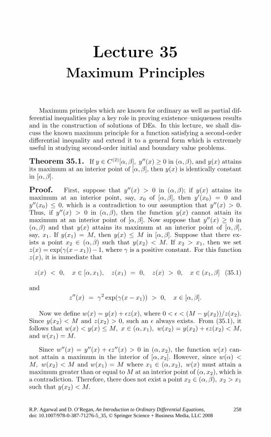
Lecture 35Maximum Principles
Maximum principles which are known for ordinary as well as partial dif-ferential inequalities play a key role in proving existence–uniqueness resultsand in the construction of solutions of DEs. In this lecture, we shall dis-cuss the known maximum principle for a function satisfying a second-orderdifferential inequality and extend it to a general form which is extremelyuseful in studying second-order initial and boundary value problems.
Theorem 35.1. If y ∈ C(2)[α, β], y′′(x) ≥ 0 in (α, β), and y(x) attainsits maximum at an interior point of [α, β], then y(x) is identically constantin [α, β].
Proof. First, suppose that y′′(x) > 0 in (α, β); if y(x) attains itsmaximum at an interior point, say, x0 of [α, β], then y′(x0) = 0 andy′′(x0) ≤ 0, which is a contradiction to our assumption that y′′(x) > 0.Thus, if y′′(x) > 0 in (α, β), then the function y(x) cannot attain itsmaximum at an interior point of [α, β]. Now suppose that y′′(x) ≥ 0 in(α, β) and that y(x) attains its maximum at an interior point of [α, β],say, x1. If y(x1) = M, then y(x) ≤ M in [α, β]. Suppose that there ex-ists a point x2 ∈ (α, β) such that y(x2) < M. If x2 > x1, then we setz(x) = exp(γ(x−x1))− 1, where γ is a positive constant. For this functionz(x), it is immediate that
z(x) < 0, x ∈ [α, x1), z(x1) = 0, z(x) > 0, x ∈ (x1, β] (35.1)
andz′′(x) = γ2 exp(γ(x− x1)) > 0, x ∈ [α, β].
Now we define w(x) = y(x) + εz(x), where 0 < ε < (M − y(x2))/z(x2).Since y(x2) < M and z(x2) > 0, such an ε always exists. From (35.1), itfollows that w(x) < y(x) ≤ M, x ∈ (α, x1), w(x2) = y(x2) + εz(x2) < M,and w(x1) = M.
Since w′′(x) = y′′(x) + εz′′(x) > 0 in (α, x2), the function w(x) can-not attain a maximum in the interior of [α, x2]. However, since w(α) <M, w(x2) < M and w(x1) = M where x1 ∈ (α, x2), w(x) must attain amaximum greater than or equal toM at an interior point of (α, x2), which isa contradiction. Therefore, there does not exist a point x2 ∈ (α, β), x2 > x1such that y(x2) < M.
R.P. Agarwal and D. O’Regan, An Introduction to Ordinary Differential Equations,
258doi: 10.1007/978-0-387-71276-5_35, © Springer Science + Business Media, LLC 2008

Maximum Principles 259
If x2 < x1, we can set z(x) = exp(−γ(x−x1))− 1, where γ is a positiveconstant and again by similar arguments we can show that such an x2cannot exist. Therefore, y(x) = M in [α, β].
The above result holds if we reverse the inequality and replace “maxi-mum” by “minimum.”
We shall now consider a more general inequality y′′+p(x)y′+q(x)y ≥ 0.However, for this inequality the following examples show that no matterwhether q(x) is negative or positive the preceding result need not hold.Hence, we can at most expect a restricted form of maximum principle.
Example 35.1. The function y(x) = sinx is a solution of y′′ + y = 0.However, in the interval [0, π], y(x) attains its maximum at x = π/2 whichis an interior point.
Example 35.2. For y′′ − y = 0, y(x) = −ex − e−x is a solution whichattains its maximum value −2 at x = 0 in the interval [−1, 1].
Theorem 35.2. Let y(x) satisfy the differential inequality
y′′(x) + p(x)y′(x) + q(x)y(x) ≥ 0, x ∈ (α, β) (35.2)
in which p(x) and q(x) (≤ 0) are bounded in every closed subinterval of(α, β). If y(x) assumes a nonnegative maximum value M at an interiorpoint of [α, β], then y(x) ≡ M.
Proof. If the inequality in (35.2) is strict and y(x) assumes a nonnegativemaximum M at an interior point x0 of [α, β], then y(x0) = M, y′(x0) = 0and y′′(x0) ≤ 0. Since p(x) and q(x) are bounded in a closed subintervalcontaining x0 and q(x) ≤ 0, we have
y′′(x0) + p(x0)y′(x0) + q(x0)y(x0) ≤ 0,
contrary to our assumption of strict inequality in (35.2). Hence, if theinequality (35.2) is strict, y(x) cannot attain its nonnegative maximum atan interior point of [α, β].
Now if (35.2) holds and y(x1) = M for some x1 ∈ (α, β), we supposethat there exists a point x2 ∈ (α, β) such that y(x2) < M. If x2 > x1, thenonce again we set z(x) = exp(γ(x−x1)) − 1, where γ is a positive constantyet to be determined. This function z(x) satisfies (35.1), and since q(x) ≤ 0it follows that
z′′ + p(x)z′ + q(x)z
= [γ2 + p(x)γ + q(x)(1 − exp(−γ(x− x1)))] exp(γ(x− x1))
≥ [γ2 + p(x)γ + q(x)] exp(γ(x− x1)).

260 Lecture 35
We choose γ such that γ2+p(x)γ+q(x) > 0 in (α, β). This is always possiblesince p(x) and q(x) are bounded in every closed subinterval of (α, β). Withsuch a choice of γ, we see that
z′′ + p(x)z′ + q(x)z > 0.
The rest of the proof is word for word the same as that of Theorem35.1, except for the function w instead of w′′(x) > 0 we now have w′′(x) +p(x)w′(x) + q(x)w(x) > 0.
If q(x) is not identically zero in (α, β), then the only nonnegative con-stant M for which y(x) = M satisfies (35.2) is M = 0. For this, wehave y(x) = M ≥ 0, y′(x) = y′′(x) = 0, x ∈ (α, β) and thereforey′′(x) + p(x)y′(x) + q(x)y(x) = q(x)M ≥ 0, but q(x) ≤ 0, and hence itis necessary that M = 0.
Next we shall prove the following corollaries.
Corollary 35.3. Suppose that y(x) is a nonconstant solution of thedifferential inequality (35.2) having one-sided derivatives at α and β, andp(x) and q(x) (≤ 0) are bounded in every closed subinterval of (α, β). If y(x)has a nonnegative maximum at α and if the function p(x) + (x − α)q(x)is bounded from below at α, then y′(α) < 0. If y(x) has a nonnegativemaximum at β and if p(x) − (β − x)q(x) is bounded from above at β, theny′(β) > 0.
Proof. Suppose that y(x) has a nonnegative maximum at α, say, y(α) =M ≥ 0, then y(x) ≤ M, x ∈ [α, β], and since y(x) is nonconstant, thereexists a x0 ∈ (α, β) such that y(x0) < M.
We define z(x) = exp(γ(x− α)) − 1, where γ is a positive constant yetto be determined. Then since q(x) ≤ 0 and 1 − exp(−γ(x−α)) ≤ γ(x−α)for x ≥ α it follows that
z′′ + p(x)z′ + q(x)z
= [γ2 + p(x)γ + q(x)(1 − exp(−γ(x− α)))] exp(γ(x− α))
≥ [γ2 + γ(p(x) + q(x)(x− α))] exp(γ(x− α)).
We choose γ such that γ2 +γ(p(x)+q(x)(x−α)) > 0 for x ∈ [α, x0]. This isalways possible since p(x) and q(x) are bounded in every closed subintervaland p(x)+(x−α)q(x) is bounded from below at α. Then z′′+p(x)z′+q(x)z >0.
Now we define w(x) = y(x) + εz(x), where 0 < ε < (M − y(x0))/z(x0).Then w(α) = y(α) = M which implies that w(x) has a maximum greaterthan or equal to M in [α, x0]. However, since w′′ + p(x)w′ + q(x)w > 0,the nonnegative maximum must occur at one of the endpoints of [α, x0].

Maximum Principles 261
Finally, w(x0) = y(x0) + εz(x0) < M implies that the maximum occurs atα. Therefore, the one-sided derivative of w(x) at α cannot be positive, i.e.,w′(α) ≤ 0, and w′(α) = y′(α) + εz′(α) ≤ 0. However, since z′(α) = γ > 0,we must have y′(α) < 0.
If the nonnegative maximum M of y(x) occurs at β, then by similararguments we can show that y′(β) > 0.
Corollary 35.4. Suppose that y(x) is a solution of the differentialinequality (35.2), which is continuous in [α, β] and y(α) ≤ 0, y(β) ≤ 0, andp(x) and q(x) (≤ 0) are bounded in every closed subinterval of (α, β). Theny(x) < 0 in (α, β) unless y(x) = 0 in [α, β].
Proof. If y(x) has a negative maximum, then y(x) < 0 in [α, β]. Oth-erwise, by Theorem 35.2, the nonnegative maximum of y(x) must occur atthe endpoints. However, since y(α) ≤ 0, y(β) ≤ 0 we must have y(x) < 0in (α, β) unless y(x) = 0 in [α, β].
The following two examples illustrate how maximum principles can beapplied to obtain lower and upper bounds for the solutions of DEs whichcannot be solved explicitly.
Example 35.3. Consider the boundary value problem
y′′ − x2y = 0, x ∈ (α, β)
y(α) = γ1, y(β) = γ2(35.3)
for which a unique solution y(x) always exists.
Suppose there exists a function z(x) such that
z′′ − x2z ≤ 0, z(α) ≥ γ1, z(β) ≥ γ2. (35.4)
For such a function z(x), we define w(x) = y(x) − z(x). Clearly, w(x)satisfies
w′′ − x2w ≥ 0, w(α) ≤ 0, w(β) ≤ 0 (35.5)
and hence Corollary 35.4 is applicable, and we find that w(x) ≤ 0 in [α, β],i.e., y(x) ≤ z(x) in [α, β].
Now we shall construct such a function z(x) as follows: we set z1(x) =A2 − exp(−γ(x−α)) where A and γ are constants yet to be determined.Since
z′′1 − x2z1 = A(−γ2 + x2) exp(−γ(x− α)) − 2x2,
we choose A = maxγ1, γ2, 0, and γ = max|α|, |β| + 1, so that A ≥0, γ > 0, − γ2 + x2 < 0, x ∈ [α, β]. Thus, with this choice of A and γ, itfollows that z′′
1 − x2z1 ≤ 0, z1(α) = A ≥ γ1, z1(β) ≥ A ≥ γ2. Hence, z1(x)satisfies (35.4) and we have y(x) ≤ z1(x), x ∈ [α, β].

262 Lecture 35
Similarly, to obtain a lower bound for y(x), we let z2(x) = B2 −exp(−γ(x−α)) where γ is chosen as before and B = minγ1, γ2, 0. ThenB ≤ 0, and z2(x) satisfies z′′
2 − x2z2 ≥ 0, z2(α) = B ≤ γ1, z2(β) ≤B ≤ γ2. Hence, z2(x) satisfies (35.4) with the inequalities reversed, andthe function w(x) = z2(x) − y(x) satisfies (35.5). Therefore, it follows thatz2(x) ≤ y(x), x ∈ [α, β].
In conclusion, we have
Bφ(x) ≤ y(x) ≤ Aφ(x),
where A = maxγ1, γ2, 0, B = minγ1, γ2, 0, φ(x) = 2 − exp(−γ(x−α))and γ = max|α|, |β| + 1.
Example 35.4. Once again we consider the DE y′′ − x2y = 0 in theinterval (0, 1), but with initial conditions y(0) = 1, y′(0) = 0.
To obtain an upper bound for y(x), it suffices to find a function z1(x)satisfying
z′′1 − x2z1 ≥ 0, x ∈ (0, 1), z1(0) ≥ 1, z′
1(0) ≥ 0. (35.6)
For this, we define v1(x) = z1(x) − y(x), and note that
v′′1 − x2v1 ≥ 0, x ∈ (0, 1), v1(0) ≥ 0, v′
1(0) ≥ 0.
Since v1(0) ≥ 0, the function v1(x) has a nonnegative maximum in everysubinterval [0, x0] of [0, 1]. Thus, from Theorem 35.2 it follows that thismaximum must occur either at 0 or x0. Since v′
1(0) ≥ 0, from Corollary35.3, the maximum must occur at x0 unless v1(x) is constant in [0, x1].Hence, for x0 ∈ (0, 1), v1(x0) ≥ v1(0) ≥ 0, and by Corollary 35.3 we findthat v′
1(x0) ≥ 0. Therefore, it follows that for each x ∈ (0, 1), v1(x) =z1(x) − y(x) ≥ v1(0) ≥ 0, and hence y(x) ≤ z1(x).
To construct such a function z1(x), we set z1(x) = c1x2 + 1, where c1 is
a constant yet to be determined. Since
z′′1 − x2z1 = 2c1 − x2(c1x2 + 1) = c1(2 − x4) − x2
we need to choose c1 such that c1 ≥ x2/(2 − x4), x ∈ [0, 1]. Since x2/(2 −x4) ≤ 1 for all x ∈ [0, 1], we can let c1 = 1. Then z1(x) = x2 + 1 and itsatisfies (35.6). Therefore, it follows that y(x) ≤ x2 + 1, x ∈ [0, 1].
Similarly, to obtain a lower bound we need to find a function z2(x)satisfying
z′′2 − x2z2 ≤ 0, x ∈ (0, 1), z2(0) ≤ 1, z′
2(0) ≤ 0. (35.7)
To construct such a function z2(x), once again we set z2(x) = c2x2 + 1,
where c2 is a constant yet to be determined. Since
z′′2 − x2z2 = c2(2 − x4) − x2

Maximum Principles 263
we need to choose c2 such that c2 ≤ x2/(2 − x4), x ∈ [0, 1]. Therefore, wecan choose c2 = 0, to obtain z2(x) = 1 which satisfies (35.7). Hence, itfollows that 1 ≤ y(x), x ∈ [0, 1].
In conclusion, we have
1 ≤ y(x) ≤ 1 + x2, x ∈ [0, 1].
Finally, we remark that in Examples 35.3 and 35.4 above we can usepolynomials, rational functions, exponentials, etc., for the construction ofthe functions z1(x) and z2(x).
Problems
35.1. The function y = sinx, x ∈ (0, π) attains its positive maximumat x = π/2, and is a solution of the DE
y′′ + (tanx)y′ = 0.
Does this contradict Theorem 35.2?
35.2. Consider the DE
y′′ + αeβy = − x2, x ∈ (0, 1),
where α and β are positive constants. Show that its solution cannot attaina minimum in (0, 1).
35.3. Consider the DE
y′′ − α cos(y′) = βx4, x ∈ (−1, 1),
where α and β are positive constants. Show that its solution cannot attaina maximum in (−1, 1).
35.4. Consider the boundary value problem
y′′ + x2y′ = − x4, x ∈ (0, 1)
y(0) = 0 = y(1).
Show that its solution cannot attain a minimum in (0, 1). Further, showthat y′(0) > 0, y′(1) < 0.
35.5. Show that the boundary value problem
y′′ + p(x)y′ + q(x)y = r(x), x ∈ (α, β)
y(α) = A, y(β) = B

264 Lecture 35
where p(x) and q(x) are as in Theorem 35.2, has at most one solution.
35.6. Show that the solution y(x) of the boundary value problem
y′′ − xy = 0, x ∈ (0, 1), y(0) = 0, y(1) = 1
satisfies the inequalities (x+ x2)/2 ≤ y(x) ≤ x, x ∈ [0, 1].
35.7. Show that the solution y(x) of the initial value problem
y′′ +1xy′ − y = 0, x ∈ (0, 1), y(0) = 1, y′(0) = 0
satisfies the inequalities 1 + x2/4 ≤ y(x) ≤ 1 + x2/3, x ∈ [0, 1].
Answers or Hints
35.1. No.
35.2. Use contradiction.
35.3. Use contradiction.
35.4. Use contradiction.
35.5. Use Corollary 35.4.
35.6. See Example 35.3.
35.7. See Example 35.4.

Lecture 36Sturm–Liouville Problems
In our previous lectures we have seen that homogeneous boundary valueproblem (6.1), (32.2) may have nontrivial solutions. If the coefficients ofthe DE and/or of the boundary conditions depend upon a parameter, thenone of the pioneer problems of mathematical physics is to determine thevalue(s) of the parameter for which such nontrivial solutions exist. Thesespecial values of the parameter are called eigenvalues and the correspondingnontrivial solutions are called eigenfunctions. The boundary value problemwhich consists of the self-adjoint DE
(p(x)y′)′ + q(x)y + λr(x)y = P2[y] + λr(x)y = 0 (36.1)
and the boundary conditions (33.14) is called the Sturm–Liouville problem.In the DE (36.1), λ is a parameter, and the functions q, r ∈ C(J), p ∈C1(J), and p(x) > 0, r(x) > 0 in J.
The problem (36.1), (33.14) satisfying the above conditions is said to bea regular Sturm–Liouville problem. Solving such a problem means findingvalues of λ (eigenvalues) and the corresponding nontrivial solutions φλ(x)(eigenfunctions). The set of all eigenvalues of a regular problem is calledits spectrum.
The computation of eigenvalues and eigenfunctions is illustrated in thefollowing examples.
Example 36.1. Consider the boundary value problem
y′′ + λy = 0 (36.2)
y(0) = y(π) = 0. (36.3)
If λ = 0, then the general solution of (36.2) is y(x) = c1 + c2x, and thissolution satisfies the boundary conditions (36.3) if and only if c1 = c2 = 0,i.e., y(x) ≡ 0 is the only solution of (36.2), (36.3). Hence, λ = 0 is not aneigenvalue of the problem (36.2), (36.3).
If λ = 0, it is convenient to replace λ by µ2, where µ is a new parameternot necessarily real. In this case the general solution of (36.2) is y(x) =c1e
iµx + c2e−iµx, and this solution satisfies the boundary conditions (36.3)
if and only ifc1 + c2 = 0
c1eiµπ + c2e
−iµπ = 0.(36.4)
R.P. Agarwal and D. O’Regan, An Introduction to Ordinary Differential Equations,
doi: 10.1007/978-0-387-71276-5_36, © Springer Science + Business Media, LLC 2008
265

266 Lecture 36
The system (36.4) has a nontrivial solution if and only if
e−iµπ − eiµπ = 0. (36.5)
If µ = a+ ib, where a and b are real, condition (36.5) reduces to
ebπ(cos aπ − i sin aπ) − e−bπ(cos aπ + i sin aπ)
= (ebπ − e−bπ) cos aπ − i(ebπ + e−bπ) sin aπ
= 2 sinh bπ cos aπ − 2i cosh bπ sin aπ = 0,
i.e.,sinh bπ cos aπ = 0 (36.6)
andcosh bπ sin aπ = 0. (36.7)
Since cosh bπ > 0 for all values of b, equation (36.7) requires that a = n,where n is an integer. Further, for this choice of a, cos aπ = 0, and equation(36.6) reduces to sinh bπ = 0, i.e., b = 0. However, if b = 0, then wecannot have a = 0, because then µ = 0, and we have seen that it is notan eigenvalue. Hence, µ = n, where n is a nonzero integer. Thus, theeigenvalues of (36.2), (36.3) are λn = µ2 = n2, n = 1, 2, . . . . Further, from(36.4) since c2 = −c1 for λn = n2 the corresponding nontrivial solutions ofthe problem (36.2), (36.3) are
φn(x) = c1(einx − e−inx) = 2ic1 sinnx,
or, simply φn(x) = sinnx.
Example 36.2. Consider again the DE (36.2), but with the boundaryconditions
y(0) + y′(0) = 0, y(1) = 0. (36.8)
If λ = 0, then the general solution y(x) = c1 +c2x of (36.2) also satisfiesthe boundary conditions (36.8) if and only if c1 + c2 = 0, i.e., c2 = −c1.Hence, λ = 0 is an eigenvalue of (36.2), (36.8) and the corresponding eigen-function is φ1(x) = 1 − x.
If λ = 0, then once again we replace λ by µ2 and note that the generalsolution y(x) = c1e
iµx + c2e−iµx of (36.2) satisfies the boundary conditions
(36.8) if and only if
(c1 + c2) + iµ(c1 − c2) = 0
c1eiµ + c2e
−iµ = 0.(36.9)
The system (36.9) has a nontrivial solution if and only if
(1 + iµ)e−iµ − (1 − iµ)eiµ = 0,

Sturm–Liouville Problems 267
which is equivalent totanµ = µ. (36.10)
To find the real roots of (36.10) we graph the curves y = µ and y = tanµand observe the values of µ where these curves intersect.
µ
y
1 2 3 4 5 6 7 8
2
4
6
8
10
12
14
π2
3π2
5π2
Figure 36.1
From Figure 36.1 it is clear that the equation (36.10) has an infinitenumber of positive roots µn, n = 1, 2, . . . , which are approaching the oddmultiples of π/2, i.e., µn (2n+1)π/2. Further, since the equation (36.10)remains unchanged if µ is replaced by −µ, we find that the only nonzeroreal roots of (36.10) are µn ±(2n+ 1)π/2, n = 1, 2, . . . .
Thus, the problem (36.2), (36.8) also has an infinite number of eigenval-ues, λ1 = 0, λn+1 (2n+1)2π2/4, n = 1, 2, . . . . Further, from (36.9) sincec2 = −c1e2iµ for these λn, n > 1 the corresponding nontrivial solutions ofthe problem (36.2), (36.8) are
y(x) = c1ei√
λnx − c1e−i
√λnxe2i
√λn = − 2c1iei
√λn sin
√λn(1 − x).
Hence, the eigenfunctions of (36.2), (36.8) are
φ1(x) = 1 − xφn(x) = sin
√λn(1 − x), n = 2, 3, . . . .

268 Lecture 36
From Example 36.1 it is clear that the problem (36.2), (36.3) has aninfinite number of real eigenvalues λn, which can be arranged as a mono-tonic increasing sequence λ1 < λ2 < · · · such that λn → ∞ as n → ∞.Also, corresponding to each eigenvalue λn of (36.2), (36.3) there exists aone-parameter family of eigenfunctions φn(x), which has exactly (n−1) ze-ros in the open interval (0, π). Further, these eigenfunctions are orthogonal.This concept is defined in the following definition.
Definition 36.1. The set of functions φn(x) : n = 0, 1, . . . each ofwhich is piecewise continuous in an infinite or a finite interval [α, β] is saidto be orthogonal in [α, β] with respect to the nonnegative function r(x) if
(φm, φn) =∫ β
α
r(x)φm(x)φn(x)dx = 0 for all m = n
and ∫ β
α
r(x)φ2n(x)dx = 0 for all n.
The function r(x) is called the weight function. In what follows we shallassume that the function r(x) has only a finite number of zeros in [α, β]and the integrals
∫ β
αr(x)φn(x)dx, n = 0, 1, . . . exist.
The orthogonal set φn(x) : n = 0, 1, . . . in [α, β] with respect to theweight function r(x) is said to be orthonormal if
∫ β
α
r(x)φ2n(x)dx = 1 for all n.
Thus, orthonormal functions have the same properties as orthogonal func-tions, but, in addition, they have been normalized, i.e., each function φn(x)of the orthogonal set has been divided by the norm of that function, whichis defined as
‖φn‖ =
(∫ β
α
r(x)φ2n(x)dx
)1/2
.
Now since ∫ π
0sin kx sin xdx = 0,
for all k = , the set of eigenfunctions φn(x) = sinnx, n = 1, 2, . . . of(36.2), (36.3) is orthogonal in [0, π] with the weight function r(x) = 1.
Clearly, the above properties of eigenvalues and eigenfunctions of (36.2),(36.3) are also valid for the problem (36.2), (36.8). In fact, these propertieshold for the general regular Sturm–Liouville problem (36.1), (33.14). Weshall state these properties as theorems and prove the results.

Sturm–Liouville Problems 269
Theorem 36.1. The eigenvalues of the regular Sturm–Liouville prob-lem (36.1), (33.14) are simple, i.e., if λ is an eigenvalue of (36.1), (33.14)and φ1(x) and φ2(x) are the corresponding eigenfunctions, then φ1(x) andφ2(x) are linearly dependent.
Proof. Since φ1(x) and φ2(x) both are solutions of (36.1), from (30.23)it follows that p(x)W (φ1, φ2)(x) = c (constant). To find the value of c, wenote that φ1 and φ2 satisfy the boundary conditions, and hence
a0φ1(α) + a1φ′1(α) = 0
a0φ2(α) + a1φ′2(α) = 0,
which implies W (φ1, φ2)(α) = 0, and hence c is zero. Thus, p(x)W (φ1,φ2)(x) ≡ 0, i.e., φ1(x) and φ2(x) are linearly dependent.
Theorem 36.2. Let λn, n = 1, 2, . . . be the eigenvalues of the reg-ular Sturm–Liouville problem (36.1), (33.14) and φn(x), n = 1, 2, . . . bethe corresponding eigenfunctions. Then the set φn(x) : n = 1, 2, · · · isorthogonal in [α, β] with respect to the weight function r(x).
Proof. Let λk and λ, (k = ) be eigenvalues, and φk(x) and φ(x) bethe corresponding eigenfunctions of (36.1), (33.14). Since φk(x) and φ(x)are solutions of (36.1), we have
P2[φk] + λkr(x)φk(x) = 0
andP2[φ] + λr(x)φ(x) = 0.
Thus, from Green’s identity (30.24) it follows that
(λ − λk)∫ β
α
r(x)φk(x)φ(x)dx =∫ β
α
(φP2[φk] − φkP2[φ])dx
= p(x)[φ(x)φ′k(x) − φ′
(x)φk(x)]∣∣∣βα.
(36.11)Next since φk(x) and φ(x) satisfy the boundary conditions (33.14), i.e.,
a0φk(α) + a1φ′k(α) = 0, d0φk(β) + d1φ
′k(β) = 0
a0φ(α) + a1φ′(α) = 0, d0φ(β) + d1φ
′(β) = 0
it is necessary that
φk(α)φ′(α) − φ′
k(α)φ(α) = φk(β)φ′(β) − φ′
k(β)φ(β) = 0.
Hence, the identity (36.11) reduces to
(λ − λk)∫ β
α
r(x)φk(x)φ(x)dx = 0. (36.12)

270 Lecture 36
However, since λ = λk, it follows that
∫ β
α
r(x)φk(x)φ(x)dx = 0.
Corollary 36.3. Let λ1 and λ2 be two eigenvalues of the regularSturm–Liouville problem (36.1), (33.14) and φ1(x) and φ2(x) be the cor-responding eigenfunctions. Then φ1(x) and φ2(x) are linearly dependentonly if λ1 = λ2.
Proof. The proof is a direct consequence of equality (36.12).
Theorem 36.4. For the regular Sturm–Liouville problem (36.1),(33.14) eigenvalues are real.
Proof. Let λ = a+ ib be a complex eigenvalue and φ(x) = µ(x) + iν(x)be the corresponding eigenfunction of (36.1), (33.14). Then we have
(p(x)(µ+ iν)′)′ + q(x)(µ+ iν) + (a+ ib)r(x)(µ+ iν) = 0
and henceP2[µ] + (aµ(x) − bν(x))r(x) = 0
P2[ν] + (bµ(x) + aν(x))r(x) = 0
a0µ(α) + a1µ′(α) = 0, d0µ(β) + d1µ
′(β) = 0
anda0ν(α) + a1ν
′(α) = 0, d0ν(β) + d1ν′(β) = 0.
Thus, as in Theorem 36.2, we find
∫ β
α
(νP2[µ] − µP2[ν])dx
=∫ β
α
[−(aµ(x) − bν(x))ν(x)r(x) + (bµ(x) + aν(x))µ(x)r(x)]dx
= b
∫ β
α
(ν2(x) + µ2(x))r(x)dx
= p(x)(νµ′ − ν′µ)∣∣∣βα
= 0.
Hence, it is necessary that b = 0, i.e., λ is real.
Since (36.2), (36.8) is a regular Sturm–Liouville problem, from Theorem36.4 it is immediate that the equation (36.10) has only real roots.

Lecture 37
Sturm–Liouville Problems(Contd.)
In Lecture 36 we have established several properties of the eigenvaluesand eigenfunctions of the regular Sturm–Liouville problem (36.1), (33.14).In all these results the existence of eigenvalues is tacitly assumed. We nowstate and prove the following important result.
Theorem 37.1. For the regular Sturm–Liouville problem (36.1),(33.14) there exists an infinite number of eigenvalues λn, n = 1, 2, . . . .These eigenvalues can be arranged as a monotonic increasing sequenceλ1 < λ2 < · · · such that λn → ∞ as n → ∞. Further, eigenfunctionφn(x) corresponding to the eigenvalue λn has exactly (n − 1) zeros in theopen interval (α, β).
Proof. We shall establish this result first for the particular problem(36.1),
y(α) = y(β) = 0. (37.1)For this, we observe the following:
(i) If eigenvalues of (36.1), (37.1) exist, then these are all real numbers(cf. Theorem 36.4).(ii) For each fixed λ there exists a unique solution y(x, λ) of the initialvalue problem (36.1),
y(α, λ) = 0, y′(α, λ) = 1. (37.2)
Further, y(x, λ) as well as y′(x, λ) vary continuously with λ (cf. Theo-rem 16.8).
(iii) There exist constants p, P, q, Q, r, and R such that for all x ∈[α, β], 0 < p ≤ p(x) ≤ P , q ≤ q(x) ≤ Q, and 0 < r ≤ r(x) ≤ R. Thus, fora fixed λ > 0 the solution y(x, λ) of (36.1), (37.2) oscillates more rapidlythan the solution y0(x, λ) of the problem
(Py′0)
′ + qy0 + λry0 = 0
y0(α, λ) = 0, y′0(α, λ) = 1
(37.3)
and less rapidly than the solution y1(x, λ) of the problem
(py′1)
′ +Qy1 + λRy1 = 0
y1(α, λ) = 0, y′1(α, λ) = 1
(37.4)
R.P. Agarwal and D. O’Regan, An Introduction to Ordinary Differential Equations,
doi: 10.1007/978-0-387-71276-5_37, © Springer Science + Business Media, LLC 2008
271

272 Lecture 37
(cf. Theorem 31.4). When λ is negative, r and R in (37.3) and (37.4) needto be interchanged.
The problems (37.3) and (37.4) are with constant coefficients (modifiedas indicated when λ is negative), and hence can be solved explicitly. Ifλ > 0 is so large that 0 < (q+λr)/P = a2, then the solution of the problem(37.3) is y0(x) = (1/a) sin a(x−α), which vanishes at least once in the openinterval (α, β) provided a(β−α) > π, i.e., (q+λr)/P > π2/(β−α)2. Thus,for each
λ > max
0,1r
(Pπ2
(β − α)2− q
)= λ0
the solution of the problem (36.1), (37.2) has at least one zero in (α, β).Similarly, if λ < 0 is so small that
−a2 =Q+ λr
P< 0, i.e., λ < min
0, − Q
r
= λ1,
then the solution of the modified problem (37.4) is y(x) = (1/a) sinh a(x−α), which does not vanish again at x = β or, indeed, anywhere else. Hence,for each λ < λ1 the solution of the problem (36.1), (37.2) has no zero inthe interval (α, β]. Now since the solution y(x, λ) of (36.1), (37.2) variescontinuously with λ, if y(x, λ) has a zero in (α, β), then its position alsovaries continuously with λ. Thus, if λ increases steadily from λ1 (for whichthe solution of (36.1), (37.2) has no zero in (α, β]) towards λ0, then therewill be a specific value of λ, say, λ1, for which y(x, λ) first vanishes atx = β. This proves that there exists a smallest eigenvalue λ1 of the problem(36.1), (37.1) and y(x, λ1) the solution of (36.1), (37.2) is the correspondingeigenfunction. By allowing λ to increase from the value λ1 one argues thatthere is a number λ2 > λ1 for which y(x, λ2), the solution of (36.1), (37.2)has precisely one zero in (α, β) and y(β, λ2) = 0. As λ continues to increasethere results a sequence of eigenvalues λ1 < λ2 < · · · and a correspondingsequence of eigenfunctions y(x, λ1), y(x, λ2), . . . . Further, y(x, λn) will haveprecisely (n− 1) zeros in the open interval (α, β). This completes the proofof Theorem 37.1 for the problem (36.1), (37.1).
Next for the problem (36.1),
a0y(α) + a1y′(α) = 0, y(β) = 0 (37.5)
we note that the above proof holds if the solution y(x, λ) of (36.1), (37.2)is replaced by the solution z(x, λ) of the initial value problem (36.1),
z(α, λ) = a1, z′(α, λ) = − a0. (37.6)
Thus, the problem (36.1), (37.5) also has a sequence of eigenvalues λ′1 <
λ′2 < · · · and a corresponding sequence of eigenfunctions z(x, λ′
1), z(x, λ′2),
· · · such that z(x, λ′n) has precisely (n−1) zeros in the open interval (α, β).

Sturm–Liouville Problems (Contd.) 273
Finally, we shall consider the problem (36.1), (33.14). For the solu-tion z(x, λ) of (36.1), (37.6), Theorem 16.8 implies that ∂z(x, λ)/∂λ is thesolution of the initial value problem
P2
[∂
∂λz(x, λ)
]+ λ r(x)
∂
∂λz(x, λ) + r(x)z(x, λ) = 0
∂
∂λz(α, λ) =
∂
∂λz′(α, λ) = 0.
Thus, from Green’s identity (30.24) it follows that∫ β
α
(∂
∂λz(x, λ)P2[z(x, λ)] − z(x, λ)P2
[∂
∂λz(x, λ)
])dx
=∫ β
α
r(x)z2(x, λ)dx
=(p(x)
(∂
∂λz(x, λ)z′(x, λ) − ∂
∂λz′(x, λ)z(x, λ)
))∣∣∣∣β
α
= p(β)W(∂
∂λz(β, λ), z(β, λ)
);
i.e.,
W
(∂
∂λz(β, λ), z(β, λ)
)> 0.
Now in the interval (λ′n, λ
′n+1) we know that z(β, λ) = 0, thus for all
λ ∈ (λ′n, λ
′n+1) the function φ(λ) = z′(β, λ)/z(β, λ) is well defined. Further,
since
φ′(λ) = − W(
∂∂λz(β, λ), z(β, λ)
)z2(β, λ)
it follows that φ′(λ) < 0, i.e., in the interval (λ′n, λ
′n+1) the function φ(λ)
monotonically decreases. Also, since z(β, λ′n) = z(β, λ′
n+1) = 0, z′(β, λ′n) =
0, and z′(β, λ′n+1) = 0, it is necessary that φ(λ′
n) = ∞, and φ(λ′n+1) = −∞,
i.e., φ(λ) monotonically decreases from +∞ to −∞. Therefore, there existsa unique λ′′
n ∈ (λ′n, λ
′n+1) such that
z′(β, λ′′n)
z(β, λ′′n)
= − d0
d1.
Hence, for the problem (36.1), (33.14) there exists a sequence of eigenvaluesλ′′
1 < λ′′2 < · · · such that λ′′
n ∈ (λ′n, λ
′n+1), and z(x, λ′′
n), n = 1, 2, . . . are thecorresponding eigenfunctions. Obviously, z(x, λ′′
n) has exactly (n− 1) zerosin (α, β).
Now we shall give some examples of singular Sturm–Liouville problemswhich show that the properties of eigenvalues and eigenfunctions for regularproblems do not always hold.

274 Lecture 37
Example 37.1. For the singular Sturm–Liouville problem (36.2),
y(0) = 0, |y(x)| ≤ M < ∞ for all x ∈ (0,∞) (37.7)
each λ ∈ (0,∞) is an eigenvalue and sin√λx is the corresponding eigenfunc-
tion. Thus, in comparison with the regular problems where the spectrumis always discrete, the singular problems may have continuous spectrum.
Example 37.2. Consider the singular Sturm–Liouville problem (36.2),
y(−π) = y(π), y′(−π) = y′(π). (37.8)
This problem has eigenvalues λ1 = 0, λn+1 = n2, n = 1, 2, . . . . The eigen-value λ1 = 0 is simple and 1 is its corresponding eigenfunction. The eigen-value λn+1 = n2, n ≥ 1 is not simple and two independent eigenfunctionsare sinnx and cosnx. Thus, in contrast with regular problems where theeigenvalues are simple, there may be multiple eigenvalues for singular prob-lems.
Finally, we remark that the properties of the eigenvalues and eigenfunc-tions of regular Sturm–Liouville problems can be extended under appro-priate assumptions to singular problems also in which the function p(x) iszero at α or β, or both, but remains positive in (α, β). This case includes,in particular, the following examples.
Example 37.3. Consider the singular Sturm–Liouville problem
(1 − x2)y′′ − 2xy′ + λy = ((1 − x2)y′)′ + λy = 0 (37.9)
limx→−1
y(x) < ∞, limx→1
y(x) < ∞. (37.10)
The eigenvalues of this problem are λn = n(n − 1), n = 1, 2, . . . and thecorresponding eigenfunctions are the Legendre polynomials Pn−1(x) whichin terms of Rodrigues’ formula are defined by
Pn(x) =1
2n (n)!dn
dxn(x2 − 1)n, n = 0, 1, . . . . (37.11)
Example 37.4. Consider the singular Sturm–Liouville problem (37.9),
y′(0) = 0, limx→1
y(x) < ∞. (37.12)
The eigenvalues of this problem are λn = (2n − 2)(2n − 1), n = 1, 2, . . .and the corresponding eigenfunctions are the even Legendre polynomialsP2n−2(x).Example 37.5. Consider the singular Sturm–Liouville problem (37.9),
y(0) = 0, limx→1
y(x) < ∞. (37.13)

Sturm–Liouville Problems (Contd.) 275
The eigenvalues of this problem are λn = (2n−1)(2n), n = 1, 2, . . . and thecorresponding eigenfunctions are the odd Legendre polynomials P2n−1(x).
Example 37.6. Consider the singular Sturm–Liouville problem
y′′ − 2xy′ + λy = 0 =(e−x2
y′)′
+ λe−x2y (37.14)
limx→−∞
y(x)|x|k < ∞, lim
x→∞y(x)xk
< ∞ for some positive integer k.
(37.15)The eigenvalues of this problem are λn = 2(n − 1), n = 1, 2, . . . and thecorresponding eigenfunctions are the Hermite polynomials Hn−1(x) whichin terms of Rodrigues’ formula are defined by
Hn(x) = (−1)nex2 dn
dxne−x2
, n = 0, 1, . . . . (37.16)
Example 37.7. Consider the singular Sturm–Liouville problem
xy′′ + (1 − x)y′ + λy = 0 =(xe−xy′)′ + λe−xy (37.17)
limx→0
|y(x)| < ∞, limx→∞
y(x)xk
< ∞ for some positive integer k.
(37.18)The eigenvalues of this problem are λn = n − 1, n = 1, 2, . . . and thecorresponding eigenfunctions are the Laguerre polynomials Ln−1(x) whichin terms of Rodrigues’ formula are defined by
Ln(x) =ex
n!dn
dxn
(xne−x
). (37.19)
Problems
37.1. Show that the set 1, cosnx, n = 1, 2, . . . is orthogonal on [0, π]with r(x) = 1.
37.2. Show that the set√
2π sinnx, n = 1, 2, . . .
is orthonormal on
[0, π] with r(x) = 1.
37.3. Show that the set
1√2π, 1√
πcosnx, 1√
πsinnx, n = 1, 2, . . .
is
orthonormal on [−π, π] with r(x) = 1.
37.4. Show that the substitution x = cos θ transforms the Cheby-shev DE
(1 − x2)y′′ − xy′ + n2y = 0 (37.20)
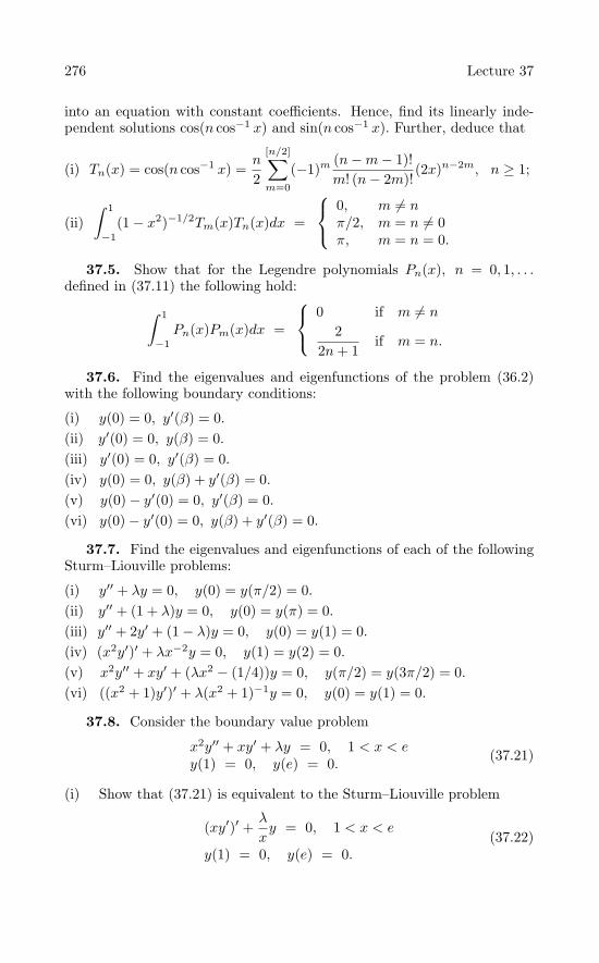
276 Lecture 37
into an equation with constant coefficients. Hence, find its linearly inde-pendent solutions cos(n cos−1 x) and sin(n cos−1 x). Further, deduce that
(i) Tn(x) = cos(n cos−1 x) =n
2
[n/2]∑m=0
(−1)m (n−m− 1)!m! (n− 2m)!
(2x)n−2m, n ≥ 1;
(ii)∫ 1
−1(1 − x2)−1/2Tm(x)Tn(x)dx =
⎧⎨⎩
0, m = nπ/2, m = n = 0π, m = n = 0.
37.5. Show that for the Legendre polynomials Pn(x), n = 0, 1, . . .defined in (37.11) the following hold:
∫ 1
−1Pn(x)Pm(x)dx =
⎧⎨⎩
0 if m = n
22n+ 1
if m = n.
37.6. Find the eigenvalues and eigenfunctions of the problem (36.2)with the following boundary conditions:
(i) y(0) = 0, y′(β) = 0.(ii) y′(0) = 0, y(β) = 0.(iii) y′(0) = 0, y′(β) = 0.(iv) y(0) = 0, y(β) + y′(β) = 0.(v) y(0) − y′(0) = 0, y′(β) = 0.(vi) y(0) − y′(0) = 0, y(β) + y′(β) = 0.
37.7. Find the eigenvalues and eigenfunctions of each of the followingSturm–Liouville problems:
(i) y′′ + λy = 0, y(0) = y(π/2) = 0.(ii) y′′ + (1 + λ)y = 0, y(0) = y(π) = 0.(iii) y′′ + 2y′ + (1 − λ)y = 0, y(0) = y(1) = 0.(iv) (x2y′)′ + λx−2y = 0, y(1) = y(2) = 0.(v) x2y′′ + xy′ + (λx2 − (1/4))y = 0, y(π/2) = y(3π/2) = 0.(vi) ((x2 + 1)y′)′ + λ(x2 + 1)−1y = 0, y(0) = y(1) = 0.
37.8. Consider the boundary value problem
x2y′′ + xy′ + λy = 0, 1 < x < ey(1) = 0, y(e) = 0. (37.21)
(i) Show that (37.21) is equivalent to the Sturm–Liouville problem
(xy′)′ +λ
xy = 0, 1 < x < e
y(1) = 0, y(e) = 0.(37.22)

Sturm–Liouville Problems (Contd.) 277
(ii) Verify that for (37.22) the eigenvalues are λn = n2π2, n = 1, 2, . . .and the corresponding eigenfunctions are φn(x) = sin(nπ lnx).(iii) Show that ∫ e
1
1xφm(x)φn(x)dx =
0, m = n1/2, m = n.
37.9. Verify that for the Sturm–Liouville problem
(xy′)′ +λ
xy = 0, 1 < x < e2π
y′(1) = 0, y′(e2π) = 0
the eigenvalues are λn = n2/4, n = 0, 1, . . . and the corresponding eigen-functions are φn(x) = cos
(n ln x
2
). Show that
∫ e2π
1
1xφm(x)φn(x)dx = 0, m = n.
37.10. Consider Mathieu’s DE (see Example 20.1)
y′′ + (λ+ 16d cos 2x)y = 0, 0 ≤ x ≤ π
together with the periodic boundary conditions
y(0) = y(π), y′(0) = y′(π).
Show that the eigenfunctions of this problem are orthogonal.
37.11. Consider the DE
x4y′′ + k2y = 0. (37.23)
(i) Verify that the general solution of (37.23) is
y(x) = x
(A cos
k
x+B sin
k
x
).
(ii) Find the eigenvalues and eigenfunctions of the Sturm–Liouville prob-lem (37.23), y(α) = y(β) = 0, 0 < α < β.
37.12. Show that the problem
y′′ − 4λy′ + 4λ2y = 0, y(0) = 0, y(1) + y′(1) = 0
has only one eigenvalue, and find the corresponding eigenfunction.

278 Lecture 37
37.13. Show that for the singular Sturm–Liouville problem (36.1),(32.7) with p(α) = p(β) eigenfunctions corresponding to different eigen-values are orthogonal in [α, β] with respect to the weight function r(x).
37.14. Solve the following singular Sturm–Liouville problems
(i) y′′ + λy = 0, y′(0) = 0, |y(x)| < ∞ for all x ∈ (0,∞)(ii) y′′ + λy = 0, |y(x)| < ∞ for all x ∈ (−∞,∞).
Answers or Hints
37.1. Verify directly.
37.2. Verify directly.
37.3. Verify directly.
37.4. Equation (37.20) reduces to d2ydθ2 + n2y = 0. (i) Use induction and
the identitycos((n+1) cos−1 x)+cos((n−1) cos−1 x) = 2 cos(n cos−1 x) cos(cos−1 x),
i.e., Tn+1(x) = 2xTn(x) − Tn−1(x). (ii) Use x = cos θ.
37.5. From (37.11) it follows that
2n n!∫ 1
−1 Pm(x)Pn(x)dx =∫ 1
−1 Pm(x) dn
dxn (x2 − 1)ndx
= − ∫ 1−1
ddxPm(x) dn−1
dxn−1 (x2 − 1)ndx.
37.6. (i)(
2n−12β
)2π2, sin
(2n−12β
)πx. (ii)
(2n−12β
)2π2, cos
(2n−12β
)πx
(iii)(
n−1β
)2π2, cos
(n−1
β
)πx. (iv) λ2
n, where λ = λn is a solution of
tanλβ + λ = 0, sinλnx. (v) λ2n, where λ = λn is a solution of cotλβ =
λ, sinλnx + λn cosλnx. (vi) λ2n, where λ = λn is a solution of tanλβ =
2λ/(λ2 − 1), sinλnx+ λn cosλnx.
37.7. (i) 4n2, sin 2nx. (ii) n2 − 1, sinnx. (iii) −n2π2, e−x sinnπx.(iv) 4n2π2, sin 2nπ
(1 − 1
x
). (v) n2, 1√
xsinn
(x− π
2
). (vi) 16n2,
sin(4n tan−1 x).
37.8. Verify directly.
37.9. Verify directly.
37.10. Follow the proof of Theorem 36.2.
37.11. (i) Verify directly. (ii) kn = nπαββ−α , x sin
[nπβ(x−α)
x(β−α)
].
37.12. −1, xe−2x.
37.13. Use (36.11).
37.14. (i) λ ≥ 0, φ(x) = cos√λx. (ii) λ ≥ 0, φ(x) = c1 cos
√λx +
c2 sin√λx.

Lecture 38Eigenfunction Expansions
The basis e1, . . . , en (ek is the unit vector) of IRn has an importantcharacteristic, namely, for every u ∈ IRn there is a unique choice of constantsα1, . . . , αn for which
u =n∑
i=1
αiei.
Further, from the orthonormality of the vectors ei, 1 ≤ i ≤ n we candetermine αi, 1 ≤ i ≤ n as follows:
< u , ej > =
⟨n∑
i=1
αiei , ej
⟩=
n∑i=1
αi < ei , ej > = αj , 1 ≤ j ≤ n.
Thus, the vector u has a unique representation
u =n∑
i=1
< u , ei > ei.
A natural generalization of this result which is widely applicable andhas led to a vast amount of advanced mathematics can be stated as follows:Let φn(x), n = 0, 1, 2, . . . be an orthogonal set of functions in the interval[α, β] with respect to the weight function r(x). Then an arbitrary functionf(x) can be expressed as an infinite series involving orthogonal functionsφn(x), n = 0, 1, 2, . . . as
f(x) =∞∑
n=0
cnφn(x). (38.1)
It is natural to ask the meaning of equality in (38.1), i.e., the type ofconvergence, if any, of the infinite series on the right so that we will havesome idea as to how well this represents f(x). We shall also determine theconstant coefficients cn, n = 0, 1, 2, . . . in (38.1).
Let us first proceed formally without considering the question of con-vergence. We multiply (38.1) by r(x)φm(x) and integrate from α to β, toobtain ∫ β
α
r(x)φm(x)f(x)dx =∫ β
α
∞∑n=0
cnr(x)φn(x)φm(x)dx.
R.P. Agarwal and D. O’Regan, An Introduction to Ordinary Differential Equations,
doi: 10.1007/978-0-387-71276-5_38, © Springer Science + Business Media, LLC 2008
279

280 Lecture 38
Now assuming that the operations of integration and summation on theright of the above equality can be interchanged, we find∫ β
α
r(x)φm(x)f(x)dx =∞∑
n=0
cn
∫ β
α
r(x)φm(x)φn(x)dx
= cm
∫ β
α
r(x)φ2m(x)dx = cm‖φm‖2.
Thus, under suitable convergence conditions, the constant coefficients cn,n = 0, 1, 2, . . . are given by the formula
cn =∫ β
α
r(x)φn(x)f(x)dx
/‖φn‖2. (38.2)
However, if the set φn(x) is orthonormal, so that ‖φn‖ = 1, then we have
cn =∫ β
α
r(x)φn(x)f(x)dx. (38.3)
If the series∑∞
n=0 cnφn(x) converges uniformly to f(x) in [α, β], thenthe above formal procedure is justified, and then the coefficients cn aregiven by (38.2).
The coefficients cn obtained in (38.2) are called the Fourier coefficientsof the function f(x) with respect to the orthogonal set φn(x) and theseries
∑∞n=0 cnφn(x) with coefficients (38.2) is called the Fourier series of
f(x).
We shall write
f(x) ∼∞∑
n=0
cnφn(x)
which, in general, is just a correspondence, i.e., often f(x) = ∑∞n=0 cnφn(x),
unless otherwise proved.
Example 38.1. In Problem 37.5 we have seen that the set of Legendrepolynomials φn(x) = Pn(x), n = 0, 1, . . . is orthogonal on [−1, 1] withr(x) = 1. Also,
‖Pn‖2 =∫ 1
−1P 2
n(x)dx =2
2n+ 1.
Thus, from (38.2) for a given function f(x) the coefficients in the Fourier–Legendre series f(x) ∼ ∑∞
n=0 cnPn(x) are given by
cn =2n+ 1
2
∫ 1
−1Pn(x)f(x)dx, n ≥ 0.

Eigenfunction Expansions 281
Example 38.2. The set of functions1, cos
nπx
L, sin
nπx
L, L > 0, n ≥ 1
is orthogonal with respect to the weight function r(x) = 1 in the interval[−L,L]. For the norms of these functions, we have∫ L
−L
cos2nπx
Ldx =
2L, n = 0L, n ≥ 1∫ L
−L
sin2 nπx
Ldx = L, n ≥ 1.
The general trigonometric–Fourier series of a given function f(x) is definedto be
f(x) ∼ 12a0 +
∞∑n=1
(an cos
nπx
L+ bn sin
nπx
L
), (38.4)
where
an =1L
∫ L
−L
f(x) cosnπx
Ldx, n ≥ 0
bn =1L
∫ L
−L
f(x) sinnπx
Ldx, n ≥ 1.
(38.5)
Now we shall examine the convergence of the Fourier series to the func-tion f(x). For this, to make the analysis widely applicable we assume thatthe functions φn(x), n = 0, 1, . . . and f(x) are only piecewise continuousin [α, β]. Let the sum of first N + 1 terms
∑Nn=0 cnφn(x) be denoted by
SN (x). We consider the difference |SN (x) − f(x)| for various values of Nand x. If for an arbitrary ε > 0 there is an integer N(ε) > 0 such that|SN (x) − f(x)| < ε, then the Fourier series converges (uniformly) to f(x)for all x in [α, β]. On the other hand, if N depends on x and ε both, thenthe Fourier series converges pointwise to f(x). However, for the momentboth of these type of convergence are too demanding, and we will settle forsomething less. To this end, we need the following definition.
Definition 38.1. Let each of the functions ψn(x), n ≥ 0 and ψ(x) bepiecewise continuous in [α, β]. We say that the sequence ψn(x) convergesin the mean to ψ(x) (with respect to the weight function r(x) in the interval[α, β]) if
limn→∞ ‖ψn − ψ‖2 = lim
n→∞
∫ β
α
r(x)(ψn(x) − ψ(x))2dx = 0. (38.6)
Thus, the Fourier series converges in the mean to f(x) provided
limN→∞
∫ β
α
r(x)(SN (x) − f(x))2dx = 0. (38.7)

282 Lecture 38
Before we prove the convergence of the Fourier series, let us considerthe possibility of representing f(x) by a series of the form
∑∞n=0 dnφn(x),
where the coefficients dn are not necessarily the Fourier coefficients. Let
TN (x; d0, d1, . . . , dN ) =N∑
n=0
dnφn(x)
and let eN be the quantity ‖TN − f‖. Then from the orthogonality of thefunctions φn(x) it is clear that
e2N = ‖TN − f‖2 =∫ β
α
r(x)
(N∑
n=0
dnφn(x) − f(x)
)2
dx
=N∑
n=0
d2n
∫ β
α
r(x)φ2n(x)dx− 2
N∑n=0
dn
∫ β
α
r(x)φn(x)f(x)dx
+∫ β
α
r(x)f2(x)dx
=N∑
n=0
d2n‖φn‖2 − 2
N∑n=0
dncn‖φn‖2 + ‖f‖2
=N∑
n=0
‖φn‖2(dn − cn)2 −N∑
n=0
‖φn‖2c2n + ‖f‖2.
(38.8)Thus, the quantity eN is least when dn = cn for n = 0, 1, . . . , N. Therefore,we have established the following theorem.
Theorem 38.1. For any given nonnegative integer N, the best ap-proximation in the mean to a function f(x) by an expression of the form∑N
n=0 dnφn(x) is obtained when the coefficients dn are the Fourier coeffi-cients of f(x).
Now in (38.8) let dn = cn, n = 0, 1, . . . , N to obtain
‖SN − f‖2 = ‖f‖2 −N∑
n=0
‖φn‖2c2n. (38.9)
Thus, it follows that
‖Tn − f‖2 =N∑
n=0
‖φn‖2(dn − cn)2 + ‖SN − f‖2. (38.10)
Hence, we find0 ≤ ‖SN − f‖ ≤ ‖TN − f‖. (38.11)

Eigenfunction Expansions 283
If the series∑∞
n=0 dnφn(x) converges in the mean to f(x), i.e., iflimN→∞ ‖TN − f‖ = 0, then from (38.11) it is clear that the Fourier seriesconverges in the mean to f(x), i.e., limN→∞ ‖SN − f‖ = 0. However, then(38.10) implies that
limN→∞
N∑n=0
‖φn‖2(dn − cn)2 = 0.
But this is possible only if dn = cn, n = 0, 1, . . . . Thus, we have proved thefollowing result.
Theorem 38.2. If a series of the form∑∞
n=0 dnφn(x) converges in themean to f(x), then the coefficients dn must be the Fourier coefficients off(x).
Now from the equality (38.9) we note that
0 ≤ ‖SN+1 − f‖ ≤ ‖SN − f‖.
Thus, the sequence ‖SN −f‖, N = 0, 1, . . . is nonincreasing and boundedbelow by zero, and therefore, it must converge. If it converges to zero, thenthe Fourier series of f(x) converges in the mean to f(x). Further, from(38.9) we have the inequality
N∑n=0
‖φn‖2c2n ≤ ‖f‖2.
Since the sequence CN , N = 0, 1, . . . where CN =∑N
n=0 ‖φn‖2c2n isnondecreasing and bounded above by ‖f‖2, it must converge. Therefore,we have ∞∑
n=0
‖φn‖2c2n ≤ ‖f‖2. (38.12)
Hence, from (38.9) we see that the Fourier series of f(x) converges in themean to f(x) if and only if
‖f‖2 =∞∑
n=0
‖φn‖2c2n. (38.13)
For the particular case when φn(x), n = 0, 1, 2, . . . are orthonormal,(38.12) reduces to Bessel’s inequality
∞∑n=0
c2n ≤ ‖f‖2 (38.14)

284 Lecture 38
and (38.13) becomes the well-known Parseval’s equality
‖f‖2 =∞∑
n=0
c2n. (38.15)
We summarize the above considerations in the following theorem.
Theorem 38.3. Let φn(x), n = 0, 1, . . . be an orthonormal set,and let cn be the Fourier coefficients of f(x) given in (38.3). Then thefollowing hold:
(i) The series∑∞
n=0 c2n converges, and therefore
limn→∞ cn = lim
n→∞
∫ β
α
r(x)φn(x)f(x)dx = 0.
(ii) The Bessel inequality (38.14) holds.(iii) The Fourier series of f(x) converges in the mean to f(x) if and onlyif Parseval’s equality (38.15) holds.
Now let Cp[α, β] be the space of all piecewise continuous functions in[α, β]. The orthogonal set φn(x), n = 0, 1, . . . is said to be complete inCp[α, β] if for every function f(x) of Cp[α, β] its Fourier series convergesin the mean to f(x). Clearly, if φn(x), n = 0, 1, . . . is orthonormal thenit is complete if and only if Parseval’s equality holds for every function inCp[α, β]. The following property of an orthogonal set is fundamental.
Theorem 38.4. If an orthogonal set φn(x), n = 0, 1, . . . is completein Cp[α, β], then any function of Cp[α, β] that is orthogonal to every φn(x)must be zero except possibly at a finite number of points in [α, β].
Proof. Without loss of generality, let the set φn(x), n = 0, 1, . . .be orthonormal. If f(x) is orthogonal to every φn(x), then from (38.3) allFourier coefficients cn of f(x) are zero. But, then from the Parseval equality(38.15) the function f(x) must be zero except possibly at a finite numberof points in [α, β].
The importance of this result lies in the fact that if we delete even onemember from an orthogonal set, then the remaining functions cannot forma complete set. For example, the set cosnx, n = 1, 2, . . . is not completein [0, π] with respect to the weight function r(x) = 1.
Unfortunately, there is no single procedure for establishing the com-pleteness of a given orthogonal set. However, the following results areknown.
Theorem 38.5. The orthogonal set φn(x), n = 0, 1, . . . in the inter-val [α, β] with respect to the weight function r(x) is complete in Cp[α, β] ifφn(x) is a polynomial of degree n.

Eigenfunction Expansions 285
As a consequence of this result, it is clear that the Fourier–Legendreseries of a piecewise continuous function f(x) in [−1, 1] converges in themean to f(x).
Theorem 38.6. The set of all eigenfunctions φn(x), n = 1, 2, . . .of the regular Sturm–Liouville problem (36.1), (33.14) is complete in thespace Cp[α, β].
Theorem 38.6 can be extended to encompass the periodic eigenvalueproblem (36.1), (32.7). In such a case, if necessary, two linearly independentmutually orthogonal eigenfunctions corresponding to one eigenvalue arechosen. Thus, from the problem (36.2), y(−L) = y(L), y′(−L) = y′(L)(cf. Example 37.2) it is clear that the set 1, cos(nπx/L), sin(nπx/L),L > 0, n ≥ 1 considered in Example 38.2 is complete in Cp[−L,L], andtherefore the trigonometric–Fourier series of any function f(x) in Cp[−L,L]converges in the mean to f(x).

Lecture 39
Eigenfunction Expansions(Contd.)
The analytical discussions of uniform and pointwise convergence of theFourier series of the function f(x) to f(x) are too difficult to be includedhere. Therefore, we state the following result without its proof.
Theorem 39.1. Let φn(x), n = 1, 2, . . . be the set of all eigen-functions of the regular Sturm–Liouville problem (36.1), (33.14). Then thefollowing hold:
(i) The Fourier series of f(x) converges to [f(x+)+f(x−)]/2 at each pointin the open interval (α, β) provided f(x) and f ′(x) are piecewise continuousin [α, β].
(ii) The Fourier series of f(x) converges uniformly and absolutely to f(x) in[α, β] provided f(x) is continuous having a piecewise continuous derivativef ′(x) in [α, β], and is such that f(α) = 0 if φn(α) = 0 and f(β) = 0 ifφn(β) = 0.
Example 39.1. To obtain the Fourier series of the function f(x) = 1 inthe interval [0, π] in terms of the eigenfunctions φn(x) = sinnx, n = 1, 2, . . .of the eigenvalue problem (36.2), (36.3) we recall that
‖φn‖2 =∫ π
0sin2 nxdx =
π
2.
Thus, it follows that
cn =1
‖φn‖2
∫ π
0f(x) sinnxdx =
2π
∫ π
0sinnxdx =
2nπ
(1 − (−1)n) .
Hence, we have
1 =4π
∞∑n=1
1(2n− 1)
sin(2n− 1)x. (39.1)
From Theorem 39.1 it is clear that equality in (39.1) holds at each point ofthe open interval (0, π).
Example 39.2. We shall obtain the Fourier series of the functionf(x) = x − x2, x ∈ [0, 1] in terms of the eigenfunctions φ1(x) = 1 − x,
R.P. Agarwal and D. O’Regan, An Introduction to Ordinary Differential Equations,
doi: 10.1007/978-0-387-71276-5_39, © Springer Science + Business Media, LLC 2008
286

Eigenfunction Expansions (Contd.) 287
φn(x) = sin√λn(1 − x), n = 2, 3, . . . of the eigenvalue problem (36.2),
(36.8). For this, we note that
‖φ1‖2 =∫ 1
0(1 − x)2dx =
13,
‖φn‖2 =∫ 1
0sin2
√λn(1 − x)dx =
12
∫ 1
0(1 − cos 2
√λn(1 − x))dx
=12
[x+
12√λn
sin 2√λn(1 − x)
]∣∣∣∣1
0=
12
[1 − 1
2√λn
sin 2√λn
]
=12
[1 − 1
2√λn
2 sin√λn cos
√λn
]=
12[1 − cos2
√λn]
=12
sin2√λn, n ≥ 2,
where we have used the fact that tan√λn =
√λn.
Thus, it follows that
c1 = 3∫ 1
0(1 − x)(x− x2)dx =
14
and for n ≥ 2,
cn =2
sin2 √λn
∫ 1
0(x− x2) sin
√λn(1 − x)dx
=2
sin2 √λn
[(x−x2)
cos√λn(1−x)√λn
∣∣∣∣1
0−∫ 1
0(1−2x)
cos√λn(1−x)√λn
dx
]
=−2√
λn sin2 √λn
[(1−2x)
sin√λn(1−x)
−√λn
∣∣∣∣1
0−∫ 1
0−2
sin√λn(1−x)
−√λn
dx
]
=−2√
λn sin2 √λn
[sin
√λn√
λn
− 2√λn
cos√λn(1 − x)√λn
∣∣∣∣1
0
]
=−2
λ3/2n sin2 √
λn
[√λn sin
√λn − 2 + 2 cos
√λn
]
=−2
λ3/2n sin2 √
λn
[λn cos
√λn − 2 + 2 cos
√λn
]
=2
λ3/2n sin2 √
λn
[2 − (2 + λn) cos
√λn
].
Hence, we have
x−x2 =14(1−x)+
∞∑n=2
2
λ3/2n sin2 √
λn
(2−(2+λn) cos√λn) sin
√λn(1−x).
(39.2)

288 Lecture 39
From Theorem 39.1 we find that equality in (39.2) holds uniformly in [0, 1].
The convergence of Fourier–Legendre and trigonometric–Fourier seriescannot be concluded from Theorem 39.1. For these, we have the followingresults.
Theorem 39.2. Let f(x) and f ′(x) be piecewise continuous in theinterval [−1, 1] . Then the Fourier–Legendre series of f(x) converges to[f(x+)+f(x−)]/2 at each point in the open interval (−1, 1), and at x = −1the series converges to f(−1+) and at x = 1 it converges to f(1−).
Theorem 39.3. Let f(x) and f ′(x) be piecewise continuous in theinterval [−L,L] (L > 0). Then the trigonometric–Fourier series of f(x)converges to [f(x+) + f(x−)]/2 at each point in the open interval (−L,L)and at x = ±L the series converges to [f(−L+) + f(L−)]/2.
Example 20.3. Consider the function
f(x) =
0, x ∈ [−π, 0)1, x ∈ [0, π].
Clearly, f(x) is piecewise continuous in [−π, π], with a single jump discon-tinuity at 0. From (38.5), we obtain a0 = 1, and for n ≥ 1,
an =1π
∫ π
0cosnxdx = 0, bn =
1π
∫ π
0sinnxdx =
2nπ
(1 − (−1)n) .
Thus, we have
f(x) =12
+2π
∞∑n=1
1(2n− 1)
sin(2n− 1)x. (39.3)
From Theorem 39.3, equality (39.3) holds at each point in the open intervals(−π, 0) and (0, π), whereas at x = 0 the right-hand side is 1/2, which is thesame as [f(0+) + f(0−)]/2. Also, at x = ±π the right-hand side is again1/2, which is the same as [f(−π+) + f(π−)]/2.
Now we shall consider the nonhomogeneous self-adjoint DE
(p(x)y′)′ + q(x)y + µr(x)y = P2[y] + µr(x)y = f(x) (39.4)
together with the homogeneous boundary conditions (33.14). In (39.4) thefunctions p(x), q(x) and r(x) are assumed to satisfy the same restrictionsas in (36.1), µ is a given constant and f(x) is a given function in [α, β].For the nonhomogeneous boundary value problem (39.4), (33.14) we shallassume that the solution y(x) can be expanded in terms of eigenfunctionsφn(x), n = 1, 2, . . . of the corresponding homogeneous Sturm–Liouville

Eigenfunction Expansions (Contd.) 289
problem (36.1), (33.14), i.e., y(x) =∑∞
n=1 cnφn(x). To compute the coeffi-cients cn in this expansion first we note that the infinite series
∑∞n=1 cnφn(x)
does satisfy the boundary conditions (33.14) since each φn(x) does so. Nextconsider the DE (39.4) that y(x) must satisfy. For this, we have
P2
[ ∞∑n=1
cnφn(x)
]+ µr(x)
∞∑n=1
cnφn(x) = f(x).
Thus, if we can interchange the operations of summation and differentiation,then ∞∑
n=1
cnP2[φn(x)] + µr(x)∞∑
n=1
cnφn(x) = f(x).
Since P2[φn(x)] = −λnr(x)φn(x), this relation is the same as∞∑
n=1
(µ− λn)cnφn(x) =f(x)r(x)
. (39.5)
Now we assume that the function f(x)/r(x) satisfies the conditions of The-orem 39.1, so that it can be written as
f(x)r(x)
=∞∑
n=1
dnφn(x),
where from (38.2) the coefficients dn are given by
dn =1
‖φn‖2
∫ β
α
r(x)φn(x)f(x)r(x)
dx =1
‖φn‖2
∫ β
α
φn(x)f(x)dx. (39.6)
With this assumption (39.5) takes the form∞∑
n=1
[(µ− λn)cn − dn]φn(x) = 0.
Since this equation holds for each x in [α, β], it is necessary that
(µ− λn)cn − dn = 0, n = 1, 2, . . . . (39.7)
Thus, if µ is not equal to any eigenvalue of the corresponding homoge-neous Sturm–Liouville problem (36.1), (33.14), i.e., µ = λn, n = 1, 2, . . . ,then
cn =dn
µ− λn, n = 1, 2, . . . . (39.8)
Hence, the solution y(x) of the nonhomogeneous problem (39.4), (33.14)can be written as
y(x) =∞∑
n=1
dn
µ− λnφn(x). (39.9)

290 Lecture 39
Of course, the convergence of (39.9) is yet to be established.
If µ = λm, then for n = m equation (39.7) is of the form 0 · cm −dm = 0. Thus, if dm = 0 then it is impossible to solve (39.7) for cm,and hence the nonhomogeneous problem (39.4), (33.14) has no solution.Further, if dm = 0 then (39.7) is satisfied for any arbitrary value of cm, andhence the nonhomogeneous problem (39.4), (33.14) has an infinite numberof solutions. From (39.6), dm = 0 if and only if
∫ β
α
φm(x)f(x)dx = 0,
i.e., f(x) in (39.4) is orthogonal to the eigenfunction φm(x).
This formal discussion for the problem (39.4), (33.14) is summarized inthe following theorem.
Theorem 39.4. Let f(x) be continuous in the interval [α, β]. Thenthe nonhomogeneous boundary value problem (39.4), (33.14) has a uniquesolution provided µ is different from all eigenvalues of the correspondinghomogeneous Sturm–Liouville problem (36.1), (33.14). This solution y(x)is given by (39.9), and the series converges for each x in [α, β]. If µ is equalto an eigenvalue λm of the corresponding homogeneous Sturm–Liouvilleproblem (36.1), (33.14), then the nonhomogeneous problem (39.4), (33.14)has no solution unless f(x) is orthogonal to φm(x), i.e., unless
∫ β
α
φm(x)f(x)dx = 0.
Further, in this case the solution is not unique.
Alternatively, this result can be stated as follows.
Theorem 39.5 (Fredholm’s Alternative). For a given con-stant µ and a continuous function f(x) in [α, β] the nonhomogeneous prob-lem (39.4), (33.14) has a unique solution, or else the corresponding homo-geneous problem (36.1), (33.14) has a nontrivial solution.
Example 39.4. Consider the nonhomogeneous boundary value prob-lem
y′′ + π2y = x− x2
y(0) + y′(0) = 0 = y(1).(39.10)
This problem can be solved directly to obtain the unique solution
y(x) =2π4 cosπx− 1
π3
(1 +
4π2
)sinπx+
1π2
(x− x2 +
2π2
). (39.11)

Eigenfunction Expansions (Contd.) 291
From Example 36.2 we know that π2 is not an eigenvalue of the Sturm–Liouville problem (36.2), (36.8). Thus, from Theorem 39.4 the nonhomoge-neous problem (39.10) has a unique solution. To find this solution in termsof the eigenvalues λn and eigenfunctions φn(x) of (36.2), (36.8) we notethat the function f(x) = x − x2 has been expanded in Example 39.2, andhence from (39.2) we have
d1 =14, dn =
2
λ3/2n sin2 √
λn
(2 − (2 + λn) cos√λn), n ≥ 2.
Thus, from (39.9) we find that the solution y(x) of (39.10) has the expansion
y(x) =1
4π2 (1 − x) +∞∑
n=2
2
(π2 − λn)λ3/2n sin2 √
λn
× (2 − (2 + λn) cos√λn) sin
√λn(1 − x).
(39.12)
Problems
39.1. For a given function f(x) find the Fourier coefficients that corre-spond to the set of Chebyshev polynomials Tn(x) defined in Problem 37.4.
39.2. Expand a given piecewise continuous function f(x), x ∈ [0, π]
(i) in a Fourier–cosine series
f(x) ∼ a0
2+
∞∑n=1
an cosnx where an =2π
∫ π
0f(t) cosntdt, n ≥ 0;
(ii) in a Fourier–sine series
f(x) ∼∞∑
n=1
bn sinnx where bn =2π
∫ π
0f(t) sinntdt, n ≥ 1.
39.3. Show that the Fourier–Legendre series of the function f(x) =cosπx/2 up to P4(x) in the interval [−1, 1] is
2πP0(x) − 10
π3 (12 − π2)P2(x) +18π5 (π4 − 180π2 + 1680)P4(x).
39.4. Find the trigonometric–Fourier series of each of the followingfunctions:
(i) f(x) =
1, − π < x < 02, 0 < x < π.
(ii) f(x) = x− π, − π < x < π.

292 Lecture 39
(iii) f(x) = |x|, − π < x < π. (iv) f(x) = x2, − π < x < π.
(v) f(x) =
⎧⎨⎩
x, − π < x < 02, x = 0e−x, 0 < x < π.
(vi) f(x) = x4, − π < x < π.
39.5. (i) Let ψn(x) = n√xe−nx2/2, x ∈ [0, 1]. Show that ψn(x) → 0 as
n → ∞ for each x in [0, 1]. Further, show that
e2n =∫ 1
0(ψn(x) − 0)2dx =
n
2(1 − e−n),
and hence en → ∞ as n → ∞. Thus, pointwise convergence does not implyconvergence in the mean.(ii) Let ψn(x) = xn, x ∈ [0, 1], and f(x) = 0 in [0, 1]. Show that
e2n =∫ 1
0(ψn(x) − f(x))2dx =
12n+ 1
,
and hence ψn(x) converges in the mean to f(x). Further, show that ψn(x)does not converge to f(x) pointwise in [0, 1]. Thus, mean convergence doesnot imply pointwise convergence.
39.6. Show that the sequence x/(x+n) converges pointwise on [0,∞)and uniformly on [0, a], a > 0.
39.7. Let f(x) =
0, x ∈ [−1, 0)1, x ∈ [0, 1]. Show that
∫ 1
−1
(f(x) − 1
2− 3
4x
)2
dx ≤∫ 1
−1(f(x) − c0 − c1x− c2x
2)2dx
for any set of constants c0, c1 and c2.
39.8. Show that the following cannot be the Fourier series representa-tion for any piecewise continuous function:
(i)∞∑
n=1
n1/nφn(x). (ii)∞∑
n=1
1√nφn(x).
39.9. Find Parseval’s equality for the function f(x) = 1, x ∈ [0, c] with
respect to the orthonormal set√
2c sin nπx
c , n = 1, 2, . . ..
39.10. Let f(x) and g(x) be piecewise continuous in the interval [α, β]and have the same Fourier coefficients with respect to a complete orthonor-mal set. Show that f(x) = g(x) at each point of [α, β] where both functionsare continuous.

Eigenfunction Expansions (Contd.) 293
39.11. Let f(x) be a twice continuously differentiable, periodic functionwith a period 2π. Show the following:
(i) The trigonometric–Fourier coefficients an and bn of f(x) satisfy
|an| ≤ M
n2 and |bn| ≤ M
n2 , n = 1, 2, . . . ,
where M = 1π
∫ π
−π|f ′′(x)|dx.
(ii) The trigonometric–Fourier series of f(x) converges uniformly to f(x)on [−π, π].
39.12. Solve the following nonhomogeneous boundary value problemsby means of an eigenfunction expansion:
(i) y′′ + 3y = ex, y(0) = 0 = y(1).(ii) y′′ + 2y = −x, y′(0) = 0 = y(1) + y′(1).
Answers or Hints
39.1. cn = 2dn
π
∫ 1−1
f(x)Tn(x)√1−x2 dx, where d0 = 1/2 and dn = 1 for n ≥ 1.
39.2. (i) Use Problem 37.1. (ii) Use Problem 37.2.
39.3. Use (37.11) and f(x) = cosπx/2 in Example 38.1.
39.4. (i) 32 + 2
π
(sinx+ 1
3 sin 3x+ · · ·). (ii) −π +∑∞
n=12(−1)n+1
n sinnx.(iii) π
2 +∑∞
n=12
πn2 ((−1)n − 1) cosnx. (iv) π2
3 + 4∑∞
n=1(−1)n
n2 cosnx.
(v) −(
e−π−12π + π
4
)+ 1
π
∑∞n=1
[(1+(−1)n+1
n2 + 1+(−1)n+1e−π
1+n2
)cosnx
+(
n1+n2
(1 + (−1)n+1e−π
)+ π(−1)n+1
n
)sinnx
].
(vi) π4
5 + 8∑∞
n=1
(π2
n2 − 6n4
)(−1)n cosnx.
39.5. Verify directly.
39.6. Use definition.
39.7. For the given function Fourier–Legendre coefficients are c0 = 1/2, c1= 3/4, c2 = 0.
39.8. Use Theorem 38.3(i).
39.9. ‖f‖2 = c, c2n =
0, n even8c/(n2π2), n odd. Thus, c = 8c
π2
∑∞n=1
1(2n−1)2 .
39.10. Let h(x) = f(x) − g(x) and φn(x) be a complete orthonormalset on the interval [α, β] with respect to the weight function r(x). Notethat for the function h(x) Fourier coefficients cn = 0, n ≥ 0. Now applyTheorem 38.4.

294 Lecture 39
39.11. (i) an = 1π
∫ π
−πf(x) cosnxdx = − 1
n2π
∫ π
−πf ′′(x) cosnxdx. (ii)
∣∣ 12a0
+∑∞
n=1(an cosnx+ bn sinnx)| ≤ 12 |a0| +
∑∞n=1(|an| + |bn|).
39.12. (i) 2∑∞
n=1nπ(1+e(−1)n+1) sin nπx
(1+n2π2)(3−n2π2) . (ii) 2∑∞
n=1(2 cos
√λn−1) cos
√λnx
λn(λn−2)(1+sin2√
λn),
where cot√λn =
√λn.

Lecture 40Nonlinear Boundary
Value Problems
Theorem 32.3 provides necessary and sufficient conditions for the ex-istence of a unique solution to the linear boundary value problem (6.6),(32.1). Unfortunately, this result depends on the explicit knowledge oftwo linearly independent solutions y1(x) and y2(x) to the homogeneous DE(6.1), which may not always be available. The purpose of this and thefollowing lecture is to provide easily verifiable sets of sufficient conditionsso that the second-order nonlinear DE
y′′ = f(x, y) (40.1)
together with the boundary conditions (32.3) has at least and/or at mostone solution.
We begin with the following examples which indicate possible difficultiesthat may arise in nonlinear problems.
Example 40.1. The boundary value problem
y′′ = beay, y(0) = y(1) = 0 (40.2)
arises in applications involving the diffusion of heat generated by positivetemperature-dependent sources. For instance, if a = 1, it arises in theanalysis of Joule losses in electrically conducting solids, with b representingthe square of the constant current and ey the temperature-dependent resis-tance, or in frictional heating with b representing the square of the constantshear stress and ey the temperature dependent fluidity.
If ab = 0, the problem (40.2) has a unique solution:
(i) If b = 0, then y(x) ≡ 0.(ii) If a = 0, then y(x) = (b/2)x(x− 1).
If ab < 0, the problem (40.2) has as many solutions as the number ofroots of the equation c =
√2|ab| cosh c/4, and also for each such ci, the
solution is
yi(x) = − 2a
ln(
cosh(
12ci
(x− 1
2
)))− ln
(cosh
(14ci
)).
From the equation c =√
2|ab| cosh c/4, it follows that if
R.P. Agarwal and D. O’Regan, An Introduction to Ordinary Differential Equations,
295doi: 10.1007/978-0-387-71276-5_40, © Springer Science + Business Media, LLC 2008

296 Lecture 40
< 1, (40.2) has two solutions√|ab|8
minc≥0
cosh c4
c4
= 1, (40.2) has one solution> 1, (40.2) has no solution.
If ab > 0, the problem (40.2) has a unique solution
y1(x) =2a
ln (c1/ cos(
12c1
(x− 1
2
)))− 1a
ln(2ab),
where c1/4 ∈ (−π/2, π/2) is the root of the equation
c
4=
√ab
8cos
c
4.
Example 40.2. Consider the nonlinear boundary value problem
y′′ + |y| = 0, y(0) = 0, y(β) = B, (40.3)
where β and B are parameters.
It is clear that a solution y(x) of y′′ + |y| = 0 is a solution of y′′ − y = 0if y(x) ≤ 0, and of y′′ + y = 0 if y(x) ≥ 0.
Since the function f(x, y) = |y| satisfies the uniform Lipschitz condition(7.3), for each m the initial value problem y′′ + |y| = 0, y(0) = 0, y′(0) = mhas a unique solution y(x,m). Further, it is easy to obtain
y(x,m) =
⎧⎪⎪⎪⎨⎪⎪⎪⎩
0 for all x ∈ [0, β], if m = 0
m sinhx for all x ∈ [0, β], if m < 0
m sinx for all x ∈ [0, π], if m > 0
−m sinh(x− π) for all x ∈ [π, β], if m > 0.
Thus, the boundary value problem (40.3) has a unique solution y(x) ifβ < π, and it is given by
y(x) =
⎧⎪⎨⎪⎩
0, if B = 0
B(sinhβ)−1 sinhx if B < 0
B(sinβ)−1 sinx if B > 0.
If β ≥ π, and B > 0 then (40.3) has no solution, whereas it has an infinitenumber of solutions y(x) = c sinx if β = π, and B = 0, where c is anarbitrary constant. If β > π, and B = 0 then y(x) ≡ 0 is the only solutionof (40.3). Finally, if β > π, and B < 0 then (40.3) has two solutions y1(x)and y2(x) which are given by
y1(x) = B(sinhβ)−1 sinhx

Nonlinear Boundary Value Problems 297
and
y2(x) =
−B(sinh(β − π))−1 sinx, x ∈ [0, π]
B(sinh(β − π))−1 sinh(x− π), x ∈ [π, β].
The following result provides sufficient conditions on the function f(x, y)so that the boundary value problem (40.1), (32.3) has at least one solution.
Theorem 40.1. Suppose that the continuous function f(x, y) satisfiesa uniform Lipschitz condition (7.3) in [α, β]×IR, and in addition, is boundedfor all values of its arguments, i.e., |f(x, y)| ≤ M. Then the boundary valueproblem (40.1), (32.3) has at least one solution.
Proof. From Theorem 15.3, for each m the initial value problem (40.1),y(α) = A, y′(α) = m has a unique solution y(x,m) in [α, β]. Now since
y′(x,m) = y′(α,m) +∫ x
α
y′′(t,m)dt
= m+∫ x
α
f(t, y(t,m))dt
≥ m−∫ x
α
Mdt = m−M(x− α)
we find that
y(x,m) = y(α,m) +∫ x
α
y′(t,m)dt
≥ A+∫ x
α
(m−M(t− α))dt
= A+m(x− α) − M
2(x− α)2.
Thus, in particular
y(β,m) ≥ A+m(β − α) − M
2(β − α)2. (40.4)
Clearly, for m = m1 sufficiently large and positive, (40.4) implies thaty(β,m1) > B. In the same way we obtain
y(β,m) ≤ A+m(β − α) +M
2(β − α)2
and hence, for m = m2 sufficiently large and negative, y(β,m2) < B. FromTheorem 16.6 we know that y(β,m) is a continuous function of m, so thereis at least one m3 such that m2 < m3 < m1 and y(β,m3) = B. Thus, thesolution of the initial value problem (40.1), y(α) = A, y′(α) = m3 is also asolution of the boundary value problem (40.1), (32.3).

298 Lecture 40
Example 40.3. Since the function f(x, y) = x sin y satisfies the con-ditions of Theorem 40.1 in [0, 2π] × IR, the boundary value problem
y′′ = x sin y, y(0) = y(2π) = 0 (40.5)
has at least one solution. Indeed y(x) ≡ 0 is a solution of (40.5).
The following result gives sufficient conditions so that the problem(40.1), (32.3) has at most one solution.
Theorem 40.2. Suppose that the function f(x, y) is continuous, andnondecreasing in y for all (x, y) ∈ [α, β] × IR. Then the boundary valueproblem (40.1), (32.3) has at most one solution.
Proof. Let y1(x) and y2(x) be two solutions of (40.1), (32.3). Then itfollows that
y′′1 (x) − y′′
2 (x) = f(x, y1(x)) − f(x, y2(x)),
which is the same as
(y1(x)−y2(x))(y′′1 (x)−y′′
2 (x)) = (y1(x)−y2(x))(f(x, y1(x))−f(x, y2(x))).(40.6)
Since f(x, y) is nondecreasing in y, the right side of (40.6) is nonnegative.Thus, we have ∫ β
α
(y1(x) − y2(x))(y′′1 (x) − y′′
2 (x))dx ≥ 0,
i.e.,
(y1(x) − y2(x))(y′1(x) − y′
2(x))∣∣∣∣β
α
−∫ β
α
(y′1(x) − y′
2(x))2dx ≥ 0. (40.7)
In (40.7) the first term is zero, and hence it is necessary that∫ β
α
(y′1(x) − y′
2(x))2dx = 0. (40.8)
Equation (40.8) holds if and only if y′1(x)−y′
2(x) ≡ 0, i.e., y1(x)−y2(x) =c (constant). However, since y1(α) − y2(α) = 0 the constant c = 0. Hence,y1(x) ≡ y2(x).
Example 40.4. If ab > 0, then the function beay is nondecreasing iny, and hence for this case Theorem 40.2 implies that the boundary valueproblem (40.2) has at most one solution.
Since the boundary value problem y′′ = −y, y(0) = y(π) = 0 has aninfinite number of solutions, conclusion of Theorem 40.2 does not remain

Nonlinear Boundary Value Problems 299
true when f(x, y) is decreasing with respect to y. Thus, in Theorem 40.2“nondecreasing” cannot be replaced by “decreasing.”
In Theorem 40.1 the condition that f(x, y) is bounded for all values ofits arguments in [α, β] × IR makes it too restrictive. This condition is notsatisfied in both the Examples 40.1 and 40.2. In fact even a linear functionin y, i.e., f(x, y) = p(x)y + q(x) does not meet this requirement. Thus, westate without proof a result which is very useful in applications.
Theorem 40.3. Suppose that K > 0 is a given number, and thefunction f(x, y) is continuous in the setD = (x, y) : α ≤ x ≤ β, |y| ≤ 2K,and hence there exists a M > 0 such that |f(x, y)| ≤ M for all (x, y) ∈ D.Further, we assume that
18(β − α)2M ≤ K, and max|A|, |B| ≤ K. (40.9)
Then the boundary value problem (40.1), (32.3) has at least one solutiony(x) such that |y(x)| ≤ 2K for all x ∈ [α, β].
Corollary 40.4. Suppose that the function f(x, y) is continuous andbounded, i.e., |f(x, y)| ≤ M for all (x, y) ∈ [α, β] × IR. Then the boundaryvalue problem (40.1), (32.3) has at least one solution.
Thus, we see that in Theorem 40.1 the hypothesis that f(x, y) is uniformLipschitz, is superfluous. We also note that for the given length of theinterval (β −α), the inequality (1/8)(β −α)2M ≤ K in (40.9) restricts theupper bound M on the function |f(x, y)| in D. Alternatively, for fixed Mit provides an upper bound on the length of the interval, i.e.,
(β − α) ≤√
8KM
. (40.10)
Because of (40.10) Theorem 40.3 is called a local existence theorem, whichcorresponds to the local existence result for the initial value problems. Fur-ther, Corollary 40.4 is a global existence result.
Example 40.5. For the problem (40.2) the conditions of Theorem 40.3are satisfied provided (1/8)|b|e2|a|K ≤ K. Thus, in particular, the problemy′′ = ey, y(0) = y(1) = 0 has at least one solution y(x) if (1/8)e2K ≤ K,i.e., K 1.076646182. Further, |y(x)| ≤ 2.153292364.
Example 40.6. For the problem (40.3) the conditions of Theorem40.3 hold provided (1/8)β2(2K) ≤ K, i.e., β ≤ 2 and |B| ≤ K. Thus, as aspecial case the problem y′′ + |y| = 0, y(0) = 0, y(2) = 1 has at least onesolution y(x), satisfying |y(x)| ≤ 2.

Lecture 41Nonlinear Boundary
Value Problems (Contd.)
Picard’s method of successive approximations for the initial value prob-lems discussed in Lecture 8 is equally useful for the boundary value problem(40.1), (32.3). For this, from Problem 33.7 we note that this problem isequivalent to the integral equation
y(x) = (x) +∫ β
α
G(x, t)f(t, y(t))dt, (41.1)
where
(x) =(β − x)(β − α)
A+(x− α)(β − α)
B (41.2)
and the Green’s function G(x, t) is defined in (33.25).
The following result provides sufficient conditions on the function f(x, y)so that the sequence ym(x) generated by the iterative scheme
y0(x) = (x)
ym+1(x) = (x) +∫ β
α
G(x, t)f(t, ym(t))dt, m = 0, 1, 2, . . .(41.3)
converges to the unique solution of the integral equation (41.1).
Theorem 41.1. Suppose that the function f(x, y) is continuous andsatisfies a uniform Lipschitz condition (7.3) in [α, β] × IR, and in addition
θ =18L(β − α)2 < 1. (41.4)
Then the sequence ym(x) generated by the iterative scheme (41.3) con-verges to the unique solution y(x) of the boundary value problem (40.1),(32.3). Further, for all x ∈ [α, β] the following error estimate holds:
|y(x) − ym(x)| ≤ θm
1 − θmax
α≤x≤β|y1(x) − y0(x)|, m = 0, 1, 2, . . . . (41.5)
Proof. From (41.3) it is clear that the successive approximations ym(x)exist as continuous functions in [α, β]. We need to prove that
|ym+1(x) − ym(x)| ≤ θm maxα≤x≤β
|y1(x) − y0(x)|. (41.6)
R.P. Agarwal and D. O’Regan, An Introduction to Ordinary Differential Equations,
doi: 10.1007/978-0-387-71276-5_41, © Springer Science + Business Media, LLC 2008
300

Nonlinear Boundary Value Problems (Contd.) 301
When m = 1, (41.3) gives
|y2(x) − y1(x)| ≤∫ β
α
|G(x, t)||f(t, y1(t)) − f(t, y0(t))|dt
≤ L
∫ β
α
|G(x, t)||y1(t) − y0(t)|dt
≤ L maxα≤x≤β
|y1(x) − y0(x)|∫ β
α
|G(x, t)|dt
≤ 18L(β − α)2 max
α≤x≤β|y1(x) − y0(x)|,
where we have used the Lipschitz condition and Problem 33.7. Thus, (41.6)holds for m = 1. Now let (41.6) be true for m = k ≥ 1; then from (41.3),we have
|yk+2(x) − yk+1(x)| ≤∫ β
α
|G(x, t)||f(t, yk+1(t)) − f(t, yk(t))|dt
≤ L
∫ β
α
|G(x, t)||yk+1(t) − yk(t)|dt
≤ Lθk maxα≤x≤β
|y1(x) − y0(x)|∫ β
α
|G(x, t)|dt
≤ 18(β − α)2θk max
α≤x≤β|y1(x) − y0(x)|
≤ θk+1 maxα≤x≤β
|y1(x) − y0(x)|.
Hence, the inequality (41.6) is true for all m.
Now for n > m inequality (41.6) gives
|yn(x) − ym(x)| ≤n−1∑k=m
|yk+1(x) − yk(x)|
≤n−1∑k=m
θk maxα≤x≤β
|y1(x) − y0(x)|
≤ θm
1 − θmax
α≤x≤β|y1(x) − y0(x)|.
(41.7)
Since θ < 1, an immediate consequence of (41.7) is that the sequenceym(x) is uniformly Cauchy in [α, β], and hence converges uniformly to afunction y(x) in [α, β]. Clearly, this limit function y(x) is continuous. Let-ting m → ∞ in (41.3), it follows that y(x) is a solution of (41.1). Also,letting n → ∞ in (41.7) results in (41.5).

302 Lecture 41
To prove the uniqueness of the solution y(x) of (41.1), let z(x) be anothersolution of (41.1). Then once again from Problem 33.7 it follows that
|y(x) − z(x)| ≤∫ β
α
|G(x, t)||f(t, y(t)) − f(t, z(t))|dt
≤ L
∫ β
α
|G(x, t)||y(t) − z(t)|dt
≤ 18L(β − α)2 max
α≤x≤β|y(x) − z(x)|.
(41.8)
However, since θ < 1 inequality (41.8) implies that maxα≤x≤β |y(x) −z(x)| = 0, i.e., y(x) = z(x) for all x ∈ [α, β]. This completes the proofof the theorem.
For a given function the Lipschitz constant L is known, so the condition(41.4) restricts the length of the interval (β − α). Similarly, for the givenboundary conditions the length of the interval (β − α) is known, so thecondition (41.4) restricts the Lipschitz constant L. The problem of findingthe largest interval of existence of the unique solution y(x) of (40.1), (32.3)is of interest. By modifying the above proof it can be shown that theinequality (41.4) can indeed be replaced by
1π2L(β − α)2 < 1. (41.9)
Obviously, from Example 40.2 inequality (41.9) is the best possible in thesense that < cannot be replaced by ≤ .
Example 41.1. Consider the boundary value problem
y′′ = sin y, y(0) = 0, y(1) = 1. (41.10)
For this problem L = 1, β − α = 1 and hence θ = 1/8, so from Theorem41.1, (41.10) has a unique solution. Further, since
y0(x) = x
y1(x) = x+∫ 1
0G(x, t) sin tdt = x+ x sin 1 − sinx
it follows that
|y1(x) − y0(x)| = |x sin 1 − sinx| ≤ 0.06
and hence from (41.5), we have
|y(x) − ym(x)| ≤ 87
(18
)m
(0.06), m = 0, 1, 2, . . . .

Nonlinear Boundary Value Problems (Contd.) 303
Since the function beay satisfies Lipschitz condition (7.3) only in com-pact subsets of [α, β] × IR, Theorem 41.1 cannot be applied to Exam-ple 40.1. To accommodate such a situation we need to modify Theorem40.1. For this, we note that if y(x) is a solution of (40.1), (32.3) thenw(x) = y(x) − (x) is a solution of the problem
w′′ = F (x,w) (41.11)
w(α) = w(β) = 0, (41.12)
where F (x,w) = f(x,w+ (x)). Clearly, F satisfies the Lipschitz condition(7.3) with the same Lipschitz constant as that for f. For the boundary valueproblem (41.11), (41.12) we state the following result which generalizesTheorem 41.1.
Theorem 41.2. Suppose that the function F (x,w) is continuous andsatisfies a uniform Lipschitz condition (7.3) in [α, β]×[−N,N ], whereN > 0is a constant. Further, let inequality (41.4) hold and either
18(β − α)2 max
α≤x≤β|F (x, 0)| ≤ N(1 − θ), (41.13)
or18(β − α)2 max
α≤x≤β|w|≤N
|F (x,w)| ≤ N. (41.14)
Then the boundary value problem (41.11), (41.12) has a unique solutionw(x) such that |w(x)| ≤ N for all x ∈ [α, β]. Further, the iterative scheme
w0(x) = 0
wm+1(x) =∫ β
α
G(x, t)F (t, wm(t))dt, m = 0, 1, 2, . . .(41.15)
converges to w(x), and
|w(x) − wm(x)| ≤ θm
1 − θmax
α≤x≤β|w1(x)|, m = 0, 1, 2, . . . . (41.16)
Example 41.2. The function F (x,w) = f(x, y) = −ey satisfies Lip-schitz condition in [α, β] × [−N,N ] with the Lipschitz constant L = eN .Thus, for the problem (40.2) with b = −1, a = 1 conditions of Theorem41.2 reduce to
18eN < 1, i.e., 0 < N ≤ 2.0794 (41.17)
and
18
≤ N
(1 − 1
8eN
), i.e., 0.14615 ≤ N ≤ 2.0154 (41.18)

304 Lecture 41
or18eN ≤ N, i.e., 0.14443 ≤ N ≤ 3.26167. (41.19)
Thus, from (41.17) and (41.19) the problem y′′ + ey = 0, y(0) = y(1) =0 has a unique solution y(x) in the region [0, 1] × [−2.0794, 2.0794], and|y(x)| ≤ 0.14443. Further, since from (41.15), w0(x) = y0(x) = 0, w1(x) =y1(x) = (1/2)x(1 − x), (41.16) reduces to
|y(x) − ym(x)| ≤ θm
1 − θ
∣∣∣∣12x(1 − x)∣∣∣∣ ≤ 1
8θm
1 − θ
and hence for N = 0.14443, i.e., θ 0.14441, the error estimate becomes
|y(x) − ym(x)| ≤ (0.1461)(0.14441)m, m = 0, 1, 2, . . . .
Finally, in this lecture we shall prove the following result.
Theorem 41.3. Suppose that F (x,w) and ∂F (x,w)/∂w are continuousand 0 ≤ ∂F (x,w)/∂w ≤ L in [α, β]× IR. Then the boundary value problem(41.11), (41.12) has a unique solution w(x). Further, for any k such thatk ≥ L the iterative scheme
w0(x) = 0
wm+1(x) =∫ β
α
G(x, t)[−kwm(t) + F (t, wm(t))]dt, m = 0, 1, 2, . . .
(41.20)converges to w(x), where the Green’s function G(x, t) is defined in (33.29).
Proof. As in Theorem 41.1, first we shall show that the sequencewm(x) generated by (41.20) is a Cauchy sequence. For this, we have
wm+1(x) − wm(x)
=∫ β
α
G(x, t)[−k(wm(t) − wm−1(t)) + (F (t, wm(t)) − F (t, wm−1(t)))]dt
= −∫ β
α
G(x, t)[k − ∂F
∂w(t, wm(t) − θ(t)(wm(t) − wm−1(t)))
]×[wm(t) − wm−1(t)]dt,
where the mean value theorem has been used and 0 ≤ θ(t) ≤ 1. Since0 ≤ ∂F (x,w)/∂w ≤ L and k ≥ L, we find that 0 ≤ k − ∂F/∂w ≤ k. Thus,

Nonlinear Boundary Value Problems (Contd.) 305
from Problem 33.9 it follows that
|wm+1(x) − wm(x)| ≤(∫ β
α
|G(x, t)|kdt)Zm
≤⎛⎝1 −
cosh√k(
β+α2 − x
)cosh
√k(
β−α2
)⎞⎠ Zm
≤ µ Zm,
where Zm = maxα≤x≤β |wm(x) − wm−1(x)|, and
µ =
⎛⎝1 − 1
cosh√k(
β−α2
)⎞⎠ < 1.
From this it is immediate that
|wm+1(x) − wm(x)| ≤ µm maxα≤x≤β
|w1(x) − w0(x)|
and hence wm(x) is a Cauchy sequence. Thus, in (41.20) we may takethe limit as m → ∞ to obtain
w(x) =∫ β
α
G(x, t)[−kw(t) + F (t, w(t))]dt,
which is equivalent to the boundary value problem (41.11), (41.12). Theuniqueness of this solution w(x) can be proved as in Theorem 41.1.
Example 41.3. The linear boundary value problem
y′′ = p(x)y + q(x), y(α) = y(β) = 0
where p, q ∈ C[α, β] and p(x) ≥ 0 for all x ∈ [α, β] has a unique solution.
Problems
41.1. Show that the following boundary value problems have at leastone solution:
(i) y′′ = 1 + x2e−|y|, y(0) = 1, y(1) = 7.(ii) y′′ = sinx cos y + ex, y(0) = 0, y(1) = 1.
41.2. Use Theorem 40.3 to obtain optimum value of β > 0 so that thefollowing boundary value problems have at least one solution:

306 Lecture 41
(i) y′′ = y cos y + sinx, y(0) = y(β) = 0.(ii) y′′ = y2 sinx+ e−x cosx, y(0) = 1, y(β) = 2.
41.3. Show that the following boundary value problems have at mostone solution:
(i) y′′ = y3 + x, y(0) = 0, y(1) = 1.(ii) y′′ = y + cos y + x2, y(0) = 1, y(1) = 5.
41.4. Find first two Picard’s iterates for the following boundary valueproblems:
(i) y′′ + |y| = 0, y(0) = 0, y(1) = 1.(ii) y′′ + e−y = 0, y(0) = y(1) = 0.
Further, give a bound on the error introduced by stopping the computationsat the second iterate.
41.5. State and prove a result analogous to Theorem 41.1 for the bound-ary value problem (40.1), (32.4).
41.6. Prove the following result: Suppose that the function f(x, y, y′)is continuous and satisfies a uniform Lipschitz condition
|f(x, y, y′) − f(x, z, z′)| ≤ L|y − z| +M |y′ − z′|
in [α, β] × IR2, and in addition
µ =18L(β − α)2 +
12M(β − α) < 1.
Then the sequence ym(x) generated by the iterative scheme
y0(x) = (x)
ym+1(x) = (x) +∫ β
α
G(x, t)f(t, ym(t), y′m(t))dt, m = 0, 1, 2, . . .
where (x) and G(x, t) are, respectively, defined in (41.2) and (33.25), con-verges to the unique solution y(x) of the boundary value problem (33.23),(32.3). Further, the following error estimate holds:
‖y − ym‖ ≤ µm
1 − µ‖y1 − y0‖, m = 0, 1, 2, . . . ,
where ‖y‖ = Lmaxα≤x≤β |y(x)| +M maxα≤x≤β |y′(x)|.41.7. State and prove a result analogous to Problem 41.6 for the bound-
ary value problem (33.23), (32.4).

Nonlinear Boundary Value Problems (Contd.) 307
41.8. Solve the following boundary value problems:
(i) y′′ = −2yy′, y(0) = 1, y(1) = 1/2.(ii) y′′ = −(y′)2/y, y(0) = 1, y′(1) = 3/4.(iii) y′′ = 2y3, y(1) = 1, y(2) = 1/2
(iv) y′′ = −(y′)3, y(0) =√
2, y(1) = 2.
∗41.9. Suppose f(x, y) is continuous and has a continuous first-orderderivative with respect to y for 0 ≤ x ≤ 1, y ∈ IR, and the boundary valueproblem y′′ = f(x, y), y(0) = A, y(1) = B has a solution y(x), 0 ≤ x ≤ 1.If ∂f(x, y)/∂y > 0 for x ∈ [0, 1] and y ∈ IR, show that there is an ε > 0such that the boundary value problem y′′ = f(x, y), y(0) = A, y(1) = B1has a solution for 0 ≤ x ≤ 1 and |B −B1| ≤ ε.
Answers or Hints
41.1. (i) Use Corollary 40.4. (ii) Use Corollary 40.4.
41.2. (i) 2. (ii) 4√
17/17.
41.3. (i) Use Theorem 40.2. (ii) Use Theorem 40.2.
41.4. (i) y1(x) = 16 (7x − x3), y2(x) = 1
360 (417x − 70x3 + 3x5), error =√3/1,512. (ii) y1(x) = 1
2 (x−x2), y2(x) = (1−x) ∫ x
0 t exp(− 1
2 (t− t2))dt+
x∫ 10 (1 − t) exp
(− 12 (t− t2)
)dt, error = same as in Example 41.2.
41.5. The statement and the proof remain the same, except now (x) =A + (x − α)B, θ = 1
2L(β − α)2 < 1 and the Green’s function G(x, t) is asin (33.27).
41.6. Use Problem 33.7 and modify the proof of Theorem 41.1.
41.7. The statement and the proof remain the same, except now (x) =A + (x − α)B, µ = 1
2L(β − α)2 +M(β − α) < 1 and the Green’s functionG(x, t) is as in (33.27).
41.8. (i) 1/(1 + x). (ii)√
3x+ 1. (iii) 1/x. (iv)√
2x+ 2.

Lecture 42Topics for Further Studies
We begin this lecture with a brief description of a selection of topics re-lated to ordinary differential equations which have motivated a vast amountof research work in the last 30 years. It is clear from our previous lecturesthat one of the main areas of research in differential equations is the exis-tence, uniqueness, oscillation, and stability of solutions to nonlinear initialvalue problems [2, 3, 10, 12, 18, 21–25, 33, 36–38], and the existence anduniqueness of solutions to nonlinear boundary value problems [1, 5, 6, 9,11, 31, 32, 34, 35]. When modeling a physical or biological system onemust first decide what structure best fits the underlying properties of thesystem under investigation. In the past a continuous approach was usuallyadopted. For example, if one wishes to model a fluid flow, a continuous ap-proach would be appropriate; and the evolution of the system can then bedescribed by ordinary or partial differential equations. On the other hand,if data are only known at distinct times, a discrete approach may be moreappropriate; and the evolution of the system in this case can be describedby difference equations [4–9, 14]. However, the model variables may evolvein time in a way which involves both discrete and continuous elements. Forexample, suppose the life span of a species of insect is one time unit, and atthe end of its life span the insect mates, lays eggs, and then dies. Supposethe eggs lie dormant for a further one time unit before hatching. The timescale on which the insect population evolves is therefore best representedby a set of continuous intervals separated by discrete gaps. As a result,recently time scale calculus (differentiation and integration) has been in-troduced. This has led to the study of dynamic equations of so-called timescales which unifies the theories of differential and difference equations andto cases in between [15]. Other types of differential equations which havemade a significant impact in mathematics and are being continuously stud-ied are functional differential equations [8, 13, 19], impulsive differentialequations [27], differential equations in abstract spaces [16, 26], set andmultivalued differential equations [17, 29], and fuzzy differential equations[28]. Now, instead of going into detail on any one of these topics (which isoutside the scope of this book), we will describe a number of physical prob-lems which have motivated some of the current research in the presentedliterature.
First, we describe an initial value problem. Consider a spherical cloudof gas and denote its total pressure at a distance r from the center by p(r).The total pressure is due to the usual gas pressure and a contribution from
R.P. Agarwal and D. O’Regan, An Introduction to Ordinary Differential Equations,
doi: 10.1007/978-0-387-71276-5_42, © Springer Science + Business Media, LLC 2008
308

Topics for Further Studies 309
radiation,
p =13aT 4 +
RT
v,
where a, T, R and v are, respectively, the radiation constant, the absolutetemperature, the gas constant, and the volume. Pressure and density ρ =v−1 vary with r and p = Kργ , where γ and K are constants. Let m be themass within a sphere of radius r and G be the constant of gravitation. Theequilibrium equations for the configuration are
dp
dr= − Gmρ
r2and
dm
dr= 4πr2ρ.
Elimination of m yields
1r2
d
dr
(r2
ρ
dp
dr
)+ 4πGρ = 0.
Now let γ = 1 + µ−1 and set ρ = λ φµ, so that
p = Kρ1+µ−1= Kλ1+µ−1
φµ+1.
Thus, we have1r2
d
dr
(r2dφ
dr
)+ k2φµ = 0,
where
k2 =4πGλ1−µ−1
(µ+ 1)K.
Next let x = kr, to obtain
d2φ
dx2 +2x
dφ
dr+ φµ = 0.
If we let λ = ρ0, the density at r = 0, then we may take φ = 1 at x = 0.By symmetry the other condition is dφ/dx = 0 when x = 0. A solution ofthe differential equation satisfying these initial conditions is called a Lane–Emden function of index µ = (γ − 1)−1.
The differential equation
y′′ +2ty′ + g(y) = 0 (42.1)
was first studied by Emden when he examined the thermal behavior ofspherical clouds of gas acting on gravitational equilibrium subject to thelaws of thermodynamics. The usual interest is in the case g(y) = yn, n ≥ 1,

310 Lecture 42
which was treated by Chandrasekhar in his study of stellar structure. Thenatural initial conditions for (42.1) are
y(0) = 1, y′(0) = 0. (42.2)
It is easy to check that (42.1), (42.2) can be solved exactly if n = 1 withthe solution
y(t) =sin tt
and if n = 5 with the solution
y(t) =(
1 +13t2)−1/2
.
It is also of interest to note that the Emden differential equation y′′−ta yb =0 arises in various astrophysical problems, including the study of the densityof stars. Of course, one is interested only in positive solutions in the abovemodels.
Next we describe four boundary value problems, namely, (i) a problem inmembrane theory, (ii) a problem in non-Newtonian flow, (iii) a problem inspherical caps, and (iv) a problem in the theory of colloids. These problemshave motivated the study of singular differential equations with boundaryconditions over finite and infinite intervals, and have led to new areas inthe qualitative theory of differential equations [6, 9, 11, 31, 32].
Our first problem examines the deformation shape of a membrane capwhich is subjected to a uniform vertical pressure P and either a radialdisplacement or a radial stress on the boundary. Assuming the cap isshallow (i.e., nearly flat), the strains are small, the pressure P is small, andthe undeformed shape of the membrane is radially symmetric and describedin cylindrical coordinates by z = C(1 − rγ) (0 ≤ r ≤ 1 and γ > 1) wherethe undeformed radius is r = 1 and C > 0 is the height at the center ofthe cap. Then for any radially symmetric deformed state, the scaled radialstress Sr satisfies the differential equation
r2S′′r + 3rS′
r =λ2r2γ−2
2+βνr2
Sr− r2
8S2r
,
the regularity condition
Sr(r) bounded as r → 0+,
and the boundary condition
b0Sr(1) + b1S′r(1) = A,
where λ and β are positive constants depending on the pressure P, thethickness of the membrane and Young’s modulus, b0 > 0, b1 ≥ 0, and

Topics for Further Studies 311
A > 0. For the stress problem b0 = 1, b1 = 0, whereas for the displacementproblem, b0 = 1 − ν, b1 = 1, where ν (0 ≤ ν < 0.5) is the Poisson ratio.
For the second problem, recall that the Cauchy stress T in an incom-pressible homogeneous fluid of third grade has the form
T = −ρI+µA1 +α1A2 +α2A21 +β1A3 +β2[A1A2 +A2A1]+β3(trA2
1)A2,(42.3)
where −ρI is the spherical stress due to the constraint of incompressibility,µ, α1, α2, β1, β2, β3 are material moduli, and A1, A2, A3 are the firstthree Rivlin–Ericksen tensors given by
A1 = L + LT , A2 =dA1
dt+ LT A1 + A1L
and
A3 =dA2
dt+ LT A2 + A2L;
here L represents the spatial gradient of velocity and d/dt the materialtime derivative. Now consider the flow of a third grade fluid, obeying(42.3), maintained at a cylinder (of radius R) by its angular velocity (Ω).The steady state equation for this fluid is
0 = µ
[d2v
dr2+
1r
dv
dr− v
r2
]+ β
(dv
dr− v
r
)2 [6d2v
dr2− 2r
dv
dr+
2vr2
]
with the boundary conditions
v = RΩ at r = R, and v → 0 as r → ∞;
here v is the nonzero velocity in polar coordinates and µ and β are materialconstants. Making the change of variables
r =r
Rand v =
v
RΩ,
our problem is transformed to
d2v
dr2+
1r
dv
dr− v
r2+ ε
(dv
dr− v
r
)2 [6d2v
dr2− 2r
dv
dr+
2vr2
]= 0
for 1 < r < ∞, with the boundary conditions
v = 1 if r = 1, v → 0 as r → ∞;
here ε = Ω2β/µ. As a result our non-Newtonian fluid problem reduces to asecond-order boundary value problem on the infinite interval.

312 Lecture 42
Our third problem concerns
⎧⎨⎩ y′′ +
(t2
32y2 − λ2
8
)= 0, 0 < t < 1
y(0) = 0, 2y′(1) − (1 + ν)y(1) = 0, 0 < ν < 1 and λ > 0,
which models the large deflection membrane response of a spherical cap.Here Sr = y/t is the radial stress at points on the membrane, d(ρSr)/dρis the circumferential stress (ρ = t2), λ is the load geometry and ν is thePoisson ratio.
For our fourth problem we note that in the theory of colloids it is possibleto relate particle stability with the charge on the colloidal particle. Wemodel the particle and its attendant electrical double layer using Poisson’sequation for a flat plate. If Ψ is the potential, ρ the charge density, D thedielectric constant, and y the displacement, then we have
d2Ψdy2 = − 4πρ
D.
We assume that the ions are point charged and their concentrations in thedouble layer satisfies the Boltzmann distribution
ci = c∗i exp(−zieΨ
κT
),
where ci is the concentration of ions of type i, c∗i = limΨ→0 ci, κ theBoltzmann constant, T the absolute temperature, e the electrical charge,and z the valency of the ion. In the neutral case, we have
ρ = c+z+e+ c−z−e, or ρ = ze(c+ − c−),
where z = z+ − z−. Then using
c+ = c exp(−zeΨ
κT
)and c− = c exp
(zeΨκT
),
it follows thatd2Ψdy2 =
8πczeD
sinh(zeΨκT
),
where the potential initially takes some positive value Ψ(0) = Ψ0 and tendsto zero as the distance from the plate increases, i.e., Ψ(∞) = 0. Using thetransformation
φ(y) =zeΨ(y)κT
and x =
√4πcz2e2
κTDy,

Topics for Further Studies 313
the problem becomes
d2φ
dx2 = 2 sinh φ, 0 < x < ∞φ(0) = c1, lim
x→∞ φ(x) = 0,(42.4)
where c1 = zeΨ0/(κT ) > 0. From a physical point of view, we wish thesolution φ in (42.4) also to satisfy limx→∞ φ′(x) = 0.
Finally, we remark that the references provided include an up-to-dateaccount on many areas of research on the theory of ordinary differentialequations. An inquisitive reader can easily select a book which piques hisinterest and pursue further research in the field.

References
[1] R. P. Agarwal, Boundary Value Problems for Higher-Order Differen-tial Equations, World Scientific, Singapore, 1986.
[2] R. P. Agarwal and R. C. Gupta, Essentials of Ordinary DifferentialEquations, McGraw–Hill, Singapore, 1991.
[3] R. P. Agarwal and V. Lakshmikantham, Uniqueness and Nonunique-ness Criteria for Ordinary Differential Equations, World Scientific,Singapore, 1993.
[4] R. P. Agarwal and P. J. Y. Wong, Advanced Topics in DifferenceEquations, Kluwer Academic Publishers, Dordrecht, Netherlands,1997.
[5] R. P. Agarwal, Focal Boundary Value Problems for Differential andDifference Equations, Kluwer Academic Publishers, Dordrecht, Neth-erlands, 1998.
[6] R. P. Agarwal, D. O’Regan, and P. J. Y. Wong, Positive Solutionsof Differential, Difference and Integral Equations, Kluwer AcademicPublishers, Dordrecht, Netherlands, 1999.
[7] R. P. Agarwal, Difference Equations and Inequalities, 2nd ed., MarcelDekker, New York, 2000.
[8] R. P. Agarwal, S. R. Grace and D. O’Regan, Oscillation Theory forDifference and Functional Differential Equations, Kluwer AcademicPublishers, Dordrecht, Netherlands, 2000.
[9] R. P. Agarwal and D. O’Regan, Infinite Interval Problems for Differ-ential, Difference and Integral Equations, Kluwer Academic Publish-ers, Dordrecht, Netherlands, 2001.
[10] R. P. Agarwal, S. R. Grace and D. O’Regan, Oscillation Theoryfor Second-Order Linear, Half-linear, Superlinear and Sublinear Dy-namic Equations, Kluwer Academic Publishers, Dordrecht, Nether-lands, 2002.
[11] R. P. Agarwal and D. O’Regan, Singular Differential and IntegralEquations with Applications, Kluwer Academic Publishers, Dord-recht, Netherlands, 2003.
[12] R. P. Agarwal, S. R. Grace and D. O’Regan, Oscillation Theory forSecond-Order Dynamic Equations, Taylor and Francis, London, 2003.

316 References
[13] R. P. Agarwal, M. Bohner and W.-T. Li, Nonoscillation and Oscil-lation: Theory for Functional Differential Equations, Marcel Dekker,New York, 2004.
[14] R. P. Agarwal, M. Bohner, S. R. Grace, and D. O’Regan, Discrete Os-cillation Theory , Hindawi Publishing Corporation, New York, 2005.
[15] M. Bohner and A. C. Peterson, Dynamic Equations on Time Scales:An Introduction with Applications , Birkhauser Boston, Cambridge,MA, 2001.
[16] K. Deimling, Ordinary Differential Equations in Banach Spaces,Springer-Verlag, New York, 1977.
[17] K. Deimling, Multivalued Differential Equations, Walter de Grutyer,Berlin, 1992.
[18] J. K. Hale, Ordinary Differential Equations, Wiley–Interscience, NewYork, 1969.
[19] J. K. Hale, Functional Differential Equations, Springer-Verlag, NewYork, 1971.
[20] P. Hartman, A differential equation with nonunique solutions, Amer.Math. Monthly , 70 (1963), 255–259.
[21] P. Hartman, Ordinary Differential Equations, Wiley, New York, 1964.
[22] E. Hille, Lectures on Ordinary Differential Equations, Addison–Wes-ley, Reading, MA, 1969.
[23] M. W. Hirsch and S. Smale, Differential Equations, Dynamical Sys-tems, and Linear Algebra, Academic Press, New York, 1974.
[24] J. Kurzweil, Ordinary Differential Equations, Elsevier, Amsterdam,1986.
[25] V. Lakshmikantham and S. Leela, Differential and Integral Inequali-ties, Vol. 1, Academic Press, New York, 1969.
[26] V. Lakshmikantham and S. Leela, Nonlinear Differential Equationsin Abstract Spaces, Pergamon Press, Oxford, 1981.
[27] V. Lakshmikantham, D. D. Bainov, and P. S. Simenov, Theory ofImpulsive Differential Equations, World Scientific, Singapore, 1989.
[28] V. Lakshmikantham and R. N. Mohapatra, Theory of Fuzzy Differ-ential Equations and Inclusions, Taylor and Francis, London, 2003.
[29] V. Lakshmikantham, T. Gnana Bhaskar, and J. Vasundra Devi, The-ory of Set Differential Equations in Metric Spaces, Cambridge Scien-tific, Cottenham, Cambridge, 2006.

References 317
[30] M. A. Lavrentev, Sur une equation differentielle du premier ordre,Math. Z., 23 (1925), 197–209.
[31] D. O’Regan, Theory of Singular Boundary Value Problems, WorldScientific, Singapore, 1994.
[32] D. O’Regan, Existence Theory for Nonlinear Ordinary DifferentialEquations, Kluwer Academic Publishers, Dordrecht, Netherlands,1997.
[33] L. C. Piccinini, G. Stampacchia, and G. Vidossich, Ordinary Differ-ential Equations in IRn, Springer-Verlag, New York, 1984.
[34] M. H. Protter and H. F. Weinberger, Maximum Principles in Differ-ential Equations, Prentice–Hall, Englewood Cliffs, 1967.
[35] I. Stakgold, Green’s Functions and Boundary Value Problems, Wiley,New York, 1979.
[36] T. Yoshizawa, Stability Theory by Liapunov’s Second Method , Math-ematical Society of Japan, Tokyo, 1966.
[37] K. Yosida, Lectures on Differential and Integral Equations , Wiley–Interscience, New York, 1960.
[38] W. Walter, Differential and Integral Inequalities, Springer-Verlag,Berlin, 1970.

Index
Abel’s identity, 35, 119adjoint equation, 218adjoint system, 126antiperiodic, 150Ascoli–Arzela theorem, 49asymptotic behavior, 4, 152, 159asymptotically stable, 168autonomous system, 181, 204
Bendixson’s theorem, 198, 199Bernoulli equation, 9, 31Bessel’s equation, 226Bessel’s inequality, 283bilinear concomitant, 221boundary conditions, 3, 5, 233, 234boundary value problem, 5, 233, 295bounded solution, 152, 161, 164
Cauchy–Euler equation, 40Cauchy–Euler method, 64Cauchy–Peano’s existence theorem,
64, 108Cayley–Hamilton theorem, 98center, 189characteristic equation, 39, 97characteristic polynomial, 97Chebyshev equation, 275companion matrices, 121complete set, 284complete solution, 2continuation of the solution, 65, 109converges in the mean, 281critical point, 182
D’Alembert’s equation, 10damping, 177Darboux’s equation, 11decrescent, 211dependence on initial data, 4, 84,
111determinant, 92differential equation, 1differentiation with respect to initial
conditions, 112
dimension, 95Dini derivatives, 82Dirichlet conditions, 233Duffing’s equation, 192
eigenfunction, 5, 265eigenvalue, 5, 97, 265eigenvector, 97ε-approximate solution, 62Euler’s equation, 129evolution matrix, 124exact equation, 13, 217explicit solution, 2exponents, 147
first-order approximation, 88Floquet’s theorem, 145Fourier coefficient, 280Fourier series, 6, 280Fourier–cosine series, 291Fourier–Legendre series, 280Fourier–sine series, 291Fredholm’s alternative, 290fundamental matrix, 125fundamental system of solutions,
125fundamental theorem of algebra, 91
general solution, 1generalized Green’s matrix, 252global existence theorem, 57, 107Green’s function, 5, 240Green’s identity, 221Gronwall’s-type integral inequality,
47
Hermite equation, 231Hermite polynomial, 275Hill’s equation, 148homogeneous DE, 3, 22homogeneous system, 93, 116Hurwitz matrix, 172Hurwitz’s theorem, 172
implicit function theorem, 49

320 Index
implicit solution, 2impulse response function, 131initial conditions, 3, 38initial value problem, 3, 45, 103input–output, 32integrating factor, 15isolated point, 182
Jacobi equation, 11
Kamke’s uniqueness theorem, 111Kirchner’s algorithm, 139Krasnoselski–Krein uniqueness the-
orem, 71
Lagrange’s identity, 221Laguerre polynomial, 275Legendre polynomial, 274Leighton’s oscillation theorem, 229Lienard–Levinson–Smith theorem,
199limit cycle, 198linear, 2linear space, 93linearly dependent, 95, 117linearly independent, 35, 95, 117Lipschitz condition, 46, 104Lipschitz constant, 46, 104Lipschitz uniqueness theorem, 68local existence theorem, 56, 107Lyapunov function, 204, 206Lyapunov stability, 169Lyapunov’s direct method, 204
Mathieu’s equation, 148, 277matrix, 91maximal solution, 4, 80maximum principle, 5, 258method of variation of parameters,
28, 35, 127minimal solution, 4, 80minimum principle, 259mixed conditions, 233monodromy matrix, 147multipliers, 147
Nagumo’s uniqueness theorem, 70negative definite, 204, 211negative semidefinite, 204nonhomogeneous DE, 3
nonhomogeneous system, 93nonoscillatory solution, 225nonsingular system, 93normed vector space, 98
open-loop input–output control sys-tem, 131
orbit, 181orthogonal function, 6, 268orthogonal trajectories, 25orthonormal, 268oscillatory, 5oscillatory solution, 225Osgood’s uniqueness theorem, 69
parametric solution, 2Parseval’s equality, 284particular solution, 2path, 181Peano’s existence theorem, 61, 107Peano’s uniqueness theorem, 68Peano–Baker series, 124periodic conditions, 234periodic function, 144periodic matrix, 162periodic solution, 4, 144Perron’s uniqueness theorem, 109phase plane, 181phase portrait, 183phase portrait analysis, 5Picard’s method of successive ap-
proximations, 53, 106, 300Picone’s identity, 227Poincare–Bendixson theorem, 198point of equilibrium, 182polynomial, 91positive definite, 204, 211positive semidefinite, 204principal fundamental matrix, 124principle of superposition, 33, 116Putzer’s algorithm, 136
quasi-linear system, 175
Rayleigh’s equation, 193regular problem, 234regular Sturm–Liouville problem,
265resonance, 149

Index 321
rest point, 182restrictively stable, 173Riccati equation, 10Rogers’ uniqueness theorem, 74
saddle point, 186self-adjoint equation, 219self-adjoint system, 129separable equation, 21separated conditions, 234similar matrices, 140simple pendulum, 177singular point, 182singular problem, 234singular solution, 2singular Sturm–Liouville problem,
273singular system, 93solution, 1spectral radius, 100spectrum, 265stable focus, 189stable improper node, 187stable node, 184stable proper (star-shaped) node,
187stable solution, 5, 168
stationary point, 182Sturm’s comparison theorem, 225Sturm’s separation theorem, 228Sturm–Liouville problem, 5, 265Sturm–Picone’s theorem, 227symmetric matrix, 92
trace of a matrix, 92trajectory, 25, 181transition matrix, 124transpose of a matrix, 92trigonometric–Fourier series, 281trivial solution, 28
undamped simple pendulum, 209uniformly stable, 171unstable focus, 189unstable node, 185unstable solution, 168
Van der Pol equation, 193Van Kampen uniqueness theorem,
72variation of parameters, 35variational equation, 86vector space, 93
weight function, 268Wronskian, 35, 118

Universitext
Aguilar, M.; Gitler, S.; Prieto, C.: Algebraic Topology from a Homotopical Viewpoint
Aksoy, A.; Khamsi, M. A.: Methods in Fixed Point Theory
Alevras, D.; Padberg M. W.: Linear Optimization and Extensions
Andersson, M.: Topics in Complex Analysis
Aoki, M.: State Space Modeling of Time Series
Arnold, V. I.: Lectures on Partial Differential Equations
Audin, M.: Geometry
Aupetit, B.: A Primer on Spectral Theory
Bachem, A.; Kern, W.: Linear Programming Duality
Bachmann, G.; Narici, L.; Beckenstein, E.: Fourier and Wavelet Analysis
Badescu, L.: Algebraic Surfaces
Balakrishnan, R.; Ranganathan, K.: A Textbook of Graph Theory
Balser, W.: Formal Power Series and Linear Systems of Meromorphic Ordinary Differential Equations
Bapat, R.B.: Linear Algebra and Linear Models
Benedetti, R.; Petronio, C.: Lectures on Hyperbolic Geometry
Benth, F. E.: Option Theory with Stochastic Analysis
Berberian, S. K.: Fundamentals of Real Analysis
Berger, M.: Geometry I, and II
Bhattacharya, R.; Waymire, E.C.: A Basic Course in Probability Theory
Bliedtner, J.; Hansen, W.: Potential Theory
Blowey, J. F.; Coleman, J. P.; Craig, A. W. (Eds.): Theory and Numerics of Differential Equations
Blowey, J.; Craig, A.: Frontiers in Numerical Analysis. Durham 2004
Blyth, T. S.: Lattices and Ordered Algebraic Structures
Börger, E.; Grädel, E.; Gurevich, Y.: The Classical Decision Problem
Böttcher, A; Silbermann, B.: Introduction to Large Truncated Toeplitz Matrices
Boltyanski, V.; Martini, H.; Soltan, P. S.: Excursions into Combinatorial Geometry
Boltyanskii, V. G.; Efremovich, V. A.: Intuitive Combinatorial Topology
Bonnans, J. F.; Gilbert, J. C.; Lemaréchal, C.; Sagastizábal, C. A.: Numerical Optimization
Booss, B.; Bleecker, D. D.: Topology and Analysis
Borkar, V. S.: Probability Theory
Bridges, D.S.; Vita, L.S.: Techniques of Construc-tive Analysis
Brunt B. van: The Calculus of Variations
Bühlmann, H.; Gisler, A.: A Course in Credibility Theory and Its Applications
Carleson, L.; Gamelin, T. W.: Complex Dynamics
Cecil, T. E.: Lie Sphere Geometry: With Applications of Submanifolds, Second Ed.
Chae, S. B.: Lebesgue Integration
Chandrasekharan, K.: Classical Fourier Transforms
Charlap, L. S.: Bieberbach Groups and Flat Manifolds
Chern, S.: Complex Manifolds without Potential Theory
Chorin, A. J.; Marsden, J. E.: Mathematical Introduction to Fluid Mechanics
Cohn, H.: A Classical Invitation to Algebraic Numbers and Class Fields
Curtis, M. L.: Abstract Linear Algebra
Curtis, M. L.: Matrix Groups
Cyganowski, S.; Kloeden, P.; Ombach, J.: From Elementary Probability to Stochastic Differential Equations with MAPLE
Dalen, D. van: Logic and Structure
Das, A.: The Special Theory of Relativity: A Mathematical Exposition
Debarre, O.: Higher-Dimensional Algebraic Geometry
Deitmar, A.: A First Course in Harmonic Analysis, Second Ed.
Demazure, M.: Bifurcations and Catastrophes
Devlin, K. J.: Fundamentals of Contemporary Set Theory
DiBenedetto, E.: Degenerate Parabolic Equations

Diener, F.; Diener, M.(Eds.): Nonstandard Analysis in Practice
Dimca, A.: Sheaves in Topology
Dimca, A.: Singularities and Topology of Hypersurfaces
DoCarmo, M. P.: Differential Forms and Applications
Duistermaat, J. J.; Kolk, J. A. C.: Lie Groups
Dumortier, F.; Llibre, J.; Artés, J.C.: Qualitative Theory of Planar Differential Systems
Dundas, B.I.; Levine, M.; Østvær, P.A.; Röndigs, O.; Voevodsky, V.; Jahren, B.: Motivic Homotopy Theory
Edwards, R. E.: A Formal Background to Higher Mathematics Ia, and Ib
Edwards, R. E.: A Formal Background to Higher Mathematics IIa, and IIb
Emery, M.: Stochastic Calculus in Manifolds
Emmanouil, I.: Idempotent Matrices over Complex Group Algebras
Endler, O.: Valuation Theory
Engel, K.; Nagel, R.: A Short Course on Operator Semigroups
Erez, B.: Galois Modules in Arithmetic
Everest, G.; Ward, T.: Heights of Polynomials and Entropy in Algebraic Dynamics
Farenick, D. R.: Algebras of Linear Transfor-mations
Foulds, L. R.: Graph Theory Applications
Franke, J.; Härdle, W.; Hafner, C. M.: Statistics of Financial Markets: An Introduction
Frauenthal, J. C.: Mathematical Modeling in Epi-demiology
Freitag, E.; Busam, R.: Complex Analysis
Friedman, R.: Algebraic Surfaces and Holomor-phic Vector Bundles
Fuhrmann, P. A.: A Polynomial Approach to Linear Algebra
Fuks, D. B.; Rokhlin, V. A.: Beginner’s Course in Topology
Gallot, S.; Hulin, D.; Lafontaine, J.: Riemannian Geometry
Gardiner, C. F.: A First Course in Group Theory
Gårding, L.; Tambour, T.: Algebra for Computer Science
Godbillon, C.: Dynamical Systems on Surfaces
Godement, R.: Analysis I, and II
Goldblatt, R.: Orthogonality and Spacetime Geometry
Gouvêa, F. Q.: p-Adic Numbers
Gross, M. et al.: Calabi-Yau Manifolds and Related Geometries
Gustafson, K. E.; Rao, D. K. M.: Numerical Range: The Field of Values of Linear Operators and Matrices
Gustafson, S. J.; Sigal, I. M.: Mathematical Concepts of Quantum Mechanics
Hahn, A. J.: Quadratic Algebras, Clifford Algebras, and Arithmetic Witt Groups
Hájek, P.; Havránek, T.: Mechanizing Hypothesis Formation
Heinonen, J.: Lectures on Analysis on Metric Spaces
Hlawka, E.; Schoißengeier, J.; Taschner, R.: Geometric and Analytic Number Theory
Holmgren, R. A.: A First Course in Discrete Dynamical Systems
Howe, R.; Tan, E. Ch.: Non-Abelian Harmonic Analysis
Howes, N. R.: Modern Analysis and Topology
Hsieh, P.-F.; Sibuya, Y. (Eds.): Basic Theory of Ordinary Differential Equations
Humi, M.; Miller, W.: Second Course in Ordinary Differential Equations for Scientists and Engineers
Hurwitz, A.; Kritikos, N.: Lectures on Number Theory
Huybrechts, D.: Complex Geometry: An Intro-duction
Isaev, A.: Introduction to Mathematical Methods in Bioinformatics
Istas, J.: Mathematical Modeling for the Life Sciences
Iversen, B.: Cohomology of Sheaves
Jacob, J.; Protter, P.: Probability Essentials
Jennings, G. A.: Modern Geometry with Appli-cations
Jones, A.; Morris, S. A.; Pearson, K. R.: Abstract Algebra and Famous Impossibilities
Jost, J.: Compact Riemann Surfaces
Jost, J.: Dynamical Systems. Examples of Complex Behaviour
Jost, J.: Postmodern Analysis
Jost, J.: Riemannian Geometry and Geometric Analysis
Kac, V.; Cheung, P.: Quantum Calculus
Kannan, R.; Krueger, C. K.: Advanced Analysis on the Real Line

Kelly, P.; Matthews, G.: The Non-Euclidean Hyperbolic Plane
Kempf, G.: Complex Abelian Varieties and Theta Functions
Kitchens, B. P.: Symbolic Dynamics
Kloeden, P.; Ombach, J.; Cyganowski, S.: From Elementary Probability to Stochastic Differential Equations with MAPLE
Kloeden, P. E.; Platen; E.; Schurz, H.: Numerical Solution of SDE Through Computer Experi-ments
Kostrikin, A. I.: Introduction to Algebra
Krasnoselskii, M. A.; Pokrovskii, A. V.: Systems with Hysteresis
Kuo, H.-H.: Introduction to Stochastic Integration
Kurzweil, H.; Stellmacher, B.: The Theory of Finite Groups: An Introduction
Kyprianou, A.: Introductory Lectures on Fluc-tuations of Levy Processes with Applications
Lang, S.: Introduction to Differentiable Mani-folds
Lefebvre, M.: Applied Stochastic Processes
Lorenz, F.: Algebra, Volume I
Luecking, D. H.; Rubel, L. A.: Complex Analysis. A Functional Analysis Approach
Ma, Zhi-Ming; Roeckner, M.: Introduction to the Theory of (non-symmetric) Dirichlet Forms
Mac Lane, S.; Moerdijk, I.: Sheaves in Geometry and Logic
Marcus, D. A.: Number Fields
Martinez, A.: An Introduction to Semiclassical and Microlocal Analysis
Matousek, J.: Using the Borsuk-Ulam Theorem
Matoušek, J.: Understanding and Using Linear Programming
Matsuki, K.: Introduction to the Mori Program
Mazzola, G.; Milmeister G.; Weissman J.: Compre-hensive Mathematics for Computer Scientists 1
Mazzola, G.; Milmeister G.; Weissman J.: Com-prehensive Mathematics for Computer Scientists 2
Mc Carthy, P. J.: Introduction to Arithmetical Functions
McCrimmon, K.: A Taste of Jordan Algebras
Meyer, R. M.: Essential Mathematics for Applied Fields
Meyer-Nieberg, P.: Banach Lattices
Mikosch, T.: Non-Life Insurance Mathematics
Mines, R.; Richman, F.; Ruitenburg, W.: A Course in Constructive Algebra
Moise, E. E.: Introductory Problem Courses in Analysis and Topology
Montesinos-Amilibia, J. M.: Classical Tessellations and Three Manifolds
Morris, P.: Introduction to Game Theory
Mortveit, H.S.; Reidys, C. M: An Introduction to Sequential Dynamical Systems
Nicolaescu, L.I.: An Invitation to Morse Theory
Nikulin, V. V.; Shafarevich, I. R.: Geometries and Groups
Oden, J. J.; Reddy, J. N.: Variational Methods in Theoretical Mechanics
Øksendal, B.: Stochastic Differential Equations
Øksendal, B.; Sulem, A.: Applied Stochastic Control of Jump Diffusions
Orlik,P.; Welker, V.; Floystad, G.: Algebraic Combi-natorics
Poizat, B.: A Course in Model Theory
Polster, B.: A Geometrical Picture Book
Porter, J. R.; Woods, R. G.: Extensions and Absolutes of Hausdorff Spaces
Procesi, C.: An Approach through Invariants and Represen tations
Radjavi, H.; Rosenthal, P.: Simultaneous Triangu-larization
Ramsay, A.; Richtmeyer, R. D.: Introduction to Hyperbolic Geometry
Rautenberg, W.: A Concise Introduction to Mathe-matical Logic
Ravi P. Agarwal; Donal O’ Regan.: An Introduction to Ordinary Differential Equations
Rees, E. G.: Notes on Geometry
Reisel, R. B.: Elementary Theory of Metric Spaces
Rey, W. J. J.: Introduction to Robust and Quasi-Robust Statistical Methods
Ribenboim, P.: Classical Theory of Algebraic Numbers
Rickart, C. E.: Natural Function Algebras
Roger G.: Analysis II
Rotman, J. J.: Galois Theory
Rubel, L. A.: Entire and Meromorphic Functions
Ruiz-Tolosa, J. R.; Castillo E.: From Vectors to Tensors
Runde, V.: A Taste of Topology
Rybakowski, K. P.: The Homotopy Index and Partial Differential Equations

Sagan, H.: Space-Filling Curves
Samelson, H.: Notes on Lie Algebras
Schiff, J. L.: Normal Families
Schirotzek, W.: Nonsmooth Analysis
Sengupta, J. K.: Optimal Decisions under Uncer-tainty
Séroul, R.: Programming for Mathematicians
Seydel, R.: Tools for Computational Finance
Shafarevich, I. R.: Discourses on Algebra
Shapiro, J. H.: Composition Operators and Classical Function Theory
Simonnet, M.: Measures and Probabilities
Smith, K. E.; Kahanpää, L.; Kekäläinen, P.; Traves, W.: An Invitation to Algebraic Geometry
Smith, K. T.: Power Series from a Computational Point of View
Smorynski, C.: Logical Number Theory I. An Introduction
Smorynski, C.: Self-Reference and Modal Logic
Stichtenoth, H.: Algebraic Function Fields and Codes
Stillwell, J.: Geometry of Surfaces
Stroock, D. W.: An Introduction to the Theory of Large Deviations
Sunder, V. S.: An Invitation to von Neumann Algebras
Tamme, G.: Introduction to Étale Cohomology
Tondeur, P.: Foliations on Riemannian Mani-folds
Toth, G.: Finite Möbius Groups, Minimal Immersions of Spheres, and Moduli
Tu, L.: An Introduction to Manifolds
Verhulst, F.: Nonlinear Differential Equations and Dynamical Systems
Weintraub, S.H.: Galois Theory
Wong, M. W.: Weyl Transforms
Xambó-Descamps, S.: Block Error-Correcting Codes
Zaanen, A. C.: Continuity, Integration and Fourier Theory
Zhang, F.: Matrix Theory
Zong, C.: Sphere Packings
Zong, C.: Strange Phenomena in Convex and Discrete Geometry
Zorich, V. A.: Mathematical Analysis I
Zorich, V. A.: Mathematical Analysis II