An Introduction to Logistic RegressionAnalysis and ReportingCHAO-YING JOANNE PENGKUK LIDA LEEGARY M. INGERSOLLIndiana University-Bloomington

ABSTRACT The purpose of this article is to provideresearchers, editors, and readers with a set of guidelines for

what to expect in an article using logistic regression tech-niques. Tables, figures, and charts that should be included to

comprehensively assess the results and assumptions to be ver-ified are discussed. This article demonstrates the preferred

pattern for the application of logistic methods with an illustra-

tion of logistic regression applied to a data set in testing aresearch hypothesis. Recommendations are also offered for

appropriate reporting formats of logistic regression resultsand the minimum observation-to-predictor ratio. The authors

evaluated the use and interpretation of logistic regression pre-sented in 8 articles published in The Journal of EducationalResearch between 1990 and 2000. They found that all 8 studiesmet or exceeded recommended criteria.

Key words: binary data analysis, categorical variables,dichotomous outcome, logistic modeling, logistic regression

Many educational research problems call for theanalysis and prediction of a dichotomous outcome:

whether a student will succeed in college, whether a childshould be classified as learning disabled (LD), whether a

teenager is prone to engage in risky behaviors, and so on.Traditionally, these research questions were addressed by

either ordinary least squares (OLS) regression or linear dis-criminant function analysis. Both techniques were subse-quently found to be less than ideal for handling dichoto-mous outcomes due to their strict statistical assumptions,i.e., linearity, normality, and continuity for OLS regressionand multivariate normality with equal variances and covari-ances for discriminant analysis (Cabrera, 1994; Cleary &

Angel, 1984; Cox & Snell, 1989; Efron, 1975; Lei &

Koehly, 2000; Press & Wilson, 1978; Tabachnick & Fidell,2001, p. 521). Logistic regression was proposed as an alter-native in the late 1960s and early 1970s (Cabrera, 1994),and it became routinely available in statistical packages in

the early 1980s.Since that time, the use of logistic regression has

increased in the social sciences (e.g., Chuang, 1997; Janik

& Kravitz, 1994; Tolman & Weisz, 1995) and in education-al research-especially in higher education (Austin, Yaffee,& Hinkle, 1992; Cabrera, 1994; Peng & So, 2002a; Peng,So, Stage, & St. John, 2002. With the wide availability ofsophisticated statistical software for high-speed computers,the use of logistic regression is increasing. This expandeduse demands that researchers, editors, and readers beattuned to what to expect in an article that uses logisticregression techniques. What tables, figures, or charts shouldbe included to comprehensibly assess the results? Whatassumptions should be verified? In this article, we address

these questions with an illustration of logistic regressionapplied to a data set in testing a research hypothesis. Rec-ommendations are also offered for appropriate reportingformats of logistic regression results and the minimum

observation-to-predictor ratio. The remainder of this articleis divided into five sections: (1) Logistic Regression Mod-els, (2) Illustration of Logistic Regression Analysis andReporting, (3) Guidelines and Recommendations, (4) Eval-

uations of Eight Articles Using Logistic Regression, and (5)Summary.

Logistic Regression Models

The central mathematical concept that underlies logistic

regression is the logit-the natural logarithm of an odds

ratio. The simplest example of a logit derives from a 2 x 2contingency table. Consider an instance in which the distri-bution of a dichotomous outcome variable (a child from aninner city school who is recommended for remedial readingclasses) is paired with a dichotomous predictor variable(gender). Example data are included in Table 1. A test of

independence using chi-square could be applied. The results

yield x2(l) = 3.43. Alternatively, one might prefer to assess

Address correspondence to Chao-Ying Joanne Peng, Depart-

ment of Counseling and Educational Psychology, School of Edu-

cation, Room 4050, 201 N. Rose Ave., Indiana University, Bloom-

ington, IN 47405-1006. (E-mail: peng@indiana.edu)

September/October 2002 [Vol. 96(No. 1)]

Extending the logic of the simple logistic regression t o

multiple predictors (say X1 = reading score and X2=

gender),

one can construct a complex logistic regression for Y (rec-ommendation for remedial reading programs) as follows:

logit(fl=lnj__J=" 7CcL+PlXl +i2X2.

(3)

Therefore,

it = Probability (Y= outcome of interest I X1=

x1, X2=

x2

=ea1X122

(4)l+e1X12X2

where it is once again the probability of the event, a is theV intercept, 3s are regression coefficients, and Xs are a set

of predictors. a and 3s are typically estimated by the max-imum likelihood (ML) method, which is preferred over theweighted least squares approach by several authors, such asHaberman (1978) and Schlesselman (1982). The MLmethod is designed to maximize the likelihood of reproduc-ing the data given the parameter estimates. Data are enteredinto the analysis as 0 or 1 coding for the dichotomous out-come, continuous values for continuous predictors, and

dummy codings (e.g., 0 or 1) for categorical predictors .The null hypothesis underlying the overall model states

that all 3s equal zero. A rejection of this null hypothesisimplies that at least one 3 does not equal zero in the popu-

lation, which means that the logistic regression equationpredicts the probability of the outcome better than the meanof the dependent variable Y The interpretation of results isrendered using the odds ratio for both categorical and con-

tinuous predictors.

Illustration of Logistic Regression Analysisand Reporting

For the sake of illustration, we constructed a hypothetical

data set to which logistic regression was applied, and weinterpreted its results. The hypothetical data consisted ofreading scores and genders of 189 inner city school children(Appendix A). Of these children, 59 (31.22%) were recom-mended for remedial reading classes and 130 (68.78%)were not. A legitimate research hypothesis posed to the datawas that "the likelihood that an inner city school child isrecommended for remedial reading instruction is related toboth his/her reading score and gender." Thus, the outcomevariable, remedial, was students being recommended for

Table 2.-Description of a Hypothetical Data Set for LogisticRegression

Remedial Totalreading sample Boys Girls Reading score

recommended? (N) (n1) (n2) M SD

Yes 59 36 23 61.07 13.28No 130 57 73 66.65 15.86

Summary 189 93 96 64.91 15.29

remedial reading instruction (1 = yes, 0 no), and the twopredictors were students' reading score on a standardizedtest (X1

= the reading variable) and gender (X2= gender). The

reading scores ranged from 40 to 125 points, with a mean of64.91 points and standard deviation of 15.29 points (Table

2). The gender predictor was coded as 1 = boy and 0 = girl.The gender distribution was nearly even with 49.21% (n =

93) boys and 50.79% (n = 96) girls.

Logistic Regression Analysis

A two-predictor logistic model was fitted to the data to

test the research hypothesis regarding the relationshipbetween the likelihood that an inner city child is recom-mended for remedial reading instruction and his or her read-

ing score and gender. The logistic regression analysis wascarried out by the Logistic procedure in SAS® version 8(SAS Institute Inc., 1999) in the Windows 2000 environ-ment (SAS programming codes are found in Table 3). Theresult showed that

Predicted logit of (REMEDIAL) = 0.5340+ (_0.0261)*READING + (0.6477)*GENDER. (5)

According to the model, the log of the odds of a childbeing recommended for remedial reading instruction was

negatively related to reading scores (p < .05) and positivelyrelated to gender (p < .05; Table 3). In other words, the high-er the reading score, the less likely it is that a child would berecommended for remedial reading classes. Given the samereading score, boys were more likely to be recommendedfor remedial reading classes than girls because boys werecoded to be 1 and girls 0. In fact, the odds of a boy beingrecommended for remedial reading programs were 1.9111

(= e77; Table 3) times greater than the odds for a girl .The differences between boys and girls are depicted in

Figure 2, in which predicted probabilities of recommenda-tions are plotted for each gender group against various read-ing scores. From this figure, it may be inferred that for a

given score on the reading test (e.g., 60 points), the proba-bility of a boy being recommended for remedial readingprograms is higher than that of a girl. This statement is alsoconfirmed by the positive coefficient (0.6477) associated

with the gender predictor.

Evaluations of the Logistic Regression Model

How effective is the model expressed in Equation 5?How can an educational researcher assess the soundness ofa logistic regression model? To answer these questions, onemust attend to (a) overall model evaluation, (b) statisticaltests of individual predictors, (c) goodness-of-fit statistics,and (d) validations of predicted probabilities. These evalua-tions are illustrated below for the model based on Equation5, also referred to as Model 5.

Overall model evaluation. A logistic model is said to pro-vide a better fit to the data if it demonstrates an improvementover the intercept-only model (also called the null model). An

The Journal of Educational Research

Table 3.-Logistic Regression Analysis of 189 Children's Referrals for Remedial Reading Programs b ySAS PROC LOGISTIC (Version 8)

Wald's ePredictor SE j3 df p (odds ratio)

Constant 0.5340 0.8109 0.4337 1 .5102 NAReading -0.0261 0.0122 4.5648 1 .0326 0.9742Gender (1 = boys, 0 = girls) 0.6477 0.3248 3.9759 1 .0462 1.9111

Test df p

Overall model evaluationLikelihood ratio test 10.0195 2 .0067Score test 9.5177 2 .0086Wald test 9.0626 2 .0108

Goodness-of-fit testHosmer & Lemeshow 7.7646 8 .4568

Note. SAS programming codes: [PROC LOGISTIC; MODEL REMEDIAL=READING GENDERICTABLE PPROB=(0. 1 TO1.0 BY 0.1) LACKFIT RSQ;l. Cox and Snell R2 =.0516. Nagelkerke R2 (Max resealed R2) =.0726. Kendall's Tau-a =.I 180.Goodman-Kruskal Gamma = .2760. Somers's D = .2730. c-statistic = 63.60%. All statistics reported herein use 4 decimalplaces in order to maintain statistical precision. NA = not applicable.

intercept-only model serves as a good baseline because it con-

tains no predictors. Consequently, according to this model, allobservations would be predicted to belong in the largest out-come category. An improvement over this baseline is exam-ined by using three inferential statistical tests: the likelihoodratio, score, and Wald tests. All three tests yield similar con-clusions for the present data (Table 3), namely, that the logis-tic Model 5 was more effective than the null model. For otherdata sets, these three tests may not lead to similar conclusions.When this happens, readers are advised to rely on the likeli-hood ratio and score tests only (Menard, 1995).

Statistical tests of individual predictors. The statisticalsignificance of individual regression coefficients (i.e., s) istested using the Wald chi-square statistic (Table 3). Accord-ing to Table 3, both reading score and gender were signifi-cant predictors of inner city school children's referrals for

remedial reading programs (p < .05). The test of the intercept(i.e., the constant in Table 3) merely suggests whether anintercept should be included in the model. For the presentdata set, the test result (p> .05) suggested that an alternativemodel without the intercept might be applied to the data.

Goodness-of-fit statistics. Goodness-of-fit statisticsassess the fit of a logistic model against actual outcomes(i.e., whether a referral is made for remedial reading pro-grams). One inferential test and two descriptive measuresare presented in Table 3. The inferential goodness-of-fit testis the Hosmer-Lemeshow (H-L) test that yielded a x2(8) of

7.7646 and was insignificant (p> .05), suggesting that themodel was fit to the data well. In other words, the nullhypothesis of a good model fit to data was tenable.

The H-L statistic is a Pearson chi-square statistic, calcu-lated from a 2 x g table of observed and estimated expected

frequencies, where g is the number of groups formed from

the estimated probabilities. Ideally, each group should havean equal number of observations, the number of groups

should exceed 5, and expected frequencies should be at least5. For the present data, the number of observations in eachgroup was mostly 19 (3 groups) or 20 (5 groups); 1 grouphad 21 observations and another had 11 observations. The

number of groups was 10, and the expected frequencies wereat or exceeded 5 in 90% of cells. Thus, it was concluded thatthe conditions were met for reporting the HL test statistic.

Two additional descriptive measures of goodness-of-fitpresented in Table 3 are R2 indices, defined by Cox andSnell (1989) and Nagelkerke (1991), respectively. Theseindices are variations of the R2 concept defined for the OLSregression model. In linear regression, R2 has a clear defin-ition: It is the proportion of the variation in the dependentvariable that can be explained by predictors in the model.Attempts have been devised to yield an equivalent of thisconcept for the logistic model. None, however, renders themeaning of variance explained (Long, 1997, pp. 104-109;Menard, 2000). Furthermore, none corresponds to predic-tive efficiency or can be tested in an inferential framework(Menard). For these reasons, a researcher can treat thesetwo R2 indices as supplementary to other, more useful eval-uative indices, such as the overall evaluation of the model,tests of individual regression coefficients, and the good-ness-of-fit test statistic.

Validations of predicted probabilities. As we explainedearlier, logistic regression predicts the logit of an event out-come from a set of predictors. Because the logit is the nat-

ural log of the odds (or probability/[1-probability]), it canbe transformed back to the probability scale. The resultant

predicted probabilities can then be revalidated with theactual outcome to determine if high probabilities are indeedassociated with events and low probabilities with non-

events. The degree to which predicted probabilities agreewith actual outcomes is expressed as either a measure ofassociation or a classification table. There are four measures

The Journal of Educational Research

has a tendency to overstate the strength of associationbetween estimated probabilities and outcomes (Demaris),and (b) a value of zero does not necessarily imply indepen-dence when the data structure exceeds a 2 x 2 format(Siegel & Castellan, 1988).

Somers's D is a preferred extension of Gamma wherebyone variable is designated as the dependent variable and the

other the independent variable (Siegel & Castellan, 1988).There are two asymmetric forms of Somers's D statistic: Dand Only correctly represents the degree of associa-tion between the outcome (y), designated as the dependentvariable, and the estimated probability (x), designated as theindependent variable (Demaris, 1992). Unfortunately, SAScomputes only D (Table 3), although this index can be cor-rected to in SAS (Peng & So, 1998).

The c statistic represents the proportion of student pairswith different observed outcomes for which the model cor-rectly predicts a higher probability for observations with theevent outcome than the probability for nonevent observations.For the present model, the c statistic is 0.6360 (Table 3). Thismeans that for 63.60% of all possible pairs of children-onerecommended for remedial reading programs and the othernot-the model correctly assigned a higher probability tothose who were recommended. The c statistic ranges from 0.5to 1. A 0.5 value means that the model is no better than assign-ing observations randomly into outcome categories. A valueof 1 means that the model assigns higher probabilities to allobservations with the event outcome, compared with non-event observations. If several models were fitted to the samedata set, the model chosen as the best model should be asso-ciated with the highest c statistic. Thus, the c statistic providesa basis for comparing different models fitted to the same dataor the same model fitted to different data sets.

In addition to these measures of association, SAS outputincludes a classification table that documents the validity of

predicted probabilities (Table 4). The first two rows in Table4 represent the two possible outcomes, and the two columnsunder the heading "Predicted" are for high and low proba-bilities, based on a cutoff point. The cutoff point may bespecified by researchers or set at 0.5 by SAS. According toTable 4, with the cutoff set at 0.5, the prediction for childrenwho were not recommended for remedial reading program s

Table 4.-The Observed and the Predicted Frequencies forRemedial Reading Instructions by Logistic Regression Withthe Cutoff of 0.50

Predicted

Observed Yes No

% Correct

Yes 2 57 3.39No 1 129 99.23Overall % correct

69.31

Note. Sensitivity = 21(2+57)% = 3.39%. Specificity = 129/(l+129)% =99.23%. False positive = l/(l+2)% = 33.33%. False negative =57/(57+129)% = 30.65%.

was more accurate than that for those who were. This obser-

vation was also supported by the magnitude of sensitivity(3.39%) compared to that of specificity (99.23%). Sensitiv-

ity measures the proportion of correctly classified events(i.e., those recommended for remedial reading programs),

whereas specificity measures the proportion of correctlyclassified nonevents (those not recommended for remedial

reading programs). Both false positive and false negativerates were a little more than 30%. The false positive ratemeasures the proportion of observations misclassified asevents over all of those classified as events. The false nega-tive therefore measures the proportion of observations mis-classified as nonevents over all of those classified as non-events. The overall correction prediction was 69.31%, animprovement over the chance level. In the opinion of Hos-mer and Lemeshow (2000, p. 160), "the classification tableis most appropriate when classification is a stated goal ofthe analysis; otherwise it should only supplement more rig-orous methods of assessment of fit."

Table 4 was prepared with SAS using a reduced-biasalgorithm. The algorithm minimizes the bias of using thesame observations both for model fitting and for predictingprobabilities (SAS Institute Inc., 1999). According to arecent comparative study of six statistical packages that canbe used for logistic regression (Peng & So, 2002b), SAS isthe only package that uses this algorithm. Thus, entries inTable 4 would be slightly different if other software (suchas SPSS) was used to prepare it.

Reporting and Interpreting Logistic Regression Results

In addition to the data presented in Tables 3 and 4 and

Figure 2, it is helpful to demonstrate the relationshipbetween the predicted outcome and certain characteristicsfound in observations. For the present data, this relationshipis demonstrated in Table 5 for four cases (1-4) extractedfrom Appendix A, as well as for four observations (5-8) forwhom reading scores were hypothesized at two levels forboth genders. For the first four cases, the predicted proba-bilities of referrals for remedial reading programs were cal-culated using Equation 5. Even though these four cases

were not perfectly predicted, the correct prediction rate wasbetter than chance.

The last four hypothetical cases show the descending pre-dicted probabilities of referrals for remedial reading programsas the reading scores increase for children of both genders.For each point increase on the reading score, the odds ofbeing recommended for remedial reading programs decreasefrom 1.0 to 0.9742 (= e°°261; Table 3). If the increase on thereading score was 10 points, the odds decreased from 1.0 to0.7703 (= ebo*[o0261]). However, when the reading score washeld as a constant, boys were predicted to be referred forremedial reading instructions with greater probability thangirls. The differences between boys and girls are graphicallyshown in Figure 2 and confirmed previously by the positivecoefficient (0.6477) of the gender predictor in Equation 5.

September/October 2002 [Vol. 96(No. 1)]

Table 5.-Predicted Probability of Being Referred for Remedial Reading Instructions for 8 Children

Predicted probability ofCase Reading score Gender Intercept being referred for Actual outcomenumber 13 = -0.0261 13 = 0.6477 = 0.5340 remedial reading program 1 =Yes, 0 =No

52.5 Boy 0.5340 0.4530 12 85 Boy 0.5340 0.2618 03 75 Girl 0.5340 0.19414 92 Girl 0.5340 0.1250 05 60 Boy 0.5340 0.4051 -6 60 Girl 0.5340 0.2627 -7 100 Boy 0.5340 0.1934 -8 100 Girl 0.5340 0.1115 -

The odds of a boy being recommended for remedial readingprograms were 1.9111 (= eo77; Table 3) times greater thanthe odds for a girl.

In terms of the research hypothesis posed earlier to the

hypothetical data-"the likelihood that an inner city schoolchild is recommended for remedial reading instruction isrelated to both his/her reading score and gender"-logisticregression results supported this proposition. Specifically,the likelihood of a child being recommended for remedialreading instruction was negatively related to his or her read-ing scores. However, given the same reading score, boyswere more likely to be recommended for remedial readingclasses than girls. We reached this conclusion with multipleevidences: the significant test result of the kgistic model,

statistically significant test results of both predictors,insignificant HL test of goodness-of-fit, and severaldescriptive measures of associations between predicted

probabilities and data.

Guidelines and Recommendations

What Tables, Figures, or Charts Should Be Included to

Comprehensively Assess the Result?

In presenting the assessment of logistic regressionresults, researchers should include sufficient information toaddress the following:

• an overall evaluation of the logistic model• statistical tests of individual predictors• goodness-of-fit statistics

• an assessment of the predicted probabilities

Table 3 illustrates the presentation of the first three typesof information and Table 4 the fourth. To illustrate the

impact of a statistically significant categorical predictor(e.g., gender in our example) on the dichotomous dependentvariable (e.g., recommendation for remedial reading pro-

grams), it is helpful to include a figure such as Figure 2. Itis our recommendation that logistic regression results bereported, similar to those in Tables 3 and 4 and Figure 2, tohelp communicate findings to readers.

A model's adequacy should be justified by multiple indi-cators, including an overall test of all parameters, a statistical

significance test of each predictor, the goodness-of-fit statis-

tics, the predictive power of the model, and the interpretabil-ity of the model. Furthermore, researchers should pay atten-tion to mathematical definitions of statistics (such as D)generated by the statistical package of choice. Among thepackages that perform logistic regression, none was foundto be error free (Peng & So, 2002b). A reference to thesoftware should inform readers of programming mistakesand limitations, and help researchers verify results withanother statistical package. A recent review of six statisticalsoftware programs, conducted by Peng and So (2002b, pp.55-56) for performing logistic regression, concluded that

The versatile SAS logisitic and BMDP LR [were recom-mended] for researchers experienced with logistic regressiontechniques and programming .... Several unique goodness-of-fit indices and selection methods are provided in SAS. Itsability to fit a broad class of binary response models, plus itsprovision to correct for over-sampling, over-dispersion, andbias introduced into predicted probabilities, sets it apart fromthe other five .... If either SPSS LOGISTIC REGRESSIONor SYSTAT LOGIT is the only package available,researchers must be aware that both compute the goodness-of-fit and diagnostic statistics from individual observations.Consequently, these statistics are inappropriate for statisticaltests. With dazzling graphic interfaces, both packages areuser-friendly.MINITAB BLOGISTIC is the simplest to use. It adopts thehierarchical modeling restriction in direct modeling .... Asubstantial number of goodness-of-fit indices are availableincluding the unique Brown statistic. However, the absenceof predictor selection methods may make it less appealing tosome researchers .... STATA LOGISTIC provides the mostdetailed information on parameter estimates, yet its good-ness-of-fit indices are limited. We recommend MINITABand STATA for beginners, although experienced researchersmay also employ them for logistic regression.

What Assumptions Should Be Verified ?

Unlike discriminant function analysis, logistic regressiondoes not assume that predictor variables are distributed as amultivariate normal distribution with equal covariancematrix. Instead, it assumes that the binomial distributiondescribes the distribution of the errors that equal the actualY minus the predicted Y. The binomial distribution is alsothe assumed distribution for the conditional mean of thedichotomous outcome. This assumption implies that thesame probability is maintained across the range of predictor

10

values. The binomial assumption may be tested by the nor-mal z test (Siegel & Castellan, 1988) or may be taken to berobust as long as the sample is random; thus, observationsare independent from each other.

Recommended Reporting Formats of Logistic Regression

In terms of reporting logistic regression results, we rec-ommend presenting the complete logistic regression modelincluding the Y-intercept (similar to Equation 5), oddsratios, and a table such as Table 5 to illustrate the relation-ship between outcomes and observations with profiles ofcertain characteristics. Odds ratios are directly derived fromregression coefficients in a logistic model. If f3 representsthe regression coefficient for predictor X, then exponentiat-ing yields the odds ratio. When all other predictors areheld at a constant, the odds ratio means the change in theodds of V given a unit change in X3. It is one of three epi-demiological measures of effect that have been recently rec-

ommended by psychologists for informing public policymakers (Scott, Mason, & Chapman, 1999). Three condi-tions must be met before odds ratios can be interpreted sen-sibly: (a) the predictor X must not interact with another pre-dictor; (b) the predictor X must be represented by a singleterm in the model; and (c) a one-unit change in the predic-tor X must be meaningful and relevant. It is worth notingthat odds ratios and odds are two different concepts. Theyare related but not in a linear fashion. Likewise, the rela-

tionship between the predicted probability and odds, thoughpositive, is not linear either.

Recommended Minimum Observation-to-Predictor Ratio

In terms of the adequacy of sample sizes, the literature

has not offered specific rules applicable to logistic regres-sion (Peng et al., 2002). However, several authors on multi-variate statistics (Lawley & Maxwell, 1971; Marascuilo &Levin, 1983; Tabachnick & Fidell, 1996, 2001) have rec-ommended a minimum ratio of 10 to 1, with a minimumsample size of 100 or 50, plus a variable number that is afunction of the number of predictors.

Evaluations of Eight Articles Using Logistic Regression

To help understand how logistic regression has beenapplied by authors of articles published in The Journal ofEducational Research (JER), we reviewed articles that usedthis technique between 1990 and 2000. During this period,eight articles were found to have used logistic regression.The criterion used in selecting articles was simple: at leastone empirical analysis in the article must have been con-ducted to derive the logistic model and its regression coeffi-cients. This criterion excluded any article that relied on oth-ers' work to derive the model or merely performed a

logarithm or logit transformation of the dependent or theindependent variable. A complete list of these eight articlesis found in Appendix B.

The Journal of Educational Research

A breakdown of the articles by year showed that, prior to1993, there was no article that used logistic regression. In1993, 1994, 1996, and 1997, one article per year appliedlogistic regression; in 1998 and 2000, there were two peryear. This trend mirrors the pattern that was found in high-er education journals (Peng et al., 2002, except that the rise

of logistic regression began a year earlier, in 1992, in high-er education journals.

The research questions addressed in the eight articlesincluded American Indian adolescents' educational com-mitment (Trusty, 2000), school performance and activities(Alexander, Dauber, & Entwisle, 1996; McNeal, 1998;Smith, 1997), students at-risk (Meisels & Liaw, 1993; Rush& Vitale, 1994), family connectedness (Machamer & Gm-

her, 1998), and parents' conceptions of kindergarten readi-ness (Diamond, Reagan, & Bandyk, 2000). One centraltheme shared by all was education -related adjustment andperformance. The dependent variable was dichotomous,whether it was retention in school, dropping-out from highschool, or readiness for kindergarten. The predictors typi-cally included a combination of demographic characteris-tics (such as age, gender, and ethnicity) and cognitive,affective, or personality-related measures. The objective ofeach study was to predict or to distinguish the outcome cat-

egories on the basis of predictors.To test pertinent research hypotheses, the authors of these

eight articles used three modeling approaches: direct,sequential, and stepwise modeling. Of these three, onlydirect and sequential models were controlled and imple-mented by researchers (Peng & So, 2002a). Three studies

investigated interactions among predictors (Alexander,Dauber, & Entwisle, 1996; Meisels & Liaw, 1993; Trusty,2000); the others did not. Though not all prior studies havealways followed the guidelines and recommendations out-lined in the previous section, all authors are credited formaking substantive contributions as well as for introducinglogistic regression into the field of educational research .

The Assessment of Logistic Regression Result s

Four groups of authors (Alexander, Dauber, & Entwisle,1996; Diamond, Reagan, & Bandyk, 2000; McNeal, 1998;Rush & Vitale, 1994) evaluated the overall logistic model;all reported tests of individual predictors, such as thoseshown in Table 3. Evidence of the goodness-of-fit of logis-tic models was provided by the R2 index for either the entiremodel or for each predictor (Alexander, Dauber, &Entwisle, 1996; Diamond, Reagan, & Bandyk, 2000; Rush& Vitale, 1994; Trusty, 2000). None reported the HL test.

Only one study (Rush & Vitale, 1994) validated predictedprobabilities against data in the Table 4 format. Our review,however, uncovered two minor discrepancies in Rush andVitale's (1994) classification table (Table 5, p. 331). InTable 5, the hit rate was reported to be 90.6%, and misclas-sifications were 223 for at-risk children and 112 for non-at-risk children. The text on page 332 reported a hit rate of

September/October 2002 [Vol. 96(No. 1)]

90.71%, and the misclassifications were 223 versus 115,written on page 329. None reported measures of associationsuch as Kendall's Tau-a, Goodman-Kruskal's Gamma,Somers's D statistic, or the c statistic. None mentioned thestatistical package that performed the logistic analysis,although Rush and Vitale (1994) used SPSS-X to performfactor analysis, and those results were subsequently incor-

porated into logistic regression.

Verification of the Binomial Assumption

As stated earlier, logistic regression has only oneassumption: The binomial distribution is the assumed dis-tribution for the conditional mean of the dichotomous out-

come. This assumption implies that the same probability ismaintained across the range of predictor values. Thoughnone of the eight studies verified or tested this assumption,the binomial assumption is known to be robust as long asthe sample is random; thus, observations are independentfrom each other. Samples used in the eight studies did not

appear to be nonrandom, nor did they have inherent depen-dence among observations. Thus, the binomial assumption

appeared to be robust underlying all logistic analyses con-ducted by these eight studies.

Reporting Formats of Logistic Regression Result s

Five of the articles (Alexander, Dauber, & Entwisle,1996; Diamond, Reagan, & Bandyk, 2000; Machamer &Umber, 1998) did present the logistic model. Of those five,three (Meisels & Liaw, 1993; Smith, 1997; Trusty, 2000)did not include intercepts in the logistic model. Odds ratioswere reported in three studies (McNeal, 1998; Meisels &Liaw, 1993; Rush & Vitale, 1994), and odds were reportedin one (Trusty, 2000).

One study presented results in terms of marginal proba-bilities (McNeal, 1998). The use of marginal probabilitieshas been criticized by Long (1997, pp. 74-75) and Peng et

al. (2002) because marginal probabilities do not correspondto a fixed change in the predicted probabilities that willoccur if there is a discrete change in one predictor (e.g.,reading), while other predictors are realized at a constant. In

other words, the marginal probability corresponding to achange in reading from 50 points to 60 points is differentfrom that associated with another 10-point change from,say, 60 to 70 points. Furthermore, if other predictors (e.g.,age) are held at their respective means, the correspondingmarginal probability for reading is different from that com-puted at other values (e.g., the mode). One study did not

explain how a categorical predictor was coded in the data(Diamond, Reagan, & Bandyk, 2000). These reporting for-mats create difficulties for readers to verify results withanother sample or at another time or place .

One study (Trusty, 2000) coded a dichotomous predictoras 1 (do not have a computer in the home) and 2 (do have acomputer), instead of the recommended 0 and 1, or -1/2 and+1/2 (Peng & So, 2002b). This practice is not necessarily

11

incorrect; it simply makes the interpretation of the regres-sion coefficient awkward and less direct.

Observation to Predictor Ratio

As stated earlier, the literature has not offered specific

rules that are applicable to logistic regression (Peng et al.,2002). On the basis of the general rule of a minimum ratio of10 to 1, with a minimum sample size of 100, all eight studiesmet and even exceeded our recommendation. Therefore, theresults reported in these studies were considered stable .

Summary

In this paper, we demonstrate that logistic regression can

be a powerful analytical technique for use when the out-come variable is dichotomous. The effectiveness of the

logistic model was shown to be supported by (a) signifi-cance tests of the model against the null model, (b) the sig-nificance test of each predictor, (c) descriptive and inferen-tial goodness-of-fit indices, (d) and predicted probabilities.

During the last decade, logistic regression has been gain-ing popularity. The trend is evident in the JER and highereducation journals. Such popularity can be attributed toresearchers' easy access to sophisticated statistical software

that performs comprehensive analyses of this technique. Itis anticipated that the application of the logistic regressiontechnique is likely to increase. This potential expandedusage demands that researchers, editors, and readers becoached in what to expect from an article that uses the

logistic regression technique. What tables, charts, or figuresshould be included? What assumptions should be verified?

And how comprehensive should the presentation of logisticregression results be? It is hoped that this article hasanswered these questions with an illustration of logistic

regression applied to a data set and with guidelines and rec-ommendations offered on a preferred pattern of applicationof logistic methods.

ACKNOWLEDGMENTS

We wish to thank James D. Raths and one anonymous consulting editorfor their very helpful comments on earlier drafts of this article .

REFERENCES

Austin, J. T., Yaffee, R. A., & Hinkle, D. E. (1992). Logistic regression fo rresearch in higher education. Higher Education: Handbook of Theoryand Research, 8, 379-410.

Cabrera, A. F. (1994). Logistic regression analysis in higher education: Anapplied perspective. Higher Education: Handbook of Theory andResearch, Vol. 10, 225-256.

Chuang, H. L. (1997). High school youth's dropout and re -enrollmentbehavior. Economics of Education Review, 16(2), 171-186.

Cleary, P. D., & Angel, R. (1984). The analysis of relationships involvin gdichotomous dependent variables. Journal of Health and Social Behav-ior, 25, 334-348.

Cox, D. R., & Snell, E. 1. (1989). The analysis of binary data (2nd ed.).London: Chapman and Hall.

Demaris, A. (1992). Logit modeling: Practical applications. NewburyPark, CA: Sage.

Efron, B. (1975). The efficiency of logistic regression compared to normaldiscriminant analysis. Journal of the American Statistical Association,70,892-898.

12

Haberman, S. (1978). Analysisofqualitative data (Vol. 1). New York: Aca-demic Press.

Hosmer, D. W., Jr., & Lemeshow, S. (2000). Applied logistic regression(2nd ed.). New York: Wiley.

Janik, J., & Kravitz, H. M. (1994). Linking work and domestic problemswith police suicide. Suicide and Life Threatening Behavior; 24(3),267-274.

Lawley, D. N., & Maxwell, A. E. (1971). Factor analysis as a statistical

method. London: Butterworth & Co.Lei, P.-W., & Koehly, L. M. (2000, April). Linear discriminant analysis

versus logistic regression: A comparison of classification errors. Paperpresented at the annual meeting of the American Educational ResearchAssociation, New Orleans, LA.

Long, J. S. (1997). Regression models for categorical and limited depen -dent variables. Thousand Oaks, CA: Sage.

Marascuilo, L. A., & Levin, J. R. (1983). Multivariate statistics in the

social sciences: A researcher's guide. Monterey, CA: Brooks/Cole.Menard, S. (1995). Applied logistic regression analysis (Sage University

Paper Series on Quantitative Applications in the Social Sciences,07-106). Thousand Oaks, CA: Sage.

Menard, S. (2000). Coefficients of determination for multiple logisticregression analysis. The American Statistician, 54(1), 17-24.

Nagelkerke, N. J. D. (1991). A note on a general definition of the coeffi-cient of determination. Biometrika, 78, 691-692.

Peng, C. Y., Manz, B. D., & Keck, J. (2001). Modeling categorical vari -ables by logistic regression. American Journal of Health Behavior,

25(3), 278-284.

Peng, C. Y., & So, T. S. (1998). If there is a will, there is a way: Gettingaround defaults of PROC LOGISTIC in SAS. Proceedings of the Mid-

West SAS Users Group 1998 Conference (pp. 243-252). Retrieved fromhttp://php.indiana.edu/-tso/articles/mwsug98.pdf

Peng, C. Y., & So, T. S. H. (2002a). Modeling strategies in logistic regres-sion. Journal ofModern Applied Statistical Methods, 14, 147-156.

Peng, C. Y., & So, T. S. H. (2002b). Logistic regression analysis and report-ing: A primer. Understanding Statistics, 1(1), 31-70.

Peng, C. Y., So, T. S., Stage, F. K., & St. John, E. P. (2002). The use andinterpretation of logistic regression in higher education journals:1988-1999. Research in Higher Education, 43, 259-293.

Peterson, T. (1984). A comment on presenting results from logit and pro-bit models. American Sociological Review, 50(1), 130-131.

Press, S. J., & Wilson, 5. (1978). Choosing between logistic regression anddiscriminant analysis. Journal of the American Statistical Association,73,699-705.

Ryan, T. P. (1997). Modern regression methods. New York: Wiley.SAS Institute Inc. (1999). SAS/STAT® user's guide (Version 8, Vol. 2).

Cary, NC: Author.Schlesselman, J. J. (1982). Case control studies: Design, control, analysis.

New York: Oxford University Press.Scott, K. G., Mason, C. A., & Chapman, D. A. (1999). The use of epi-

demiological methodology as a means of influencing public policy.Child Development, 70(5), 1263-1272.

Siegel, S., & Castellan, N. J. (1988). Nonparametric statistics for thebehavioral science (2nd ed.). New York: McGraw-Hill.

Tabachnick, B. 0., & Fidell, L. 5. (1996). Using multivariate statistics (3rded.). New York: Harper Collins.

Tabachnick, B. G., & Fidell, L. S. (2001). Using multivariate statistics (4thed.). Needham Heights, MA: Allyn & Bacon.

Tolman, R. M., & Weisz, A. (1995). Coordinated community interventionfor domestic violence: The effects of arrest and prosecution on recidi-vism of woman abuse perpetrators. Crime and Delinquency, 41(4),481-495.

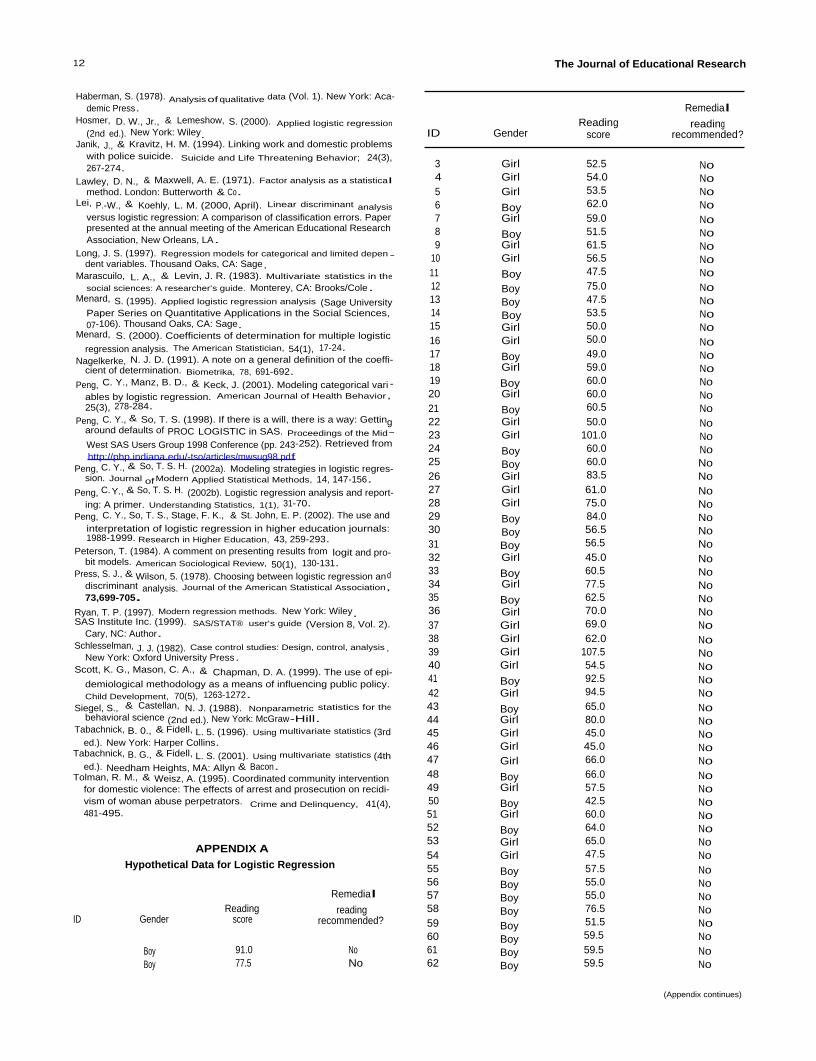
APPENDIX A

Hypothetical Data for Logistic Regression

RemedialReading reading

ID Gender score recommended?

Boy 91.0 NoBoy 77.5 No

The Journal of Educational Research

ID GenderReading

score

Remedial

readingrecommended?

3 Girl 52.5 No4 Girl 54.0 No5 Girl 53.5 No6 Boy 62.0 No7 Girl 59.0 No8 Boy 51.5 No9 Girl 61.5 No

10 Girl 56.5 No11 Boy 47.5 No12 Boy 75.0 No13 Boy 47.5 No14 Boy 53.5 No15 Girl 50.0 No16 Girl 50.0 No17 Boy 49.0 No18 Girl 59.0 No19 Boy 60.0 No20 Girl 60.0 No21 Boy 60.5 No22 Girl 50.0 No23 Girl 101.0 No24 Boy 60.0 No25 Boy 60.0 No26 Girl 83.5 No27 Girl 61.0 No28 Girl 75.0 No29 Boy 84.0 No30 Boy 56.5 No31 Boy 56.5 No32 Girl 45.0 No33 Boy 60.5 No34 Girl 77.5 No35 Boy 62.5 No36 Girl 70.0 No37 Girl 69.0 No38 Girl 62.0 No39 Girl 107.5 No40 Girl 54.5 No41 Boy 92.5 No42 Girl 94.5 No43 Boy 65.0 No44 Girl 80.0 No45 Girl 45.0 No46 Girl 45.0 No47 Girl 66.0 No48 Boy 66.0 No49 Girl 57.5 No50 Boy 42.5 No51 Girl 60.0 No52 Boy 64.0 No53 Girl 65.0 No54 Girl 47.5 No55 Boy 57.5 No56 Boy 55.0 No57 Boy 55.0 No58 Boy 76.5 No59 Boy 51.5 No60 Boy 59.5 No61 Boy 59.5 No62 Boy 59.5 No

(Appendix continues)

September/October 2002 [Vol. 96(No. 1)] 13

APPENDIX A-continued

Remedial RemedialReading reading Reading reading

ID Gender score recommended? ID Gender score recommended?

63 Boy 55.0 No 122 Boy 80.0 No64 Girl 70.0 No 123 Girl 57.5 No65 Boy 66.5 No 124 Girl 64.5 No66 Boy 84.5 No 125 Girl 65.0 No67 Boy 57.5 No 126 Girl 60.0 No68 Boy 125.0 No 127 Girl 85.0 No69 Girl 70.5 No 128 Girl 60.0 No70 Boy 79.0 No 129 Girl 58.0 No71 Girl 56.0 No 130 Girl 61.5 No72 Boy 75.0 No 131 Boy 60.0 Yes73 Boy 57.5 No 132 Girl 65.0 Yes74 Boy 56.0 No 133 Boy 93.5 Yes75 Girl 67.5 No 134 Boy 52.5 Yes76 Boy 114.5 No 135 Boy 42.5 Yes77 Girl 70.0 No 136 Boy 75.0 Yes78 Girl 67.0 No 137 Boy 48.5 Yes79 Boy 60.5 No 138 Boy 64.0 Yes80 Girl 95.0 No 139 Boy 66.0 Yes81 Girl 65.5 No 140 Girl 82.5 Yes82 Girl 85.0 No 141 Girl 52.5 Yes83 Boy 55.0 No 142 Girl 45.5 Yes84 Boy 63.5 No 143 Boy 57.5 Yes85 Boy 61.5 No 144 Boy 65.0 Yes86 Boy 60.0 No 145 Girl 46.0 Yes87 Boy 52.5 No 146 Girl 75.0 Yes88 Girl 65.0 No 147 Boy 100.0 Yes89 Girl 87.5 No 148 Girl 77.5 Yes90 Girl 62.5 No 149 Boy 51.5 Yes91 Girl 66.5 No 150 Boy 62.5 Yes92 Boy 67.0 No 151 Boy 44.5 Yes93 Girl 117.5 No 152 Girl 51.0 Yes94 Girl 47.5 No 153 Girl 56.0 Yes95 Girl 67.5 No 154 Girl 58.5 Yes96 Girl 67.5 No 155 Girl 69.0 Yes97 Girl 77.0 No 156 Boy 65.0 Yes98 Girl 73.5 No 157 Boy 60.0 Yes99 Girl 73.5 No 158 Girl 65.0 Yes

100 Girl 68.5 No 159 Boy 65.0 Yes101 Girl 55.0 No 160 Boy 40.0 Yes102 Girl 92.0 No 161 Girl 55.0 Yes103 Boy 55.0 No 162 Boy 52.5 Yes104 Girl 55.0 No 163 Boy 54.5 Yes105 Boy 60.0 No 164 Boy 74.0 Yes106 Boy 120.5 No 165 Boy 55.0 Yes107 Girl 56.0 No 166 Girl 60.5 Yes108 Girl 84.5 No 167 Boy 50.0 Yes109 Girl 60.0 No 168 Boy 48.0 Yes110 Boy 85.0 No 169 Girl 51.0 Yes111 Girl 93.0 No 170 Girl 55.0 Yes112 Boy 60.0 No 171 Boy 93.5 Yes113 Girl 65.0 No 172 Boy 61.0 Yes114 Girl 58.5 No 173 Boy 52.5 Yes115 Girl 85.0 No 174 Boy 57.5 Yes116 Boy 67.0 No 175 Boy 60.0 Yes117 Girl 67.5 No 176 Girl 71.0 Yes118 Boy 65.0 No 177 Girl 65.0 Yes119 Girl 60.0 No 178 Girl 60.0 Yes120 Boy 47.5 No 179 Girl 55.0 Yes121 Girl 79.0 No 180 Boy 60.0 Yes

(Appendix continues)

14

APPENDIX A-continued

ID GenderReading

score

Remedialreading

recommended?

181 Boy 77.0 Yes182 Boy 52.5 Yes183 Girl 95.0 Yes184 Boy 50.0 Yes185 Girl 47.5 Yes186 Boy 50.0 Yes187 Boy 47.0 Yes188 Boy 71.0 Yes189 Girl 65.0 Yes

APPENDIX BList of JER Articles Reviewed

1. Alexander, K. L., Dauber, S. L., & Entwisle, D. R. (1996).Children in motion: School transfers and elementary school per-formance. The Journal of Educational Research, 90(1), 3-11.

2. Diamond, K. E., Reagan, A J., & Bandyk, J. E. (2000). Par-

ents' conceptions of kindergarten readiness: Relationships withrace, ethnicity, and development. The Journal of EducationalResearch, 94(2), 93-100.

3. Machamer, A. M., & Gruber, E. (1998). Secondary school,family, and educational risk: Comparing American Indian adoles-cents and their peers. The Journal of Educational Research, 91(6),357-369.

4. McNeal, R. B., Jr. (1998). High school extracurricular activi-ties: Closed structures and stratifying patterns of participation.The Journal of Educational Research, 91(3), 183-191.

5. Meisels, S. J., & Liaw, F.-R. (1993). Failure in grade: Doretained students catch up? The Journal of Educational Research,

87(2), 69-77.

6. Rush, S., & Vitale, P. A. (1994). Analysis for determining fac-tors that place elementary students at risk. The Journal of Educa-tional Research, 87(6), 325-333.

7. Smith, J. B. (1997). Effects of eighth-grade transition pro-grams on high school retention and experiences. The Journal ofEducational Research, 90(3), 144-152.

8. Trusty, J. (2000). High educational expectations and lowachievement: Stability of educational goals across adolescence.The Journal of Educational Research, 93(6), 356-365.

Advertise inThe Journal of Educational Research

For more information please contact :

Alison Mayhew, Advertising ManagerHeldref Publications

1319 Eighteenth St NW

Washington. DC 20036-1802

Phone: (202) 296-6267 Fax: (202) 293-6130

The Journal of Educational Research

4k,

32,000,000 Americans

wish they weren't here.It's a state so vast you can travel from the

Atlantic to the Pacific and never leave it behind.

So enormous that it touches one out of every

eleven families in America. So huge that it

embraces one out of every six children in

America - and holds them in its cruel grip. And

with a population of 32 million, it's the second

largest state in the nation. It's the state of poverty

in America. And though many people live here,

it doesn't feel like home.

POVERTY.Americas forgotten state.

Catholic Campaign for Human Development

1-800-946-4243

www.povertyusa.org0J