An Introduction to Implied Levy Volatility with Applications ∗∗∗

Marc Cassagnol†

August 30, 2010

Abstract

The concept of implied volatility is one of the great successes of the Black-Scholes model.However, Black-Scholes relies on a normal distribution, which historical data shows is notadequate to describe real markets. This is often seen in implied volatility surfaces which“smile” and “smirk”, taking on different values for different strike prices. In this paper wediscuss a more empirically founded type of implied volatility based on Levy distributions,first introduced by Corcuera, Guillaume, Leoni and Schoutens in 2009. We use implied Levyvolatility with real market prices to reduce the presence of smiles and smirks. We performseveral delta and gamma hedging experiments to test the performance of the Black-Scholesmodel against Levy models. Finally, we price barrier options using implied Black-Scholes andimplied Levy volatility and discuss how the change in volatility affects the prices.

∗Department of Mathematics and Statistics, York University. Submitted in partial fulfillmentof requirements of Master of Arts in Mathematics and Statistics, under the supervision of Prof. HannaJankowski.∗∗Schulich School of Business, York University. Submitted in partial fulfillment of requirements

of Graduate Diploma in Financial Engineering.†Email address: mjgc@mathstat.yorku.ca

1

Contents

1 Introduction 3

2 Fundamental concepts 42.1 The Black-Scholes model . . . . . . . . . . . . . . . . . . . . . . . . . . . . . 42.2 Implied volatility . . . . . . . . . . . . . . . . . . . . . . . . . . . . . . . . . 52.3 Hedging with the Greeks . . . . . . . . . . . . . . . . . . . . . . . . . . . . . 52.4 Barrier options . . . . . . . . . . . . . . . . . . . . . . . . . . . . . . . . . . 7

3 Levy framework 83.1 Shortcomings of the Black-Scholes model . . . . . . . . . . . . . . . . . . . . 83.2 Levy processes . . . . . . . . . . . . . . . . . . . . . . . . . . . . . . . . . . 93.3 Calculating option prices and Greeks under Levy models . . . . . . . . . . . 11

3.3.1 Call option pricing using characteristic functions . . . . . . . . . . . 113.3.2 Calculation of delta . . . . . . . . . . . . . . . . . . . . . . . . . . . 123.3.3 Calculation of gamma . . . . . . . . . . . . . . . . . . . . . . . . . . 12

3.4 Simulating Levy processes . . . . . . . . . . . . . . . . . . . . . . . . . . . . 13

4 Implied Levy volatility 144.1 Implied Levy space volatility . . . . . . . . . . . . . . . . . . . . . . . . . . 144.2 Implied Levy time volatility . . . . . . . . . . . . . . . . . . . . . . . . . . . 154.3 Black-Scholes smiles and Levy waves . . . . . . . . . . . . . . . . . . . . . . 164.4 Black-Scholes smirks and Levy waves . . . . . . . . . . . . . . . . . . . . . . 17

5 Hedging performance 185.1 Delta hedging . . . . . . . . . . . . . . . . . . . . . . . . . . . . . . . . . . . 195.2 Gamma hedging . . . . . . . . . . . . . . . . . . . . . . . . . . . . . . . . . 215.3 Delta and gamma hedging . . . . . . . . . . . . . . . . . . . . . . . . . . . . 22

6 Barrier pricing performance 246.1 Geometric Brownian motion price process . . . . . . . . . . . . . . . . . . . 246.2 Levy price process . . . . . . . . . . . . . . . . . . . . . . . . . . . . . . . . 25

7 Conclusion 26

8 Future Work 27

2

1 Introduction

The Black-Scholes model has seen paramount success partially due to the concept of impliedvolatility which it introduced. Implied volatility allows traders to match market prices withtheoretical model prices in a consistent way. It is often convenient to quote vanilla optionsby their implied Black-Scholes volatility as it does not require units of currency, and tradershave gained an intuition for this quantity over the years. Implied volatility depends on strikeprice and time to maturity, and so it is usually reported as a curve or surface.

The drawback of implementing implied volatility using the Black-Scholes pricing modelis that it is based on a normal distribution. Historical data indicates that return distribu-tions on stocks are often skewed and heavier-tailed than can be described by the normaldistribution. As a result of this, when implied Black-Scholes volatility is calculated for realoption prices, the surfaces often “smile” or “smirk” with respect to strike price. The factthat different strikes yield different values for implied volatility indicates that the modeldoes not accurately describe the behaviour of the stock. This creates a problem when pric-ing barrier options concerning which volatility to use as input; the volatility correspondingto the strike price, the barrier level, or perhaps some average of these two values.

In this paper we discuss Levy distributions and the additional freedom they providein calibrating skewness and kurtosis. We discuss a more generalized version of impliedvolatility which works for Levy processes. Since Brownian motion is itself a Levy process,the models discussed here reduce to the Black-Scholes model if a Brownian motion is used.The concept of implied Levy volatility was first introduced in 2009 by Corcuera, Guillaume,Leoni and Schoutens in [6]. They discussed implied Levy space and time volatility models,both of which will be covered here in great detail.

In addition, we discuss the Carr-Madan approach to option pricing using the fast Fouriertransform (FFT). This method can be implemented for any Levy process whose charac-teristic function is computable. This formulation will be used for implied Levy volatilitycalculations. We also use the Carr-Madan formula to derive the delta and gamma of a calloption under the Levy framework. This will allow us to perform hedging experiments usingLevy models.

One of the benefits of using implied Levy volatility is that the additional degrees offreedom provided by the model can be used to reduce the presence of smiling in the impliedvolatility surface. In Section 4 we examine options on AAPL stock that exhibit both smilingand smirking implied Black-Scholes volatility. We calibrate the corresponding implied Levyspace and time volatility models to yield flatter curves, suggesting that Levy models arecapable of more accurately describe the stock price.

In Section 5 we compare the performance of delta and gamma hedges when Black-Scholes and Levy parameters are used. Using data which covers the 2007 financial crisis,we hedge a rolling at-the-money option on the S&P 500 and investigate the performanceof the hedges under various models. Evaluating the hedging performance during the crisisworks as a stress test for the models. We determine the optimal parameter settings whichlead to the smallest hedging error for each model.

In Section 6 we price barrier options using Monte Carlo simulation and the impliedBlack-Scholes and Levy volatility data from Section 4. We investigate how the flattervolatility curve affects the range of barrier option prices using both geometric Brownian

3

motion and a normal inverse Gaussian process to drive the simulations. We discuss severalways that volatility can directly or indirectly affect the price of barrier options. Finallywe formulate our conclusions in Section 7 and discuss some areas where this work can beexpanded upon in the future in Section 8.

2 Fundamental concepts

2.1 The Black-Scholes model

The Black-Scholes model assumes that the risk-neutral price process for the underlyingstock follows a geometric Brownian motion:

St = S0 e(r−q−σ2/2)t+σWt

where t ≥ 0, is the time remaining until maturity, r ≥ 0 is the risk-free interest rate, q ≥ 0is the dividend yield, σ > 0 is the volatility parameter and Wt is a standard Brownianmotion. To verify that this is a risk-neutral process, we must show that

E[St|Fτ ] = St e(r−q)(t−τ)

for any t > τ . We do this by showing that Xt = S0 eσWt−σ2t/2 is a martingale:

dXt =∂X

∂tXt dt+

∂X

∂wXt dWt +

1

2

∂2X

∂w2Xt (dWt)

2

= −1

2σ2Xt dt+ σXt dWt +

1

2σ2Xt(dt)

= σXt dWt.

This shows that the drift of the process St = Xt e(r−q)t is equal to (r − q) dt which implies

that the expected continuous log-return of the stock is the risk-free rate (minus the dividendyield). Equipped with this model, one can calculate the price of a vanilla European calloption to be the famous Black-Scholes formula:

C(S0,K, T, r, σ, q) = S0 e−qTN(d1)−K e−rTN(d2) (1)

where

d1 =log(S0/K) + (r − q + σ2/2)T

σ√T

,

d2 = d1 − σ√T ,

and N(·) is the standard normal cumulative distribution function. At any given time, theparameters S0, r, σ and q are the same for every derivative written on the asset, so whenpricing options it is convenient to abbreviate the call price function as C(K,T ) which wewill do whenever possible.

4

2.2 Implied volatility

After the introduction of the Black-Scholes model during the 1970’s, traders began usingit to calibrate their models. Rather than calculating volatility by tracking the stock price,calculating daily returns and computing the standard deviation of the return distribution,they would find the value for volatility σ(K,T ) such that when plugged into the Black-Scholes formula, the resulting price equalled the current market price. This value is calledthe implied Black-Scholes volatility, or simply the implied volatility of the option, and itrepresents what volatility the market deems appropriate for the stock.

220 240 260 280 300 320 340 360 3800.25

0.3

0.35

0.4

0.45

0.5Implied Black−Scholes Volatilities of AAPL Calls (27 July 2010)

K

σ

AUG 10SEP 10OCT 10JAN 11JAN 12

Figure 1: Implied Black-Scholes volatility for sev-eral AAPL calls; S0 = 264.08. Data Source: Yahoo!Finance, July 27, 2010.

When the Black-Scholes model is usedto calculate implied volatility one often ob-tains different numbers for different valuesof K and T . In particular, a “smile” or“smirk” shape is often observed in the plotof implied volatility versus strike price. Im-plied volatility tends to increase with ma-turity time, but is often larger for optionswith very short maturities. This is due tothe increase in price that sometimes occurswhen options are close to maturity as theprice and the payoff converge.

2.3 Hedging with the Greeks

The Greeks of an option measure the sen-sitivity of its price with respect to its in-put parameters S0,K, T, r and σ. Knowingthese sensitivities helps traders to hedge more effectively. The most common way to hedgea portfolio is to make it insensitive to changes in the underlying stock. The relevant Greeksfor this are the first and second derivatives of the option price with respect to spot price;delta (∆) and gamma (Γ) respectively. By differentiating the Black-Scholes formula withrespect to S0 we obtain the Black-Scholes delta:

∆ =∂C

∂S0

=∂

∂S0

[S0 e

−qTN(d1)−K e−rTN(d2)]

= e−qTN(d1) + S0 e−qT ∂N(d1)

∂S0−K e−rT

∂N(d2)

∂S0

= e−qTN(d1) + S0 e−qT 1

S0 σ√Tn(d1)−K e−rT

1

S0 σ√Tn(d2)

= e−qTN(d1) +1

S0 σ√T

[S0 e

−qT n(d1)−K e−rT n(d2)]

= e−qTN(d1)

5

where n(·) is the standard normal probability density function. We have used the identityS0 e

−qT n(d1) = K e−rT n(d2) in the last line. We differentiate delta with respect to S0 toobtain gamma:

Γ = e−qT∂

∂S0N(d!)

= e−qT n(d1)∂d1∂S0

= e−qTn(d1)

S0 σ√T.

The ability to create a perfect continuous delta hedge is the basis for the arbitrageargument which gives rise to the Black-Scholes formula. A perfectly hedged portfolio canbe created by holding a long call option and −∆ shares of the underlying asset or the reverseposition; a short call option and ∆ shares of the underlying. The purpose of holding theunderlying is to neutralize the instantaneous sensitivity of the portfolio with respect tothe spot price; the delta of the portfolio is simply the sum of the deltas of the option andunderlying:

∆portfolio = ±∆call ∓∆call∂S0∂S0

= 0, (2)

and so we call such a portfolio delta neutral. To maintain a perfect hedge, the portfolio mustbe rebalanced continuously, as the delta of the option changes due to movements in thestock price and and the passage of time. Therefore it is practically impossible to implementthis strategy, as there will always be a measurable period of time between trades. The riskthat arises by trading in discrete time is a form of gap risk ; which is the risk associatedwith the value of the underlying changing in between trades.

An obvious way to manage gap risk is to rebalance more often. However, in practice thiscan get expensive due to the transaction costs associated with trading. A better approachis to further reduce the sensitivity of the portfolio in order to marginalize the change invalue that could occur between trades. This can be achieved through gamma hedging. Aportfolio is gamma neutral if the second derivative of its value with respect to the spotprice equals zero. If the delta of the portfolio truly did not change over an interval of time,there would be no need to rebalance continuously, and this gamma hedge would have zerohedging error. However this is not always the case and thus one can not guarantee thata discretely rebalanced delta/gamma hedge will always outperform a discretely rebalanceddelta hedge.

Purchasing the underlying asset has no effect on the gamma of the portfolio, as it hasa gamma value of zero. So in order to neutralize the gamma of an option, one must useanother derivative security written on the same underlying asset. Usually another optionwith a different strike price is used. Since this option will be sold and repurchased onoccasion, one would in practice want to use a liquid option for this purpose, such as anoption which is close to being at-the-money.

Let ∆ and Γ denote the delta and gamma of the option we want to hedge, and ∆′

and Γ′ denote the delta and gamma of the option we are using to create the hedge. Leta denote the amount of underlying necessary to neutralize the delta of the options in the

6

portfolio, and b denote the amount of the second option we need to purchase to neutralizethe gamma. To obtain a zero portfolio delta we then need

∆ + a+ b∆′ = 0. (3)

To obtain a zero portfolio gamma we need

Γ + bΓ′ = 0. (4)

Equation (4) shows that we must hold the opposite position

b = − Γ

Γ′

in the second option to neutralize the gamma of the first option. Therefore in order todelta-hedge the portfolio we must hold

a = −∆ +Γ

Γ′∆′

units of the underlying stock.In addition to hedging away the delta and gamma of the portfolio, it will be convenient

for us to also maintain a portfolio with zero value. This can be achieved by taking a positionin the money market (either borrowing or lending) equal to minus the value of the stocksand options in the portfolio. The benefit of constructing the portfolio this way is that thehedging error is simply equal to the portfolio value, with a perfect hedge having a portfoliovalue of zero. This makes is straight forward to calculate a hedging error distribution toevaluate the performance of the hedge.

As an example of how hedging error is calculated, consider the following delta hedgecalculation. Beginning with a brand new call with price C(K,T ) and delta ∆ we delta-hedgethis option by purchasing −∆ shares of the underlying asset. The value of the portfolio isnow

V0 = C(K,T )−∆S0.

In addition to this, we invest−(C(K,T )−∆S0)

in the money market which makes the value of the portfolio equal to zero. The next day(after δt time has passed) the value of the portfolio is:

Vδt = C(K,T − δt)−∆Sδt − (C(K,T )−∆S0)erδt.

If our hedge was perfect, we would have Vδt = 0. Hence the hedging error (any deviationfrom zero) can be measured by the value of Vδt.

2.4 Barrier options

A barrier option is an exotic option which pays depending on whether or not the underlyingstock price reaches a predetermined price called the barrier level, denoted by B, at sometime before maturity. We will look at four varieties of barrier options:

7

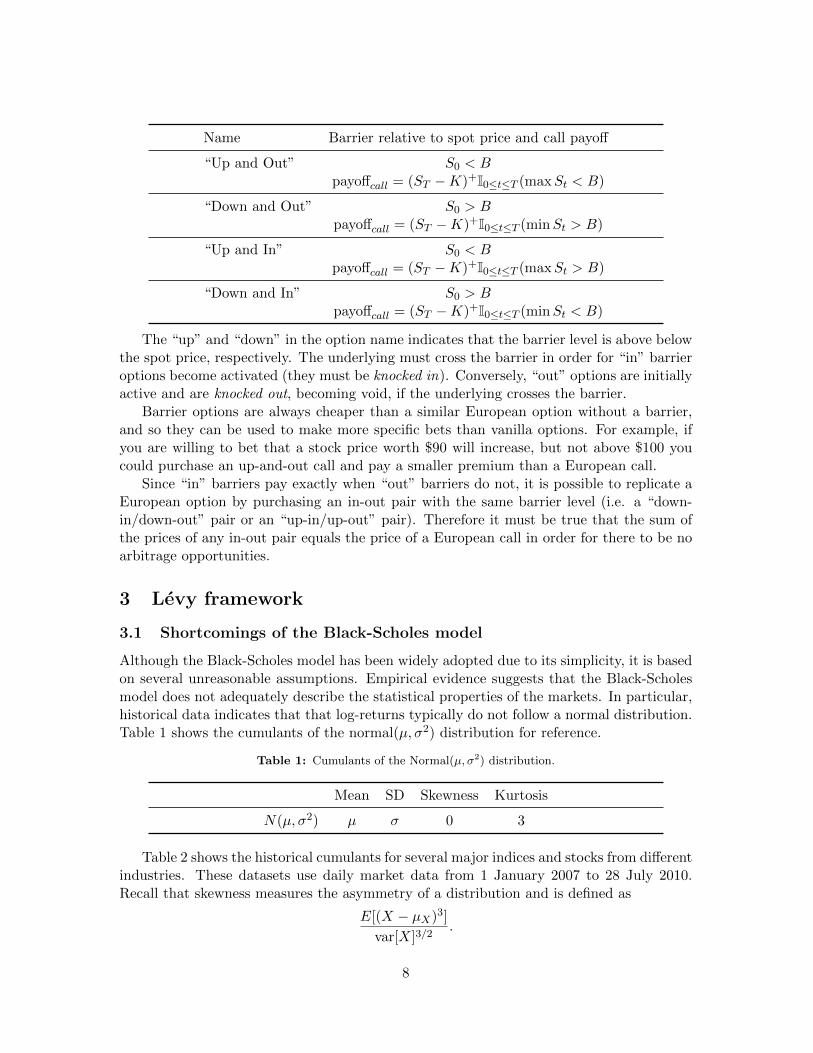
Name Barrier relative to spot price and call payoff

“Up and Out” S0 < Bpayoffcall = (ST −K)+I0≤t≤T (maxSt < B)

“Down and Out” S0 > Bpayoffcall = (ST −K)+I0≤t≤T (minSt > B)

“Up and In” S0 < Bpayoffcall = (ST −K)+I0≤t≤T (maxSt > B)

“Down and In” S0 > Bpayoffcall = (ST −K)+I0≤t≤T (minSt < B)

The “up” and “down” in the option name indicates that the barrier level is above belowthe spot price, respectively. The underlying must cross the barrier in order for “in” barrieroptions become activated (they must be knocked in). Conversely, “out” options are initiallyactive and are knocked out, becoming void, if the underlying crosses the barrier.

Barrier options are always cheaper than a similar European option without a barrier,and so they can be used to make more specific bets than vanilla options. For example, ifyou are willing to bet that a stock price worth $90 will increase, but not above $100 youcould purchase an up-and-out call and pay a smaller premium than a European call.

Since “in” barriers pay exactly when “out” barriers do not, it is possible to replicate aEuropean option by purchasing an in-out pair with the same barrier level (i.e. a “down-in/down-out” pair or an “up-in/up-out” pair). Therefore it must be true that the sum ofthe prices of any in-out pair equals the price of a European call in order for there to be noarbitrage opportunities.

3 Levy framework

3.1 Shortcomings of the Black-Scholes model

Although the Black-Scholes model has been widely adopted due to its simplicity, it is basedon several unreasonable assumptions. Empirical evidence suggests that the Black-Scholesmodel does not adequately describe the statistical properties of the markets. In particular,historical data indicates that that log-returns typically do not follow a normal distribution.Table 1 shows the cumulants of the normal(µ, σ2) distribution for reference.

Table 1: Cumulants of the Normal(µ, σ2) distribution.

Mean SD Skewness Kurtosis

N(µ, σ2) µ σ 0 3

Table 2 shows the historical cumulants for several major indices and stocks from differentindustries. These datasets use daily market data from 1 January 2007 to 28 July 2010.Recall that skewness measures the asymmetry of a distribution and is defined as

E[(X − µX)3]

var[X]3/2.

8

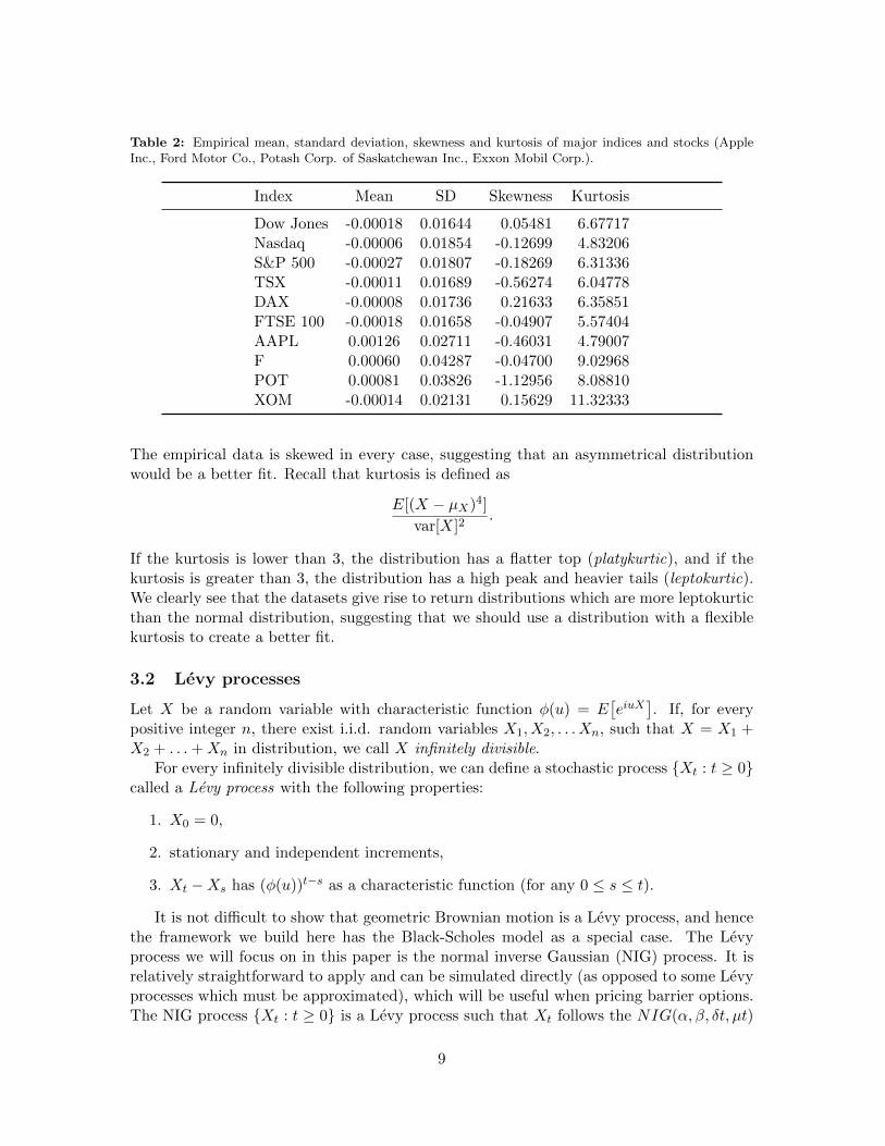
Table 2: Empirical mean, standard deviation, skewness and kurtosis of major indices and stocks (AppleInc., Ford Motor Co., Potash Corp. of Saskatchewan Inc., Exxon Mobil Corp.).

Index Mean SD Skewness Kurtosis

Dow Jones -0.00018 0.01644 0.05481 6.67717Nasdaq -0.00006 0.01854 -0.12699 4.83206S&P 500 -0.00027 0.01807 -0.18269 6.31336TSX -0.00011 0.01689 -0.56274 6.04778DAX -0.00008 0.01736 0.21633 6.35851FTSE 100 -0.00018 0.01658 -0.04907 5.57404AAPL 0.00126 0.02711 -0.46031 4.79007F 0.00060 0.04287 -0.04700 9.02968POT 0.00081 0.03826 -1.12956 8.08810XOM -0.00014 0.02131 0.15629 11.32333

The empirical data is skewed in every case, suggesting that an asymmetrical distributionwould be a better fit. Recall that kurtosis is defined as

E[(X − µX)4]

var[X]2.

If the kurtosis is lower than 3, the distribution has a flatter top (platykurtic), and if thekurtosis is greater than 3, the distribution has a high peak and heavier tails (leptokurtic).We clearly see that the datasets give rise to return distributions which are more leptokurticthan the normal distribution, suggesting that we should use a distribution with a flexiblekurtosis to create a better fit.

3.2 Levy processes

Let X be a random variable with characteristic function φ(u) = E[eiuX

]. If, for every

positive integer n, there exist i.i.d. random variables X1, X2, . . . Xn, such that X = X1 +X2 + . . .+Xn in distribution, we call X infinitely divisible.

For every infinitely divisible distribution, we can define a stochastic process {Xt : t ≥ 0}called a Levy process with the following properties:

1. X0 = 0,

2. stationary and independent increments,

3. Xt −Xs has (φ(u))t−s as a characteristic function (for any 0 ≤ s ≤ t).

It is not difficult to show that geometric Brownian motion is a Levy process, and hencethe framework we build here has the Black-Scholes model as a special case. The Levyprocess we will focus on in this paper is the normal inverse Gaussian (NIG) process. It isrelatively straightforward to apply and can be simulated directly (as opposed to some Levyprocesses which must be approximated), which will be useful when pricing barrier options.The NIG process {Xt : t ≥ 0} is a Levy process such that Xt follows the NIG(α, β, δt, µt)

9

−5 −4 −3 −2 −1 0 1 2 3 4 50

0.1

0.2

0.3

0.4

0.5

0.6

0.7

0.8

f(x)

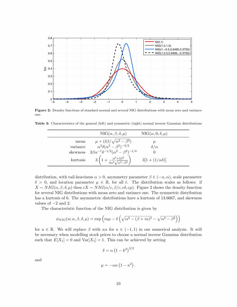
N(0,1)NIG(1,0,1,0)NIG(1,−0.5,0.6495,0.3750)NIG(1,0.5,0.6495,−0.3750)

Figure 2: Density functions of standard normal and several NIG distributions with mean zero and varianceone.

Table 3: Characteristics of the general (left) and symmetric (right) normal inverse Gaussian distributions

NIG(α, β, δ, µ) NIG(α, 0, δ, µ)

mean µ+ (δβ/√α2 − β2) µ

variance α2δ(α2 − β2)−3/2 δ/α

skewness 3βα−1δ−1/2(α2 − β2)−1/4 0

kurtosis 3

(1 + α2+4β2

δα2√α2−β2

)3[1 + (1/αδ)]

distribution, with tail-heaviness α > 0, asymmetry parameter β ∈ (−α, α), scale parameterδ > 0, and location parameter µ ∈ R, for all t. The distribution scales as follows: ifX ∼ NIG(α, β, δ, µ) then cX ∼ NIG(α/c, β/c, cδ, cµ). Figure 2 shows the density functionfor several NIG distributions with mean zero and variance one. The symmetric distributionhas a kurtosis of 6. The asymmetric distributions have a kurtosis of 13.6667, and skewnessvalues of −2 and 2.

The characteristic function of the NIG distribution is given by

φNIG(u;α, β, δ, µ) = exp(iuµ− δ

(√α2 − (β + iu)2 −

√α2 − β2

))for u ∈ R. We will replace β with κα for κ ∈ (−1, 1) in our numerical analysis. It willbe necessary when modelling stock prices to choose a normal inverse Gaussian distributionsuch that E[X1] = 0 and Var[X1] = 1. This can be achieved by setting

δ = α(1− k2

)3/2and

µ = −ακ(1− κ2

).

10

3.3 Calculating option prices and Greeks under Levy models

When we remove the assumption that the stock price follows a geometric Brownian motionin favour of a more general semi-martingale (of which Levy processes are a subset), thefundamental theorem of asset pricing no longer holds. In particular, we lose market com-pleteness as there is no longer a unique risk-neutral measure. This means we also lose theability to perfectly hedge an option through continuous-time delta hedging. However, sincetrading is always performed discretely in practice, the non-existence of a perfect continuoushedge will not affect our ability to hedge under Levy models. Most practitioners believethat the market is incomplete, so a pricing model which supports market incompleteness isdesirable.

3.3.1 Call option pricing using characteristic functions

Following [4], we price options as follows. Let Q denote a measure such that the discountedstock price is a martingale. The price C(K,T ) of a European call option with strike K andmaturity T can be defined as the expected price (under Q) at maturity, discounted by therisk-free rate:

C(K,T ) = e−rTEQ[(ST −K)+]. (5)

Under the Black-Scholes model, this is the unique arbitrage-free price. Under the generalLevy framework, this price lies in an interval of arbitrage-free prices corresponding to arange of martingale measures.

Whenever the risk-neutral density function is available, (5) can be evaluated analytically.However, it is usually a lengthy process. A faster approach is to use the fast Fouriertransform (FFT) method developed by Carr and Madan in [4]. Their formula for the priceof the European call option is

C(K,T ) =e−λ log(K)

π

∫ ∞0

e−iv log(K)ψT (v) dv (6)

where

ψT (v) =e−rTϕT (v − (λ+ 1)i)

(λ+ iv)(λ+ 1 + iv),

and λ > 0 is a parameter which ensures the result ψT (v) is finite. The only part of thisformulation which depends on the model is the function ϕT (u) which is (under Q) thecharacteristic function of the log-price process at maturity T ,

ϕT (u) = EQ[eiu log(ST )].

The benefit of this approach to option pricing is that it can be implemented for anyLevy distribution whose characteristic function is available analytically. This gives us thefreedom to use distributions with skewness and kurtosis which better match empirical valuesfrom the market. (6) can be evaluated numerically very quickly with the help of the inversefast Fourier transform. The formulation can be used to price put options as well, throughput-call parity.

11

3.3.2 Calculation of delta

The delta of an option is defined analogously in the Levy case; it measures the sensitivityof the option with respect to changes in the underlying stock price. To calculate delta, wedifferentiate (6):

∆ =∂

∂S0

[e−λ log(K)

π

∫ ∞0

e−iv log(K) e−rTϕT (v − (λ+ 1)i)

λ2 + λ− v2 + i(2λ+ 1)vdv

]

=e−λ log(K)

π

∫ ∞0

e−iv log(K)e−rT

λ2 + λ− v2 + i(2λ+ 1)v

∂ [ϕT (v − (λ+ 1)i)]

∂S0dv. (7)

In order to formulate this explicitly, we evaluate

∂ [ϕT (v − (λ+ 1)i)]

∂S0=

∂

∂S0EQ[ei(v−(λ+1)i) log(ST )]

=∂

∂S0EQ[ei(v−(λ+1)i)[log(S0)+log(e(r−q+ω)T+σXT )]]

= i(v − (λ+ 1)i)1

S0EQ[ei(v−(λ+1)i)[log(S0)+log(e(r−q+ω)T+σXT )]]

=λ+ 1 + vi

S0ϕT (v − (λ+ 1)i). (8)

Combining this result with equation (7), and using the fact that λ2+λ−v2+i(2λ+1)v =(λ+ vi)(λ+ 1 + vi) we obtain

∆ =e−λ log(K)

π

∫ ∞0

e−iv log(K)e−rT

(λ+ vi)(λ+ 1 + vi)

λ+ 1 + vi

S0ϕT (v − (λ+ 1)i) dv

=e−λ log(K)

π

∫ ∞0

e−iv log(K)e−rT

S0(λ+ vi)ϕT (v − (λ+ 1)i) dv. (9)

3.3.3 Calculation of gamma

The gamma of an option measures the second order sensitivity of the option with respectto the underlying stock price.

Γ =∂2C(K,T )

∂S20

=∂∆

∂S0.

We calculate gamma using the results of (8) and (9):

12

Γ =∂

∂S0

[e−λ log(K)

π

∫ ∞0

e−iv log(K)e−rT

S0(λ+ vi)ϕT (v − (λ+ 1)i) dv

]

=e−λ log(K)

π

∫ ∞0

e−iv log(K)e−rT

(λ+ vi)

∂

∂S0

[ϕT (v − (λ+ 1)i)

S0

]dv

=e−λ log(K)

π

∫ ∞0

e−iv log(K)e−rT

(λ+ vi)

[λ+1+viS0

ϕT (v − (λ+ 1)i)(S0)− (1)ϕT (v − (λ+ 1)i)

S20

]dv

=e−λ log(K)

π

∫ ∞0

e−iv log(K)e−rT

(λ+ vi)

[ϕT (v − (λ+ 1)i)(λ+ 1 + vi− 1)

S20

]dv

=e−λ log(K)

π

∫ ∞0

e−iv log(K)e−rT

S20

ϕT (v − (λ+ 1)i) dv. (10)

3.4 Simulating Levy processes

If one wants to perform Monte Carlo calculations using Levy processes, it is necessary tosimulate from Levy distributions. It is possible to simulate any Levy process using anapproximation of a compound Poisson process, but for specific Levy processes, there aremore sophisticated methods available. In particular, we focus on the NIG model, which canbe simulated explicitly as a time-changed Brownian motion, with random time step sizesfollowing an inverse Gaussian (IG) process. When used for option pricing, the locationparameter µ of the NIG process has no effect on the price of the option, so for conveniencewe take µ = 0.

The following algorithm can be used to simulate a sample path from a NIG(α, β, δ, 0)distribution. In order to properly simulate the stock price, the NIG process must have amean of zero and a variance of 1. Let T denote the time to maturity and Nt denote thenumber of time steps:

i. Set dt = T/Nt

ii. Set a = dt

iii. Set b = δ√α2 − β2

iv. Generate Nt standard normal random variables v1, . . . , vNt

v. Set yi = v2i for i = 1, . . . , Nt

vi. Set xi =a

b+

yi2b2−

√4abyi + y2i

2b2for i = 1, . . . , Nt

vii. Generate Nt standard uniform random variables u1, . . . , uNt

viii. If ui ≤a

a+ bxi, set ∆IGi = xi; Otherwise, set ∆IGi =

a2

xib2for i = 1, . . . , Nt

ix. Generate Nt standard normal random variables n1, . . . , nNt

13

x. Set Xi =

i∑j=1

βδ2∆IGj + δnj√

∆IGj for i = 1, . . . , Nt

The Xi values follow the desired NIG process.

4 Implied Levy volatility

We now discuss two Levy models for a stock price process which, coupled with our optionpricing model for Levy processes, gives us the necessary tools to formulate the concept ofimplied Levy volatility as introduced in [6]. We discuss Levy space and time models, bothof which can better match the heavy tails and skewness of log returns observed in Table 2.

4.1 Implied Levy space volatility

Let {Xt : t ≥ 0} be a Levy process. We denote the characteristic function of X1 by

φ1(u) = E[exp(iuX1)] .

We additionally require that E[Xt] = 0 and Var[Xt] = t, which ensures that Var[σXt] = σ2t.Under the Levy space model, the stock price process is modelled as

St = S0 e(r−q+ω)t+σXt , t ≥ 0,

whereω = − log(φ1(−σi))

is the mean correcting term necessary to make the model risk-neutral, by making thediscounted stock price a martingale. We now verify this fact.

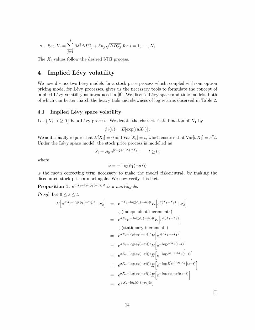
Proposition 1. eσXt−log(φ1(−σi))t is a martingale.

Proof. Let 0 ≤ s ≤ t.

E[eσXt−log(φ1(−σi))t | Fs

]= eσXs−log(φ1(−σi))tE

[eσ(Xt−Xs) | Fs

]↓ (independent increments)

= eσXse− log(φ1(−σi))tE[eσ(Xt−Xs)

]↓ (stationary increments)

= eσXs−log(φ1(−σi))tE[eσ(tX1−sX1)

]= eσXs−log(φ1(−σi))tE

[e− log eσX1 (s−t)

]= eσXs−log(φ1(−σi))tE

[e− log ei(−σi)X1 (s−t)

]= eσXs−log(φ1(−σi))tE

[e− logE[ei(−σi)X1 ](s−t)

]= eσXs−log(φ1(−σi))tE

[e− log φ1(−σi)(s−t)

]= eσXs−log(φ1(−σi))s.

14

In order to price options using the Carr-Madan formulation, we need to compute thecharacteristic function of log(ST ):

ϕT (u) = E[eiu logST

]= E

[eiu(logS0+(r−q+ω)t+σXT )

]= eiu(logS0+(r−q+ω)t)E

[eiuσXT

]= eiu(logS0+(r−q+ω)t)φT (σu).

The volatility parameter σ necessary to match the model price with a given marketprice is called the implied Levy space volatility of the option.

4.2 Implied Levy time volatility

We again begin with a Levy process {Xt : t ≥ 0} such that E[Xt] = 0 and Var[Xt] = t,and hence Var[Xσ2t] = σ2t. We denote the characteristic function of X1 by φ1(u) =E[exp(iuX1)].

St = S0 e(r−q+ωσ2)t+Xσ2t , t ≥ 0,

whereω = − log(φ1(−i))

is the mean correcting term necessary to make this new model risk-neutral. We now verifythis fact with an expectation calculation similar to the previous section.

Proposition 2. eXσ2t−log(φ1(−i))σ2t is a martingale.

Proof. Let 0 ≤ s ≤ t.

E[eXσ2t−log(φ1(−i))σ

2t | Fs]

= eXσ2s−log(φ1(−i))σ2tE[e(Xσ2t−Xσ2s) | Fs

]↓ (independent increments)

= eXσ2s− log(φ1(−i))σ2tE[e(Xσ2t−Xσ2s)

]↓ (stationary increments)

= eXσ2s− log(φ1(−i))σ2tE[e(σ

2tX1−σ2sX1)]

= eXσ2s− log(φ1(−i))σ2tE[e− log eX1 (σ2s−σ2t)

]= eXσ2s− log(φ1(−i))σ2tE

[e− log ei(−iX1)(σ2s−σ2t)

]= eXσ2s− log(φ1(−i))σ2tE

[e− logE[ei(−iX1)](σ2s−σ2t)

]= eXσ2s− log(φ1(−i))σ2tE

[e− log φ1(−i)(σ2s−σ2t)

]= eXσ2s−log(φ1(−i))σ

2s.

15

In order to price options using the Carr-Madan formulation, we need to compute thecharacteristic function of log(ST ) under this model as well:

ϕT (u) = E[eiu logST

]= E

[eiu(logS0+(r−q+ωσ2)t+Xσ2T )

]= eiu(logS0+(r−q+ωσ2)t)E

[eiuXσ2T

]= eiu(logS0+(r−q+ωσ2)t)φσ2T (u).

Similar to the Black-Scholes model, we call the volatility parameter σ necessary tomatch the model price with a given market price the implied Levy time volatility of theoption.

Notice that if we use a Brownian motion as our Levy process, then σWt and Wσ2t followthe same N(0, σ2t) distribution. Thus the space and time models coincide in the Black-Scholes setting and will yield the same option prices and implied volatilities. However thisis not always the case for more general Levy processes. Examples where the two modelsdiffer will be seen in the sections which follow.

4.3 Black-Scholes smiles and Levy waves

In this section we calculate implied Levy volatility curves for some options whose impliedBlack-Scholes volatility curve has a smile shape. We will consider how both symmetric andasymmetric NIG models perform at reducing the smile. For the data exhibiting the smileshape, we used the 27 July 2010 closing market prices of several AAPL (Apple Inc.) AUG10 calls (maturing on 20 August 2010) with the following parameter settings:

S0 = 264.08, r = 2%, q = 0, T = 24/365, K = 230, 240, . . . , 360, 370.

200 250 300 350 400

0.2

0.25

0.3

0.35

0.4

0.45

0.5

K

σ

Space σNIG(κ = 0) of AAPL AUG 10 Calls

200 250 300 350 4000.15

0.2

0.25

0.3

0.35

0.4

0.45

0.5

K

σ

Time σNIG (κ = 0) of AAPL AUG 10 Calls

BSα = 3.5α = 4α = 4.5α = 5α = 5.5

BSα = 12α = 13α = 14α = 15α = 16

Figure 3: Implied volatility for the symmetric NIG space (left) and time (right) models.

Figure 3 shows the symmetric NIG implied Levy space and time volatility curves for therange of values of α which performed the best. As we increase α, the shape of the implied

16

200 250 300 350 4000.2

0.25

0.3

0.35

0.4

0.45

0.5

K

σSpace σNIG(κ = −0.2) of AAPL AUG 10 Calls

200 250 300 350 4000.2

0.25

0.3

0.35

0.4

0.45

0.5

K

σ

Time σNIG (κ = −0.25) of AAPL AUG 10 Calls

BSα = 3.5α = 4α = 4.5α = 5α = 5.5

BSα = 12α = 13α = 14α = 15α = 16

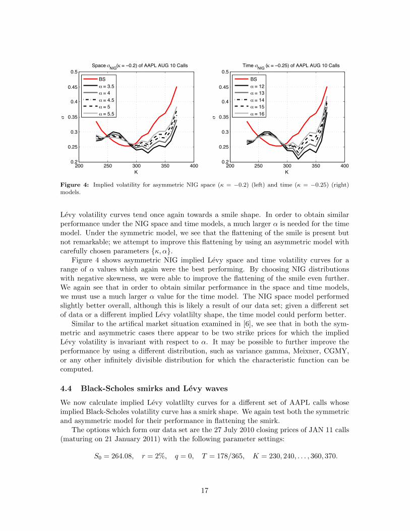
Figure 4: Implied volatility for asymmetric NIG space (κ = −0.2) (left) and time (κ = −0.25) (right)models.

Levy volatility curves tend once again towards a smile shape. In order to obtain similarperformance under the NIG space and time models, a much larger α is needed for the timemodel. Under the symmetric model, we see that the flattening of the smile is present butnot remarkable; we attempt to improve this flattening by using an asymmetric model withcarefully chosen parameters {κ, α}.

Figure 4 shows asymmetric NIG implied Levy space and time volatility curves for arange of α values which again were the best performing. By choosing NIG distributionswith negative skewness, we were able to improve the flattening of the smile even further.We again see that in order to obtain similar performance in the space and time models,we must use a much larger α value for the time model. The NIG space model performedslightly better overall, although this is likely a result of our data set; given a different setof data or a different implied Levy volatlilty shape, the time model could perform better.

Similar to the artifical market situation examined in [6], we see that in both the sym-metric and asymmetric cases there appear to be two strike prices for which the impliedLevy volatility is invariant with respect to α. It may be possible to further improve theperformance by using a different distribution, such as variance gamma, Meixner, CGMY,or any other infinitely divisible distribution for which the characteristic function can becomputed.

4.4 Black-Scholes smirks and Levy waves

We now calculate implied Levy volatlilty curves for a different set of AAPL calls whoseimplied Black-Scholes volatility curve has a smirk shape. We again test both the symmetricand asymmetric model for their performance in flattening the smirk.

The options which form our data set are the 27 July 2010 closing prices of JAN 11 calls(maturing on 21 January 2011) with the following parameter settings:

S0 = 264.08, r = 2%, q = 0, T = 178/365, K = 230, 240, . . . , 360, 370.

17

200 250 300 350 400

0.29

0.3

0.31

0.320.33

0.34

0.35

0.36

0.370.38

K

σSpace σNIG(κ = 0) of AAPL JAN 11 Calls

200 250 300 350 4000.26

0.28

0.3

0.32

0.34

0.36

0.38

K

σ

Time σNIG(κ = 0) of AAPL JAN 11 Calls

BSα = 2.5α = 3α = 3.5α = 4α = 4.5

BSα = 7α = 8α = 9α = 10α = 11

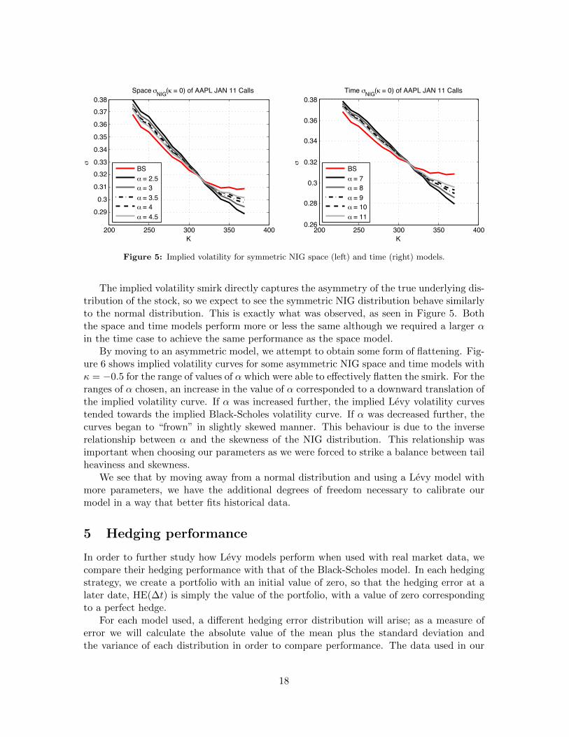
Figure 5: Implied volatility for symmetric NIG space (left) and time (right) models.

The implied volatility smirk directly captures the asymmetry of the true underlying dis-tribution of the stock, so we expect to see the symmetric NIG distribution behave similarlyto the normal distribution. This is exactly what was observed, as seen in Figure 5. Boththe space and time models perform more or less the same although we required a larger αin the time case to achieve the same performance as the space model.

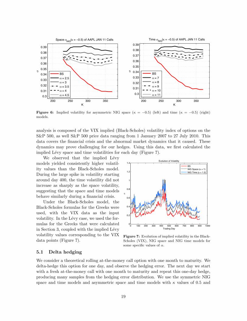
By moving to an asymmetric model, we attempt to obtain some form of flattening. Fig-ure 6 shows implied volatility curves for some asymmetric NIG space and time models withκ = −0.5 for the range of values of α which were able to effectively flatten the smirk. For theranges of α chosen, an increase in the value of α corresponded to a downward translation ofthe implied volatility curve. If α was increased further, the implied Levy volatility curvestended towards the implied Black-Scholes volatility curve. If α was decreased further, thecurves began to “frown” in slightly skewed manner. This behaviour is due to the inverserelationship between α and the skewness of the NIG distribution. This relationship wasimportant when choosing our parameters as we were forced to strike a balance between tailheaviness and skewness.

We see that by moving away from a normal distribution and using a Levy model withmore parameters, we have the additional degrees of freedom necessary to calibrate ourmodel in a way that better fits historical data.

5 Hedging performance

In order to further study how Levy models perform when used with real market data, wecompare their hedging performance with that of the Black-Scholes model. In each hedgingstrategy, we create a portfolio with an initial value of zero, so that the hedging error at alater date, HE(∆t) is simply the value of the portfolio, with a value of zero correspondingto a perfect hedge.

For each model used, a different hedging error distribution will arise; as a measure oferror we will calculate the absolute value of the mean plus the standard deviation andthe variance of each distribution in order to compare performance. The data used in our

18

200 250 300 3500.3

0.31

0.32

0.33

0.340.35

0.36

0.370.38

0.39

K

σSpace σNIG(κ = −0.5) of AAPL JAN 11 Calls

200 250 300 350

0.3

0.310.32

0.33

0.340.35

0.36

0.37

0.380.39

K

σ

Time σNIG(κ = −0.5) of AAPL JAN 11 Calls

BSα = 2.5α = 3α = 3.5α = 4α = 4.5

BSα = 7α = 8α = 9α = 10α = 11

Figure 6: Implied volatility for asymmetric NIG space (κ = −0.5) (left) and time (κ = −0.5) (right)models.

analysis is composed of the VIX implied (Black-Scholes) volatility index of options on theS&P 500, as well S&P 500 price data ranging from 1 January 2007 to 27 July 2010. Thisdata covers the financial crisis and the abnormal market dynamics that it caused. Thesedynamics may prove challenging for our hedges. Using this data, we first calculated theimplied Levy space and time volatilities for each day (Figure 7).

0 100 200 300 400 500 600 700 800 900 10000

0.2

0.4

0.6

0.8

1

1.2

1.4

Trading Day

σ

Evolution of Volatility

BSNIG Space (α = 1)NIG Time (α = 1.2)

Figure 7: Evolution of implied volatility in the Black-Scholes (VIX), NIG space and NIG time models forsome specific values of α.

We observed that the implied Levymodels yielded consistently higher volatil-ity values than the Black-Scholes model.During the large spike in volatility startingaround day 400, the time volatility did notincrease as sharply as the space volatility,suggesting that the space and time modelsbehave similarly during a financial crisis.

Under the Black-Scholes model, theBlack-Scholes formulas for the Greeks wereused, with the VIX data as the inputvolatility. In the Levy case, we used the for-mulas for the Greeks that were calculatedin Section 3, coupled with the implied Levyvolatility values corresponding to the VIXdata points (Figure 7).

5.1 Delta hedging

We consider a theoretical rolling at-the-money call option with one month to maturity. Wedelta-hedge this option for one day, and observe the hedging error. The next day we startwith a fresh at-the-money call with one month to maturity and repeat this one-day hedge,producing many samples from the hedging error distribution. We use the symmetric NIGspace and time models and asymmetric space and time models with κ values of 0.5 and

19

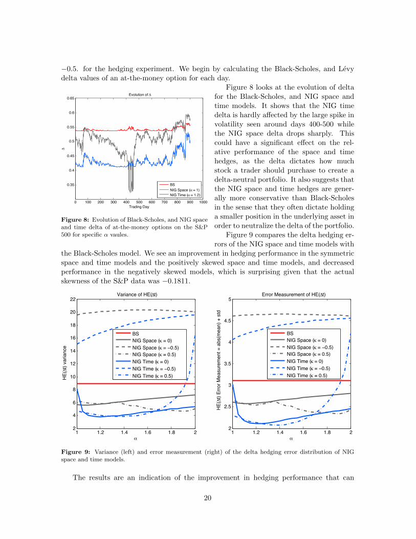
−0.5. for the hedging experiment. We begin by calculating the Black-Scholes, and Levydelta values of an at-the-money option for each day.

0 100 200 300 400 500 600 700 800 900 1000

0.35

0.4

0.45

0.5

0.55

0.6

0.65

Trading Day

Δ

Evolution of Δ

BSNIG Space (α = 1)NIG Time (α = 1.2)

Figure 8: Evolution of Black-Scholes, and NIG spaceand time delta of at-the-money options on the S&P500 for specific α vaules.

Figure 8 looks at the evolution of deltafor the Black-Scholes, and NIG space andtime models. It shows that the NIG timedelta is hardly affected by the large spike involatility seen around days 400-500 whilethe NIG space delta drops sharply. Thiscould have a significant effect on the rel-ative performance of the space and timehedges, as the delta dictates how muchstock a trader should purchase to create adelta-neutral portfolio. It also suggests thatthe NIG space and time hedges are gener-ally more conservative than Black-Scholesin the sense that they often dictate holdinga smaller position in the underlying asset inorder to neutralize the delta of the portfolio.

Figure 9 compares the delta hedging er-rors of the NIG space and time models with

the Black-Scholes model. We see an improvement in hedging performance in the symmetricspace and time models and the positively skewed space and time models, and decreasedperformance in the negatively skewed models, which is surprising given that the actualskewness of the S&P data was −0.1811.

1 1.2 1.4 1.6 1.8 22

4

6

8

10

12

14

16

18

20

22

α

HE(Δt

) var

ianc

e

Variance of HE(Δt)

1 1.2 1.4 1.6 1.8 22

2.5

3

3.5

4

4.5

5

α

HE(Δt

) Erro

r Mea

sure

men

t = a

bs(m

ean)

+ s

td

Error Measurement of HE(Δt)

BSNIG Space (κ = 0)NIG Space (κ = −0.5)NIG Space (κ = 0.5)NIG Time (κ = 0)NIG Time (κ = −0.5)NIG Time (κ = 0.5)

BSNIG Space (κ = 0)NIG Space (κ = −0.5)NIG Space (κ = 0.5)NIG Time (κ = 0)NIG Time (κ = −0.5)NIG Time (κ = 0.5)

Figure 9: Variance (left) and error measurement (right) of the delta hedging error distribution of NIGspace and time models.

The results are an indication of the improvement in hedging performance that can

20

be gained from Levy models, when given the correct parameter settings. Comparing thevariance plot with the plot of the error measurement it is clear that the standard deviationdominates the value of the error measurement.

5.2 Gamma hedging

0 200 400 600 800 10000

0.005

0.01

0.015

0.02

0.025

0.03

Trading Day

Γ

Evolution of Γ

BSNIG Space (α = 1)NIG Time (α = 1.2)

Figure 10: Evolution of Black-Scholes, and NIGspace and time gamma of at-the-money options onthe S&P 500 for specific α vaules.

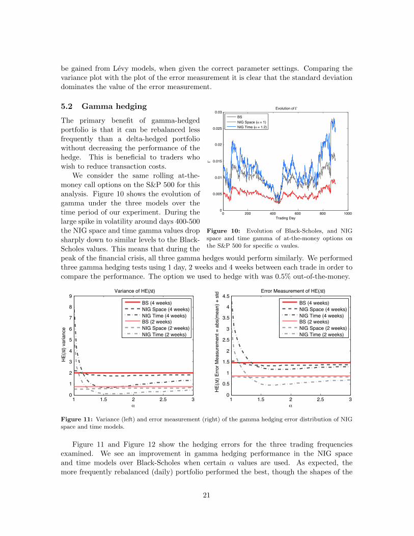
The primary benefit of gamma-hedgedportfolio is that it can be rebalanced lessfrequently than a delta-hedged portfoliowithout decreasing the performance of thehedge. This is beneficial to traders whowish to reduce transaction costs.

We consider the same rolling at-the-money call options on the S&P 500 for thisanalysis. Figure 10 shows the evolution ofgamma under the three models over thetime period of our experiment. During thelarge spike in volatility around days 400-500the NIG space and time gamma values dropsharply down to similar levels to the Black-Scholes values. This means that during thepeak of the financial crisis, all three gamma hedges would perform similarly. We performedthree gamma hedging tests using 1 day, 2 weeks and 4 weeks between each trade in order tocompare the performance. The option we used to hedge with was 0.5% out-of-the-money.

1 1.5 2 2.5 30

1

2

3

4

5

6

7

8

9

α

HE(Δt

) var

ianc

e

Variance of HE(Δt)

1 1.5 2 2.5 30

0.5

1

1.5

2

2.5

3

3.5

4

4.5

α

HE(Δt

) Erro

r Mea

sure

men

t = a

bs(m

ean)

+ s

td Error Measurement of HE(Δt)

BS (4 weeks)NIG Space (4 weeks)NIG Time (4 weeks)BS (2 weeks)NIG Space (2 weeks)NIG Time (2 weeks)

BS (4 weeks)NIG Space (4 weeks)NIG Time (4 weeks)BS (2 weeks)NIG Space (2 weeks)NIG Time (2 weeks)

Figure 11: Variance (left) and error measurement (right) of the gamma hedging error distribution of NIGspace and time models.

Figure 11 and Figure 12 show the hedging errors for the three trading frequenciesexamined. We see an improvement in gamma hedging performance in the NIG spaceand time models over Black-Scholes when certain α values are used. As expected, themore frequently rebalanced (daily) portfolio performed the best, though the shapes of the

21

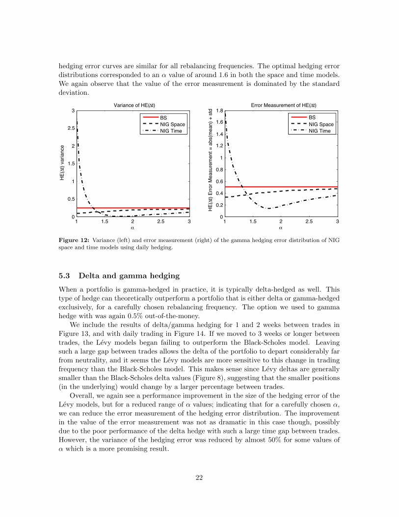
hedging error curves are similar for all rebalancing frequencies. The optimal hedging errordistributions corresponded to an α value of around 1.6 in both the space and time models.We again observe that the value of the error measurement is dominated by the standarddeviation.

1 1.5 2 2.5 30

0.5

1

1.5

2

2.5

3

α

HE(Δt

) var

ianc

e

Variance of HE(Δt)

1 1.5 2 2.5 30

0.2

0.4

0.6

0.8

1

1.2

1.4

1.6

1.8

α

HE(Δt

) Erro

r Mea

sure

men

t = a

bs(m

ean)

+ s

td

Error Measurement of HE(Δt)

BSNIG SpaceNIG Time

BSNIG SpaceNIG Time

Figure 12: Variance (left) and error measurement (right) of the gamma hedging error distribution of NIGspace and time models using daily hedging.

5.3 Delta and gamma hedging

When a portfolio is gamma-hedged in practice, it is typically delta-hedged as well. Thistype of hedge can theoretically outperform a portfolio that is either delta or gamma-hedgedexclusively, for a carefully chosen rebalancing frequency. The option we used to gammahedge with was again 0.5% out-of-the-money.

We include the results of delta/gamma hedging for 1 and 2 weeks between trades inFigure 13, and with daily trading in Figure 14. If we moved to 3 weeks or longer betweentrades, the Levy models began failing to outperform the Black-Scholes model. Leavingsuch a large gap between trades allows the delta of the portfolio to depart considerably farfrom neutrality, and it seems the Levy models are more sensitive to this change in tradingfrequency than the Black-Scholes model. This makes sense since Levy deltas are generallysmaller than the Black-Scholes delta values (Figure 8), suggesting that the smaller positions(in the underlying) would change by a larger percentage between trades.

Overall, we again see a performance improvement in the size of the hedging error of theLevy models, but for a reduced range of α values; indicating that for a carefully chosen α,we can reduce the error measurement of the hedging error distribution. The improvementin the value of the error measurement was not as dramatic in this case though, possiblydue to the poor performance of the delta hedge with such a large time gap between trades.However, the variance of the hedging error was reduced by almost 50% for some values ofα which is a more promising result.

22

1.5 2 2.5 3 3.5 40

0.5

1

1.5

2

α

HE(Δt

) var

ianc

e

Variance of HE(Δt)

1.5 2 2.5 3 3.5 4 4.50

0.5

1

1.5

2

2.5

αH

E(Δt

) Erro

r Mea

sure

men

t = a

bs(m

ean)

+ s

td

Error Measurement of HE(Δt)

BS (2 weeks)NIG Space (2 weeks)NIG Time (2 weeks)BS (1 week)NIG Space (1 week)NIG Time (1 week)

BS (2 weeks)NIG Space (2 weeks)NIG Time (2 weeks)BS (1 week)NIG Space (1 week)NIG Time (1 week)

Figure 13: Variance (left) and error measurement (right) of the delta/gamma hedging error distributionof NIG space and time models.

2 2.5 3 3.5 4 4.5

2

3

4

5

6

7

8

9x 10−3

α

HE(Δt

) var

ianc

e

Variance of HE(Δt)

2 2.5 3 3.5 40.06

0.08

0.1

0.12

0.14

0.16

α

HE(Δt

) Erro

r Mea

sure

men

t = a

bs(m

ean)

+ s

td

Error Measurement of HE(Δt)

BSNIG SpaceNIG Time

BSNIG SpaceNIG Time

Figure 14: Variance (left) and error measurement (right) of the delta/gamma hedging error distributionof NIG space and time models using daily rebalancing.

23

6 Barrier pricing performance

As a test of how the prices of barrier options are affected by which pricing model andwhich implied volatility is used, we calculate the prices of theoretical barrier call optionson AAPL stock using the implied volatility values from the asymmetric “smirk” NIG spacecase (Figure 6). We perform four sets of Monte Carlo simulations using vanilla call optionprices as a control variate to reduce the variance of the sample payoffs. The four sets ofsimulations performed were configured as follows:

1. Geometric Brownian motion price process using σBS(K)

2. Geometric Brownian motion price process using σNIG(K)

3. NIG space price process using σBS(K)

4. NIG space price process using σNIG(K)

The parameter settings for the simulations were:

S0 = 264.08, r = 2%, q = 0, T = 178/365,K = 230, 240, . . . , 360, 370, Bup = 350, Bdown = 250.

The barrier levels Bup and Bdown were chosen to ensure that the barrier option priceswere not particularly one-sided. Recall the no-arbitrage condition that the sum of the pricesof an “in” and ”out” pair of options should equal the price of a vanilla option. This meansthat a decrease in the price of one member of the pair results in an increase in the price ofthe other member.

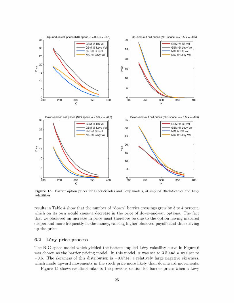
Our primary interest is in examining how moving from implied Black-Scholes volatilityto implied Levy volatility affects the barrier prices. Pricing the options in the four waysdescribed will allow us to isolate the effects of the model (kurtosis, skewness, etc. . . ) fromthe effects of the volatility. We create four separate pricing graphs for up-and-in, up-and-out, down-and-in, and down-and-out barrier call options. Figure 15 looks at the barrierprices obtained by using both a geometric Brownian motion price process and a Levy priceprocess, with both the Black-Scholes and Levy implied volatilities. Table 4 contains thepercentage values of barrier crossings that were observed in the simulations.

6.1 Geometric Brownian motion price process

We first discuss the prices obtained using the geometric Brownian motion price process.We see in Figure 15 that in the case of “up” barrier options, the increase in volatility fromswitching to implied Levy volatility caused an increase in the price of up-and-in optionsand a slight decrease in the price of up-and-out options. This makes intuitive sense becausea higher volatility makes the stock price more likely to cross the barrier, thus making “in”options more valuable and “out” options less valuable. The first two rows of Table 4 showan increase of approximately a 7–8% in the percentage of “up” barrier crossings observedafter switching from Black-Scholes to Levy volatility.

The results are slightly different in the case of the “down” options. The Levy volatilityprices were higher for both the down-and-in and the down-and-out calls. In this case the

24

200 250 300 350 4000

5

10

15

20

25

30

35Up−and−in call prices (NIG space, α = 3.5, κ = −0.5)

K

Pric

e

200 250 300 350 4000

5

10

15

20

25

30Up−and−out call prices (NIG space, α = 3.5, κ = −0.5)

K

Pric

e

200 250 300 350 4000

5

10

15

20

25

30Down−and−in call prices (NIG space, α = 3.5, κ = −0.5)

K

Pric

e

200 250 300 350 4000

5

10

15

20

25

30

35Down−and−out call prices (NIG space, α = 3.5, κ = −0.5)

K

Pric

e

GBM @ BS volGBM @ Levy VolNIG @ BS volNIG @ Levy Vol

GBM @ BS volGBM @ Levy VolNIG @ BS volNIG @ Levy Vol

GBM @ BS volGBM @ Levy VolNIG @ BS volNIG @ Levy Vol

GBM @ BS volGBM @ Levy VolNIG @ BS volNIG @ Levy Vol

Figure 15: Barrier option prices for Black-Scholes and Levy models, at implied Black-Scholes and Levyvolatilities.

results in Table 4 show that the number of “down” barrier crossings grew by 3 to 4 percent,which on its own would cause a decrease in the price of down-and-out options. The factthat we observed an increase in price must therefore be due to the option having matureddeeper and more frequently in-the-money, causing higher observed payoffs and thus drivingup the price.

6.2 Levy price process

The NIG space model which yielded the flattest implied Levy volatility curve in Figure 6was chosen as the barrier pricing model. In this model, α was set to 3.5 and κ was set to−0.5. The skewness of this distribution is −0.5714; a relatively large negative skewness,which made upward movements in the stock price more likely than downward movements.

Figure 15 shows results similar to the previous section for barrier prices when a Levy

25

Table 4: Percentage of Monte Carlo simulations where barrier was crossed for each type of barrier optionand pricing configuration.

Up-and-in Up-and-out Down-and-in Down-and-out

GBM @ BS vol 17.07 16.97 79.58 79.70GBM @ Levy vol 24.13 24.39 83.77 83.29

NIG @ BS vol 8.91 9.04 62.01 62.10NIG @ Levy vol 14.98 14.79 66.51 66.27

price process is used. We see in the case of “up” options that the higher (implied Levy )volatility increased the value of the up-and-in options and decreased slightly the value ofthe up-and-out options. This was coupled with a 5–6% increase in the number of barriercrossings. In the case of “down” options we observe that the negative skewness caused thenumber of barrier crossing events that occurred to increase by only 3–4%. So the increasein price when using Levy volatility must again be caused by the options finishing deeperin-the-money on average. This was helped by the large negative skewness our distributionwas calibrated with.

The effect on the prices by switching to a Levy process was much more significant thanthe effect of the volatility. In Figure 15 we see in both the “up” and ”down” cases that theswitch to a Levy process caused a decrease in the price of “in” options and an increase ofequal value in the price of ”out” options. This suggests a decrease in the number of barriercrossings upon switching to the Levy process. Table 4 shows that in all 8 cases (4 types ofbarrier option, 2 types of volatility), the move to a Levy process did dramatically decreasethe number of observed barrier crossings.

The decrease in barrier crossings is surprising given that our Levy process has a skewnessof −0.5714 and a kurtosis of 3.807; slightly higher than the normal distribution. We wouldexpect the move to a heavier tailed distribution to cause more barrier crossings. The factthat we observed less crossings implies that the NIG process we used tends to remain closerto S0 over the course of the simulations compared to a geometric Brownian motion.

7 Conclusion

By using the concept of implied Levy volatility first introduced by Corcuera et. al. in [6],we have shown that switching to a more flexible Levy distribution allows us to performseveral market functions more accurately than under the Black-Scholes model.

We first tested the performance of implied Levy volatility with real market data. Itwas demonstrated that the curvature of an implied volatility plot could be minimized witha properly calibrated Levy model. The additional degrees of freedom allowed us to useasymmetric distributions with heavier tails, which better fit the return distributions ob-served historically. This gave improvements over implied Black-Scholes volatility smilesand smirks, with the smirk case showing the greatest improvement by flattening the curvealmost completely.

It was shown that one can calibrate a Levy model such that the absolute mean andvariance of the hedging error are lower than those values obtained by the Black-Scholes

26

model for delta, gamma and delta/gamma hedging. Even using data covering the 2007financial crisis, we saw a reduction in the hedging error of as much as 50% in certain deltaand gamma hedging models. The ability to reduce hedging error is desirable to any optiontrader as it can effectively minimize losses due to the errors that can arise from hedgingdiscretely. This can in turn lead to lower economic capital requirements and thus highermargins for profits.

Lastly we used the flattened volatility curve obtained earlier to analyze the effect ofvolatility on the price of barrier options. A flatter volatility curve is desirable becauseit eliminates the problem of which implied volatility one should input into the pricingfunction; the volatility corresponding to the strike price, the barrier level or perhaps someaverage of the two. We saw changes in our Monte Carlo barrier prices caused by changesin the percentage of barrier crossings, and also how deep and how frequently the optionsfinished in-the-money. If barrier options are priced using a model which is more accuratelycalibrated to the market, these changes in barrier crossings and moneyness should reflectmore closely the type of behaviour that is observed historically.

8 Future Work

The results we have discussed here were for a normal inverse Gaussian process, but theprocedures we used can be applied using any Levy process for which the characteristicfunction is computable. This includes, for instance the Meixner, variance gamma, CGMY,and generalized tempered stable processes. We could possibly improve performance furtherby seeing how each of these models compare at flattening the implied volatility surface,especially in the case of a “smile”, where the results we saw showed room for improvement.

There are other forms of hedging which can be expanded to Levy models. These mostnotably include theta; sensitivity of the option value with respect to time, and vega; thesensitivity with respect to volatility. By formulating the theta and vega of an option underthe Carr-Madan framework, we can compare the performance of a broader range of hedgingstrategies.

Lastly, the techniques we have for pricing barrier options using implied Levy volatilitycan be applied to any other exotic option where there is some uncertainty in which volatilityto use for pricing. The change in performance upon switching to implied Levy volatilitycould be compared with what was seen in barrier options which could provide deeperunderstanding of how the volatility affects the value of exotic options.

27

References

[1] Back, K. (2005) A Course in Derivative Securities. Springer-Verlag Berlin Heidelberg.

[2] Barndorff-Nielsen, O.E. (1998) Processes of Normal Inverse Gaussian Type. Financeand Stochastics, 2, 41-68.

[3] Black, F. and Scholes, M. (1973) The Pricing of Options and Corporate Liabilities.Journal of Political Economy, 81, 637-654.

[4] Carr, P. and Madan, D. (1999) Option Valuation using the Fast Fourier Transform.Journal of Computational Finance, 2, 61-73.

[5] Cont, R. and Tankov, P. (2003) Financial Modelling with Jump Processes. Chapman &Hall / CRC Press.

[6] Corcuera, J.M., Guillaume, F., Leoni, P., Schoutens, W. (2009) Implied Levy Volatility.Journal of Quantitative Finance, 9, 383-393.

[7] Schoutens, W. (2003) Levy Processes in Finance: Pricing Financial Derivatives. JohnWiley & Sons Ltd.

[8] Schoutens, W. and Symens, S. (2003) The Pricing of Exotic Options by Monte CarloSimulations in a Levy Market with Stochastic Volatility. Journal for Theoretical andApplied Finance, 6, 839-864.

[9] Shreve, S. (2004) Stochastic Calculus for Finance II. Springer Science + Business Media,LLC.

28