a parsimonious arbitrage-free implied volatility...

A parsimonious arbitrage-free implied volatility parameterization withapplication to the valuation of volatility derivatives

Jim GatheralGlobal Derivatives & Risk Management 2004MadridMay 26, 2004

Jim Gatheral, Merrill Lynch, May-2004

The opinions expressed in this presentation are those of the author alone,and do not necessarily reflect the views of of Merrill Lynch, itssubsidiaries or affiliates.


Outline of this talk

n Roger Lee’s moment formulan A stochastic volatility inspired (SVI) pararameterization of the implied

volatility surfacen No-arbitrage conditionsn SVI fits to market datan SVI fits to theoretical modelsn Carr-Lee valuation of volatility derivatives under the zero correlation

assumptionn Valuation of volatility derivatives in the general case


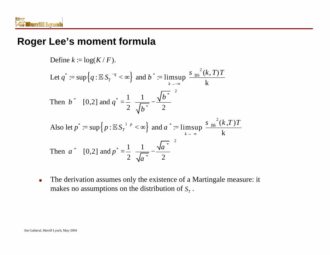
Roger Lee’s moment formula

{ }

{ }

2* * BS

2*

* *

*

21* * BS

** *

*

Define : log( / ).

( , )Let : sup : and : limsup

k

1 1Then [0,2] and

2 2

( , )Also let : sup : and : limsup

k

1 1Then [0,2] and 2 2

qT

k

pT

k

k K F

k T Tq q S

q

k T Tp p S

p

σβ

ββ

β

σα

ααα

−

→−∞

+

→+∞

=

= < ∞ =

∈ = −

= < ∞ =

∈ = −

E

E2

n The derivation assumes only the existence of a Martingale measure: itmakes no assumptions on the distribution of .TS


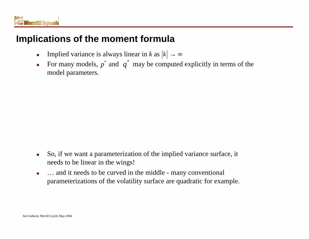
Implications of the moment formula

n Implied variance is always linear in k asn For many models, and may be computed explicitly in terms of the

model parameters.

n So, if we want a parameterization of the implied variance surface, itneeds to be linear in the wings!

n … and it needs to be curved in the middle - many conventionalparameterizations of the volatility surface are quadratic for example.

k → ∞*p *q


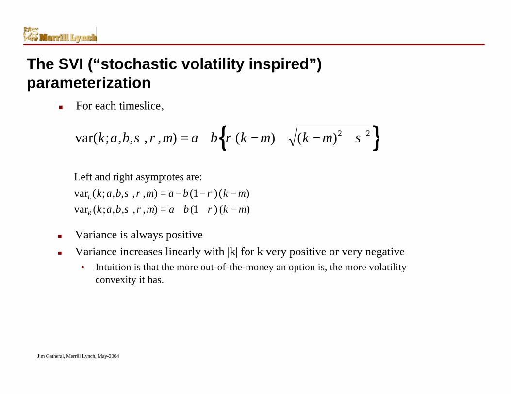
var( ; , , , , ) ( ) ( )k a b m a b k m k mσ ρ ρ σ= + − + − +2 2{ }Left and right asymptotes are:

var ( ; , , , , ) ( ) ( )var ( ; , , , , ) ( ) ( )

L

R

k a b m a b k mk a b m a b k m

σ ρ ρσ ρ ρ

= − − −= + + −

11

The SVI (“stochastic volatility inspired”)parameterization

n Variance is always positiven Variance increases linearly with |k| for k very positive or very negative

• Intuition is that the more out-of-the-money an option is, the more volatilityconvexity it has.

n For each timeslice,


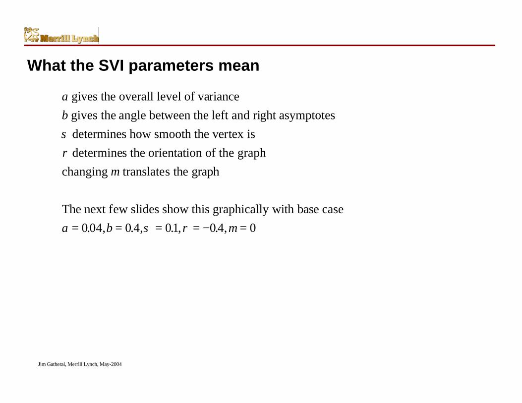
ab

m

a b m

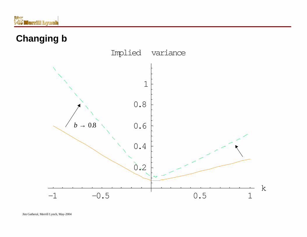
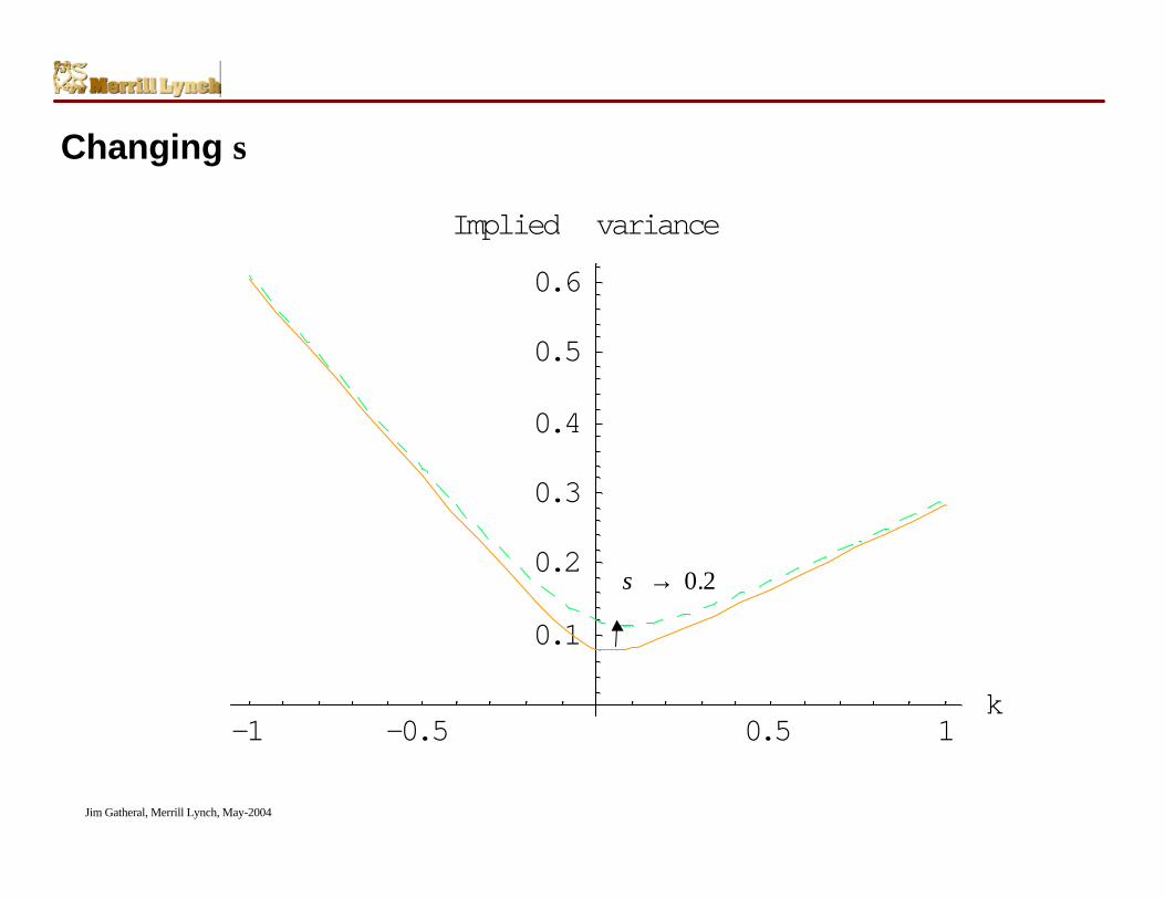
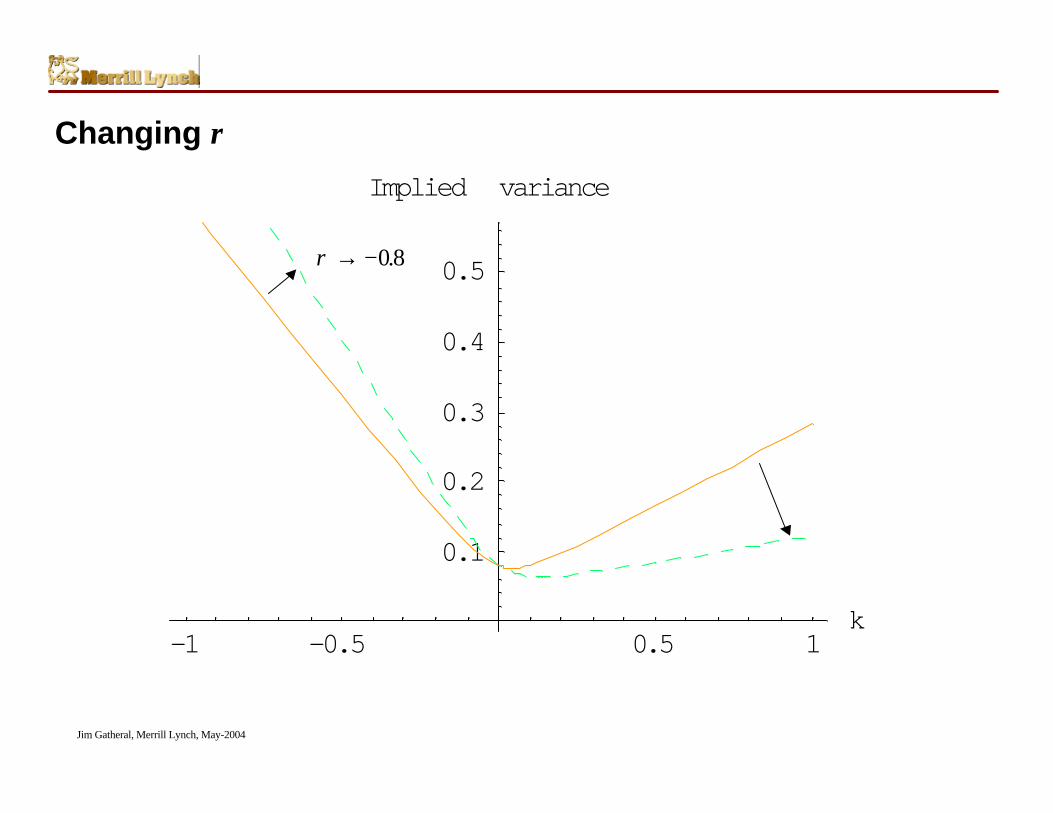
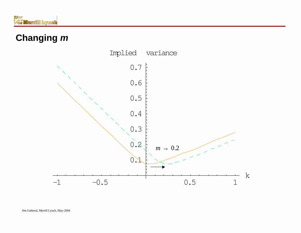
gives the overall level of variance gives the angle between the left and right asymptotes determines how smooth the vertex is determines the orientation of the graph

changing translates the graph

The next few slides show this graphically with base case

σρ

σ ρ= = = = − =0 04 0 4 01 0 4 0. , . , . , . ,

What the SVI parameters mean


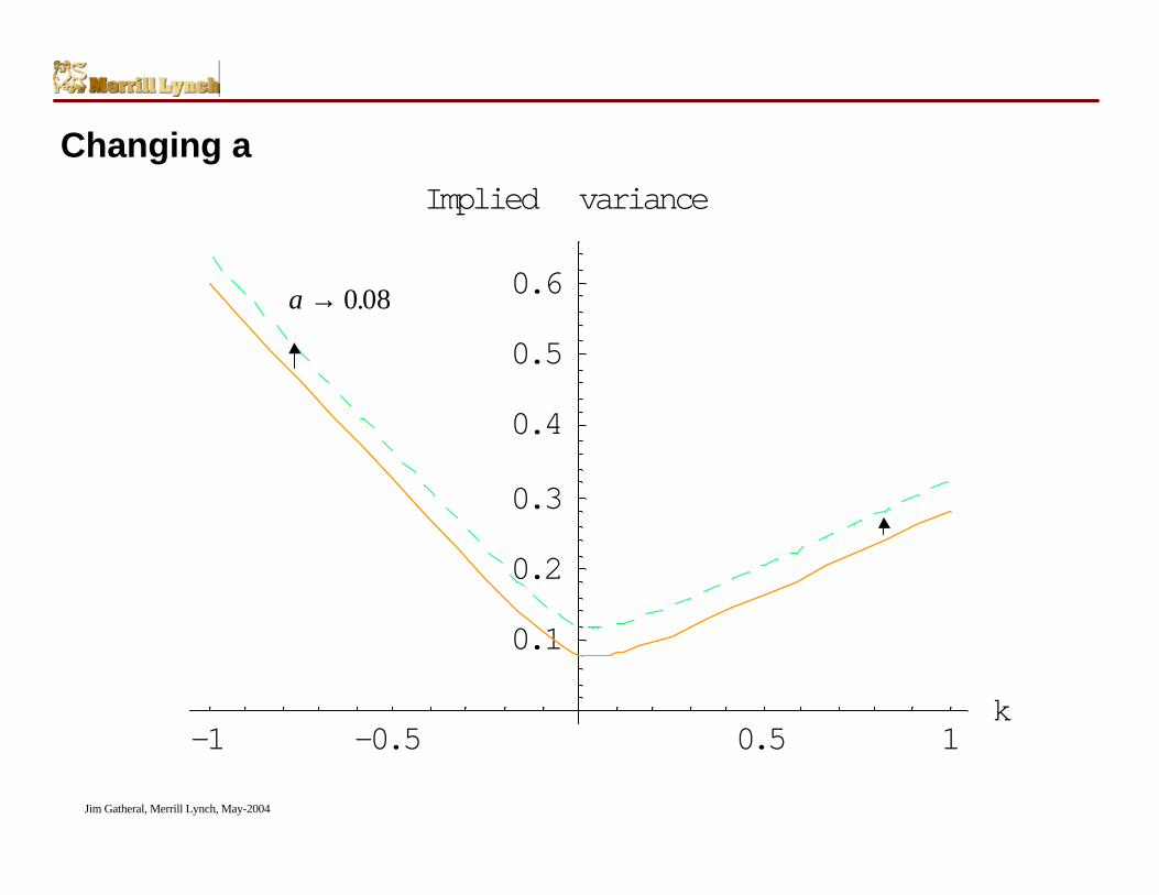
-1 -0.5 0.5 1k

0.1

0.2

0.3

0.4

0.5

0.6

Implied variance

a → 0 08.

Changing a


-1 -0.5 0.5 1k

0.2

0.4

0.6

0.8

1

Implied variance

b → 0 8.

Changing b


-1 -0.5 0.5 1k

0.1

0.2

0.3

0.4

0.5

0.6

Implied variance

σ → 0 2.

Changing σ


-1 -0.5 0.5 1k

0.1

0.2

0.3

0.4

0.5

Implied variance

ρ → −08.

Changing ρ


-1 -0.5 0.5 1k

0.1

0.2

0.3

0.4

0.5

0.6

0.7

Implied variance

m → 0 2.

Changing m


Preventing arbitrage

n In practice, if SVI is fitted to actual option price data, negative verticalspreads never arise. In terms of the SVI (implied variance fit)parameters, the condition is

n It turns out that if there are no negative vertical spreads, negativebutterflies are also excluded.

n In contrast, it is not obvious how to prevent negative time spreads. Wenow show what conditions a parameterization needs to satisfy to excludearbitrage between expirations (calendar spread arbitrage).

( ) 41b

Tρ+ ≤


Necessary and sufficient condition for no calendarspread arbitrage

n First we note that for any Martingale and it is easy to showthat

n Now consider the non-discounted values and of two options withstrikes and and expirations and with . Suppose the twooptions have the same moneyness so that

( ) ( )2 1t tX L X L

+ +− ≥ −E E

2 1t t≥tX

2 1t t>1C 2C

1K 2K 1t 2t

1 2

1 2

K Kk

F F= ≡

n Consider the martingale . Then, in the absence of arbitrage,we must have

/t t tX S F≡

( ) ( )2 1

2 1

2 1

1 1t t

C CX k X k

K k k K+ +

= − ≥ − == E En So, keeping the moneyness constant, option prices are non-decreasing in

time to expiration.


Derivation of no arbitrage condition continued

n Letn The Black-Scholes formula for the non-discounted value of an option

may be expressed in the form with strictly increasing inthe total implied variance .

n It follows that for fixed k, we must have the total implied variancenon-decreasing with respect to time to expiration.

( )2,t BSw k t tσ≡

( , )BS tC k w BSCtw

tw


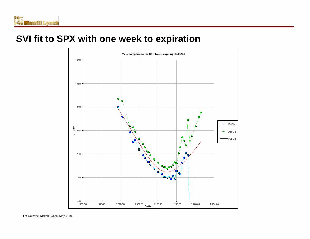
SVI fit to SPX with one week to expirationVols comparison for SPX Index expiring 05/21/04

10%

15%

20%

25%

30%

35%

40%

900.00 950.00 1,000.00 1,050.00 1,100.00 1,150.00 1,200.00 1,250.00Strike

Vo

lati

lity

Bid Vol

Ask Vol

SVI Vol


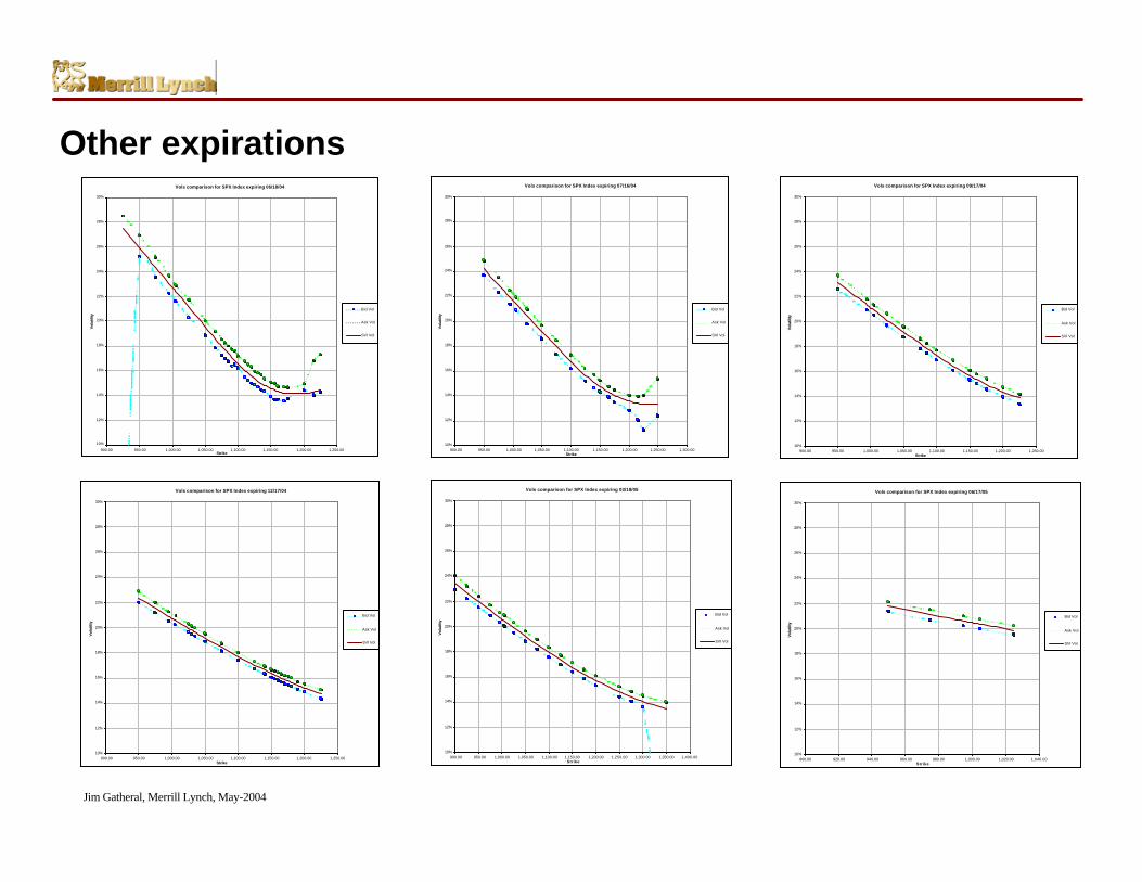
Other expirationsVols comparison for SPX Index expiring 06/18/04

10%

12%

14%

16%

18%

20%

22%

24%

26%

28%

30%

900.00 950.00 1,000.00 1,050.00 1,100.00 1,150.00 1,200.00 1,250.00Strike

Vol

atili

ty

Bid Vol

Ask Vol

SVI Vol

Vols comparison for SPX Index expiring 07/16/04

10%

12%

14%

16%

18%

20%

22%

24%

26%

28%

30%

900.00 950.00 1,000.00 1,050.00 1,100.00 1,150.00 1,200.00 1,250.00 1,300.00Strike

Vol

atili

ty

Bid Vol

Ask Vol

SVI Vol


10%

12%

14%

16%

18%

20%

22%

24%

26%

28%

30%

900.00 950.00 1,000.00 1,050.00 1,100.00 1,150.00 1,200.00 1,250.00Strike

Vol

atili

ty

Bid Vol

Ask Vol

SVI Vol


10%

12%

14%

16%

18%

20%

22%

24%

26%

28%

30%

900.00 950.00 1,000.00 1,050.00 1,100.00 1,150.00 1,200.00 1,250.00Strike

Vol

atili

ty

Bid Vol

Ask Vol

SVI Vol


10%

12%

14%

16%

18%

20%

22%

24%

26%

28%

30%

900.00 950.00 1,000.00 1,050.00 1,100.00 1,150.00 1,200.00 1,250.00 1,300.00 1,350.00 1,400.00Strike

Vol

atili

ty

Bid Vol

Ask Vol

SVI Vol


10%

12%

14%

16%

18%

20%

22%

24%

26%

28%

30%

900.00 920.00 940.00 960.00 980.00 1,000.00 1,020.00 1,040.00Strike

Vol

atili

ty

Bid Vol

Ask Vol

SVI Vol


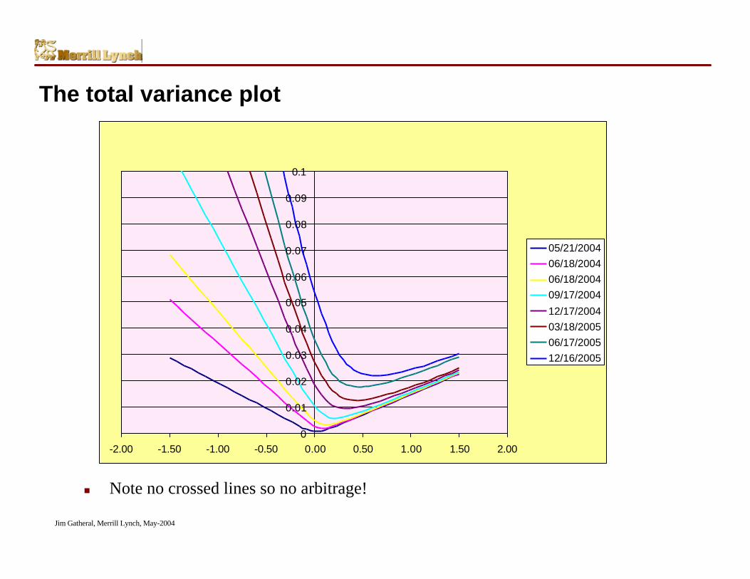
The total variance plot

0

0.01

0.02

0.03

0.04

0.05

0.06

0.07

0.08

0.09

0.1

-2.00 -1.50 -1.00 -0.50 0.00 0.50 1.00 1.50 2.00

05/21/200406/18/200406/18/200409/17/2004

12/17/200403/18/200506/17/200512/16/2005

n Note no crossed lines so no arbitrage!


Review of the work of Schoutens et al.

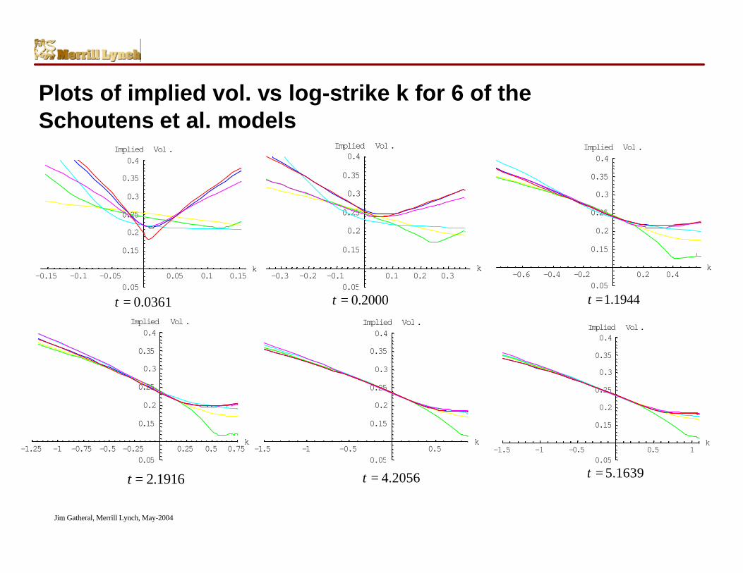
n In their recent Wilmott Magazine paper, Schoutens, Simons and Tistaertcarefully fitted 7 different models to the STOXX50 index option marketobserved on 7-Oct-2003.

n The models fitted were• HEST, HESJ, BNS, VG-CIR, VG-OUΓ, NIG-CIR, NIG-OUΓ

n These models represent a range of quite different dynamics. Forexample, HEST is a pure stochastic volatility model and VG-CIR is apure jump model with subordinated time.


-0.6 -0.4 -0.2 0.2 0.4k

0.05

0.15

0.2

0.25

0.3

0.35

0.4Implied Vol.

-0.3 -0.2 -0.1 0.1 0.2 0.3k

0.05

0.15

0.2

0.25

0.3

0.35

0.4Implied Vol.

-0.15 -0.1 -0.05 0.05 0.1 0.15k

0.05

0.15

0.2

0.25

0.3

0.35

0.4Implied Vol.

-1.25 -1 -0.75 -0.5 -0.25 0.25 0.5 0.75k

0.05

0.15

0.2

0.25

0.3

0.35

0.4Implied Vol.

-1.5 -1 -0.5 0.5k

0.05

0.15

0.2

0.25

0.3

0.35

0.4Implied Vol.

-1.5 -1 -0.5 0.5 1k

0.05

0.15

0.2

0.25

0.3

0.35

0.4Implied Vol.

Plots of implied vol. vs log-strike k for 6 of theSchoutens et al. models

0.0361t = 0.2000t = 1.1944t =

2.1916t = 5.1639t =4.2056t =


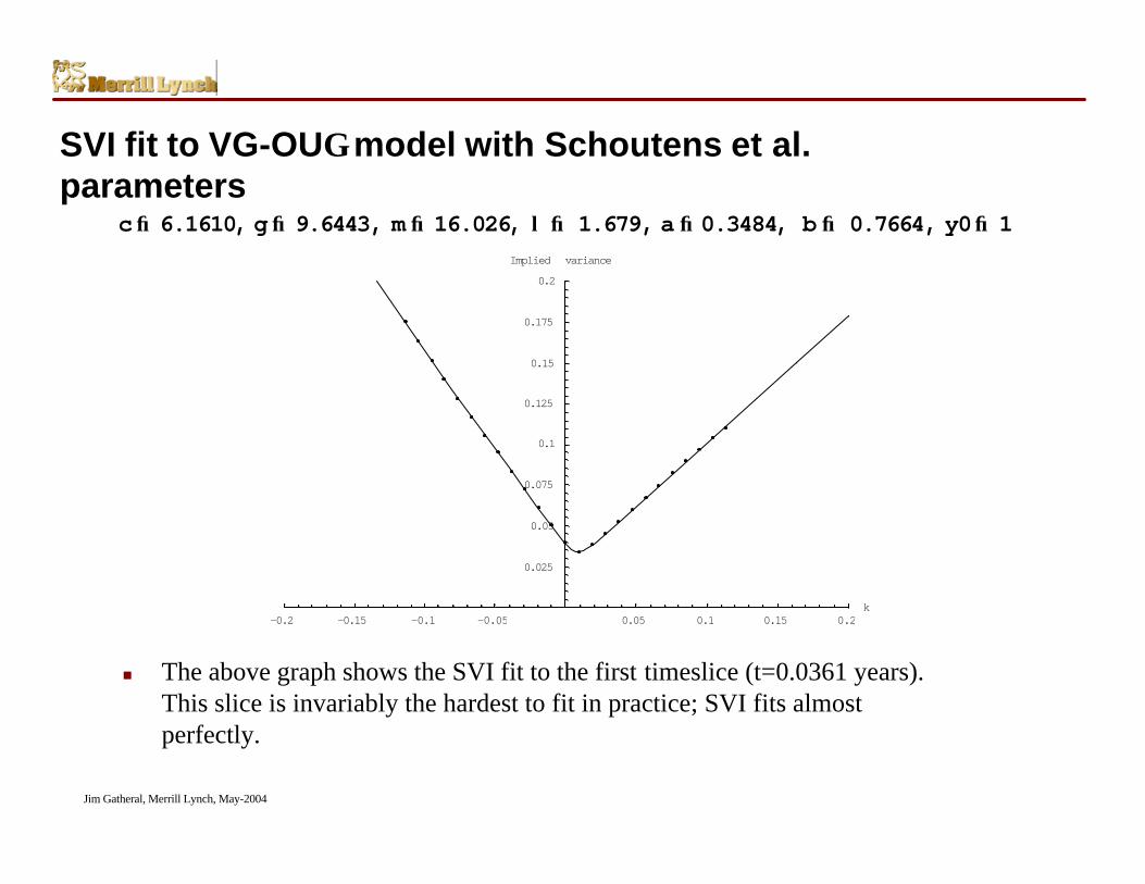
SVI fit to VG-OUΓ model with Schoutens et al.parameters

n The above graph shows the SVI fit to the first timeslice (t=0.0361 years).This slice is invariably the hardest to fit in practice; SVI fits almostperfectly.

-0.2 -0.15 -0.1 -0.05 0.05 0.1 0.15 0.2k

0.025

0.05

0.075

0.1

0.125

0.15

0.175

0.2

Implied variance

c® 6.1610, g® 9.6443, m ® 16.026, l ® 1.679, a ® 0.3484, b ® 0.7664, y0® 1


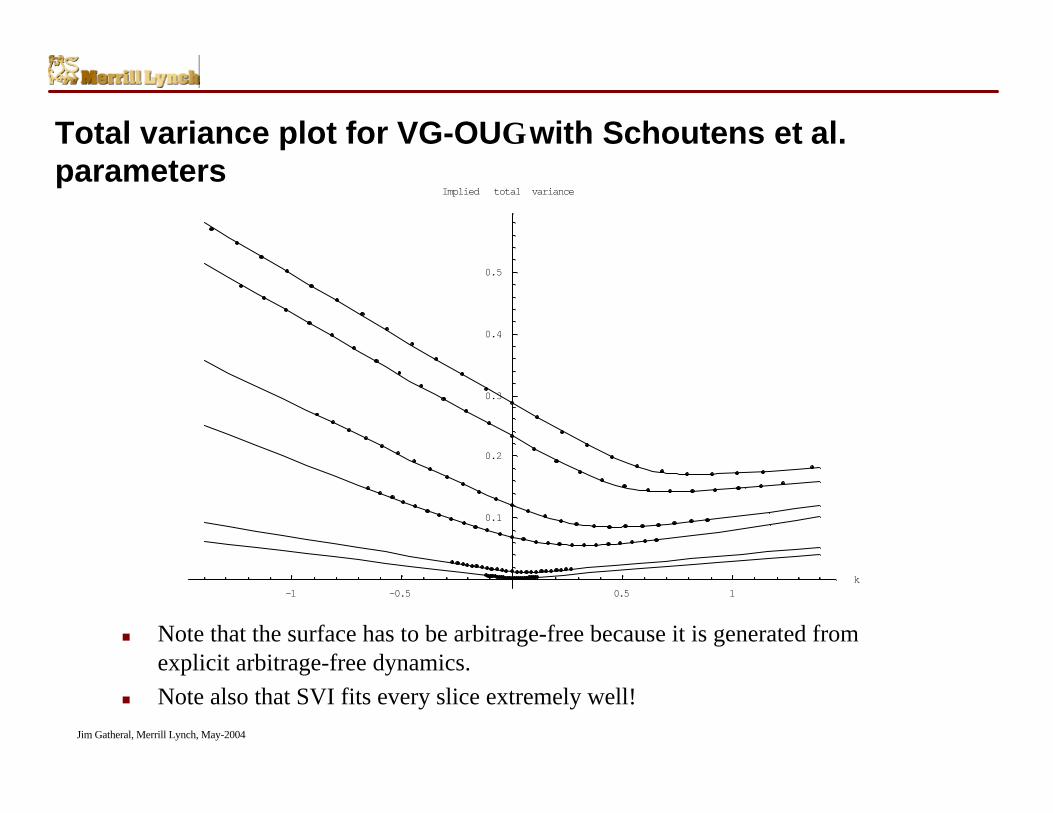
Total variance plot for VG-OUΓ with Schoutens et al.parameters

n Note that the surface has to be arbitrage-free because it is generated fromexplicit arbitrage-free dynamics.

n Note also that SVI fits every slice extremely well!

-1 -0.5 0.5 1k

0.1

0.2

0.3

0.4

0.5

Implied total variance


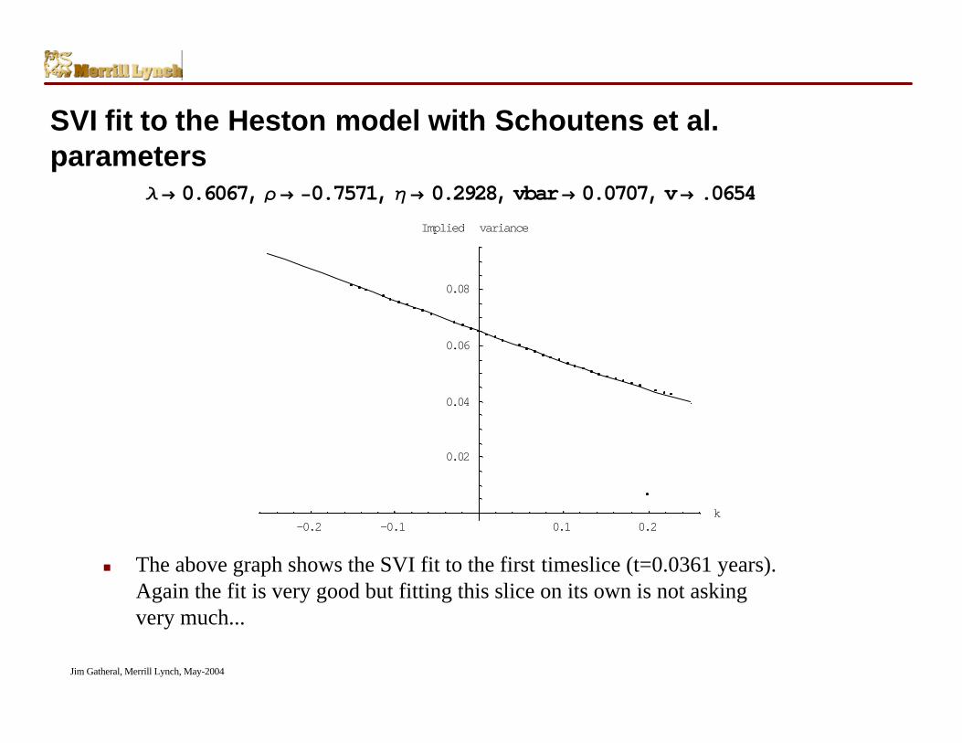
SVI fit to the Heston model with Schoutens et al.parameters

n The above graph shows the SVI fit to the first timeslice (t=0.0361 years).Again the fit is very good but fitting this slice on its own is not askingvery much...

λ → 0.6067, ρ → −0.7571, η → 0.2928, vbar→ 0.0707, v→ .0654

-0.2 -0.1 0.1 0.2k

0.02

0.04

0.06

0.08

Implied variance


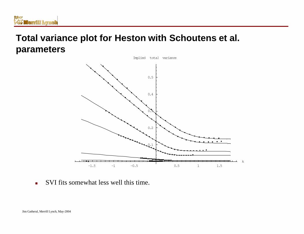
Total variance plot for Heston with Schoutens et al.parameters

n SVI fits somewhat less well this time.

-1.5 -1 -0.5 0.5 1 1.5k

0.1

0.2

0.3

0.4

0.5

Implied total variance


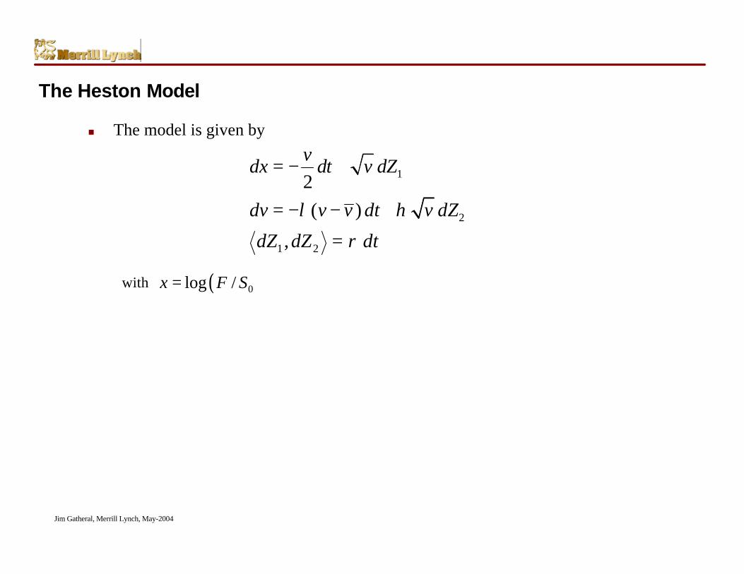
The Heston Model

n The model is given by

with

1

2

1 2

2( )

,

vdx dt v dZ

dv v v dt v dZ

dZ dZ dt

λ η

ρ

= − +

= − − +

=

( )0log /x F S=


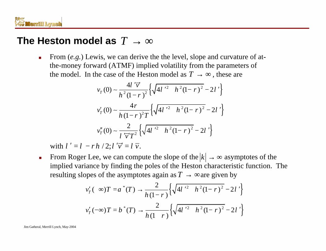
The Heston model as

n From (e.g.) Lewis, we can derive the the level, slope and curvature of at-the-money forward (ATMF) implied volatility from the parameters ofthe model. In the case of the Heston model as , these are

T → ∞

withn From Roger Lee, we can compute the slope of the asymptotes of the

implied variance by finding the poles of the Heston characteristic function. Theresulting slopes of the asymptotes again as are given by

k → ∞

{ }{ }

{ }

2 2 22 2

2 2 22

2 2 22

4(0) 4 (1 ) 2

(1 )4

(0) 4 (1 ) 2(1 )2

(0) 4 (1 ) 2

T

T

T

vv

vT

vv T

λλ η ρ λ

η ρρ λ η ρ λ

η ρ

λ η ρ λλ

′ ′′ ′+ − −

−

′ ′ ′+ − −−

′′ ′ ′+ − −′ ′

∼

∼

∼

{ }{ }

* 2 2 2

* 2 2 2

2( ) ( ) 4 (1 ) 2

(1 )2

( ) ( ) 4 (1 ) 2(1 )

T

T

v T T

v T T

α λ η ρ λη ρ

β λ η ρ λη ρ

′ ′ ′+∞ = → + − −−

′ ′ ′−∞ = → + − −+

/ 2; .v vλ λ ρη λ λ′ ′ ′= − =

T → ∞

T → ∞


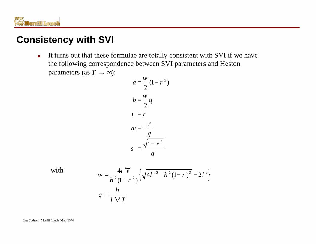
Consistency with SVI

n It turns out that these formulae are totally consistent with SVI if we havethe following correspondence between SVI parameters and Hestonparameters (as ):T → ∞

2

2

(1 )2

2

1

a

b

m

ωρ

ωθ

ρ ρρθ

ρσ

θ

= −

=

=

= −

−=

with { }2 2 22 2

44 (1 ) 2

(1 )v

v T

λω λ η ρ λ

η ρη

θλ

′ ′′ ′= + − −

−

=′ ′


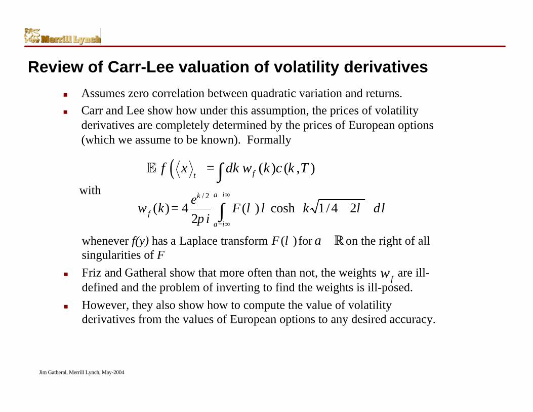
Review of Carr-Lee valuation of volatility derivatives

n Assumes zero correlation between quadratic variation and returns.n Carr and Lee show how under this assumption, the prices of volatility

derivatives are completely determined by the prices of European options(which we assume to be known). Formally

whenever f(y) has a Laplace transform for on the right of allsingularities of F

n Friz and Gatheral show that more often than not, the weights are ill-defined and the problem of inverting to find the weights is ill-posed.

n However, they also show how to compute the value of volatilityderivatives from the values of European options to any desired accuracy.

( ) ( ) ( , )ftf x dk w k c k T= ∫E

fw

with / 2

( ) 4 ( ) cosh 1/4 22

a ik

fa i

ew k F k d

iλ λ λ λ

π

+ ∞

− ∞

= + ∫( )F λ a ∈R


Extension to non-zero correlation

n Suppose that (e.g.) Heston dynamics really drive the market.n We note that the values of volatility derivatives are independent of the

correlation between stock returns and volatility moves.n To compute the fair value of a volatility derivative, all we would need to

do is to set to zero and apply the inversion method described in Frizand Gatheral.

n This suggests the following general recipe:n Start with some parameterization of the volatility surface.n Noting that when is zero, the implied variance smile is symmetric

around k=0, rotate the curve keeping its overall level the same.• Although this step is intuitively clear, its meaning is far from precise and its

implementation is far from obvious

n Apply the Friz algorithm to compute the value of the volatilityderivative.

ρ

ρ


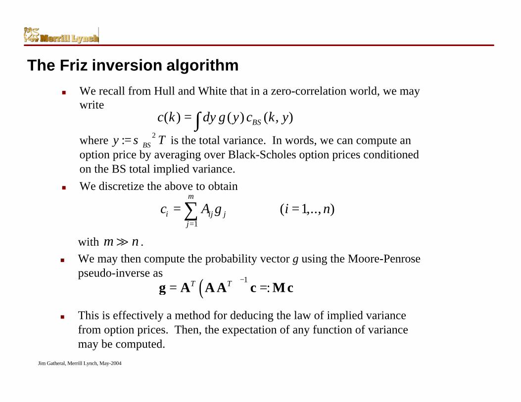
The Friz inversion algorithm

n We recall from Hull and White that in a zero-correlation world, we maywrite

( ) ( ) ( , )BSc k dy g y c k y= ∫where is the total variance. In words, we can compute anoption price by averaging over Black-Scholes option prices conditionedon the BS total implied variance.

n We discretize the above to obtain

2: BSy Tσ=

1

( 1,.., )m

i ij jj

c A g i n=

= =∑with .

n We may then compute the probability vector g using the Moore-Penrosepseudo-inverse as

m n?

( ) 1:T T −

= =g A A A c M c

n This is effectively a method for deducing the law of implied variancefrom option prices. Then, the expectation of any function of variancemay be computed.


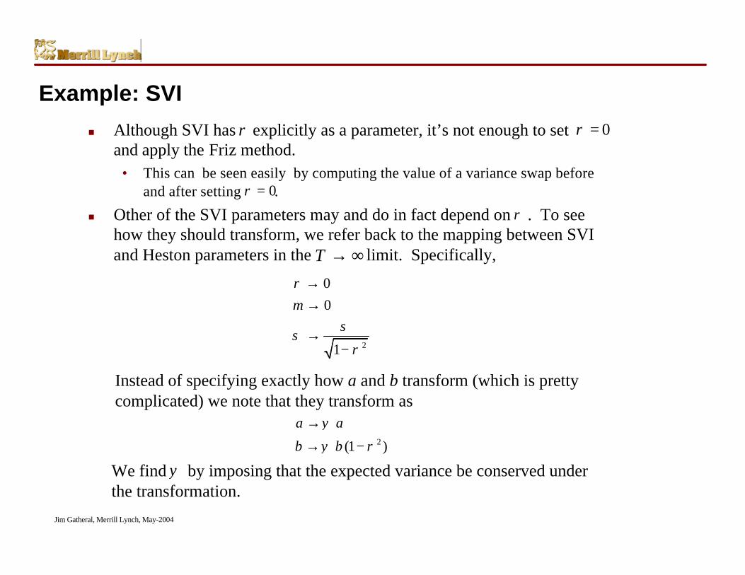
Example: SVI

n Although SVI has explicitly as a parameter, it’s not enough to setand apply the Friz method.

• This can be seen easily by computing the value of a variance swap beforeand after setting .

n Other of the SVI parameters may and do in fact depend on . To seehow they should transform, we refer back to the mapping between SVIand Heston parameters in the limit. Specifically,

ρ 0ρ =

0ρ =

ρ

T → ∞

2

00

1

mρ

σσ

ρ

→→

→−

Instead of specifying exactly how a and b transform (which is prettycomplicated) we note that they transform as

2(1 )

a a

b b

ψ

ψ ρ

→

→ −

We find by imposing that the expected variance be conserved underthe transformation.

ψ


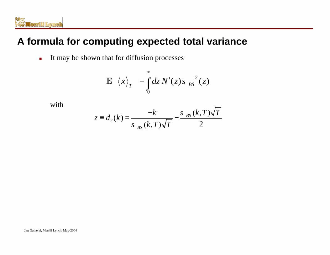
A formula for computing expected total variance

n It may be shown that for diffusion processes

2

0

( ) ( )BSTx dz N z zσ

∞

′ = ∫E

with

2( , )

( )2( , )

BS

BS

k T Tkz d k

k T Tσ

σ−

≡ = −


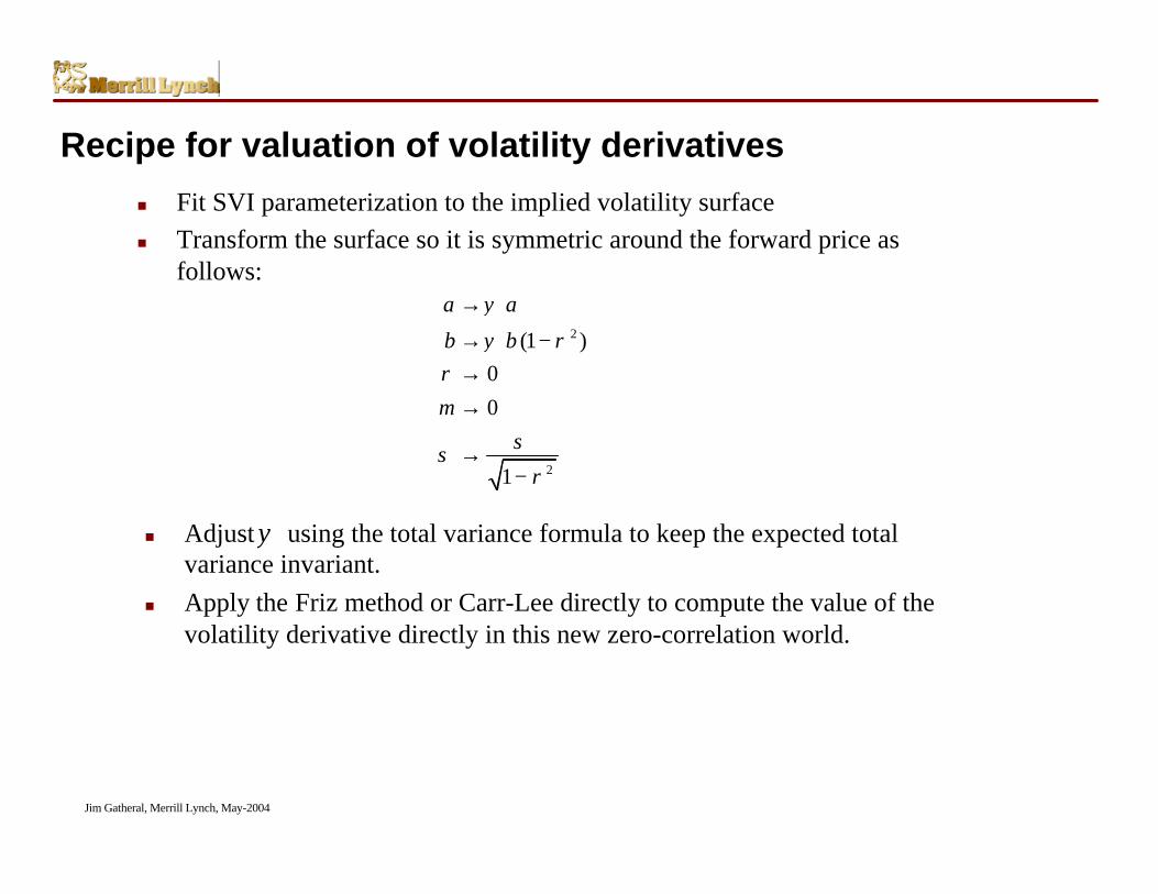
Recipe for valuation of volatility derivatives

n Fit SVI parameterization to the implied volatility surfacen Transform the surface so it is symmetric around the forward price as

follows:

2

2

(1 )00

1

a a

b b

m

ψ

ψ ρρ

σσρ

→

→ −→→

→−

n Adjust using the total variance formula to keep the expected totalvariance invariant.

n Apply the Friz method or Carr-Lee directly to compute the value of thevolatility derivative directly in this new zero-correlation world.

ψ


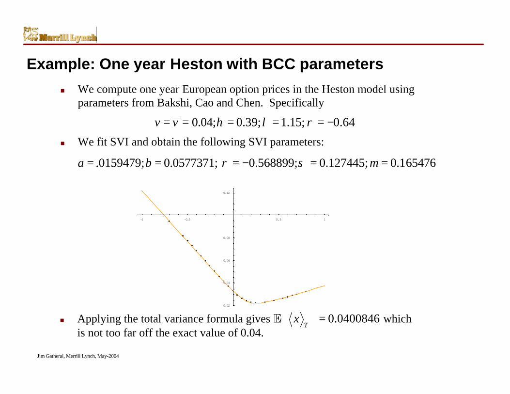
Example: One year Heston with BCC parameters

n We compute one year European option prices in the Heston model usingparameters from Bakshi, Cao and Chen. Specifically

0.04; 0.39; 1.15; 0.64v v η λ ρ= = = = = −

n We fit SVI and obtain the following SVI parameters:

-1 -0.5 0.5 1

0.02

0.04

0.06

0.08

0.12

.0159479; 0.0577371; 0.568899; 0.127445; 0.165476a b mρ σ= = = − = =

n Applying the total variance formula gives whichis not too far off the exact value of 0.04.

0.0400846T

x = E


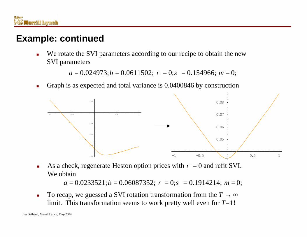
Example: continued

n We rotate the SVI parameters according to our recipe to obtain the newSVI parameters

n Graph is as expected and total variance is 0.0400846 by construction

-1 -0.5 0.5 1

0.05

0.06

0.07

0.08

-1 -0.5 0.5 1

0.02

0.04

0.06

0.08

0.12

n As a check, regenerate Heston option prices with and refit SVI.We obtain

0ρ =

0.0233521; 0.06087352; 0; 0.1914214; 0;a b mρ σ= = = = =

n To recap, we guessed a SVI rotation transformation from thelimit. This transformation seems to work pretty well even for T=1!

T → ∞

0.024973; 0.0611502; 0; 0.154966; 0;a b mρ σ= = = = =


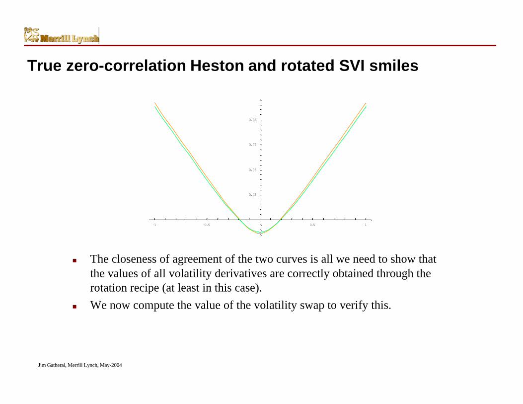
True zero-correlation Heston and rotated SVI smiles

n The closeness of agreement of the two curves is all we need to show thatthe values of all volatility derivatives are correctly obtained through therotation recipe (at least in this case).

n We now compute the value of the volatility swap to verify this.

-1 -0.5 0.5 1

0.05

0.06

0.07

0.08


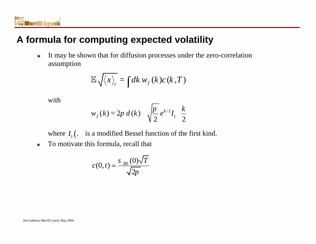
A formula for computing expected volatility

n It may be shown that for diffusion processes under the zero-correlationassumption

with/ 2

1( ) 2 ( )2 2

kf

kw k k e Iππ δ = +

( ) ( , )ftx dk w k c k T= ∫E

where is a modified Bessel function of the first kind.n To motivate this formula, recall that

( )1 .I

(0)(0, )

2BS T

c tσ

π;


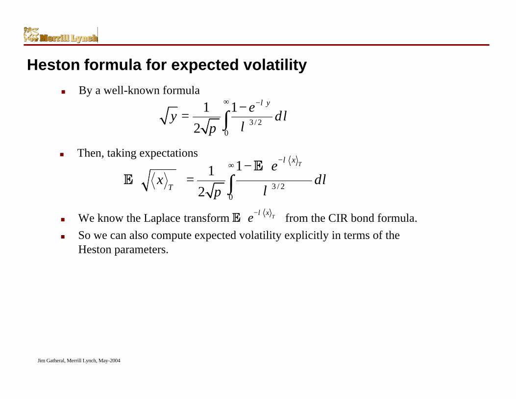
Heston formula for expected volatility

n By a well-known formula

n Then, taking expectations

3 / 20

1 12

yey d

λ

λλπ

∞ −−= ∫

n We know the Laplace transform from the CIR bond formula.n So we can also compute expected volatility explicitly in terms of the

Heston parameters.

3 / 20

112

Tx

T

ex d

λ

λλπ

−∞ − = ∫

EET

xe λ− E


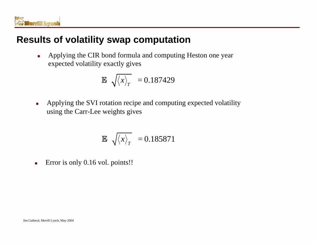
Results of volatility swap computation

n Applying the CIR bond formula and computing Heston one yearexpected volatility exactly gives

0.187429T

x = E

n Applying the SVI rotation recipe and computing expected volatilityusing the Carr-Lee weights gives

0.185871T

x = E

n Error is only 0.16 vol. points!!


Summary

n Motivated by the asymptotic behavior of the implied volatility smile atextreme strikes, we introduced a parameterization (SVI).

n We demonstrated that this parameterization not only fits SPX optionprices extremely well but that it fits option prices generated by manytheoretical models. These models include stochastic volatility and purejump models.

n By identifying the form of the implied volatility smile as SVI for theHeston model in the limit of infinite time to expiration, we were able tomap the SVI parameters to parameters of the Heston model (in thislimit).

n Noting that volatility derivatives (under a stochastic volatilityassumption) cannot depend on the correlation between underlyingreturns and volatility changes, we developed a recipe transforming agiven set of SVI parameters into their zero-correlation world equivalents.

n We then applied Carr-Lee to the option prices thus generated to valuevolatility derivatives.

n We demonstrated that in the particular case of Heston one year Europeanoptions with BCC parameters, agreement was very close.


Referencesn Bakshi, G., Cao C. and Chen Z. (1997). Empirical performance of alternative

option pricing models. Journal of Finance, 52, 2003-2049.n Carr, Peter and Lee, Roger (2003), Robust Replication of Volatility Derivatives,

Courant Institute, NYU and Stanford University.n Friz, Peter and Gatheral, J. (2004), Valuation of Volatility Derivatives as an

Inverse Problem, Merrill Lynch and Courant Institute, NYU.n Gatheral, J. (2003). Case studies in financial modeling lecture notes.

http://www.math.nyu.edu/fellows_fin_math/gatheral/case_studies.htmln Heston, Steven (1993). A closed-form solution for options with stochastic

volatility with applications to bond and currency options. The Review of FinancialStudies 6, 327-343.

n Hull, John and White Alan (1987), The pricing of options with stochasticvolatilities, The Journal of Finance 19, 281-300.

n Lee, Roger (2002). The Moment Formula for Implied Volatility at ExtremeStrikes. Forthcoming in Mathematical Finance.

n Lewis, Alan R. (2000), Option Valuation under Stochastic Volatility : withMathematica Code, Finance Press.

n Schoutens W., Simons E. and Tistaert J. (2004). A Perfect Calibration! NowWhat?, Wilmott Magazine, March, pages 66-78.

a parsimonious arbitrage-free implied volatility...

Documents