an introduction to analytica analytica 3.1 for windows
TRANSCRIPT
TutorialAn Introduction to Analytica
Analytica 3.1 for Windows

Copyright noticeInformation in this document is subject to change without notice and does not represent a commitment on the part of Lumina Decision Systems, Inc. The software program described in this document is provided under a license agreement. The software may be used or copied, and registration numbers transferred, only in accordance with the terms of the agreement. It is against the law to copy the software on any medium except as specifically allowed in the license agreement. No part of this document may be reproduced or transmitted in any form or by any means, electronic or mechanical, including photocopying, recording, or information storage and retrieval systems, for any purpose other than the licensee's personal use, without the express written consent of Lumina Decision Systems, Inc.
This document is 1993-2005 Lumina Decision Systems, Inc. All rights reserved.
The software program described in this document, Analytica, is copyrighted: 1982-1991 Carnegie Mellon University 1992-2005 Lumina Decision Systems, Inc., all rights reserved.
Analytica was written using MacApp: 1985-1996 Apple Computer, Inc.Analytica incorporates Mac2Win technology, (c) 1997 Altura Software, Inc.
The Analytica software contains software technology licensed from Carnegie Mellon University exclusively to Lumina Decision Systems, Inc., and includes software proprietary to Lumina Decision Systems, Inc. The MacApp software is proprietary to Apple Computer, Inc. The Mac2Win technology is technology to Altura, Inc. Both MacApp and Mac2Win are licensed to Lumina Decision Systems only for use in combination with the Analytica program. Neither Lumina nor its Licensors, Carnegie Mellon University, Apple Computer, Inc., and Altura Software, Inc., make any warranties whatsoever, either express or implied, regarding the Analytica product, including warranties with respect to its merchantability or its fitness for any particular purpose.
Analytica is a registered trademark of Lumina Decision Systems, Inc.
Lumina Decision Systems, Inc.26010 Highland WayLos Gatos, CA 95033Phone: 650-212-1212 Fax: 650-240-2230Web Site: www.lumina.com
Contents
Introduction: About AnalyticaWelcome to Analytica.................................................................. 3Who can use Analytica................................................................ 4Tutorial overview ......................................................................... 4Installing Analytica ...................................................................... 6Conventions used in this tutorial ................................................. 6Assumed background ................................................................. 8Chapter 1: Using the Rent vs. Buy ModelOpening the Rent vs. Buy model .............................................. 11Becoming familiar with the diagram window ............................. 12Using Online Help ..................................................................... 13Computing an output value ....................................................... 13Changing input values and recomputing................................... 16Examining and changing an uncertain input ............................. 18Displaying alternative uncertain views ...................................... 21Using the Rent vs. Buy model: Summary ................................. 25Saving your model .................................................................... 26Closing your model without saving............................................ 27Quitting Analytica ...................................................................... 28
Chapter 2: Exploring the Rent vs.Buy ModelRecognizing an influence diagram ............................................ 31Opening an Object window ....................................................... 33Moving between Object windows.............................................. 35Using the Attribute panel........................................................... 38Inspecting definitions in the Attribute panel............................... 39Opening a module..................................................................... 41Inspecting values in the Attribute panel .................................... 46Displaying results ...................................................................... 47Exploring the Rent vs. Buy model: Summary............................ 51
Chapter 3:Analyzing the Rent vs. Buy Analysis ModelExamining the difference between renting and buying ............. 55Importance analysis .................................................................. 57Performing parametric (sensitivity) analysis.............................. 60
Evaluating alternative decisions ......................................... 65Analyzing the Rent vs. Buy Analysis model: Summary............. 72
Chapter 4: Creating a ModelDocumenting the model ............................................................ 75Editing a diagram ...................................................................... 76
Analytica Tutorial i
4 Contents
Creating variables ......................................................................77Saving your model .....................................................................79Deleting a variable .....................................................................80Moving nodes.............................................................................81Editing variable titles ..................................................................83Drawing an arrow between nodes .............................................84Deleting an arrow.......................................................................85Connecting multiple arrows........................................................86Entering attributes using the Object window..............................88Defining a variable explicitly.......................................................90Defining a variable that is influenced by other variables ............93Probabilistic definition ................................................................96Entering attributes using the Attribute panel ..............................99Creating a module....................................................................102Drawing arrows between variables in different modules..........104Completing the model ..............................................................108Creating the Car Cost model: Summary ..................................111Saving your model and quitting................................................111Chapter 5: Creating Arrays (Tables)Creating an index variable .......................................................115Creating an array (table) ..........................................................117Selecting an array index ..........................................................119Creating another array using the same index ..........................120Viewing results of an array calculation.....................................123Combining results from a table ................................................131Adding a dimension to a variable .............................................132Completing the model ..............................................................135Creating Arrays (Tables): Summary.........................................136
Chapter 6: Creating the Party Problem ModelDocumenting the model ...........................................................140Creating the variables: Party Location, Weather, and Utility....141Drawing arrows between the variables ....................................142Defining Party Location as a list of labels ................................143Defining Weather as a probability table ...................................144Defining Utility as a deterministic table ....................................148Computing Utility ......................................................................151Creating the Party Problem model: Summary..........................154
Exercise.............................................................................154
Chapter 7: Creating the Foxes and Hares ModelDocumenting the model ...........................................................157Creating the Foxes and Hares diagram ...................................158
ii Analytica Tutorial
Contents
Defining Hare birth rate and Fox birth rate.............................. 159Defining the Time variable ...................................................... 160Defining hare population as a function of time ........................ 162Defining the fox population as a function of time .................... 167Creating the Populations objective.......................................... 168Defining the population control: foxes capture hares .............. 171Defining the population control: foxes require hares............... 178Viewing the final results of both populations ........................... 181Creating the Foxes and Hares Model: Summary .................... 182Chapter 8: On Your OwnBusiness Examples................................................................. 185
Bond Model....................................................................... 185Breakeven Analysis .......................................................... 186Expected R&D Project Value............................................ 186Financial Statement Templates ........................................ 186Market Model .................................................................... 186Plan_Schedule_Control .................................................... 187Sales Effectiveness .......................................................... 187Subscriber Pricing............................................................. 187
Decision Analysis .................................................................... 1882 Branch Party Tree.......................................................... 188Beta Updating ................................................................... 188Biotech R&D Portfolio ....................................................... 188Gibbs Sampling in Bayesian Network............................... 188LEV R&D Strategy ............................................................ 189Newton-Raphson Method ................................................. 189Nonsymmetric Tree .......................................................... 189Party With Forecast .......................................................... 189Supply and Demand ......................................................... 189Tornado Diagrams ............................................................ 189Upgrade Decision ............................................................. 191
Dynamic Models...................................................................... 191Leveling ............................................................................ 191Markov Chain.................................................................... 191Mass-Spring-Damper........................................................ 192Projectile Motion ............................................................... 192Unequal time steps ........................................................... 193
Engineering Examples ............................................................ 193Adaptive Filter................................................................... 193Antenna Gain.................................................................... 193Failure Analysis ................................................................ 193
Function Examples.................................................................. 193Autocorrelation.................................................................. 193
Analytica Tutorial iii
4 Contents
Choice and Determtable....................................................193Correlated Distributions .....................................................194Correlated Normals ...........................................................194DBWrite Example ..............................................................194Discrete Sampling .............................................................194Extracting Diagonal ...........................................................194Regression Examples........................................................194Sorting People by Height...................................................194Subset of Array..................................................................195Swapping y and x-index ....................................................195Use of MDTable.................................................................195Risk Analysis............................................................................195Seat belt safety..................................................................195Txc.....................................................................................196
Libraries ...................................................................................196Bayes function ...................................................................196Continuous Distributions....................................................197Data Statistics Library........................................................197Discrete Distributions.........................................................197Expand Index.....................................................................197Financial Library ................................................................197ODBC-Library ....................................................................198
User Guide Examples ..............................................................198Analyzing Unc & Sens .......................................................198Array Examples .................................................................198Array Function Examples ..................................................198Continuous Distributions....................................................198Discrete Distributions.........................................................199Dynamic & Dependencies .................................................199Dynamic & Uncertainty ......................................................199Dynamic Example 1...........................................................199Dynamic Example 2...........................................................199Expression Examples ........................................................199Input and Output Nodes ....................................................199
Summary..................................................................................200
GlossaryCredits
Analytica Windows and DialogsAnalytica Quick Reference
The Tool Bar......................................................................214Numerical Formats (Output) ..............................................214Numerical Prefixes and Suffixes (Input) ............................214
iv Analytica Tutorial

Introduction
About Analytica

In this Chapter
This introduction tells you how to use this manual.
Introduction: About AnalyticaWelcome to Analytica
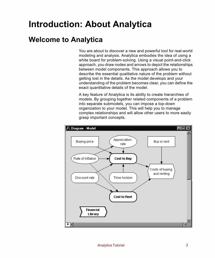
You are about to discover a new and powerful tool for real-world modeling and analysis. Analytica embodies the idea of using a white board for problem-solving. Using a visual point-and-click approach, you draw nodes and arrows to depict the relationships between model components. This approach allows you to describe the essential qualitative nature of the problem without getting lost in the details. As the model develops and your understanding of the problem becomes clear, you can define the exact quantitative details of the model.
A key feature of Analytica is its ability to create hierarchies of models. By grouping together related components of a problem into separate submodels, you can impose a top-down organization to your model. This will help you to manage complex relationships and will allow other users to more easily grasp important concepts.
Analytica Tutorial 3
Chapter Who can use AnalyticaI
Another key feature of Analytica is the use of Intelligent Arrays™. These enable you to add or remove dimensions such as time periods, geographic regions, alternative decisions, etc., with minimal changes to the model structure. Unlike spreadsheets, which require you to repeat formulas with each new dimension, Analytica separates the dimensions from the relationships so that models remain simple. As the dimensions change, Analytica automatically updates, reports, and graphs the results.Each node in an Analytica model has a window that displays the node’s inputs and outputs, and allows you to enter definitions, descriptions, units of measure, and other documentary information. This self-documenting capability, combined with hierarchical models and Intelligent Arrays™, makes it easier to understand and communicate how models work.
Analytica also features fully integrated risk and sensitivity analysis for analyzing models with uncertain inputs; powerful facilities for time-dependent, dynamic simulations; comprehensive overlay graphs; and over 100 financial, statistical, and scientific functions for calculating just about any type of mathematical expression.
Who can use AnalyticaAnalytica is for the modeler and problem solver—from the financial analyst modeling business opportunities to the engineer designing new products to the scientist investigating the behavior of physical phenomena.
It is particularly suited to users in the fields of management consulting, health and environmental sciences, aerospace, oil & gas, construction, manufacturing, financial services, and investing.
Tutorial overviewThis tutorial is a hands-on introduction to using Analytica. Step-by-step instructions show you how to explore and analyze an existing Analytica model and how to create a new Analytica model. Because later tutorial sections build on the material in earlier chapters, you should work through the chapters in sequence.
We recommend that everyone new to Analytica complete Chapters 1 through 5, which will take two to three hours. If you want to work more quickly, skip the text and only follow the
4 Analytica Tutorial
Chapter Tutorial overviewI
instructions in the boxed steps. Then, if you are unsure about any terms or concepts, look them up in the glossary, or review the text.This tutorial is designed to introduce you to some of Analytica’s basic features. Once you are familiar with the basics, refer to the Analytica User Guide for more detailed information on Analytica's features.
• Chapter 1 – Using the Rent vs. Buy Model
This chapter shows how to open an Analytica model. Using a simple interface to an example model that analyzes the total costs of buying or renting a house, you will calculate results and change input values to see the effects on the results. You will display uncertain results in a variety of ways.
• Chapter 2 – Exploring the Rent vs. Buy Model
This chapter shows you how to browse a model’s structure and assumptions by examining its influence diagrams, variables, and definitions.
• Chapter 3 – Analyzing the Rent vs. Buy Analysis Model
This chapter shows you how to perform importance analysis and sensitivity analysis to see which uncertain variables most heavily influence the outcome.
• Chapter 4 – Creating a Model
This chapter shows you how to create a new Analytica model. In the process of building a model that analyzes the costs of owning and operating an automobile, you will create variables, define relationships between variables, add documentary text, and compute results. In addition, you will create modules and add dependencies between modules.
• Chapter 5 – Creating Arrays (Tables)
This chapter shows you how to add index variables and Edit Tables to a model, and demonstrates how tables work in Analytica, including an introduction to table functions.
• Chapter 6 – Creating the Party Problem Model
This chapter walks you through a familiar problem: where to have your next party. This model introduces probability tables and conditional deterministic tables. You should complete this chapter if your models will use discrete or conditional uncertainties.
Analytica Tutorial 5
Chapter Installing AnalyticaI
• Chapter 7 – Creating the Foxes and Hares ModelIn this chapter you create a dynamic model of population sizes that depend on each other and that change with time. You should complete this chapter if your models will use dynamic simulation or variables that change over time.
• Chapter 8 – On Your Own
This chapter briefly describes all the example models provided with Analytica. You should investigate these as you begin to build your own models.
Installing AnalyticaBefore you start this tutorial, follow these steps to install the Analytica application and associated model files on your hard disk:
1. Start Windows.
2. Insert the Analytica CD in your computer’s CD-ROM drive.
3. The Windows Installer should automatically start up and begin installing Analytica
If the AutoRun function does not work, follow these alternate steps:
3. Click on the Start button on the Windows taskbar.
4. Select Run from the popup menu.
5. In the Run dialog box, specify the program SETUP.EXE on your CD-ROM drive (usually either the D: or E: drive).
6. Click on OK.
The setup program requires some responses from you. For example, you will be asked to verify the directory name in which Analytica will be installed. Most users can accept the defaults provided by the setup program. The default installation location for Analytica is C:\Program Files\Lumina\Analytica 3.1.
Conventions used in this tutorialThe conventions used in this tutorial are as follows:
• Boxed, numbered instructions along the left side of the page give you the steps to take.
6 Analytica Tutorial
Chapter Conventions used in this tutorialI
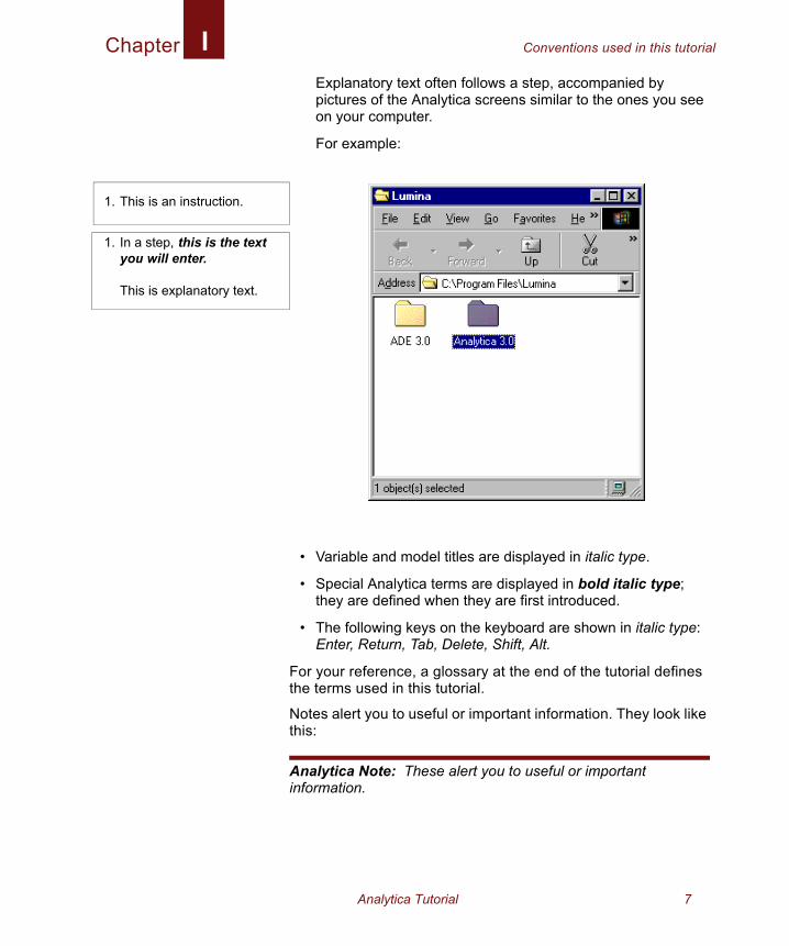
Explanatory text often follows a step, accompanied by pictures of the Analytica screens similar to the ones you see on your computer.For example:
• Variable and model titles are displayed in italic type.
• Special Analytica terms are displayed in bold italic type; they are defined when they are first introduced.
• The following keys on the keyboard are shown in italic type: Enter, Return, Tab, Delete, Shift, Alt.
For your reference, a glossary at the end of the tutorial defines the terms used in this tutorial.
Notes alert you to useful or important information. They look like this:
Analytica Note: These alert you to useful or important information.
1. This is an instruction.
1. In a step, this is the text you will enter.
This is explanatory text.
Analytica Tutorial 7
Chapter Assumed backgroundI
Assumed backgroundThis tutorial assumes that you already have the basic skills needed to run Windows programs, including the following:
You also need to know how to use pulldown and popup menus, scroll bars, and windows.
If you are not familiar with these basic operations, look at the reference material that came with your computer.
This tutorial also assumes that you have basic skills of financial or quantitative modeling—for example, from previously using a spreadsheet program.
It assumes that you are acquainted with elementary statistics and are comfortable with the concepts of mean, median, and standard deviation. It also assumes that you have some understanding of probability distributions, such as the normal and uniform, and are familiar with the concepts of probability density function and cumulative distribution function. These terms are reviewed briefly in the Glossary at the end of the tutorial.
Term Meaningclick Press and release the mouse button one time.
double-click Press and release the mouse button two times.
drag Press and hold down the mouse button while moving the cursor to a new location on the screen, then release the mouse button.
press Press and hold down the mouse button.
select Click on an interface object, such as a menu command or a cell in a table; selected objects usually appear highlighted.
8 Analytica Tutorial
Chapter 1
Using the Rent vs. Buy Model

In this Chapter
This chapter shows you how to:
• Open an existing model
• Calculate results
• Change input values to calculate different results
Chapter 1: Using the Rent vs. Buy ModelIn this chapter, you use the Rent vs. Buy model, an Analytica™ model that compares the cost of renting a house to the cost of buying one. After working through the chapter, you will know how to open an existing model, use it to calculate results, and change input values to calculate different results.
Opening the Rent vs. Buy model
To begin, follow these steps.
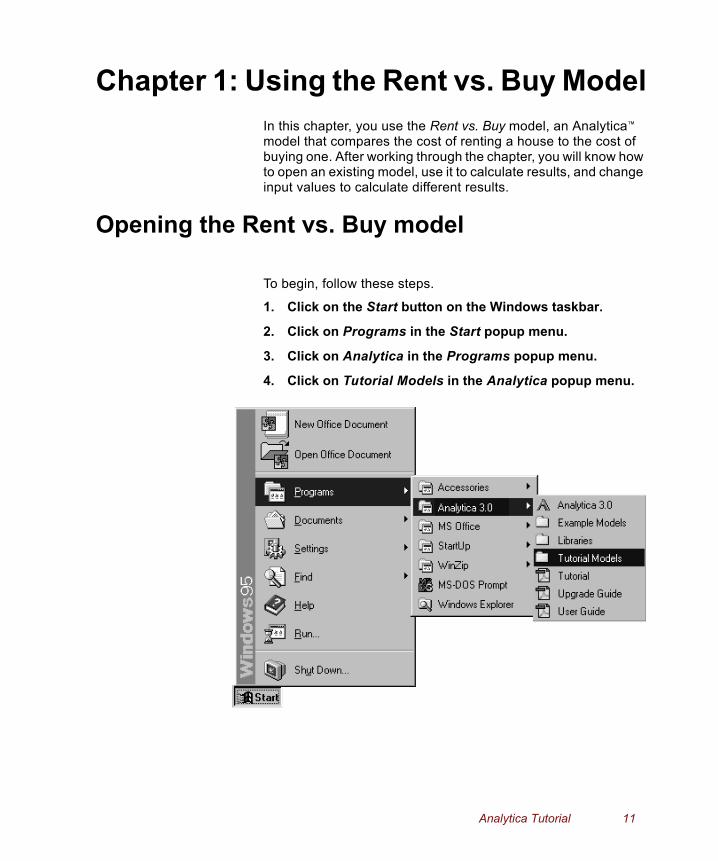
1. Click on the Start button on the Windows taskbar.
2. Click on Programs in the Start popup menu.
3. Click on Analytica in the Programs popup menu.
4. Click on Tutorial Models in the Analytica popup menu.
Analytica Tutorial 11
Chapter Becoming familiar with the diagram window1
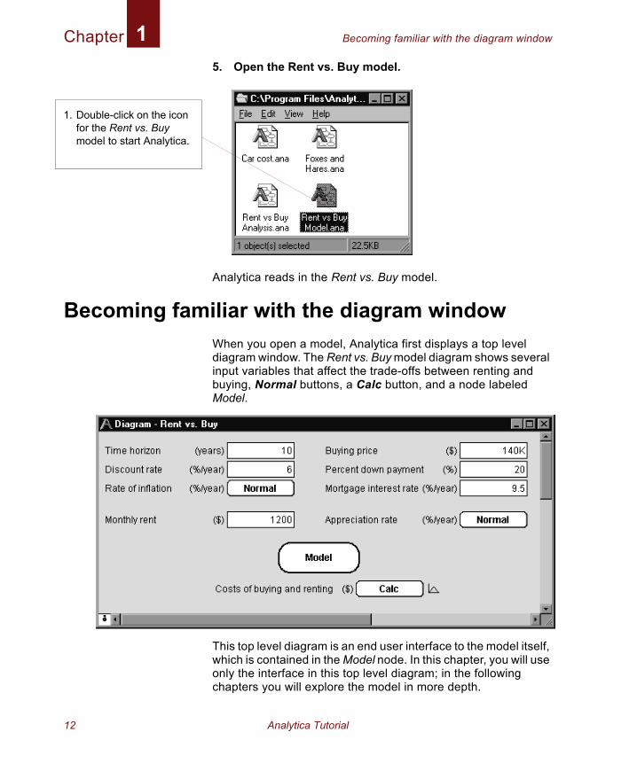
5. Open the Rent vs. Buy model.Analytica reads in the Rent vs. Buy model.
Becoming familiar with the diagram windowWhen you open a model, Analytica first displays a top level diagram window. The Rent vs. Buy model diagram shows several input variables that affect the trade-offs between renting and buying, Normal buttons, a Calc button, and a node labeled Model.
This top level diagram is an end user interface to the model itself, which is contained in the Model node. In this chapter, you will use only the interface in this top level diagram; in the following chapters you will explore the model in more depth.
1. Double-click on the icon for the Rent vs. Buy model to start Analytica.
12 Analytica Tutorial
Chapter Using Online Help1
1
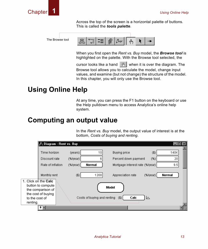
Across the top of the screen is a horizontal palette of buttons. This is called the tools palette.
When you first open the Rent vs. Buy model, the Browse tool is highlighted on the palette. With the Browse tool selected, the
cursor looks like a hand when it is over the diagram. The Browse tool allows you to calculate the model, change input values, and examine (but not change) the structure of the model. In this chapter, you will only use the Browse tool.
Using Online HelpAt any time, you can press the F1 button on the keyboard or use the Help pulldown menu to access Analytica’s online help system.
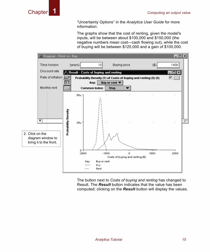
Computing an output valueIn the Rent vs. Buy model, the output value of interest is at the bottom, Costs of buying and renting.
The Browse tool
. Click on the Calc button to compute the comparison of the cost of buying to the cost of renting.
Analytica Tutorial 13
Chapter Computing an output value1
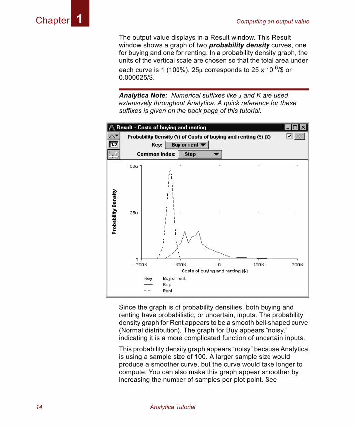
The output value displays in a Result window. This Result window shows a graph of two probability density curves, one for buying and one for renting. In a probability density graph, the units of the vertical scale are chosen so that the total area under each curve is 1 (100%). 25µ corresponds to 25 x 10-6/$ or 0.000025/$.Analytica Note: Numerical suffixes like µ and K are used extensively throughout Analytica. A quick reference for these suffixes is given on the back page of this tutorial.
Since the graph is of probability densities, both buying and renting have probabilistic, or uncertain, inputs. The probability density graph for Rent appears to be a smooth bell-shaped curve (Normal distribution). The graph for Buy appears “noisy,” indicating it is a more complicated function of uncertain inputs.
This probability density graph appears “noisy” because Analytica is using a sample size of 100. A larger sample size would produce a smoother curve, but the curve would take longer to compute. You can also make this graph appear smoother by increasing the number of samples per plot point. See
14 Analytica Tutorial
Chapter Computing an output value1
2
“Uncertainty Options” in the Analytica User Guide for more information.
The graphs show that the cost of renting, given the model's inputs, will be between about $100,000 and $150,000 (the negative numbers mean cost—cash flowing out), while the cost of buying will be between $125,000 and a gain of $100,000.
The button next to Costs of buying and renting has changed to Result. The Result button indicates that the value has been computed; clicking on the Result button will display the values.
. Click on the diagram window to bring it to the front.
Analytica Tutorial 15
Chapter Changing input values and recomputing1
1.
2
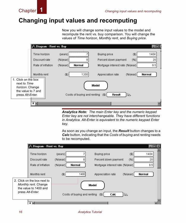
Changing input values and recomputingNow you will change some input values to the model and recompute the rent vs. buy comparison. You will change the values of Time horizon, Monthly rent, and Buying price.
Analytica Note: The main Enter key and the numeric keypad Enter key are not interchangeable. They have different functions in Analytica. Alt-Enter is equivalent to the numeric keypad Enter key.
As soon as you change an input, the Result button changes to a Calc button, indicating that the Costs of buying and renting needs to be recomputed.
Click on the box next to Time horizon. Change the value to 7 and press Alt-Enter.
. Click on the box next to Monthly rent. Change the value to 1400 and press Alt-Enter.
16 Analytica Tutorial
Chapter Changing input values and recomputing1
4
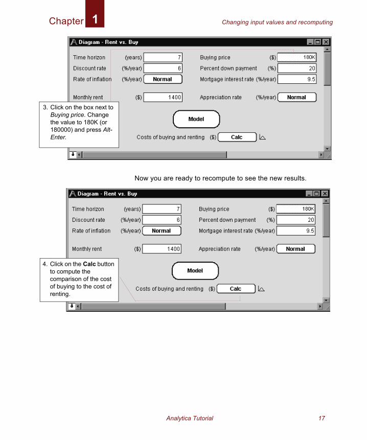
Now you are ready to recompute to see the new results.
3. Click on the box next to Buying price. Change the value to 180K (or 180000) and press Alt-Enter.
. Click on the Calc button to compute the comparison of the cost of buying to the cost of renting.
Analytica Tutorial 17
Chapter Examining and changing an uncertain input1
5
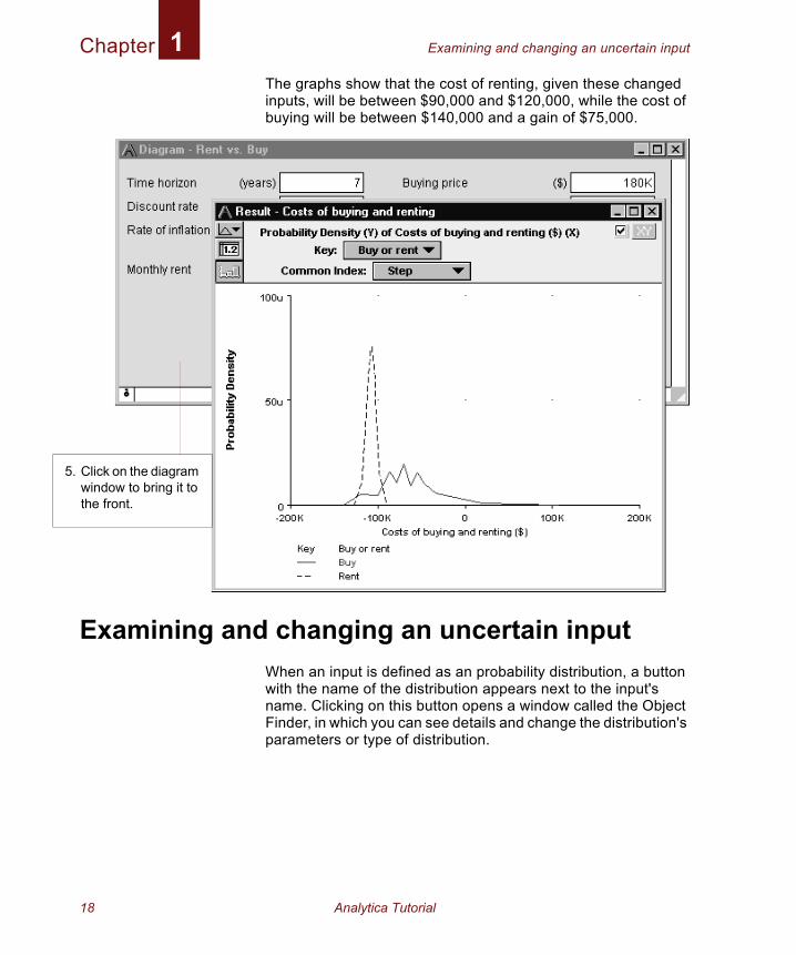
The graphs show that the cost of renting, given these changed inputs, will be between $90,000 and $120,000, while the cost of buying will be between $140,000 and a gain of $75,000.
Examining and changing an uncertain inputWhen an input is defined as an probability distribution, a button with the name of the distribution appears next to the input's name. Clicking on this button opens a window called the Object Finder, in which you can see details and change the distribution's parameters or type of distribution.
. Click on the diagram window to bring it to the front.
18 Analytica Tutorial
Chapter Examining and changing an uncertain input1
1.
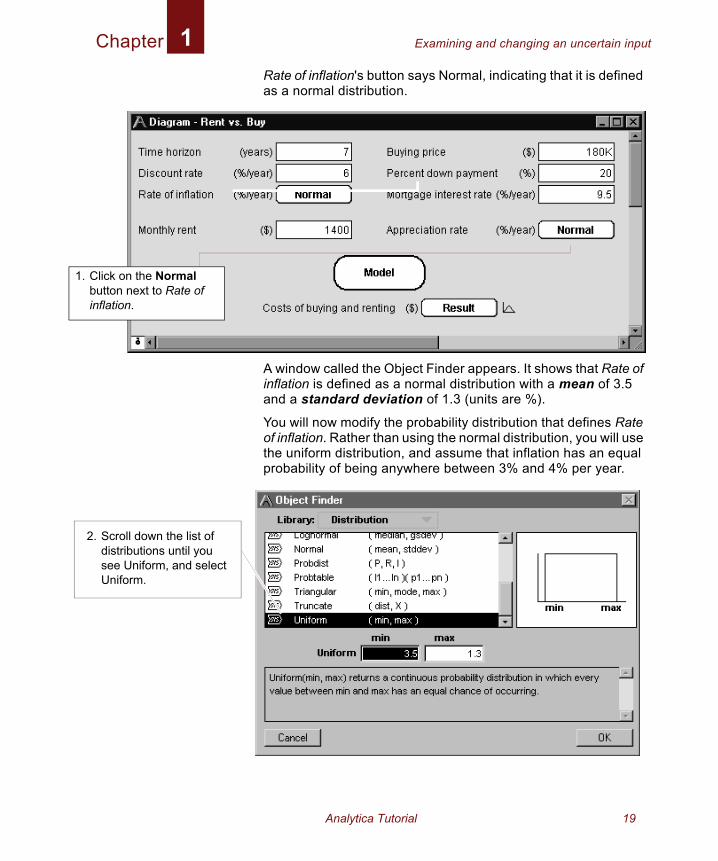
Rate of inflation's button says Normal, indicating that it is defined as a normal distribution.
A window called the Object Finder appears. It shows that Rate of inflation is defined as a normal distribution with a mean of 3.5 and a standard deviation of 1.3 (units are %).
You will now modify the probability distribution that defines Rate of inflation. Rather than using the normal distribution, you will use the uniform distribution, and assume that inflation has an equal probability of being anywhere between 3% and 4% per year.
Click on the Normal button next to Rate of inflation.
2. Scroll down the list of distributions until you see Uniform, and select Uniform.
Analytica Tutorial 19
Chapter Examining and changing an uncertain input1
5. Ctocoore
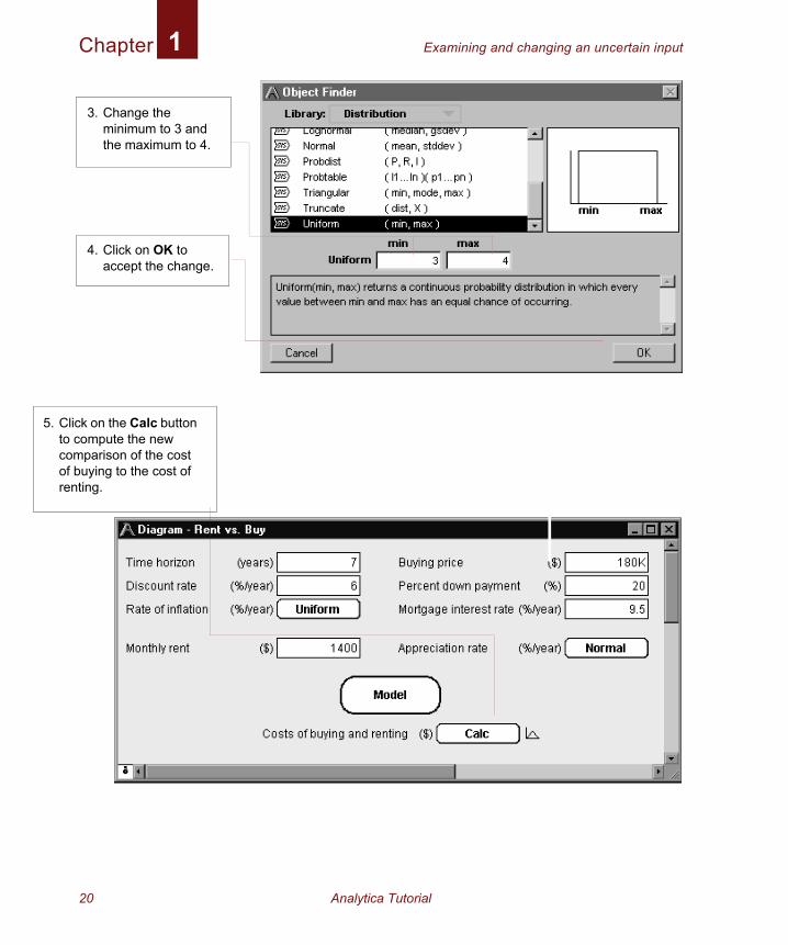
3. Change the minimum to 3 and the maximum to 4.
4. Click on OK to accept the change.
lick on the Calc button compute the new mparison of the cost
f buying to the cost of nting.
20 Analytica Tutorial
Chapter Displaying alternative uncertain views1
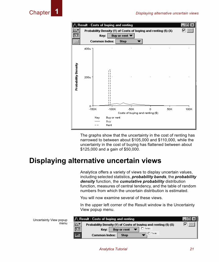
The graphs show that the uncertainty in the cost of renting has narrowed to between about $105,000 and $110,000, while the uncertainty in the cost of buying has flattened between about $125,000 and a gain of $50,000.
Displaying alternative uncertain viewsAnalytica offers a variety of views to display uncertain values, including selected statistics, probability bands, the probability density function, the cumulative probability distribution function, measures of central tendency, and the table of random numbers from which the uncertain distribution is estimated.
You will now examine several of these views.
In the upper left corner of the Result window is the Uncertainty View popup menu.
Uncertainty View popupmenu
Analytica Tutorial 21
Chapter Displaying alternative uncertain views1
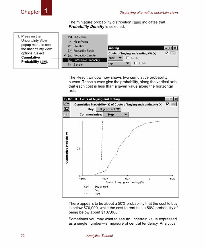
The miniature probability distribution [ ] indicates that Probability Density is selected.The Result window now shows two cumulative probability curves. These curves give the probability, along the vertical axis, that each cost is less than a given value along the horizontal axis.
There appears to be about a 50% probability that the cost to buy is below $70,000, while the cost to rent has a 50% probability of being below about $107,000.
Sometimes you may want to see an uncertain value expressed as a single number—a measure of central tendency. Analytica
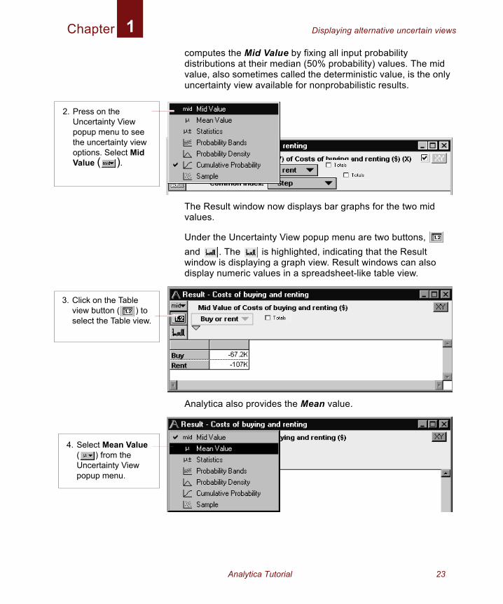
1. Press on the Uncertainty View popup menu to see the uncertainty view options. Select Cumulative Probability ( ).
22 Analytica Tutorial
Chapter Displaying alternative uncertain views1
computes the Mid Value by fixing all input probability distributions at their median (50% probability) values. The mid value, also sometimes called the deterministic value, is the only uncertainty view available for nonprobabilistic results.The Result window now displays bar graphs for the two mid values.
Under the Uncertainty View popup menu are two buttons, and . The is highlighted, indicating that the Result window is displaying a graph view. Result windows can also display numeric values in a spreadsheet-like table view.
Analytica also provides the Mean value.
2. Press on the Uncertainty View popup menu to see the uncertainty view options. Select Mid Value ( ).
3. Click on the Table view button ( ) to select the Table view.
4. Select Mean Value ( ) from the Uncertainty View popup menu.
Analytica Tutorial 23
Chapter Displaying alternative uncertain views1
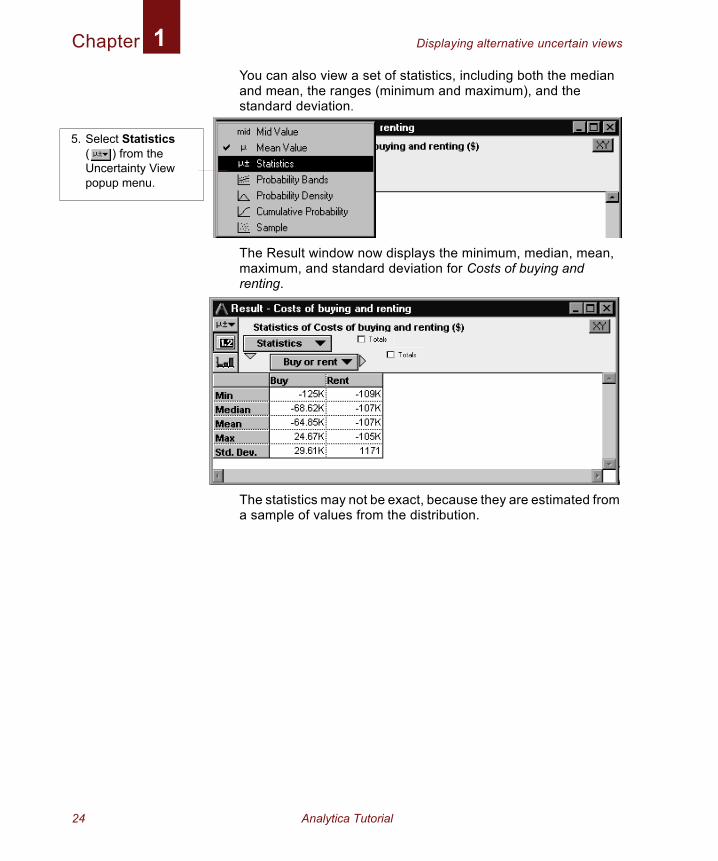
You can also view a set of statistics, including both the median and mean, the ranges (minimum and maximum), and the standard deviation.The Result window now displays the minimum, median, mean, maximum, and standard deviation for Costs of buying and renting.
The statistics may not be exact, because they are estimated from a sample of values from the distribution.
5. Select Statistics ( ) from the Uncertainty View popup menu.
24 Analytica Tutorial
Chapter Using the Rent vs. Buy model: Summary1
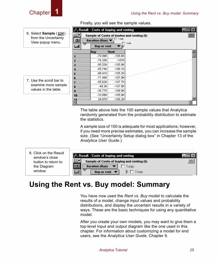
Finally, you will see the sample values.The table above lists the 100 sample values that Analytica randomly generated from the probability distribution to estimate the statistics.
A sample size of 100 is adequate for most applications; however, if you need more precise estimates, you can increase the sample size. (See “Uncertainty Setup dialog box” in Chapter 13 of the Analytica User Guide.)
Using the Rent vs. Buy model: SummaryYou have now used the Rent vs. Buy model to calculate the results of a model, change input values and probability distributions, and display the uncertain results in a variety of ways. These are the basic techniques for using any quantitative model.
After you create your own models, you may want to give them a top-level input and output diagram like the one used in this chapter. For information about customizing a model for end users, see the Analytica User Guide, Chapter 9.
6. Select Sample ( ) from the Uncertainty View popup menu.
7. Use the scroll bar to examine more sample values in the table.
8. Click on the Result window’s close button to return to the Diagram window.
Analytica Tutorial 25
Chapter Saving your model1
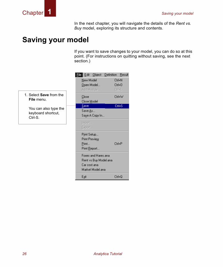
In the next chapter, you will navigate the details of the Rent vs. Buy model, exploring its structure and contents.Saving your modelIf you want to save changes to your model, you can do so at this point. (For instructions on quitting without saving, see the next section.)
1. Select Save from the File menu.
You can also type the keyboard shortcut, Ctrl-S.
26 Analytica Tutorial
Chapter Closing your model without saving1
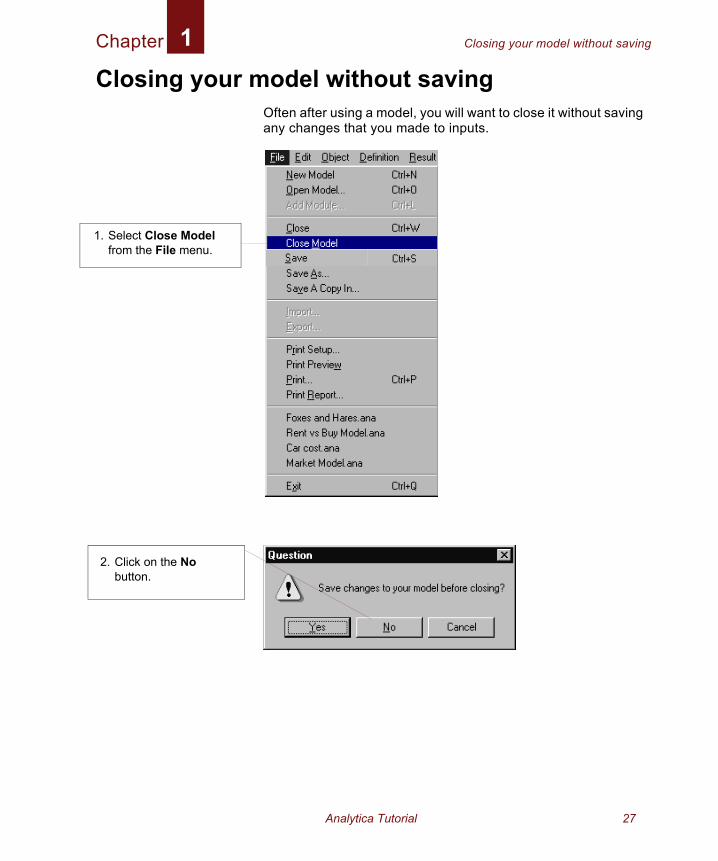
Closing your model without savingOften after using a model, you will want to close it without saving any changes that you made to inputs.
1. Select Close Model from the File menu.
2. Click on the No button.
Analytica Tutorial 27
Chapter Quitting Analytica1
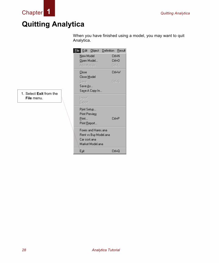
Quitting AnalyticaWhen you have finished using a model, you may want to quit Analytica.
1. Select Exit from the File menu.
28 Analytica Tutorial
Chapter 2
Exploring the Rent vs. Buy Model

In this Chapter
This chapter shows you how to explore a model by examining its:
• Influence diagrams
• Variables
• Attributes
• Definitions
• Results
1. DM
Chapter 2: Exploring the Rent vs.Buy ModelThis chapter assumes you have started Analytica and have opened the Rent vs. Buy model. If this is not the case, see “Opening the Rent vs. Buy model” on page 11.
In this chapter, you will examine the structure and contents of the Rent vs. Buy model.
The Rent vs. Buy model uses financial flow conventions: funds flowing in (received) have positive values; funds flowing out (expended) have negative values.
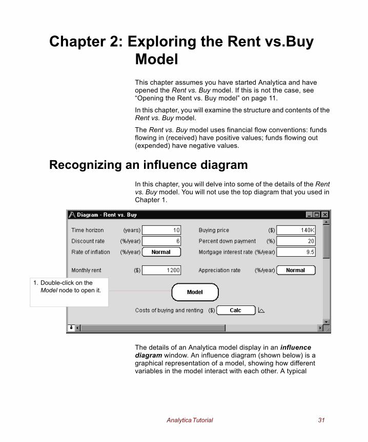
Recognizing an influence diagramIn this chapter, you will delve into some of the details of the Rent vs. Buy model. You will not use the top diagram that you used in Chapter 1.
The details of an Analytica model display in an influence diagram window. An influence diagram (shown below) is a graphical representation of a model, showing how different variables in the model interact with each other. A typical
ouble-click on the odel node to open it.
Analytica Tutorial 31
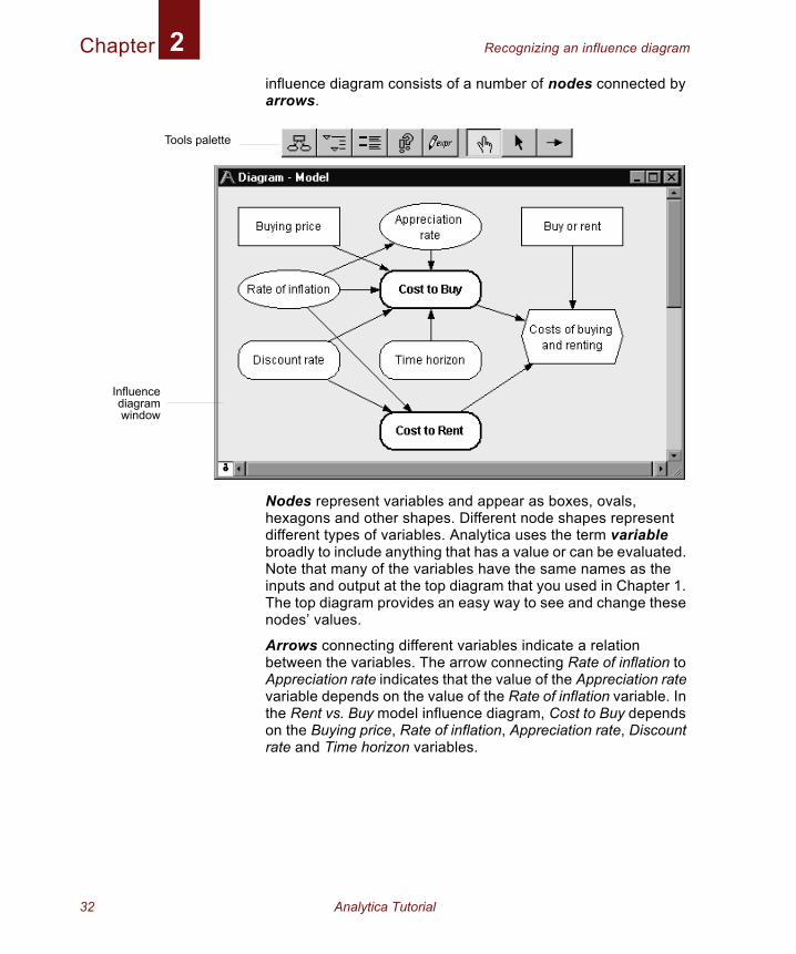
Chapter Recognizing an influence diagram2
influence diagram consists of a number of nodes connected by arrows.Nodes represent variables and appear as boxes, ovals, hexagons and other shapes. Different node shapes represent different types of variables. Analytica uses the term variable broadly to include anything that has a value or can be evaluated. Note that many of the variables have the same names as the inputs and output at the top diagram that you used in Chapter 1. The top diagram provides an easy way to see and change these nodes’ values.
Arrows connecting different variables indicate a relation between the variables. The arrow connecting Rate of inflation to Appreciation rate indicates that the value of the Appreciation rate variable depends on the value of the Rate of inflation variable. In the Rent vs. Buy model influence diagram, Cost to Buy depends on the Buying price, Rate of inflation, Appreciation rate, Discount rate and Time horizon variables.
Tools palette
Influencediagramwindow
32 Analytica Tutorial
Chapter Opening an Object window2
A De
A Ddirectl
of t
A Crepr
controdec
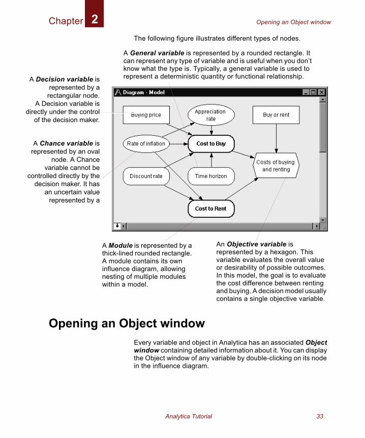
The following figure illustrates different types of nodes.
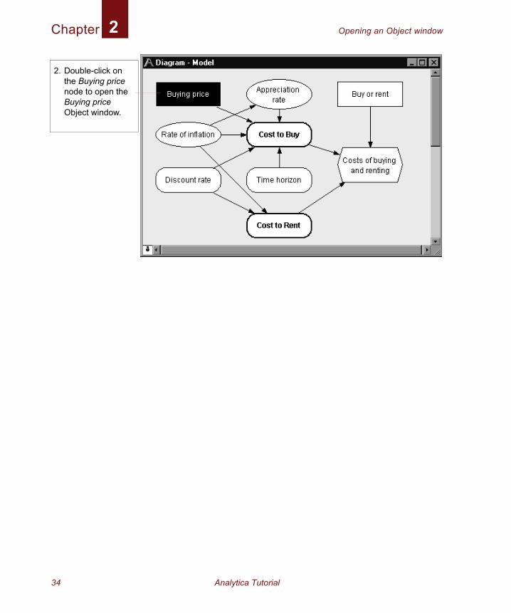
Opening an Object windowEvery variable and object in Analytica has an associated Object window containing detailed information about it. You can display the Object window of any variable by double-clicking on its node in the influence diagram.
cision variable isrepresented by arectangular node.ecision variable is
y under the controlhe decision maker.
hance variable isesented by an oval
node. A Chancevariable cannot belled directly by theision maker. It hasan uncertain value
represented by a
A Module is represented by a thick-lined rounded rectangle. A module contains its own influence diagram, allowing nesting of multiple modules within a model.
An Objective variable is represented by a hexagon. This variable evaluates the overall value or desirability of possible outcomes. In this model, the goal is to evaluate the cost difference between renting and buying. A decision model usually contains a single objective variable.
A General variable is represented by a rounded rectangle. It can represent any type of variable and is useful when you don’t know what the type is. Typically, a general variable is used to represent a deterministic quantity or functional relationship.
Analytica Tutorial 33
Chapter Opening an Object window2
2. Double-click on the Buying price node to open the Buying price Object window.
34 Analytica Tutorial
Chapter Moving between Object windows2
This
desthe v
The ti
provid
(unlim
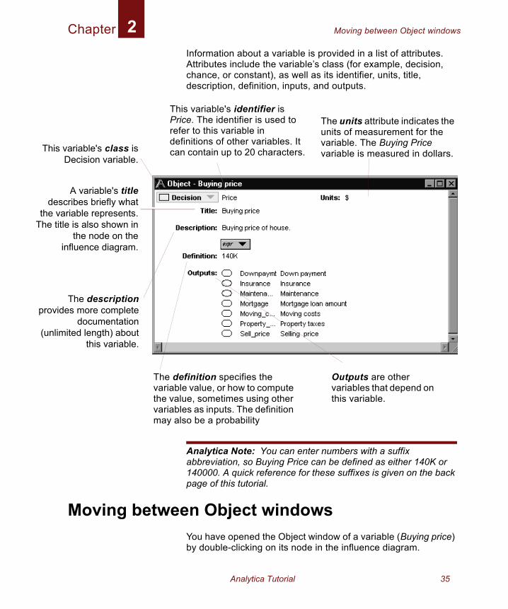
Information about a variable is provided in a list of attributes. Attributes include the variable’s class (for example, decision, chance, or constant), as well as its identifier, units, title, description, definition, inputs, and outputs.
Analytica Note: You can enter numbers with a suffix abbreviation, so Buying Price can be defined as either 140K or 140000. A quick reference for these suffixes is given on the back page of this tutorial.
Moving between Object windowsYou have opened the Object window of a variable (Buying price) by double-clicking on its node in the influence diagram.
This variable's identifier is Price. The identifier is used to refer to this variable in definitions of other variables. It can contain up to 20 characters.
The units attribute indicates the units of measurement for the variable. The Buying Price variable is measured in dollars. variable's class is
Decision variable.
A variable's titlecribes briefly what
ariable represents.tle is also shown in
the node on theinfluence diagram.
The descriptiones more complete
documentationited length) about
this variable.
The definition specifies the variable value, or how to compute the value, sometimes using other variables as inputs. The definition may also be a probability
Outputs are other variables that depend on this variable.
Analytica Tutorial 35
Chapter Moving between Object windows2
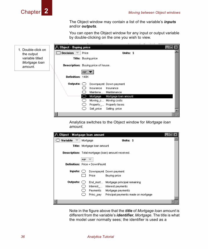
The Object window may contain a list of the variable’s inputs and/or outputs.You can open the Object window for any input or output variable by double-clicking on the one you wish to view.
Analytica switches to the Object window for Mortgage loan amount.
Note in the figure above that the title of Mortgage loan amount is different from the variable’s identifier, Mortgage. The title is what the model user normally sees; the identifier is used as a
1. Double-click on the output variable titled Mortgage loan amount.
36 Analytica Tutorial
Chapter Moving between Object windows2
2
mathematical symbol in the definitions of other variables that depend on this variable.
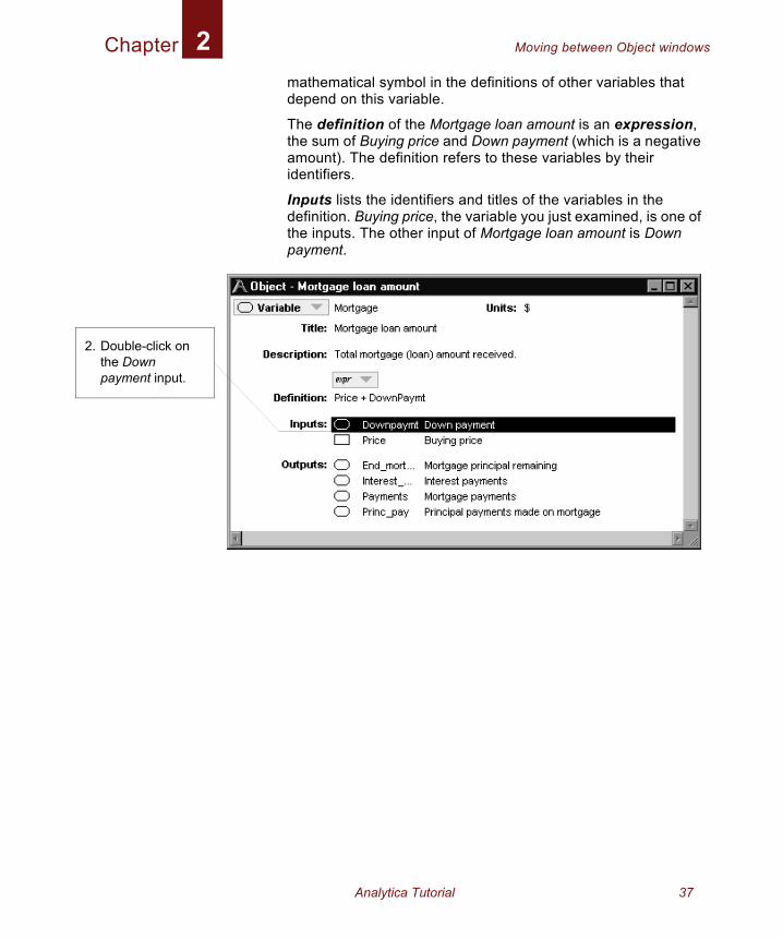
The definition of the Mortgage loan amount is an expression, the sum of Buying price and Down payment (which is a negative amount). The definition refers to these variables by their identifiers.
Inputs lists the identifiers and titles of the variables in the definition. Buying price, the variable you just examined, is one of the inputs. The other input of Mortgage loan amount is Down payment.
. Double-click on the Down payment input.
Analytica Tutorial 37
Chapter Using the Attribute panel2
3
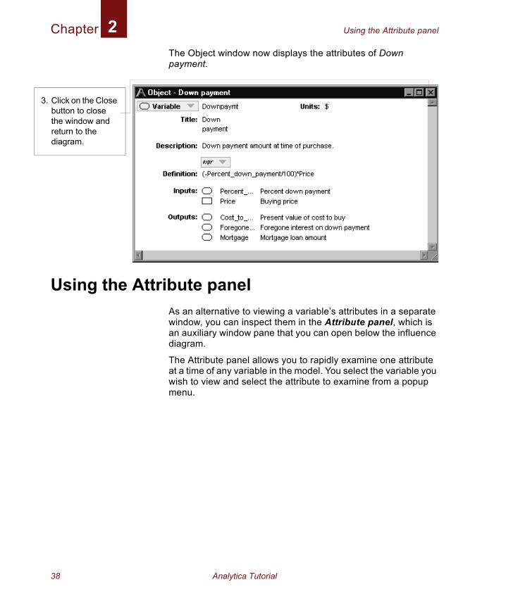
The Object window now displays the attributes of Down payment.
Using the Attribute panelAs an alternative to viewing a variable’s attributes in a separate window, you can inspect them in the Attribute panel, which is an auxiliary window pane that you can open below the influence diagram.
The Attribute panel allows you to rapidly examine one attribute at a time of any variable in the model. You select the variable you wish to view and select the attribute to examine from a popup menu.
. Click on the Close button to close the window and return to the diagram.
38 Analytica Tutorial
Chapter Inspecting definitions in the Attribute panel2
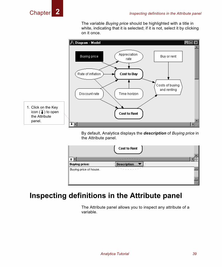
The variable Buying price should be highlighted with a title in white, indicating that it is selected; if it is not, select it by clicking on it once.By default, Analytica displays the description of Buying price in the Attribute panel.
Inspecting definitions in the Attribute panelThe Attribute panel allows you to inspect any attribute of a variable.
1. Click on the Key icon ( ) to open the Attribute panel.
Analytica Tutorial 39
Chapter Inspecting definitions in the Attribute panel2
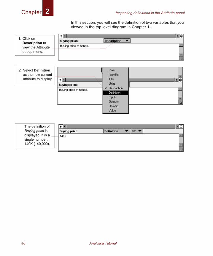
In this section, you will see the definition of two variables that you viewed in the top level diagram in Chapter 1.1. Click on Description to view the Attribute popup menu.
2. Select Definition as the new current attribute to display.
The definition of Buying price is displayed. It is a single number: 140K (140,000).
40 Analytica Tutorial
Chapter Opening a module2
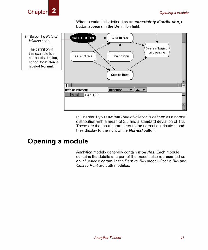
When a variable is defined as an uncertainty distribution, a button appears in the Definition field.In Chapter 1 you saw that Rate of inflation is defined as a normal distribution with a mean of 3.5 and a standard deviation of 1.3. These are the input parameters to the normal distribution, and they display to the right of the Normal button.
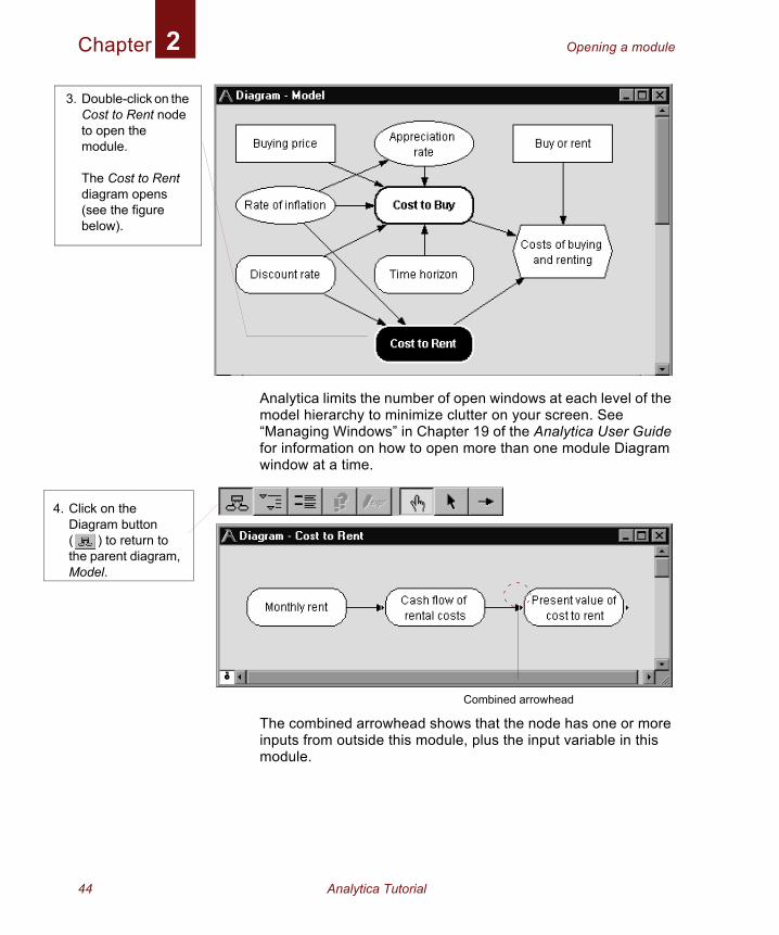
Opening a moduleAnalytica models generally contain modules. Each module contains the details of a part of the model, also represented as an influence diagram. In the Rent vs. Buy model, Cost to Buy and Cost to Rent are both modules.
3. Select the Rate of inflation node.
The definition in this example is a normal distribution; hence, the button is labeled Normal.
Analytica Tutorial 41
Chapter Opening a module2
1
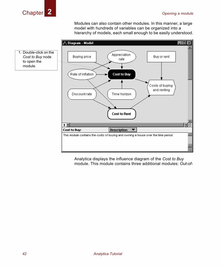
Modules can also contain other modules. In this manner, a large model with hundreds of variables can be organized into a hierarchy of models, each small enough to be easily understood.
Analytica displays the influence diagram of the Cost to Buy module. This module contains three additional modules: Out-of-
. Double-click on the Cost to Buy node to open the module.
42 Analytica Tutorial
Chapter Opening a module2
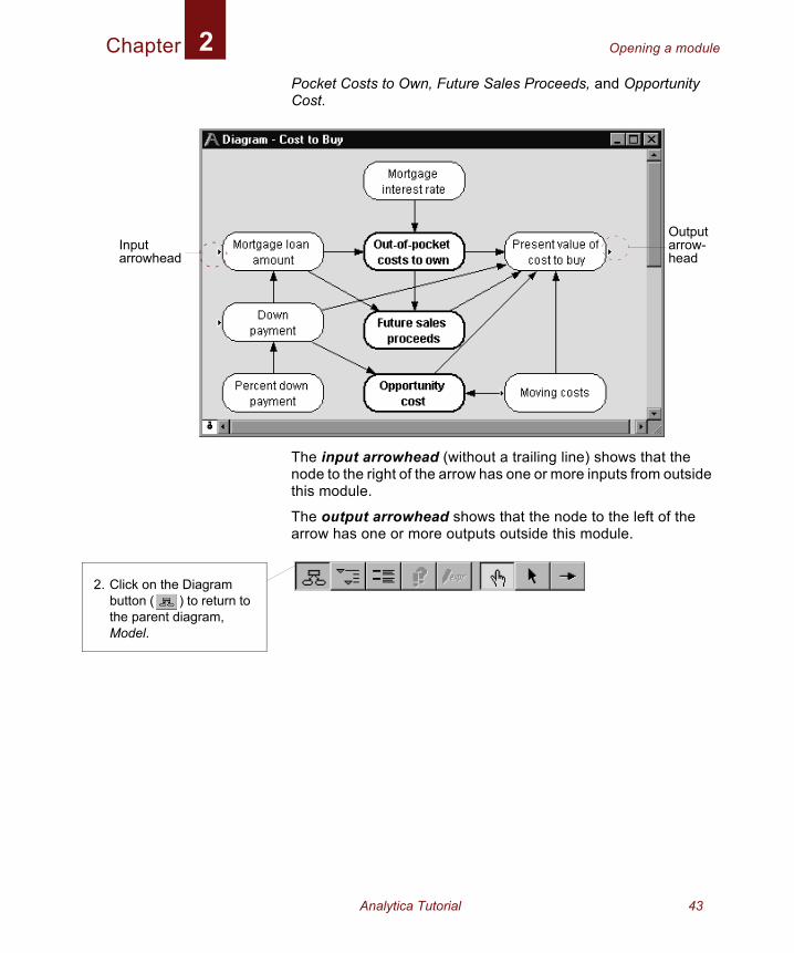
Pocket Costs to Own, Future Sales Proceeds, and Opportunity Cost.The input arrowhead (without a trailing line) shows that the node to the right of the arrow has one or more inputs from outside this module.
The output arrowhead shows that the node to the left of the arrow has one or more outputs outside this module.
Output arrow-head
Input arrowhead
2. Click on the Diagram button ( ) to return to the parent diagram, Model.
Analytica Tutorial 43
Chapter Opening a module2
4.
Analytica limits the number of open windows at each level of the model hierarchy to minimize clutter on your screen. See “Managing Windows” in Chapter 19 of the Analytica User Guide for information on how to open more than one module Diagram window at a time.
The combined arrowhead shows that the node has one or more inputs from outside this module, plus the input variable in this module.
3. Double-click on the Cost to Rent node to open the module.
The Cost to Rent diagram opens (see the figure below).
Combined arrowhead
Click on the Diagram button ( ) to return to the parent diagram, Model.
44 Analytica Tutorial
Chapter Opening a module2
5
6.
7
8
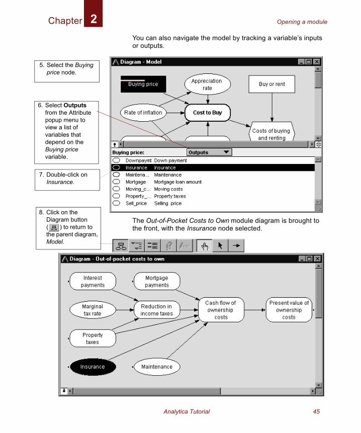
You can also navigate the model by tracking a variable’s inputs or outputs.
The Out-of-Pocket Costs to Own module diagram is brought to the front, with the Insurance node selected.
. Select the Buying price node.
Select Outputs from the Attribute popup menu to view a list of variables that depend on the Buying price variable.
. Double-click on Insurance.
. Click on the Diagram button ( ) to return to the parent diagram, Model.
Analytica Tutorial 45
Chapter Inspecting values in the Attribute panel2
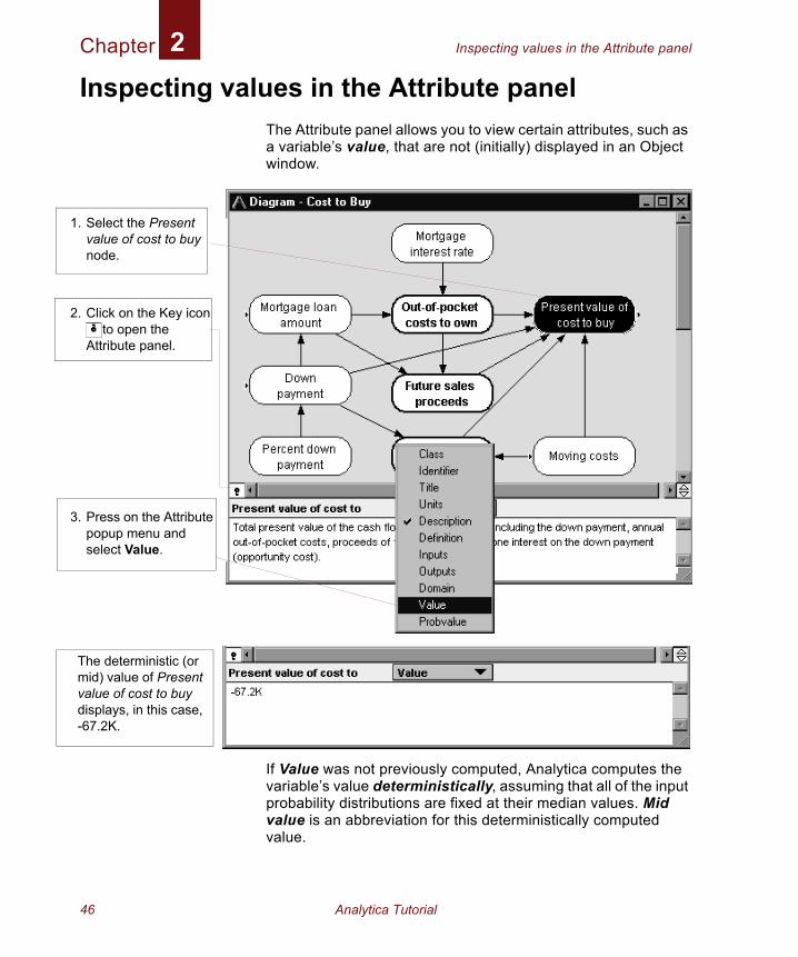
Inspecting values in the Attribute panelThe Attribute panel allows you to view certain attributes, such as a variable’s value, that are not (initially) displayed in an Object window.
If Value was not previously computed, Analytica computes the variable’s value deterministically, assuming that all of the input probability distributions are fixed at their median values. Mid value is an abbreviation for this deterministically computed value.
1. Select the Present value of cost to buy node.
2. Click on the Key icon( ) to open the Attribute panel.
3. Press on the Attribute popup menu and select Value.
The deterministic (or mid) value of Present value of cost to buy displays, in this case, -67.2K.
46 Analytica Tutorial
Chapter Displaying results2
1. WcoseRto
You can use the Attribute panel in this manner to examine the mid value of any variable in the model.
It is faster to compute a mid (deterministic) value than an uncertain (probabilistic) value, so it is useful for conducting initial checks of a model before performing any uncertainty analysis.
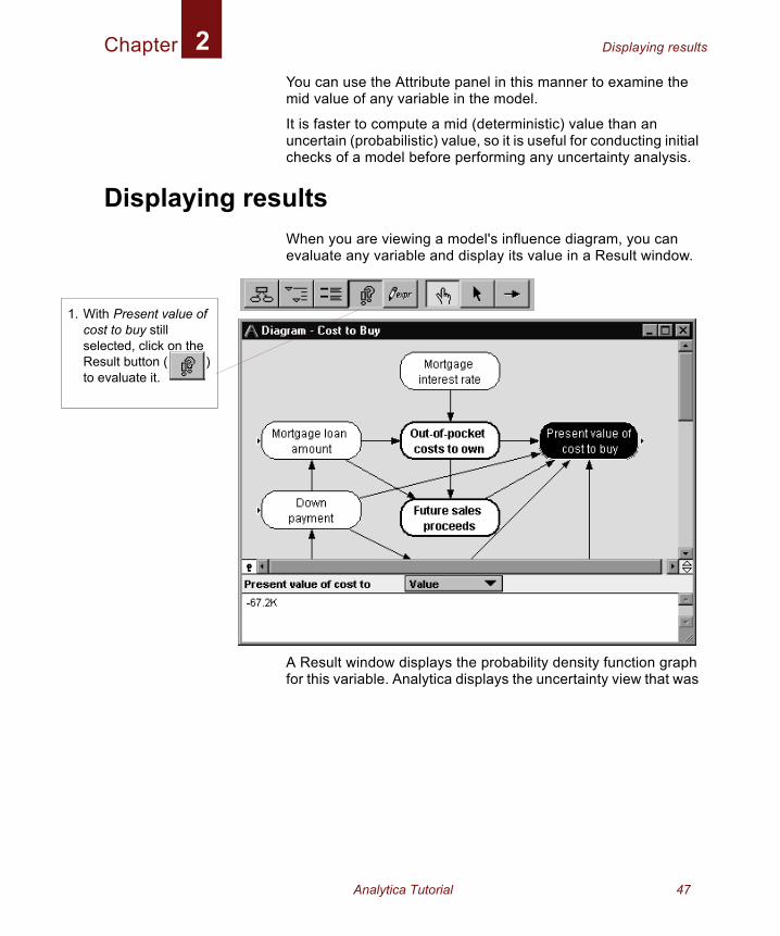
Displaying resultsWhen you are viewing a model's influence diagram, you can evaluate any variable and display its value in a Result window.
A Result window displays the probability density function graph for this variable. Analytica displays the uncertainty view that was
ith Present value of st to buy still lected, click on the
esult button ( ) evaluate it.
Analytica Tutorial 47
Chapter Displaying results2
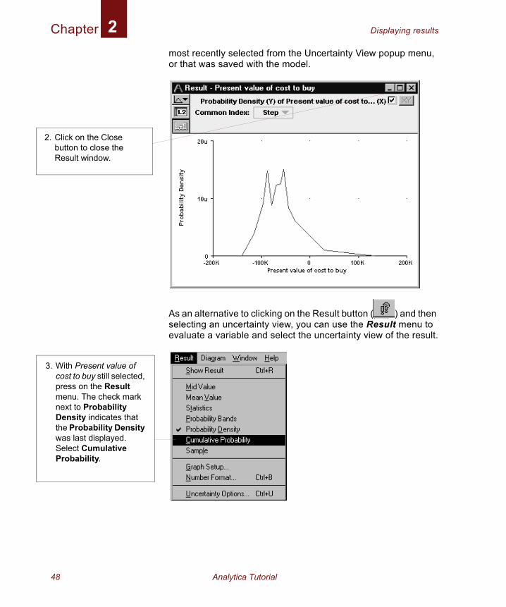
most recently selected from the Uncertainty View popup menu, or that was saved with the model.As an alternative to clicking on the Result button ( ) and then selecting an uncertainty view, you can use the Result menu to evaluate a variable and select the uncertainty view of the result.
2. Click on the Close button to close the Result window.
3. With Present value of cost to buy still selected, press on the Result menu. The check mark next to Probability Density indicates that the Probability Density was last displayed. Select Cumulative Probability.
48 Analytica Tutorial
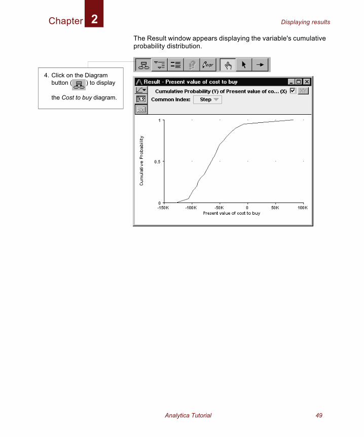
Chapter Displaying results2
The Result window appears displaying the variable's cumulative probability distribution.4. Click on the Diagram button ( ) to display
the Cost to buy diagram.
Analytica Tutorial 49
Chapter Displaying results2
5
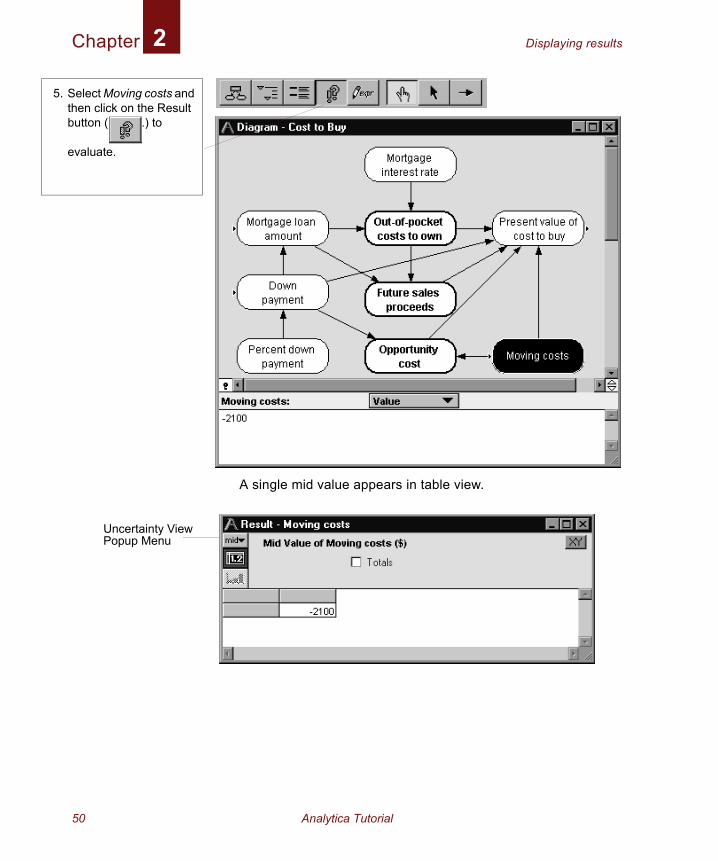
A single mid value appears in table view.
. Select Moving costs and then click on the Resultbutton (...........) to
evaluate.
Uncertainty View Popup Menu
50 Analytica Tutorial
Chapter Exploring the Rent vs. Buy model: Summary2
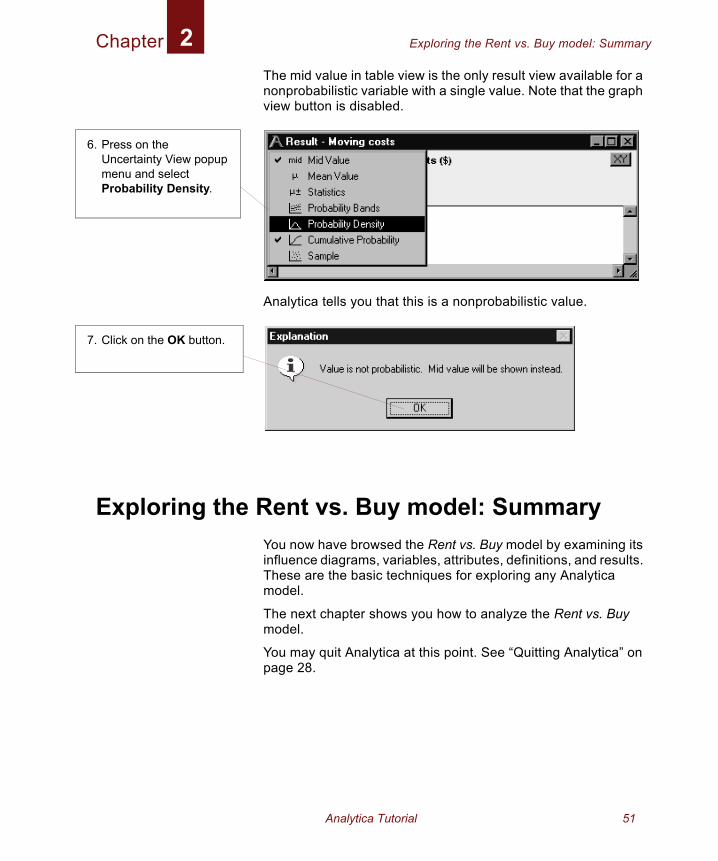
The mid value in table view is the only result view available for a nonprobabilistic variable with a single value. Note that the graph view button is disabled.Analytica tells you that this is a nonprobabilistic value.
Exploring the Rent vs. Buy model: SummaryYou now have browsed the Rent vs. Buy model by examining its influence diagrams, variables, attributes, definitions, and results. These are the basic techniques for exploring any Analytica model.
The next chapter shows you how to analyze the Rent vs. Buy model.
You may quit Analytica at this point. See “Quitting Analytica” on page 28.
6. Press on the Uncertainty View popup menu and select Probability Density.
7. Click on the OK button.
Analytica Tutorial 51

Chapter Exploring the Rent vs. Buy Model Exploring the Rent vs. Buy 8
52 Analytica Tutorial
Chapter 3
Analyzing the Rent vs. Buy Analysis Model

In this Chapter
This chapter shows you how to:
• Perform importance analysis
• Perform parametric analysis
• Set up and compare alternative decisions
Chapter 3:Analyzing the Rent vs. Buy Analysis ModelIn this chapter you will analyze the Rent vs. Buy Analysis model, a modified version of the model that you used in Chapter 1: Using the Rent vs. Buy Model and Chapter 2: Exploring the Rent vs.Buy Model. You will identify its key sources of uncertainty through importance analysis, perform parametric analysis, and compare alternative decisions.
For instructions on how to open a model, see “Opening the Rent vs. Buy model” on page 11. In this case, however, open the Rent vs. Buy Analysis model by double-clicking on the icon labeled Rent vs. Buy Analysis.ana.
Examining the difference between renting and buying
The Rent vs. Buy Analysis model is the module called Model that you explored in Chapter 2: Exploring the Rent vs.Buy Model, with the addition of nodes to help you understand the importance of the uncertain inputs to the uncertainty in the output.
In Chapter 1: Using the Rent vs. Buy Model, you saw that evaluating Costs of buying and renting produces a graph of two uncertain values. To understand whether it would be financially advantageous to rent or buy, the Rent vs. Buy Analysis model
Analytica Tutorial 55
Chapter Examining the difference between renting and buying3
1. Cbere
2. C(
ev
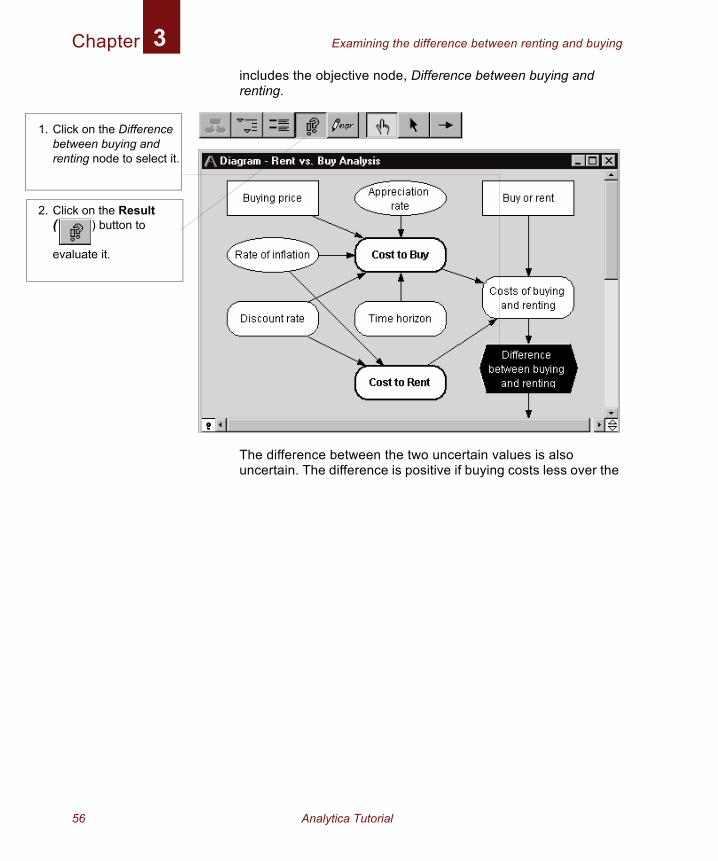
includes the objective node, Difference between buying and renting.
The difference between the two uncertain values is also uncertain. The difference is positive if buying costs less over the
lick on the Difference tween buying and nting node to select it.
lick on the Result ) button to
aluate it.
56 Analytica Tutorial
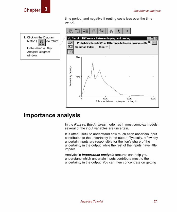
Chapter Importance analysis3
time period, and negative if renting costs less over the time period.Importance analysisIn the Rent vs. Buy Analysis model, as in most complex models, several of the input variables are uncertain.
It is often useful to understand how much each uncertain input contributes to the uncertainty in the output. Typically, a few key uncertain inputs are responsible for the lion’s share of the uncertainty in the output, while the rest of the inputs have little impact.
Analytica’s importance analysis features can help you understand which uncertain inputs contribute most to the uncertainty in the output. You can then concentrate on getting
1. Click on the Diagram button ( ) to return
to the Rent vs. Buy Analysis Diagram window.
Analytica Tutorial 57
Chapter Importance analysis3
1. Sebere
2. Clbudith
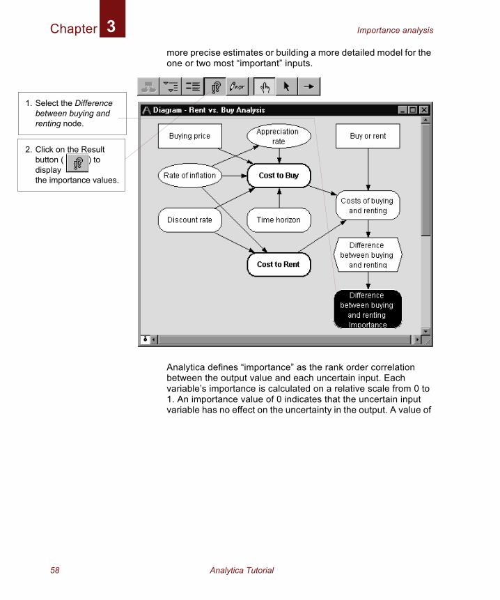
more precise estimates or building a more detailed model for the one or two most “important” inputs.
Analytica defines “importance” as the rank order correlation between the output value and each uncertain input. Each variable’s importance is calculated on a relative scale from 0 to 1. An importance value of 0 indicates that the uncertain input variable has no effect on the uncertainty in the output. A value of
lect the Difference tween buying and nting node.
ick on the Result tton ( ) to
splaye importance values.
58 Analytica Tutorial
Chapter Importance analysis3
3. CburetoAw
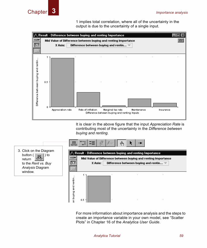
1 implies total correlation, where all of the uncertainty in the output is due to the uncertainty of a single input.
It is clear in the above figure that the input Appreciation Rate is contributing most of the uncertainty in the Difference between buying and renting.
For more information about importance analysis and the steps to create an importance variable in your own model, see “Scatter Plots” in Chapter 16 of the Analytica User Guide.
lick on the Diagram tton ( ) to turn the Rent vs. Buy nalysis Diagram indow.
Analytica Tutorial 59
Chapter Performing parametric (sensitivity) analysis3
1
2
Performing parametric (sensitivity) analysisParametric analysis (also called sensitivity analysis) involves varying the value of an input variable to examine its effect on a selected output. Performing sensitivity analysis often provides useful insights into how small changes in input variable values affect the desired outcome.
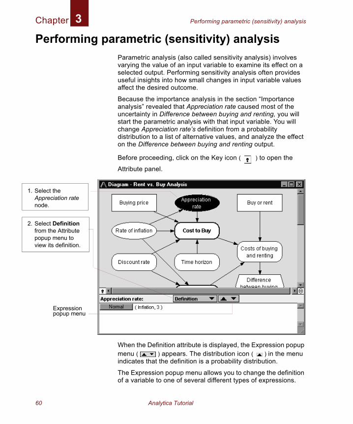
Because the importance analysis in the section “Importance analysis” revealed that Appreciation rate caused most of the uncertainty in Difference between buying and renting, you will start the parametric analysis with that input variable. You will change Appreciation rate’s definition from a probability distribution to a list of alternative values, and analyze the effect on the Difference between buying and renting output.
Before proceeding, click on the Key icon ( ) to open the
Attribute panel.
When the Definition attribute is displayed, the Expression popup menu ( ) appears. The distribution icon ( ) in the menu indicates that the definition is a probability distribution.
The Expression popup menu allows you to change the definition of a variable to one of several different types of expressions.
. Select the Appreciation rate node.
. Select Definition from the Attribute popup menu to view its definition.
Expression popup menu
60 Analytica Tutorial
Chapter Performing parametric (sensitivity) analysis3
3.
4.
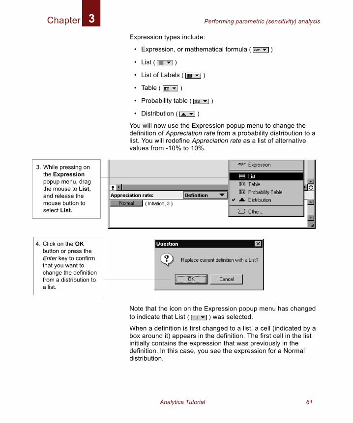
Expression types include:
• Expression, or mathematical formula ( )
• List ( )
• List of Labels ( )
• Table ( )
• Probability table ( )
• Distribution ( )
You will now use the Expression popup menu to change the definition of Appreciation rate from a probability distribution to a list. You will redefine Appreciation rate as a list of alternative values from -10% to 10%.
Note that the icon on the Expression popup menu has changed to indicate that List ( ) was selected.
When a definition is first changed to a list, a cell (indicated by a box around it) appears in the definition. The first cell in the list initially contains the expression that was previously in the definition. In this case, you see the expression for a Normal distribution.
While pressing on the Expression popup menu, drag the mouse to List, and release the mouse button to select List.
Click on the OK button or press the Enter key to confirm that you want to change the definition from a distribution to a list.
Analytica Tutorial 61
Chapter Performing parametric (sensitivity) analysis3
5. Scvt
6.
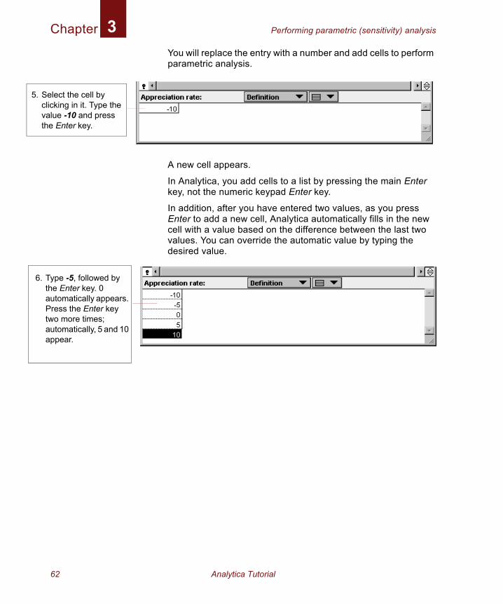
You will replace the entry with a number and add cells to perform parametric analysis.
A new cell appears.
In Analytica, you add cells to a list by pressing the main Enter key, not the numeric keypad Enter key.
In addition, after you have entered two values, as you press Enter to add a new cell, Analytica automatically fills in the new cell with a value based on the difference between the last two values. You can override the automatic value by typing the desired value.
elect the cell by licking in it. Type the alue -10 and press he Enter key.
Type -5, followed by the Enter key. 0 automatically appears. Press the Enter key two more times; automatically, 5 and 10 appear.
62 Analytica Tutorial
Chapter Performing parametric (sensitivity) analysis3
7.
8.
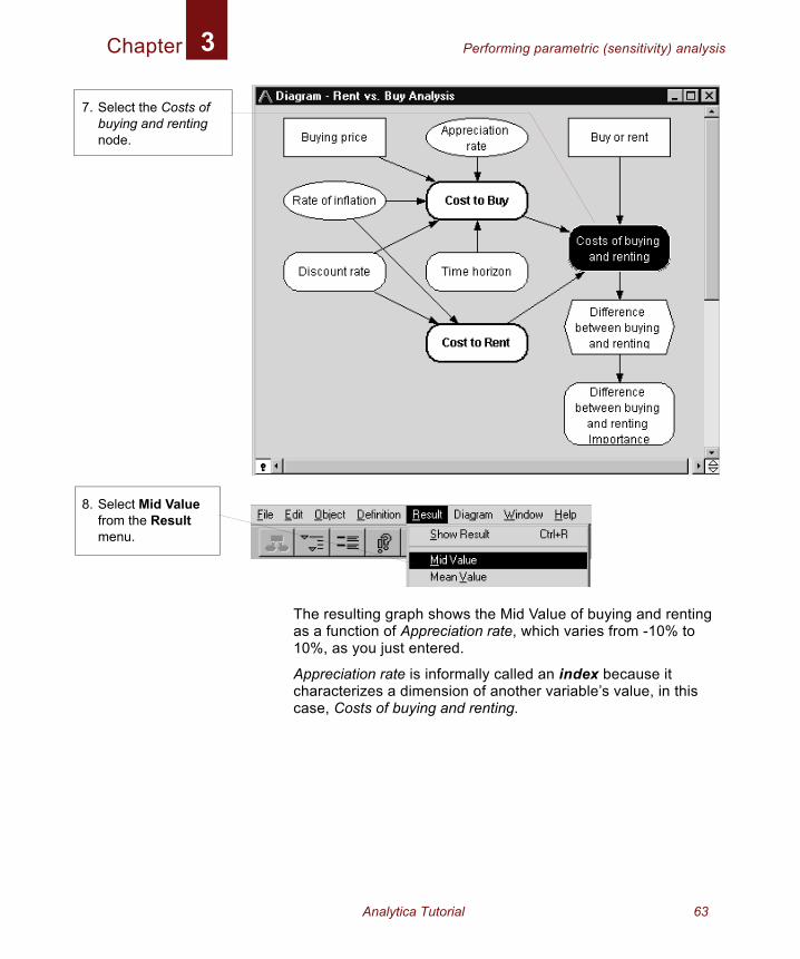
The resulting graph shows the Mid Value of buying and renting as a function of Appreciation rate, which varies from -10% to 10%, as you just entered.
Appreciation rate is informally called an index because it characterizes a dimension of another variable’s value, in this case, Costs of buying and renting.
Select the Costs of buying and renting node.
Select Mid Value from the Result menu.
Analytica Tutorial 63
Chapter Performing parametric (sensitivity) analysis3
1
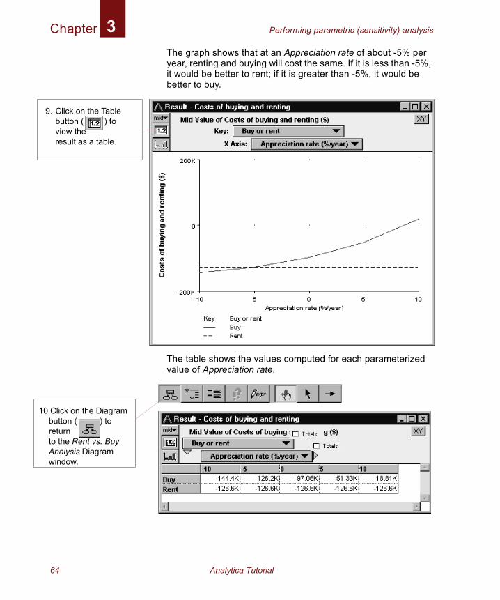
The graph shows that at an Appreciation rate of about -5% per year, renting and buying will cost the same. If it is less than -5%, it would be better to rent; if it is greater than -5%, it would be better to buy.
The table shows the values computed for each parameterized value of Appreciation rate.
9. Click on the Table button ( ) toview theresult as a table.
0.Click on the Diagram button ( ) to returnto the Rent vs. Buy Analysis Diagram window.
64 Analytica Tutorial
Chapter Performing parametric (sensitivity) analysis3
1.
2.
3. Ct
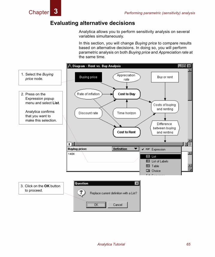
Evaluating alternative decisionsAnalytica allows you to perform sensitivity analysis on several variables simultaneously.
In this section, you will change Buying price to compare results based on alternative decisions. In doing so, you will perform parametric analysis on both Buying price and Appreciation rate at the same time.
Select the Buying price node.
Press on the Expression popup menu and select List.
Analytica confirms that you want to make this selection.
lick on the OK button o proceed.
Analytica Tutorial 65
Chapter Performing parametric (sensitivity) analysis3
4. Csak
5. Tb
1ec
6.
7. Sthreit
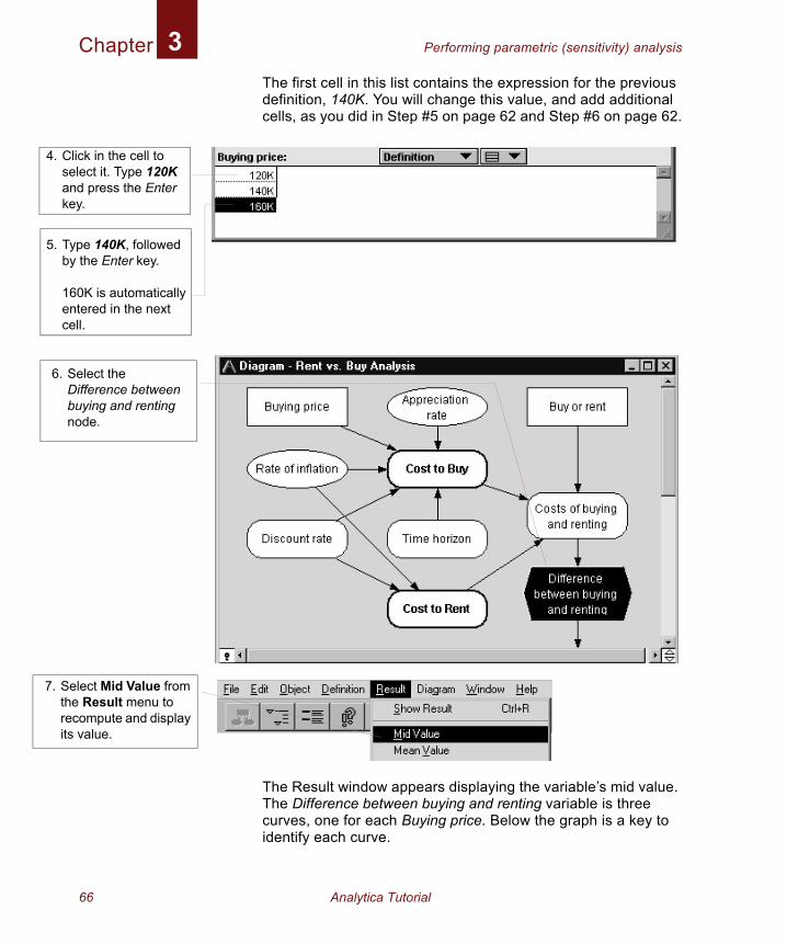
The first cell in this list contains the expression for the previous definition, 140K. You will change this value, and add additional cells, as you did in Step #5 on page 62 and Step #6 on page 62.
The Result window appears displaying the variable’s mid value. The Difference between buying and renting variable is three curves, one for each Buying price. Below the graph is a key to identify each curve.
lick in the cell to elect it. Type 120K nd press the Enter ey.
ype 140K, followed y the Enter key.
60K is automatically ntered in the next ell.
Select the Difference between buying and renting node.
elect Mid Value from e Result menu to compute and display
s value.
66 Analytica Tutorial
Chapter Performing parametric (sensitivity) analysis3
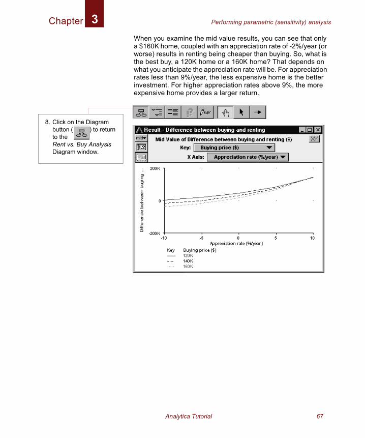
When you examine the mid value results, you can see that only a $160K home, coupled with an appreciation rate of -2%/year (or worse) results in renting being cheaper than buying. So, what is the best buy, a 120K home or a 160K home? That depends on what you anticipate the appreciation rate will be. For appreciation rates less than 9%/year, the less expensive home is the better investment. For higher appreciation rates above 9%, the more expensive home provides a larger return.8. Click on the Diagram button ( ) to return to theRent vs. Buy Analysis Diagram window.
Analytica Tutorial 67
Chapter Performing parametric (sensitivity) analysis3
9. Sbn
10
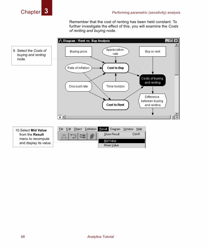
Remember that the cost of renting has been held constant. To further investigate the effect of this, you will examine the Costs of renting and buying node.
elect the Costs of uying and renting ode.
.Select Mid Value from the Result menu to recompute and display its value.
68 Analytica Tutorial
Chapter Performing parametric (sensitivity) analysis3
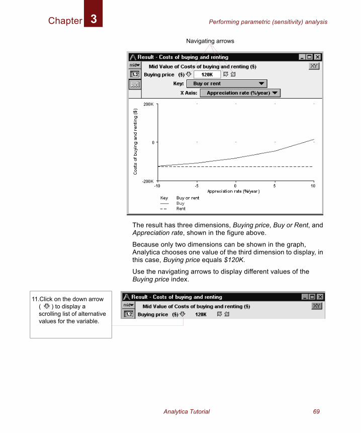
11.C(scva
The result has three dimensions, Buying price, Buy or Rent, and Appreciation rate, shown in the figure above.
Because only two dimensions can be shown in the graph, Analytica chooses one value of the third dimension to display, in this case, Buying price equals $120K.
Use the navigating arrows to display different values of the Buying price index.
Navigating arrows
lick on the down arrow ) to display a
rolling list of alternative lues for the variable.
Analytica Tutorial 69
Chapter Performing parametric (sensitivity) analysis3
12.s
13
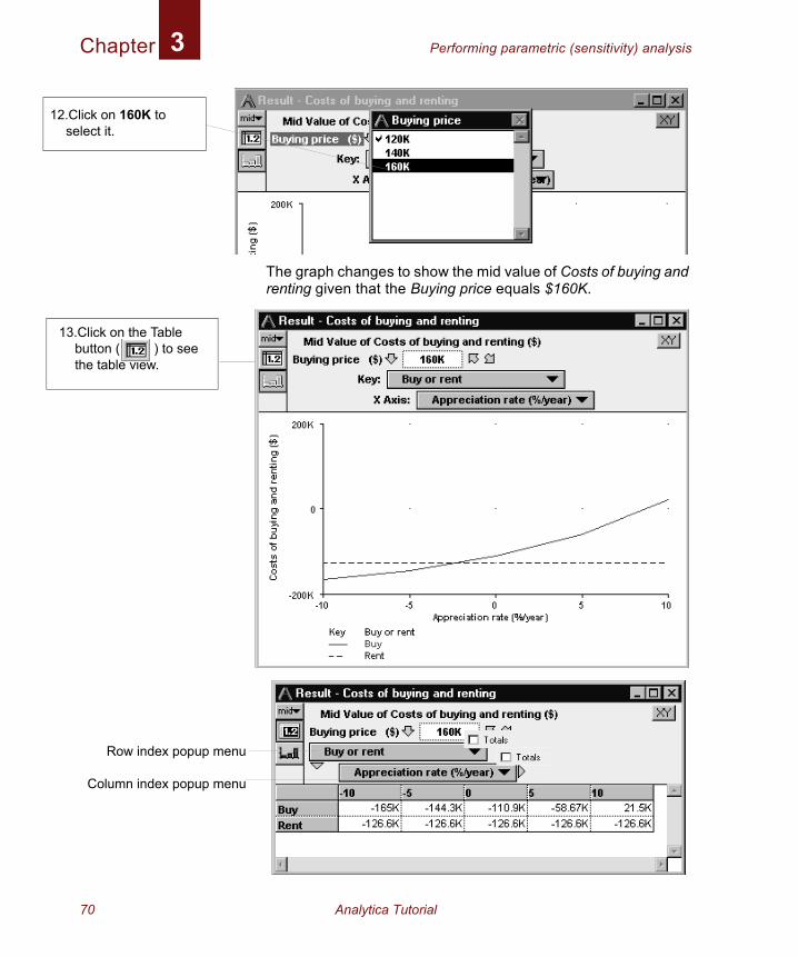
The graph changes to show the mid value of Costs of buying and renting given that the Buying price equals $160K.
Click on 160K to elect it.
.Click on the Table button ( ) to see the table view.
Row index popup menu
Column index popup menu
70 Analytica Tutorial
Chapter Performing parametric (sensitivity) analysis3
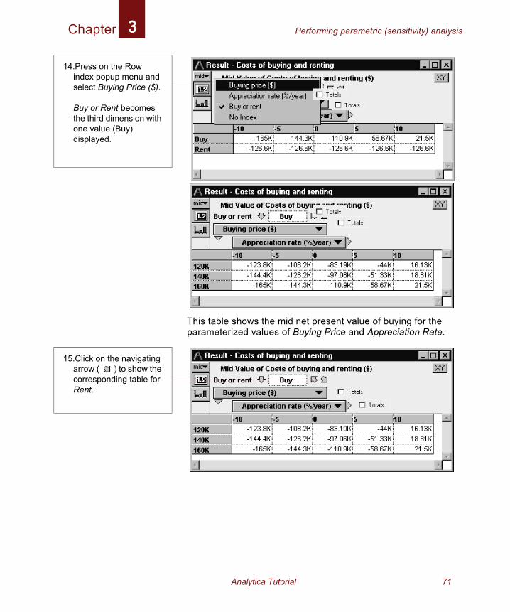
This table shows the mid net present value of buying for the parameterized values of Buying Price and Appreciation Rate.
14.Press on the Row index popup menu and select Buying Price ($).
Buy or Rent becomes the third dimension with one value (Buy) displayed.
15.Click on the navigating arrow ( ) to show the corresponding table for Rent.
Analytica Tutorial 71
Chapter Analyzing the Rent vs. Buy Analysis model: Summary3
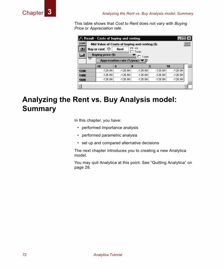
This table shows that Cost to Rent does not vary with Buying Price or Appreciation rate.Analyzing the Rent vs. Buy Analysis model: Summary
In this chapter, you have:
• performed importance analysis
• performed parametric analysis
• set up and compared alternative decisions
The next chapter introduces you to creating a new Analytica model.
You may quit Analytica at this point. See “Quitting Analytica” on page 28.
72 Analytica Tutorial

Chapter 4
Creating a Model

In this Chapter
This chapter shows you how to:
• Create a model
• Document and define variables
• Create a module
• Draw arrows between variables
1
2
3
Chapter 4: Creating a ModelThis chapter introduces you to creating a new Analytica model.
In the process of building a model that analyzes the costs of owning and operating an automobile, you will create variables, define dependencies, add documentary text, and compute results. In addition, you will create modules.
Start Analytica by double-clicking on its icon as described in “Opening the Rent vs. Buy model” beginning on page 11. Analytica opens with a blank new model.
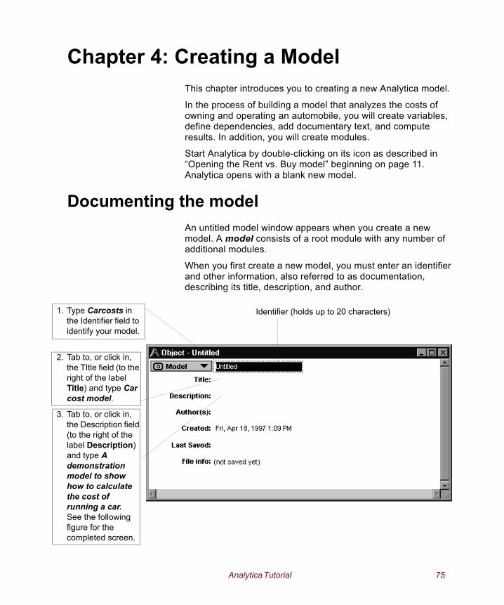
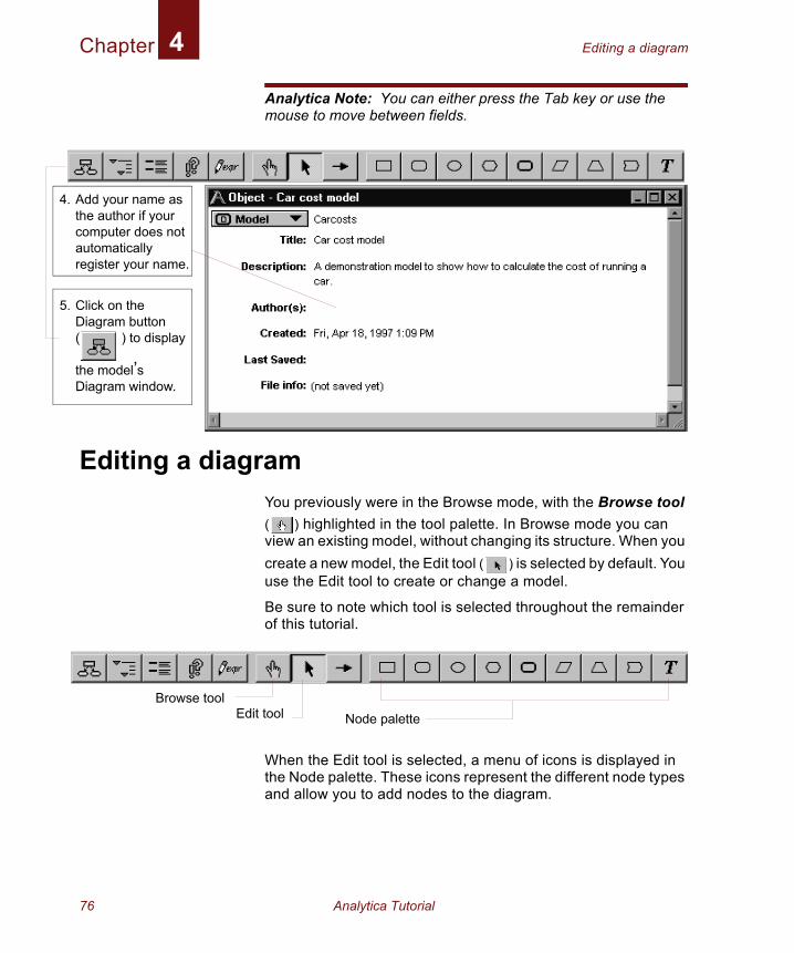
Documenting the modelAn untitled model window appears when you create a new model. A model consists of a root module with any number of additional modules.
When you first create a new model, you must enter an identifier and other information, also referred to as documentation, describing its title, description, and author.
. Type Carcosts in the Identifier field to identify your model.
. Tab to, or click in, the TItle field (to the right of the label Title) and type Car cost model.
. Tab to, or click in, the Description field (to the right of the label Description) and type A demonstration model to show how to calculate the cost of running a car.See the following figure for the completed screen.
Identifier (holds up to 20 characters)
Analytica Tutorial 75
Chapter Editing a diagram4
4
5
Analytica Note: You can either press the Tab key or use the mouse to move between fields.
Editing a diagramYou previously were in the Browse mode, with the Browse tool ( ) highlighted in the tool palette. In Browse mode you can view an existing model, without changing its structure. When you create a new model, the Edit tool ( ) is selected by default. You use the Edit tool to create or change a model.
Be sure to note which tool is selected throughout the remainder of this tutorial.
When the Edit tool is selected, a menu of icons is displayed in the Node palette. These icons represent the different node types and allow you to add nodes to the diagram.
. Add your name as the author if your computer does not automatically register your name.
. Click on the Diagram button ( ) to display
the model’s Diagram window.
Browse toolEdit tool Node palette
76 Analytica Tutorial
Chapter Creating variables4
1. D(
th
Aaaybpc
2. Tyva
Ponthth
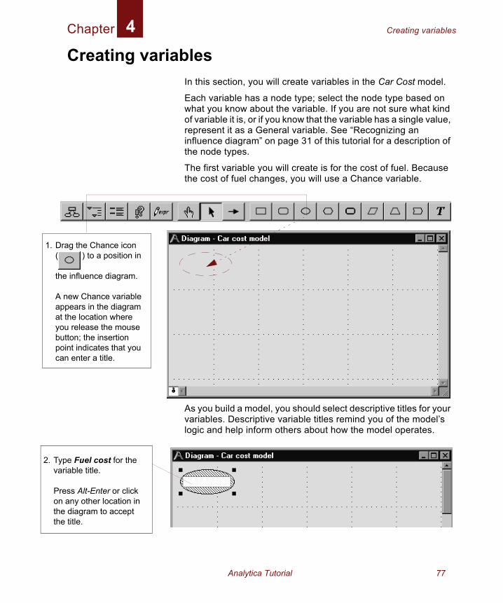
Creating variablesIn this section, you will create variables in the Car Cost model.
Each variable has a node type; select the node type based on what you know about the variable. If you are not sure what kind of variable it is, or if you know that the variable has a single value, represent it as a General variable. See “Recognizing an influence diagram” on page 31 of this tutorial for a description of the node types.
The first variable you will create is for the cost of fuel. Because the cost of fuel changes, you will use a Chance variable.
As you build a model, you should select descriptive titles for your variables. Descriptive variable titles remind you of the model’s logic and help inform others about how the model operates.
rag the Chance icon ) to a position in
e influence diagram.
new Chance variable ppears in the diagram t the location where ou release the mouse utton; the insertion oint indicates that you an enter a title.
pe Fuel cost for the riable title.
ress Alt-Enter or click any other location in
e diagram to accept e title.
Analytica Tutorial 77
Chapter Creating variables4
3.
4.
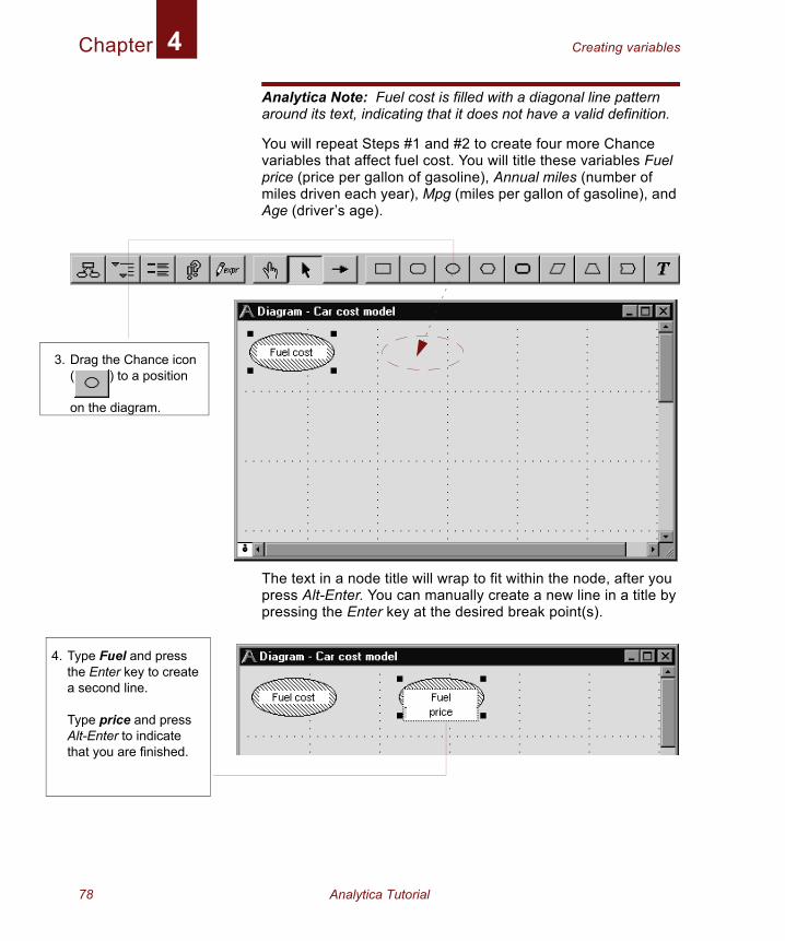
Analytica Note: Fuel cost is filled with a diagonal line pattern around its text, indicating that it does not have a valid definition.
You will repeat Steps #1 and #2 to create four more Chance variables that affect fuel cost. You will title these variables Fuel price (price per gallon of gasoline), Annual miles (number of miles driven each year), Mpg (miles per gallon of gasoline), and Age (driver’s age).
The text in a node title will wrap to fit within the node, after you press Alt-Enter. You can manually create a new line in a title by pressing the Enter key at the desired break point(s).
Drag the Chance icon ( ) to a position
on the diagram.
Type Fuel and press the Enter key to create a second line.
Type price and press Alt-Enter to indicate that you are finished.
78 Analytica Tutorial
Chapter Saving your model4
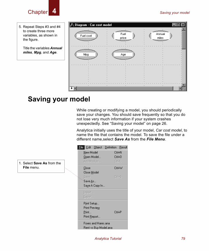
5. Rtovth
Tm
1. SF
Saving your modelWhile creating or modifying a model, you should periodically save your changes. You should save frequently so that you do not lose very much information if your system crashes unexpectedly. See “Saving your model” on page 26.
Analytica initially uses the title of your model, Car cost model, to name the file that contains the model. To save the file under a different name,select Save As from the File Menu.
epeat Steps #3 and #4 create three more
ariables, as shown in e figure.
itle the variables Annual iles, Mpg, and Age.
elect Save As from the ile menu.
Analytica Tutorial 79
Chapter Deleting a variable4
1
2
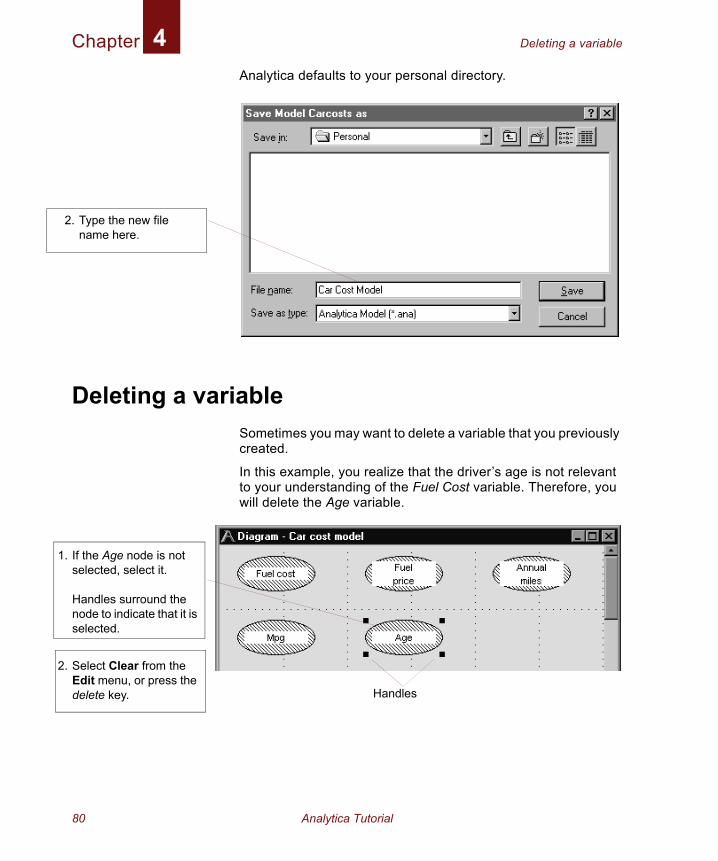
Analytica defaults to your personal directory.
Deleting a variableSometimes you may want to delete a variable that you previously created.
In this example, you realize that the driver’s age is not relevant to your understanding of the Fuel Cost variable. Therefore, you will delete the Age variable.
2. Type the new file name here.
. If the Age node is not selected, select it.
Handles surround the node to indicate that it is selected.
. Select Clear from the Edit menu, or press the delete key. Handles
80 Analytica Tutorial
Chapter Moving nodes4
3.
1.
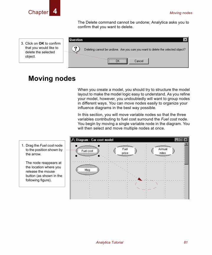
The Delete command cannot be undone; Analytica asks you to confirm that you want to delete.
Moving nodesWhen you create a model, you should try to structure the model layout to make the model logic easy to understand. As you refine your model, however, you undoubtedly will want to group nodes in different ways. You can move nodes easily to organize your influence diagrams in the best way possible.
In this section, you will move variable nodes so that the three variables contributing to fuel cost surround the Fuel cost node. You begin by moving a single variable node in the diagram. You will then select and move multiple nodes at once.
Click on OK to confirm that you would like to delete the selected object.
Drag the Fuel cost node to the position shown by the arrow.
The node reappears at the location where you release the mouse button (as shown in the following figure).
Analytica Tutorial 81
Chapter Moving nodes4
2.
3.
4.
5.
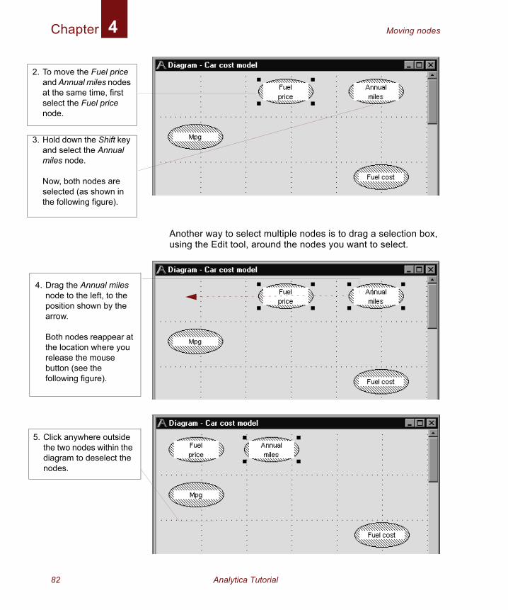
Another way to select multiple nodes is to drag a selection box, using the Edit tool, around the nodes you want to select.
To move the Fuel price and Annual miles nodes at the same time, first select the Fuel price node.
Hold down the Shift key and select the Annual miles node.
Now, both nodes are selected (as shown in the following figure).
Drag the Annual miles node to the left, to the position shown by the arrow.
Both nodes reappear at the location where you release the mouse button (see the following figure).
Click anywhere outside the two nodes within the diagram to deselect the nodes.
82 Analytica Tutorial
Chapter Editing variable titles4
Analytica Note: You can undo or redo a drag operation by selecting Undo/Redo from the Edit menu, or by typing the keyboard shortcut, Ctrl-Z.
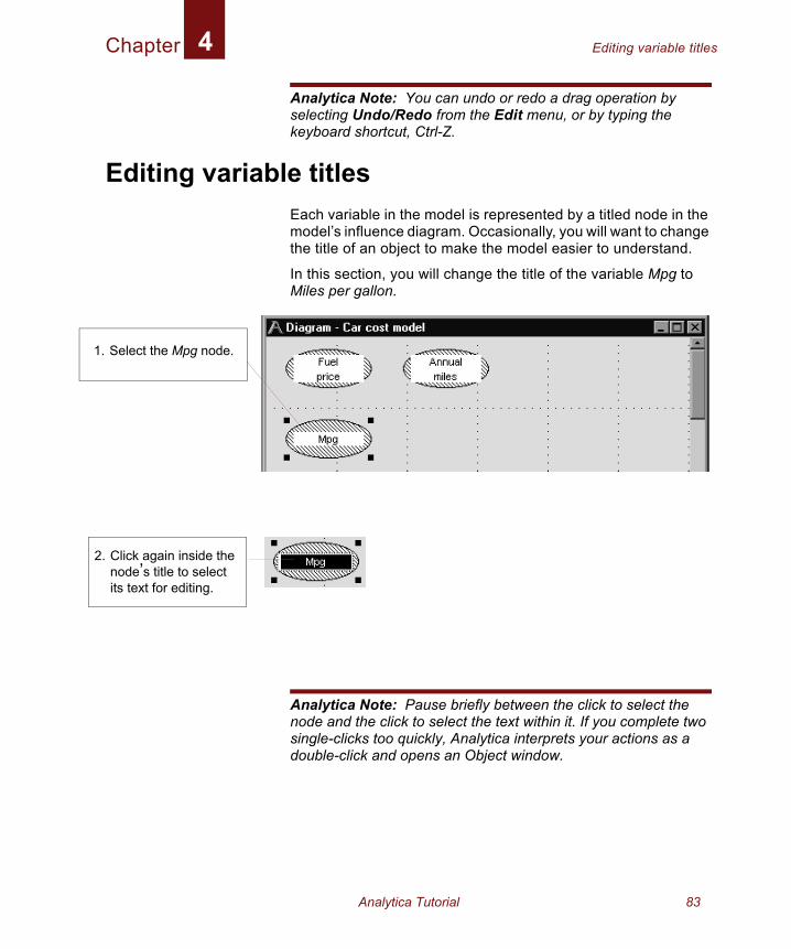
Editing variable titlesEach variable in the model is represented by a titled node in the model’s influence diagram. Occasionally, you will want to change the title of an object to make the model easier to understand.
In this section, you will change the title of the variable Mpg to Miles per gallon.
Analytica Note: Pause briefly between the click to select the node and the click to select the text within it. If you complete two single-clicks too quickly, Analytica interprets your actions as a double-click and opens an Object window.
1. Select the Mpg node.
2. Click again inside the node’s title to select its text for editing.
Analytica Tutorial 83
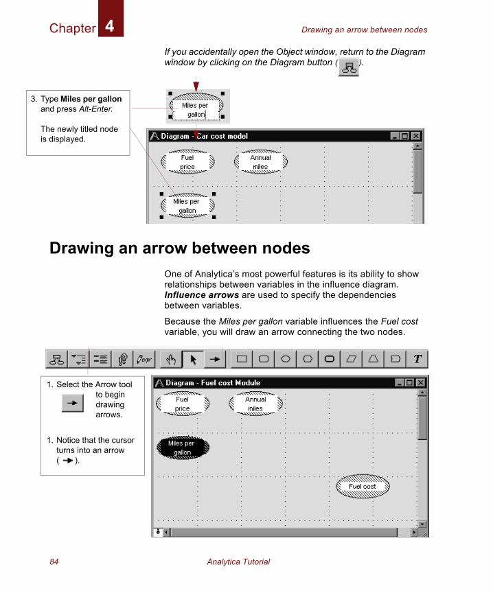
Chapter Drawing an arrow between nodes4
3. Ta
Ti
If you accidentally open the Object window, return to the Diagram window by clicking on the Diagram button ( ).
Drawing an arrow between nodesOne of Analytica’s most powerful features is its ability to show relationships between variables in the influence diagram. Influence arrows are used to specify the dependencies between variables.
Because the Miles per gallon variable influences the Fuel cost variable, you will draw an arrow connecting the two nodes.
ype Miles per gallon nd press Alt-Enter.
he newly titled node s displayed.
1. Select the Arrow tool to begin drawing arrows.
1. Notice that the cursor turns into an arrow ( ).
84 Analytica Tutorial
Chapter Deleting an arrow4
If the nodes are not connected by an arrow, repeat Steps #1 through #3.
Deleting an arrowOccasionally, you may need to delete an arrow because of an earlier mistake or a change in your understanding of the model. This section shows you how to delete the arrow that connects Miles per gallon to Fuel cost.
You can delete an arrow using either the Edit tool or the arrow tool.
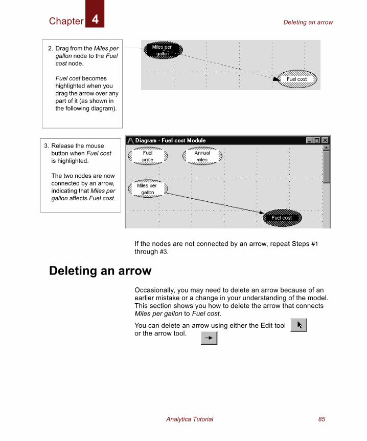
2. Drag from the Miles per gallon node to the Fuel cost node.
Fuel cost becomes highlighted when you drag the arrow over any part of it (as shown in the following diagram).
3. Release the mouse button when Fuel cost is highlighted.
The two nodes are now connected by an arrow, indicating that Miles per gallon affects Fuel cost.
Analytica Tutorial 85
Chapter Connecting multiple arrows4
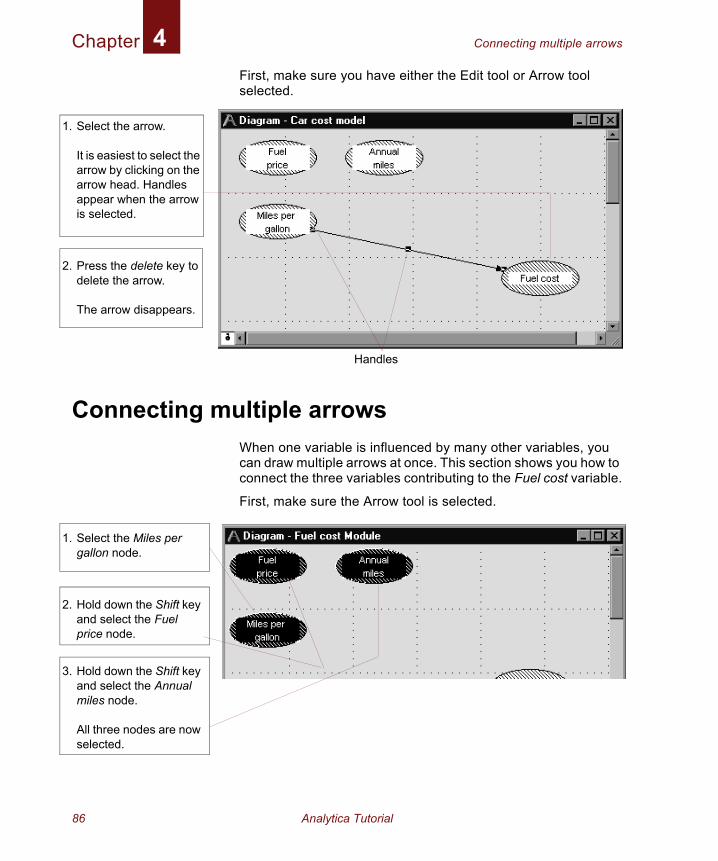
First, make sure you have either the Edit tool or Arrow tool selected.Connecting multiple arrowsWhen one variable is influenced by many other variables, you can draw multiple arrows at once. This section shows you how to connect the three variables contributing to the Fuel cost variable.
First, make sure the Arrow tool is selected.
1. Select the arrow.
It is easiest to select the arrow by clicking on the arrow head. Handles appear when the arrow is selected.
2. Press the delete key to delete the arrow.
The arrow disappears.
Handles
1. Select the Miles per gallon node.
2. Hold down the Shift key and select the Fuel price node.
3. Hold down the Shift key and select the Annual miles node.
All three nodes are now selected.
86 Analytica Tutorial
Chapter Connecting multiple arrows4
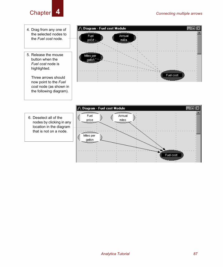
4. Drag from any one of the selected nodes to the Fuel cost node.
5. Release the mouse button when the Fuel cost node is highlighted.
Three arrows should now point to the Fuel cost node (as shown in the following diagram).
6. Deselect all of the nodes by clicking in any location in the diagram that is not on a node.
Analytica Tutorial 87
Chapter Entering attributes using the Object window4
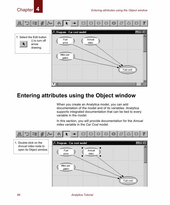
Entering attributes using the Object windowWhen you create an Analytica model, you can add documentation of the model and of its variables. Analytica supports integrated documentation that can be tied to every variable in the model.
In this section, you will provide documentation for the Annual miles variable in the Car Cost model.
7. Select the Edit button () to turn off arrow drawing.
1. Double-click on the Annual miles node to open its Object window.
88 Analytica Tutorial
Chapter Entering attributes using the Object window4
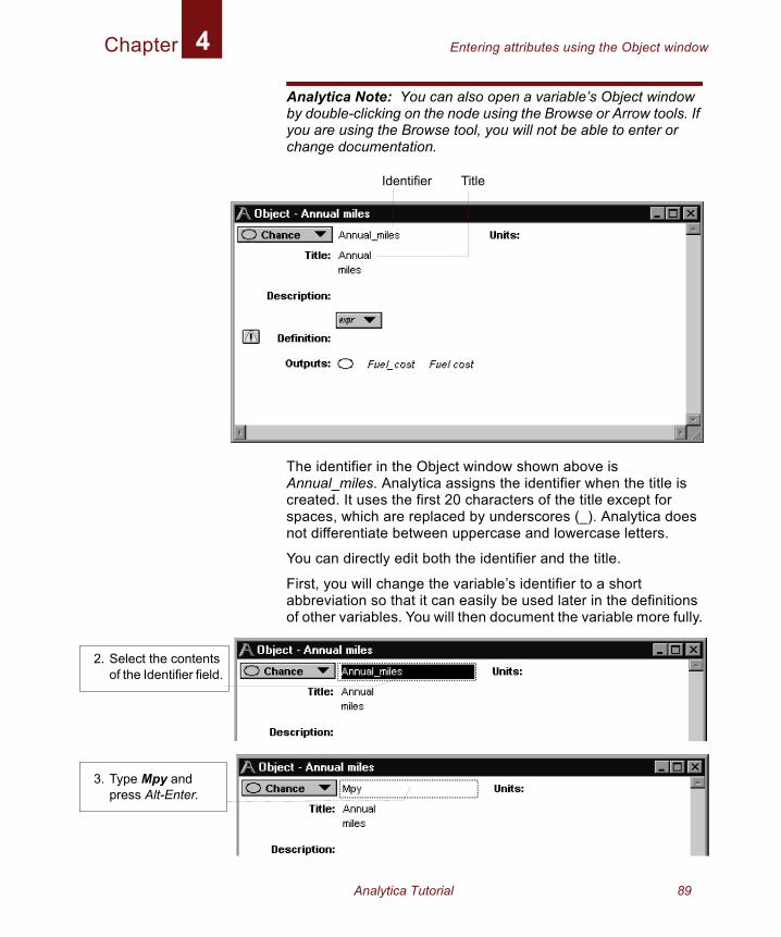
Analytica Note: You can also open a variable’s Object window by double-clicking on the node using the Browse or Arrow tools. If you are using the Browse tool, you will not be able to enter or change documentation.
The identifier in the Object window shown above is Annual_miles. Analytica assigns the identifier when the title is created. It uses the first 20 characters of the title except for spaces, which are replaced by underscores (_). Analytica does not differentiate between uppercase and lowercase letters.
You can directly edit both the identifier and the title.
First, you will change the variable’s identifier to a short abbreviation so that it can easily be used later in the definitions of other variables. You will then document the variable more fully.
Identifier Title
2. Select the contents of the Identifier field.
3. Type Mpy and press Alt-Enter.
Analytica Tutorial 89
Chapter Defining a variable explicitly4
7
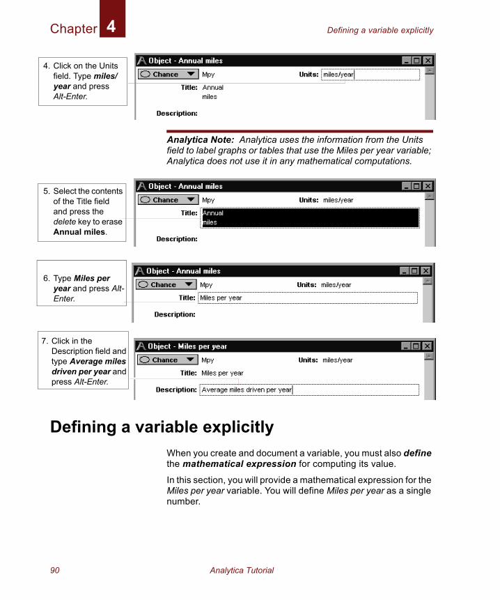
Analytica Note: Analytica uses the information from the Units field to label graphs or tables that use the Miles per year variable; Analytica does not use it in any mathematical computations.
Defining a variable explicitlyWhen you create and document a variable, you must also define the mathematical expression for computing its value.
In this section, you will provide a mathematical expression for the Miles per year variable. You will define Miles per year as a single number.
4. Click on the Units field. Type miles/year and press Alt-Enter.
5. Select the contents of the Title field and press the delete key to erase Annual miles.
6. Type Miles per year and press Alt-Enter.
. Click in the Description field and type Average miles driven per year and press Alt-Enter.
90 Analytica Tutorial
Chapter Defining a variable explicitly4
1
2
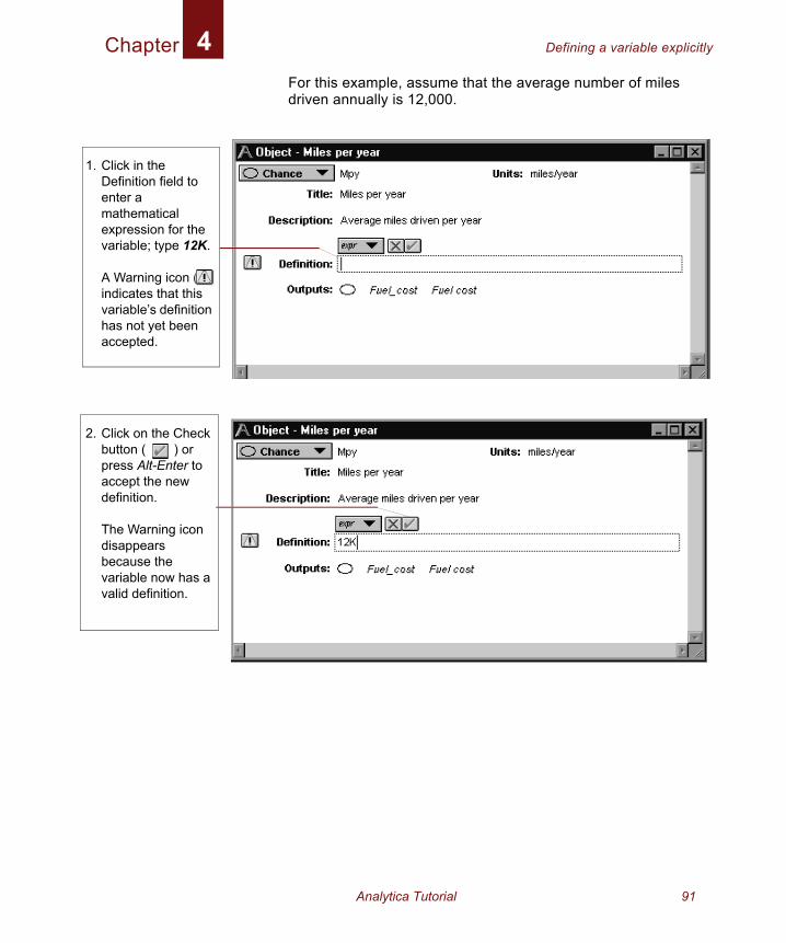
For this example, assume that the average number of miles driven annually is 12,000.
. Click in the Definition field to enter a mathematical expression for the variable; type 12K.
A Warning icon () indicates that this variable’s definition has not yet been accepted.
. Click on the Check button ( ) or press Alt-Enter to accept the new definition.
The Warning icon disappears because the variable now has a valid definition.
Analytica Tutorial 91
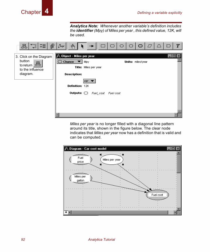
Chapter Defining a variable explicitly4
3
Analytica Note: Whenever another variable’s definition includes the identifier (Mpy) of Miles per year , this defined value, 12K, will be used.
Miles per year is no longer filled with a diagonal line pattern around its title, shown in the figure below. The clear node indicates that Miles per year now has a definition that is valid and can be computed.
. Click on the Diagram button to return to the influence diagram.
92 Analytica Tutorial
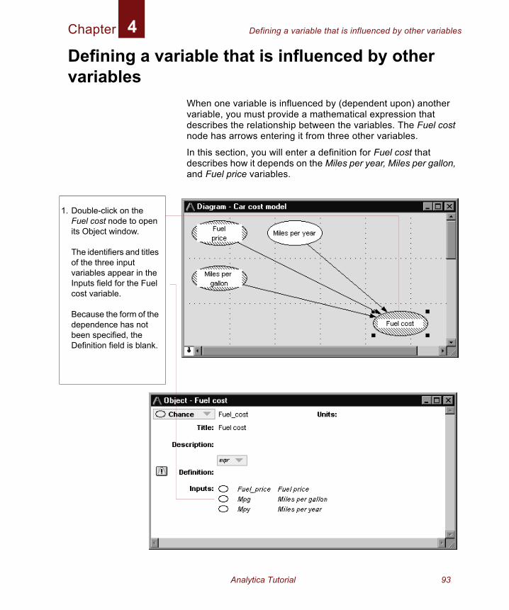
Chapter Defining a variable that is influenced by other variables4
Defining a variable that is influenced by other variablesWhen one variable is influenced by (dependent upon) another variable, you must provide a mathematical expression that describes the relationship between the variables. The Fuel cost node has arrows entering it from three other variables.
In this section, you will enter a definition for Fuel cost that describes how it depends on the Miles per year, Miles per gallon, and Fuel price variables.
1. Double-click on the Fuel cost node to open its Object window.
The identifiers and titles of the three input variables appear in the Inputs field for the Fuel cost variable.
Because the form of the dependence has not been specified, the Definition field is blank.
Analytica Tutorial 93
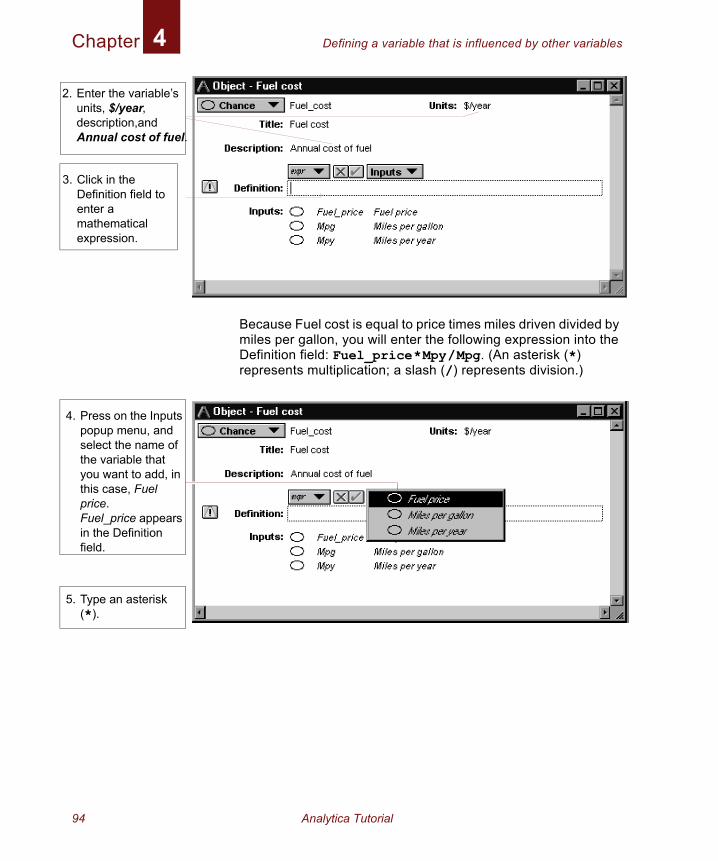
Chapter Defining a variable that is influenced by other variables4
Because Fuel cost is equal to price times miles driven divided by miles per gallon, you will enter the following expression into the Definition field: Fuel_price*Mpy/Mpg. (An asterisk (*) represents multiplication; a slash (/) represents division.)
2. Enter the variable’s units, $/year, description,and Annual cost of fuel.
3. Click in the Definition field to enter a mathematical expression.
4. Press on the Inputs popup menu, and select the name of the variable that you want to add, in this case, Fuel price.Fuel_price appears in the Definition field.
5. Type an asterisk (*).
94 Analytica Tutorial
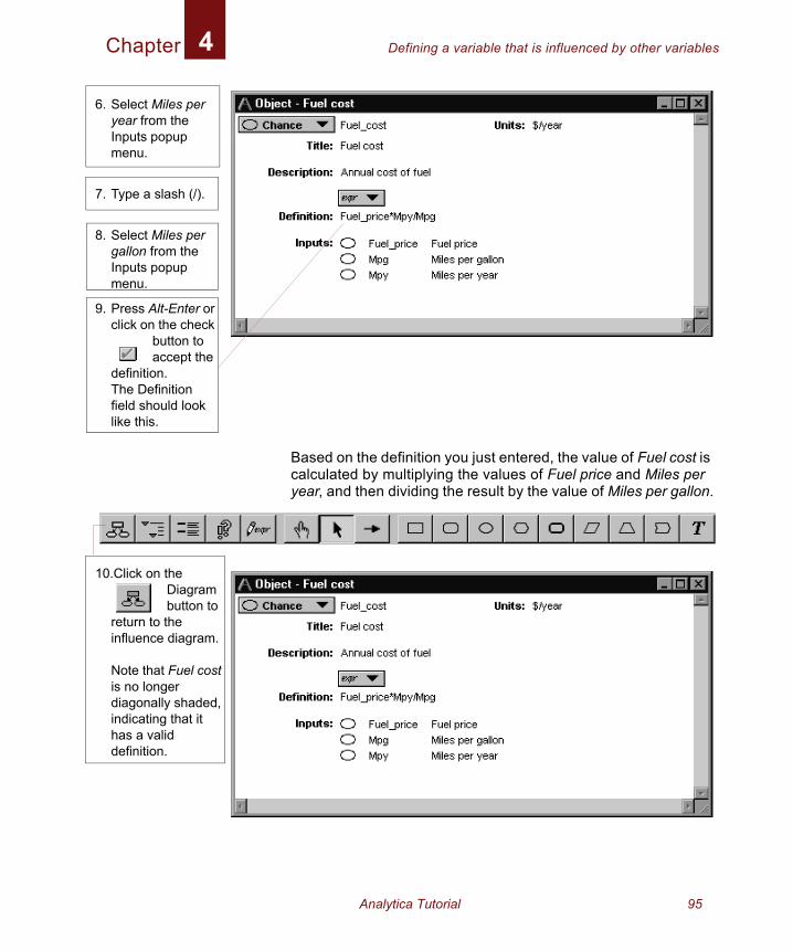
Chapter Defining a variable that is influenced by other variables4
Based on the definition you just entered, the value of Fuel cost is calculated by multiplying the values of Fuel price and Miles per year, and then dividing the result by the value of Miles per gallon.
6. Select Miles per year from the Inputs popup menu.
7. Type a slash (/).
8. Select Miles per gallon from the Inputs popup menu.
9. Press Alt-Enter or click on the check
button to accept the
definition.The Definition field should look like this.
10.Click on the Diagram button to
return to the influence diagram.
Note that Fuel cost is no longer diagonally shaded, indicating that it has a valid definition.
Analytica Tutorial 95
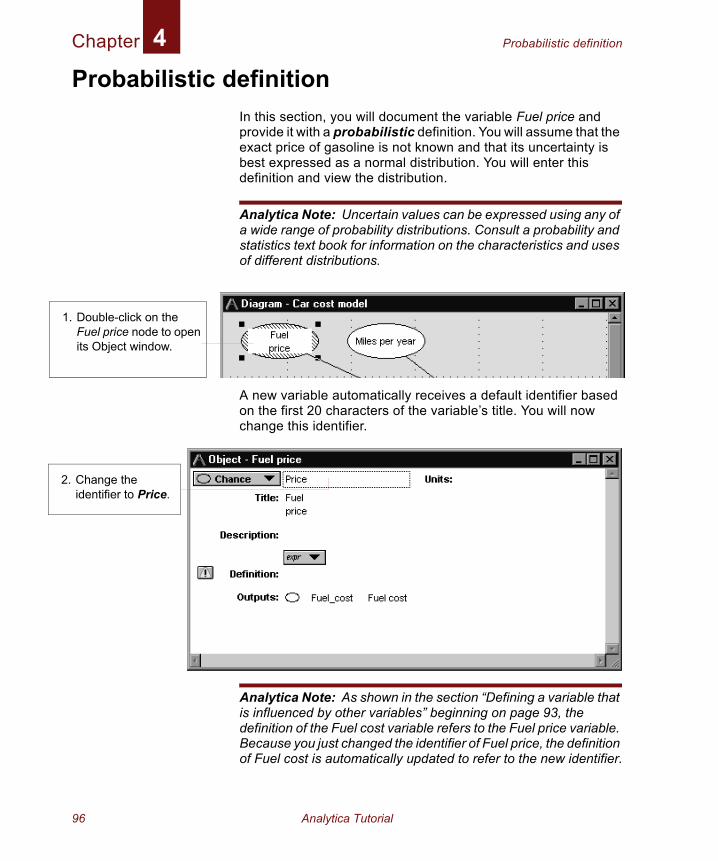
Chapter Probabilistic definition4
Probabilistic definitionIn this section, you will document the variable Fuel price and provide it with a probabilistic definition. You will assume that the exact price of gasoline is not known and that its uncertainty is best expressed as a normal distribution. You will enter this definition and view the distribution.
Analytica Note: Uncertain values can be expressed using any of a wide range of probability distributions. Consult a probability and statistics text book for information on the characteristics and uses of different distributions.
A new variable automatically receives a default identifier based on the first 20 characters of the variable’s title. You will now change this identifier.
Analytica Note: As shown in the section “Defining a variable that is influenced by other variables” beginning on page 93, the definition of the Fuel cost variable refers to the Fuel price variable. Because you just changed the identifier of Fuel price, the definition of Fuel cost is automatically updated to refer to the new identifier.
1. Double-click on the Fuel price node to open its Object window.
2. Change the identifier to Price.
96 Analytica Tutorial
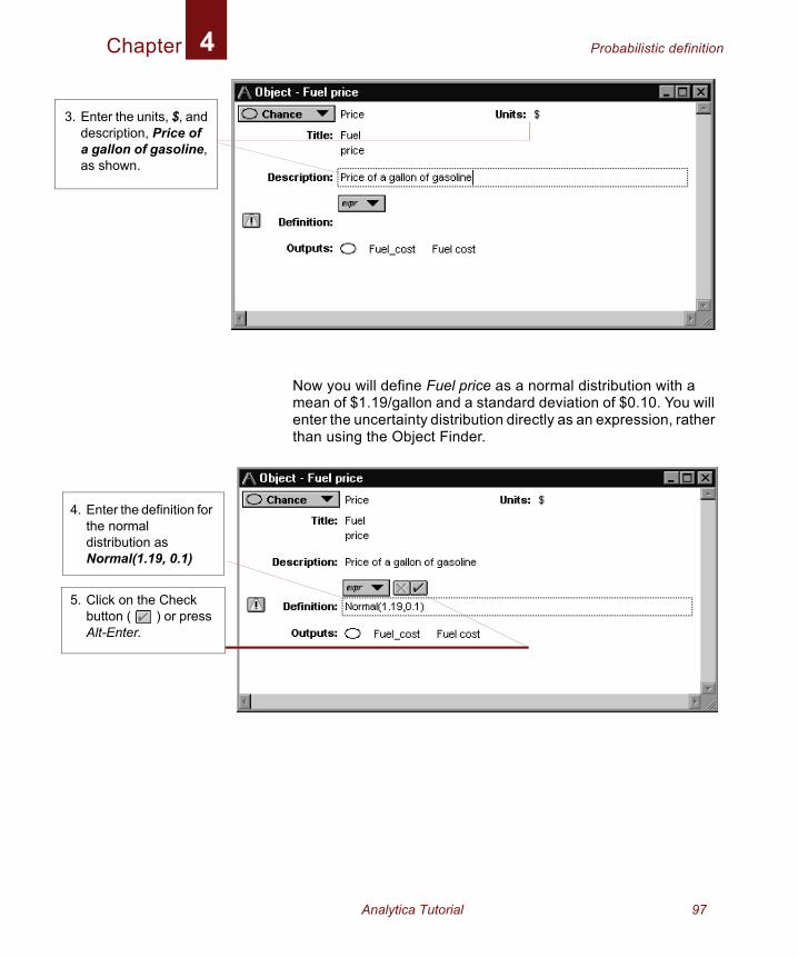
Chapter Probabilistic definition4
3. Endea gas
4. EthdN
5. CbA
Now you will define Fuel price as a normal distribution with a mean of $1.19/gallon and a standard deviation of $0.10. You will enter the uncertainty distribution directly as an expression, rather than using the Object Finder.
ter the units, $, and scription, Price of allon of gasoline,
shown.
nter the definition for e normal
istribution as ormal(1.19, 0.1)
lick on the Check utton ( ) or press lt-Enter.
Analytica Tutorial 97
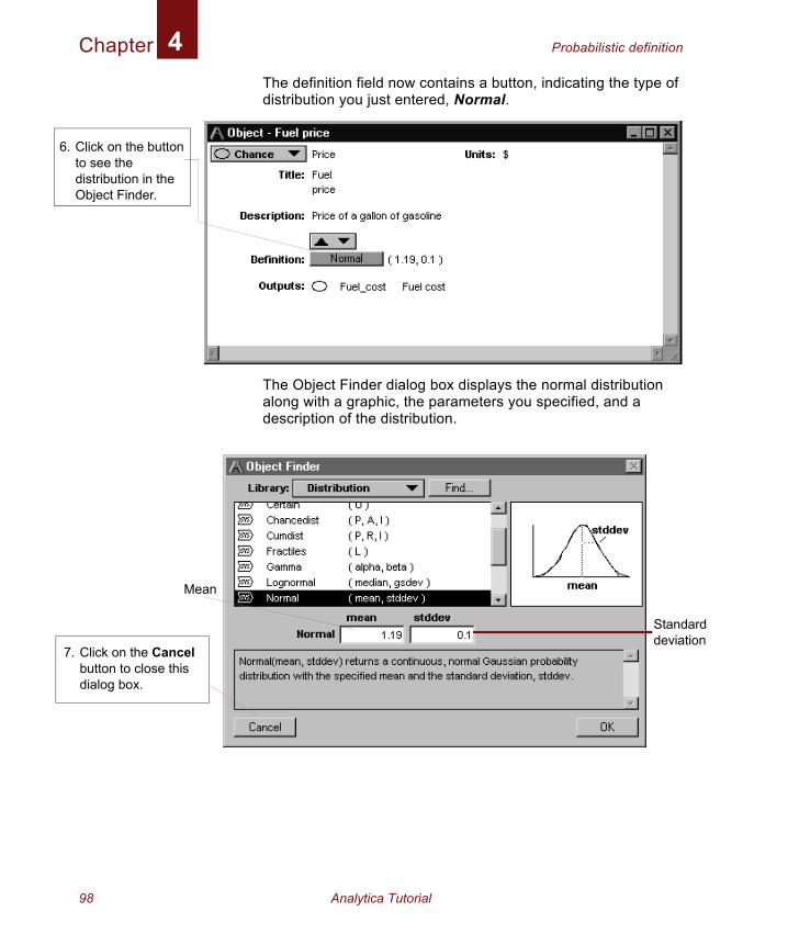
Chapter Probabilistic definition4
6
7
dn
The definition field now contains a button, indicating the type of distribution you just entered, Normal.
The Object Finder dialog box displays the normal distribution along with a graphic, the parameters you specified, and a description of the distribution.
. Click on the button to see the distribution in the Object Finder.
. Click on the Cancel button to close this dialog box.
Standardeviatio
Mean
98 Analytica Tutorial
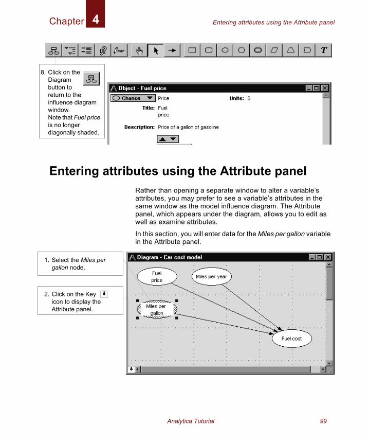
Chapter Entering attributes using the Attribute panel4
8
Entering attributes using the Attribute panelRather than opening a separate window to alter a variable’s attributes, you may prefer to see a variable’s attributes in the same window as the model influence diagram. The Attribute panel, which appears under the diagram, allows you to edit as well as examine attributes.
In this section, you will enter data for the Miles per gallon variable in the Attribute panel.
. Click on the Diagram button to return to the influence diagram window.Note that Fuel price is no longer diagonally shaded.
1. Select the Miles per gallon node.
2. Click on the Key icon to display the Attribute panel.
Analytica Tutorial 99
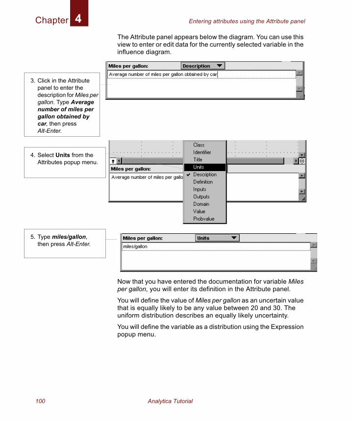
Chapter Entering attributes using the Attribute panel4
The Attribute panel appears below the diagram. You can use this view to enter or edit data for the currently selected variable in the influence diagram.Now that you have entered the documentation for variable Miles per gallon, you will enter its definition in the Attribute panel.
You will define the value of Miles per gallon as an uncertain value that is equally likely to be any value between 20 and 30. The uniform distribution describes an equally likely uncertainty.
You will define the variable as a distribution using the Expression popup menu.
3. Click in the Attribute panel to enter the description for Miles per gallon. Type Average number of miles per gallon obtained by car, then press Alt-Enter.
4. Select Units from the Attributes popup menu.
5. Type miles/gallon, then press Alt-Enter.
100 Analytica Tutorial
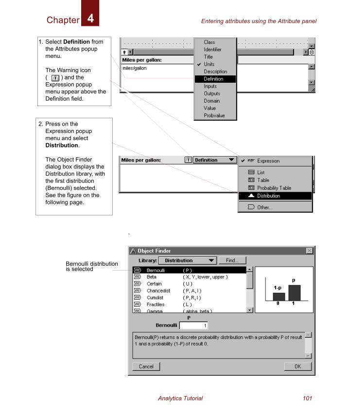
Chapter Entering attributes using the Attribute panel4
1
2
.
. Select Definition from the Attributes popup menu.
The Warning icon ( ) and the Expression popup menu appear above the Definition field.
. Press on the Expression popup menu and select Distribution.
The Object Finder dialog box displays the Distribution library, with the first distribution (Bernoulli) selected. See the figure on the following page.
Bernoulli distribution is selected
Analytica Tutorial 101
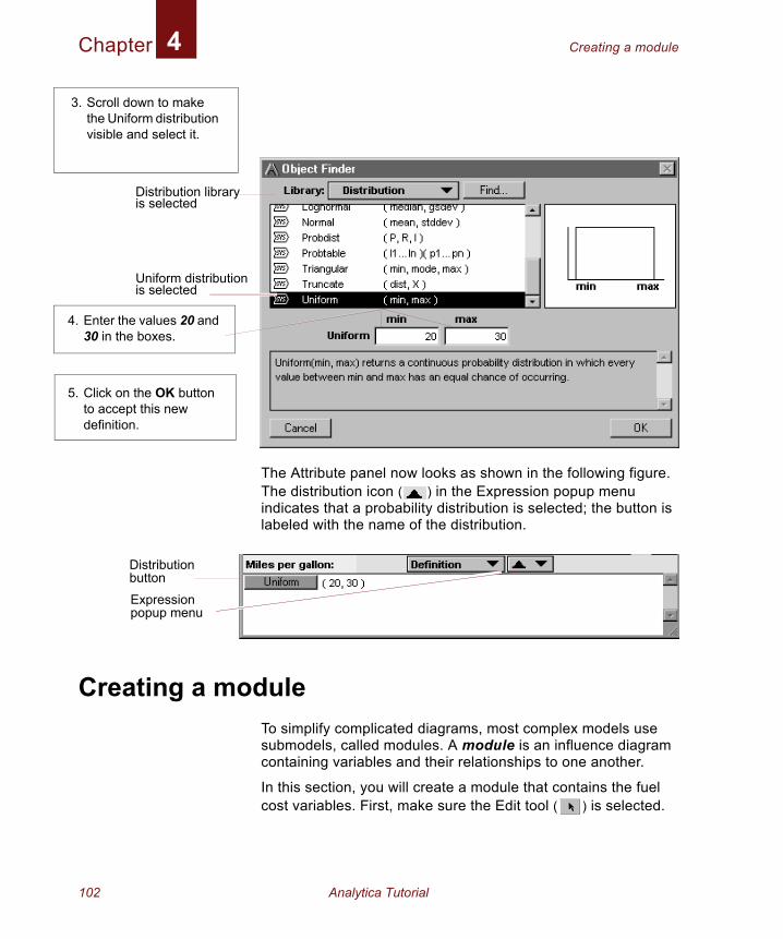
Chapter Creating a module4
The Attribute panel now looks as shown in the following figure. The distribution icon ( ) in the Expression popup menu indicates that a probability distribution is selected; the button is labeled with the name of the distribution.
Creating a moduleTo simplify complicated diagrams, most complex models use submodels, called modules. A module is an influence diagram containing variables and their relationships to one another.
In this section, you will create a module that contains the fuel cost variables. First, make sure the Edit tool ( ) is selected.
4. Enter the values 20 and 30 in the boxes.
5. Click on the OK button to accept this new definition.
Distribution library is selected
Uniform distribution is selected
3. Scroll down to make the Uniform distribution visible and select it.
Distribution buttonExpression popup menu
102 Analytica Tutorial
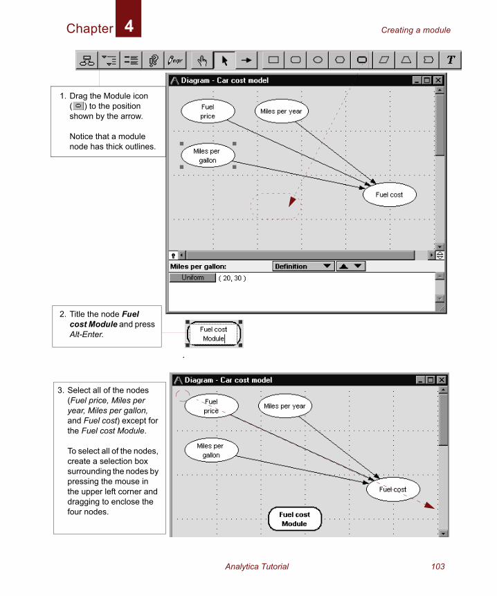
Chapter Creating a module4
3
.
1. Drag the Module icon ( ) to the position shown by the arrow.
Notice that a module node has thick outlines.
2. Title the node Fuel cost Module and press Alt-Enter.
. Select all of the nodes (Fuel price, Miles per year, Miles per gallon, and Fuel cost) except for the Fuel cost Module.
To select all of the nodes, create a selection box surrounding the nodes by pressing the mouse in the upper left corner and dragging to enclose the four nodes.
Analytica Tutorial 103
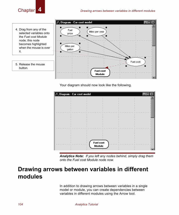
Chapter Drawing arrows between variables in different modules4
Your diagram should now look like the following.
Analytica Note: If you left any nodes behind, simply drag them onto the Fuel cost Module node now.
Drawing arrows between variables in different modules
In addition to drawing arrows between variables in a single model or module, you can create dependencies between variables in different modules using the Arrow tool.
4. Drag from any of the selected variables onto the Fuel cost Module node; this node becomes highlighted when the mouse is over it.
5. Release the mouse button.
104 Analytica Tutorial
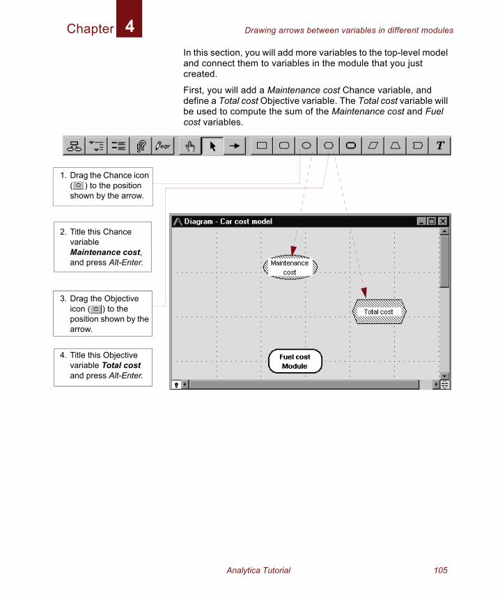
Chapter Drawing arrows between variables in different modules4
In this section, you will add more variables to the top-level model and connect them to variables in the module that you just created.First, you will add a Maintenance cost Chance variable, and define a Total cost Objective variable. The Total cost variable will be used to compute the sum of the Maintenance cost and Fuel cost variables.
1. Drag the Chance icon ( ) to the position shown by the arrow.
2. Title this Chance variable Maintenance cost, and press Alt-Enter.
3. Drag the Objective icon ( ) to the position shown by the arrow.
4. Title this Objective variable Total cost and press Alt-Enter.
Analytica Tutorial 105
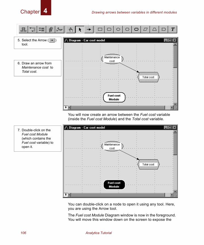
Chapter Drawing arrows between variables in different modules4
You will now create an arrow between the Fuel cost variable (inside the Fuel cost Module) and the Total cost variable.
You can double-click on a node to open it using any tool. Here, you are using the Arrow tool.
The Fuel cost Module Diagram window is now in the foreground. You will move this window down on the screen to expose the
5. Select the Arrow ( ) tool.
6. Draw an arrow from Maintenance cost to Total cost.
7. Double-click on the Fuel cost Module (which contains the Fuel cost variable) to open it.
106 Analytica Tutorial
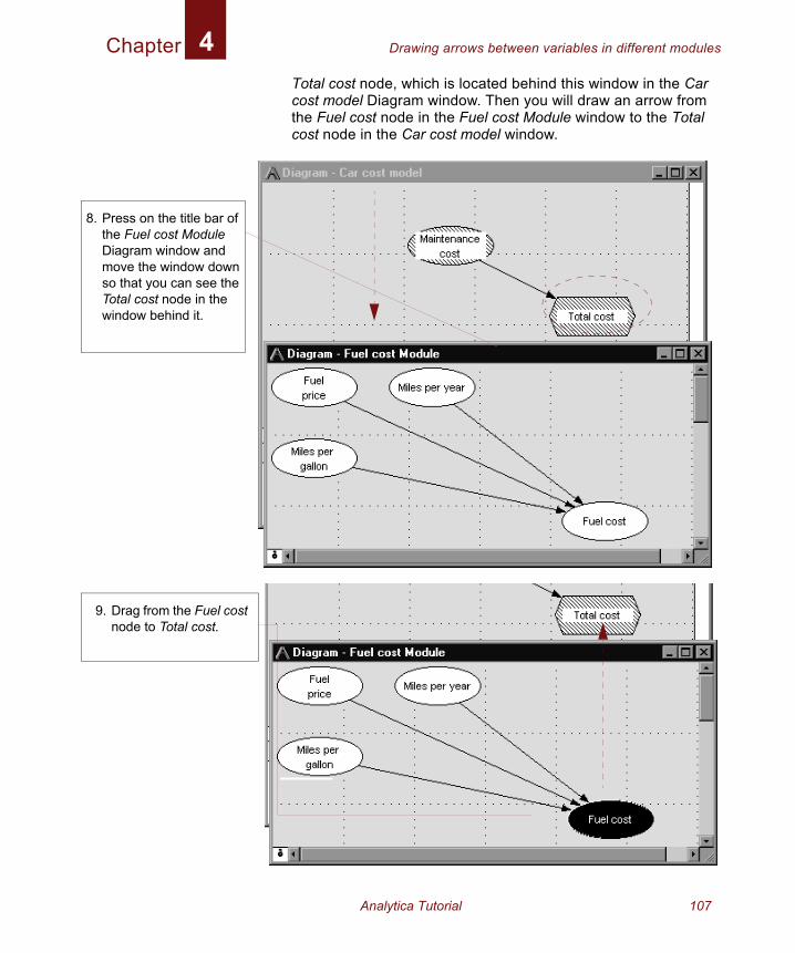
Chapter Drawing arrows between variables in different modules4
8
Total cost node, which is located behind this window in the Car cost model Diagram window. Then you will draw an arrow from the Fuel cost node in the Fuel cost Module window to the Total cost node in the Car cost model window.
. Press on the title bar of the Fuel cost Module Diagram window and move the window down so that you can see the Total cost node in the window behind it.
9. Drag from the Fuel cost node to Total cost.
Analytica Tutorial 107
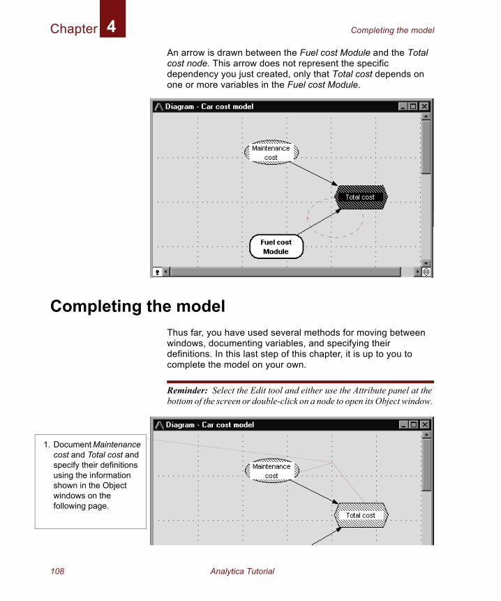
Chapter Completing the model4
An arrow is drawn between the Fuel cost Module and the Total cost node. This arrow does not represent the specific dependency you just created, only that Total cost depends on one or more variables in the Fuel cost Module.Completing the modelThus far, you have used several methods for moving between windows, documenting variables, and specifying their definitions. In this last step of this chapter, it is up to you to complete the model on your own.
Reminder: Select the Edit tool and either use the Attribute panel at the bottom of the screen or double-click on a node to open its Object window.
1. Document Maintenance cost and Total cost and specify their definitions using the information shown in the Object windows on the following page.
108 Analytica Tutorial
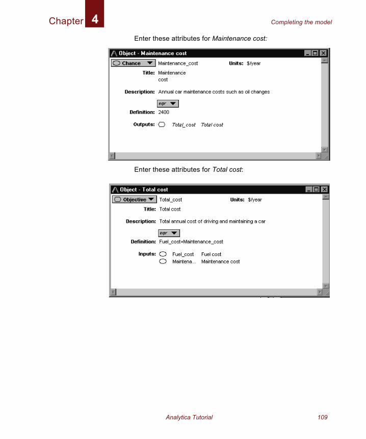
Chapter Completing the model4
Enter these attributes for Maintenance cost:Enter these attributes for Total cost:
Analytica Tutorial 109
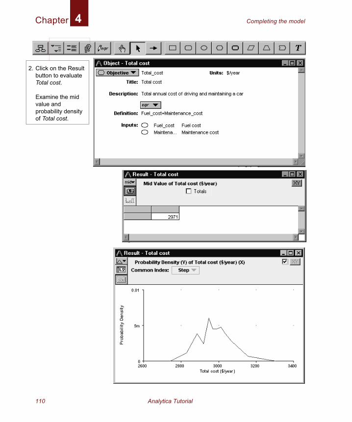
Chapter Completing the model4
2
. Click on the Result button to evaluate Total cost.Examine the mid value and probability density of Total cost.
110 Analytica Tutorial
Chapter Creating the Car Cost model: Summary4
Creating the Car Cost model: SummaryIn this chapter, you have:
• created a model
• documented and defined variables
• created a module
• drawn arrows between variables in the same module and in different modules
In the next chapter, you will extend the Car Cost model to include tables of data.
Saving your model and quittingAfter you have created part or all of a model, you should save it. Because you previously saved your model, it will be saved with the name you gave it.
Close the Attribute panel by clicking on the key ( ).
You may quit Analytica at this point. See “Quitting Analytica” on page 28.
Analytica Tutorial 111

Chapter Saving your model and quitting4
112 Analytica Tutorial

Chapter 5
Creating Arrays (Tables)

In this Chapter
This chapter shows you how to:
• Define index variables
• Define a table and select its indexes
• Define other variables using the same indexes
• View the results of table calculations
• Combine results from a table using the Sum function
Chapter 5: Creating Arrays (Tables)Using the Car Cost model created in the previous chapter, you will create tables, edit their size and dimensions, and compute the results.
An array is a collection of values that can be viewed as one or more spreadsheet-like tables. These terms may be used interchangeably for one or two-dimensional arrays (tables). If an array has more than two dimensions, you must view it as a set of two-dimensional tables. With Analytica's Intelligent Arrays, you can define a variable as an array with as many as fifteen dimensions. You can then use that variable in calculations as easily as if it had been defined as a single number.
The Car Cost model that you saved should be located in the Analytica folder on your hard disk. If you cannot find it, a copy of the Car Cost model is provided in the Tutorial folder, inside the Analytica folder on your hard disk.
Creating an index variableSuppose you own two cars and wish to evaluate the annual costs of each one at the same time. Each car you own has a different value for Miles per gallon and Maintenance cost. Using tables and indexes, you can assign miles per gallon and maintenance costs for each car type and calculate the total costs of each one as simply as calculating the total costs of one car.
In this section you will create and define an index variable, Car type, to distinguish the different cars.
Index variables identify every dimension of multidimensional variables; it’s usually best to plan for and create the indexes before defining the arrays.
First, make sure the Edit tool ( ) is selected.
Analytica Tutorial 115
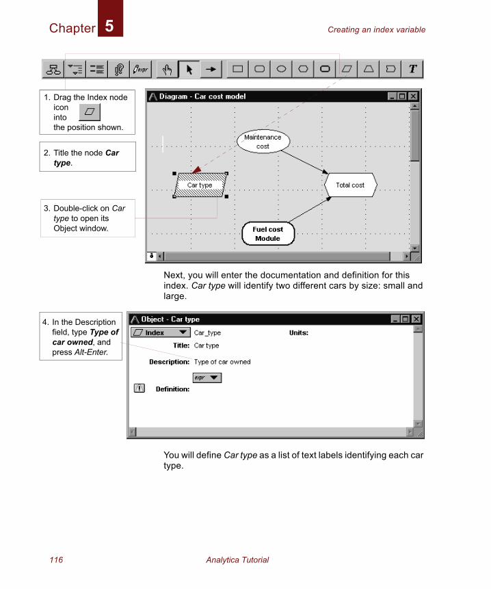
Chapter Creating an index variable5
Next, you will enter the documentation and definition for this index. Car type will identify two different cars by size: small and large.
You will define Car type as a list of text labels identifying each car type.
1. Drag the Index node icon into the position shown.
2. Title the node Car type.
3. Double-click on Car type to open its Object window.
4. In the Description field, type Type of car owned, and press Alt-Enter.
116 Analytica Tutorial
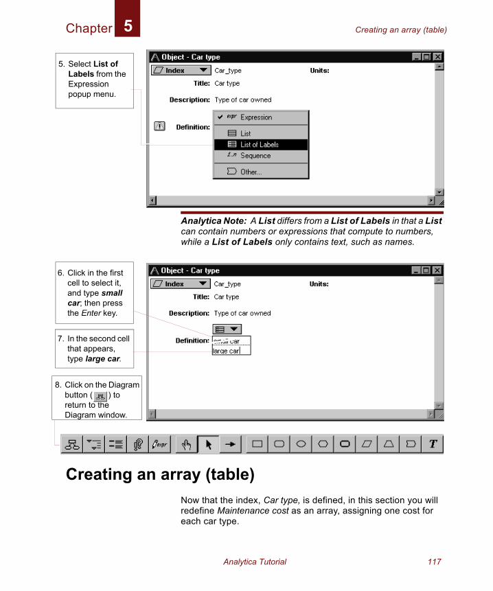
Chapter Creating an array (table)5
8
Analytica Note: A List differs from a List of Labels in that a List can contain numbers or expressions that compute to numbers, while a List of Labels only contains text, such as names.
Creating an array (table)Now that the index, Car type, is defined, in this section you will redefine Maintenance cost as an array, assigning one cost for each car type.
5. Select List of Labels from the Expression popup menu.
6. Click in the first cell to select it, and type small car; then press the Enter key.
7. In the second cell that appears, type large car.
. Click on the Diagram button ( ) to return to the Diagram window.
Analytica Tutorial 117
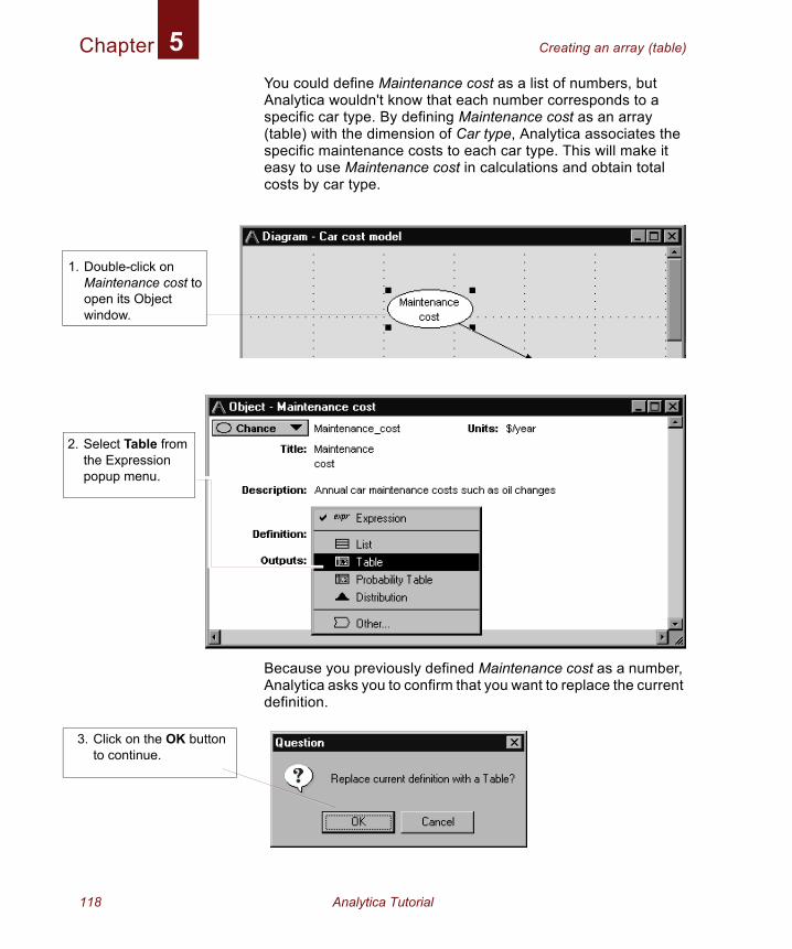
Chapter Creating an array (table)5
You could define Maintenance cost as a list of numbers, but Analytica wouldn't know that each number corresponds to a specific car type. By defining Maintenance cost as an array (table) with the dimension of Car type, Analytica associates the specific maintenance costs to each car type. This will make it easy to use Maintenance cost in calculations and obtain total costs by car type.Because you previously defined Maintenance cost as a number, Analytica asks you to confirm that you want to replace the current definition.
1. Double-click on Maintenance cost to open its Object window.
2. Select Table from the Expression popup menu.
3. Click on the OK button to continue.
118 Analytica Tutorial
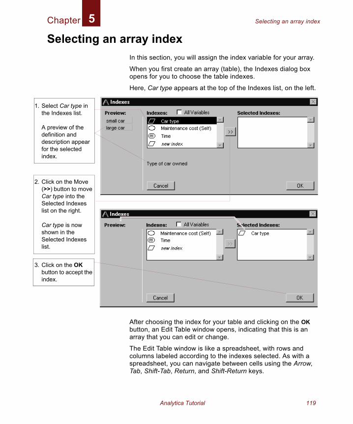
Chapter Selecting an array index5
1.
2.
3.
Selecting an array indexIn this section, you will assign the index variable for your array.
When you first create an array (table), the Indexes dialog box opens for you to choose the table indexes.
Here, Car type appears at the top of the Indexes list, on the left.
After choosing the index for your table and clicking on the OK button, an Edit Table window opens, indicating that this is an array that you can edit or change.
The Edit Table window is like a spreadsheet, with rows and columns labeled according to the indexes selected. As with a spreadsheet, you can navigate between cells using the Arrow, Tab, Shift-Tab, Return, and Shift-Return keys.
Select Car type in the Indexes list.
A preview of the definition and description appear for the selected index.
Click on the Move (>>) button to move Car type into the Selected Indexes list on the right.
Car type is now shown in the Selected Indexes list.
Click on the OK button to accept the index.
Analytica Tutorial 119
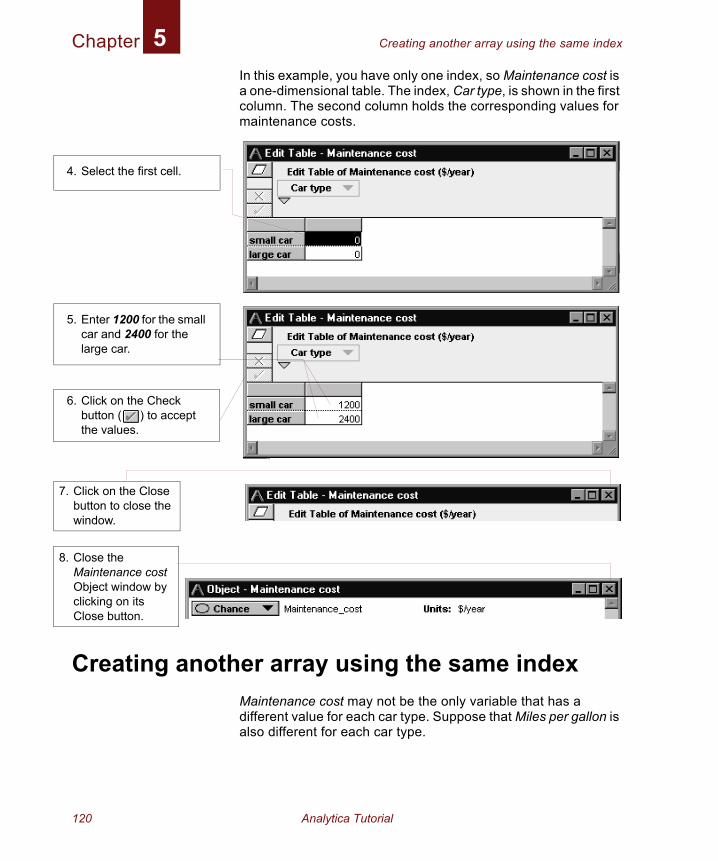
Chapter Creating another array using the same index5
7
8
In this example, you have only one index, so Maintenance cost is a one-dimensional table. The index, Car type, is shown in the first column. The second column holds the corresponding values for maintenance costs.
Creating another array using the same indexMaintenance cost may not be the only variable that has a different value for each car type. Suppose that Miles per gallon is also different for each car type.
4. Select the first cell.
5. Enter 1200 for the small car and 2400 for the large car.
6. Click on the Check button ( ) to accept the values.
. Click on the Close button to close the window.
. Close the Maintenance cost Object window by clicking on its Close button.
120 Analytica Tutorial
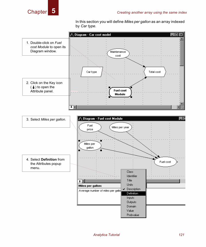
Chapter Creating another array using the same index5
In this section you will define Miles per gallon as an array indexed by Car type.1. Double-click on Fuel cost Module to open its Diagram window.
2. Click on the Key icon ( ) to open the Attribute panel.
3. Select Miles per gallon.
4. Select Definition from the Attributes popup menu.
Analytica Tutorial 121
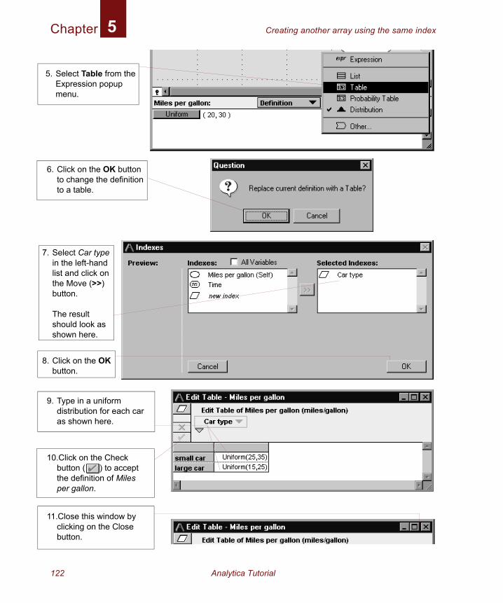
Chapter Creating another array using the same index5
5. Select Table from the Expression popup menu.
6. Click on the OK button to change the definition to a table.
7. Select Car type in the left-hand list and click on the Move (>>) button.
The result should look as shown here.
8. Click on the OK button.
9. Type in a uniform distribution for each car as shown here.
10.Click on the Check button ( ) to accept the definition of Miles per gallon.
11.Close this window by clicking on the Close button.
122 Analytica Tutorial
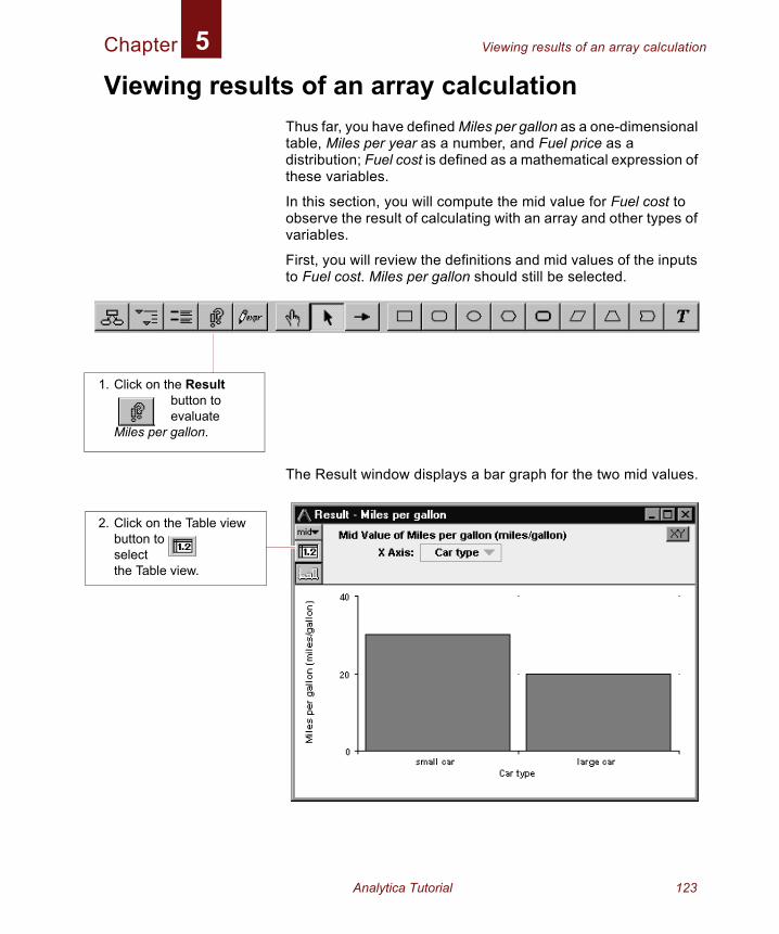
Chapter Viewing results of an array calculation5
Viewing results of an array calculationThus far, you have defined Miles per gallon as a one-dimensional table, Miles per year as a number, and Fuel price as a distribution; Fuel cost is defined as a mathematical expression of these variables.
In this section, you will compute the mid value for Fuel cost to observe the result of calculating with an array and other types of variables.
First, you will review the definitions and mid values of the inputs to Fuel cost. Miles per gallon should still be selected.
The Result window displays a bar graph for the two mid values.
1. Click on the Result button to evaluate
Miles per gallon.
2. Click on the Table view button to select the Table view.
Analytica Tutorial 123
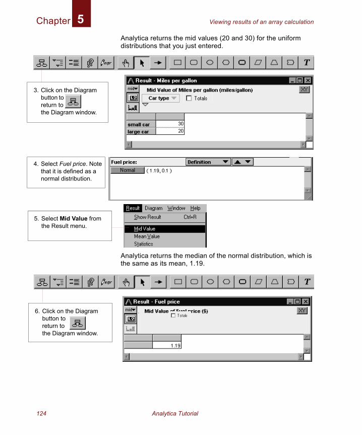
Chapter Viewing results of an array calculation5
Analytica returns the mid values (20 and 30) for the uniform distributions that you just entered.Analytica returns the median of the normal distribution, which is the same as its mean, 1.19.
3. Click on the Diagram button to return to the Diagram window.
4. Select Fuel price. Note that it is defined as a normal distribution.
5. Select Mid Value from the Result menu.
6. Click on the Diagram button to return to the Diagram window.
124 Analytica Tutorial
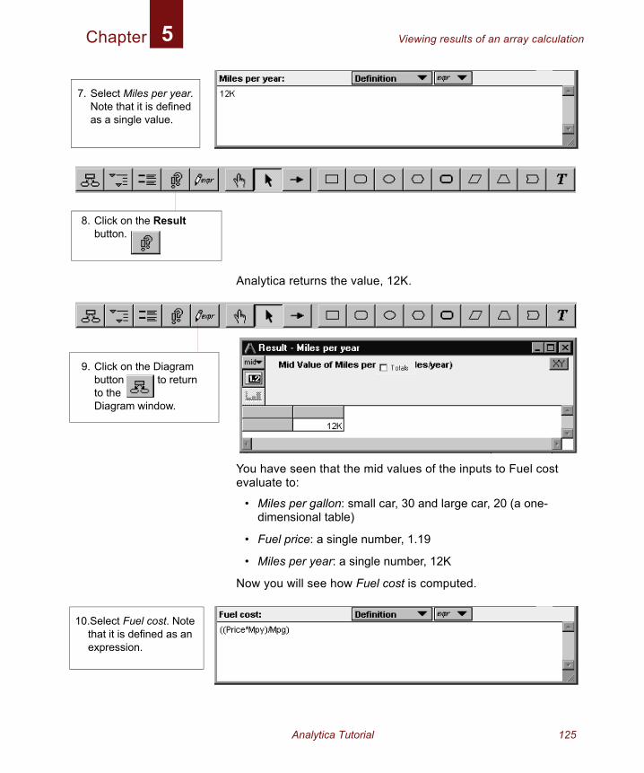
Chapter Viewing results of an array calculation5
1
Analytica returns the value, 12K.
You have seen that the mid values of the inputs to Fuel cost evaluate to:
• Miles per gallon: small car, 30 and large car, 20 (a one-dimensional table)
• Fuel price: a single number, 1.19
• Miles per year: a single number, 12K
Now you will see how Fuel cost is computed.
7. Select Miles per year. Note that it is defined as a single value.
8. Click on the Result button.
9. Click on the Diagram button to returnto theDiagram window.
0.Select Fuel cost. Note that it is defined as an expression.
Analytica Tutorial 125
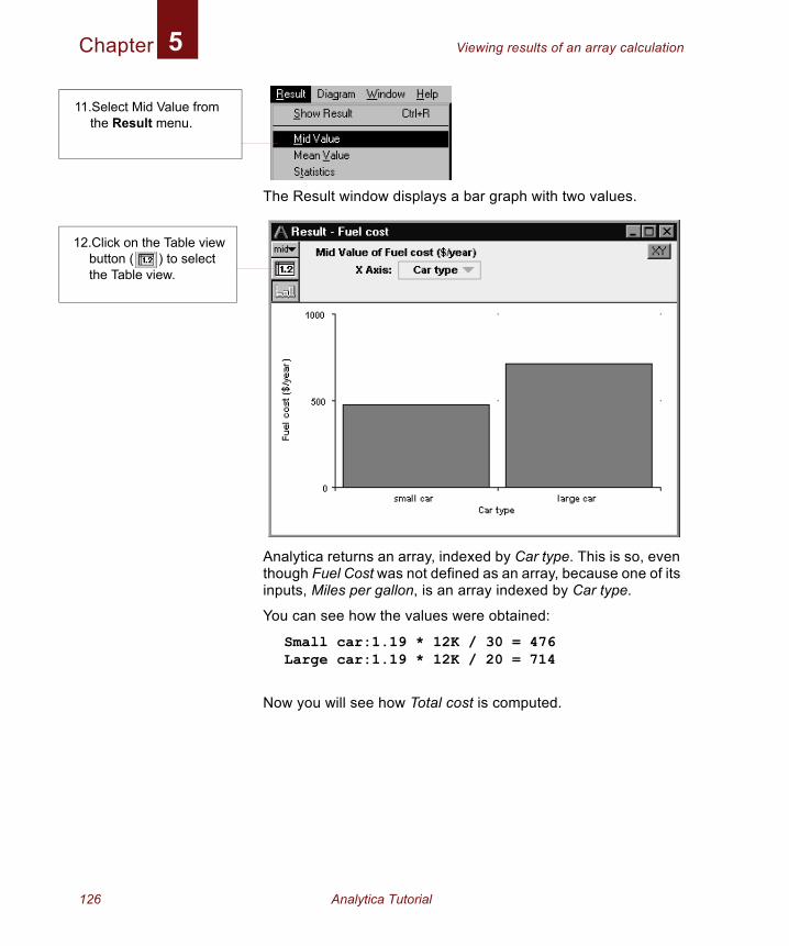
Chapter Viewing results of an array calculation5
The Result window displays a bar graph with two values.
Analytica returns an array, indexed by Car type. This is so, even though Fuel Cost was not defined as an array, because one of its inputs, Miles per gallon, is an array indexed by Car type.
You can see how the values were obtained:
Small car:1.19 * 12K / 30 = 476Large car:1.19 * 12K / 20 = 714
Now you will see how Total cost is computed.
11.Select Mid Value from the Result menu.
12.Click on the Table view button ( ) to select the Table view.
126 Analytica Tutorial
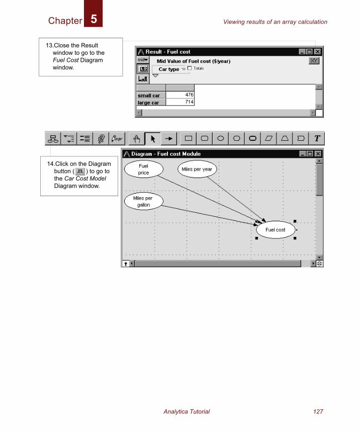
Chapter Viewing results of an array calculation5
13.Close the Result window to go to the Fuel Cost Diagram window.
14.Click on the Diagram button ( ) to go to the Car Cost Model Diagram window.
Analytica Tutorial 127
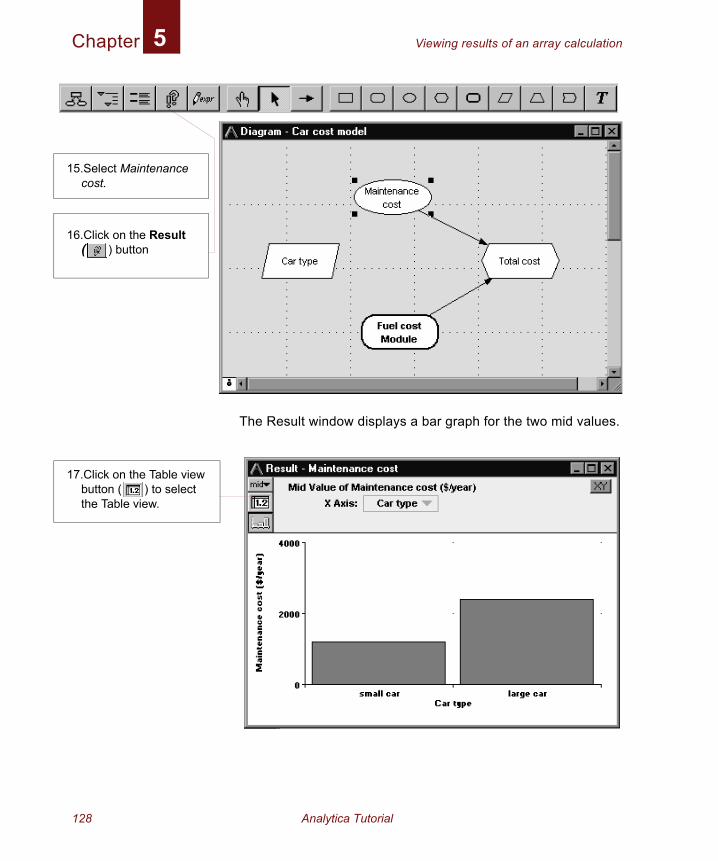
Chapter Viewing results of an array calculation5
The Result window displays a bar graph for the two mid values.
15.Select Maintenance cost.
16.Click on the Result ( ) button
17.Click on the Table view button ( ) to select the Table view.
128 Analytica Tutorial
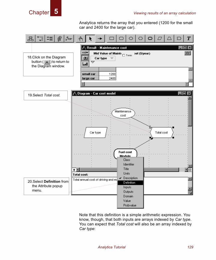
Chapter Viewing results of an array calculation5
Analytica returns the array that you entered (1200 for the small car and 2400 for the large car).Note that this definition is a simple arithmetic expression. You know, though, that both inputs are arrays indexed by Car type. You can expect that Total cost will also be an array indexed by Car type:
18.Click on the Diagram button ( ) to return to the Diagram window.
19.Select Total cost.
20.Select Definition from the Attribute popup menu.
Analytica Tutorial 129
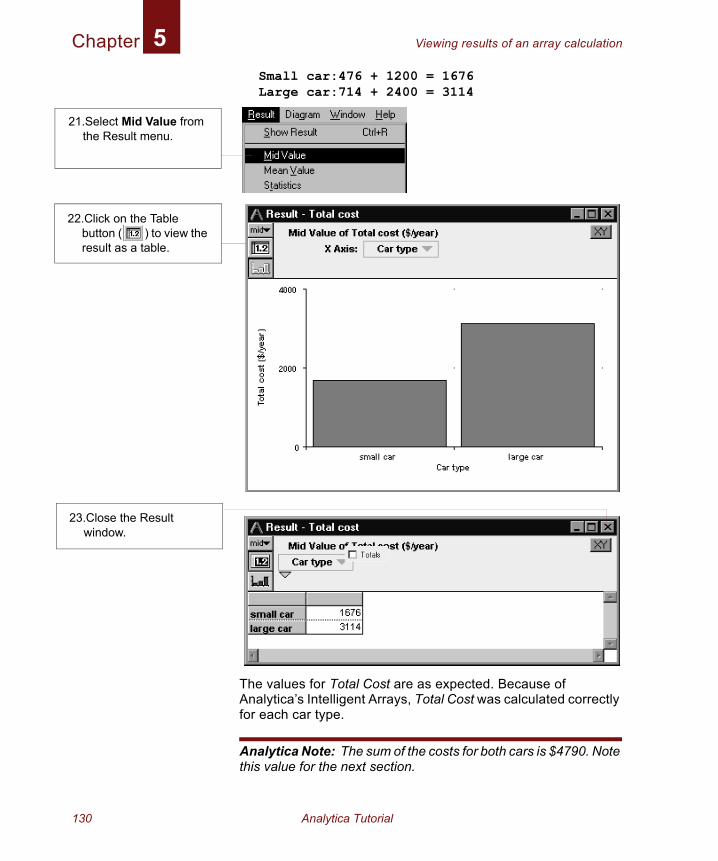
Chapter Viewing results of an array calculation5
Small car:476 + 1200 = 1676Large car:714 + 2400 = 3114The values for Total Cost are as expected. Because of Analytica’s Intelligent Arrays, Total Cost was calculated correctly for each car type.
Analytica Note: The sum of the costs for both cars is $4790. Note this value for the next section.
21.Select Mid Value from the Result menu.
22.Click on the Table button ( ) to view the result as a table.
23.Close the Result window.
130 Analytica Tutorial
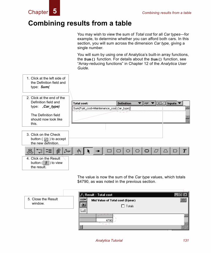
Chapter Combining results from a table5
Combining results from a tableYou may wish to view the sum of Total cost for all Car types—for example, to determine whether you can afford both cars. In this section, you will sum across the dimension Car type, giving a single number.
You will sum by using one of Analytica’s built-in array functions, the Sum() function. For details about the Sum() function, see “Array-reducing functions” in Chapter 12 of the Analytica User Guide.
The value is now the sum of the Car type values, which totals $4790, as was noted in the previous section.
1. Click at the left side of the Definition field and type: Sum(
2. Click at the end of the Definition field and type: ,Car_type)
The Definition field should now look like this.
3. Click on the Check button ( ) to accept the new definition.
4. Click on the Result button ( ) to view the result.
5. Close the Result window.
Analytica Tutorial 131
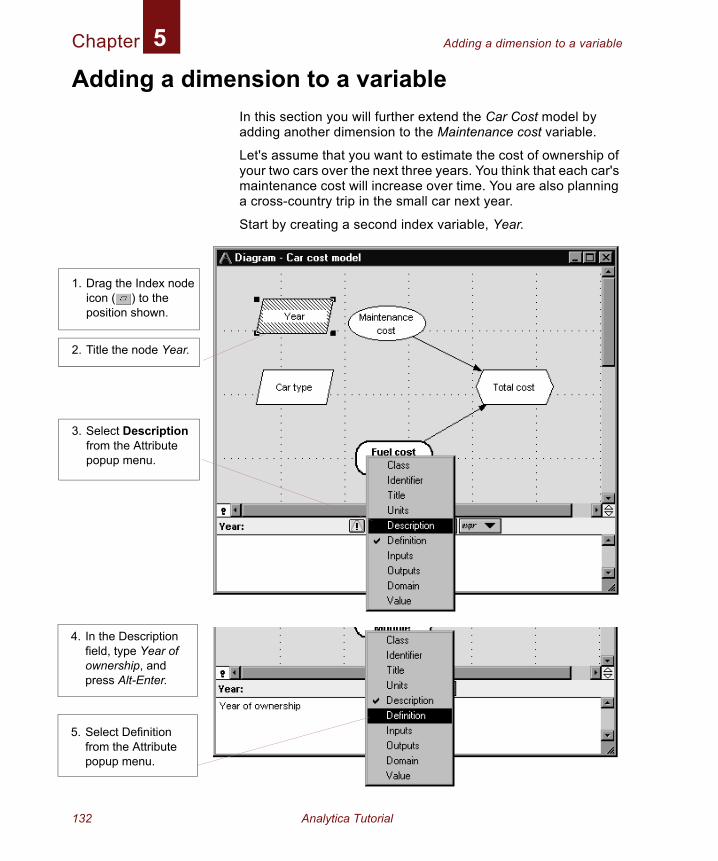
Chapter Adding a dimension to a variable5
Adding a dimension to a variableIn this section you will further extend the Car Cost model by adding another dimension to the Maintenance cost variable.
Let's assume that you want to estimate the cost of ownership of your two cars over the next three years. You think that each car's maintenance cost will increase over time. You are also planning a cross-country trip in the small car next year.
Start by creating a second index variable, Year.
1. Drag the Index node icon ( ) to the position shown.
2. Title the node Year.
3. Select Description from the Attribute popup menu.
4. In the Description field, type Year of ownership, and press Alt-Enter.
5. Select Definition from the Attribute popup menu.
132 Analytica Tutorial
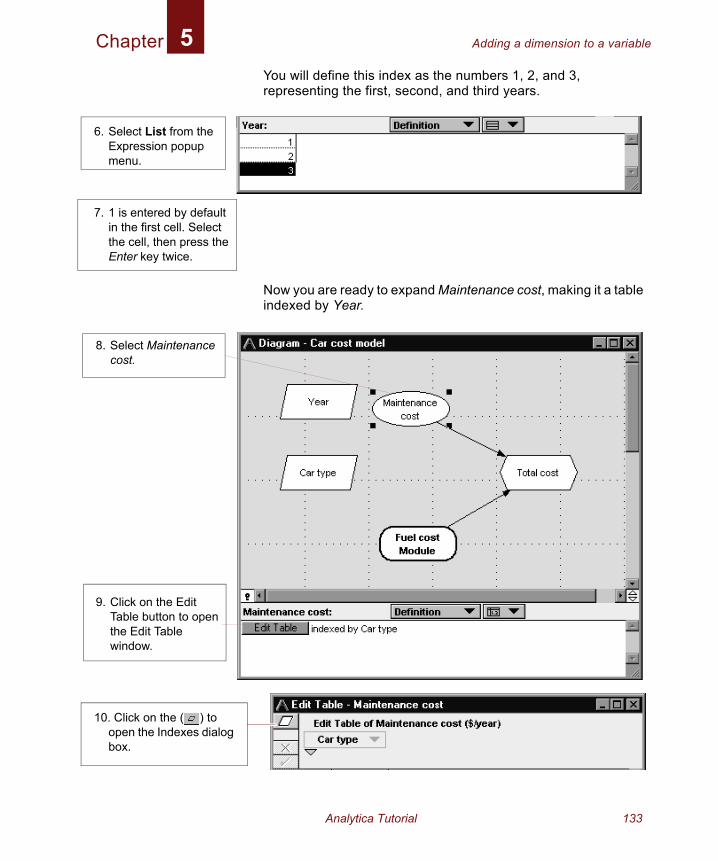
Chapter Adding a dimension to a variable5
You will define this index as the numbers 1, 2, and 3, representing the first, second, and third years.Now you are ready to expand Maintenance cost, making it a table indexed by Year.
6. Select List from the Expression popup menu.
7. 1 is entered by default in the first cell. Select the cell, then press the Enter key twice.
8. Select Maintenance cost.
9. Click on the Edit Table button to open the Edit Table window.
10. Click on the ( ) to open the Indexes dialog box.
Analytica Tutorial 133
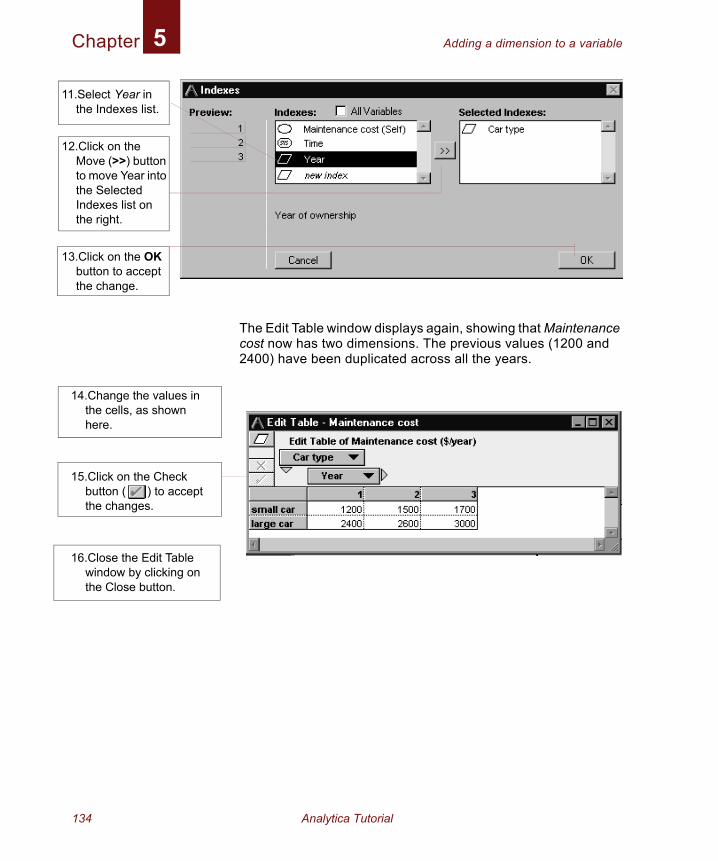
Chapter Adding a dimension to a variable5
The Edit Table window displays again, showing that Maintenance cost now has two dimensions. The previous values (1200 and 2400) have been duplicated across all the years.
11.Select Year in the Indexes list.
12.Click on the Move (>>) button to move Year into the Selected Indexes list on the right.
13.Click on the OK button to accept the change.
14.Change the values in the cells, as shown here.
15.Click on the Check button ( ) to accept the changes.
16.Close the Edit Table window by clicking on the Close button.
134 Analytica Tutorial
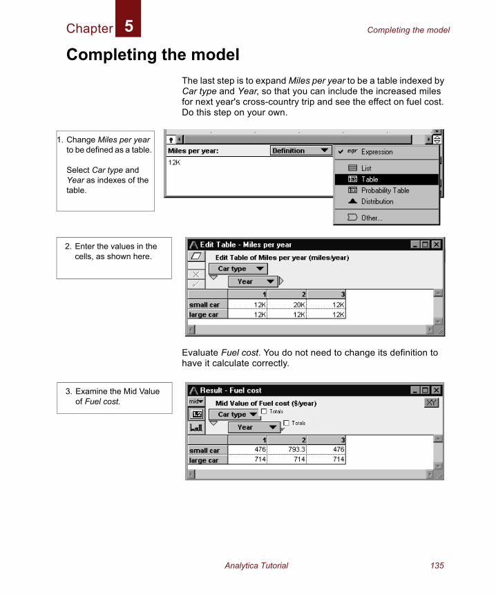
Chapter Completing the model5
1
Completing the modelThe last step is to expand Miles per year to be a table indexed by Car type and Year, so that you can include the increased miles for next year's cross-country trip and see the effect on fuel cost. Do this step on your own.
Evaluate Fuel cost. You do not need to change its definition to have it calculate correctly.
. Change Miles per year to be defined as a table.
Select Car type and Year as indexes of the table.
2. Enter the values in the cells, as shown here.
3. Examine the Mid Value of Fuel cost.
Analytica Tutorial 135
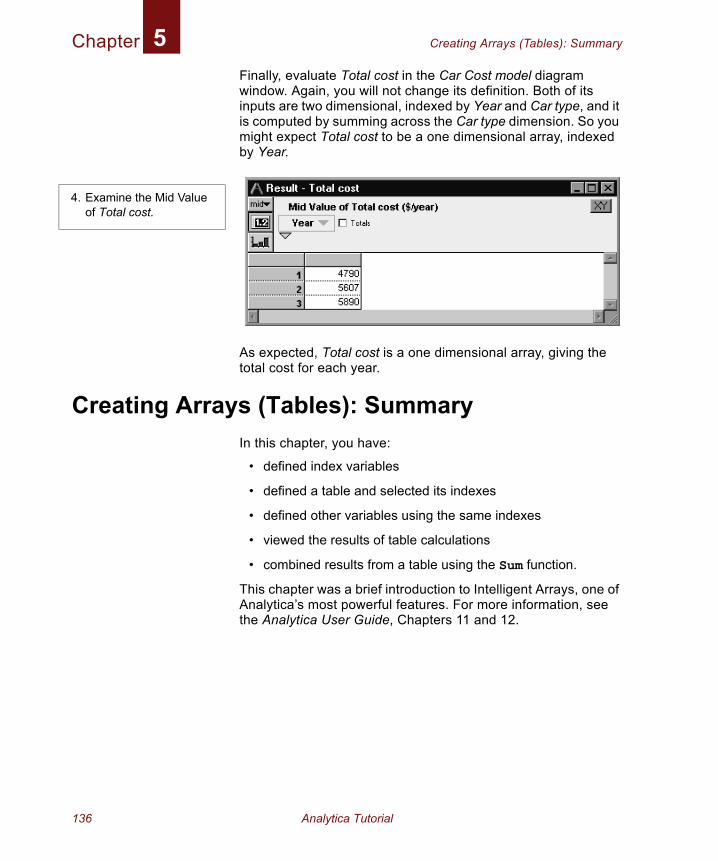
Chapter Creating Arrays (Tables): Summary5
Finally, evaluate Total cost in the Car Cost model diagram window. Again, you will not change its definition. Both of its inputs are two dimensional, indexed by Year and Car type, and it is computed by summing across the Car type dimension. So you might expect Total cost to be a one dimensional array, indexed by Year.As expected, Total cost is a one dimensional array, giving the total cost for each year.
Creating Arrays (Tables): SummaryIn this chapter, you have:
• defined index variables
• defined a table and selected its indexes
• defined other variables using the same indexes
• viewed the results of table calculations
• combined results from a table using the Sum function.
This chapter was a brief introduction to Intelligent Arrays, one of Analytica’s most powerful features. For more information, see the Analytica User Guide, Chapters 11 and 12.
4. Examine the Mid Value of Total cost.
136 Analytica Tutorial

Chapter 6
Creating the Party Problem Model

In this Chapter
This chapter shows you how to:
• Define a variable as a probability table
• Define a variable as a deterministic table
Chapter 6: Creating the Party Problem ModelIn this chapter you will create a new Analytica model called Party Problem. (For information about how to create a new model, see the beginning of Chapter 4, “Creating a Model”.) The Party Problem model illustrates the use of discrete probability distributions.
You should study this chapter if your models will use discrete or conditional probabilities.
In many kinds of models, your variables may be described using probability distributions based on expert judgment or on empirical data. On those occasions when the outcomes are discrete or qualitative (for example, low, medium, or high), you may need to use discrete probability distributions.
In the Party Problem model, the key uncertain variable is weather: it could be sunny or rainy. The weather has an impact on the decision about the location of a party—indoors, on a porch, or outdoors.
Analytica Tutorial 139
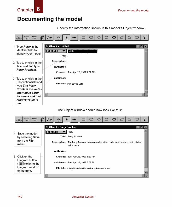
Chapter Documenting the model6
1
2
3
4
5
Documenting the modelSpecify the information shown in this model's Object window.
The Object window should now look like this:
. Type Party in the Identifier field to identify your model.
. Tab to or click in the Title field and type Party Problem.
. Tab to or click in the Description field and type The Party Problem evaluates alternative party locations and their relative value to me.
. Save the model by selecting Save from the File menu.
. Click on the Diagram button ( ) to bring the Diagram window to the front.
140 Analytica Tutorial
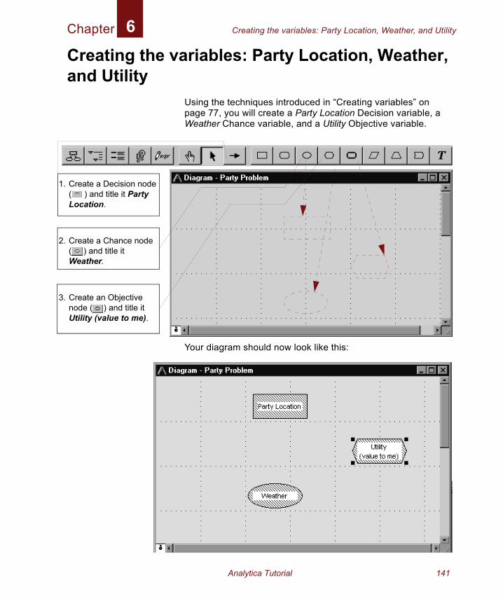
Chapter Creating the variables: Party Location, Weather, and Utility6
Creating the variables: Party Location, Weather, and UtilityUsing the techniques introduced in “Creating variables” on page 77, you will create a Party Location Decision variable, a Weather Chance variable, and a Utility Objective variable.
Your diagram should now look like this:
1. Create a Decision node ( ) and title it Party Location.
2. Create a Chance node ( ) and title it Weather.
3. Create an Objective node ( ) and title it Utility (value to me).
Analytica Tutorial 141
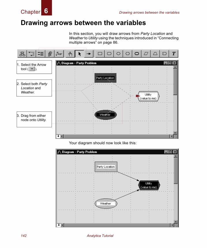
Chapter Drawing arrows between the variables6
1
2
3
Drawing arrows between the variablesIn this section, you will draw arrows from Party Location and Weather to Utility using the techniques introduced in “Connecting multiple arrows” on page 86.
Your diagram should now look like this:
. Select the Arrow tool ( ).
. Select both Party Location and Weather.
. Drag from either node onto Utility.
142 Analytica Tutorial
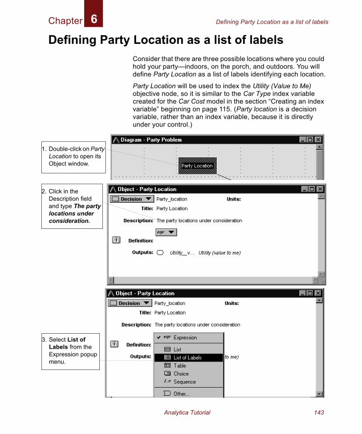
Chapter Defining Party Location as a list of labels6
1
2
3
Defining Party Location as a list of labelsConsider that there are three possible locations where you could hold your party—indoors, on the porch, and outdoors. You will define Party Location as a list of labels identifying each location.
Party Location will be used to index the Utility (Value to Me) objective node, so it is similar to the Car Type index variable created for the Car Cost model in the section “Creating an index variable” beginning on page 115. (Party location is a decision variable, rather than an index variable, because it is directly under your control.)
. Double-click on Party Location to open its Object window.
. Click in the Description field and type The party locations under consideration.
. Select List of Labels from the Expression popup menu.
Analytica Tutorial 143
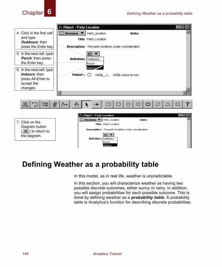
Chapter Defining Weather as a probability table6
4
5
6
7
Defining Weather as a probability tableIn this model, as in real life, weather is unpredictable.
In this section, you will characterize weather as having two possible discrete outcomes, either sunny or rainy. In addition, you will assign probabilities for each possible outcome. This is done by defining weather as a probability table. A probability table is Analytica’s function for describing discrete probabilities.
. Click in the first cell and type Outdoors; then press the Enter key.
. In the next cell, type Porch; then press the Enter key.
. In the next cell, type Indoors; then press Alt-Enter to accept the changes.
. Click on the Diagram button ( ) to return to the diagram.
144 Analytica Tutorial
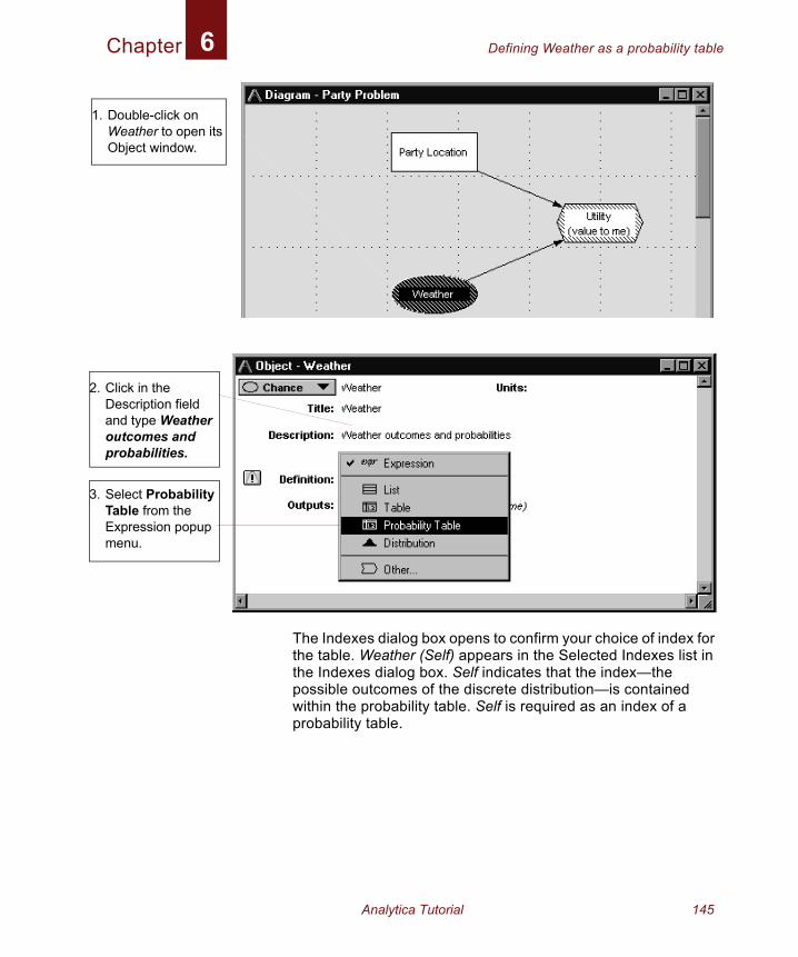
Chapter Defining Weather as a probability table6
1
2
3
The Indexes dialog box opens to confirm your choice of index for the table. Weather (Self) appears in the Selected Indexes list in the Indexes dialog box. Self indicates that the index—the possible outcomes of the discrete distribution—is contained within the probability table. Self is required as an index of a probability table.
. Double-click on Weather to open its Object window.
. Click in the Description field and type Weather outcomes and probabilities.
. Select Probability Table from the Expression popup menu.
Analytica Tutorial 145
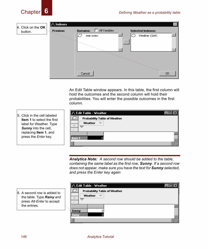
Chapter Defining Weather as a probability table6
4
An Edit Table window appears. In this table, the first column will hold the outcomes and the second column will hold their probabilities. You will enter the possible outcomes in the first column.
Analytica Note: A second row should be added to the table, containing the same label as the first row, Sunny. If a second row does not appear, make sure you have the text for Sunny selected, and press the Enter key again
. Click on the OK button.
5. Click in the cell labeled Item 1 to select the first label for Weather. Type Sunny into the cell, replacing Item 1, and press the Enter key.
6. A second row is added to the table. Type Rainy and press Alt-Enter to accept the entries.
146 Analytica Tutorial
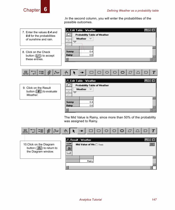
Chapter Defining Weather as a probability table6
.In the second column, you will enter the probabilities of the possible outcomes.The Mid Value is Rainy, since more than 50% of the probability was assigned to Rainy.
7. Enter the values 0.4 and 0.6 for the probabilities of sunshine and rain.
8. Click on the Check button ( ) to accept these entries.
9. Click on the Result button ( ) to evaluate Weather.
10.Click on the Diagram button ( ) to return to the Diagram window.
Analytica Tutorial 147
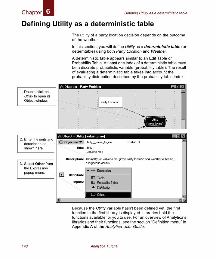
Chapter Defining Utility as a deterministic table6
Defining Utility as a deterministic tableThe utility of a party location decision depends on the outcome of the weather.
In this section, you will define Utility as a deterministic table (or determtable) using both Party Location and Weather.
A deterministic table appears similar to an Edit Table or Probability Table. At least one index of a deterministic table must be a discrete probabilistic variable (probability table). The result of evaluating a deterministic table takes into account the probability distribution described by the probability table index.
Because the Utility variable hasn't been defined yet, the first function in the first library is displayed. Libraries hold the functions available for you to use. For an overview of Analytica’s libraries and their functions, see the section “Definition menu” in Appendix A of the Analytica User Guide.
1. Double-click on Utility to open its Object window.
2. Enter the units and description as shown here.
3. Select Other from the Expression popup menu.
148 Analytica Tutorial
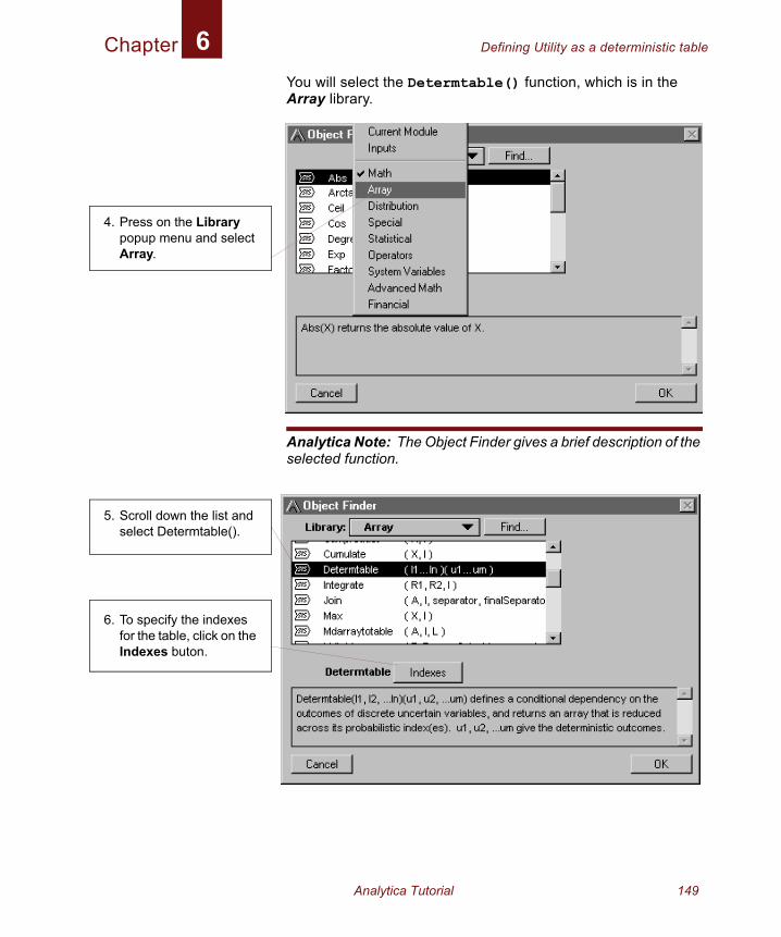
Chapter Defining Utility as a deterministic table6
You will select the Determtable() function, which is in the Array library.Analytica Note: The Object Finder gives a brief description of the selected function.
4. Press on the Library popup menu and select Array.
5. Scroll down the list and select Determtable().
6. To specify the indexes for the table, click on the Indexes buton.
Analytica Tutorial 149
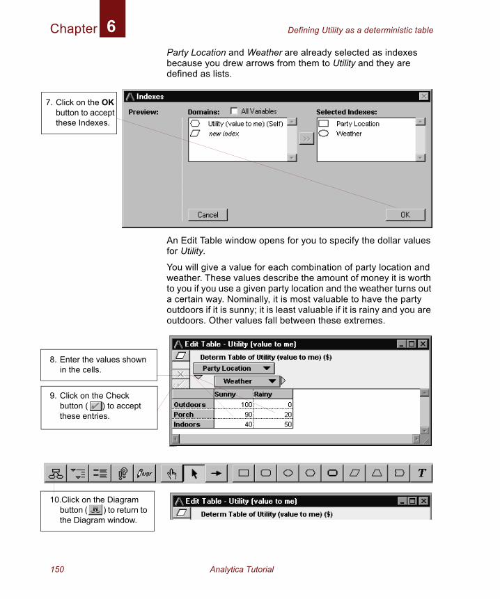
Chapter Defining Utility as a deterministic table6
Party Location and Weather are already selected as indexes because you drew arrows from them to Utility and they are defined as lists.An Edit Table window opens for you to specify the dollar values for Utility.
You will give a value for each combination of party location and weather. These values describe the amount of money it is worth to you if you use a given party location and the weather turns out a certain way. Nominally, it is most valuable to have the party outdoors if it is sunny; it is least valuable if it is rainy and you are outdoors. Other values fall between these extremes.
7. Click on the OK button to accept these Indexes.
8. Enter the values shown in the cells.
9. Click on the Check button ( ) to accept these entries.
10.Click on the Diagram button ( ) to return to the Diagram window.
150 Analytica Tutorial
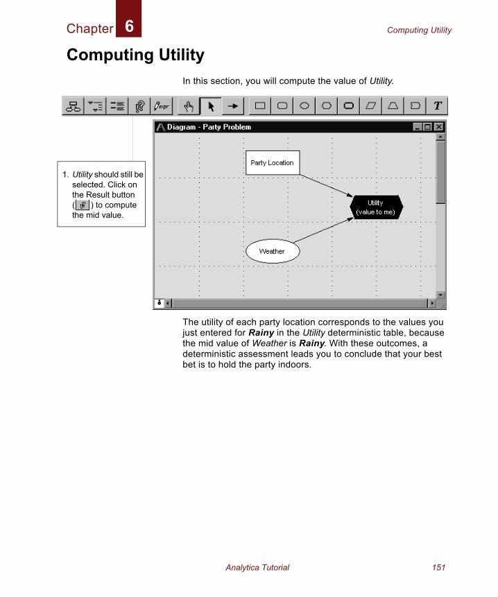
Chapter Computing Utility6
Computing UtilityIn this section, you will compute the value of Utility.
The utility of each party location corresponds to the values you just entered for Rainy in the Utility deterministic table, because the mid value of Weather is Rainy. With these outcomes, a deterministic assessment leads you to conclude that your best bet is to hold the party indoors.
1. Utility should still be selected. Click on the Result button ( ) to compute the mid value.
Analytica Tutorial 151
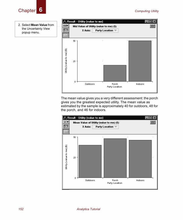
Chapter Computing Utility6
The mean value gives you a very different assessment: the porch gives you the greatest expected utility. The mean value as estimated by the sample is approximately 40 for outdoors, 48 for the porch, and 46 for indoors.
2. Select Mean Value from the Uncertainty View popup menu.
152 Analytica Tutorial
Chapter Computing Utility6
The exact expected utility for each party location can be calculated by multiplying the probabilities of the outcomes by the values of Utility:Outdoors= (100)*0.4 + (0)*0.6= 40Porch = (90)*0.4 + (20)*0.6= 48Indoors= (40)*0.4 + (50)*0.6= 46
Note to those with a background in discrete modeling:Analytica simulates all probability distributions and calculates the expected (mean) value of a distribution by computing the average of the samples. For a discrete distribution, the computed mean converges, with increasing sample size, toward the value obtained by multiplying the probabilities by the discrete outcome values.
Analytica Tutorial 153
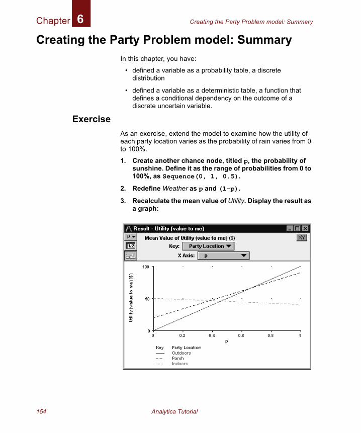
Chapter Creating the Party Problem model: Summary6
Creating the Party Problem model: SummaryIn this chapter, you have:
• defined a variable as a probability table, a discrete distribution
• defined a variable as a deterministic table, a function that defines a conditional dependency on the outcome of a discrete uncertain variable.
ExerciseAs an exercise, extend the model to examine how the utility of each party location varies as the probability of rain varies from 0 to 100%.
1. Create another chance node, titled p, the probability of sunshine. Define it as the range of probabilities from 0 to 100%, as Sequence(0, 1, 0.5).
2. Redefine Weather as p and (1-p).
3. Recalculate the mean value of Utility. Display the result as a graph:
154 Analytica Tutorial

Chapter 7
Creating the Foxes and Hares Model

In this Chapter
This chapter shows you how to:
• Use the Dynamic() function and the system variable Time
• Calculate the results of two nodes simultaneously
• Include variable names in definitions
• Use the Min() and Max() functions
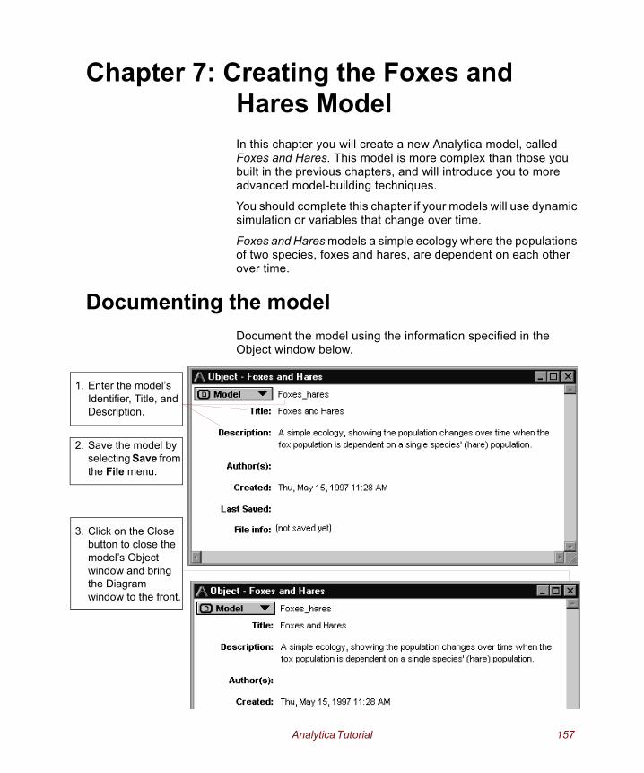
3
Chapter 7: Creating the Foxes and Hares ModelIn this chapter you will create a new Analytica model, called Foxes and Hares. This model is more complex than those you built in the previous chapters, and will introduce you to more advanced model-building techniques.
You should complete this chapter if your models will use dynamic simulation or variables that change over time.
Foxes and Hares models a simple ecology where the populations of two species, foxes and hares, are dependent on each other over time.
Documenting the modelDocument the model using the information specified in the Object window below.
1. Enter the model’s Identifier, Title, and Description.
2. Save the model by selecting Save from the File menu.
. Click on the Close button to close the model’s Object window and bring the Diagram window to the front.
Analytica Tutorial 157
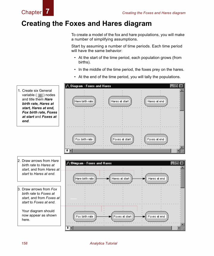
Chapter Creating the Foxes and Hares diagram7
2
3
Creating the Foxes and Hares diagramTo create a model of the fox and hare populations, you will make a number of simplifying assumptions.
Start by assuming a number of time periods. Each time period will have the same behavior:
• At the start of the time period, each population grows (from births).
• In the middle of the time period, the foxes prey on the hares.
• At the end of the time period, you will tally the populations.
1. Create six General variable ( ) nodes and title them Hare birth rate, Hares at start, Hares at end, Fox birth rate, Foxes at start and Foxes at end.
. Draw arrows from Hare birth rate to Hares at start, and from Hares at start to Hares at end.
. Draw arrows from Fox birth rate to Foxes at start, and from Foxes at start to Foxes at end.
Your diagram should now appear as shown here.
158 Analytica Tutorial
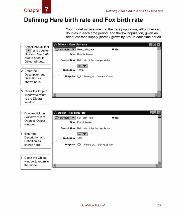
Chapter Defining Hare birth rate and Fox birth rate7
4
5
6
Defining Hare birth rate and Fox birth rateYour model will assume that the hare population, left unchecked, doubles in each time period, and the fox population, given an adequate food supply (hares), grows by 35% in each time period.
1. Select the Edit tool ( ) and double-click on Hare birth rate to open its Object window.
2. Enter the Description and Definition as shown here.
3. Close the Object window to return to the Diagram window.
. Double-click on Fox birth rate to Open its Object window.
. Enter the Description and Definition as shown here.
. Close the Object window to return to the model
Analytica Tutorial 159
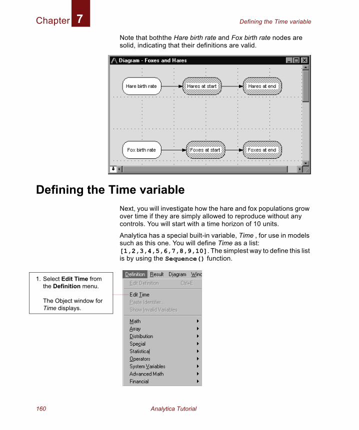
Chapter Defining the Time variable7
Note that boththe Hare birth rate and Fox birth rate nodes are solid, indicating that their definitions are valid.Defining the Time variableNext, you will investigate how the hare and fox populations grow over time if they are simply allowed to reproduce without any controls. You will start with a time horizon of 10 units.
Analytica has a special built-in variable, Time , for use in models such as this one. You will define Time as a list: [1,2,3,4,5,6,7,8,9,10]. The simplest way to define this list is by using the Sequence() function.
1. Select Edit Time from the Definition menu.
The Object window for Time displays.
160 Analytica Tutorial
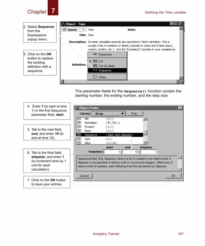
Chapter Defining the Time variable7
2
3
.
The parameter fields for the Sequence() function contain the starting number, the ending number, and the step size.
. Select Sequence from the Expressions popup menu.
. Click on the OK button to replace the existing definition with a sequence.
4. Enter 1 (to start at time 1) in the first Sequence parameter field, start.
5. Tab to the next field, end, and enter 10 (to end at time 10).
6. Tab to the third field, stepsize, and enter 1 (to increment time by 1 unit for each calculation).
7. Click on the OK button to save your entries.
Analytica Tutorial 161
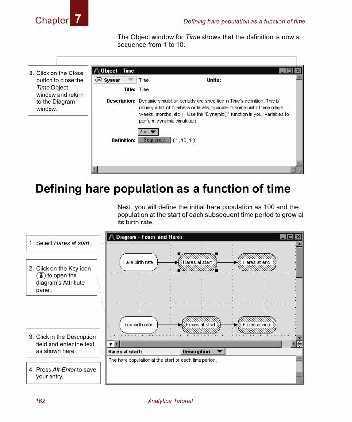
Chapter Defining hare population as a function of time7
1
2
3
4
The Object window for Time shows that the definition is now a sequence from 1 to 10.
Defining hare population as a function of timeNext, you will define the initial hare population as 100 and the population at the start of each subsequent time period to grow at its birth rate.
8. Click on the Close button to close the Time Object window and return to the Diagram window.
. Select Hares at start .
. Click on the Key icon ( ) to open the diagram’s Attribute panel.
. Click in the Description field and enter the text as shown here.
. Press Alt-Enter to save your entry.
162 Analytica Tutorial
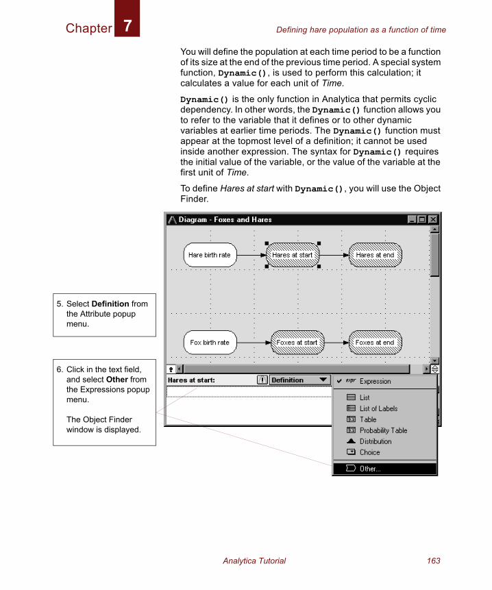
Chapter Defining hare population as a function of time7
5
6
You will define the population at each time period to be a function of its size at the end of the previous time period. A special system function, Dynamic(), is used to perform this calculation; it calculates a value for each unit of Time.
Dynamic() is the only function in Analytica that permits cyclic dependency. In other words, the Dynamic() function allows you to refer to the variable that it defines or to other dynamic variables at earlier time periods. The Dynamic() function must appear at the topmost level of a definition; it cannot be used inside another expression. The syntax for Dynamic() requires the initial value of the variable, or the value of the variable at the first unit of Time.
To define Hares at start with Dynamic(), you will use the Object Finder.
. Select Definition from the Attribute popup menu.
. Click in the text field, and select Other from the Expressions popup menu.
The Object Finder window is displayed.
Analytica Tutorial 163
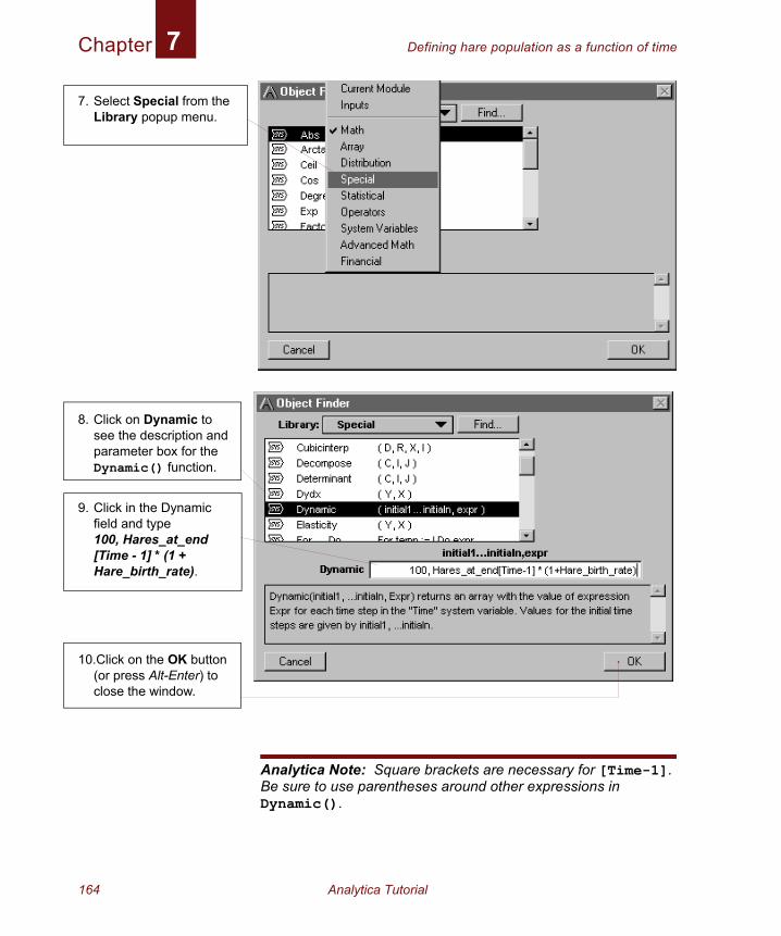
Chapter Defining hare population as a function of time7
Analytica Note: Square brackets are necessary for [Time-1]. Be sure to use parentheses around other expressions in Dynamic().
7. Select Special from the Library popup menu.
8. Click on Dynamic to see the description and parameter box for the Dynamic() function.
9. Click in the Dynamic field and type100, Hares_at_end [Time - 1] * (1 + Hare_birth_rate).
10.Click on the OK button (or press Alt-Enter) to close the window.
164 Analytica Tutorial
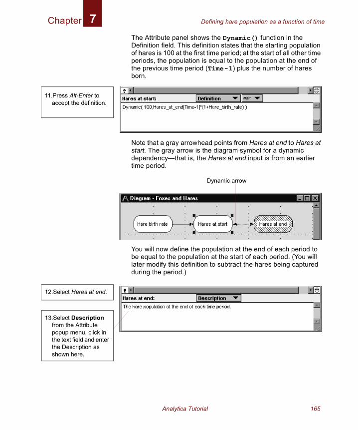
Chapter Defining hare population as a function of time7
The Attribute panel shows the Dynamic() function in the Definition field. This definition states that the starting population of hares is 100 at the first time period; at the start of all other time periods, the population is equal to the population at the end of the previous time period (Time-1) plus the number of hares born.Note that a gray arrowhead points from Hares at end to Hares at start. The gray arrow is the diagram symbol for a dynamic dependency—that is, the Hares at end input is from an earlier time period.
You will now define the population at the end of each period to be equal to the population at the start of each period. (You will later modify this definition to subtract the hares being captured during the period.)
11.Press Alt-Enter to accept the definition.
Dynamic arrow
12.Select Hares at end.
13.Select Description from the Attribute popup menu, click in the text field and enter the Description as shown here.
Analytica Tutorial 165
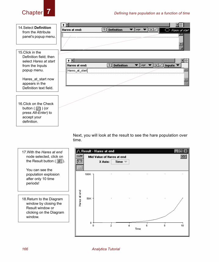
Chapter Defining hare population as a function of time7
1
1
1
Next, you will look at the result to see the hare population over time.
4.Select Definition from the Attribute panel’s popup menu.
5.Click in the Definition field; then select Hares at start from the Inputs popup menu.
Hares_at_start now appears in the Definition text field.
6.Click on the Check button ( ) (or press Alt-Enter) to accept your definition.
17.With the Hares at end node selected, click on the Result button ( ).
You can see the population explosion after only 10 time periods!
18.Return to the Diagram window by closing the Result window or clicking on the Diagram window.
166 Analytica Tutorial
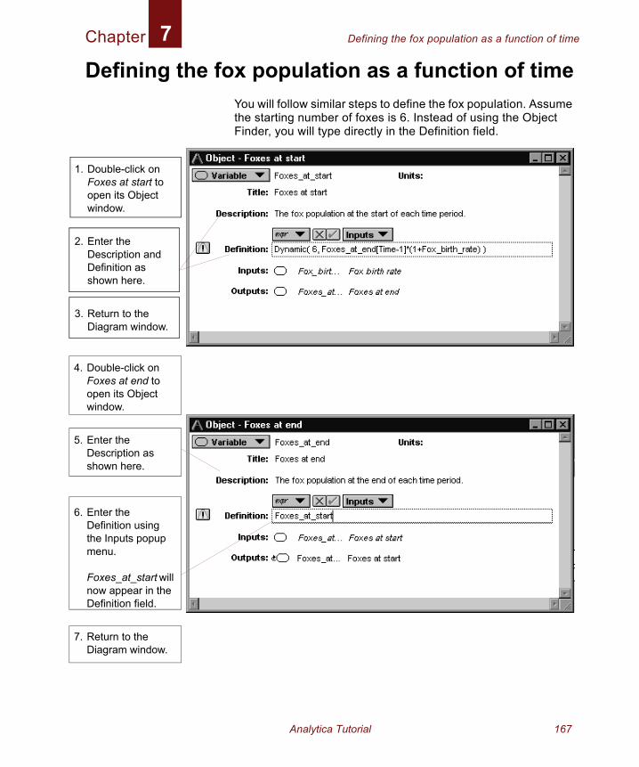
Chapter Defining the fox population as a function of time7
4
5
6
7
Defining the fox population as a function of timeYou will follow similar steps to define the fox population. Assume the starting number of foxes is 6. Instead of using the Object Finder, you will type directly in the Definition field.
1. Double-click on Foxes at start to open its Object window.
2. Enter the Description and Definition as shown here.
3. Return to the Diagram window.
. Double-click on Foxes at end to open its Object window.
. Enter the Description as shown here.
. Enter the Definition using the Inputs popup menu.
Foxes_at_start will now appear in the Definition field.
. Return to the Diagram window.
Analytica Tutorial 167
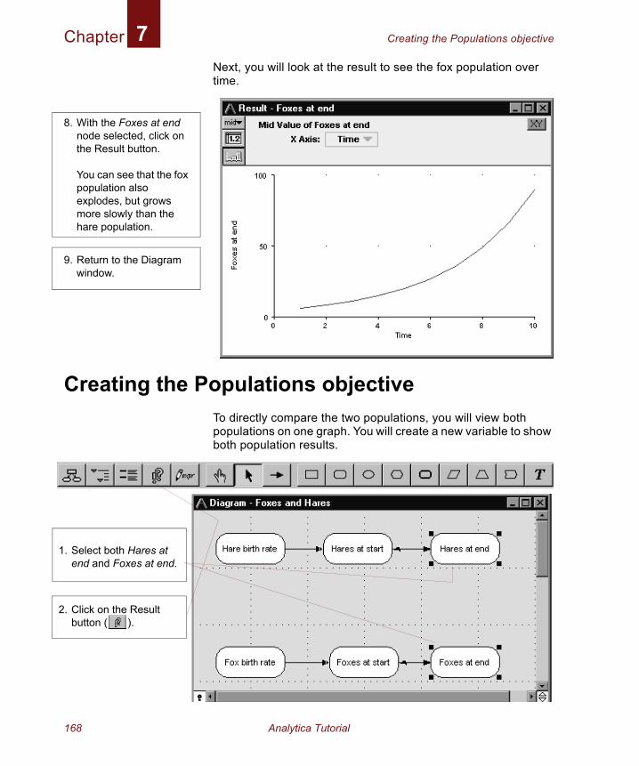
Chapter Creating the Populations objective7
Next, you will look at the result to see the fox population over time.Creating the Populations objective To directly compare the two populations, you will view both populations on one graph. You will create a new variable to show both population results.
8. With the Foxes at end node selected, click on the Result button.
You can see that the fox population also explodes, but grows more slowly than the hare population.
9. Return to the Diagram window.
1. Select both Hares at end and Foxes at end.
2. Click on the Result button ( ).
168 Analytica Tutorial
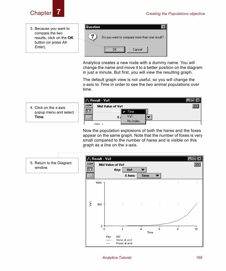
Chapter Creating the Populations objective7
Analytica creates a new node with a dummy name. You will change the name and move it to a better position on the diagram in just a minute. But first, you will view the resulting graph.
The default graph view is not useful, so you will change the x-axis to Time in order to see the two animal populations over time.
Now the population explosions of both the hares and the foxes appear on the same graph. Note that the number of foxes is very small compared to the number of hares and is visible on this graph as a line on the x-axis.
3. Because you want to compare the two results, click on the OK button (or press Alt-Enter).
4. Click on the x-axis popup menu and select Time.
5. Return to the Diagram window.
Analytica Tutorial 169
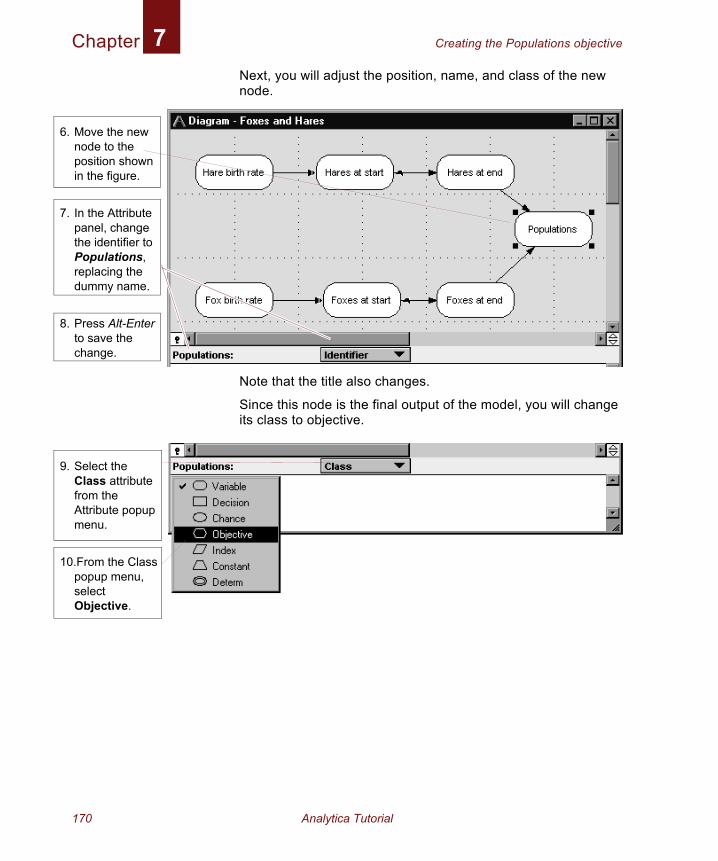
Chapter Creating the Populations objective7
8
Next, you will adjust the position, name, and class of the new node.
Note that the title also changes.
Since this node is the final output of the model, you will change its class to objective.
6. Move the new node to the position shown in the figure.
7. In the Attribute panel, change the identifier to Populations, replacing the dummy name.
. Press Alt-Enter to save the change.
9. Select the Class attribute from the Attribute popup menu.
10.From the Class popup menu, select Objective.
170 Analytica Tutorial
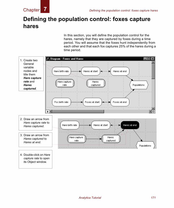
Chapter Defining the population control: foxes capture hares7
1
2
3
4
Defining the population control: foxes capture hares
In this section, you will define the population control for the hares, namely that they are captured by foxes during a time period. You will assume that the foxes hunt independently from each other and that each fox captures 25% of the hares during a time period.
. Create two General variable nodes and title them Hare capture rate and Hares captured.
. Draw an arrow from Hare capture rate to Hares captured.
. Draw an arrow from Hares captured to Hares at end.
. Double-click on Hare capture rate to open its Object window.
Analytica Tutorial 171
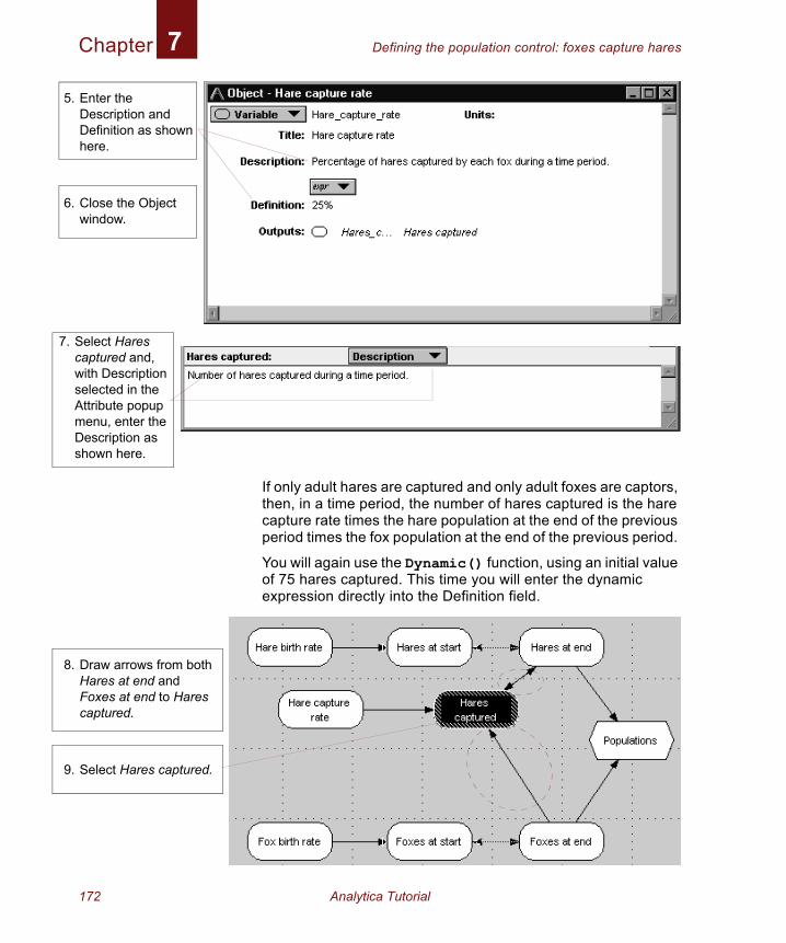
Chapter Defining the population control: foxes capture hares7
5
6
7
8
9
If only adult hares are captured and only adult foxes are captors, then, in a time period, the number of hares captured is the hare capture rate times the hare population at the end of the previous period times the fox population at the end of the previous period.
You will again use the Dynamic() function, using an initial value of 75 hares captured. This time you will enter the dynamic expression directly into the Definition field.
. Enter the Description and Definition as shown here.
. Close the Object window.
. Select Hares captured and, with Description selected in the Attribute popup menu, enter the Description as shown here.
. Draw arrows from both Hares at end and Foxes at end to Hares captured.
. Select Hares captured.
172 Analytica Tutorial
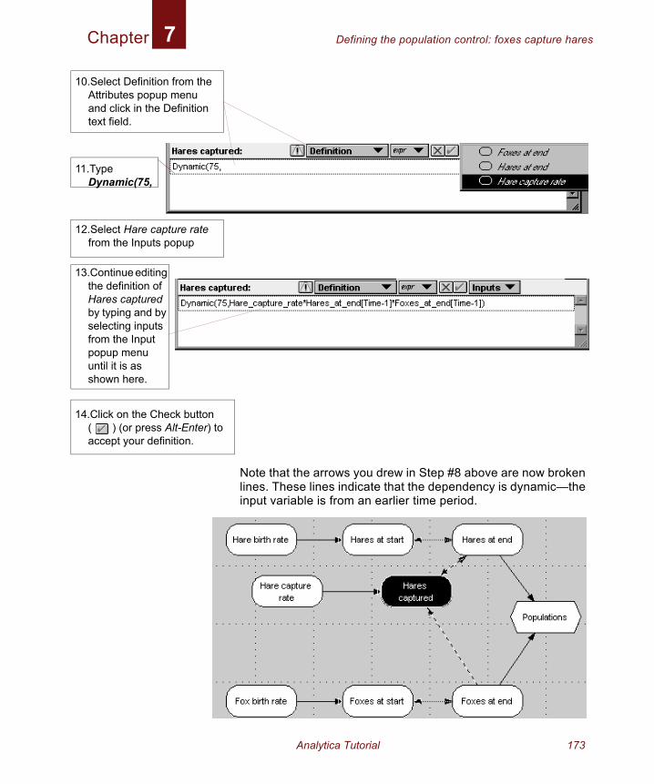
Chapter Defining the population control: foxes capture hares7
1
1
1
1
1
Note that the arrows you drew in Step #8 above are now broken lines. These lines indicate that the dependency is dynamic—the input variable is from an earlier time period.
0.Select Definition from the Attributes popup menu and click in the Definition text field.
1.Type Dynamic(75,
2.Select Hare capture rate from the Inputs popup
3.Continue editing the definition of Hares captured by typing and by selecting inputs from the Input popup menu until it is as shown here.
4.Click on the Check button ( ) (or press Alt-Enter) to accept your definition.
Analytica Tutorial 173
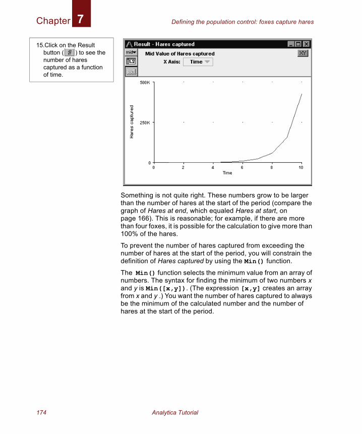
Chapter Defining the population control: foxes capture hares7
Something is not quite right. These numbers grow to be larger than the number of hares at the start of the period (compare the graph of Hares at end, which equaled Hares at start, on page 166). This is reasonable; for example, if there are more than four foxes, it is possible for the calculation to give more than 100% of the hares.
To prevent the number of hares captured from exceeding the number of hares at the start of the period, you will constrain the definition of Hares captured by using the Min() function.
The Min() function selects the minimum value from an array of numbers. The syntax for finding the minimum of two numbers x and y is Min([x,y]). (The expression [x,y] creates an array from x and y .) You want the number of hares captured to always be the minimum of the calculated number and the number of hares at the start of the period.
15.Click on the Result button ( ) to see the number of hares captured as a function of time.
174 Analytica Tutorial
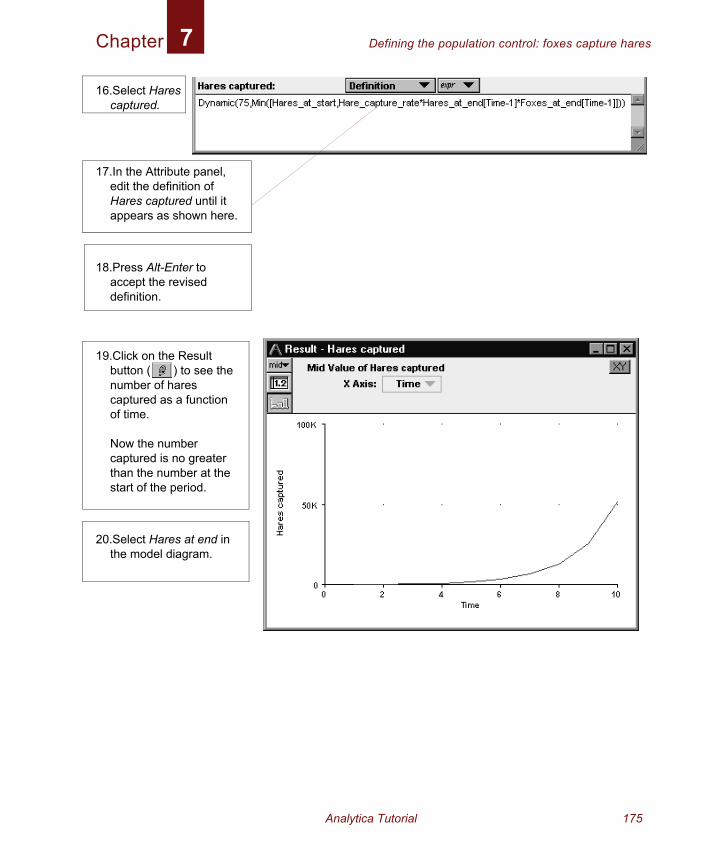
Chapter Defining the population control: foxes capture hares7
16.Select Harescaptured.
17.In the Attribute panel, edit the definition of Hares captured until it appears as shown here.
18.Press Alt-Enter to accept the revised definition.
19.Click on the Result button ( ) to see the number of hares captured as a function of time.
Now the number captured is no greater than the number at the start of the period.
20.Select Hares at end in the model diagram.
Analytica Tutorial 175
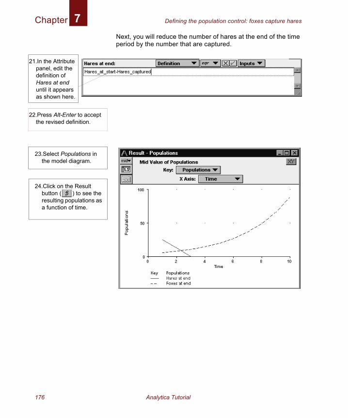
Chapter Defining the population control: foxes capture hares7
2
Next, you will reduce the number of hares at the end of the time period by the number that are captured.
21.In the Attribute panel, edit the definition of Hares at end until it appearsas shown here.
2.Press Alt-Enter to accept the revised definition.
23.Select Populations in the model diagram.
24.Click on the Result button ( ) to see the resulting populations as a function of time.
176 Analytica Tutorial
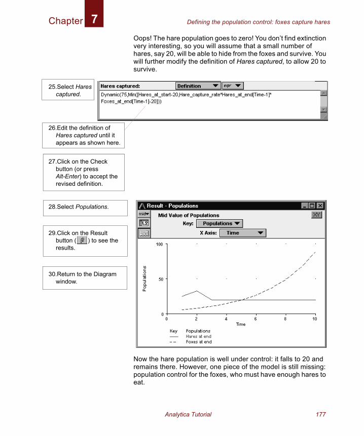
Chapter Defining the population control: foxes capture hares7
Oops! The hare population goes to zero! You don’t find extinction very interesting, so you will assume that a small number of hares, say 20, will be able to hide from the foxes and survive. You will further modify the definition of Hares captured, to allow 20 to survive.Now the hare population is well under control: it falls to 20 and remains there. However, one piece of the model is still missing: population control for the foxes, who must have enough hares to eat.
25.Select Hares captured.
26.Edit the definition of Hares captured until it appears as shown here.
27.Click on the Check button (or press Alt-Enter) to accept the revised definition.
28.Select Populations.
29.Click on the Result button ( ) to see the results.
30.Return to the Diagram window.
Analytica Tutorial 177
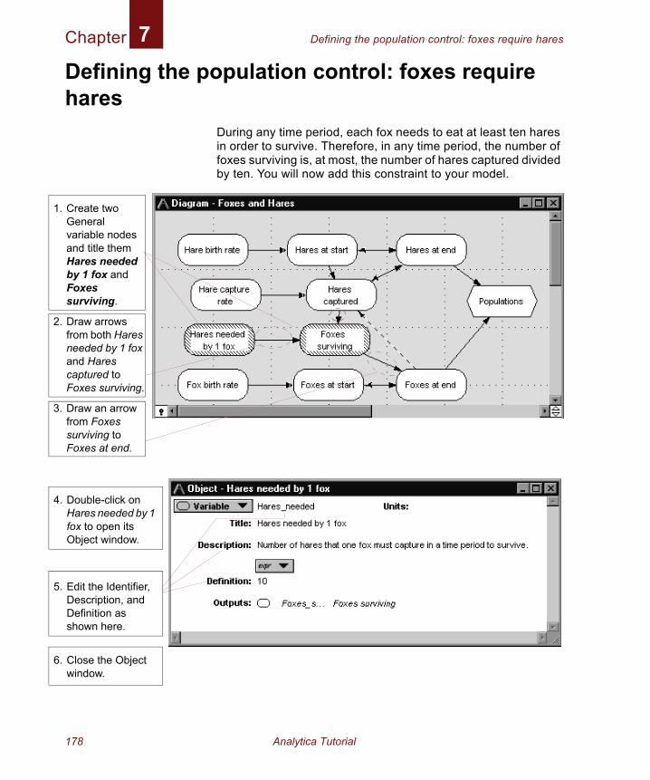
Chapter Defining the population control: foxes require hares7
1
2
3
4
5
6
Defining the population control: foxes require hares
During any time period, each fox needs to eat at least ten hares in order to survive. Therefore, in any time period, the number of foxes surviving is, at most, the number of hares captured divided by ten. You will now add this constraint to your model.
. Create two General variable nodes and title them Hares needed by 1 fox and Foxes surviving.
. Draw arrows from both Hares needed by 1 fox and Hares captured to Foxes surviving.
. Draw an arrow from Foxes surviving to Foxes at end.
. Double-click on Hares needed by 1 fox to open its Object window.
. Edit the Identifier, Description, and Definition as shown here.
. Close the Object window.
178 Analytica Tutorial
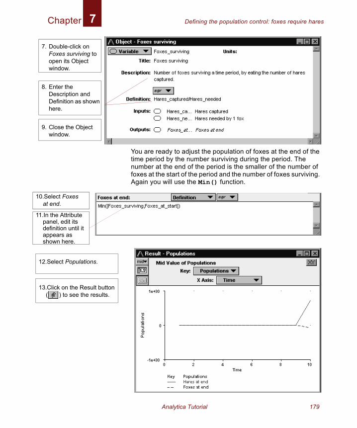
Chapter Defining the population control: foxes require hares7
10
11
1
1
You are ready to adjust the population of foxes at the end of the time period by the number surviving during the period. The number at the end of the period is the smaller of the number of foxes at the start of the period and the number of foxes surviving. Again you will use the Min() function.
7. Double-click on Foxes surviving to open its Object window.
8. Enter the Description and Definition as shown here.
9. Close the Object window.
.Select Foxes at end.
.In the Attribute panel, edit its definition until it appears as shown here.
2.Select Populations.
3.Click on the Result button ( ) to see the results.
Analytica Tutorial 179
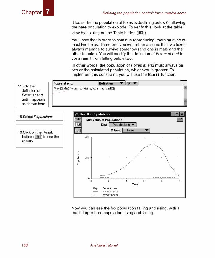
Chapter Defining the population control: foxes require hares7
1
It looks like the population of foxes is declining below 0, allowing the hare population to explode! To verify this, look at the table view by clicking on the Table button ( ).
You know that in order to continue reproducing, there must be at least two foxes. Therefore, you will further assume that two foxes always manage to survive somehow (and one is male and the other female!). You will modify the definition of Foxes at end to constrain it from falling below two.
In other words, the population of Foxes at end must always be two or the calculated population, whichever is greater. To implement this constraint, you will use the Max() function.
Now you can see the fox population falling and rising, with a much larger hare population rising and falling.
4.Edit the definition of Foxes at end until it appears as shown here.
15.Select Populations.
16.Click on the Result button ( ) to see the results.
180 Analytica Tutorial
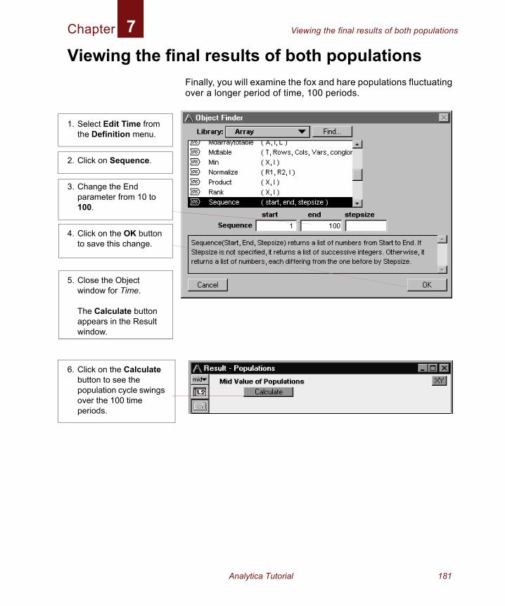
Chapter Viewing the final results of both populations7
Viewing the final results of both populationsFinally, you will examine the fox and hare populations fluctuating over a longer period of time, 100 periods.
1. Select Edit Time from the Definition menu.
2. Click on Sequence.
3. Change the End parameter from 10 to 100.
4. Click on the OK button to save this change.
5. Close the Object window for Time.
The Calculate button appears in the Result window.
6. Click on the Calculate button to see the population cycle swings over the 100 time periods.
Analytica Tutorial 181
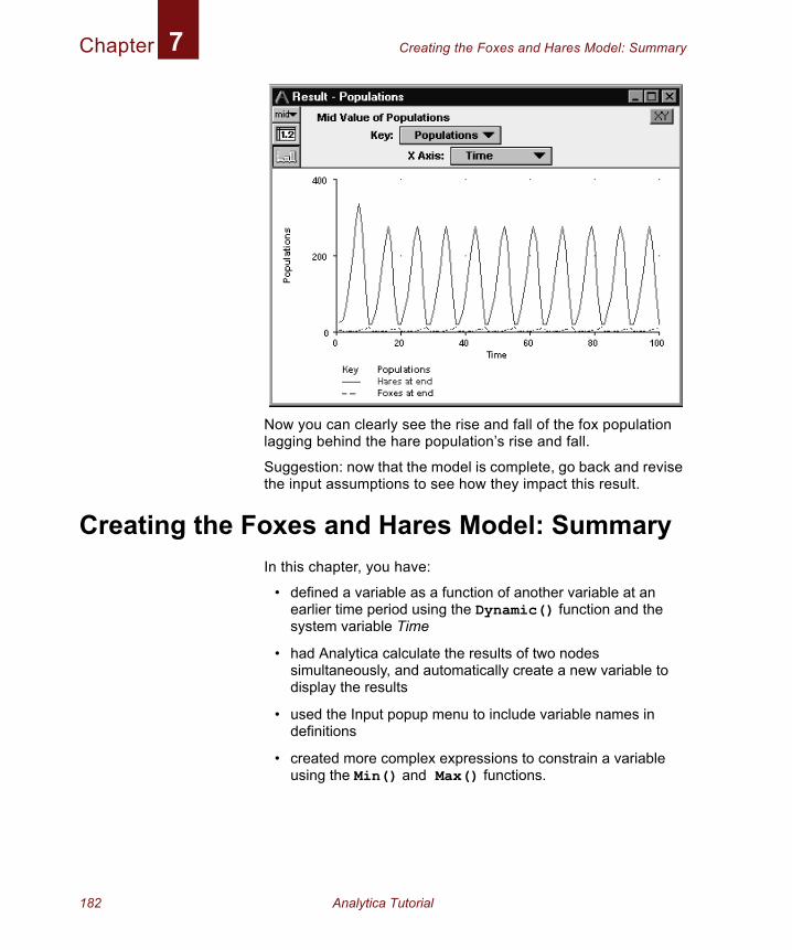
Chapter Creating the Foxes and Hares Model: Summary7
Now you can clearly see the rise and fall of the fox population lagging behind the hare population’s rise and fall.
Suggestion: now that the model is complete, go back and revise the input assumptions to see how they impact this result.
Creating the Foxes and Hares Model: SummaryIn this chapter, you have:
• defined a variable as a function of another variable at an earlier time period using the Dynamic() function and the system variable Time
• had Analytica calculate the results of two nodes simultaneously, and automatically create a new variable to display the results
• used the Input popup menu to include variable names in definitions
• created more complex expressions to constrain a variable using the Min() and Max() functions.
182 Analytica Tutorial

Chapter 8
On Your Own

In this Chapter
This chapter describes the example models provided with Analytica.
Chapter 8: On Your OwnCongratulations on completing the Analytica Tutorial. You are now ready to begin creating your own models.
For more detailed information on Analytica, see the Analytica User Guide. It is a reference on all aspects of Analytica, including descriptions of all available functions.
Within the Analytica folder are folders titled Example Models and Libraries, which contains a variety of Analytica models, including all the examples illustrated in the Analytica User Guide, as libraries that are useful to include when building your own models. Many of the example models were created by users just like you. These models contain a wealth of ideas on using Analytica for practical applications. You should investigate these examples to see some of the different ways in which models can be constructed.
If you create models that you feel would be helpful or interesting to others, please send them to us for inclusion in a future Example Models folder; see the Analytica User Guide, Appendix H, “How to Contact Us”, or see the end of this chapter.
The Example Models folder is subdivided into these folders:
• Business Examples
• Decision Analysis
• Dynamic Models
• Function Examples
• Risk Analysis
• User Guide Examples
Business ExamplesBond Model
This model takes typical bond purchase inputs (purchase price, par value, interest rate, and life to maturity) and calculates bond cash flows, current yield and yield to maturity.
Analytica Tutorial 185
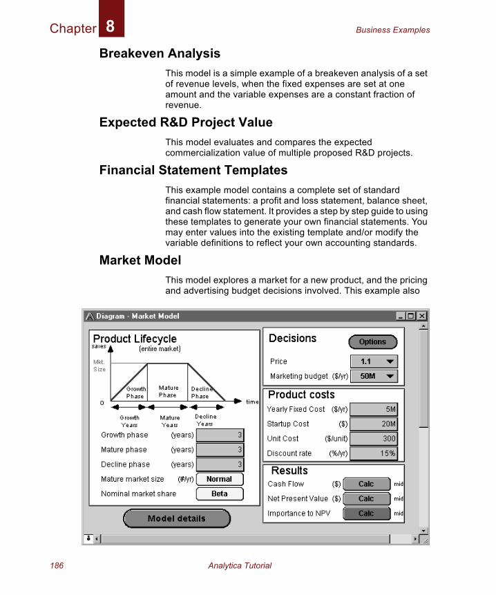
Chapter Business Examples8
Breakeven AnalysisThis model is a simple example of a breakeven analysis of a set of revenue levels, when the fixed expenses are set at one amount and the variable expenses are a constant fraction of revenue.
Expected R&D Project ValueThis model evaluates and compares the expected commercialization value of multiple proposed R&D projects.
Financial Statement TemplatesThis example model contains a complete set of standard financial statements: a profit and loss statement, balance sheet, and cash flow statement. It provides a step by step guide to using these templates to generate your own financial statements. You may enter values into the existing template and/or modify the variable definitions to reflect your own accounting standards.
Market ModelThis model explores a market for a new product, and the pricing and advertising budget decisions involved. This example also
186 Analytica Tutorial
Chapter Business Examples8
shows the use of “forms” for receiving input and presenting output for users of the model.Plan_Schedule_ControlThis model takes input data for activity paths required to complete a project, and calculates various outputs describing the critical path, timing and costs for project completion.
Sales EffectivenessThis model evaluates the effects of unit price on salesmen headcount and production capacity. The model contains an example of taking user estimates of uncertainty in a standard high-medium-low form, and transforming those inputs into a continuous distribution for propagation through the model.
Derived from Principles of Systems by Jay W. Forrester, 1968, ISBN 0-915299-87-9.
Subscriber PricingThe purpose of this model is to determine the amount of revenue needed on a monthly basis from each subscriber of a service to just meet the weighted average cost of capital of the firm from the service release date to the end of the Study Horizon. In other words, it calculates the monthly unit revenue rate required from each subscriber of a service to give a return on investment at the end of the Study Horizon that is equal to the weighted average cost of capital of the firm.
Analytica Tutorial 187
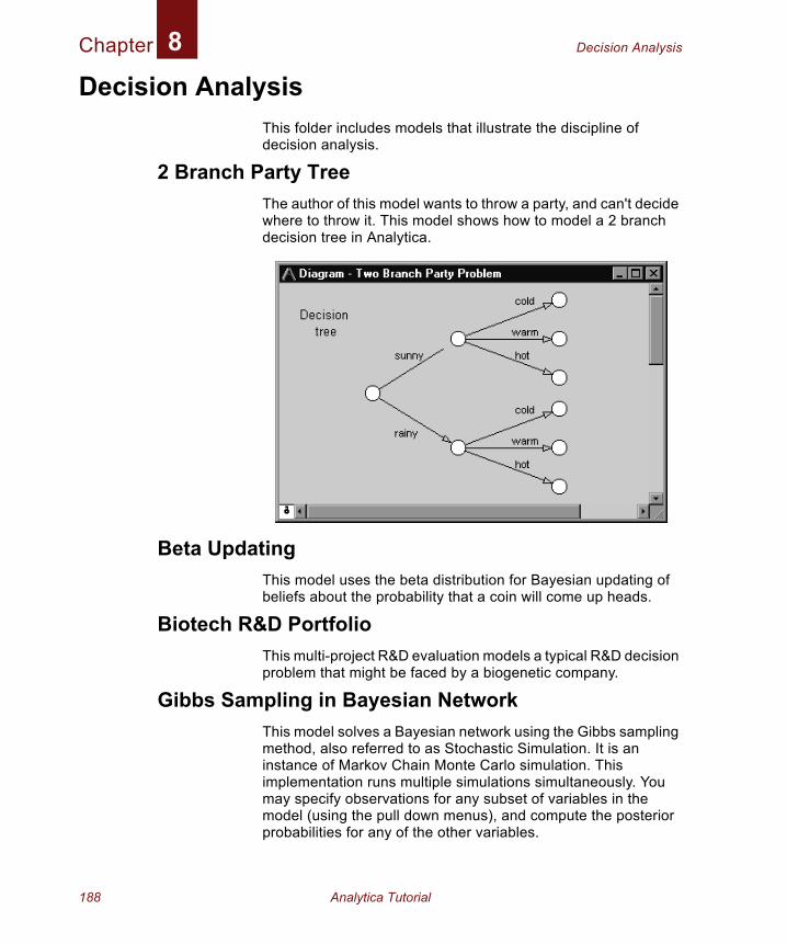
Chapter Decision Analysis8
Decision AnalysisThis folder includes models that illustrate the discipline of decision analysis.
2 Branch Party TreeThe author of this model wants to throw a party, and can't decide where to throw it. This model shows how to model a 2 branch decision tree in Analytica.
Beta UpdatingThis model uses the beta distribution for Bayesian updating of beliefs about the probability that a coin will come up heads.
Biotech R&D PortfolioThis multi-project R&D evaluation models a typical R&D decision problem that might be faced by a biogenetic company.
Gibbs Sampling in Bayesian NetworkThis model solves a Bayesian network using the Gibbs sampling method, also referred to as Stochastic Simulation. It is an instance of Markov Chain Monte Carlo simulation. This implementation runs multiple simulations simultaneously. You may specify observations for any subset of variables in the model (using the pull down menus), and compute the posterior probabilities for any of the other variables.
188 Analytica Tutorial
Chapter Decision Analysis8
For more on this technique, see S. L. Lauritzen & D. J. Spiegelhalter, “Local Computations with Probabilities on Graphical Structures and Their Application to Expert Systems”, Journal Royal Statistical Society Series B50:2, 1984, p. 157-224.LEV R&D StrategyThis example models R&D decision analysis for investment strategy among several choices of powerplants for a Low Emissions Vehicle (LEV).
Newton-Raphson MethodThis model implements the Newton-Raphson (or simply Newton's) method, one of the most powerful and well-known numerical methods for finding the root of f(x)=0.
Nonsymmetric TreeThis model is an example of what, using decision tree terminology, would be an asymmetric decision tree in Analytica.
Party With ForecastThis model presents a problem facing a party host. In the face of uncertain weather, what is the best location to hold a party? The value the host assigns to the party is a function of both the location chosen and the weather outcome.
This model augments the basic party model in order to show the value of imperfect information—in this case, a weather forecast—using Bayesian updating.
Supply and DemandThis model calculates the required supply level to maximize profit when the profit function is asymmetric around the average demand value.
Tornado DiagramsA Tornado diagram is a common tool used to depict the sensitivity of a result to changes in selected variables. The fundamental analysis behind a tornado diagram consists of varying only one input variable at a time, keeping all other variables at their nominal values. Typically, a Low and a High value are selected for each input, and the output variable is computed while only one variable varies at a time. This example model shows two methods for selecting high and low values: 1. by varying all inputs by the same relative amount, e.g., low=90%
Analytica Tutorial 189

Chapter Decision Analysis8
of nominal, high=110% of nominal, or 2. by varying all inputs between two given fractiles. This only makes sense if your inputs are uncertain variables. Example: Low=10% fractile, High=90% fractile, nominal=50% fractile.Note that Analytica's built-in graphing tool can produce only vertical bar graphs, allowing only rotated tornado diagrams to be created. The conventional (non-rotated) tornado diagram can be obtained using Excel Graph from within Analytica. An example of plotting with both Analytica and Excel are given in the example.
190 Analytica Tutorial
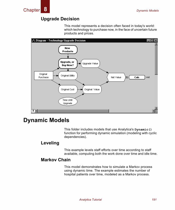
Chapter Dynamic Models8
Upgrade DecisionThis model represents a decision often faced in today's world: which technology to purchase now, in the face of uncertain future products and prices.
Dynamic ModelsThis folder includes models that use Analytica's Dynamic() function for performing dynamic simulation (modeling with cyclic dependencies).
LevelingThis example levels staff efforts over time according to staff available, computing both the work done over time and idle time.
Markov ChainThis model demonstrates how to simulate a Markov process using dynamic time. The example estimates the number of hospital patients over time, modeled as a Markov process.
Analytica Tutorial 191
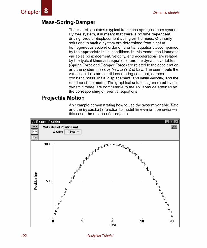
Chapter Dynamic Models8
Mass-Spring-DamperThis model simulates a typical free mass-spring-damper system. By free system, it is meant that there is no time dependent driving force or displacement acting on the mass. Ordinarily solutions to such a system are determined from a set of homogeneous second order differential equations accompanied by the appropriate initial conditions. In this model, the kinematic variables (displacement, velocity, and acceleration) are related by the typical kinematic equations, and the dynamic variables (Spring Force and Damper Force) are related to the acceleration and the system mass by Newton's 2nd Law. The user inputs the various initial state conditions (spring constant, damper constant, mass, initial displacement, and initial velocity) and the run time of the model. The graphical solutions generated by this dynamic model are comparable to the solutions determined by the corresponding differential equations.
Projectile MotionAn example demonstrating how to use the system variable Time and the Dynamic() function to model time-variant behavior—in this case, the motion of a projectile.
192 Analytica Tutorial
Chapter Engineering Examples8
Unequal time stepsThis model gives an example of a dynamic variable that calculates growth over time, where Time is defined with unequal time steps. It is an example of exponential and/or linear growth or decay—that is, a dynamic variable whose values in one time period are exponentially or linearly dependent on the values in the previous time period.
Engineering ExamplesAdaptive Filter
This model curve-fits noisy time sequence data using an adaptive filter.
Antenna GainThis model calculates the expected gain of an antenna looking at two different satellites.
Failure AnalysisThis model provides a system simulation demonstrating a failure analysis with both parallel (bulbs) and series (bulbs and switch) components. The model shows use of a Determtable instead of nested if...then statements to assess the state of the system. Both the switch and the bulbs use an exponential function to assess the probability of failure.
Function ExamplesThis folder contains examples illustrating a variety of Analytica’s functions and modeling techniques.
AutocorrelationThis model calculates the autocorrelation coefficients of noisy time sequence data.
Choice and DetermtableThis model shows that when Choice nodes are indexed by 'self', you can use Determtables to propagate the selected choice. This is cleaner than some other methods of using Choice outputs.
Analytica Tutorial 193
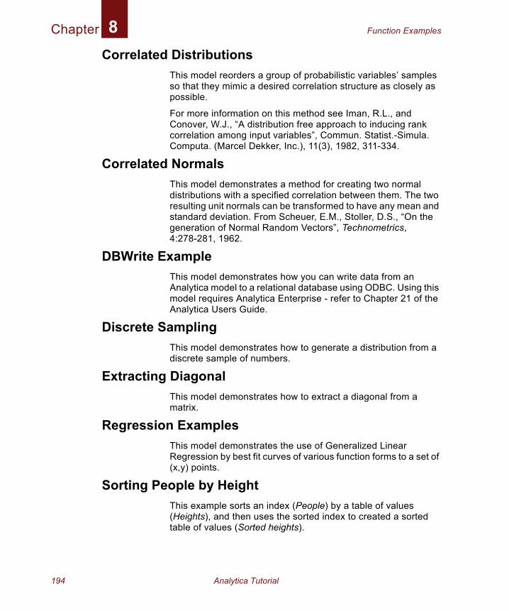
Chapter Function Examples8
Correlated DistributionsThis model reorders a group of probabilistic variables’ samples so that they mimic a desired correlation structure as closely as possible.
For more information on this method see Iman, R.L., and Conover, W.J., “A distribution free approach to inducing rank correlation among input variables”, Commun. Statist.-Simula. Computa. (Marcel Dekker, Inc.), 11(3), 1982, 311-334.
Correlated NormalsThis model demonstrates a method for creating two normal distributions with a specified correlation between them. The two resulting unit normals can be transformed to have any mean and standard deviation. From Scheuer, E.M., Stoller, D.S., “On the generation of Normal Random Vectors”, Technometrics, 4:278-281, 1962.
DBWrite ExampleThis model demonstrates how you can write data from an Analytica model to a relational database using ODBC. Using this model requires Analytica Enterprise - refer to Chapter 21 of the Analytica Users Guide.
Discrete SamplingThis model demonstrates how to generate a distribution from a discrete sample of numbers.
Extracting DiagonalThis model demonstrates how to extract a diagonal from a matrix.
Regression ExamplesThis model demonstrates the use of Generalized Linear Regression by best fit curves of various function forms to a set of (x,y) points.
Sorting People by HeightThis example sorts an index (People) by a table of values (Heights), and then uses the sorted index to created a sorted table of values (Sorted heights).
194 Analytica Tutorial
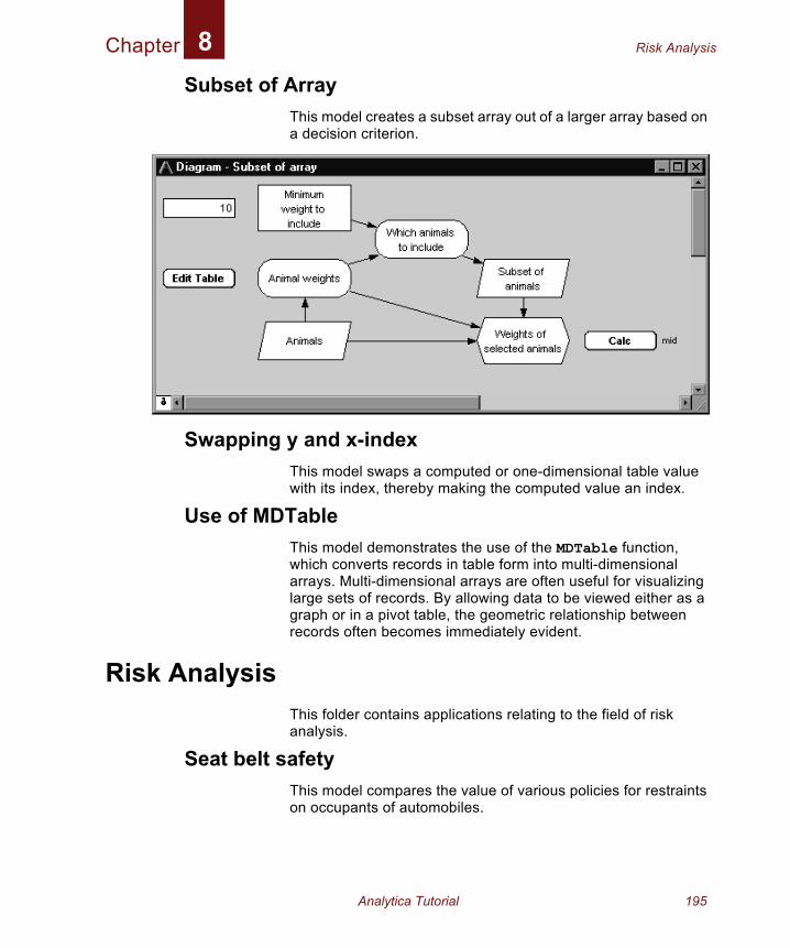
Chapter Risk Analysis8
Subset of ArrayThis model creates a subset array out of a larger array based on a decision criterion.
Swapping y and x-indexThis model swaps a computed or one-dimensional table value with its index, thereby making the computed value an index.
Use of MDTableThis model demonstrates the use of the MDTable function, which converts records in table form into multi-dimensional arrays. Multi-dimensional arrays are often useful for visualizing large sets of records. By allowing data to be viewed either as a graph or in a pivot table, the geometric relationship between records often becomes immediately evident.
Risk AnalysisThis folder contains applications relating to the field of risk analysis.
Seat belt safetyThis model compares the value of various policies for restraints on occupants of automobiles.
Analytica Tutorial 195
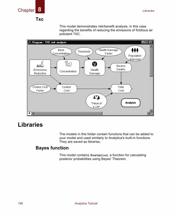
Chapter Libraries8
TxcThis model demonstrates risk/benefit analysis, in this case regarding the benefits of reducing the emissions of fictitious air pollutant TXC.
LibrariesThe models in this folder contain functions that can be added to your model and used similarly to Analytica's built-in functions. They are saved as libraries.
Bayes functionThis model contains Posterior, a function for calculating posterior probabilities using Bayes' Theorem.
196 Analytica Tutorial
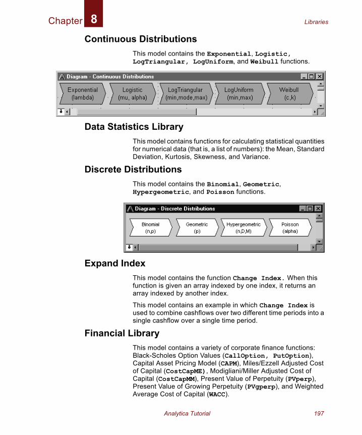
Chapter Libraries8
Continuous DistributionsThis model contains the Exponential, Logistic, LogTriangular, LogUniform, and Weibull functions.
Data Statistics LibraryThis model contains functions for calculating statistical quantities for numerical data (that is, a list of numbers): the Mean, Standard Deviation, Kurtosis, Skewness, and Variance.
Discrete DistributionsThis model contains the Binomial, Geometric, Hypergeometric, and Poisson functions.
Expand IndexThis model contains the function Change Index. When this function is given an array indexed by one index, it returns an array indexed by another index.
This model contains an example in which Change Index is used to combine cashflows over two different time periods into a single cashflow over a single time period.
Financial LibraryThis model contains a variety of corporate finance functions: Black-Scholes Option Values (CallOption, PutOption), Capital Asset Pricing Model (CAPM), Miles/Ezzell Adjusted Cost of Capital (CostCapME), Modigliani/Miller Adjusted Cost of Capital (CostCapMM), Present Value of Perpetuity (PVperp), Present Value of Growing Perpetuity (PVgperp), and Weighted Average Cost of Capital (WACC).
Analytica Tutorial 197
Chapter User Guide Examples8
ODBC-LibraryThis library provides additional functionality (ValList, InsertRecSql, WriteTableSql) for using ODBC access to databases. Note that using ODBC requires Analytica Enterprise - refer to Chapter 21 of the Analytica Users Guide.
User Guide ExamplesThis folder contains the examples that are given in the Analytica User Guide.
Analyzing Unc & SensThe examples in this model demonstrate Analytica's tools for analyzing the uncertainty of variables, relationships between uncertain variables, and sensitivity of outputs to changes in inputs. These include statistical functions and sensitivity analysis functions.
This model is used in User Guide Chapter 16, “Analyzing Uncertainty and Sensitivity”.
Array ExamplesThe examples in this model demonstrate the basics of working with multidimensional arrays.
This model is used in User Guide Chapter 11, “Basic Modeling with Arrays (Tables)”.
Array Function ExamplesThe examples in this model demonstrate many more of Analytica's built-in array functions.
This model is used in User Guide Chapter 12, “Array Function Reference”.
Continuous DistributionsA continuous distribution is one that is defined for a continuous variable—that is, for a real-valued variable. The examples in this model demonstrate Analytica's built-in functions that create or modify continuous distributions.
This model is used in User Guide Chapter 14, “Using Continuous Probability Distributions”.
198 Analytica Tutorial
Chapter User Guide Examples8
Discrete DistributionsA discrete distribution is a probability distribution for a variable that can result only in certain, discrete outcomes. The examples in this model demonstrate Analytica's built-in functions that create or evaluate discrete distributions.
This model is used in User Guide Chapter 15, “Using Discrete Probability”.
Dynamic & Dependencies
Dynamic & Uncertainty
Dynamic Example 1
Dynamic Example 2These are dynamic models. A dynamic model is a model with one or more dynamic variables—that is, variables that can change over time. These models illustrate various uses of the Dynamic function.
These models are used in User Guide Chapter 17, “Modeling Changes over Time”.
Expression ExamplesThe examples in this model demonstrate the building blocks for creating and editing variable definitions—expressions, standard operators, and mathematical functions.
This model is used in User Guide Chapter 10, “Using Expressions”.
Input and Output NodesThis model is used in User Guide Chapter 9, “Creating Models to be Used by Others”.
Analytica Tutorial 199
Chapter On Your Own Summary8
SummaryIf you have created a model that other Analytica users would benefit from, please send it to us for possible inclusion in future versions of the Example Models folder. Send your well-constructed, thoroughly documented models to:
Also, if you experience any problems with the example models, or if you feel that they need to be changed in some way, please contact us at the above email address.
200 Analytica Tutorial

Glossary

In this Glossary
A compilation of terms specific to Analytica as well as statistical terms used in this manual.
Glossary
ArrayA collection of values that can be viewed as one or more tables. An array has one or more dimensions; each dimension is identified by an index.Arrow, influence arrowInfluence arrows (or arrows) from one variable node to another indicate that the origin node affects (influences) the destination node. If the nodes depict variables, the origin variable is an input to the destination variable, and the destination variable is an output of the origin variable.
Arrow toolThe tool for drawing arrows between nodes.
AttributeA property of an object, such as its title, description, definition, value, or inputs.
Attribute panelAn auxiliary window pane that can open below an influence diagram. Use it to rapidly examine one attribute at a time of any variable, function, or module.
Browse toolA tool for examining the structure and assumptions of a model, with limited ability to make changes to the model.
Chance variableAn uncertain variable that cannot be directly controlled by the decision maker. It is usually defined by a probability distribution. A Chance variable is represented by an oval node.
ClassAnalytica objects are organized into the following classes: Module, Attribute, Function, and Decision, Chance, Objective, Index, and General variables.
Analytica Tutorial 203
Glossary
Cumulative probability distributionA graphical representation of a probability distribution. It plots the cumulative probability that the actual value of the uncertain variable X will be less than or equal to each possible value of X. The cumulative probability distribution is a display option in the Uncertainty View popup menu on a Result window.Decision variableA variable that the decision maker can control directly. A Decision variable is represented by a rectangular node.
DefinitionA specification for computing a variable’s value. It can be a number, a mathematical expression, a list of values, a table, or a probability distribution.
DescriptionText explaining what the object represents in the system being modeled. It is limited in length to 32,000 characters.
Deterministic tableA function that gives the value of a variable conditional on the values of its input variables, where the inputs are all discrete variables.
Deterministic valueSee mid value.
DomainThe possible outcomes for a variable defined as a probability table.
Edit TableA definition that is an array (table) is also called an Edit Table because it can be edited.
204 Analytica Tutorial
Glossary
Edit toolA tool for creating or changing a model. Use it to move, resize and edit nodes, and expose the Arrow tool and Node palette.
ExpressionA formula that can contain any combination of numbers, variables, functions, distributions, and operators, such as 0.5, a-b, or Min(x), combined according to the Analytica language syntax.
Expression typeExpression types include expression, list (of expressions or numbers), list of labels (text strings), table, probability table, and distribution. (Any definition, regardless of expression type, can be viewed as an expression.) You select an expression type using the Expression popup menu, which appears above the Definition field.
General variableAny type of variable; useful when the variable type is unknown. The General variable typically represents a deterministic or functional dependency.
GraphFormat for displaying a multidimensional result. To view a result as a graph, click on the Graph button. See also table.
IdentifierA short name for an object. A variable’s identifier is used to refer to the variable in mathematical expressions in definitions of other variables. An identifier must start with a letter, have no more than 20 characters, and contain only letters, numbers, and ‘_’ (underscore, used instead of a space). Compare to title.
Importance analysisShows the effect the uncertainty of one or more input variables has on the uncertainty of an output variable. Importance is defined as the rank-order correlation between the sample of output values and the sample for each uncertain input. This is a
Analytica Tutorial 205
Glossary
robust measure of the uncertain contribution because it is insensitive to extreme values and skewed distributions.IndexIdentifies a dimension of an array (table). An index is usually a variable defined as a list, list of labels, or sequence.
IndexesPlural of index, indicates a set of index variables that define the dimensions of a table (in an Edit Table or value).
Index variableA class of variable, defined as a list, list of labels, or sequence, that is used to identify the dimensions of a table, for example, in an Edit Table. An Index variable is represented by a parallelogram node.
Influence arrowSee Arrow.
Influence diagramA graphical representation of a model, consisting of nodes (variables) and arrows (relationships between variables).
InputAn input of a variable X is a variable that has an arrow drawn to X, or appears in the definition of X. See also output.
Input arrowheadShows that a node has one or more inputs from outside its module. It is located on the left side of a node. Press the arrowhead for a popup menu of the input variables.
ListA type of expression, consisting of an ordered set of numbers or expressions, available in the Expression popup menu. A list is often used to define Index and Decision variables.
206 Analytica Tutorial
Glossary
List of labelsA type of expression, consisting of an ordered set of text labels, available in the Expression popup menu. A list of labels is often used to define Index and Decision variables.MeanThe average or expected value.
Mid, Mid valueA calculation of the variable's value assuming all uncertain inputs are fixed at their median values.
ModelA module, or a hierarchy of modules; the main, or root, module at the top of the module hierarchy. Between sessions, a model is stored in a Analytica document file.
ModuleA collection of related objects, including variables, functions, and other modules, organized as a separate influence diagram. A module is represented by a rounded rectangular node with a thick outline.
NodeA box (rectangular, oval, or any other shape) that represents a variable in an influence diagram. Different node shapes are used to represent different types of variables.
Normal distributionThe bell-shaped curve, or Gaussian distribution.
Object FinderA dialog box used to browse and edit the functions and variables available in a model.
Object windowList of the attributes for an object (variable, function, or module), including its class, identifier, title, and description.
Analytica Tutorial 207
Glossary
Objective variableA variable that evaluates the overall value or desirability of possible outcomes. The objective can be measured as cost, value, or utility. A purpose of most models is to find the decision or decisions that optimize the objective—for example, minimizing cost or maximizing expected utility. Most decision models contain a single objective node, although the objective can be composed of several subobjectives. An Objective variable is represented by a hexagonal node.
OutputAn output of a variable X is a variable that has an arrow drawn from X, or whose definition refers to X. See also input.
Output arrowheadShows that a node has one or more outputs outside its module. It is located on the right side of the node. Press the arrowhead for a popup menu of the output variables.
Parametric analysisA type of sensitivity analysis in which you specify a set of alternative values for one or more inputs, and examine the effect on selected model output variables. See also sensitivity analysis.
Probabilistic variableA variable that is uncertain and is defined with a probability distribution.
Probability bandsThe bands that capture a certain portion of the total probability for a variable. For example, the 5% and 95% probability bands contain 90% of the total probability, while the 50% probability band corresponds to the median value. By default, the 5%, 25%, 50%, 75%, and 95% probability bands are shown. These bands are also referred to as confidence intervals or fractiles. Probability bands are a display option in the Uncertainty View popup menu on a Result window.
208 Analytica Tutorial
Glossary
Probability density functionA graphical representation of a probability distribution that plots the probability density against the value of the variable (also referred to as PDF). The probability density at each value of X is the relative probability that X will be at or near that value. The probability density function can be displayed for continuous, but not discrete, variables. It is a display option in the Uncertainty View popup menu on a Result window.Probability distributionDescribes the relative likelihood of a variable having different possible values.
Probability tableA table for defining a Chance variable with a set of outcomes and a discrete probability distribution (numerical probability for each outcome). If the variable depends on (that is, is conditioned by) other discrete variables, each of these conditioning variables gives an additional dimension to the table, so you can specify the probability distribution conditional on the value of each conditioning variable.
SelfA keyword referring to the index of a table that is indexed by itself. Self refers to the alternative values of the variable defined by the table.
Sensitivity analysisA group of methods to identify and compare the effects of various input variables to a model on a selected output. Example methods of sensitivity analysis are importance analysis and parametric analysis.
Standard deviationReflects the amount of spread or dispersion in an uncertainty distribution. It is the square root of the variance.
TableA two-dimensional view of an array-valued definition or result. The array can have more than two dimensions, but only two can
Analytica Tutorial 209

Glossary
be seen at one time. A table is a type of expression available in the Expression popup menu. A definition that is a table is also called an Edit Table. In the Result window, click on the Table button to select the table view of an array-valued result. See also graph.TitleThe full name of an Analytica object, briefly describing what the object represents. A variable's, function's, or module's title is displayed in its node, in window titles, and in object lists. It is limited to 255 characters in length. It can contain any characters, including spaces and punctuation. Compare to identifier.
Uniform distributionA distribution representing an equal chance of occurrence for any value between the lower and upper values.
Uncertainty View optionsAn uncertain result can be displayed as a Mid value, Mean, Statistics, Probability Bands, Probability Density, Cumulative Probability, or Sample. Select the option to display with the popup menu in the top left corner of the Result window or in the Result menu.
UnitsIndicate the units of measurement for a variable. Units are used to annotate tables and graphs, but are not used in evaluating a variable.
ValueA variable’s value attribute is its mid value, computed by assuming that all uncertain inputs are fixed at their median values. It can be a scalar (single) number, a table of numbers, or a probability distribution.
VariableAn object that has a value, which may be a text string, a number, or a table. Classes of variable include Decision, Chance, and Objective.
210 Analytica Tutorial

Credits
Credits
Analytica TutorialThe Analytica Tutorial was written by Brian Arnold and Lynda Korsan with Kathleen Drake, Ben Miller, Max Henrion, and Randa Mulford (Expert Support, Inc.). It was updated for Windows originally by David Dvorkin, and for version 2.0 by Lonnie Chrisman, Jason Harlan, and Tim Nieman.
Edited by Lynda Korsan, Brian Sterling, Eric Wainwright, and Randa Mulford and Adrienne Esztergar (Expert Support, Inc.).
Layout design by Mike Marsh.
This document was created electronically using Frame Technology® Corporation Framemaker® Release 5.5 and 7.0 for Microsoft Windows®.
Screen captures for the Windows® version of Analytica were performed using the Rainy Day color scheme with screen borders set to Slate.
The color used in this manual is Pantone Matching System® 668.
Cover design and production by Zoom Studio, Portland, Oregon.
Printing and binding by Bridgetown Printing, Portland, Oregon.
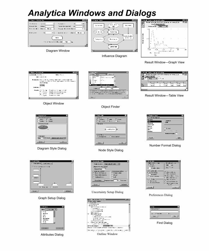
Analytica Windows and Dialogs
Diagram WindowInfluence Diagram
Result Window—Graph View
Object WindowObject Finder
Result Window—Table View
Diagram Style Dialog Node Style Dialog
Graph Setup Dialog
Uncertainty Setup Dialog
Number Format Dialog
Find Dialog
Preferences Dialog
Attributes Dialog Outline Window
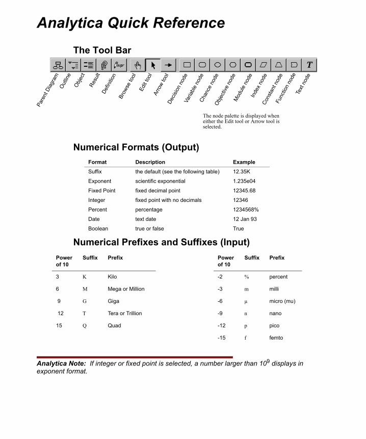
Analytica Quick ReferenceThe Tool Bar
Numerical Formats (Output)
Numerical Prefixes and Suffixes (Input)
Analytica Note: If integer or fixed point is selected, a number larger than 109 displays in exponent format.
Format Description ExampleSuffix the default (see the following table) 12.35K
Exponent scientific exponential 1.235e04
Fixed Point fixed decimal point 12345.68
Integer fixed point with no decimals 12346
Percent percentage 1234568%
Date text date 12 Jan 93
Boolean true or false True
Power of 10
Suffix Prefix Power of 10
Suffix Prefix
3 K Kilo -2 % percent
6 M Mega or Million -3 m milli
9 G Giga -6 µ micro (mu)
12 T Tera or Trillion -9 n nano
15 Q Quad -12 p pico
-15 f femto
Objec
t
Defin
ition
Resu
lt
Outlin
e
Brow
se to
olEd
it too
lAr
row
tool
The node palette is displayed when either the Edit tool or Arrow tool is selected.
Chan
ce n
ode
Varia
ble n
ode
Decis
ion n
ode
Objec
tive
node
Inde
x nod
e
Func
tion
node
Mod
ule n
ode
Cons
tant
nod
e
Pare
nt D
iagra
m
Text
node