An Introduction into Anomaly Detection UsingCUSUM

Dominik Dahlem

2015-11-24 Tue

Outline

1 Introduction

2 Anomaly Detection

3 Summary

Introduction

Who am I?

• Dominik Dahlem, Lead Data Scientist, Boxever dominik.dahlem@boxever.com http://ie.linkedin.com/in/ddahlem http://github.com/dahlem @dahlemd

Introduction

Anomaly Creation

Introduction

What is Anomaly Detection

• Find the problem before it affects businesses (especially SaaS)• But what is an anomaly?

• rare class mining• chance discovery• novelty detection• exception mining• noise removal

Introduction

Challenges

• What is normal behaviour…• … if normal behaviour keeps evolving?• … if the boundary between normal and anomolous behaviour is

imprecise?• What are we doing with noisy data…

• … if the notion of outliers differs across application domains?• Availability of training data

Introduction

Outlier Detection

480 500 520 540 560 580

−100

0

100Remove???

1 outliers <- function(x, s) {2 q <- quantile(x, probs=c(.25, .75), na.rm=T)3 iqr <- q[2] - q[1]4 idx <- which((x < (q[1]-s*iqr)) | (x > (q[2]+s*iqr)),5 arr.ind=T)6 return(idx)7 }

Introduction

Model-based Anomaly Detection

Anomaly Detection

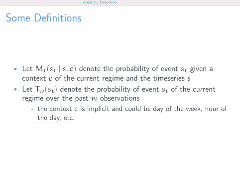
Some Definitions

• Let Mt(st | s, c) denote the probability of event st given acontext c of the current regime and the timeseries s

• Let Tw(st) denote the probability of event st of the currentregime over the past w observations

• the context c is implicit and could be day of the week, hour ofthe day, etc.

Anomaly Detection

The CUSUM Method2 (I)

• Let’s use the Gaussian kernel to estimate the densities1

T̂w(st) =1w

t−1∑`=t−w

1√2πσ

e−(s`−st)

2

2σ2 . (1)

M̂(st | s, c) =1k

∑`∈Φ(s,c)

1√2πσ

e−(s`−st)

2

2σ2 (2)

gauss <- function(st, s, sigmaSq) {Z <- 1/(sqrt(2 * pi * sigmaSq))bw <- 1/(2 * sigmaSq)n <- length(s)return(1/n * Z * sum(exp(-bw * (s - st)^2)))

}

1E. Gine (2002). “Rates of strong uniform consistency for multivariate kernel density estimators”. In: Annales de l?InstitutHenri Poincare (B) Probability and Statistics 38.6, pp. 907–921.

2E. S. Page (1954). “Continuous Inspection Schemes”. In: Biometrika 41.1/2, pp. 100–115.

Anomaly Detection

The CUSUM Method (II)

• Cumulative sum of the log-likelihood ratios

Rt = log[

T̂w(st)

M̂(st | s, c)

](3)

St = St−1 + Rt. (4)

• Raise alarm ifτ = inf{t | St − min

06k6t(Sk) > δ}. (5)

• The cumulative sum is zero if there is no anomaly

Anomaly Detection

CUSUM in R (I)

1 cusum <- function(params, training, s) {2 window <- params[1]3 slope <- params[2]4 df <- data.frame(t=seq(1,nrow(s)), g=rep(0, nrow(s)),5 R=rep(0, nrow(s)), Q=rep(0, nrow(s)),6 P=rep(0, nrow(s)), Sn=rep(0, nrow(s)),7 SnPrime=rep(0, nrow(s)), anomaly=rep(0, nrow(s)))89 for (t in (2+window):nrow(s)) {

10 s.subset <- s[(t-window):t,]11 cs <- unique(s.subset$c)12 training.subset <- subset(training, c %in% cs)

• Lines 2 and 3 are the tuning parameters• Line 9 steps over each time t

• Line 10 looks only at the last window observations• Line 11 selects the contexts within the chosen observations• Line 12: training set given the context(s)

Anomaly Detection

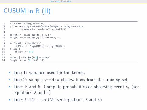
CUSUM in R (II)1 S <- var(training.subset$s)2 q.s <- training.subset$s[sample(length(training.subset$s),3 size=window, replace=T, prob=NULL)]45 df$P[t] <- gauss(s$s[t], q.s, S)6 df$Q[t] <- gauss(s$s[t], s.subset$s, S)78 if (df$P[t] & df$Q[t]) {9 df$R[t] <- -log(df$P[t]) + log(df$Q[t])

10 } else {11 df$R[t] <- 0.012 }13 df$Sn[t] <- df$Sn[t-1] + df$R[t]14 df$g[t] <- max(0, df$Sn[t])

• Line 1: variance used for the kernels• Line 2: sample window observations from the training set• Lines 5 and 6: Compute probabilities of observing event st (see

equations 2 and 1)• Lines 9-14: CUSUM (see equations 3 and 4)

Anomaly Detection

CUSUM in R (III)

1 df$SnPrime[t] <- (df$Sn[t]-df$Sn[t-window])/window2 if (df$SnPrime[t] < slope) {3 df$anomaly[t] <- 04 } else {5 df$anomaly[t] <- 16 }7 }8 return(df)9 }

• Line 1: compute the first derivative of the cumalative sum• The cumulative sum keeps growing• We would like to detect multiple anomalies

• Line 2: test whether we should raise an alarm

Anomaly Detection

CUSUM in Action

0 1,000 2,000 3,000 4,000 5,000 6,000

0

5

10

0 1,000 2,000 3,000 4,000 5,000 6,000

0

2,000

4,000

6,000

8,000

Summary

Also look at…

• https://github.com/twitter/AnomalyDetection• https://github.com/twitter/BreakoutDetection• https://github.com/robjhyndman/anomalous-acm• These slides and the R package is available at

• https://github.com/dahlem/cusum

Summary

Concluding…• We can detect anomalies if we can assume stationarity

• We modelled st − st−1 ≈ P(st − st−1 | c)

• CUSUM is sequential, so we can do anomaly detection easily inreal-time

• Types of anomalies• unusual noise• more noise• break down• sudden grow• peaks• no noise

• We cannot detect all kinds of anomalies with a single algorithm• use ensembles• handle outliers first?

BoxeverThank You!dominik.dahlem@boxever.com

Misclassification Rate

• Use this function to compute the classification error betweentraining and test set

1 classification.error <- function(x, training, s, ...) {2 df <- cusum(x, training, s, ...)3 return(1.0 - mean(df$anomaly == s$l))4 }

Parameter Tuning

• We use the CRAN package optimx to tune the parameters foranomaly detection

1 library(cusum)23 args <- commandArgs(trailingOnly = TRUE)45 training <- read.csv(args[1],6 header=F,7 col.names=c("c", "t", "s", "tot", "l"),8 stringsAsFactors=F)9 training$s <- as.numeric(training$s)

1011 s <- read.csv(args[2],12 header=F,13 col.names=c("c", "t", "s", "tot", "l"),14 stringsAsFactors=F)15 s$s <- as.numeric(s$s)1617 window <- as.integer(args[4])18 slope <- as.integer(args[5])1920 error <- optimx(c(window, slope), classification.error, training=training, s=s)21 print(error)

R Script

• Use this script to run CUSUM on the command-line1 library(cusum)23 args <- commandArgs(trailingOnly = TRUE)45 training <- read.csv(args[1],6 header=F,7 col.names=c("c", "t", "s", "tot", "l"),8 stringsAsFactors=F)9 training$s <- as.numeric(training$s)

1011 s <- read.csv(args[2],12 header=F,13 col.names=c("c", "t", "s", "tot", "l"),14 stringsAsFactors=F)15 s$s <- as.numeric(s$s)1617 window <- as.integer(args[4])18 slope <- as.integer(args[5])1920 df <- cusum(c(window, slope), training, s)21 write.table(df, args[3], row.names=F, sep=",", quote=F)