An Integrative Risk Evaluation Model

for Market Risk and Credit Risk

Shuji Tanaka∗

Yukio Muromachi†

Abstract

Not only financial institutions but all firms have their own portfolio consisting of various

financial assets. These portfolios are exposed to many kinds of risks, such as market risk, credit

risk, liquidity risk, operational risk, and so on. Basel Accord in 1998 prompted us to recognize

the importance of quantitatively evaluating these financial risks, and risk valuation models have

been developed, first for market risk and then credit risk. However, in these models, each risk is

evaluated separately, not integratively. Recently, Kijima and Muromachi [17] proposed a general

framework for the integrative evaluation of market risk (interest rate risk) and credit risk. In

this paper, we extend Kijima and Muromachi [17], and propose a framework to evaluate in a

integrative way market risk (not only interest rate risk but also stock price variation risk and

foreign exchange risk) and credit risk.

At the center of the framework are stochastic differential equations (SDEs) which describe

the dynamics of interest rate and default probability. We (i) run simulations with in the Monte-

Carlo method and generate scenarios based on these basic equations, (ii) calculate asset values

for a pre-specified future date (risk horizon) using no-arbitrage theory, and (iii) obtain the future

value of the portfolio by summing up all asset values. The main features of this framework are:

(i) we can take the correlation between the interest rate and the default probability into account,

(ii) the theoretical values of bonds derived in this setting are consistent with those observed in

the real market, (iii) we can incorporate the term structure of the default probability into the

model. Moreover, we can obtain the distribution of the portfolio or each asset value in the future,

and so we can calculate any risk measure (e.g. standard deviation, VaR, T-VaR etc.). Also, the

expected return can be computed, so the risk-return analysis can be made in a consistent way.

This framework enables us to construct many types of models by changing the basic SDEs.

We briefly present results for a Gaussian model, which is relatively easy to calculate.

Keywords: market risk, credit risk, hazard rates, conditional independence, VaR, risk contribu-

tions, SDEs

∗Executive Research Fellow, Financial Research Group. E-mail: tanaka@nli-research.co.jp†Quantitative Researcher, Financial Research Group. E-mail: muromati@nli-research.co.jp

1

Contents

1. Market Risk and Credit Risk 2

2. Desired Properties of Risk Valuation Models 3

3. Framework 4

3.1. Hazard rates . . . . . . . . . . . . . . . . . . . . . . . . . . . . . . . . . . . . . . . . 4

3.2. Basic stochastic differential equations . . . . . . . . . . . . . . . . . . . . . . . . . . 5

3.2.1. Interest rate processes and hazard rate processes . . . . . . . . . . . . . . . . 5

3.2.2. Stock price processes . . . . . . . . . . . . . . . . . . . . . . . . . . . . . . . . 6

3.2.3. Exchange rate processes . . . . . . . . . . . . . . . . . . . . . . . . . . . . . . 7

3.3. Conditional independence . . . . . . . . . . . . . . . . . . . . . . . . . . . . . . . . . 8

3.4. Valuation of present values . . . . . . . . . . . . . . . . . . . . . . . . . . . . . . . . 9

3.5. Distribution of future portfolio value . . . . . . . . . . . . . . . . . . . . . . . . . . . 11

3.6. Global structure of the model and general calculation procedures . . . . . . . . . . . 12

4. The Gaussian Model 14

4.1. Basic equations and their analytical solutions . . . . . . . . . . . . . . . . . . . . . . 14

4.1.1. Basic equations . . . . . . . . . . . . . . . . . . . . . . . . . . . . . . . . . . . 14

4.1.2. Analytical solutions . . . . . . . . . . . . . . . . . . . . . . . . . . . . . . . . 15

4.2. Term structure of hazard rates . . . . . . . . . . . . . . . . . . . . . . . . . . . . . . 16

4.3. Valuation formulas of simple instruments . . . . . . . . . . . . . . . . . . . . . . . . 17

4.3.1. Discount bond . . . . . . . . . . . . . . . . . . . . . . . . . . . . . . . . . . . 17

4.3.2. Fixed-rate coupon bond . . . . . . . . . . . . . . . . . . . . . . . . . . . . . . 17

4.3.3. Floating-rate coupon bond . . . . . . . . . . . . . . . . . . . . . . . . . . . . 18

4.3.4. Stock option . . . . . . . . . . . . . . . . . . . . . . . . . . . . . . . . . . . . 19

5. Numerical Examples 19

5.1. Preconditions . . . . . . . . . . . . . . . . . . . . . . . . . . . . . . . . . . . . . . . . 20

5.2. Results . . . . . . . . . . . . . . . . . . . . . . . . . . . . . . . . . . . . . . . . . . . . 22

5.2.1. Integrative evaluation of credit risk and market risk . . . . . . . . . . . . . . 22

5.2.2. Hedge of interest rate risk . . . . . . . . . . . . . . . . . . . . . . . . . . . . . 24

5.2.3. Risk/return analysis of each asset . . . . . . . . . . . . . . . . . . . . . . . . . 24

6. Concluding Remarks 24

1. Market Risk and Credit Risk

First, we briefly discuss market risk and credit risk as used in this paper.

2

The market risk of a portfolio consisting of many actively traded assets is measured through the

risk horizon (a prespecified time in the future to evaluate the risk), such as 1 day or 10 days. One

of the standard models used to measure the market risk today is RiskMetricsTM. In this model, the

return of each asset, or more precisely the risk factor, is assumed to have a multivariate Gaussian

distribution. This assumption is thought to be a good approximation.

We call the situation in which an issuer of a financial product cannot implement the contract a

default, and losses incurred by such default are said to represent credit risk. The credit risk includes

not only direct losses from cash flows that cannot be received due to the issuer’s default, but also

indirect losses when the asset value plunges because the possibility of the counterparty’s default

in the future rises sharply. Default, the origin of credit risk, is a binomial event in that it either

happens or not to happen. Hence, we cannot regard asset returns with credit risk as Gaussian

distributed. Moreover, because the typical horizon for credit risk is at least 1 year, we have to

distinguish the observed probability measure and the pseudo probability measure.1

Because there are many diffucult problems, we still don’t have a standard model of credit

risk measurement. Typical models are CreditMetricsTM and CREDITRISK+, but these can only

measure the credit risk, and the integration of market risk and credit risk had been made in a

tentative way. One of the reasons is that the theoretical framework of the integrative valuation of

multiple risks had not been constructed clearly until Kijima and Muromachi. In this paper, we

examine the framework of the integrative evaluation of the market risk and credit risk based on

Kijima and Muromachi [17].

Technical documents and textbooks on this issue can help in understanding typical models in

more detail.

2. Desired Properties of Risk Valuation Models

Based on the previous section, we list the desired propeties of an integrative valuation model of

market and credit risk.

(1) All assets are evaluated by one consistent method, such as no-arbitrage pricing.

(2) Portfolio effect, namely the effect due to the correlation among assets (especially in this case,

the correlation between two default probabilities or the correlation between the default prob-

ability and the interest rate) can be taken into consideration.

(3) The valuation is consistent with observable market prices.

(4) Term structure of interest rates and default rates are included in the framework. The frame-

work has the flexibility to incorporate empirical results into the model.

(5) The framework can properly treat the distributions of each asset return as assymetric and

non-Gaussian.

3

(6) Any distribution that we desire can be otained.

(7) The calculation load is not too heavy.

There are many sorts of assets, but the principles used to evaluate assets are not unified. For

instance, marketable assets traded actively in a market are evaluated by market value. On the

other hand, non-marketable assests such as loans are measured by contract value (book value).

Calculating each asset’s value in the simplest way makes it difficult to compute the risk of the

whole portfolio. In order to avoid this difficulty, we should adopt a unified measure to some extent.

There is agreement regarding the above conditions for integrative valuation models. But there

has been no actual model satisfying these conditions. However, Kijima and Muromachi [17] recently

proposed a framework to evaluate interest rate risk and credit risk in an integrative way and

provided a concrete model which satisfies most of the above conditions (we hereafter refer to this

model as the KM model). Tanaka and Muromachi [19] extended the KM model by including stock

price risk, mortality rate risk, and prepayment risk, and discussed its applicability to ALM of an

insurance company.

In this paper, we add stock price risk and foreign exchange risk to the KM model. Then we

overview integrated evaluation models and provide simple calculation results.2

This paper is organized as follows. In Section 3., we propose a framework of the integrated

evaluation model. In Section 4., we provide a concrete model based on this framework. In Section

5., we show numerical results of the model. Section 6. presents our conclusions.

3. Framework

In this section, we develop a general integrative framework to evaluate market and credit risk based

on the model Kijima and Muromachi prososed.

First, we explain the hazard rate which defines the default process. Then, we introduce the

structure of basic equations which describe the whole system, present the valuation method based

on this structure, and finally show a general procedure to calculate the distribution of future asset

prices.

Hereafter, we denote the observed probability measure by P , and consider the probability space

(Ω,F , P ). F = Ft; t ≥ 0 is a filtration generated by the stochastic system in this model. We

assume that there exists a unique risk-neutral probability measure P .

3.1. Hazard rates

Let t = 0 be the present time and τj denotes the default time of Firm j. We define hj(t) to

be its hazard rate of default under the observed probability measure P . The hazard rate hj(t)

represents the instantaneous rate that the default occurs at time t given no default before that

4

time. Therefore, hj(t) under condition τj > t is given by

hj(t) = limdt→0

Pt t < τj ≤ t + dt| τj > tdt

(1)

where Pt denotes the conditional probability measure of P given the information Ft. The hazard

rate can be thought of as the conditional intensity that a firm which does not default at time t will

default during the instaneaneous period (t, t + dt].

Suppose that hj(t) is a deterministic function of t. Then the probability that Firm j survives

after time T, T > t, is given by

P τj > T = exp

−∫ T

thj(u)du

. (2)

The default process of Firm j is characterized by the stochastic property of τj, but it is sufficient

to consider the term structure of hj(t), since we have the equation (2).

Next, we deal with the case that hj(t) is a random variable and Ft-measurable. If we know the

information FT , the survival probability is given by

PT τj > T = exp −Hj(t, T ) , Hj(t, T ) =∫ T

thj(u)du, (3)

where Hj(t, T ) is a cumulative hazard rate. On the other hand, the survival probability under the

condition τj > t is given by

Pt τj > T = Et

[exp

−∫ T

thj(u)du

], (4)

where Et[·] is the conditional expectation operator given the history Ft.

3.2. Basic stochastic differential equations

We now construct a model based on stochastic differential equations (SDEs) which describe the

behaviors of default-free interest rates, hazard rates, stock prices and exchange rates. In this section,

we first introduce these SDEs under the observed probability measure P . Next, we explain how to

construct the corresponding SDEs under the pseudo-probability measure, such as the risk-neutral

and the forward-neutral probability measure.

3.2.1. Interest rate processes and hazard rate processes

First, following Kijima and Muromachi [17], we introduce SDEs which interest rate and hazard

rate processes follow. This framework is basically the same as Jarrow and Turnbull [9], though the

expression is different.3

Suppose that there exist n firms. Let r(t) = h0(t) be the default-free spot rate and hj(t), j =

1, · · · , n, be the hazard rate of Firm j. We assume that the default-free spot rate and the hazard

rate processes under the observed probability measure P follow the system of SDEs:4

dr(t) = µ0(r(t), t)dt + σ0(r(t), t)dz0(t), t ≥ 0, (5)

dhj(t) = µj(h(t), t)dt + σj(h(t), t)dzj(t), t ≥ 0, j = 1, · · · , n, (6)

5

where (z0(t), z1(t), · · · , zn(t)) is a (n + 1)-dimensional standard Wiener process under P with cor-

relation

dzj(t)dzk(t) = ρjk(t)dt, j, k = 0, 1, · · · , n. (7)

We mentioned in the previous section that a hazard rate has its own term structure. By selecting

parameter values in (6) which fits the observed term structure, we can reflect results of empirical

analyses. We discuss this issue later.

Let β0(t) be the market price of risk associated with z0(t). Then for sufficiently large T ∗,

z0(t) = z0(t) +∫ t

0β0(u)du, 0 ≤ t ≤ T ∗ (8)

is a standard Wiener process under the risk-neutral probability measure P .5he SDE for r(t) under

P is given by

dr(t) = µ0(r(t), t)dt + σ0(r(t), t)dz0(t), 0 ≤ t ≤ T ∗, (9)

where

µ0(r(t), t) = µ0(r(t), t)− β0(t)σ0(r(t), t).

Next, we consider the hazard rates under P . By Artzner and Delbaen, when τj has its hazard

process hj(t) under the probability measure P , there exists a intensity process of τj under P which

is equivalent to P . Following Kijima [13], we assume that there exist a risk-premia adjustment

j(t) which is a deterministic function6 and satisfies

hj(t) = hj(t) + j(t), j = 1, · · · , n, (10)

where hj(t) is the hazard rate under the risk-neutral probability measure P . Note that the behavior

of the default-free spot rate and the hazard rate processes under the risk-neutral probability measure

P is determined by (6)C(7)C(9) and (10).

3.2.2. Stock price processes

As in Jarrow and Turnbull [9], we model stock price processes in addition to the processes in 3.2.1..7

Let Sj(t) denote the stock price of Firm j. We assume that Sj(t) follows the following SDE:8

dSj(t)Sj(t)

= (µs,j(t) + Xj(t)hj(t)) dt + σs,j(t)dzn+j(t) + dXj(t)

=

(µs,j(t) + hj(t)) dt + σs,j(t)dzn+j(t), t < τj,

−1, t = τj,j = 1, · · · , n, (11)

where Xj(t) = 1τj>tCand (z0(t), z1(t), · · · , zn(t), zn+1(t), · · · , z2n(t)) is a (2n + 1)-dimensional

standard Wiener measure under P with correlation

dzj(t)dzk(t) = ρjk(t)dt, j, k = 0, 1, · · · , 2n.

5T

6

In this case, under some regular conditions, there exists a market price of risk βn+j(t) such that

zn+j(t) = zn+j(t) +∫ t

0βn+j(u)du, j = 1, · · · , n

is a standard Wiener process under the risk-neutral probability measure P .9 Then, Sj(t) under P

follows the following SDE:

dSj(t)Sj(t)

=(r(t) + Xj(t)hj(t)

)dt + σs,j(t)dzn+j(t) + dXj(t)

=

(r(t) + hj(t)

)dt + σs,j(t)dzn+j(t), t < τj,

−1, t = τj,j = 1, · · · , n. (12)

3.2.3. Exchange rate processes

We further model foreign exchange rate processes as in Amin and Jarrow [1]. Let us consider a

default-free interest rate process, hazard rate processes, and stock price processes in the foreign

country. Let V (t) be the exchange rate, rf(t) the default-free spot rate, nf the number of firms,

τf,j the default time of Firm j and hf,j(t) its hazard rate, all in the foreign country. It is assumed

that they follow the following SDEs:10

drf(t) = µf,0(rf(t), t)dt + σf,0(rf(t), t)dzf,0(t), t ≥ 0, (13)

dhf,j(t) = µf,j(hf(t), t)dt + σf,j(hf(t), t)dzf,j(t), t ≥ 0, j = 1, · · · , nf , (14)dSf,j(t)Sf,j(t)

= (µfs,j(t) + Xf,j(t)hf,j(t)) dt + σfs,j(t)dzf,nf +j(t) + dXf,j(t)

=

(µfs,j(t) + hf,j(t)) dt + σfs,j(t)dzf,nf+j(t), t < τf,j ,

−1, t = τf,j ,j = 1, · · · , nf , (15)

dV (t)V (t)

= µV (t)dt + σV (t)dzV (t), (16)

where Xf,j(t) = 1τf,j>t, and z(t) = (z0(t), · · · , z2n(t), zf,0(t), · · · , zf,2nf(t), zV (t)) is a (2n + 2nf +

3)-dimensional standard Wiener measure under P with correlation

dzj(t)dzk(t) = ρjk(t)dt, j, k = 0, 1, · · · , 2n, (17)

dzf,j(t)dzf,k(t) = ρffjk (t)dt, j, k = 0, 1, · · · , 2nf , (18)

dzj(t)dzf,k(t) = ρfjk(t)dt, j = 0, 1, · · · , 2n, k = 0, 1, · · · , 2nf , (19)

dzj(t)dzV (t) = ρjV (t)dt, j = 0, 1, · · · , 2n, (20)

dzf,j(t)dzV (t) = ρfjV (t)dt, j = 0, 1, · · · , 2nf . (21)

As in the stock processes, µV (t) and σV (t) may depend on other random variables. Note that

dzV (t)dzV (t) = dt.

Next we consider the transformation of measure. We assume that for hf,j(t) and hf,j(t), the

relationship like (10) holds. From the calculation similar to the stock price process, we can derive

7

the following SDEs:

drf(t) = µf,0(rf(t), t)dt + σf,0(rf(t), t)dzf,0(t), 0 ≤ t ≤ T ∗, (22)

hf,j(t) = hf,j(t) + f,j(t), j = 1, · · · , nf , (23)dSf,j(t)Sf,j(t)

=(rf(t) + Xf,j(t)hf,j(t)

)dt + σfs,j(t)dzf,nf+j(t) + dXf,j(t)

=

(rf (t) + hf,j(t)

)dt + σfs,j(t)dzf,nf +j(t), t < τf,j ,

−1, t = τf,j ,j = 1, · · · , nf , (24)

dV (t)V (t)

= (r(t)− rf(t)) dt + σV (t)dzV (t), (25)

where z(t) = (z0(t), · · · , z2n(t), zf,0(t), · · · , zf,2nf(t), zV (t)) is a (2n+2nf +3)-dimensional standard

Wiener process under P and the correlation structure is the same as z(t).

We now have the framework we need to construct for the risk measure model. In summary,

the stochastic processes under the observed probability measure P follow (5)C(6)C(11)C(13)–(16)

and those under the risk-neutral probability measure P follow (9)C(10)C(12)C(22)–(25). The

correlation structure for z(t) and z(t) is given by (17)–(21).

This system of equations is so flexible that we can construct many types of models by changing

the structure of equations. We should note that Equation (12), (24) and (25) are necessary only

for the evaluation of stock/forex derivatives in the future time. For the portfolio consisting of only

stocks in the home and foreign countries (not including stock/forex derivatives), we only use (11),

(15) and (16) to calculate the future value, and (12), (24) and (25) are not needed.

3.3. Conditional independence

It is well known that the realization of the hazard rates hj(t) alone cannot determine the joint dis-

tribution of default times τj, since the joint distribution cannot be constructed from their marginal

distributions except in the independent case. Hence, a further assumption is necessary for our

purpose. In our model, we assume that τj are conditionally independent given the realization of

the underlying stochastic processes.

Let Pt τ1 > t1, · · · , τn > tn , tj ≥ t, be the joint distribution of default times. The conditional

independence means that given FT where T ≥ maxj tj , the default times τj mutually independent,

i.e.,

PT τ1 > t1, · · · , τn > tn =n∏

j=1

PT τj > tj . (26)

By taking the unconditional expectation for both sides in (26), we then obtain

P τ1 > t1, · · · , τn > tn = E

n∏j=1

PT τj > tj = E

exp

−n∑

j=1

∫ tj

0hj(u)du

, (27)

8

where we have used Equation (3). We can take the correlation structure of hj(t) into consideration

when we assume the conditional independence in contrast to the ordinary independence, i.e.

P τ1 > t1, · · · , τn > tn =n∏

j=1

E

[exp

−∫ tj

0hj(u)du

]holds.

The reader who want to understand the conditional independence for more detail should consult

the latter section which treats the simulation.

3.4. Valuation of present values

In this subsection, we briefly touch upon the general issue on the valuation of financial products,

and then mention the valuation of defaultable discount bonds. The idea is based on the framework

of Jarrow and Turnbull [9].

According to the no-arbitrage pricing theory in the finance literature, pricing of derivatives can

be done by the risk-neutral method or the forward-neutral method. Consider a contingent claim

which generates a cash flow X at the maturity date T . The price of this claim at time t, t < T ,

p(t, T ), can be written as

p(t, T ) = Et

[e−∫ T

tr(s)dsX

]= v0(t, Y )ET

t [X ], (28)

where Et[·] is a conditional expectation operator under the risk-neutral probability measure, ETt [·]

is a conditional expectation operator under the forward-neutral probability measure, and v0(t, T ) is

the price at time t of discount bond free from default. For example, when the claim is an European

call option of Stock j, we can calculate the price by substituting

X = (Sj(T ) − K)+,

where Sj(T ) is the stock price at the maturity date T , K is the exercise price, and (A)+ = max(A, 0).

We provide a concrete example of a defaultable discount bond in order to make clear the idea

of this pricing method. Consider the i-th discount bond which Firm j issued. For simplicity, we

assume that a holder of the bond reveives $1 at the maturity T ji if the default does not occur until

T ji , and $δj if the default occurs. This assumption is consistent with Jarrow and Turnbull [9], when

we consider the case that the bond holder receives δjv0(τj, Tji ) at the default time τj when the

default occurs. Our assumption can make the problem fairly simple because the future cash flow

is not explicitly dependent on τj.

The cash flow of the bond holder at the maturity date Tj can be expressed as X = δj1τj≤T ji

+

1τj>Tji

. Let vj(t, T ) denote the timet price of the defaultable discount bond with maturity T

issued by Firm j. Then, vj(t, T ) is given by

vj(t, Tji ) = Et

[exp

−∫ T j

i

tr(u)du

δj1τj≤T j

i + 1τj>T j

i ]

= δjv0(t, Tji ) + (1 − δj)Et

[e−H0(t,T j

i )−Hj (t,T ji )], (29)

9

where

v0(t, T ) = Et

[e−H0(t,T )

],

H0(t, T ) =∫ T

th0(u)du,

Hj(t, T ) =∫ T

thj(u)du, j = 0, 1, · · · , n.

If r(t) and hj(t) are independent, Equation (29) coincides

vj(t, Tji ) = v0(t, T

ji )[δj + (1 − δj)Pt

τj > T j

i

],

which Jarrow and Turnbull [9] obtained. Here, Ptτj > T ji is the survival probability of Firm

j under the risk-neutral probability measure P conditional on Ft. When r(t) and hj(t) are not

independent, we have to take the correlation between H0(t, Tji ) and Hj(t, T

ji ) into account in

calculating the expectation.

The use of the forward-neutral probability measure makes the calculation simpler. Let PT

denote the forward-neutral probability measure. Then, the defaultable discount bond price is given

by

vj(t, Tji ) = v0(t, T

ji )ET

ji

t

[δj1τj≤T j

i + 1τj>T j

i ]

= v0(t, Tji )[δj + (1 − δj)P

T ji

t

τj > T

ji

], (30)

where PTt denotes the conditional probability measure given Ft under PT , whichi is equivalent to

the risk-neutral probability measure P . We need not consider the correlation between the interest

rate and the hazard rate in this method.

In (30), the survival probability PT j

it can be calculated as follows. Let hT

j (t) be the risk-adjusted

hazard rate process under PT , and hj(t) be the observed hazard rate process. We assume that

there exist a risk premia adjustment Tj (t) satisfying

hTj (t) = hj(t) + T

j (t) (31)

In general, each risk premia adjusment Tj (t) may depend on the whole hisory and the maturity

T . However, we assume in our framework that Tj (t) is a deterministic function of time t and inde-

pendent of the maturity, and so we can denote it by j(t). Then, the marginal survival probability

under PT j

it is given by

PT j

it τj > T = E

T ji

t

[exp

−∫ T

th

T ji

j (u)du

]= Pt τj > TLj(t, T ), t ≤ T ≤ T

ji , (32)

Lj(t, T ) = exp

−∫ T

tj(u)du

.

At time t, we can observe the value of v0(t, s), vj(t, s) and Ptτj > s, s ≥ t in the market.

Therefore, the risk premia adjusment Tj (t) can be calculated as

j(s) = − ∂

∂slog

1

Ptτj > s(

vj(t, s)v0(t, s)

− δj

), s ≥ t. (33)

10

β0(t), the market price of risk of z0(t), also can be estimated by the term structure of v0(t, s). We

deal with this issue later.

When we obtain the functional form of Tj (t) = j(s), we also obain hT

j (s), the hazard rate

under PT . Hence, we can compute other prices of assets with the credit risk by the forward-neutral

method. In general, we can evaluate asset prices more easily by the forward-neutral method than

by the risk-neutral method. We have to take notice that the forward-neutral probability measure

PT depends on the maturity T .

Thanks to (33), j(s) can be obtained and is consistent with the market data. Since any market

price includes all risks evaluated by the market other than interest rate risk and credit risk, j(s)

obtained in this way comprehends effects by these risks. Using this j(s) enables us to include

implicitly the effect of other risks of the future in the model. This j(s) can be said to be an very

effective tool when we want to measure multiple risks in a integrative way, which is consistent with

observable market values.

3.5. Distribution of future portfolio value

Let us consider the distribution of the future value of the portfolio which consists of discount bonds

and stocks.

In what follows, we denote the risk horizon by T, T > t and suppose that the our model satisfies

the assumptions specified so far. Then the price at the risk horizon T of the i-th defaultable

discount bond issued by Firm j with maturity T ji is given from (30) and (32) by

vj(T, Tji ) =

v0(T, T ji )[δj + (1 − δj)PT

τj > T j

i

Lj(T, T j

i )], τj > T

v0(T, Tji )δj , τj ≤ T

= v0(T, T ji )[δj + (1 − δj)PT

τj > T j

i

Lj(T, T j

i )1τj>T]. (34)

Here vj(T, T ji ) is a random variable dependent on v0(T, T j

i )CPT

τj > T j

i

and τj. On the other

hand, the stock price issued by Firm j is writtem from (11) as

Sj(T ) =

Sj(t) +∫ Tt Sj(u) (µs,j(u) + hj(u))du +

∫ Tt Sj(u)σs,j(u)dzn+j(u), τj > T,

0, τj ≤ T,

=

[Sj(t) +

∫ T

tSj(u) (µs,j(u) + hj(u)) du +

∫ T

tSj(u)σs,j(u)dzn+j(u)

]1τj>T. (35)

From (34) and (35), the portfolio value at the risk horizon T is given by

π(T ) =n∑

j=0

Nj∑i=1

wji v0(T, T j

i )[δj + (1 − δj)PT

τj > T j

i

Lj(T, T j

i )1τj>T]

+wjs

[Sj(t) +

∫ T

tSj(u) (µs,j(u) + hj(u)) du +

∫ T

tSj(u)σs,j(u)dzn+j(u)

]1τj>T

)(36)

where wjs denotes the number of Sj(t) which the portfolio has, wj

i denotes the number of vj(t, Tji ),

and Nj is the number of discount bonds issued by Firm j (or the default-free discount bonds for

j = 0).

11

3.6. Global structure of the model and general calculation procedures

After obtaining the joint distribution of v0(T, T ji ), PT

τj > T j

i

and τj at T from the basic SDEs,

we can calculate by (36) the distribution of the portfolio in principle. However, it seems very difficult

to obtain analytically the distribution of the portfolio even when v0(T, T ji ) and PT

τj > T j

i

follow

tractable distributions, because Equation (36) includes the indicator function 1A. Hence, in this

case, we compute the distribution of the portfolio by Monte-Carlo simulation.

We show the brief scheme in Figure 1. As mentioned above, this framework is flexible in

setting the models of default-free interest rates, hazard rates, stock prices, foreign exchange rates.

Therefore, we can flexibly construct a variety of models by changing the structure of SDEs.

As in the above procedure, we have to use the Monte-Carlo simulation in a nested way to

obatain the distribution of the future value except for some special settings. That is, the generation

of scenarios until the risk horizon is the first-step simulation and the evaluation of each scenario at

the risk horizon is the second-step. When many scenarios are necessary at each step simulation,

it takes a long time to compute and this framework becomes practically unrealistic. We show a

Gaussian model which is an extention of Kijima and Muromachi [17] and makes the computation

time remarkably shorter.

12

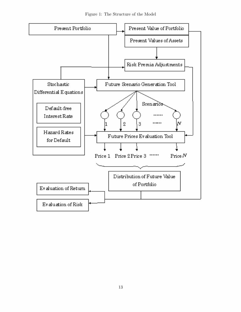
Figure 1: The Structure of the Model

13

4. The Gaussian Model

The Gaussian model enables us to obtain the closed-form solutions and save much time in calcu-

lating values.

4.1. Basic equations and their analytical solutions

4.1.1. Basic equations

Let t = 0 be the present time. We assume here that in our model the basic equations under the

observed probability measure P follow the system of SDEs

dr(t) = (b0(t) − a0r(t)) dt + σ0dz0(t), t ≥ 0, (37)

dhj(t) = (bj(t) − ajhj(t)) dt + σjdzj(t), t ≥ 0; j = 1, · · · , n, (38)

dSj(t)Sj(t)

=

µs,jdt + σs,jdzn+j(t), t < τj,

−1, t ≥ τj,j = 1, · · · , n, (39)

drf(t) = (bf,0(t) − af,0rf(t)) dt + σf,0dzf,0(t), t ≥ 0, (40)

dhf,j(t) = (bf,j(t) − af,jhf,j(t)) dt + σf,jdzf,j(t), t ≥ 0; j = 1, · · · , nf , (41)

dSf,j(t)Sf,j(t)

=

µfs,jdt + σfs,jdzf,nf +j(t), t < τf,j ,

−1, t ≥ τf,j ,j = 1, · · · , nf , (42)

dV (t)V (t)

= µV dt + σV dzV (t). (43)

where a0, aj, af,0, af,j , σ0, σj, σf,0, σf,j , σs,j, σfs,j, σV are non-negative constants, µs,j , µfs,j, µV

are constants, b0(t), bj(t), bf,0(t), bf,j(t) are deterministic function of time t and the correlations

between zj(t) are constants. Let us further assume that the market price of risk β0(t), βf,0(t) associ-

ated with z0(t), zf,0(t) and the risk-premia adjustments j(t), f,k(t) associated with hj(t), hf,k(t), j =

1, · · · , n, k = 1, · · · , nf , are deterministic functions of time. Then, each variable follows under the

risk-neutral probability P the following SDEs:

dr(t) = (φ0(t) − a0r(t))dt + σ0dz0(t), t ≥ 0, (44)

hj(t) = hj(t) + j(t), j = 1, · · · , n, (45)

dSj(t)Sj(t)

=

[r(t) + hj(t)

]dt + σs,jdzn+j(t), t < τj,

−1, t ≥ τj,j = 1, · · · , n, (46)

drf(t) = (φf,0(t) − af,0rf (t)) dt + σf,0dzf,0(t), t ≥ 0, (47)

hf,j(t) = hf,j(t) + f,j(t), j = 1, · · · , nf , (48)

dSf,j(t)Sf,j(t)

=

[rf(t) + hf,j(t)

]dt + σfs,jdzf,nf +j(t), t < τf,j ,

−1, t ≥ τf,j ,j = 1, · · · , nf , (49)

dV (t)V (t)

= [r(t)− rf(t)] dt + σV dzV (t). (50)

Note that the default-free interest rate described as (44) is an extended Vasicek model which

appeared in Hull and White. According to Inui and Kijima [8], the function φj(t) can be obtained

14

so that the model is consistent with the current term structure of the default-free interest rates

observed in the market. That is to say,

φ0(t) = a0f0(0, t) +∂

∂tf0(0, t) +

σ20

2a0

(1 − e−2a0t

), (51)

φf,0(t) = af,0ff,0(0, t) +∂

∂tff,0(0, t) +

σ2f,0

2af,0

(1 − e−2af,0t

), (52)

where f0(0, t), ff,0(0, t) denote the forward rate of the default-free discount bond. The market

prices of risk associated with z0(t) and zf,0(t) are given by

β0(t) =b0(t)− φ0(t)

σ0, βf,0(t) =

bf,0(t) − φf,0(t)σf,0

,

respectively.

The hazard rate processes under P and P are formally the same as extended Vasicek model.

From (38) and (45) and the assumption of the risk-premia adjustments, we obtain

dhj(t) =(φj(t) − ajhj(t)

)dt + σjdzj(t), j = 1, · · · , n, (53)

φj(t) = bj(t) + ajj(t) +dj(t)

dt.

Following Kijima [14], φj(t) can be computed so that the model is consistent with the current term

structure of the defaultable interest rates observed in the market. That is to say, φj(t) is given by

φj(t) = ajgj(0, t) +∂

∂tgj(0, t) +

σ2j

2aj

(1 − e−2ajt

)+ρ0jσ0σj

(1 − e−a0t

a0+

e−a0t − e−(a0+aj)t

aj

), (54)

where

gj(t, T ) = − ∂

∂Tlog[vj(t, T )v0(t, T )

− δj

].

The market price of risk associated with zn+j(t) is given by

βn+j(t) =µs,j − r(t)− hj(t)

σs,j.

Other market prices of risk associated with zf,nf +j(t), zV (t) are given in the same way as above.

4.1.2. Analytical solutions

hj(t) in (38) and its cumulative hazard rates are easily solved as

hj(t) = hj(0)e−ajt +∫ t

0bj(u)e−aj(t−u)du + σj

∫ t

0e−aj (t−u)dzj(u), t ≥ 0,

Hj(t, T ) = hj(t)Bj(t, T ) +∫ T

tbj(u)Bj(u, T )du + σj

∫ T

tBj(u, T )dzj(u), 0 ≤ t ≤ T,

15

where

Bj(t, T ) =1− e−aj(T−t)

aj.

Here hj(t) and Hj(t, T ) follow Gauss-Markov processes. Their means, variances and covariance are

given by

mj(t) = E[hj(t)] = hj(0)e−ajt +∫ t

0bj(u)e−aj(t−u)du,

s2j (t) = V [hj(t)] =

σ2j

2aj

(1 − e−2ajt

),

Mj(t, T ) = E[Hj(t, T )] = hj(t)Bj(t, T ) +∫ T

tbj(u)Bj(u, T )du,

S2j (t, T ) = V [Hj(t, T )] =

σ2j

a2j

[(T − t) − 2

1 − e−aj (T−t)

aj+

1 − e−2aj(T−t)

2aj

],

sjk(t) = Cov[hj(t), hk(t)] =ρjkσjσk

aj + ak

(1− e−(aj+ak)t

),

Sjk(t, T ) = Cov[Hj(t, T ), Hk(t, T )]

=ρjkσjσk

ajak

[(T − t) − 1 − e−aj (T−t)

aj− 1 − e−ak(T−t)

ak+

1 − e−(aj+ak)(T−t)

aj + ak

],

Cjk(t) = Cov[hj(t), Hk(0, t)] =ρjkσjσk

aj

[1− e−ajt

aj− 1 − e−(aj+ak)t

aj + ak

].

We can obtain the solution of (37)C(40)C(41)C(44)C(47)C(53) in the same manner as that of (38).

Next, we consider the stock price and the exchange rate. The solution of (39) is written as

Sj(t) =[Sj(0) exp

(µs,j − 1

2σ2

s,j

)t + σs,jzj(t)

]1τj>t, t ≥ 0, j = 1, · · · , n.

We can solve (42) in the same manner. Also, the solution of (43) is given by

V (t) = V (0) exp(

µV − 12σ2

V

)t + σV zV (t)

, t ≥ 0.

Finally, (46), (49) and (50) are also solvable. For instance, the solution of (46) is given by

Sj(t) = Sj(0) exp∫ t

0(r(s) + hj(s))ds − 1

2σ2

s,jt + σs,j zs,j(t)

= Sj(0) exp

H0(0, t) + Hj(0, t)− 12σ2

s,jt + σs,j zs,j(t)

.

Sj(t) is a random variable dependent on (H0(0, t), Hj(0, t), zs,j(t)), which follows a 3-dimensional

multivariate Gaussian distribution. These variables are only used in the evaluation of stock/foreign

exchange derivatives and do not appear explicitly.

4.2. Term structure of hazard rates

We provide a concrete method which comprehends empirical results on the term structure of default

probabilities.

16

In this model, we assume that the term structure of the hazard rates follows the Weibull

distribution11 with three parameters

mj(t) = E [hj(t)] = λjγj (t + mj)γj−1 , t ≥ 0, λj, γj > 0, mj ≥ 0. (55)

The parameters λj, γj, mj in (55) can be estimated from default data. Note that in this case, we

have

bj(t) =∂

∂tmj(t) + ajmj(t) = λjγj [γj − 1 + aj(t + mj)] (t + mj)

γj−2

from the solution of hj(t).

4.3. Valuation formulas of simple instruments

We present some solutions of prices of simple products.

4.3.1. Discount bond

The time t price of the default-free discount bond is given by

v0(t, T ) = A0(t, T )e−B0(t,T )r(t),

where

Aj(t, T ) = exp

12S2

j (t, T )−∫ T

tφj(u)Bj(u, T )du

, j = 0, 1, · · · , n.

The time t price of the defaultable discount bond with constant recovery rate δj is given from (29)

by

vj(t, Tji ) = v0(t, T

ji )[δj + (1 − δj)Aj(t, T

ji )eS0j(t,T j

i )e−Bj (t,T ji )hj(t)1τj>t

]= v0(t, T

ji )[δj + (1 − δj)Pt

τj > T j

i

Lj(t, T

ji )eS0j(t,T

ji )1τj>t

]The forward-neutral method makes the expression of the price simpler. The time t price of the

defaultable discount bond with recovery rate δj is given from (30) and (32) by

vj(t, Tji ) = v0(t, T

ji )[δj + (1 − δj)Lj(t, T )Pt

τj > T j

i

]. (56)

4.3.2. Fixed-rate coupon bond

The time t price of the defaultable coupon bond with recovery rate δj is given by

pj(t, T; C, δ) = vj(t, tM ; δ) + CM∑

j=1

vj(t, tj; δ),

where C is the coupon rate, tM is the maturity of the bond, and T = (t1, t2, . . . , tM), tj > t, j =

1, . . . , M is the coupon payment dates. Especially, the time t price of the default-free coupon bond

is given by

p0(t, T; C) = v0(t, tM) + CM∑

j=1

v0(t, tj). (57)

17

4.3.3. Floating-rate coupon bond

We consider the following floating-rate coupon bond. Let T = (t1, t2, . . . , tM), tj > t, j = 1, . . . , M

be the coupon payment dates, tM be the maturity date, and δ be the recovery rate. The coupon

rate in the period (tj , tj+1] is C(tj , q) and C(t, q) is

C(t, q) = αR(t, q) + β, R(t, q) = − log v0(t, t + q)q

, q > 0,

where α and β are constants, and R(t, q) denotes the default-free discount yield with the maturity

q at time t. Then, we have the following relation,

C(t, q) = α′r(t) + β′,

where

α′ =α

qB0(t, t + q), β′ = β − α

qlog A0(t, t + q) (58)

t0 < t denote the latest coupon date before t. If t0 = t, the bond price is supposed to be ex-

divindend.

When the bond is default-free, then the time t price of the floating-rate bond is given by

p0(t, T; α, β) = v0(t, tM) + C(t0, q)(t1 − t0)v0(t, t1) +M∑

j=2

p0(t, tj−1, tj; α′, β′), (59)

where C(t0, q) is the last coupon rate observable at t0 ≤ t, and

p0(t, t1, t2; α′, β′) = p0(t, t1, t2; α, β, q)

denotes the price of the default-free discount bond whose holder receives C(t1, q)(t2−t1) at t2, t2 >

t1. Simple algebra yields

p0(t, t1, t2; α′, β′) = (t2 − t1)v0(t, t2)[β′ + α′

r(t)e−a0(t1−t) +

∫ t1

tφ0(u)e−a0(t1−u)du

−σ20

a20

(1 − e−a0(t1−t) − e−a0(t2−t1) − e−a0(t1+t2−2t)

2

)]Next, when the floating-rate bond is defaultable, then the time t price of the bond is given by

pj(t, T; α, β, δ) = vj(t, tM ; δ) + C(t0, q)(t1 − t0)vj(t, t1; δ) +M∑

j=2

pj(t, tj−1, tj; α′, β′, δ),

where

pj(t, t1, t2; α′, β′, δ) = pj(t, t1, t2; α, β, q, δ)

denotes the price of the defaultable discount bond whose holder receives C(t1, q)(t2− t1) at t2, t2 >

t1. By some calculations, we obtain

pj(t, t1, t2; α′, β′, δ) = p0(t, t1, t2; α′, β′)[δ + (1 − δ)P t2

t τj > t2]

−(1 − δ)(t2 − t1)α′v0(t, t2)P t2t τj > t2

×ρ0jσ0σj

aj

1 − e−a0(t1−t)

a0− e−aj (t2−t1) − e−a0(t1−t)−aj(t2−t)

a0 + aj

.

18

4.3.4. Stock option

The time t price of the European call stock option of Firm j with maturity T > t and excercise

price K > 0 is given by

c(t, T ; K) = Sj(t)Φ(z)− Kvj(t, T ; δj = 0)Φ(z − σX),

where

z =log(

Sj(t)Kvj(t,T ;δj=0)

)σX

+12σX ,

σX =

(σ2

0

∫ T

tB2

0 (u, T )du + σ2j

∫ T

tB2

j (u, T )du + σ2s,j(T − t)

+2σ0σjρ0j

∫ T

tB0(u, T )Bj(u, T )du + 2σ0σs,jρ0,n+j

∫ T

tB0(u, T )du

+2σjσs,jρj,n+j

∫ T

tBj(u, T )du

)12

,

and vj(t, T ; δj = 0) is the time t price of the discount bond issued by Firm j with maturity T with

recover rate zero. We can obtain by some calculation

log vj(t, T ; δj = 0) = −r(t)B0(t, T )−∫ T

tφ0(u)B0(u, T )du

−hj(t)Bj(t, T )−∫ T

tφj(u)Bj(u, T )du

+12σ2

0

∫ T

tB2

0(u, T )du +12σ2

j

∫ T

tB2

j (u, T )du

+σ0σjρ0j

∫ T

tB0(u, T )Bj(u, T )du.

The time t price of the European put stock option of Firm j with maturity T > t and excercise

price K > 0 is given by

p(t, T ; K) = Kvj(t, T ; δj = 0)Φ(−z + σX) − S(t)Φ(−z)

5. Numerical Examples

We briefly provide results on the distribution at the risk horizon of the portfolio consisting of n

bonds. The risk horizon is set to be 1 year.

Before proceeding, we briefly explain the risk measures we use below.

• VaR: The difference between the expected value of the portfolio and 100(1 − α)-percentile

point at the risk horizon. This can be obtained from the distribution of each price at the risk

horizon.

• T-VaR: The difference between the expected value of the portfolio and the average below

100(1− α)-percentile point at the risk horizon.

19

• RC (risk contribution): Risk quantity of each asset which is allocated based on the risk

quantity of the whole portfolio (e.g. standard deviation, VaR, T-Var). This can be obtained

by simulation results. The summation of each asset RC is equal to RC of the portfolio.

• RC ratio: The discounted present value of RC.

• RC measure: The proportion of RC ratio to the expected ruturn. This measure is used for

return/risk analysis.

Note that RC, RC ratio and RC measure are not commonly used terminologies.

5.1. Preconditions

The preconditions are basically the same as Kijima and Muromachi [17]. Table 1 shows the attri-

butions of each bond (credit rating, face value, maturity, coupon rate, discovery rate).

Table 1: Attribution of each bond of the portfolioFirm Credit rating Face value Maturity (years) Coupon rate Recovery rate

A Aaa 7 3 7.25% 0

B Aa 1 4 8.0% 0

C A 1 3 8.25% 0

D Baa 1 4 9.0% 0

E Ba 1 3 9.25% 0

F B 1 6 10.25% 0

G GB 1 2 7.0% 0

H A 10 8 9.5% 0

I Ba 5 2 9.0% 0

J A 3 2 8.0% 0

K A 1 4 8.5% 0

L A 2 5 8.75% 0

M B 0.6 3 9.75% 0

N B 1 5 10.25% 0

O B 3 2 9.5% 0

P B 2 4 10.0% 0

Q Baa 1 6 9.5% 0

R Baa 8 5 9.25% 0

S Baa 1 3 8.75% 0

T Aa 5 5 8.25% 0

All coupon payments are done every six months and the cash flow generated during the two

payment dates are assumed to be invested at a risk-free rate. Credit ratings consist of 6 grades

20

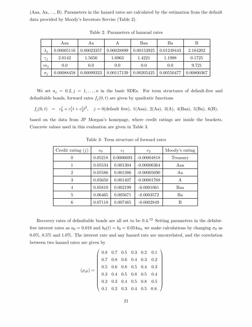
(Aaa, Aa,. . ., B). Parameters in the hazard rates are calculated by the estimation from the default

data provided by Moody’s Investors Servise (Table 2).

Table 2: Parameters of hazarad rates

Aaa Aa A Baa Ba B

λj 0.00005116 0.00023357 0.00028899 0.00153925 0.01249443 2.164202

γj 2.0142 1.5656 1.6963 1.4221 1.1998 0.1725

mj 0.0 0.0 0.0 0.0 0.0 9.721

σj 0.00088458 0.00099323 0.00117139 0.00205425 0.00550477 0.00800367

We set aj = 0.2, j = 1, . . . , n in the basic SDEs. For term structures of default-free and

defaultable bonds, forward rates fj(0, t) are given by quadratic functions

fj(0, t) = cj0 + cj

1t + cj2t

2, j = 0(default free), 1(Aaa), 2(Aa), 3(A), 4(Baa), 5(Ba), 6(B),

based on the data from JP Morgan’s homepage, where credit ratings are inside the brackets.

Concrete values used in this evaluation are given in Table 3.

Table 3: Term structure of forward rates

Credit rating (j) c0 c1 c2 Moody’s rating

0 0.05218 0.0006693 -0.00004818 Treasury

1 0.05534 0.001304 -0.00006364 Aaa

2 0.05586 0.001386 -0.00005690 Aa

3 0.05650 0.001407 -0.00001768 A

4 0.05810 0.002199 -0.0001061 Baa

5 0.06465 0.005671 -0.0003572 Ba

6 0.07118 0.007465 -0.0002849 B

Recovery rates of defaultable bonds are all set to be 0.4.12 Setting parameters in the defalut-

free interest rates as a0 = 0.018 and b0(t) = b0 = 0.054a0, we make calculations by changing σ0 as

0.0%, 0.5% and 1.0%. The interest rate and any hazard rate are uncorrelated, and the correlation

between two hazard rates are given by

(ρjk) =

0.8 0.7 0.5 0.3 0.2 0.1

0.7 0.8 0.6 0.4 0.3 0.2

0.5 0.6 0.8 0.5 0.4 0.3

0.3 0.4 0.5 0.8 0.5 0.4

0.2 0.3 0.4 0.5 0.8 0.5

0.1 0.2 0.3 0.4 0.5 0.8.

21

The order is as Aaa, Aa, A, Baa, Ba, B, both in column and row. The diagonal elements are all

0.8, which is the correlation between two firms in the same rating. We use 5000 sample paths.

5.2. Results

5.2.1. Integrative evaluation of credit risk and market risk

The distribution of the portfolio at time T = 1 is shown in Table 2. The result (a) is when we

only consider the credit risk (σ0 = 0.00%), and (b) is the result when we consider the credit risk

and the market risk integratively (σ0 = 1.0%). The distribution in (a) is multimodal. The highest

peak is for the case that no default occurs, and the left three peaks next to the highest are for the

case when one of the assets F, N, O, P, all of which belong to rating G, defaults. There are some

peaks left to these three correspond to many kinds of defaults, such as the default of a bond with

a large face value, multiple assets default, and so on. This multimodality is one of notable features

of the credit risk.13 In (b), the shape of the distribution is unimodal, since peaks overlap due to

the interest rate risk. Figure 4 presents risk measures for comparison. These results imply that the

interest rate risk should not be ignored in the calculation of future distribution.

In Case (c), stocks are added to the portfolio (σ0 = 1.0%). The stocks added consist of those

of Firms B, D, F, H, J and L. All initial prices are 2 and µS = 0.2, σS = 0.1. Any two stocks

are uncorrelated. In this case, the distribution has a fatter tail than that in (b). This means that

adding stocks to a portfolio which consists only of bonds exposes the firm to much more market

risks and also that the credit exposure due to specific firms becomes remarkable. That is why

VaR and T-VaR, which is greatly affected by the credit risk, increases in this case even when the

addition of stocks to the portfolio is not too much.

22

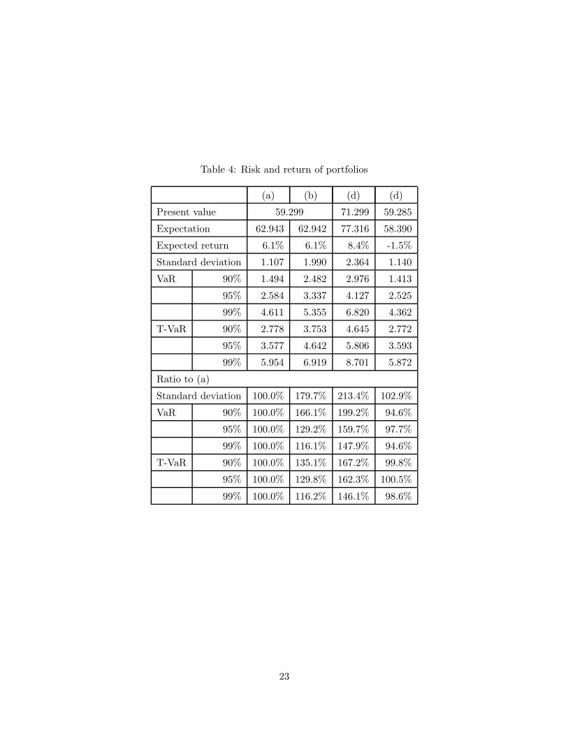
Table 4: Risk and return of portfolios

(a) (b) (d) (d)

Present value 59.299 71.299 59.285

Expectation 62.943 62.942 77.316 58.390

Expected return 6.1% 6.1% 8.4% -1.5%

Standard deviation 1.107 1.990 2.364 1.140

VaR 90% 1.494 2.482 2.976 1.413

95% 2.584 3.337 4.127 2.525

99% 4.611 5.355 6.820 4.362

T-VaR 90% 2.778 3.753 4.645 2.772

95% 3.577 4.642 5.806 3.593

99% 5.954 6.919 8.701 5.872

Ratio to (a)

Standard deviation 100.0% 179.7% 213.4% 102.9%

VaR 90% 100.0% 166.1% 199.2% 94.6%

95% 100.0% 129.2% 159.7% 97.7%

99% 100.0% 116.1% 147.9% 94.6%

T-VaR 90% 100.0% 135.1% 167.2% 99.8%

95% 100.0% 129.8% 162.3% 100.5%

99% 100.0% 116.2% 146.1% 98.6%

23

5.2.2. Hedge of interest rate risk

Next, we provide an example to hedge the interet rate risk in the portfolio consisting of 20 bonds

as above by using interest-rate swap. The swaps which we use are the following.

• Swap A: Maturity 2 years, coupon payment every 6 months, 6-month floating rate and fixed

rate (5.28%), notational principal 30.4

• Swap B: Maturity 4 years, coupon payment every 6 months, 6-month floating rate and fixed

rate (5.32%), notational principal 30.0

• Swap C: Maturity 6 years, coupon payment every 6 months, 6-month floating rate and fixed

rate (5.35%), notational principal 20.0

The present value of all these swaps is nearly zero and the duration of the portfolio equals

approximately zero when these swaps are added to the original portfolio.

Table 3 shows the distributions of the portfolio to which Swap A, Swap B and Swap C are added

in order. Swaps are evaluated as default-free. Figure 4 shows the result for Case (d), in which all

swaps are included in the portfolio. Table 3 and 4 show clearly the effect of hedging by interest-rate

swaps. In Case (d) where the duratio is nearly zero, the shape is similar to (a) where the interest

rate risk is not taken into account. This implication can also be seen from risk measures of (d).

5.2.3. Risk/return analysis of each asset

Finally, we provide results on the risk/return analysis of each asset.

Figure 4 shows the RC (risk contribution) of 95% T-VaR and the present values of RC. Com-

paring RC with T-VaR of each asset calculated separately, RC is half the T-VaR in average, 10%

for some case, because of the diversification effect. Hereinafter, we use RC as the risk measure.

Figure 5 shows RC ratio and the expected returns about 95% T-VaR, which illustrates the

relation between risk and return. The assets with 4% expected return all belong to grade B. This

is because low coupon rates are set. Figure 6 provides RC measure. Roughly speaking, we regard

high RC measure as of high quality. In this case, Bond G (default-free) and bonds with high rating

and low face value are thought of as a high quality assets. Bonds with a high rating and high

face value14 such as Bond H are low in RC measure. Assets of B are not good in terms of RC

measure. The reason Bond I with grade Ba is low in RC measure is that the face value is high.

These analyses imply that the RC measure of T-VaR reflects not only credit ratings and coupon

rates but also magnitude of exposure, and that RC measure is an effective and practical tool.

6. Concluding Remarks

This paper extended Kijima and Muromach [17] and proposed a model to evaluate interest rate

risk, stock price risk, foreign exchange risk in an integrative way. The Gaussian model in this paper

24

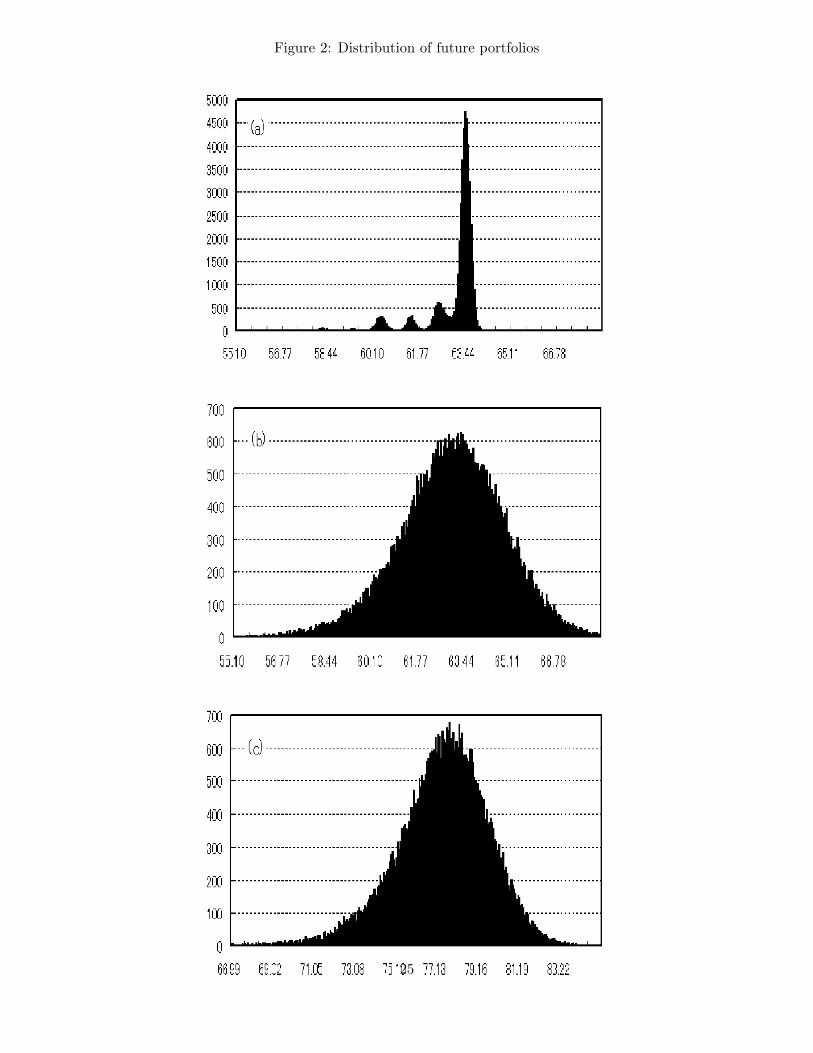
Figure 2: Distribution of future portfolios

25

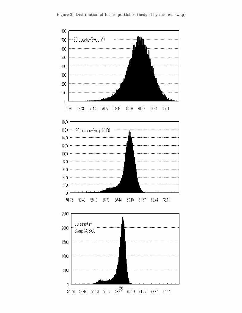
Figure 3: Distribution of future portfolios (hedged by interest swap)

26

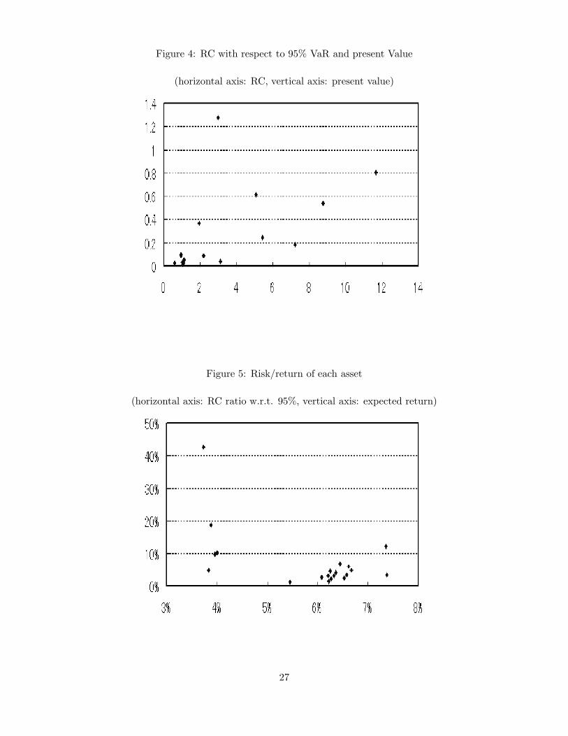
Figure 4: RC with respect to 95% VaR and present Value

(horizontal axis: RC, vertical axis: present value)

Figure 5: Risk/return of each asset

(horizontal axis: RC ratio w.r.t. 95%, vertical axis: expected return)

27

Figure 6: RC measure of each asset

(vertical axis: value of portfolio)

has some drawbacks (there is a possibility that the interest rate and hazard rate turn negative, or

that the relation between hazard rate and stocks is not fully expressed). However, there are many

great advantages: we can integratively evaluate the market risk and the credit risk in a natural

way, the method is simple and easy to use, the theoretical background is clear and consistent, and

so on. These advantages make up for the drawbacks to a satisfactory extent. This model relates

closely to the pricing model of default swaps proposed by Kijima [15] and in Kijima and Muromachi

[16], and we can directly apply this model to testing the hedging strategies of credit risk by credit

derivatives. Moreover, though omitted in this paper, it is possible to incorporate the effect of chain

default into this evaluation.

We have introduced an integrative evaluation model of market and credit risk. However, there

are many other important risks to be evaluated such as prepayment risks, liquidity risks, and so

on. The next task is the integration of other risks to the two already dealt with.

28

Endnotes

1 Refers to the risk-adjusted probability measures such as risk-neutral measure or forward-neutral measure. These

probability measures are used only to evaluate asset prices.

2 With Japan Financial Systems Rsearch Institute and Sumitomo Computer Systems Corporation, we are now jointly

developing a practical model based on the framework in this paper.

3 Kijima and Muromachi [17] set hazard rates as Ito processes with deterministic function parameters which are

constant in Jarrow and Turnbull [9]. Another difference is that hazard processes of firms are modeled in KM, while

forward rate processes of firms are modeled in JT.

4 Of course, we assume that all SDEs have a strong solution. For example, all parameters are assumed to satisfy

Lipschitz and growth conditions. We adopt a 1-factor model for simplicity, but it is fairly easy to extend to multi-

factor model.5 We omitted details, but this transformation is guaranteed by the Girsanov theorem, which is often used in the

pricing of derivatives. We implicitly assume that the sufficient condition for this theorem to holds such as (i) β0(t)

is Ft-measurable and continuous and (ii) the Novikov condition

E

[exp

1

2

∫ T∗

0

β20(s)ds

]< ∞

holds. Hereinafter, we omit this kind of statement unless it is needed.

6 j(t) in (10) is assumed to include the market price of risk corresponding to β0(t) in (8). Namely, adding j(t)

means that the Wiener process zj(t) under P is transformed to the processes zj(t) under P . In general, j(t) is

Ft-measurable as β0(t).

7 The following setting is an extention of Kijima and Muromachi [17]. Of course, all errors in this paper are the

responsibility of NLI Research Institute.

8 More pricisely, µs,j(t) and σs,j(t) in (11) are µs,j(Sj(t), r(t), hj(t), t) and σs,j(Sj(t), r(t), hj(t), t), respectively. (11)

implies that the expected instantaneous return is E[dSj(t)/Sj(t)]/dt = µs,j(t), where we have used hj(t) is the

intensity of τj .

9 In a similar manner, we can obtain the sufficent conditions for βn+j(t) to exist or the concrete expression of βn+j.

We can also derive the equation corresponding to rj(t) = r(t) + (1 − δj)hj(t) in Duffie and Singleton [5], where rj(t)

is an instantaneous spot rate of Firm j, and δj is the recovery rate of the discount bond issued by Firm j.

10 µV (t) and σV (t) depend on other variables as in the stock price processes.

11 Weibull distribution is a popular distribution in survival time analysis. Its hazard rate is given by h(t) = λγtγ−1.

λ and γ are called a scale parameter and a shape parameter, respectively. h(t) is increasing in t if γ > 1, constant if

γ = 1, and decreasing if 0 < γ < 1. In this case, we adopt a 3-parameter Weibull distribution with shift parameter

mj .

12 The recovery rates of bonds included in the portfolio can be set independently from the recovery rate of bonds

which defines the forward rates.

13 If the amount of each asset is fairly uniform and the portfolio is more diversified, these small peask overlaps and

the tail on the left side extends as a whole.

14 High face value is equivalent to high exposure because the loss amount is large when default occurs.

29

References

[1] Amin, K.I. and R.A. Jarrow (1991), “Pricing foreign currency options under stochastic interestrates,” Journal of International Money and Finance, 10, 310–329.

[2] Artzner, P. and F. Delbaen (1995), “Default risk insurance and incomplete markets,” Mathe-matical Finance, 5, 187–195.

[3] Credit Suisse Financial Products, (1997), CREDITRISK+.

[4] Duffie D. and M. Huang (1996), “Swap rates and credit quality,” Journal of Finance, 51,921–949.

[5] Duffie, D. and K. Singleton (1999), “Modeling term structures of defaultable bonds,” Reviewof Financial Studies, 12, 687–720.

[6] Fons, J.S. (1994), “Using default rates to model the term structure of credit risk” FinancialAnalysts Journal, September/October, 25–32.

[7] Hull, J. and A. White, (1990), “Pricing interest-rate-derivative securities,” Review of FinancialStudies, 3, 573–592.

[8] Inui, K. and M. Kijima (1998), “A Markovian framework in multi-factor Heath-Jarrow-Mortonmodels,” Journal of Financial and Quantitative Analysis, 33, 423–440.

[9] Jarrow, R.A. and S.M. Turnbull (1995), “Pricing derivatives on financial securities subject tocredit risk,” Journal of Finance, 50, 53–86.

[10] Jarrow, R.A. and S.M. Turnbull (1996), Derivative Securities, South-Western College Publish-ing.

[11] JPMorgan, (1997a), RiskMetricsTM Technical Document.

[12] JPMorgan, (1997b), CreditMetricsTM Technical Document.

[13] Kijima, M. (1998), “Monotonicities in a Markov chain model for valuing corporate bondssubject to credit risk,” Mathematical Finance, 8, 229–247.

[14] Kijima, M. (1999), “A Gaussian term structure model of credit risk spreads and valuation ofyield-spread options,” Working Paper, Tokyo Metropolitan University.

[15] Kijima, M. (2000), “Valuation of a credit swap of the basket type,” Review of DerivativesResearch, 4, 79–95.

[16] Kijima, M. and Y. Muromachi (2000a), “Credit events and the valuation of credit derivativesof basket type,” Review of Derivatives Research, 4, 53–77.

[17] Kijima, M. and Y. Muromachi (2000b), “Evaluation of credit risk of a portfolio with stochasticinterest rate and default processes,” Journal of Risk, accepted.

[18] Rockafellar, R. T. and S. Uryasev (2000), “Optimization of conditional value-at-risk,” Journalof Risk, 2, No3, 21–41.

[19] Tanaka, S. and Y. Muromachi (1999), “A new method for evaluating and managing the com-plex risks embedded in the life insurer’s balance sheet: basic ideas and preliminary results,”Joint Day Proceedings of the 30th International ASTIN Colloquium and the 9th InternationalAFIR Colloquium, Tokyo, 195–226.

30