an input-output approach in assessing the impact of...
TRANSCRIPT

1
AUA Working Paper Series No. [2010-1]
January 2010
An input-output approach in
assessing the impact of extensive
versus intensive farming systems
on rural development: the case of
Greece
Elias Giannakis
Department of Agricultural Economics & Rural Development
Agricultural University of Athens
Agricultural University of Athens ∙
Department of Agricultural Economics
& Rural Development ∙ http://www.aoa.aua.gr

2
An input-output approach in assessing the impact of extensive
versus intensive farming systems on rural development: the case
of Greece
Abstract
This paper analyses the role of the extensive versus the intensive farming systems
on rural development and specifically in a Greek rural area Trikala. The Generation
of Regional Input Output Tables (GRIT) technique is applied for the estimation of
the socio-economic impact of the farming systems through the estimation of an
input-output (I/O) table. This is followed by an agriculture-centred multiplier
analysis. The results suggest that intensive crops create stronger backward
linkages from extensive ones. Almost all farming systems appear to have rather
low Type 1 and Type 2 income and employment multipliers. Amongst them
extensive crops seem to have the greatest due to high direct income and
employment effects they create. Finally, the paper assesses the impact of the shift
of land resources from intensive to extensive farming systems, due to the Mid-term
Review of CAP, by exogenizing the output of the agricultural farming systems. The
results of the above analysis indicate a reduction in the sectoral output of the
region‟s economy.
Key words: intensive vs extensive farming systems; rural development; input-output analysis; CAP
JEL Classification: C67, O18, O13
1. Introduction
In the recent reform of CAP (2003/2004), the EU took a step towards maintaining
and improving the multifunctional role of agriculture. This refers mainly to the
introduction of “decoupling”, “modulation” and “cross-compliance”. In the same
period, environmental protection and land management has become a key policy
objective (Axis 2) of the EU rural development policy. These significant changes

3
have introduced reallocation of land resources from intensive to extensive farming
systems and have initiated restructuring in rural areas.
Under these circumstances, the analysis of the impact of extensive vs intensive
farming systems on the development of rural areas should identify:
a. the farming systems which create the strongest backward linkages with the
other sectors of the economy and contribute to the economic development of
the area; and
b. how farm land reallocation from intensive to extensive crops, due to CAP
reform, affects the total output of the regional economy.
In order to fulfill these objectives, this paper focuses on the application of the well-
established input-output technique with particular attention to the role of different
farming systems in rural development through final demand multiplier analysis.
Often however, agricultural policies or other external factors induce exogenous
changes in sectors‟ output which do not relate to final demand changes. In such
cases, as the change in the mix of farming systems described here, it is essential
to transfer the relevant exogenous changes on the sectors‟ output in order to
measure the impact on the rest of the economy.
This analysis is carried out for the Greek study area of Trikala, a NUTS III-level
area and “predominant rural” according to OECD classification (OECD, 1994).
Trikala depends heavily on agriculture as agricultural employment accounts to 30%
of total employment, while GDP in agriculture contributes to 15% of total GDP
formation.
2. Methodological aspects of the input-output analysis
2.1 Input-output multiplier analysis
Input-output analysis is a quantitative technique for studying the interdependence
of production sectors in an economy. An input-output table identifies the major
sectors in an economy and the financial flows between them over a stated time
period (usually a year). It indicates the sources of each sector‟s inputs, whether

4
purchased from other firms in the economy, imported or earned by labour
(household wages and salaries). It also provides a breakdown of each sector‟s
output, which can be sales to other sectors and to final demand (household
consumption, government consumption, capital formation and exports). The
interdependence between the individual sectors of the given economy is normally
described by a set of linear equations, representing fixed shares of input in the
production of each output. Thus, by disaggregating the total economy into a
number of interacting sectors, input-output analysis provides an effective tool for
sectoral and impact analysis.
Within a macroeconomic framework, input-output modeling creates a basis for the
evaluation of sectoral policies with respect to national or regional goals such as
GDP, employment and the balance of trade. Also, it provides more general
information compared to partial equilibrium models which concentrate on one
sector and more disaggregated information compared to purely macroeconomic
models.
An input-output model can be used for structural analysis, technical change
analysis and forecasting. However, the most popular application of the I-O
technique is impact analysis, where the model is used to estimate direct and
indirect effects on related sectors and on the whole economy resulting from
increased demand for the output of one or more sectors. These effects are
measured as changes in output, income and employment, and are reflected in
sectoral multipliers which express the ratio of total effect to the initial change in
demand.
For any one sector, a high level of intermediate inputs, ie., those purchased from
local firms, suggests strong linkages within economy and creates significant
indirect effects in the output of supplying sectors. These effects are quantified by
Type 1 output, income and employment multipliers.
1Direct and indirect effects
Type multiplierDirect effects

5
Further economic activity, stimulated by increased household spending is termed
the induce effect and is incorporated in the Type 2 multipliers:
,2
Direct indirect and induced effectsType multiplier
Direct effects
Both these multipliers have value greater than 1.0, with their magnitude depending
on the strength of the indirect and induced effects (Psaltopoulos, 1995).
The development of regional input-output models dates from the early 1950s. The
various approaches to constructing a regional input-output table can be broadly
categorized as „survey‟, „non-survey‟ and „hybrid‟ (Richardson 1972). The „survey‟
approach attempts to determine the regional input-output table by collecting
primary data through various survey methods. The advantage of this approach is
that it does not assume similarity between regional and national production
functions. On the other hand, the vast amount of data required, makes the survey
approach extremely expensive and time-consuming.
The „non-survey‟ approach involves the representation of the regional economy
through the modification of national technical coefficients. This stems from the fact
that a regional economy is normally less diverse and more import-dependent than
a national economy, because, besides receiving international imports, it also
imports goods and services from other regions (Round, 1972). A number of
methods have been developed, from the simple method of unadjusted national
coefficients to more sophisticated techniques. However, none of these „non-survey‟
methods provide satisfactory substitutes for the „survey‟ approach as the
constructed regional tables are not free from significant error (Richardson, 1972).
In response to this problem, a „hybrid‟ approach involves the application of „non-
survey‟ techniques to estimate an initial regional transactions matrix. Then, entries
in this matrix relating to key or problem sectors are replaced by survey-based
estimates. One of the most well-known hybrid techniques is GRIT (Generation of
Regional Input-Output Tables).

6
2.2 The GRIT approach
The GRIT technique was developed and originally applied for the estimation of
input-output tables for the regions of Queensland by Jensen et al (1979) and later
used by Johns and Leat (1987), Psaltopoulos and Thomson (1993), Tzouvelekas
and Mattas (1999) and Ciobanu et al. (2004). According to Jensen et al. (1979),
GRIT system was developed „…to provide an operational method, free from
significant error, for regional economic analysis‟. A mechanical procedure
(application of location quotients) is initially applied to adjust national tables. Then,
the analyst can determine the extent to which he/she „interferes‟ by the insertion of
„superior‟ data from survey or other sources. As a result, GRIT includes the
advantages of both „survey‟ and „non-survey‟ techniques.
In summary, the GRIT method estimates the flows (million euro) of the regional
Intermediate Demand and Primary Inputs quadrants by applying regional-to-
national employment ratios and Cross-Ιndustry Location Quotients to the
corresponding flows of the national quadrants. The regional Final Demand
quadrants are estimated by multiplying the national quadrant by the regional-to-
national employment ratio for each sector. The Consumption column of the Final
Demand quadrant is further adjusted through the use of location quotients.
Regional Exports for each sector are calculated as a residual, ie., the difference
between regional output and the sum of intermediate output, regional household
consumption and other final demand.
At this point, the full form of the generated regional table may contain a number of
sectors which are relatively insignificant within the regional economy. A suitable
aggregation scheme to reduce the sectoral detail may be determined by the
objectives of the study. However, the application of location quotients must take
place before sectoral aggregation, because, as employment data become more
aggregated, quotients tend to unity. As a result, regional imports will be
underestimated and regional multipliers overestimated. After aggregation, superior
data can be inserted, but should be fully compatible with the definition of the
aggregate sectors.

7
2.3 Application of input-output analysis in the evaluation of agriculture‟s role in the
economy
A number of studies, employing input-output analysis, appeared in the literature
dealing with the estimation of agriculture‟s economic impacts on national or
regional level. Agriculture plays an important role in the economy and especially in
the economy of rural areas as it procures production inputs from, and produces
inputs to, other sectors. Input-output models provide an appropriate framework for
tracing these linkages in the economy. Henry and Schulder (1985) by measuring
the backward and forward linkages of food and fiber sector in USA, stress the
importance of agriculture. They state that the impact of agriculture in the whole
economy is influenced not only by the magnitude of the linkages and the
interdependence among the sectors of the economy, but also by the structure of
the particular economy and the relative shares of the raw and processed food
sectors. Tzouvelekas and Mattas (1999) examine the role of agro-food sector in
the local economy of the Greek island Crete. Cummings et al (2000) investigate
the role of farming sector in the local economy of Ontario region and evaluate the
direct and indirect effects of agriculture to the rest sectors. The collective volume of
Midmore and Harrison-Mayfield (1996), presents a number of studies examining
the role of agriculture in an economy by utilizing I-O analysis. Sharma et al (1999)
investigate the role of agriculture to the economy of Hawaii. Hamilton et al. (1991)
and Baumol and Wolff (1994), both in their studies stress the significance of
indirect effects of agriculture in the economy. However, very little analysis has
actually taken place about the impact of disaggregated farming systems on the
development of rural areas.
2.4 Theoretical aspects of exogenizing sectoral outputs
Input-output analysis implicitly assumes that all endogenous sectors can produce
any level of output required to meet final demands. Given this assumption,
changes in the elements of final demand can be introduced to the input-output
model, and through the calculation of final demand input-output multipliers as
presented above, total effects on each sector can be measured. Often however,
policies or uncontrollable factors induce exogenous changes in total outputs of
sectors and commodities. Since what is exogenously altered is the output of
sectors or commodities not belonging to the exogenous final demand, the use of

8
final demand multipliers induces bias and inflates the results (Papadas and Dahl,
1999).
Attempts to resolve the problem include the development of an iterative linear
programming solution applied to the input-output model as one method of handling
exogenous constraints on sectoral outputs, which are predetermined rather than
simultaneously determined by final and intermediate demand (Petkovich and
Ching, 1978). Final demand changes are then accommodated subject to these
constraints. This scenario is a special case of the more general one in which the
output of a given sector or commodity is restricted to some predetermined level.
Such cases are output‟s reduction because of policy changes (Bromley et al.,
1968) or cases where production is increased because of irrigation and generally
all those cases where the objective is to determine the impact, not of changes in
final demand, but changes in total output. To accommodate this more general
scenario, Johnson and Kulshreshtha (1982) propose a procedure within input-
output framework which leads to a new set of multipliers which Papadas and Dahl
(1999) call “supply-driven” for obvious reasons.
The usefuleness of these supply-driven multipliers according to Papadas and Dahl
(1999) is not limited to impact analysis of specific exogenous changes in total
outputs but they can also be used to assess the output effects of economic
phenomena of wider economic processes by translating accurately these
phenomena into output changes. In Henry et al. (1986) for example, changes in
farm size and type distributions are translated into exogenous output changes, and
such multipliers are used to evaluate the implications of structural changes in the
farm sector for the non-farm economy.
The procedure of Johnson and Kulshreshtha (1982) to exogenise a given set of
outputs is described here. The basic equation of input-output analysis is:
X AX F (1)
Using subscript 1 to denote the sectors whose outputs are to be exogenised and
subscript 2 for the rest, with matrix partitioning (1) can become:

9
1 11 12 1 1
2 21 22 2 2
X M M X F
X M M X F
(2)
which represents a system of two matrix equations. The unknowns now are X2 and
F1 while X1 and F2 are exogenously determined. Solving the second equation
yields:
1
2 22 21 1 2( ) ( )X I M M X F (3)
Given the levels of X1 and F2 (or their change), the level of X2 (or its change) can
be estimated from (3). Inserting this value in the first equation of the system gives
the new value of F1 or its change:
1 11 1 12 2( )F I M X M X (4)
If the interest is only in the impact of exogenous changes in outputs, on other
outputs, one can assume the change in F2 to be zero and the suggested multipliers
matrix from (3) is
1
22 21( )I M M (5)
If k sectors are exogenised, the matrix is of dimension (m-k, k) and the ijth element
shows the change in sector i‟s output due to a unitary change in sector j‟s output.
3. The socio-economic profile of the study area Trikala
The prefecture of Trikala belongs to the region of Thessaly and is located in the
central part of Greece. Its land area amounts to 3.384 km2 (2,5% of land of
Greece) of which 83% is mountainous and semi-mountainous and only 18% is
level area. Its population, in 2001, amounted to 138.047 people, with very low
density (40,8 persons/km2), much lower compared to the national average (83,1
persons/km2). The population in Trikala was declining following the general trend in

10
Greek rural areas. However during the 1990s, population remained stable,
compared to the overall depopulation trend in mountainous areas of Greece.
The primary sector has traditionally been the main productive sector in the area. In
1971, almost two thirds (66%) of total employment were in agricultural activities.
However, in the last few decades the continuing exodus from agriculture was
followed by the expansion of services (50% of total employment in 2001), while the
relevant share of the secondary sector has remained stable (around 20%) since
1981. Albeit, in relation to the national average (14,7%), the prefecture still remains
dependent on agriculture, as a significant part of the labour force is still occupied in
agricultural activities (30% in 2001).
During the period 2000-2006, GDP (current prices) in Trikala increased with an
annual growth rate of 6,7% compared to 7,7% in Greece. In a similar manner, GDP
per capita at the same period increased by an annual growth rate of 7%, compared
to 7,4% at the national level. As a result, in 2006 GDP per capita in Trikala
represented 60% of the national average (Giannakis, 2006). In terms of the
sectoral shares of GDP, it is important to note the high contribution of services to
the formation of GDP in Trikala (67% in 2001).
The number of farms in Trikala amounts to 15.619 (Agricultural Census 2000) with
an average size quite low (3,9 ha vs 4,4 ha nationally). Agricultural utilized area is
about 60.000 hectares, of which 70% is irrigated. Predominant cultivated crops are
mainly arable crops, such as wheat, maize, cotton, barley, fodder crops etc.
Livestock farming is mainly based on extensive sheep, goat and cattle grazing
systems and consists a very important component of primary economic activity in
the mountainous areas of Trikala, as it concentrates in the mountainous part of the
prefecture.
The farming systems in Trikala region are quite diverse. Based on the FADN data,
four farming systems seem to prevail: (a) extensive crop production of cereals, (b)
extensive livestock farming and sheep grazing, (c) intensive farming of irrigated
crops of cotton, maize, sugarbeets etc and (d) other agricultural system (residual)
including land under tree cultivation and other minor crops.

11
4. Analysis and Results
4.1 The construction of the Trikala input-output table
The basis of the analysis is the 2000 Greek symmetric „commodity-by-commodity‟
input-output table, updated to 2004 by the application of the RAS method (O‟
Connor and Henry, 1975). The year 2004 was chosen as the base year since it is
the first year after the implementation of CAP reform (2003-2004). The initial
scheme of 59 sectors of economic activity ended to 18 after the aggregation.
The next step was the construction of the regional input-output table for Trikala
region using the GRIT technique described above. This method was chosen
because the cost of using a full survey-based method to generate the regional
tables was prohibitive and regional I-O tables constructed via non-survey
techniques are not sufficiently accurate (Richardson, 1972). Furthermore, as noted
by Johns and Leat (1987), GRIT is particularly suitable for smaller regions, as it
allows the more accurate estimation of the (expectedly) smaller multipliers that
characterize small regional economies.
According to Jensen et al. (1979), „superior‟ data can be selected according to
objectives and resources and can be confined to sectors of particular interest.
Czamanski and Malizia (1969) suggest that superior data should be obtained for
sectors in which the economy under study is specialized. In order to investigate in
further detail the relationships between local economic sectors and the rest of the
rural economy, primary data available from a survey of enterprises of the most
important sectors of the study area was utilized. The selection of sampled sectors
was based on the following two criteria: (a) significance of sectors in regional
economy and (b) existence of strong intersectoral linkages with the products of the
agricultural sector. Along those lines, the survey was carried out to the following
sectors: agriculture, food manufacturing, trade and tourism. The final I/O table
constructed consists of 21 sectors of economic activity: 17 non-agricultural and 4
agricultural as the agricultural sector is disaggregated into four farming systems:
extensive arable crops, extensive livestock, intensive arable crops and other
agricultural system.

12
4.2 Output multipliers
Based on the constructed I/O table for Trikala, Table 1 indicates the Type 1 output
multipliers which express the regional significance of the backward linkages of
each sector. The multiplier for the farming system of intensive crops is amongst the
highest (3rd in rank), while for the farming system extensive arable is relatively low,
indicating weak linkages with other sectors. So, a unit increase in the final demand
for the products of the intensive crops farming system (i.e., exports, consumption
or investments) will increase the total (direct and indirect) output in the region of
Trikala by 1,653 units. The highest backward linkages amongst the non-agricultural
sectors are created by the products of the sector of trade (1,78) followed by the
sector of metal products (1,66) and tourism (1,573).
The largest induced effects (Type 2 output multipliers) tend to be in the farming
systems of other agr system (3,251 – 3rd in rank) and extensive livestock (2,679 –
4rth in rank). This is because wages and salaries represent a large proportion of
their total inputs. Multiplier for the farming system of extensive arable is not
amongst the highest, albeit not low. The highest induced effects amongst the non-
agricultural sectors are created by the products of the sectors of public
administration (3,561), education (3,538) and other services (2,643). The large
proportion of inputs accounted for by wages and salaries in the sectors of
agriculture and services contributes to a significant rise in regional incomes and
household spending as output increases.
Table 1. Output multipliers for prefecture Trikala (2004)
Sectors of economic activity Type 1 Rank Type 2 Rank
Extensive arable 1,444 10 2,163 13
Extensive livestock 1,548 6 2,679 4
Intensive arable 1,653 3 2,566 7
Other agr system 1,634 4 3,251 3
Mining 1,157 20 1,646 20
Food manufacture 1,298 16 1,683 19
Textile 1,524 7 2,181 11
Wood and paper 1,457 9 2,181 12
Chemical and plastic products 1,484 8 1,913 18

13
Non metal products 1,430 12 2,252 10
Metal products 1,660 2 2,288 9
Machinery and equipment 1,197 19 1,550 21
Electricity, gas and water 1,204 18 1,941 16
Construction 1,433 11 2,113 14
Trade 1,780 1 2,540 8
Tourism 1,573 5 2,097 15
Transportation 1,396 13 2,587 6
Banking-Financing 1,360 14 1,932 17
Public administration 1,344 15 3,561 1
Education 1,062 21 3,538 2
Other services 1,257 17 2,643 5
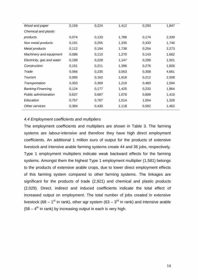
4.3 Income coefficients and multipliers
Table 2 shows income coefficients and multipliers. Income coefficients indicate the
total increase in incomes generated by a unit increase in the output of the products
of a particular sector. Direct income coefficients (DICs) for other agr system and
extensive livestock are amongst the highest, while capital-intensive sectors such
as trade, chemical and plastic products and food manufacture have low
coefficients. Type 1 income multipliers for the farming systems are rather low with
the highest appearing to the farming system of extensive arable (1,599 – 5th in
rank) and intensive arable (1,485 – 7th in rank). The sectors of trade (3,563) and
tourism (1,918) have the largest income multipliers amongst the non-agricultural
sectors. The Type 2 multipliers follow the same pattern as the Type 1 multipliers.
Table 2. Income coefficients & multipliers for prefecture Trikala (2004)
Sectors of economic
activity
Direct
Income
Coefficient
Direct & Indirect
Income
Coefficient
Type 1
Income
Multiplier
Direct, Indirect
& Induced
Income
Coefficient
Type 2
Income
Multiplier
Extensive arable 0,139 0,223 1,599 0,291 2,092
Extensive livestock 0,265 0,351 1,324 0,459 1,732
Intensive arable 0,191 0,283 1,485 0,370 1,943
Other agr system 0,400 0,501 1,254 0,656 1,640
Mining 0,131 0,152 1,161 0,198 1,518
Food manufacture 0,085 0,119 1,400 0,156 1,831
Textile 0,133 0,204 1,529 0,266 2,000
14
Wood and paper 0,159 0,224 1,412 0,293 1,847
Chemical and plastic
products 0,074 0,133 1,788 0,174 2,339
Non metal products 0,191 0,255 1,335 0,333 1,746
Metal products 0,112 0,194 1,738 0,254 2,273
Machinery and equipment 0,086 0,110 1,270 0,143 1,662
Electricity, gas and water 0,199 0,228 1,147 0,299 1,501
Construction 0,151 0,211 1,396 0,276 1,826
Trade 0,066 0,235 3,563 0,308 4,661
Tourism 0,085 0,162 1,918 0,212 2,508
Transportation 0,303 0,369 1,219 0,483 1,594
Banking-Financing 0,124 0,177 1,425 0,232 1,864
Public administration 0,637 0,687 1,078 0,899 1,410
Education 0,757 0,767 1,014 1,004 1,326
Other services 0,384 0,430 1,118 0,562 1,462
4.4 Employment coefficients and multipliers
The employment coefficients and multipliers are shown in Table 3. The farming
systems are labour-intensive and therefore they have high direct employment
coefficients. An additional 1 million euro of output for the products of extensive
livestock and intensive arable farming systems create 44 and 36 jobs, respectively.
Type 1 employment multipliers indicate weak backward effects for the farming
systems. Amongst them the highest Type 1 employment multiplier (1,581) belongs
to the products of extensive arable crops, due to lower direct employment effects
of this farming system compared to other farming systems. The linkages are
significant for the products of trade (2,921) and chemical and plastic products
(2,029). Direct, indirect and induced coefficients indicate the total effect of
increased output on employment. The total number of jobs created in extensive
livestock (68 – 1st in rank), other agr system (63 – 3rd in rank) and intensive arable
(58 – 4th in rank) by increasing output in each is very high.

15
Table 3. Employment coefficients & multipliers for prefecture Trikala (2004)
Sectors of economic
activity
Direct
Employment
Coefficient
Direct &
Indirect
Employment
Coefficient
Type 1
Employment
Multiplier
Direct, Indirect
& Induced
Employment
Coefficient
Type 2
Employment
Coefficient
Extensive arable 22 35 1.581 42 1.899
Extensive livestock 44 57 1.306 68 1.559
Intensive arable 36 49 1.368 58 1.619
Other agr system 34 47 1.361 63 1.821
Mining 4 5 1.459 10 2.776
Food manufacture 6 9 1.627 13 2.306
Textile 10 16 1.582 23 2.201
Wood and paper 15 22 1.450 29 1.921
Chemical and plastic
products 3 7 2.029 11 3.238
Non metal products 9 14 1.530 22 2.406
Metal products 10 17 1.741 23 2.385
Machinery and
equipment 6 8 1.361 11 1.954
Electricity, gas and
water 6 8 1.363 15 2.604
Construction 18 24 1.287 30 1.648
Trade 13 38 2.921 45 3.497
Tourism 14 22 1.610 27 1.982
Transportation 20 26 1.283 38 1.855
Banking-Financing 10 15 1.451 20 1.997
Public administration 26 30 1.156 52 1.984
Education 38 39 1.022 63 1.662
Other services 27 30 1.135 44 1.646
4.5 Farming systems „supply-driven‟ multipliers
To assess the impact of the farming systems on the local economy from the supply
side, it is necessary to exogenize the output of the farming systems based on the
methodology described above in paragraph 2.4. In Table 4, „supply-driven‟
multipliers of each farming system for the rest sectors of economy are presented.
Each element shows the output change of the ith sector due to the exogenous
change of the output of the corresponding farming system. The sum of the
column‟s elements shows the total impact of the exogenous change of the output

16
of the different farming systems by one unit on the local economy‟s output. In other
words, if the output of intensive arable system increases by 1 million euro, the
output of the other sectors of local economy will increase by 0,5381 million euro.
Extensive arable farming system creates a lower impact on the local economy
(0,4256) compared to the intensive one (0,5381). It is noted that the other agr
system appears to have a rather high multiplier (0,5568).
Table 4. ‘Supply-driven’ multipliers of different farming systems to the local
economy
Sectors of economic
activity
Extensive
arable
Extensive
livestock
Intensive
arable
Other agr
system
Extensive arable - 0,0541 0,0000 0,0108
Extensive livestock 0,1935 - 0,0002 0,0839
Intensive arable 0,0373 0,1601 - 0,0383
Other agr system 0,0087 0,0107 0,0003 -
Mining 0,0012 0,0019 0,0073 0,0039
Food manufacture 0,0002 0,0002 0,0045 0,0003
Textile 0,0001 0,0001 0,0023 0,0002
Wood and paper 0,0014 0,0017 0,0135 0,0029
Chemical and plastic products 0,0028 0,0032 0,0115 0,0063
Non metal products 0,0001 0,0001 0,0289 0,0002
Metal products 0,0003 0,0004 0,0262 0,0008
Machinery and equipment 0,0021 0,0025 0,0138 0,0047
Electricity, gas and water 0,0200 0,0364 0,0380 0,0770
Construction 0,0006 0,0007 0,0018 0,0019
Trade 0,1406 0,1728 0,3543 0,2755
Tourism 0,0002 0,0002 0,0005 0,0005
Transportation 0,0122 0,0069 0,0239 0,0238
Banking-Financing 0,0034 0,0020 0,0105 0,0236
Public administration 0,0000 0,0000 0,0000 0,0000
Education 0,0000 0,0000 0,0000 0,0000
Other services 0,0010 0,0010 0,0006 0,0020
Total 0,4256 0,4550 0,5381 0,5568
4.6 Impact assessment of the land reallocation due to the CAP Reform (2003-
2004)
The implementation of the Mid-term Reform of CAP has resulted in significant
changes in the agricultural sector of the prefecture Trikala as well as at national

17
level. The overwhelming bulk of production-linked and hence production-
incentivising subsidies has been replaced by the Single Farm Payment (SFP)
which does not require specific farm output or even specific farm input use.
Specifically, in Trikala, upon the initiation of the CAP reform and between 2004-
2007, 3.850 hectares were moved from intensive arable to extensive arable crops
representing 12% of the intensive cropping land. This reallocation of land resulted
in changes in the value of output of extensive arable by 7.104.471 euro which
accounts for 2% of the total agricultural gross output. Replacing in equation (3) ΔΧ1
= 7.104.471 euro, total output generated in the economy is about ΔΧ2 = 3.023.663
euro. On the other hand, the output of the intensive arable farming system is
decreased by 15.135.350 euro and as a result the total output of the local economy
is reduced by 8.144.332 euro. In total, the net output of regional economy is
reduced by 5.120.669 euro.
However, in this point it must be mentioned that agriculture beyond its primary
function of producing food and fiber commodities, produces jointly a wide range of
non-commodity outputs, some of which exhibit the characteristics of public goods
or externalities (OECD, 2001). So, changes in land use and farming systems alter
not only the levels of commodity outputs as calculated above but also the mix of
non-commodities generated jointly during the production process.
It is widely acknowledged that low-input farming systems are more in „harmony‟
with „natural‟ ecological processes, contributing positively to the provision of such
„non-market‟ functions as biodiversity, landscape, water and air quality (Bignal,
1998; Phillips, 1998; Smeding and Joenje, 1999; Kolpin, 1997). In contrast, the
intensification of agriculture has detrimental consequences for biodiversity (Donald
et al 2001; McLaughlin 1995; Robinson & Sutherland 2002), water quality
(Sutherland 2002) etc. putting at risk the resilience of ecosystems (Knickel, 1990).
Furthermore, low-input agricultural activities provide important amenities in rural
areas. As society places an increasing value on the preservation of the
environment, the semi-natural habitats and the scenic features of cultivated
landscapes, the aesthetic, ecological, cultural and historic aspects of such rural
landscapes contribute positively to regional attractiveness for tourism sector as
well as the quality of life of regional citizens. However, it is beyond the scope of

18
this paper to estimate the gains for the local economy of the non-commodities
produced by the extensive agricultural systems and which tend to compensate for
the net output losses.
5. Conclusions
Input-output multiplier analysis shows that the farming system of intensive crops
creates the strongest backward linkages with the other sectors of economy.
Income and employment multipliers are rather low for almost all the farming
systems with the system of extensive crops having the greatest one due to high
direct income and employment effects they create. Amongst non-agricultural
sectors, products of trade and tourism seem to create the greatest backward
linkages with the rest economy. The Mid-term Reform of CAP (2003/2004) and the
implementation of the Single Farm Payment regime have initiated changes in rural
areas and have introduced reallocation of land resources from intensive to
extensive farming systems. From the above analysis it seems that the net output
generated from the land reallocation is negative for the rural economy. However,
the process of land reallocation seems to be at initial stage and it is expected to go
on. Considering also that, European policy initiatives aiming at strengthening the
viability of rural areas have as central point the multifunctional role of agriculture
and stress the importance of safeguarding the provision of agri-environmental
goods, it is essential to take into consideration that this land reallocation enhance
the generation of such positive externalities from agriculture and must be further
investigated in future research.
Acknowledgements
The author would like to thank his Ph.D advisor Prof. S. Efstratoglou, for her
guidance and constructive comments, T. Kampas and C. T. Papadas, Assistant
Professors and D. Psaltopoulos, Associate Professor, for their useful comments.

19
References
Bignal, E.M., 1998. Using an ecological understanding of farmland to reconcile
nature conservation requirements, EU agriculture policy and world trade
agreements. Journal of Applied Ecology 35 (6), pp. 949-954.
Baumol, J. and Wolff, N., 1994. A key role of Input-Output analysis in policy
design. Regional Science and Urban Economics 24, pp. 93-114.
Bromley, D. W., Blanch, G. E. and Stoevener, H. H., 1968. “Effects of Selected
Changes in Federal Land Use on a Rural Economy”, Station Bulletin #604,
Agricultural Experiment Station, Oregon State University, March, 1968.
Ciobanu, C., Mattas, K. and Psaltopoulos, D., 2004. Structural Changes in Less
Developed Areas: An Input–Output Framework. Regional Studies 38 (6), pp.
603–614.
Czamanski, S. and Malizia, E.E., 1969. Applicability and limitations in the use of
national input-output tables for regional studies. Regional Science Association
Papers and Proceedings 23.
Cummings, H., Murray, D., Morris, K., Keddie, P., Xu, W., Deschamps, V., 2000.
“The Economic Impacts of Agriculture on the Economy of Frontenac, Lennox &
Addington and the United Coumties of Leeds and Grenville”. Socio-Economic
Profile and Agriculture-Related Business Survey, Final Report, Ministry of
Agriculture, Food and Rural Affairs.
Donald, P.F., Green, R.E., Heath, M.F., 2001. Agricultural intensification and the
collapse of Europe‟s farmland bird populations. Proc. R. Soc. London B 268,
pp. 25–29.
Hamilton R., Whittlesey K. Robinson H. and Ellis J., 1991. Economic-impacts,
value added and benefits in regional project analysis. American Journal of
Agricultural Economics 73, pp. 334-344.
Giannakis, E., 2006. An input-output analysis of inter-industry linkages and the role
of agricultural sector in the economic development of Trikala region.
Unpublished Master Thesis, Agricultural University of Athens, Athens, 2006.
Henry, M. and Schluter, G., 1985. Measuring backward and forward linkages in the
US food and fiber system. Agricultural Economics Research 37 (4), pp. 33-39.

20
Henry, M., Somwaru, A., Schluter, G. And Edmonson, W., 1986. Some Effects on
Farm Size on the Non-Farm Economy. North Central Journal of Agricultural
Economics 7, pp. 187-198.
Jensen, R.C., Mandeville, T.D. and Karunaratne, N.D., 1979. Regional Economic
Planning. Croom Helm, London.
Johns, P. M. and Leat, P. M. K., 1987. The application of modified GRIT input-
output procedures to rural development analysis in Grampian Region. Journal
of Agricultural Economics 38, pp. 242-256.
Johnson, T. G. and Kulshreshtah, S. N., 1982. Exogenising Agriculture in an Input-
Output Model to Estimate Relative Impacts of Different Farm Types. Western
Journal of Agricultural Economics 9 (1), pp. 1-11.
Knickel, K., 1990. Agricultural structural change: Impact on the rural environment.
Journal of Rural Studies 6 (4), pp. 383-393.
Kolpin, D.W., 1997. Agricultural Chemicals in Groundwater of the Midwestern
United States: Relations to Land Use. Journal of Environmental Quality 26 (4),
pp. 1025-1037.
McLaughlin, A. and Mineau, P., 1995. The impact of agricultural practices on
biodiversity. Agriculture Ecosystems and Environment 55, pp. 201-212.
Μidmore, P. and Harrison-Mayfield, L., 1996. Rural Economic Modelling. An Input-
Output Approach. Wallingford: CAB International.
O‟Connor, R. and Henry. E.W., 1975 Input-Output Analysis and its Applications.
Griffin, London.
OECD, 1994. Creating Rural Indicators for shaping territorial policy. Paris, OECD.
OECD, 2001. Multifunctionality: Towards and Analytical Framework. Paris, OECD.
National Statistical Service of Greece, Census of Agriculture 1999/2000, Athens,
Greece.
Papadas, C.T. and Dahl, D.C., 1999. Supply-Driven Input-Output Multipliers,
Journal of Agricultural Economics 50 (2), pp. 269-285.
Petkovich, M. D. and Ching, C. T. K., 1978. Modifying a One Region Leontief
Input-Output Model to Show Sector Capacity Constraints. Western Journal of
Agricultural Economics 3, pp. 173-179.
Phillips, A., 1998. The Nature of Cultural Landscapes - a nature conservation
perspective. Landscape Research 23 (1), pp. 21-38.

21
Psaltopoulos, D. and Thomson, K. J., 1993. Input-output evaluation of rural
development: a forestry-centred application. Journal of Rural Studies 9, pp.
351-358.
Psaltopoulos, D., 1995. Input-Output Analysis of Scottish Forestry Strategies.
Unpublished Doctoral Thesis, University of Aberdeen, Aberdeen, 1995.
Richardson, H., 1972. Input-Output and Regional Economics. Weidenfeld and
Nicolson, London.
Robinson, R.A. & Sutherland, W.J., 2002. Changes in arable farming and
biodiversity in Great Britain. Journal of Applied Ecology 39, pp. 157–176.
Round, J. I., 1972. Regional input-output models in the UK: a re-appraisal of some
techniques. Regional Studies 6, pp. 1-9.
Sharma, K., Leung, P. and Nakamoto, S., 1999. Accounting for the linkages of
agriculture in Hawaii‟s economy with an input-output model: A final demand-
based approach. The Annals of Regional Science 33, pp. 123-140.
Smeding, F.W. and Joenje, W., 1999. Farm-nature Plan: landscape ecology based
farm planning. Landscape and Urban Planning 46 (1-3), pp. 109-115.
Sutherland, W.J., 2002. Restoring a sustainable countryside. Trends in Ecology
and Evolution 17, pp. 148–150.
Tzouvelekas, V. and Mattas, K., 1999. Tourism and agro-food as a growth stimulus
to a rural economy: the Mediterranean island of Crete. Journal of Applied Input-
Output Analysis 5, pp. 69-81.