An In-Depth Look at the Information Ratio

by

Sharon L. Blatt

A Thesis

Submitted to the Faculty

of the

WORCESTER POLYTECHNIC INSTITUTE

In partial fulfillment of the requirements for the

Degree of Master of Science

in

Mathematical Science

August 2004

APPROVED:

Professor Arthur C. Heinricher, Thesis Advisor

Professor Bogdan Vernescu, Head, Mathematical Sciences Department

Abstract

The information ratio is a very controversial topic in the business world. Some portfolio

managers put a lot of weight behind this risk-analysis measurement while others believe

that this financial statistic can be easily manipulated and thus shouldn’t be trusted.

In this paper, an attempt will be made to show both sides of this issue by defining the

information ratio, applying this definition to real world situations, explaining some of

the negative impacts on the information ratio, comparing this ratio to other statistical

measures, and showing some ways to improve a portfolio manager’s information ratio.

ii

Acknowledgments

I would like to thank the faculty and students of the Mathematics Department for

their help and support during my tenure here at WPI. I would especially like to thank

Professor Heinricher for his patience and guidance in helping me with this project.

I would also like to thank my colleagues at Mechanics Co/operative Bank for al-

lowing me to have a more flexible schedule in order to finish this degree. Most of all

I want to thank my family and friends who have always supported me in everything I

do. And last, but not least, I would like to thank my boyfriend, Alan, for being there

for me and encouraging me when times got rough.

iii

Contents

1 Introduction 1

2 Background 3

2.1 Modern Portfolio Theory . . . . . . . . . . . . . . . . . . . . . . . . . . 4

3 Definitions of the Information Ratio 6

3.1 The First Definition . . . . . . . . . . . . . . . . . . . . . . . . . . . . . 7

3.2 The Second Definition . . . . . . . . . . . . . . . . . . . . . . . . . . . 8

3.3 The Third Definition . . . . . . . . . . . . . . . . . . . . . . . . . . . . 9

3.4 A “Good” Information Ratio . . . . . . . . . . . . . . . . . . . . . . . . 10

4 Applying the Definition 12

4.1 Opportunities Available . . . . . . . . . . . . . . . . . . . . . . . . . . 12

4.2 Value Added . . . . . . . . . . . . . . . . . . . . . . . . . . . . . . . . . 12

5 Negative Impacts on the Information Ratio 15

5.1 Negative Excess Returns . . . . . . . . . . . . . . . . . . . . . . . . . . 15

5.2 Transaction Costs . . . . . . . . . . . . . . . . . . . . . . . . . . . . . . 17

6 Comparison to Other Ratios 19

6.1 IR vs. t-statistic . . . . . . . . . . . . . . . . . . . . . . . . . . . . . . . 19

6.2 IR vs. Sharpe Ratio . . . . . . . . . . . . . . . . . . . . . . . . . . . . 20

7 IR Improvement Techniques 21

8 Conclusion 23

A Appendix: Stock Summaries 24

B Appendix: Tables 30

C Appendix: Figures 35

iv

D References 41

v

List of Tables

Table 1 . . . . . . . . . . . . . . . . . . . . . . . . . . . . . . . . . . . . . . . . . . . . . . . . . . . . . . . . . . . . . . . . . . . . . . . . 6

Table 2 . . . . . . . . . . . . . . . . . . . . . . . . . . . . . . . . . . . . . . . . . . . . . . . . . . . . . . . . . . . . . . . . . . . . . . . 10

Table 3 . . . . . . . . . . . . . . . . . . . . . . . . . . . . . . . . . . . . . . . . . . . . . . . . . . . . . . . . . . . . . . . . . . . . . . . 13

Table 4 . . . . . . . . . . . . . . . . . . . . . . . . . . . . . . . . . . . . . . . . . . . . . . . . . . . . . . . . . . . . . . . . . . . . . . . 31

Table 5 . . . . . . . . . . . . . . . . . . . . . . . . . . . . . . . . . . . . . . . . . . . . . . . . . . . . . . . . . . . . . . . . . . . . . . . 32

Table 6 . . . . . . . . . . . . . . . . . . . . . . . . . . . . . . . . . . . . . . . . . . . . . . . . . . . . . . . . . . . . . . . . . . . . . . . 33

Table 7 . . . . . . . . . . . . . . . . . . . . . . . . . . . . . . . . . . . . . . . . . . . . . . . . . . . . . . . . . . . . . . . . . . . . . . . 34

Table 8 . . . . . . . . . . . . . . . . . . . . . . . . . . . . . . . . . . . . . . . . . . . . . . . . . . . . . . . . . . . . . . . . . . . . . . . 18

List of Figures

Figure 1 . . . . . . . . . . . . . . . . . . . . . . . . . . . . . . . . . . . . . . . . . . . . . . . . . . . . . . . . . . . . . . . . . . . . . . 35

Figure 2 . . . . . . . . . . . . . . . . . . . . . . . . . . . . . . . . . . . . . . . . . . . . . . . . . . . . . . . . . . . . . . . . . . . . . . 36

Figure 3 . . . . . . . . . . . . . . . . . . . . . . . . . . . . . . . . . . . . . . . . . . . . . . . . . . . . . . . . . . . . . . . . . . . . . . 37

Figure 4 . . . . . . . . . . . . . . . . . . . . . . . . . . . . . . . . . . . . . . . . . . . . . . . . . . . . . . . . . . . . . . . . . . . . . . 38

Figure 5 . . . . . . . . . . . . . . . . . . . . . . . . . . . . . . . . . . . . . . . . . . . . . . . . . . . . . . . . . . . . . . . . . . . . . . 39

Figure 6 . . . . . . . . . . . . . . . . . . . . . . . . . . . . . . . . . . . . . . . . . . . . . . . . . . . . . . . . . . . . . . . . . . . . . . 40

vi

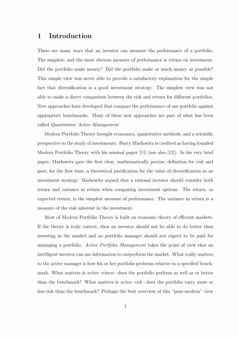
1 Introduction

There are many ways that an investor can measure the performance of a portfolio.

The simplest, and the most obvious measure of performance is return on investment.

Did the portfolio make money? Did the portfolio make as much money as possible?

This simple view was never able to provide a satisfactory explanation for the simple

fact that diversification is a good investment strategy. The simplest view was not

able to make a direct comparison between the risk and return for different portfolios.

New approaches have developed that compare the performance of one portfolio against

appropriate benchmarks. Many of these new approaches are part of what has been

called Quantitative Active Management.

Modern Portfolio Theory brought economics, quantitative methods, and a scientific

perspective to the study of investments. Harry Markowitz is credited as having founded

Modern Portfolio Theory with his seminal paper [11] (see also [12]). In his very brief

paper, Markowitz gave the first clear, mathematically precise, definition for risk and

gave, for the first time, a theoretical justification for the value of diversification as an

investment strategy. Markowitz argued that a rational investor should consider both

return and variance in return when comparing investment options. The return, or

expected return, is the simplest measure of performance. The variance in return is a

measure of the risk inherent in the investment.

Most of Modern Portfolio Theory is built on economic theory of efficient markets.

If the theory is truly correct, then an investor should not be able to do better than

investing in the market and no portfolio manager should not expect to be paid for

managing a portfolio. Active Portfolio Management takes the point of view that an

intelligent investor can use information to outperform the market. What really matters

to the active manager is how his or her portfolio performs relative to a specified bench-

mark. What matters is active return—does the portfolio perform as well as or better

than the benchmark? What matters is active risk—does the portfolio carry more or

less risk than the benchmark? Perhaps the best overview of this “post-modern” view

1

of portfolio analysis is given by Grinold and Kahn [6].

The information ratio. It’s amazing how those three little words can cause so much

controversy in the business world. To this day, many portfolio managers still dispute

what the information ratio actually is and how it is calculated. Some investors put

a lot of weight on what the information ratio (IR) tells them and may even use this

ratio to determine whether to hire or fire their portfolio managers. Others feel that

this ratio can easily be manipulated and therefore this statistic should not be trusted.

For this reason, it is important to get a good grasp on what this ratio is and what it

measures.

The information ratio is built on Markowitz’s mean-variance analysis, which states

that mean and variance are satisfactory measures for characterizing an active invest-

ment portfolio. The information ratio is a single number that summarizes the mean-

variance properties of a portfolio.

In this paper, we will attempt to more clearly define what the information ratio is,

apply this definition to real world situations, explain some of the negative impacts on

the information ratio, compare this ratio to other statistical measures, and show some

ways to improve a portfolio manager’s information ratio.

2

2 Background

Each stock has its own return and variance in return. In comparing two stocks with

the same return, the one with the smaller variance is preferable (to a rational investor).

In comparing two stocks with the same variance (risk), the one with the larger return

is preferable. When the comparison is not so simple, as for example when one stock

has both higher return and variance than another stock, the choice depends on the

investor’s level of risk tolerance. The investor must judge whether the additional

return is worth the additional risk.

Markowitz showed how portfolios of stocks could be compared in exactly the same

way. He showed how to find portfolios which are “good” in the sense that

• no other portfolio has higher return for the same risk,

• no other portfolio has lower risk for the same return.

He called these portfolios efficient and developed good computer algorithms for finding

all efficient portfolios from a given set of stocks. This set defined a curve in the

(risk,return)–plane and Markowitz named this curve the efficient frontier. Expected

returns are estimated from observing stock returns (or prices) over a period of time.

The same date can be used to estimate the covariance matrix for the stock returns.

This vector of returns and matrix of covariances are the inputs needed to find

efficient portfolios. Our project focuses on the problem of obtaining good estimates for

the covariance matrix of stock returns. There are many ways to estimate the covariance

matrix. We will study the sample covariance matrix, single-index covariance matrix,

and a convex combination of these two using a shrinkage method. We will also develop

ways to test these estimation methods for the covariance matrix and determine which

method is the best.

3

2.1 Modern Portfolio Theory

Harry Markowitz was an economist who suggested, as we mentioned before, that in-

vestors should use expected return and variance in return to identify well-diversified

portfolios. His major contribution to Modern Portfolio Theory was the system he had

for defining the performance of an investment portfolio. Markowitz evaluated a port-

folio’s performance by observing its return value and variance. The return value for

a stock is the percentage increase of the stock price over a certain time frame. The

following formula represents the return for stock i from a time interval (t− 1, t].

Ri(t) =Pi(t)− Pi(t− 1)

Pi(t− 1)

where Pi(t) is the price for stock i at time t . Note that this is a random variable and

we denote the expected value by

µi(t) = E [Ri(t)] .

A portfolio can be made up of several stocks. The expected return for a portfolio

is then

µP = E

[N∑

i=1

xiRi

]=

N∑i=1

xiµi = xT µ

where xi represents the percentage of the investment that is invested in stock i.

The variance of a stock price is a measure of how much the price changes. For an

individual stock, the variance in return is

Var(Ri) = E[(Ri − µi)

2],

and the covariance in return for two stocks is

σij = E [(Ri − µi)(Rj − µj)] .

The variance in return for a portfolio is given by:

Var(RP ) = σ2P =

∑i,j

xiσijxj = xTΣx

4

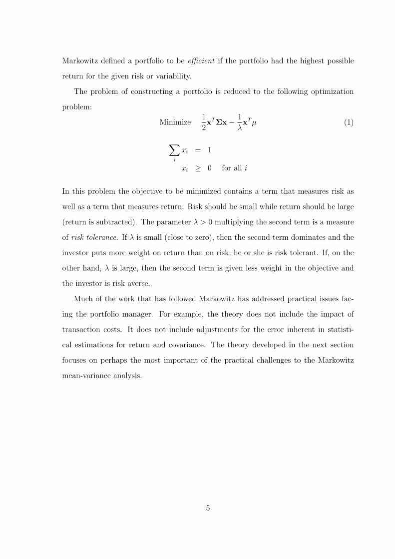
Markowitz defined a portfolio to be efficient if the portfolio had the highest possible

return for the given risk or variability.

The problem of constructing a portfolio is reduced to the following optimization

problem:

Minimize1

2xTΣx− 1

λxT µ (1)

∑i

xi = 1

xi ≥ 0 for all i

In this problem the objective to be minimized contains a term that measures risk as

well as a term that measures return. Risk should be small while return should be large

(return is subtracted). The parameter λ > 0 multiplying the second term is a measure

of risk tolerance. If λ is small (close to zero), then the second term dominates and the

investor puts more weight on return than on risk; he or she is risk tolerant. If, on the

other hand, λ is large, then the second term is given less weight in the objective and

the investor is risk averse.

Much of the work that has followed Markowitz has addressed practical issues fac-

ing the portfolio manager. For example, the theory does not include the impact of

transaction costs. It does not include adjustments for the error inherent in statisti-

cal estimations for return and covariance. The theory developed in the next section

focuses on perhaps the most important of the practical challenges to the Markowitz

mean-variance analysis.

5

3 Definitions of the Information Ratio

Loosely defined, the information ratio (IR) is a measure of portfolio management’s

performance against risk and return relative to a benchmark. The benchmark is a

reference portfolio for active managers and it should be the goal of management to

outperform the benchmark. If an active manager took no risk in a portfolio, his/her

performance would duplicate the results of the benchmark. By taking risks, an ac-

tive portfolio manager has the potential to exceed the performance of the benchmark.

However, taking risks can also backfire, resulting in a loss for the manager’s clients.

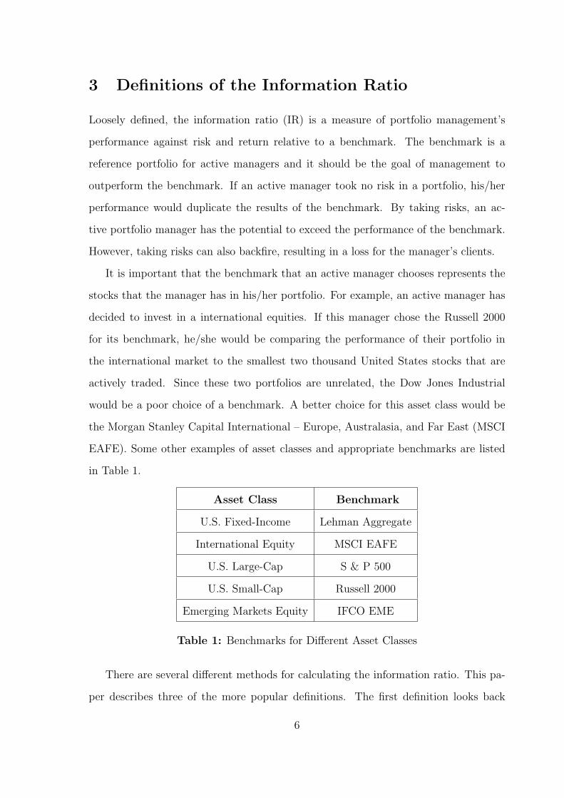
It is important that the benchmark that an active manager chooses represents the

stocks that the manager has in his/her portfolio. For example, an active manager has

decided to invest in a international equities. If this manager chose the Russell 2000

for its benchmark, he/she would be comparing the performance of their portfolio in

the international market to the smallest two thousand United States stocks that are

actively traded. Since these two portfolios are unrelated, the Dow Jones Industrial

would be a poor choice of a benchmark. A better choice for this asset class would be

the Morgan Stanley Capital International – Europe, Australasia, and Far East (MSCI

EAFE). Some other examples of asset classes and appropriate benchmarks are listed

in Table 1.

Asset Class Benchmark

U.S. Fixed-Income Lehman Aggregate

International Equity MSCI EAFE

U.S. Large-Cap S & P 500

U.S. Small-Cap Russell 2000

Emerging Markets Equity IFCO EME

Table 1: Benchmarks for Different Asset Classes

There are several different methods for calculating the information ratio. This pa-

per describes three of the more popular definitions. The first definition looks back

6

at historical data and measures the success (or failure) of the active portfolio man-

ager. The second definition looks into the future and calculates the information ratio

based on forecasted information. The third definition is a theoretical estimation of the

information ratio.

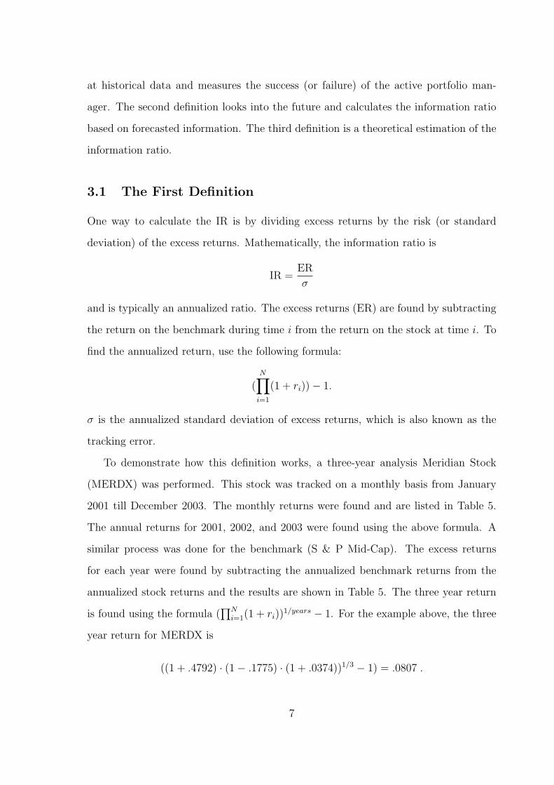
3.1 The First Definition

One way to calculate the IR is by dividing excess returns by the risk (or standard

deviation) of the excess returns. Mathematically, the information ratio is

IR =ER

σ

and is typically an annualized ratio. The excess returns (ER) are found by subtracting

the return on the benchmark during time i from the return on the stock at time i. To

find the annualized return, use the following formula:

(N∏

i=1

(1 + ri))− 1.

σ is the annualized standard deviation of excess returns, which is also known as the

tracking error.

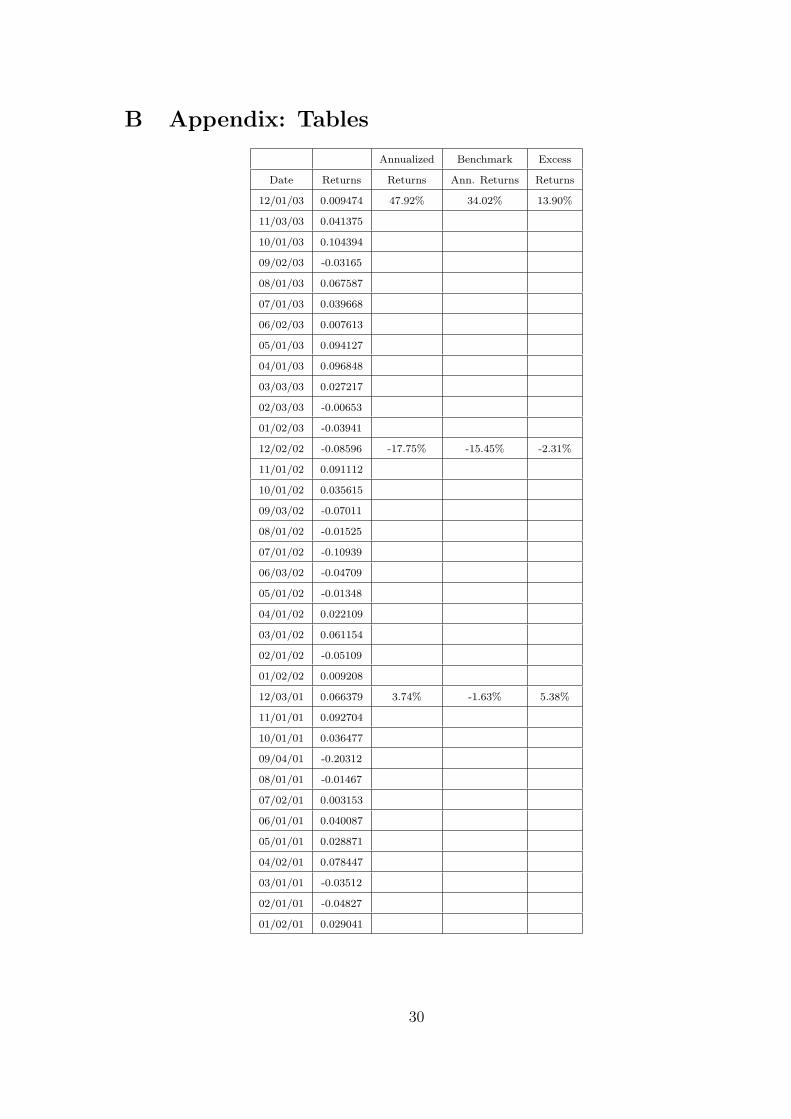
To demonstrate how this definition works, a three-year analysis Meridian Stock

(MERDX) was performed. This stock was tracked on a monthly basis from January

2001 till December 2003. The monthly returns were found and are listed in Table 5.

The annual returns for 2001, 2002, and 2003 were found using the above formula. A

similar process was done for the benchmark (S & P Mid-Cap). The excess returns

for each year were found by subtracting the annualized benchmark returns from the

annualized stock returns and the results are shown in Table 5. The three year return

is found using the formula (∏N

i=1(1 + ri))1/years − 1. For the example above, the three

year return for MERDX is

((1 + .4792) · (1− .1775) · (1 + .0374))1/3 − 1) = .0807 .

7

Using the same formula, the three year return for the S & P Mid-Cap index is 3.69%.

Thus, the excess return is 4.38% (8.07% - 3.69%). The tracking error was found by

taking the standard deviation of the excess returns for 2001, 2002, and 2003 and in

this example, σ = 8.10%. The information ratio is .0438.0810

= .5408.

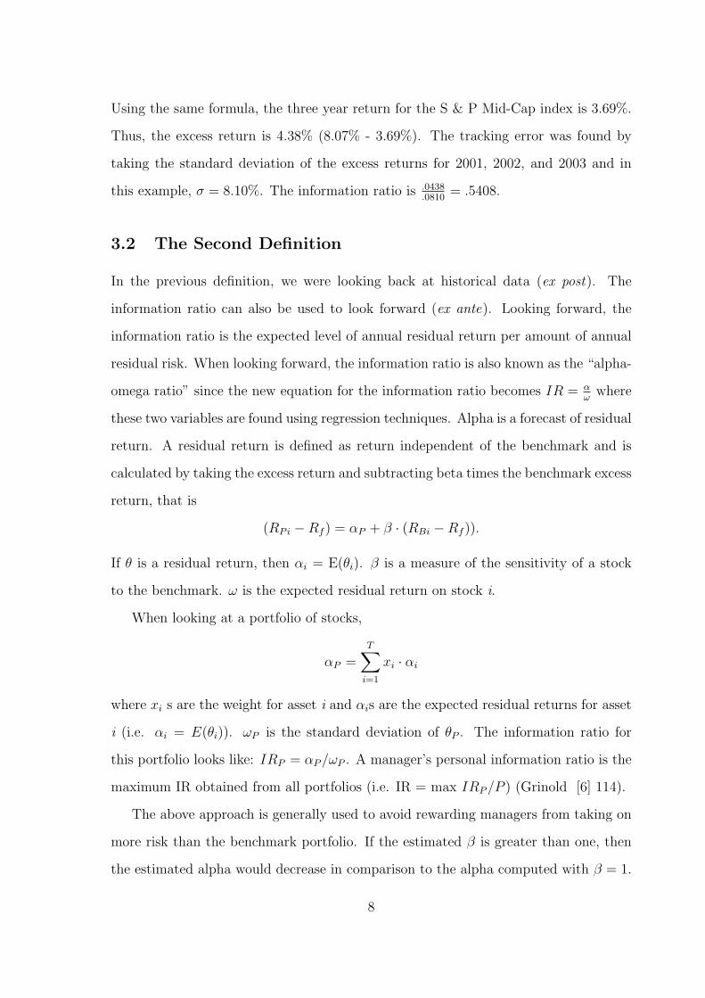
3.2 The Second Definition

In the previous definition, we were looking back at historical data (ex post). The

information ratio can also be used to look forward (ex ante). Looking forward, the

information ratio is the expected level of annual residual return per amount of annual

residual risk. When looking forward, the information ratio is also known as the “alpha-

omega ratio” since the new equation for the information ratio becomes IR = αω

where

these two variables are found using regression techniques. Alpha is a forecast of residual

return. A residual return is defined as return independent of the benchmark and is

calculated by taking the excess return and subtracting beta times the benchmark excess

return, that is

(RPi −Rf ) = αP + β · (RBi −Rf )).

If θ is a residual return, then αi = E(θi). β is a measure of the sensitivity of a stock

to the benchmark. ω is the expected residual return on stock i.

When looking at a portfolio of stocks,

αP =T∑

i=1

xi · αi

where xi s are the weight for asset i and αis are the expected residual returns for asset

i (i.e. αi = E(θi)). ωP is the standard deviation of θP . The information ratio for

this portfolio looks like: IRP = αP /ωP . A manager’s personal information ratio is the

maximum IR obtained from all portfolios (i.e. IR = max IRP /P ) (Grinold [6] 114).

The above approach is generally used to avoid rewarding managers from taking on

more risk than the benchmark portfolio. If the estimated β is greater than one, then

the estimated alpha would decrease in comparison to the alpha computed with β = 1.

8

The estimated ω would be greater than the sigma computed if β = 1 since a β > 1

indicates a higher level of risk. These two changes result in a lower information ratio

for the estimated portfolio. However, if the estimated β is less than one, the overall

result would be an increase in the information ratio due to an increase in the estimated

α and a decrease in ω. Therefore, if the financial manager takes on less risk than

the benchmark, he/she is rewarded with a higher information ratio. Since one of the

key ideas is that the benchmark closely resembles the systematic risk of the estimated

portfolio, it makes sense to fix β = 1. The above information shows how easily the

information ratio can be manipulated to achieve the desired results. It implies that

this version of the information ratio is most useful and accurate when the benchmark

has been carefully chosen to match the style of the financial manager.

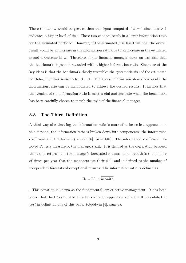
3.3 The Third Definition

A third way of estimating the information ratio is more of a theoretical approach. In

this method, the information ratio is broken down into components: the information

coefficient and the breadth (Grinold [6], page 148). The information coefficient, de-

noted IC, is a measure of the manager’s skill. It is defined as the correlation between

the actual returns and the manager’s forecasted returns. The breadth is the number

of times per year that the managers use their skill and is defined as the number of

independent forecasts of exceptional returns. The information ratio is defined as

IR = IC ·√

breadth

. This equation is known as the fundamental law of active management. It has been

found that the IR calculated ex ante is a rough upper bound for the IR calculated ex

post in definition one of this paper (Goodwin [4], page 3).

9

3.4 A “Good” Information Ratio

With the three definitions given above, it may be confusing for managers to decide

which definition would be best for them to use. Basically, it depends on what type

of data the manager is looking at. If a manager wants to see how well he/she has

performed over time, then the first definition (ex post) is the appropriate one to use.

If, on the other hand, a manager wants to make predictions on how he/ she will do in

the future, then the ex ante (defintion 2) is the most appropriate. The third definition

is used as a rough estimation of the information ratio.

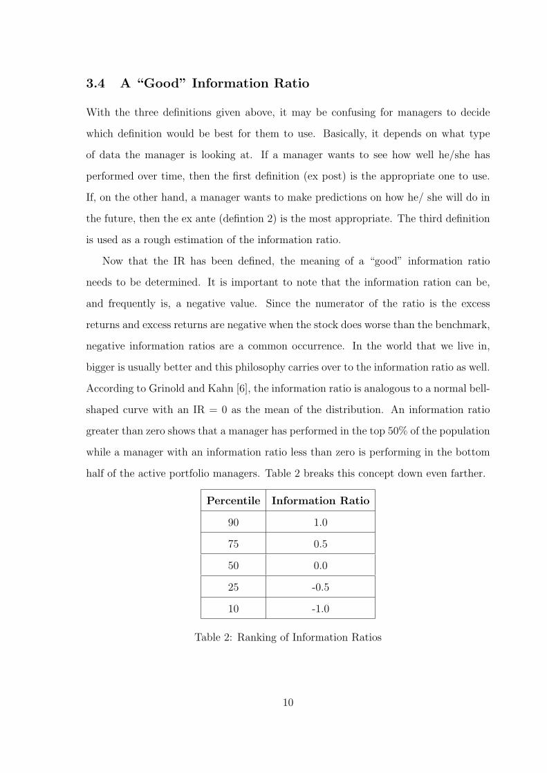
Now that the IR has been defined, the meaning of a “good” information ratio

needs to be determined. It is important to note that the information ration can be,

and frequently is, a negative value. Since the numerator of the ratio is the excess

returns and excess returns are negative when the stock does worse than the benchmark,

negative information ratios are a common occurrence. In the world that we live in,

bigger is usually better and this philosophy carries over to the information ratio as well.

According to Grinold and Kahn [6], the information ratio is analogous to a normal bell-

shaped curve with an IR = 0 as the mean of the distribution. An information ratio

greater than zero shows that a manager has performed in the top 50% of the population

while a manager with an information ratio less than zero is performing in the bottom

half of the active portfolio managers. Table 2 breaks this concept down even farther.

Percentile Information Ratio

90 1.0

75 0.5

50 0.0

25 -0.5

10 -1.0

Table 2: Ranking of Information Ratios

10

This table implies that a manager who is performing in the top quartile has a

“good” information ratio of 0.5. An IR = 1.0 is an exceptional number and it should

be the goal of management to reach this level.

11

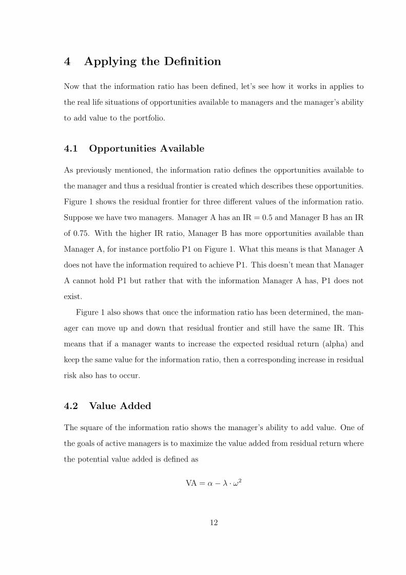
4 Applying the Definition

Now that the information ratio has been defined, let’s see how it works in applies to

the real life situations of opportunities available to managers and the manager’s ability

to add value to the portfolio.

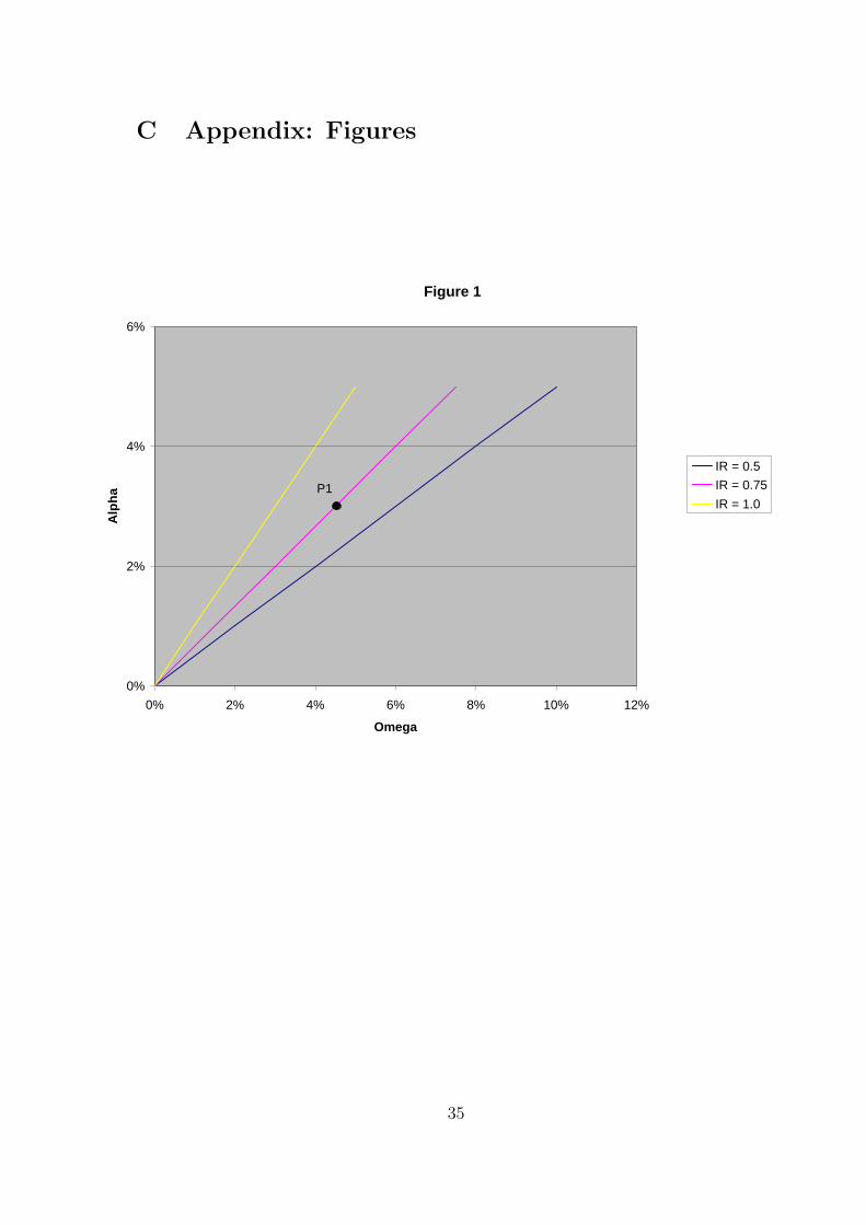
4.1 Opportunities Available

As previously mentioned, the information ratio defines the opportunities available to

the manager and thus a residual frontier is created which describes these opportunities.

Figure 1 shows the residual frontier for three different values of the information ratio.

Suppose we have two managers. Manager A has an IR = 0.5 and Manager B has an IR

of 0.75. With the higher IR ratio, Manager B has more opportunities available than

Manager A, for instance portfolio P1 on Figure 1. What this means is that Manager A

does not have the information required to achieve P1. This doesn’t mean that Manager

A cannot hold P1 but rather that with the information Manager A has, P1 does not

exist.

Figure 1 also shows that once the information ratio has been determined, the man-

ager can move up and down that residual frontier and still have the same IR. This

means that if a manager wants to increase the expected residual return (alpha) and

keep the same value for the information ratio, then a corresponding increase in residual

risk also has to occur.

4.2 Value Added

The square of the information ratio shows the manager’s ability to add value. One of

the goals of active managers is to maximize the value added from residual return where

the potential value added is defined as

VA = α− λ · ω2

12

w here λ is the risk aversion coefficient (Grinold [6], page 119). In this equation, alpha

is found using the ex ante definition of the information ratio, which is a forecast of

residual returns found using regression techniques. By rearranging this “alpha-omega”

definition in terms of alpha and plugging it into the equation of value added given

above, we get

VA = ω · IR− λ · ω2

Now, the problem has been put completely in terms of omega. Since one of the goals

of active management is to maximize value added, the derivative of the above equation

needs to be taken with respect to ω, resulting in

∂V A

∂ω= IR− 2 · λ · ω .

Setting this equation equal to zero gives the maximum value of omega as

ω =IR

2 · λ .

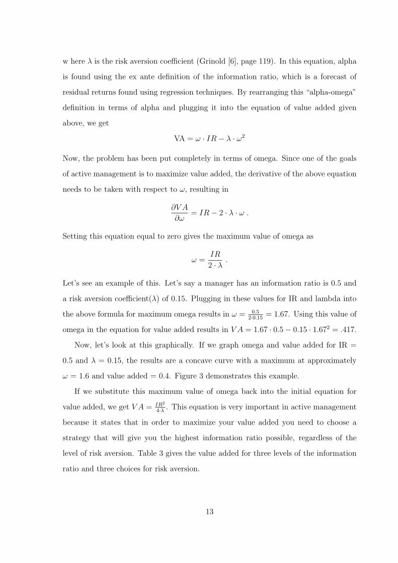
Let’s see an example of this. Let’s say a manager has an information ratio is 0.5 and

a risk aversion coefficient(λ) of 0.15. Plugging in these values for IR and lambda into

the above formula for maximum omega results in ω = 0.52·0.15

= 1.67. Using this value of

omega in the equation for value added results in V A = 1.67 · 0.5− 0.15 · 1.672 = .417.

Now, let’s look at this graphically. If we graph omega and value added for IR =

0.5 and λ = 0.15, the results are a concave curve with a maximum at approximately

ω = 1.6 and value added = 0.4. Figure 3 demonstrates this example.

If we substitute this maximum value of omega back into the initial equation for

value added, we get V A = IR2

4·λ . This equation is very important in active management

because it states that in order to maximize your value added you need to choose a

strategy that will give you the highest information ratio possible, regardless of the

level of risk aversion. Table 3 gives the value added for three levels of the information

ratio and three choices for risk aversion.

13

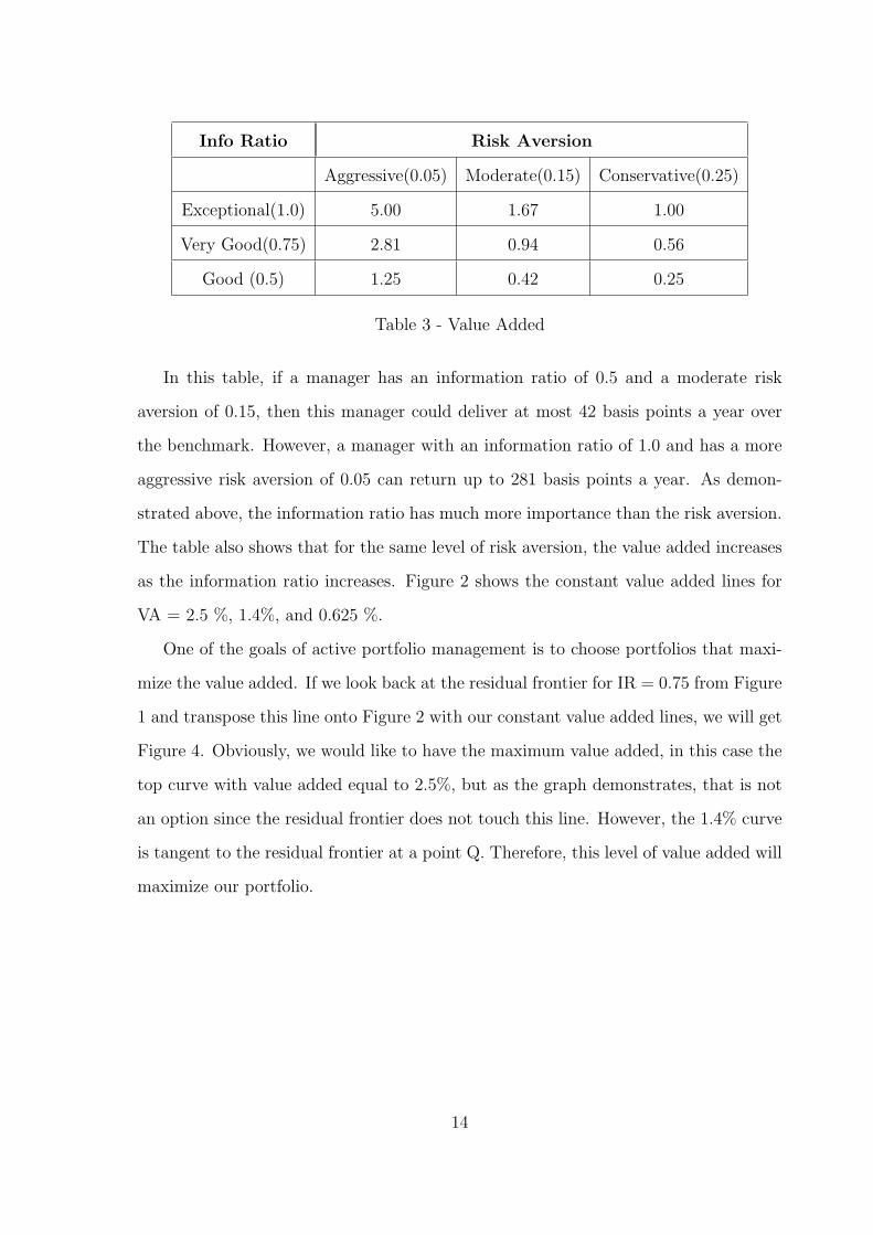
Info Ratio Risk Aversion

Aggressive(0.05) Moderate(0.15) Conservative(0.25)

Exceptional(1.0) 5.00 1.67 1.00

Very Good(0.75) 2.81 0.94 0.56

Good (0.5) 1.25 0.42 0.25

Table 3 - Value Added

In this table, if a manager has an information ratio of 0.5 and a moderate risk

aversion of 0.15, then this manager could deliver at most 42 basis points a year over

the benchmark. However, a manager with an information ratio of 1.0 and has a more

aggressive risk aversion of 0.05 can return up to 281 basis points a year. As demon-

strated above, the information ratio has much more importance than the risk aversion.

The table also shows that for the same level of risk aversion, the value added increases

as the information ratio increases. Figure 2 shows the constant value added lines for

VA = 2.5 %, 1.4%, and 0.625 %.

One of the goals of active portfolio management is to choose portfolios that maxi-

mize the value added. If we look back at the residual frontier for IR = 0.75 from Figure

1 and transpose this line onto Figure 2 with our constant value added lines, we will get

Figure 4. Obviously, we would like to have the maximum value added, in this case the

top curve with value added equal to 2.5%, but as the graph demonstrates, that is not

an option since the residual frontier does not touch this line. However, the 1.4% curve

is tangent to the residual frontier at a point Q. Therefore, this level of value added will

maximize our portfolio.

14

5 Negative Impacts on the Information Ratio

There are several things that could have a negative impact on the information ratio.

Two items that we will take a deeper look at are negative excess returns and transaction

costs.

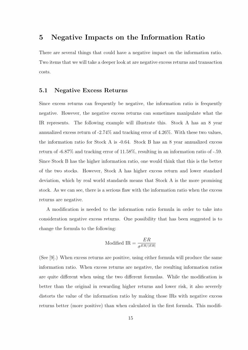
5.1 Negative Excess Returns

Since excess returns can frequently be negative, the information ratio is frequently

negative. However, the negative excess returns can sometimes manipulate what the

IR represents. The following example will illustrate this. Stock A has an 8 year

annualized excess return of -2.74% and tracking error of 4.26%. With these two values,

the information ratio for Stock A is -0.64. Stock B has an 8 year annualized excess

return of -6.87% and tracking error of 11.58%, resulting in an information ratio of -.59.

Since Stock B has the higher information ratio, one would think that this is the better

of the two stocks. However, Stock A has higher excess return and lower standard

deviation, which by real world standards means that Stock A is the more promising

stock. As we can see, there is a serious flaw with the information ratio when the excess

returns are negative.

A modification is needed to the information ratio formula in order to take into

consideration negative excess returns. One possibility that has been suggested is to

change the formula to the following:

Modified IR =ER

σER/|ER|

(See [9].) When excess returns are positive, using either formula will produce the same

information ratio. When excess returns are negative, the resulting information ratios

are quite different when using the two different formulas. While the modification is

better than the original in rewarding higher returns and lower risk, it also severely

distorts the value of the information ratio by making those IRs with negative excess

returns better (more positive) than when calculated in the first formula. This modifi-

15

cation can be used to rank stocks but shouldn’t be used to put a numerical value on a

portfolio manager’s performance.

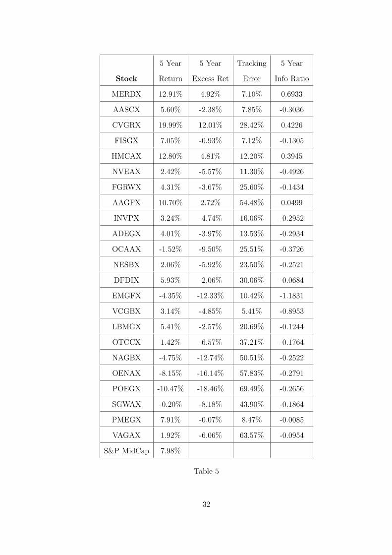
To illustrate this point, a five year study of twenty-five mutual funds was conducted.

All of the mutual funds were randomly chosen from the Mid-Cap Growth Asset Class

and the benchmark used was the S & P MidCap 400. Two of the mutual funds had

to be thrown out due to insufficient data. A brief summary of all the mutual funds

used is given in the appendix. During the five year time period, the annual returns and

excess returns were calculated. Then, the five year return, five year excess return, and

tracking error were computed and the resulting information ratios were found. The

results are found in Table 5 on page 32.

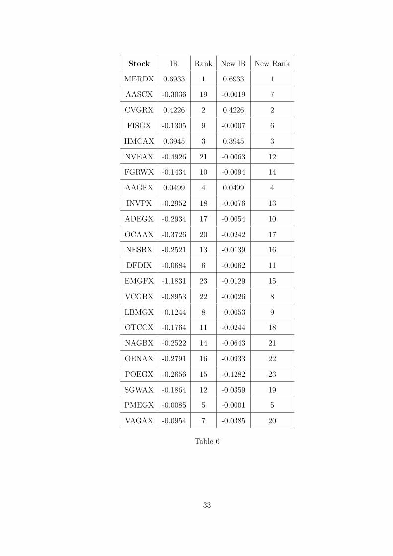
Using the modification formula described above, the new Information Ratios were

found for the same group of stocks. The stocks were ranked according to their infor-

mation ratios with 1 being the highest and 23 the lowest. The results are listed in

Table 6 on page 33. As seen in this table, the new information ratios are significantly

different from the original ratios. There needs to be a way to compromise between

the two methods so that the information ratios are more realistic as with the original

ratios but have the ranking scheme of the modified information ratios.

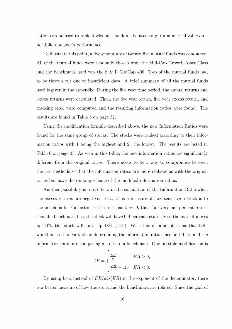
Another possibility is to use beta in the calculation of the Information Ratio when

the excess returns are negative. Beta, β, is a measure of how sensitive a stock is to

the benchmark. For instance if a stock has β = .9, then for every one percent return

that the benchmark has, the stock will have 0.9 percent return. So if the market moves

up 20%, this stock will move up 18% (.2·.9). With this in mind, it seems that beta

would be a useful variable in determining the information ratio since both beta and the

information ratio are comparing a stock to a benchmark. One possible modification is

IR =

ERσ

ER > 0,

ERσ−β − .15 ER < 0.

By using beta instead of ER/abs(ER) in the exponent of the denominator, there

is a better measure of how the stock and the benchmark are related. Since the goal of

16

the information is to show how well or poorly a manager is performing compared to

a benchmark then it is a reasonable assumption to use a variable that measures that

relationship. Beta is a perfect choice for that. The use of the scalar -.15 is to make the

newly calculated information ratios more realistic. In the first modification, almost all

of the new information ratios got better in that they became closer to zero. The main

objective of the modification is to reward managers with higher excess returns and lower

risk and penalize those with lower excess returns and higher levels of risk. Thus, the

modification should result in information ratios that more negative for those managers

who have poor returns are have high levels of risk. By imposing a constant penalty

of -.15 to all ratios with negative excess returns, there are more realistic information

ratios but the ranking of the information ratios would not change since the ranking is

decided by the first part of the formula ( ERσ−β ).

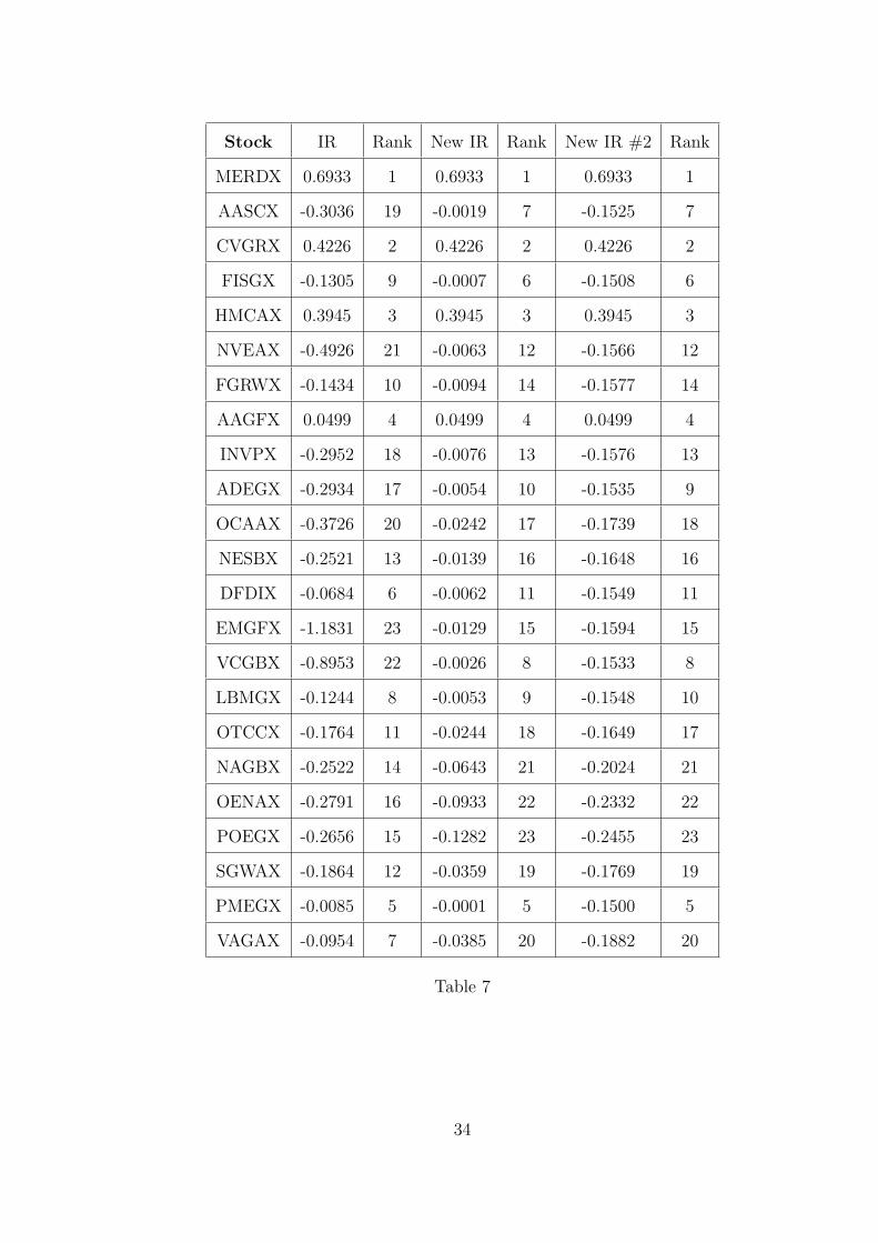
This new modification was applied to the same group of mutual funds given in the

previous two examples. Five year betas were found for each stock using information

from the Yahoo!Finance website. Table 6 shows the results of applying all three for-

mulas to the data. As seen in the table, the third formula gives almost the exact same

rankings as the second formula but has information ratios that more closely resemble

those in the first formula.

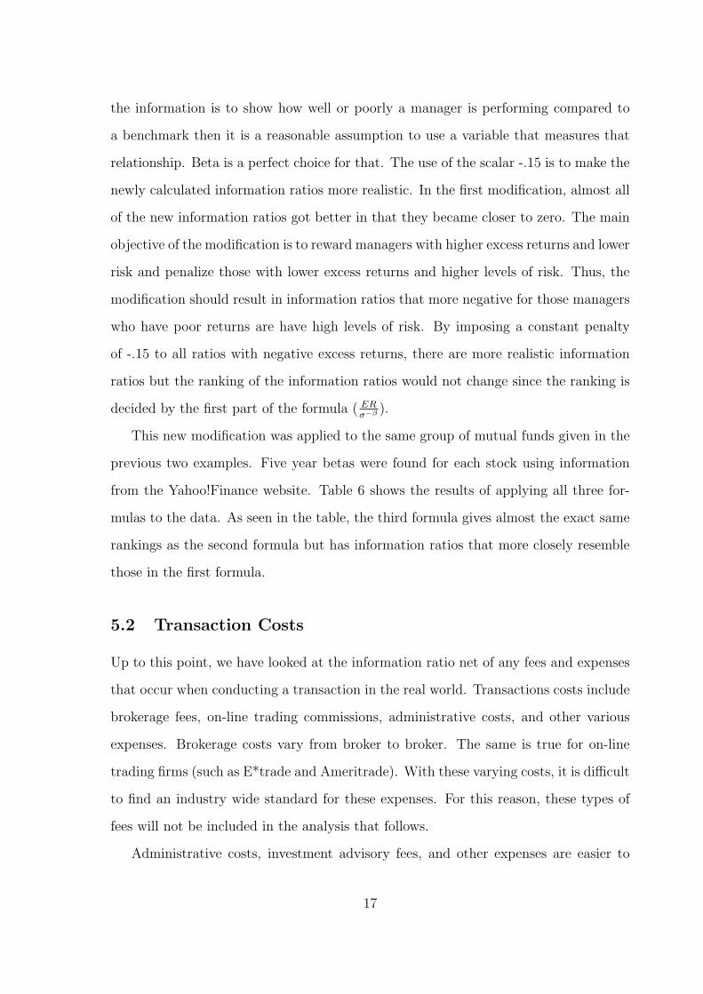
5.2 Transaction Costs

Up to this point, we have looked at the information ratio net of any fees and expenses

that occur when conducting a transaction in the real world. Transactions costs include

brokerage fees, on-line trading commissions, administrative costs, and other various

expenses. Brokerage costs vary from broker to broker. The same is true for on-line

trading firms (such as E*trade and Ameritrade). With these varying costs, it is difficult

to find an industry wide standard for these expenses. For this reason, these types of

fees will not be included in the analysis that follows.

Administrative costs, investment advisory fees, and other expenses are easier to

17

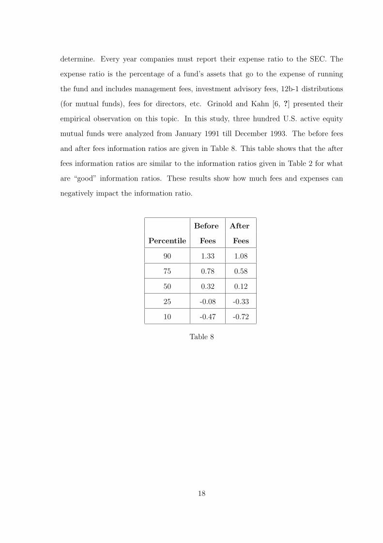
determine. Every year companies must report their expense ratio to the SEC. The

expense ratio is the percentage of a fund’s assets that go to the expense of running

the fund and includes management fees, investment advisory fees, 12b-1 distributions

(for mutual funds), fees for directors, etc. Grinold and Kahn [6, ?] presented their

empirical observation on this topic. In this study, three hundred U.S. active equity

mutual funds were analyzed from January 1991 till December 1993. The before fees

and after fees information ratios are given in Table 8. This table shows that the after

fees information ratios are similar to the information ratios given in Table 2 for what

are “good” information ratios. These results show how much fees and expenses can

negatively impact the information ratio.

Before After

Percentile Fees Fees

90 1.33 1.08

75 0.78 0.58

50 0.32 0.12

25 -0.08 -0.33

10 -0.47 -0.72

Table 8

18

6 Comparison to Other Ratios

The information ratio can be compared to several other statistical performance mea-

sures such as the t-statistic and the Sharpe ratio.

6.1 IR vs. t-statistic

Looking ex post, the information ratio can be compared to the t-statistic since there

is a connection between the statistical significance of excess returns and statistical

significance of an information ratio. As a refresher from statistics, here is a quick

review of this statistical value. The t-statistic has a t distribution with T - 1 degrees of

freedom where T is the number of time periods. This statistic is based on a hypothesis

test and the result of this test can be determined by standard t-tables. When testing

the statistical significance of the information ratio, one would choose a hypothesis

test where the null hypothesis would be that the excess returns over the benchmark

portfolio would be zero and the alternative hypothesis would be that the excess returns

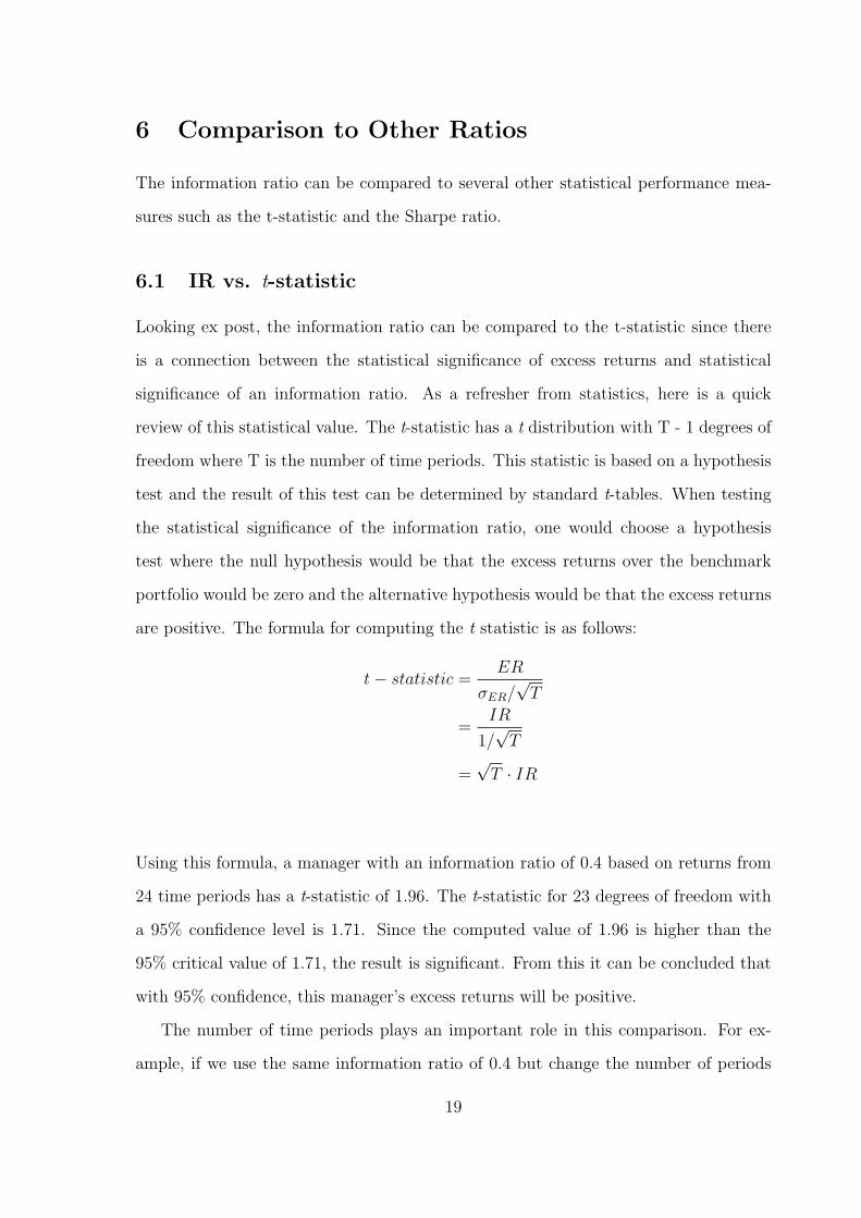
are positive. The formula for computing the t statistic is as follows:

t − statistic =ER

σER/√

T

=IR

1/√

T

=√

T · IR

Using this formula, a manager with an information ratio of 0.4 based on returns from

24 time periods has a t-statistic of 1.96. The t-statistic for 23 degrees of freedom with

a 95% confidence level is 1.71. Since the computed value of 1.96 is higher than the

95% critical value of 1.71, the result is significant. From this it can be concluded that

with 95% confidence, this manager’s excess returns will be positive.

The number of time periods plays an important role in this comparison. For ex-

ample, if we use the same information ratio of 0.4 but change the number of periods

19

to nine, the corresponding t-statistic is 1.2 but the 95% confidence value is 1.86 for

eight degrees of freedom. Thus, the result is not significant in this example. This

demonstrates that statistical testing can show how confident a manager can be with

the calculated information ratio but the length of time that the IR was calculated over

plays a very important role in the significance of the t-test.

6.2 IR vs. Sharpe Ratio

Another ratio that is closely related to the information ratio is the Sharpe ratio. This

statistic was introduced by William Sharpe in 1966 and is defined as the excess return

on a portfolio over a risk-free asset, such as a T-bill, divided by the risk of the portfolio:

SR =ERrf

σ.

The exact connection between the Sharpe ratio and the IR is quite controversial.

Sharpe states that the information ratio is a “generalized Sharpe ratio” [15]. Oth-

ers state that the Sharpe ratio is actually the squared information ratio. While there

is a lot of confusion over the actual connection between these two ratios, you can see

that there is a relationship between these two ratios.

20

7 IR Improvement Techniques

There are several things to keep in mind when using the information ratio. First,

consistency is key. In order to have the most accurate information ratio possible, the

same type of data most be used for both the funds and the benchmark. If daily returns

are used for the funds, then daily returns need to be used for the benchmark. If different

types of returns are used (i.e. weekly returns for funds and monthly returns for the

benchmark) then the information ratio could be negatively affected.

It is also important that the funds being analyzed are mostly from the same asset

class. By choosing stocks from different asset classes it becomes a greater challenge to

find a benchmark that accurately reflects both asset classes, thus resulting in a lower

information ratio. That leads us to the next improvement technique, choosing a bench-

mark that corresponds to the asset class the funds are in. If a poor choice of benchmark

is picked, the data can easily be manipulated to produce a higher information ratio

than in reality.

Another way to improve the information ratio is just to practice, practice, practice.

Take a look back at the third definition of the information ratio given in this paper.

Here, the IR is defined as skill (IC) multiplied by the square root of breadth. It can be

difficult to increase your skill value so in order to increase the information ratio using

this definition, breadth has to be increased. Since breadth is the number of times that

a manager uses his/her skill, it is easy for breadth to be increased. Also, by using skill

over and over to increase breadth, a manager is inevitably going to increase their skill

level so it is a win-win situation.

Another strategy is given by Kahn and takes into consideration before and after fees

information ratios (Kahn [10]). Kahn’s paper focuses on bond managers but his ideas

can be applied to active portfolio managers as well. In his approach, estimates are given

for fees/expenses and excess returns. For instance, let’s say a manager thinks he/she

will have fees/expenses of 40 basis points and excess returns of 75 basis points, net of

fees and expenses during the next time period. With these estimates, this manager

21

would have to produce 115 (40 + 75) basis points of excess returns, gross of fees and

expenses. If this manager is a top-quartile manager, then his/her information ratio is

around 0.5. In order for this manager to maintain that information ratio, he/she will

have to take on 230 (115/0.5) basis points of active risk. Now let’s look at this from a

slightly different angle. Let’s say this same manager wants to increase the information

ratio from 0.5 to 0.6. To achieve this improved information ratio, the manager has

three possible options:(a) increase excess returns (gross of fees and expenses) to 138

and keep the same risk level of 230, (b) increase the level of risk to 192 and keep the

same target of excess returns at 115, or (c) slightly increase both of these two variables

(one possibility is excess returns equal to 125 and risk equal to 208). Deciding which

of the strategies to implement depends on a variety of things including the manager’s

individual strengths and weaknesses and the market conditions at that time.

22

8 Conclusion

As its name suggests, the information ratio can be a very “informative” tool. It also

can be a deceiving tool. There are both advantages and disadvantages for using this

statistic. On one hand, the information ratio can provide some insight into how well

an active portfolio manager is performing with respect to a chosen benchmark. On the

other hand, transaction costs and negative excess returns can significantly impact the

information ratio in unflattering ways.

In this paper, three different definitions of the information ratio are given. While

each one is theoretically correct, it is not clear whether one definition is better than any

of the other definitions. The Brandes Institute [1] recommends defining an industry-

wide set of standards to help clear up the confusion. As of this time, no such regulations

have been implemented but it is something that should further investigated.

There are several other aspects of the information ratio that could be topics of future

research projects. One is finding a better way to handle negative excess returns. As

shown in this paper, the negative excess returns can manipulate the information ratio.

Two modifications were given regarding this problem but further research might give

and improved modification that would work better than the two given here. Another

area of further research is finding a clearer relationship between the information ratio

and the Sharpe ratio. A brief look at the connection between these two ratios was

given in this paper but more research is needed to find a more concise relationship the

information and Sharpe ratios.

Overall, the information ratio can provide a good measurement of how a portfolio

manager is performing but should not be the only statistic used due to some ambiguities

in calculating this statistic.

23

A Appendix: Stock Summaries

(All information provided by Yahoo!Finance)

MERDX - Meridian Growth Fund seeks long-term growth of capital. The fund

invests primarily in equity securities. Investments may include common stocks, con-

vertible securities, and warrants. When evaluating companies, the advisor considers

such factors as growth rates relative to P/E ratios, financial strength, quality of man-

agement, and relative value compared with other investments. The fund may invest

up to 25% of assets in companies with fewer than three years of operating history. It

may also invest in securities of foreign issuers.

AASCX - Thrivent Mid Cap Stock Fund seeks long-term capital growth. The

fund normally invests at least 65% of assets in mid-sized company stocks. The advi-

sors of the fund define mid-sized companies as those with market capitalization ranging

from $100 million to $7.5 billion, within this category the advisor generally will focus

on companies with market capitalizations ranging from $500 million to $3.5 billion. It

may invest the balance in additional mid-cap stocks, large-cap stocks, and convertibles.

CVGRX - Calamos Growth Fund seeks long-term capital growth. The fund nor-

mally invests in common stocks, though there are no limitations on the amount of

assets that may be allocated to various types of securities. The investment-selection

process emphasizes earnings-growth potential coupled with financial strength and sta-

bility. The fund may invest no more than 5% of assets in the securities of unseasoned

issuers. It may also invest up to 25% of assets in foreign securities and may engage in

various futures and options strategies.

FISGX - First American Mid Cap Growth Opportunities Fund seeks capital ap-

preciation. The fund normally invests at least 80% of assets in common stocks of

mid-capitalization companies. These are defined as companies that constitute the S &

24

P MidCap 400 Index and with market capitalizations between $278 million and $10.9

billion. The fund may invest up to 25% of assets in foreign securities.

HMCAX - Heritage Mid Cap Stock Fund seeks long-term capital appreciation.

The fund normally invests at least 80% of assets in equity securities of medium capi-

talization companies. It may invest in common and preferred stocks, warrants or rights

exercisable into common or preferred stock, and securities convertible into equities. The

fund may invest up to 100% of assets in high-quality and short-term debt instruments.

It may engage in short-term transactions under various market conditions to a greater

extent than certain other mutual funds with similar investment objectives.

NVEAX - Wells Fargo Growth Equity Fund seeks long-term capital growth while

moderating annual return volatility. The fund normally invests at least 65% of assets

in equities. It divides assets among three equity investment styles represented by other

Norwest funds: 35% in Large Company Growth, which invests in issuers with market

caps of at least $500 million and with unrecognized value; 35% in Small Company

Growth, which invests in issuers with market caps of $750 million or less; and 30% in

International.

FGRWX - Hartford Growth Opportunities Fund seeks short and long-term capital

appreciation. The fund primarily invests in equity securities covering a broad range of

industries, companies and market capitalizations. It may invest up to 20% of assets in

foreign issuers and non-dollar securities.

AAGFX - AIM Aggressive Growth Fund seeks long-term growth of capital. The

fund invests in common stocks of companies whose earnings the fund’s portfolio man-

agers expect to grow more than 15% per year. It typically invests in securities of small

and medium-sized growth companies. The fund may also invest up to 25% of assets in

25

foreign securities and may hold a portion of assets in cash or cash equivalents.

INVPX - AXP Equity Select Fund seeks growth of capital. The fund invests at

least 80% of assets in equity securities. It primarily invests in growth stocks of medium-

sized companies. It may also invest in small- and large-sized companies. Management

chooses equity investments by identifying companies with effective management, finan-

cial strength, growth potential and a competitive market position.

ADEGX - Advance Capital I Equity Growth Fund seeks long-term capital growth.

The fund normally invests at least 65% of assets in equities, not including stock in-

dex futures and options. It invests primarily in small growth companies with market

capitalizations of $1.5 billion or less. Management selects companies that are in the

developmental stage of its life cycle and that have demonstrated or are expected to

achieve long-term earnings growth which reaches new highs per share during each ma-

jor business cycle. The fund may invest the balance in preferred stocks, convertible

debt securities, stock index futures and options.

OCAAX - BB&T Mid Cap Growth Fund seeks long-term growth of capital. The

fund normally invests at least 65% of assets in equities issued by companies with es-

tablished growth records. These companies typically have capitalizations in excess of

$1 billion and revenues in excess of $500 million. To select investments, the advisor

also considers development of new products, business restructuring, new management,

and the potential for increased institutional ownership.

NESBX - CDC Nvest Star Advisers Fund seeks long-term growth of capital. The

Fund primarily invests in equity securities. It may also invest in securities offered

in initial public offerings (IPOs), real estate investment trusts (REITs), convertible

preferred stock and convertible debt securities, fixed-income securities, including U.S.

26

government bonds and lower-quality bonds. The Fund may also invest in options enter

into futures, swap contracts and currency hedging transactions and hold securities of

foreign issuers.

DFDIX - Delaware Growth Opportunities Fund seeks long-term capital growth.

The fund primarily invests in equities that are selected based on the financial strength

of the company, the expertise of its management, the growth potential of the company,

and the growth potential of the industry itself. The fund may invest up to 25% of

assets in foreign securities.

EMGFX - Eaton Vance Growth Fund seeks capital growth; income is a secondary

consideration. The fund primarily invests in common stocks of U.S. growth companies.

Although it invests primarily in domestic companies, the fund may invest up to 25%

of assets in foreign companies. It may at times engage in derivative transactions (such

as futures contracts and options) to protect against price declines, to enhance return

or as a substitute for the purchase or sale of securities.

VCGBX - JP Morgan Capital Growth Fund seeks long-term capital growth. The

fund normally invests at least 80% of assets in equity securities of companies with mar-

ket capitalizations equal to those within the universe of Russell Midcap Growth Index

at the time of purchase. It may invest in common stocks, preferred stocks, convertible

securities, depositary receipts and warrants to buy common stocks. The fund may also

use derivatives for hedging. It is nondiversified.

LBMGX - Thrivent Mid Cap Growth Fund seeks long-term growth of capital. The

fund normally invests at least 80% of assets in common stocks issued by companies

with market capitalizations between $1 billion and $5 billion. Management seeks to

identify companies that have a track record of earnings growth or the potential for

27

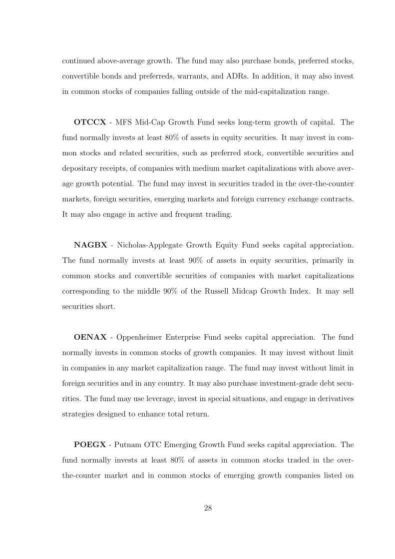
continued above-average growth. The fund may also purchase bonds, preferred stocks,

convertible bonds and preferreds, warrants, and ADRs. In addition, it may also invest

in common stocks of companies falling outside of the mid-capitalization range.

OTCCX - MFS Mid-Cap Growth Fund seeks long-term growth of capital. The

fund normally invests at least 80% of assets in equity securities. It may invest in com-

mon stocks and related securities, such as preferred stock, convertible securities and

depositary receipts, of companies with medium market capitalizations with above aver-

age growth potential. The fund may invest in securities traded in the over-the-counter

markets, foreign securities, emerging markets and foreign currency exchange contracts.

It may also engage in active and frequent trading.

NAGBX - Nicholas-Applegate Growth Equity Fund seeks capital appreciation.

The fund normally invests at least 90% of assets in equity securities, primarily in

common stocks and convertible securities of companies with market capitalizations

corresponding to the middle 90% of the Russell Midcap Growth Index. It may sell

securities short.

OENAX - Oppenheimer Enterprise Fund seeks capital appreciation. The fund

normally invests in common stocks of growth companies. It may invest without limit

in companies in any market capitalization range. The fund may invest without limit in

foreign securities and in any country. It may also purchase investment-grade debt secu-

rities. The fund may use leverage, invest in special situations, and engage in derivatives

strategies designed to enhance total return.

POEGX - Putnam OTC Emerging Growth Fund seeks capital appreciation. The

fund normally invests at least 80% of assets in common stocks traded in the over-

the-counter market and in common stocks of emerging growth companies listed on

28

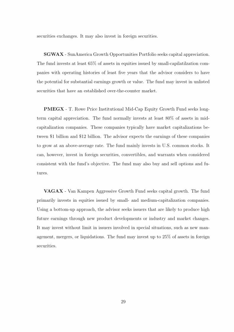
securities exchanges. It may also invest in foreign securities.

SGWAX - SunAmerica Growth Opportunities Portfolio seeks capital appreciation.

The fund invests at least 65% of assets in equities issued by small-capilatilzation com-

panies with operating histories of least five years that the advisor considers to have

the potential for substantial earnings growth or value. The fund may invest in unlisted

securities that have an established over-the-counter market.

PMEGX - T. Rowe Price Institutional Mid-Cap Equity Growth Fund seeks long-

term capital appreciation. The fund normally invests at least 80% of assets in mid-

capitalization companies. These companies typically have market capitalizations be-

tween $1 billion and $12 billion. The advisor expects the earnings of these companies

to grow at an above-average rate. The fund mainly invests in U.S. common stocks. It

can, however, invest in foreign securities, convertibles, and warrants when considered

consistent with the fund’s objective. The fund may also buy and sell options and fu-

tures.

VAGAX - Van Kampen Aggressive Growth Fund seeks capital growth. The fund

primarily invests in equities issued by small- and medium-capitalization companies.

Using a bottom-up approach, the advisor seeks issuers that are likely to produce high

future earnings through new product developments or industry and market changes.

It may invest without limit in issuers involved in special situations, such as new man-

agement, mergers, or liquidations. The fund may invest up to 25% of assets in foreign

securities.

29

B Appendix: Tables

Annualized Benchmark Excess

Date Returns Returns Ann. Returns Returns

12/01/03 0.009474 47.92% 34.02% 13.90%

11/03/03 0.041375

10/01/03 0.104394

09/02/03 -0.03165

08/01/03 0.067587

07/01/03 0.039668

06/02/03 0.007613

05/01/03 0.094127

04/01/03 0.096848

03/03/03 0.027217

02/03/03 -0.00653

01/02/03 -0.03941

12/02/02 -0.08596 -17.75% -15.45% -2.31%

11/01/02 0.091112

10/01/02 0.035615

09/03/02 -0.07011

08/01/02 -0.01525

07/01/02 -0.10939

06/03/02 -0.04709

05/01/02 -0.01348

04/01/02 0.022109

03/01/02 0.061154

02/01/02 -0.05109

01/02/02 0.009208

12/03/01 0.066379 3.74% -1.63% 5.38%

11/01/01 0.092704

10/01/01 0.036477

09/04/01 -0.20312

08/01/01 -0.01467

07/02/01 0.003153

06/01/01 0.040087

05/01/01 0.028871

04/02/01 0.078447

03/01/01 -0.03512

02/01/01 -0.04827

01/02/01 0.029041

30

3-Year 3-Year 3-Year Tracking 3-Year

Return Benchmark Excess Error IR

8.07% 3.69% 4.38% 8.10% 0.5408

Table 4

31

5 Year 5 Year Tracking 5 Year

Stock Return Excess Ret Error Info Ratio

MERDX 12.91% 4.92% 7.10% 0.6933

AASCX 5.60% -2.38% 7.85% -0.3036

CVGRX 19.99% 12.01% 28.42% 0.4226

FISGX 7.05% -0.93% 7.12% -0.1305

HMCAX 12.80% 4.81% 12.20% 0.3945

NVEAX 2.42% -5.57% 11.30% -0.4926

FGRWX 4.31% -3.67% 25.60% -0.1434

AAGFX 10.70% 2.72% 54.48% 0.0499

INVPX 3.24% -4.74% 16.06% -0.2952

ADEGX 4.01% -3.97% 13.53% -0.2934

OCAAX -1.52% -9.50% 25.51% -0.3726

NESBX 2.06% -5.92% 23.50% -0.2521

DFDIX 5.93% -2.06% 30.06% -0.0684

EMGFX -4.35% -12.33% 10.42% -1.1831

VCGBX 3.14% -4.85% 5.41% -0.8953

LBMGX 5.41% -2.57% 20.69% -0.1244

OTCCX 1.42% -6.57% 37.21% -0.1764

NAGBX -4.75% -12.74% 50.51% -0.2522

OENAX -8.15% -16.14% 57.83% -0.2791

POEGX -10.47% -18.46% 69.49% -0.2656

SGWAX -0.20% -8.18% 43.90% -0.1864

PMEGX 7.91% -0.07% 8.47% -0.0085

VAGAX 1.92% -6.06% 63.57% -0.0954

S&P MidCap 7.98%

Table 5

32

Stock IR Rank New IR New Rank

MERDX 0.6933 1 0.6933 1

AASCX -0.3036 19 -0.0019 7

CVGRX 0.4226 2 0.4226 2

FISGX -0.1305 9 -0.0007 6

HMCAX 0.3945 3 0.3945 3

NVEAX -0.4926 21 -0.0063 12

FGRWX -0.1434 10 -0.0094 14

AAGFX 0.0499 4 0.0499 4

INVPX -0.2952 18 -0.0076 13

ADEGX -0.2934 17 -0.0054 10

OCAAX -0.3726 20 -0.0242 17

NESBX -0.2521 13 -0.0139 16

DFDIX -0.0684 6 -0.0062 11

EMGFX -1.1831 23 -0.0129 15

VCGBX -0.8953 22 -0.0026 8

LBMGX -0.1244 8 -0.0053 9

OTCCX -0.1764 11 -0.0244 18

NAGBX -0.2522 14 -0.0643 21

OENAX -0.2791 16 -0.0933 22

POEGX -0.2656 15 -0.1282 23

SGWAX -0.1864 12 -0.0359 19

PMEGX -0.0085 5 -0.0001 5

VAGAX -0.0954 7 -0.0385 20

Table 6

33

Stock IR Rank New IR Rank New IR #2 Rank

MERDX 0.6933 1 0.6933 1 0.6933 1

AASCX -0.3036 19 -0.0019 7 -0.1525 7

CVGRX 0.4226 2 0.4226 2 0.4226 2

FISGX -0.1305 9 -0.0007 6 -0.1508 6

HMCAX 0.3945 3 0.3945 3 0.3945 3

NVEAX -0.4926 21 -0.0063 12 -0.1566 12

FGRWX -0.1434 10 -0.0094 14 -0.1577 14

AAGFX 0.0499 4 0.0499 4 0.0499 4

INVPX -0.2952 18 -0.0076 13 -0.1576 13

ADEGX -0.2934 17 -0.0054 10 -0.1535 9

OCAAX -0.3726 20 -0.0242 17 -0.1739 18

NESBX -0.2521 13 -0.0139 16 -0.1648 16

DFDIX -0.0684 6 -0.0062 11 -0.1549 11

EMGFX -1.1831 23 -0.0129 15 -0.1594 15

VCGBX -0.8953 22 -0.0026 8 -0.1533 8

LBMGX -0.1244 8 -0.0053 9 -0.1548 10

OTCCX -0.1764 11 -0.0244 18 -0.1649 17

NAGBX -0.2522 14 -0.0643 21 -0.2024 21

OENAX -0.2791 16 -0.0933 22 -0.2332 22

POEGX -0.2656 15 -0.1282 23 -0.2455 23

SGWAX -0.1864 12 -0.0359 19 -0.1769 19

PMEGX -0.0085 5 -0.0001 5 -0.1500 5

VAGAX -0.0954 7 -0.0385 20 -0.1882 20

Table 7

34

C Appendix: Figures

Figure 1

0%

2%

4%

6%

0% 2% 4% 6% 8% 10% 12%

Omega

Alp

ha

IR = 0.5

IR = 0.75

IR = 1.0P1

35

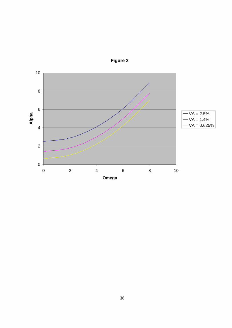
Figure 2

0

2

4

6

8

10

0 2 4 6 8 10

Omega

Alp

ha VA = 2.5%

VA = 1.4%VA = 0.625%

36

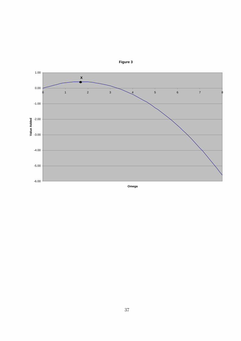
Figure 3

-6.00

-5.00

-4.00

-3.00

-2.00

-1.00

0.00

1.00

0 1 2 3 4 5 6 7 8

Omega

Val

ue

Ad

ded

X

37

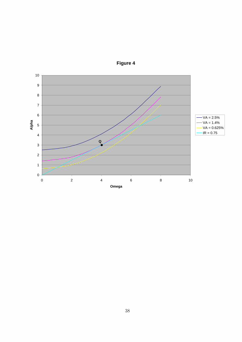
Figure 4

0

1

2

3

4

5

6

7

8

9

10

0 2 4 6 8 10

Omega

Alp

ha

VA = 2.5%VA = 1.4%VA = 0.625%IR = 0.75

Q

38

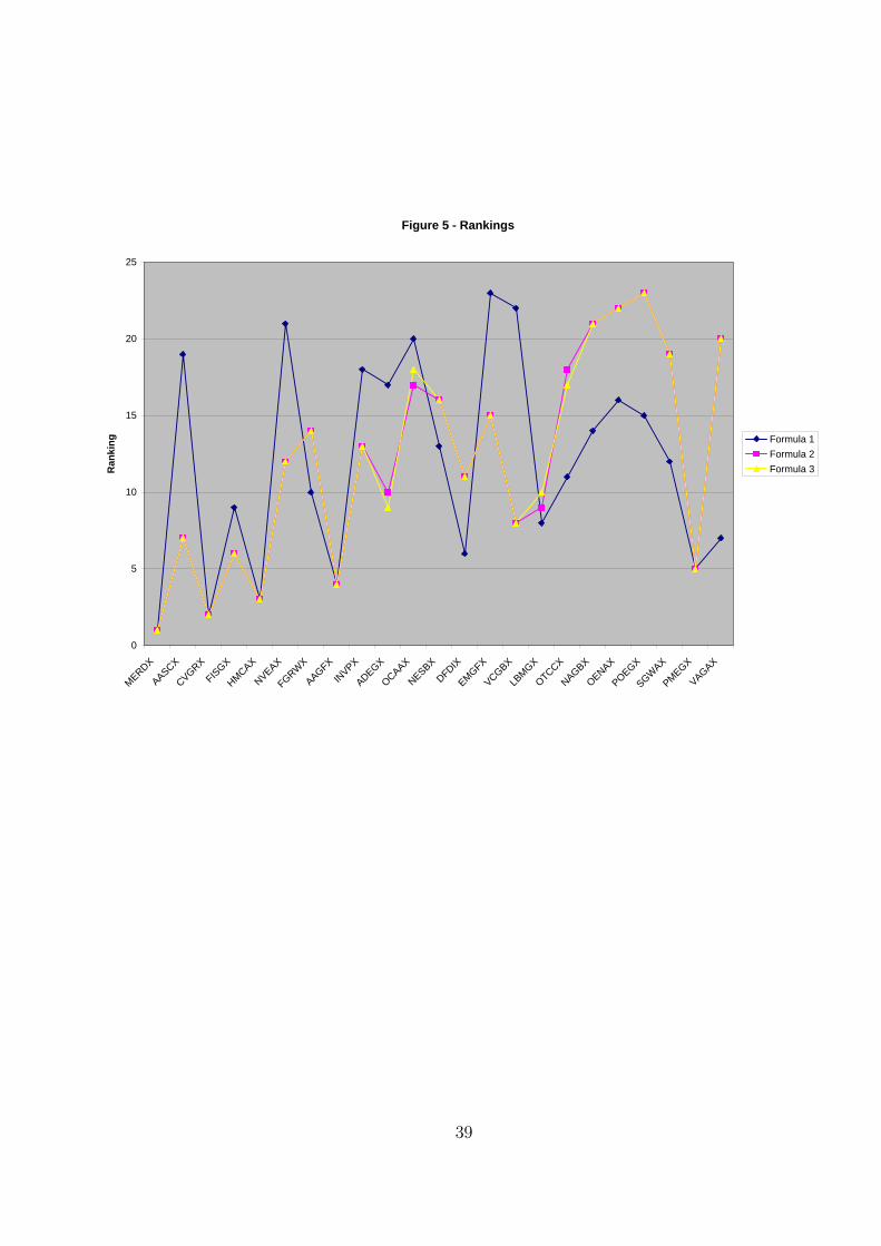
Figure 5 - Rankings

0

5

10

15

20

25

MERDX

AASCX

CVGRX

FISGX

HMCAX

NVEAX

FGRWX

AAGFX

INVPX

ADEGX

OCAAX

NESBX

DFDIX

EMGFX

VCGBX

LBM

GX

OTCCX

NAGBX

OENAX

POEGX

SGWAX

PMEGX

VAGAX

Ran

kin

g Formula 1

Formula 2

Formula 3

39

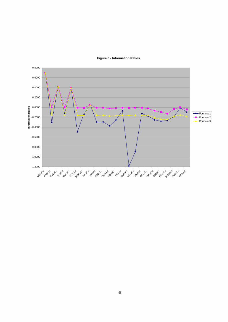
Figure 6 - Information Ratios

-1.2000

-1.0000

-0.8000

-0.6000

-0.4000

-0.2000

0.0000

0.2000

0.4000

0.6000

0.8000

MERDX

AASCX

CVGRX

FISGX

HMCAX

NVEAX

FGRWX

AAGFX

INVPX

ADEGX

OCAAX

NESBX

DFDIX

EMGFX

VCGBX

LBM

GX

OTCCX

NAGBX

OENAX

POEGX

SGWAX

PMEGX

VAGAX

Info

rmat

ion

Rat

ios

Formula 1

Formula 2

Formula 3

40

D References

References

[1] The Brandes Institute “The ’Misinformation’ Ratio: Manipulating Portfolio Risk

Statistics,” Brandes Institute (Sept. 2002): pp. 1-2.

[2] Clarke, R. G., de Silva, H., and Wander, B., “Risk Allocation Versus Asset Allo-

cation,” Journal of Portfolio Management 29 (Fall 2002): pp. 1-6.

[3] Elton, Gruber, Brown, and Goetzmann. Modern Portfolio Theory and Investment

Analysis, Sixth Edition. New York: John Wiley & Sons, Inc., 2003

[4] Goodwin, Thomas H. “The Information Ratio,” Financial Analysts Journal 54

(July/Aug 1998): pp. 1-10.

[5] Grinold, Richard C. “Alpha is Volatility Times IC Times Score,” Journal of Port-

folio Management 20 (Summer 1994): pp. 1-8.

[6] Grinold, Richard C. and Kahn, Ronald N. Active Portfolio Management, New

York: McCraw-Hill, 2000.

[7] Grinold, Richard C. and Kahn, Ronald N. “Information Analysis,” Journal of

Portfolio Management 18 (Spring 1992): pp. 1-8.

[8] Gupta, Prajogi, and Stubbs, “The Information Ratio and Performance,” Journal

of Portfolio Management 26 (Fall 1999): pp. 1-8.

[9] Israelsen, Craig L. “The IR Repair Kit,” Financial Planning Magazine (May

2004): pp. 1-4.

[10] Kahn, Ronald N. “Bond Manager Need To Take More Risk,” Journal of Portfolio

Management 24 (Spring 1998): pp. 1-9.

41

[11] Markowitz, H.M. (1952) “Portfolio Selection,” Journal of Finance, 7(1), March,

pp. 77-91.

[12] Markowitz, H.M. (1987) Mean-Variance Analysis in Portfolio Choice and Capital

Markets, Faboozi and Associates

[13] Muralidhar, Arun S. “Risk-adjusted performance: The correlation correction,”

Financial Analysts Journal 56 (Sep/Oct 2000): pp. 1-11.

[14] Schmidt, Finneran, and Armstrong. “Manipulating Portfolio Risk Statistics,” Pen-

sions & Investments 30 (Sept. 2002): pp. 1-3.

[15] Sharpe, William F. “The Sharpe Ratio,” Journal of Portfolio Management 21

(1994): pp. 1-15.

[16] Thomas III, Lee R. “Active Management,” Journal of Portfolio Management 26

(Winter 2000): pp. 1-11.

42