an improved sharp interface method for viscoelastic and...
TRANSCRIPT
J Sci ComputDOI 10.1007/s10915-007-9173-5
An Improved Sharp Interface Method for Viscoelasticand Viscous Two-Phase Flows
P.A. Stewart · N. Lay · M. Sussman · M. Ohta
Received: 20 February 2007 / Revised: 9 October 2007 / Accepted: 5 November 2007© Springer Science+Business Media, LLC 2007
Abstract We introduce a robust method for computing viscous and viscoelastic two-phasebubble and drop motions. Our method utilizes a coupled level-set and volume-of-fluid tech-nique for updating and representing the air-water interface. Our method introduces a novelapproach for treating the viscous coupling terms at the air-water interface; these improve-ments result in improved stability for computing two-phase bubble formation solutions. Wealso present an improved, “positive-preserving” discretization technique for updating theconfiguration tensor for viscoelastic flows, in the context of computing two-phase bubbleand drop motion.
Keywords Level-set method · Volume-of-fluid method · Two-phase flow · Bubbles · Drops
1 Introduction
In [1, 2], and [3], a sharp interface method was developed for computing solutions to prob-lems in Newtonian two-phase flows and viscoelastic two-phase flows. The interface separat-ing the two phases in these papers was represented and updated using the coupled level setand volume-of-fluid method. The treatment of interfacial boundary conditions for our sharpinterface method has the property that in the limit of zero gas density and zero gas viscosity,i.e. in the limit that the gas is treated as a zero density void, the solutions approach the so-lutions of the corresponding one-phase problem. The air-water interface for the one-phaseproblem is a free-surface in which the liquid on one side is treated as an incompressible fluidand the gas pressure on the other side of the free-surface is treated as spatially constant.
P.A. Stewart · N. Lay · M. Sussman (�)Department of Mathematics, Florida State University, Tallahassee, FL 32306, USAe-mail: [email protected]
M. OhtaDepartment of Applied Chemistry, Muroran Institute of Technology, 27-1, Mizumotocho, Muroran-shi,Hokkaido 050-8585, Japane-mail: [email protected]
J Sci Comput
We remark that Kang et al. [4] used the Ghost Fluid Method [5] and techniques in [6] totreat multiphase incompressible flow, including the effects of viscosity, surface tension, andgravity using a sharp interface method. Their method takes the interfacial jump conditionsinto consideration, but they use an explicit formulation of viscous terms. References [1–3], and this paper utilize an implicit treatment of the viscous terms. Our treatment takesthe location of the interface into consideration and uses the knowledge that the two-phasealgorithm reduces to a one-phase algorithm in the limit that gas becomes a constant pressurevoid.
In this paper we present two improvements, in the context of our sharp interface method;(1) we present improvements for the discretization of the “coupling” terms that appear inthe viscous force terms and (2) we present improved discretization techniques for updatingthe configuration tensor for viscoelastic flows.
1.1 Improvements in Calculating the Viscous Force Terms
We introduce a robust method for computing viscosity in two-phase bubble and drop mo-tions. Sussman et al. [1] described a sharp interface method for incompressible two-phaseflows. This method uses a coupled level-set and volume-of-fluid technique for updating andrepresenting the air-water interface, and introduces a novel approach for treating the jumpconditions at the air-water interface. This method yielded solutions in the zero gas densitylimit which were comparable in accuracy to the method in which the gas pressure was treatedas spatially constant. This improvement allowed for increases in the accuracy of solutionson coarse grids.
However, the above method’s matrix solver would not converge when viscous effectswere dominant. The above method also was inefficient in the sense that it used a secondorder time discretization, even though the spatial error in discretizing the viscous force termswas only first order accurate. Li et al. [7] gave a method to decouple problematic viscousterms with a low Reynolds number. This provided a basis for Sussman and Ohta to describeimprovements for calculating two-phase bubble and drop motions [3].
The new method proposed by Sussman-Ohta [3] no longer suffered from problems withlarge viscous terms. The decoupling of the viscous terms resulted in a diagonally dominantmatrix system for the non-coupled viscous force terms; such a matrix system could be ro-bustly solved using the conjugate gradient method or multigrid method. This new methodinvolved a first order, backwards Euler time discretization for the non-coupled viscous termsand was comparably better than [1] when viscous effects are dominant.
However, the calculation of the viscous coefficients used for the coupling terms in [3]are not as accurate as they could be, and the method will lead to instabilities in some calcu-lations. The analysis done in [7] only considered the temporal discretization when provingunconditional stability for their method. We show through example in this paper that thesemi-implicit approach taken by [3] works well for many bubble and drop two-phase flowproblems, but fails for the bubble formation problem for certain parameter regimes. Here,we shall introduce a new method to improve the evaluations of the viscous coupling-termcoefficients. Our method does not lead to instabilities and is either just as accurate as themethods proposed in [1] and [3], or for some problems, measurably more accurate.
Other methods of interest include [8] and [9]. In [8], Hong et al. treats their viscousterms implicitly in a method similar to that described in [3]. However, they assume that thenet result of their viscous coupling terms is zero. In [9], Rasmussen et al. also use a methodsimilar to that described in [3]. However, their method for discretizing the viscous forceterms is developed in the context of one-phase flow with variable liquid viscosity, instead
J Sci Comput
of two-phase flow; we focus on the treatment of the viscous force terms at a two-phaseinterface where both density and viscosity have large jumps.
1.2 A Positive Definite Preserving Numerical Scheme for Updating the ConfigurationTensor for Viscoelastic Two-Phase Flow
Algorithms for viscoelastic two-phase flow have been presented by Yu et al. [10], Pilla-pakkam and Singh [11], and Jimenez et al. [2]. Also, algorithms for viscoelastic one-phaseflow have been presented by Goktekin et al. [12], Losasso et al. [13] and Irving [14]. We re-mark that the previous methods [10] and [11] were developed in the context of a “smoothed”interface method, instead of the sharp interface method presented here. The work by [12–14]was developed in the context of a one-phase flow algorithm in which the gas pressure wasassumed spatially constant. We note that, as remarked by Losasso et al. [13], Goktekin etal. [12] ignored the fluid rotation term since Goktekin et al. solved the following simplifiedequation for the elastic strain tensor ε:
εt + �u · ε = (∇�u + (∇�u)T )/2 − εPlastict .
In this paper, we describe improvements to the work presented by Jimenez et al. [2] for thediscretization of the evolution equation for the configuration tensor A:
∂A∂t
+ u · ∇A = A · (∇u)T + ∇u · A − f (R)
λ(A − I). (1.1)
For the FENE–CR model [15], the conformation of the polymer is specified in terms of theaverage of the dyadic product 〈RR〉 of the dumbbell end-to-end vector R. c,L,λ are FENE–CR model parameters. The parameter c is a measure of the concentration of dumbbells, L isthe extensibility parameter which denotes the maximum average length of s polymer mole-cule relative to the equilibrium end-to-end dimension, λ is a characteristic relaxation time.The FENE–CR model has a constant shear viscosity and the FENE–CR model reduces tothe Oldroyd-B model as L → ∞. The function f (R) specifies the nonlinear spring charac-teristics of the viscoelastic fluid and is given by
f (R) = 1
1 − tr(A)/L2. (1.2)
In particular, we observe that (1.1) preserves A as a positive definite matrix. The discretiza-tion of (1.1) should preserve the positive definite property of A as well. In our previouswork [2], we only preserved the diagonal entries of A to be positive. We remark that thereare many choices of schemes for discretizing (1.1), see e.g. [16, 17] and [18], but they arecomplicated, and ultimately one must reduce the order of accuracy of a method to first orderin order to preserve positive definiteness of A. We instead base our discretization on thefollowing observation that one can rewrite (1.1) as follows,
A(x, t + �t) = I + ((I + �t∇U)A(x − U�t, t)(I + �t∇U)T − I )e−f (R)
λ�t + O(�t2).
(1.3)We show that we can robustly calculate viscoelastic bubbly flows using our new method
for updating the configuration tensor together with our sharp interface approach.We remark that a similar “matrix transformation” technique as given in (1.3) was also
implemented by [14]. I.e., [14] also implemented a semi-Lagrangian advection step to

J Sci Comput
find ε(x − U�t, t) and then computed the similarity transformation SεST where S =12 (∇U − ∇UT ). The viscoelastic model in [14] was based on the corotational Maxwellmodel and the viscoelastic model in this paper is based on the FENE–CR model. The nu-merical discretization in [14] does not preserve the positive definite property of their elasticstrain tensor, whereas our numerical discretization does preserve the configuration tensor,A, as a positive definite matrix.
2 Governing Equations
The governing equations for incompressible, immiscible two-phase flow was written byChang et al. [19] as:
ρDU
Dt= ∇·
(−pI + 2μD + ηP
λf (R)A
)+ ρgz − σκ(F )∇H,
∂A∂t
+ U · ∇A = A · (∇U)T + ∇U · A − f (R)
λ(A − I),
(2.1)∇ · U = 0,
Dφ
Dt= 0,
DF
Dt= 0,
ρ = ρLH(φ) + ρG(1 − H(φ)), μ = μLH(φ) + μG(1 − H(φ)), ηP = ηP H(φ),
H(φ) ={
1, φ ≥ 0,
0, φ < 0,
φ is a level set function which is positive in liquid and negative in gas. F is a volume-of-fluidfunction which represents the fraction of fluid that is liquid for each computational cell. Ourmethod follows the time-splitting that was used in Sussman and Ohta [3] for decoupling theviscous terms, and also uses the previously developed CLSVOF method by Sussman andPuckett [20] by coupling the solutions of φ and F .
Other variables used are defined as: U is the velocity field, p is the pressure, D =12 (∇U + ∇UT ) is the rate of deformation tensor, g corresponds to the acceleration dueto gravity, μL(μG) is the viscosity of liquid (gas), ρL(ρG) is the density of liquid (gas),κ(F ) = ∇ · ∇F
|∇F | is the curvature, and σ is the coefficient of surface tension. The gradientterms on the right hand side of the equation for A are defined as
A · (∇U)T + ∇U · A = Aαγ
∂Uβ
∂xγ
+ ∂Uα
∂xγ
Aγβ .
3 Viscosity: An Adaptive, Sharp Interface Treatment for the Viscous Force Terms
We present a simple and robust adaptive method for computing the viscous forces as theyappear in (2.1),
∇ · (2μD). (3.1)
J Sci Comput
Our algorithm follows the same strategy as proposed by Li, Renardy, and Renardy [7] andas implemented in Sussman-Ohta [3] by discretizing the coupling terms in (3.1) explicitlyand the remainder of the terms implicitly. It was shown by Li et al. [7] that the followingtemporal discretization for the viscous forces is stable for any time step:
ρu∗∗ − u∗
�t= ∇ · μ∇u∗∗ + (
μu∗∗x
)x+ (
μν∗x
)y+ (
μw∗x
)z,
ρν∗∗ − ν∗
�t= ∇ · μ∇ν∗∗ + (
μν∗∗y
)y+ (
μu∗y
)x+ (
μw∗y
)z,
ρw∗∗ − w∗
�t= ∇ · μ∇w∗∗ + (
μw∗∗z
)z+ (
μu∗z
)x+ (
μν∗z
)y.
The non-coupling terms are discretized using standard finite volume techniques. For exam-ple, we approximate the terms ∇ · μ∇u∗∗ + (μu∗∗
x )x from above as,
2μi+1/2,j,k(ui+1,j,k − ui,j,k) − 2μi−1/2,j,k(ui,j,k − ui−1,j,k)
�x2
+μi,j+1/2,k(ui,j+1,k − ui,j,k) − μi,j−1/2,k(ui,j,k − ui,j−1,k)
�y2
+μi,j,k+1/2(ui,j,k+1 − ui,j,k) − μi,j,k−1/2(ui,j,k − ui,j,k−1)
�z2.
The face centered viscosity, μi+1/2,j,, is defined “sharply” as,
μi+1/2,j, = 1θi+1/2,j
μL+ 1−θi+1/2,j
μG
.
θi+1/2,j is the height fraction [7, 8] given by:
θi+1/2,j (φ) =
⎧⎪⎪⎪⎨⎪⎪⎪⎩
1, φi+1,j , φi,j ≥ 0,
0, φi+1,j , φi,j < 0,
φ+i+1,j + φ+
i,j
|φi+1,j | + |φi,j | , otherwise.
(3.2)
The “+” superscript stands for the positive part, i.e. a+ ≡ max(a,0). The combined densityis also defined sharply as,
H(ρ) ={
ρL, φ ≥ 0,
ρG, φ < 0.
In Sussman and Ohta [3], the coupling terms were discretized in two dimensions as
∂(μνx)
∂y≈ (
μi+1/2,j+1/2(νx)i+1/2,j+1/2 − μi+1/2,j−1/2(νx)i+1/2,j−1/2
+μi−1/2,j+1/2(νx)i−1/2,j+1/2 − μi−1/2,j−1/2(νx)i−1/2,j−1/2)/2�y,
∂(μuy)
∂x≈ (
μi+1/2,j+1/2(uy)i+1/2,j+1/2 − μi−1/2,j+1/2(uy)i−1/2,j+1/2
+μi+1/2,j−1/2(uy)i+1/2,j−1/2 − μi−1/2,j−1/2(uy)i−1/2,j−1/2)/2�x.
J Sci Comput
The viscosity at a node was given by
μi+1/2,j+1/2 =
⎧⎪⎪⎪⎨⎪⎪⎪⎩
μL, θi+1/2,j+1/2 = 1,
μG, θi+1/2,j+1/2 = 0,
0, μG = 0 and 0 < θi+1/2,j+1/2 < 1,
μLG, otherwise,
where
μLG = μGμL
μGθi+1/2,j+1/2 + μL(1 − θi+1/2,j+1/2).
θi+1/2,j+1/2 is a “node fraction” defined as,
θi+1/2,j+1/2(ϕ) =
⎧⎪⎨⎪⎩
1, φi+1,j , φi,j , φi,j+1, φi+1,j+1 ≥ 0,
0, φi+1,j , φi,j , φi,j+1, φi+1,j+1 < 0,
θND, otherwise.
The “+” superscript stands for the positive part, i.e. a+ ≡ max(a,0), and
θND = φ+i+1,j + φ+
i,j+1 + φ+i,j + φ+
i+1,j+1
|φi+1,j | + |φi,j+1| + |φi,j | + |φi+1,j+1| .
The components of the parts of the deformation tensor that are handled explicitly, e.g. thecoupled terms, (uy)i+1/2,j+1/2 in the equation for ν and (νx)i+1/2,j+1/2 in the equations foru, were calculated at nodes using standard central differencing, i.e.,
(uy)i+1/2,j+1/2 = ui+1,j+1 − ui+1,j + ui,j+1 − ui,j
2�y.
The discretization of the viscous terms in [3] had the following properties:
1. If the gas viscosity is zero, the velocity in gas cells, ϕi,j < 0, is never used. This enabledour two-phase method to be equivalent to the corresponding one-phase method in thelimit of zero gas density and zero gas viscosity (i.e. gas treated as vacuum with uniformpressure).
2. The resulting matrix system for each velocity component is written in the following form,
α(x)p + β∇ · (A(x, y)∇p) = f (x, y). (3.3)
Where (3.3) is solved for p. A is a diagonal matrix. Reference [3] solved (3.3) on anadaptive hierarchy of grids as also described in Sect. 5.
In this paper, we discretize the coupling terms differently from [3]; in three dimensions,they appear as:
∂u
∂y
∣∣∣∣i−1/2,j,k
= ωi,j,k
i,j+1,k(ui,j+1,k − ui,j,k) + ωi,j−1,k
i,j,k (ui,j,k − ui,j−1,k)
�y(ωi,j,k
i,j+1,k + ωi,j−1,k
i,j,k + ωi−1,j,k
i−1,j+1,k + ωi−1,j−1,k
i−1,j,k )
+ωi−1,j,k
i−1,j+1,k(ui−1,j+1,k − ui−1,j,k) + ωi−1,j−1,k
i−1,j,k (ui−1,j,k − ui−1,j−1,k)
�y(ωi,j,k
i,j+1,k + ωi,j−1,k
i,j,k + ωi−1,j,k
i−1,j+1,k + ωi−1,j−1,k
i−1,j,k ),

J Sci Comput
∂u
∂z
∣∣∣∣i−1/2,j,k
= ωi,j,k
i,j,k+1(ui,j,k+1 − ui,j,k) + ωi,j,k−1i,j,k (ui,j,k − ui,j,k−1)
�z(ωi,j,k
i,j,k+1 + ωi,j,k−1i,j,k + ω
i−1,j,k
i−1,j,k+1 + ωi−1,j,k−1i−1,j,k )
+ωi−1,j,k
i−1,j,k+1(ui−1,j,k+1 − ui−1,j,k) + ωi−1,j,k−1i−1,j,k (ui−1,j,k − ui−1,j,k−1)
�z(ωi,j,k
i,j,k+1 + ωi,j,k−1i,j,k + ω
i−1,j,k
i−1,j,k+1 + ωi−1,j,k−1i−1,j,k )
,
where,
ωL,M,NI,J,K =
{1, sφI,J,K ≥ 0 and sφL,M,N ≥ 0,
0, otherwiseand
s ={
1, φi−1,j,k ≥ 0 or φi,j,k ≥ 0,
−1, otherwise,
∂ν
∂x
∣∣∣∣i,j−1/2,k
= ωi,j,k
i+1,j,k(νi+1,j,k − νi,j,k) + ωi−1,j,k
i,j,k (νi,j,k − νi−1,j,k)
�x(ωi,j,k
i+1,j,k + ωi−1,j,k
i,j,k + ωi,j−1,k
i+1,j−1,k + ωi−1,j−1,k
i,j−1,k )
+ωi,j−1,k
i+1,j−1,k(νi+1,j−1,k − νi,j−1,k) + ωi−1,j−1,k
i,j−1,k (νi,j−1,k − νi−1,j−1,k)
�x(ωi,j,k
i+1,j,k + ωi−1,j,k
i,j,k + ωi,j−1,k
i+1,j−1,k + ωi−1,j−1,k
i,j−1,k ),
∂ν
∂z
∣∣∣∣i,j−1/2,k
= ωi,j,k
i,j,k+1(νi,j,k+1 − νi,j,k) + ωi,j,k−1i,j,k (νi,j,k − νi,j,k−1)
�z(ωi,j,k
i,j,k+1 + ωi,j,k−1i,j,k + ω
i,j−1,k
i,j−1,k+1 + ωi,j−1,k−1i,j−1,k )
+ωi,j−1,k
i,j−1,k+1(νi,j−1,k+1 − νi,j−1,k) + ωi,j−1,k−1i,j−1,k (νi,j−1,k − νi,j−1,k−1)
�z(ωi,j,k
i,j,k+1 + ωi,j,k−1i,j,k + ω
i,j−1,k
i,j−1,k+1 + ωi,j−1,k−1i,j−1,k )
,
where,
ωL,M,NI,J,K =
{1, sφI,J,K ≥ 0 and sφL,M,N ≥ 0,
0, otherwiseand
s ={
1, φi,j−1,k ≥ 0 or φi,j,k ≥ 0,
−1, otherwise,
∂w
∂x
∣∣∣∣i,j,k−1/2
= ωi,j,k
i+1,j,k(wi+1,j,k − wi,j,k) + ωi−1,j,k
i,j,k (wi,j,k − wi−1,j,k)
�x(ωi,j,k
i+1,j,k + ωi−1,j,k
i,j,k + ωi,j,k−1i+1,j,k−1 + ω
i−1,j,k−1i,j,k−1 )
+ωi,j,k−1i+1,j,k−1(wi+1,j,k−1 − wi,j,k−1) + ω
i−1,j,k−1i,j,k−1 (wi,j,k−1 − wi−1,j,k−1)
�x(ωi,j,k
i+1,j,k + ωi−1,j,k
i,j,k + ωi,j,k−1i+1,j,k−1 + ω
i−1,j,k−1i,j,k−1 )
,
∂w
∂y
∣∣∣∣i,j,k−1/2
= ωi,j,k
i,j+1,k(wi,j+1,k − wi,j,k) + ωi,j−1,k
i,j,k (wi,j,k − wi,j−1,k)
�y(ωi,j,k
i,j+1,k + ωi,j−1,k
i,j,k + ωi,j,k−1i,j+1,k−1 + ω
i,j−1,k−1i,j,k−1 )
+ωi,j,k−1i,j+1,k−1(wi,j+1,k−1 − wi,j,k−1) + ω
i,j−1,k−1i,j,k−1 (wi,j,k−1 − wi,j−1,k−1)
�y(ωi,j,k
i,j+1,k + ωi,j−1,k
i,j,k + ωi,j,k−1i,j+1,k−1 + ω
i,j−1,k−1i,j,k−1 )
,

J Sci Comput
where,
ωL,M,NI,J,K =
{1, sφI,J,K ≥ 0 and sφL,M,N ≥ 0,
0, otherwiseand
s ={
1, φi,j,k−1 ≥ 0 or φi,j,k ≥ 0,
−1, otherwise.
We may now write the viscous coupling terms as
∂(μ∂u
∂y
)∂x
∣∣∣∣i,j,k
≈μi+1/2,j,k
∂u∂y
∣∣i+1/2,j,k
− μi−1/2,j,k∂u∂y
∣∣i−1/2,j,k
�x,
∂(μ∂u
∂z
)∂x
∣∣∣∣i,j,k
≈μi+1/2,j,k
∂u∂z
∣∣i+1/2,j,k
− μi−1/2,j,k∂u∂z
∣∣i−1/2,j,k
�x,
∂(μ∂ν
∂x
)∂y
∣∣∣∣i,j,k
≈μi,j+1/2,k
∂ν∂x
∣∣i,j+1/2,k
− μi,j−1/2,k∂ν∂x
∣∣i,j−1/2,k
�y,
∂(μ∂ν
∂z
)∂y
∣∣∣∣i,j,k
≈μi,j+1/2,k
∂ν∂z
∣∣i,j+1/2,k
− μi,j−1/2,k∂ν∂z
∣∣i,j−1/2,k
�y,
∂(μ∂w
∂x
)∂z
∣∣∣∣i,j,k
≈μi,j,k+1/2
∂w∂x
∣∣i,j,k+1/2
− μi,j,k−1/2∂w∂x
∣∣i,j,k−1/2
�z,
∂(μ∂w
∂y
)∂z
∣∣∣∣i,j,k
≈μi,j,k+1/2
∂w∂y
∣∣i,j,k+1/2
− μi,j,k−1/2∂w∂y
∣∣i,j,k−1/2
�z.
3.1 Justification for New Method for Discretizing the Viscous Coupling Terms
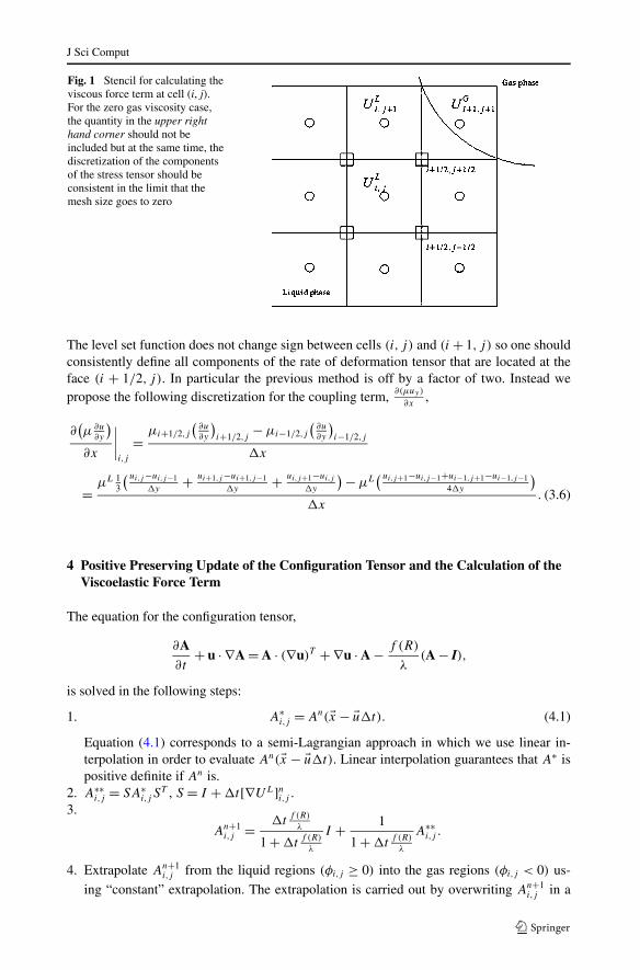
In Sussman and Ohta [3] the discretization of the coupling terms was done in a manner sothat the gas velocity would not be included in the discretization of the viscous force termsin the case μG = 0. This restriction sacrificed consistency in the discretization of the cou-pling terms near the interface. We believe that this inconsistency is the reason why we haveencountered instability for some problems when treating the coupling terms explicitly. Inorder to illustrate the problem, and in order to illuminate the reasoning behind our solution,we refer the reader to Fig. 1. If we were to implement the method described by Sussman andOhta [3], one would define the following nodal viscosities:
μi+1/2,j+1/2 = 0, μi+1/2,j−1/2 = μL.
The resulting discretization for the following coupling term ∂(μuy)
∂xwould be,
(∂(μuy)
∂x
)≈ (
μi+1/2,j−1/2(uy)i+1/2,j−1/2 + (0)(uy)i+1/2,j+1/2
−μi−1/2,j−1/2(uy)i−1/2,j−1/2 − μi−1/2,j+1/2(uy)i−1/2,j+1/2
)/2�x. (3.4)
The first two terms of (3.4) combines to be an inconsistent discretization of the quantity,
μL
(∂u
∂y
)i+1/2,j
. (3.5)
J Sci Comput
Fig. 1 Stencil for calculating theviscous force term at cell (i, j).For the zero gas viscosity case,the quantity in the upper righthand corner should not beincluded but at the same time, thediscretization of the componentsof the stress tensor should beconsistent in the limit that themesh size goes to zero
The level set function does not change sign between cells (i, j) and (i + 1, j) so one shouldconsistently define all components of the rate of deformation tensor that are located at theface (i + 1/2, j). In particular the previous method is off by a factor of two. Instead wepropose the following discretization for the coupling term, ∂(μuy)
∂x,
∂(μ∂u
∂y
)∂x
∣∣∣∣i,j
=μi+1/2,j
(∂u∂y
)i+1/2,j
− μi−1/2,j
(∂u∂y
)i−1/2,j
�x
= μL 13
( ui,j −ui,j−1�y
+ ui+1,j −ui+1,j−1�y
+ ui,j+1−ui,j
�y
) − μL( ui,j+1−ui,j−1+ui−1,j+1−ui−1,j−1
4�y
)�x
. (3.6)
4 Positive Preserving Update of the Configuration Tensor and the Calculation of theViscoelastic Force Term
The equation for the configuration tensor,
∂A∂t
+ u · ∇A = A · (∇u)T + ∇u · A − f (R)
λ(A − I),
is solved in the following steps:
1. A∗i,j = An(�x − �u�t). (4.1)
Equation (4.1) corresponds to a semi-Lagrangian approach in which we use linear in-terpolation in order to evaluate An(�x − �u�t). Linear interpolation guarantees that A∗ ispositive definite if An is.
2. A∗∗i,j = SA∗
i,j ST , S = I + �t[∇UL]ni,j .
3.
An+1i,j = �t
f (R)
λ
1 + �tf (R)
λ
I + 1
1 + �tf (R)
λ
A∗∗i,j .
4. Extrapolate An+1i,j from the liquid regions (φi,j ≥ 0) into the gas regions (φi,j < 0) us-
ing “constant” extrapolation. The extrapolation is carried out by overwriting An+1i,j in a
J Sci Comput
gas cell with the corresponding value from the nearest liquid cell. Constant extrapola-tion guarantees that the extrapolated configuration tensor remains positive definite if theoriginal was positive definite as well.
The viscoelastic force term, ∇ · ( ηP
λf (R)A), is calculated in the following steps:
(a) extrapolate the tensor, Bi,j = ηP
λf (R)i,jAi,j , from cell centers to cell faces. E.g.
Bi+1/2,j = (ηp)i+1/2,j
λ
(f (R)A)i+1,j + (f (R)A)i,j
2, where
(ηP )i+1/2,j ={
ηP , φi+1,j ≥ 0 and φi,j ≥ 0,
0, otherwise.
(b) The components of the viscoelastic force vector are then written as:
(Lviscoelastici,j )γ = (Bi+1/2,j )γ,1 − (Bi−1/2,j )γ,1
�x+ (Bi,j+1/2)γ,2 − (Bi,j−1/2)γ,2
�y.
4.1 Proof of the Positive Definite Preserving Property for the Configuration TensorUpdate Step
Each of the steps one thru four in Sect. 4 above preserves the configuration tensor as apositive definite symmetric matrix. This fact can be proved so long as the following stabilityconstraint is satisfied,
�t <1
2d
�x
max |U | , (4.2)
where d is the dimension of the problem (2 or 3). We first consider step 1 above. Withoutloss of generality, we consider step 1 (4.1) in one dimension with positive velocity u. Thenone has
A∗i = An(x − u�t) = u�t
�xAn
i−1 +(
1 − u�t
�x
)An
i . (4.3)
The stability constraint (4.2) insures that the coefficients of A in (4.3) are positive which inturn insures that A∗ is positive definite symmetric since the linear combination of positivedefinite symmetric matrices, with positive coefficients, is also positive definite symmetric.In step 2 of Sect. 4 above, the stability constraint (4.2) insures that the matrix,
S = I + �t[∇UL]ni,j ,
is nonsingular. Since S is nonsingular, and A∗ is positive definite symmetric, this implies thatthe matrix A∗∗ = SA∗ST is also a positive definite symmetric matrix. In step 3 of Sect. 4above, we have the linear combination of two positive definite symmetric matrices, withpositive coefficients, which insures that An+1 is also positive definite symmetric. Finally,the extrapolation step (step 4) preserves the extrapolated values of An+1 as positive definitesymmetric since we are implementing a piecewise constant extrapolation algorithm. We notethat for our choice of f (R) in (1.2), we have to treat the special case when trace(A) ≥ L2; inthis case we assume a relaxation time of zero and therefore replace the configuration tensorAwith the identity matrix I .

J Sci Comput
5 Matrix Solver
The equations resulting from the calculations of the viscous force terms or the pressureprojection steps can be written generally as,
α(x)p + β∇ · (A(x, y)∇p) = f (x, y) + α(x)q + β∇ · V, (5.1)
where A is a diagonal matrix. We discretize (5.1) as,
αijpijβ(DGp)ij = fij + αij qij + β(DV )ij , (5.2)
where
(Gp)i+1/2,j = (A11)i+1/2,j
pi+1,j − pij
�x, (Gp)i,j+1/2 = (A22)i,j+1/2
pi,j+1 − pij
�y,
(DV )i,j = ui+1/2,j − ui−1/2,j
�x+ νi,j+1/2 − νi,j−1/2
�y.
We solve (5.2) with a combination of the multigrid method and the mutligrid preconditionedconjugate gradient method (MGPCG) [21]. The adaptive composite solver will converge toany specified tolerance ε, as long as we compute the solution on each level (using MGPCG)to a tolerance of ε × 10−2 each time the outer multigrid solver visits a level. Our Multi-grid+MGPCG algorithm for solving (5.2) follows the same “V-cycle” procedure as outlinedby Briggs, et al. [22]:
Put (5.2) in residual correction form:For l = 0 . . . lmax
V l = V l − Gplpredict
ql = ql − plpredict
pl = plpredict
EndFor
Then, call recursive subroutine MV(l):
subroutine MV(l)1. if l < lmax then restrict V l+1 to level l
2. Rl = f l + αql + βDV l
3. if l < lmax then restrict Rl+1 to level l
4. V lsave = V l, ql
save = ql,Rlsave = Rl
5. plcor = 0
6. Iterate until the residual on level l is less than the tolerance ε × 10−2.Iterate using MGPCG,
αplcor + βDGpl
cor = Rlsave
7. Rl = Rlsave − αpl
cor − βDGplcor, V l = V l − Gp1
cor, ql = ql − plcor
8. if l > 0 then
{call MV (l − 1)
prolongate pl−1cor to level l, pl
cor = plcor + I l
l−1pl−1cor
9. Iterate until the residual on level l is less than the tolerance ε × 10−2.Iterate using MGPCG,
αplcor + βDGpl
cor = Rlsave
10. V l = V lsave − Gpl
cor, ql = qlsave − pl
cor, pl = pl + plcor
J Sci Comput
6 Overall Numerical Algorithm for Two-Phase Viscoelastic/Viscous Flow
Prior to each time step, we are given a liquid velocity, UL,n, and a total velocity Un. UL,n
corresponds to Un except on gas faces, where we replace the gas velocity in UL,n with theextrapolated liquid velocity. UL,n is then used to calculate the nonlinear advective terms inthe liquid and also used to advance the free surface.
Prior to each time step, we are also given a level set function, ϕn and a volume-of-fluid function Fn. The level set function and the volume-of-fluid function are stored at cellcenters. The velocity is stored at both cell centers and face-centers.
An outline of our numerical algorithm is as follows:
1. CLSVOF; interface advection [1]:
ϕn+1ij = ϕn
ij − �t[UL · ∇φ]ij , F n+1ij = Fn
ij − �t[UL · ∇F ]ij .2. Calculate (cell centered) advective force terms:
ALij = [UL · ∇UL]nij , Aij = [U · ∇U ]nij .
The nonlinear advective terms are discretized using upwind, second order Van-Leer sloplimiting [1, 23].
3. Update the configuration tensor (viscoelastic flows):
An+1i,j = �t
f (R)
λI + (SAn(�x − �u�t)ST )i,j
1 + �tf (R)
λ
, S = I + �t∇U. (6.1)
Please see Sect. 4 for details that describe the discretization of (6.1).4. Calculate (cell centered) semi-implicit viscous forces and explicit viscoelastic forces:
Uni,j =
{U
L,ni,j , φi,j ≥ 0,
Uni,j , φi,j < 0,
Aij ={
ALi,j , φi,j ≥ 0,
Ai,j , φi,j < 0,
U ∗i,j = Un
i,j + �t(−Ai,j + Lviscoelastici,j + gz),
ρU ∗∗ − U ∗
�t= L∗∗,uncoupled + L∗,uncoupled.
The term L∗∗,uncoupled represents the uncoupled viscous force terms which are handledimplicitly, and the term L∗,coupled represents the coupled viscous force terms which arehandled explicitly.
5. Interpolate cell centered forces to face centered forces and calculate the face centeredsurface tension force:
Vi+1/2,j = Uni+1/2,j + �t
(−Ai+1/2,j + 2
ρi+1,j + ρi,j
(Li+1/2,j + Lviscoelastici+1/2,j )
−[
σκ∇H
ρ
]i+1/2,j
+ gz
).
The Surface tension term,σκi+1/2,j (∇H)i+1/2,j
ρi+1/2,j, is discretized as
σκi+1/2,jH(φi+1,j )−H(φi,j )
ρi+1/2,j �x, where H(φ) =
{1, φ ≥ 0,
0, φ < 0,and
ρi+1/2,j = ρLθi+1/2,j + ρG(1 − θi+1/2,j ).
J Sci Comput
Table 1 Comparison ofcomputational results withanalytical solution for Re � 1
Previous New
Computational Re number 0.0524 0.0524
Analytical solution by Hadamard-Rybczynski 0.0534 0.0534
The discretization of the height fraction θi+1/2,j is described by (3.2). The curvatureκi+1/2,j is computed with second-order accuracy directly from the volume fractions asdescribed in [24] or [1].
6. Implicit pressure projection step:
∇ · ∇p
ρ= ∇ · V, Un+1
i+1/2,j = Vi+1/2,j −[∇p
ρ
]i+1/2,j
.
We solve the resulting linear system using a composite solver for an adaptive hierarchyof grids [25] (see also Sect. 5).
7. Liquid velocity extrapolation; assign UL,n+1i+1/2,j = Un+1
i+1/2,j and then extrapolate UL,n+1i+1/2,j
into the gas region.8. Interpolate face centered velocity to cell centered velocity:
UL,n+1i,j = 1
2
(U
L,n+1i+1/2,j + U
L,n+1i−1/2,j
), Un+1
i,j = 1
2
(Un+1
i+1/2,j + Un+1i−1/2,j
).
7 Results
7.1 Spherical Bubble or Drop with Dominant Viscous Effects and Large Viscosity Jump:Comparison with Analytical and Experimental Results
For a spherical bubble, drop and particle freely moving relative to a fluid of infinite ex-tent with a steady velocity with Re � 1.0, the analytical solution derived by Hadamard-Rybczynsk [26, 27] is well-known as follows:
Re = Eo1.5
6M0.5
(1 + κ
2 + 3κ
). (7.1)
Here, Eo is the Eotvos number, M denotes the Morton number and κ(= μD/μC) is the vis-cosity ratio. Equation (7.1) reduces to Re = Eo1.5
12M0.5 as κ → 0 and becomes Eo1.5
18M0.5 for κ → ∞.We show results for a spherical bubble with low Reynolds number. The computational con-dition is logM = 2.85,Eo = 8.67 which is an experimental condition performed by Bhagaand Weber [28]. Although they examined bubble rise dynamics, in this computation, wechanged to a density ratio λ (= ρD/ρC) = 0.95 and κ = 100 to clearly specify a problemwith a large viscosity jump. The numerical simulations were performed on a 3-d axisym-metric computational domain with a domain length of R = 4D (r-direction) and a domainheight of Z = 6D (z-direction). In the computation, one mesh size on the finest level gridwas set to �x = 0.0104 in terms of the dimensionless bubble/drop diameter (D = 1.0).Comparison of computational results with analytical solution is indicated in Table 1. The er-ror between our computational results and analytical solution is only about 2%. We reiteratethat the fluid properties for this problem exhibit very large viscosity.
J Sci Comput
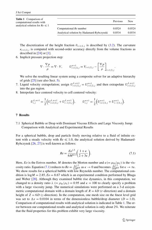
Fig. 2 Left: previous method,right: present method,logM = 2.93, Eo = 116
We then recomputed the previous example (λ = 0.95, κ = 100), except with logM =2.93 and Eo = 116; this test was also performed by Bhaga and Weber [28]. Figure 2 showsa comparison of results using our previous method from [3] and the new methodology de-scribed in this paper. Computational conditions are the same as the case for low Re number.In Fig. 2, the left side is the previous method and the right side corresponds to the newmethod.
7.2 Drop Formation in a Miscible Viscous Liquid
Figure 3 corresponds to the drop formation process in a miscible viscous liquid. Bright [29]injected n-decane into water from a submerged nozzle with d = 1.6 X 10⁻³ m, and he inves-tigated the drop formation process in the system (λ = 0.7327 and κ = 0.90). Richards et al.[30] numerically calculated the Bright’s experimental result on the drop formation processusing the SOLA-VOF method [31] with the continuum surface force (CFS) model [32].In their computation, Richards et al. [30] used the value of the interfacial tension experi-mentally estimated by Johnson and Dettre [33] instead of the interfacial tension measuredby Bright [29]. Our computational conditions for the physical properties follow the paper ofRichards et al. [30]. The computations were carried out in a 3-d axisymmetric computationaldomain with a domain length of R = 16d (r-direction) and a domain height of Z = 32d (z-direction). Also, one mesh size on the finest level grid was �x = 0.0125 in terms of thedimensionless diameter of nozzle (= 1.0). In Fig. 3, the left side is the previous method [3]and the right side corresponds to the new method. We have confirmed that the appearanceof the drop formation reproduced numerically agrees with the experimental result.
7.3 Bubble Formation; Injection of High Speed Gas into Liquid
In test problems with fluids that have a large viscosity, such as the test problem describedin Sect. 7.1 above, a fully implicit treatment of the coupled viscous terms would lead to
J Sci Comput
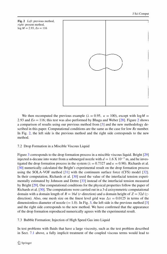
Fig. 3 Drop formation in aviscous liquid. Left: old method,right: new method
Table 2 Grid resolution study for bubble formation problem. Relative errors are displayed. Inflow velocityis 0.9 m/s; density ratio = 1015, viscosity ratio = 70000
Eff. Grid Resolution 64 × 128 128 × 256 256 × 512
Interface Error 0.74 0.45
Gas Velocity Error 1.44 0.65
a matrix system that could not be solved via a standard matrix iterative approach. On theother hand we have found that, for the bubble formation problem, the explicit treatment ofthe viscous coupling terms, as described by [3], leads to instabilities. Here, we perform agrid refinement study using our new approach for a problem that we had previously failed tocompute using the approach described in [3]. The physical properties of the system, togetherwith the inflow velocity condition, are given by the following dimensionless quantities,
ReG = ρGV d
μG
= 99.2, WeG = ρGV 2d
σ= 0.024, Fr = V 2
gd= 46.6,
ρL
ρG
= 1015,μL
μG
= 70000.
The relative errors in Table 1 indicate that we have first order convergence for this problemusing our new treatment for the viscous coupling terms.
J Sci Comput
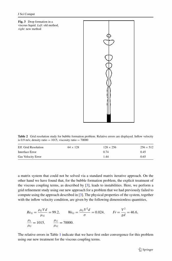
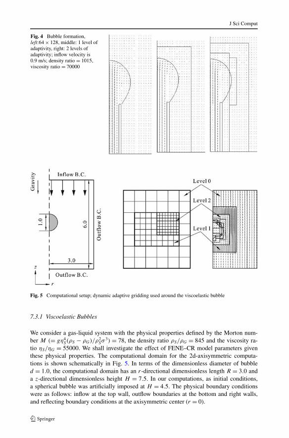
Fig. 4 Bubble formation,left:64 × 128, middle: 1 level ofadaptivity, right: 2 levels ofadaptivity; inflow velocity is0.9 m/s; density ratio = 1015,viscosity ratio = 70000
Fig. 5 Computational setup; dynamic adaptive gridding used around the viscoelastic bubble
7.3.1 Viscoelastic Bubbles
We consider a gas-liquid system with the physical properties defined by the Morton num-ber M (= gη4
S(ρS − ρG)/ρ2Sσ
3) = 78, the density ratio ρS/ρG = 845 and the viscosity ra-tio ηS/ηG = 55000. We shall investigate the effect of FENE–CR model parameters giventhese physical properties. The computational domain for the 2d-axisymmetric computa-tions is shown schematically in Fig. 5. In terms of the dimensionless diameter of bubbled = 1.0, the computational domain has an r-directional dimensionless length R = 3.0 anda z-directional dimensionless height H = 7.5. In our computations, as initial conditions,a spherical bubble was artificially imposed at H = 4.5. The physical boundary conditionswere as follows: inflow at the top wall, outflow boundaries at the bottom and right walls,and reflecting boundary conditions at the axisymmetric center (r = 0).
J Sci Comput
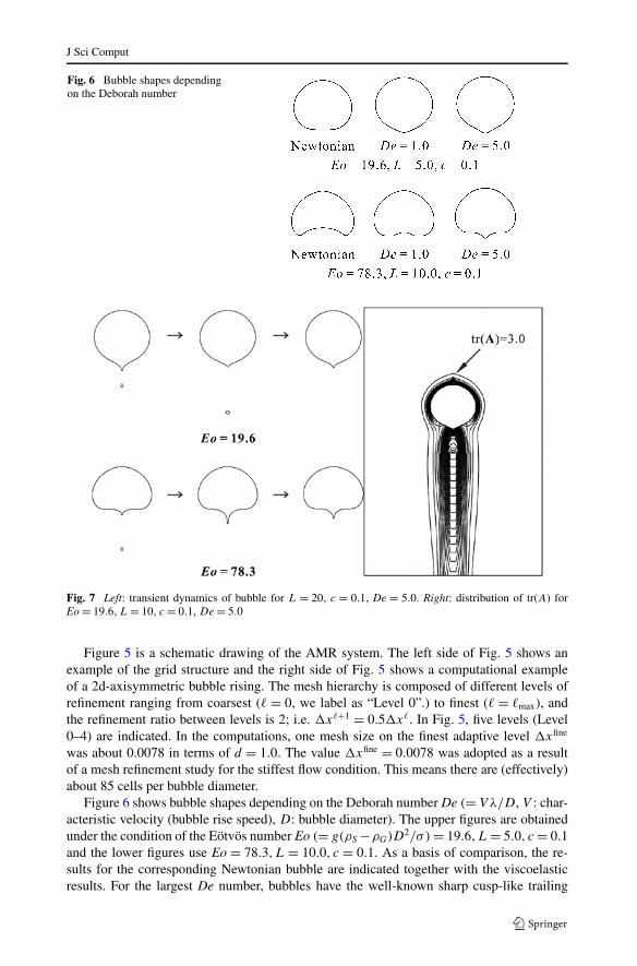
Fig. 6 Bubble shapes dependingon the Deborah number
Fig. 7 Left: transient dynamics of bubble for L = 20, c = 0.1, De = 5.0. Right: distribution of tr(A) forEo = 19.6, L = 10, c = 0.1, De = 5.0
Figure 5 is a schematic drawing of the AMR system. The left side of Fig. 5 shows anexample of the grid structure and the right side of Fig. 5 shows a computational exampleof a 2d-axisymmetric bubble rising. The mesh hierarchy is composed of different levels ofrefinement ranging from coarsest (� = 0, we label as “Level 0”.) to finest (� = �max), andthe refinement ratio between levels is 2; i.e. �x�+1 = 0.5�x�. In Fig. 5, five levels (Level0–4) are indicated. In the computations, one mesh size on the finest adaptive level �xfine
was about 0.0078 in terms of d = 1.0. The value �xfine = 0.0078 was adopted as a resultof a mesh refinement study for the stiffest flow condition. This means there are (effectively)about 85 cells per bubble diameter.
Figure 6 shows bubble shapes depending on the Deborah number De (= V λ/D, V : char-acteristic velocity (bubble rise speed), D: bubble diameter). The upper figures are obtainedunder the condition of the Eötvös number Eo (= g(ρS −ρG)D2/σ) = 19.6, L = 5.0, c = 0.1and the lower figures use Eo = 78.3,L = 10.0, c = 0.1. As a basis of comparison, the re-sults for the corresponding Newtonian bubble are indicated together with the viscoelasticresults. For the largest De number, bubbles have the well-known sharp cusp-like trailing
J Sci Comput
edge. Especially, regardless of the largely dimpled Newtonian bubble for Eo = 78.3, it issurprising that the bubble for L = 10.0, c = 0.1,De = 5.0 has a very long sharp cusp. Thisresult indicates that our computational method can capture largely deformed shapes havinglarge curvature. It is verified that viscoelastic effects (cusp shape) emerge notably as the Denumber becomes larger. Noh et al. [34] gave good physical explanations about the effect ofthe parameters of the FENE–CR model, and our results support their observations. Figure 7shows transient dynamics of bubble motion for the condition of L = 20, c = 0.1,De = 5.0.In this case, the bubble trailing edge is pulled out due to the strong viscoelastic effect (vis-coelastic stress). Consequently, the pulling motion leads to the local breakup of the bubble atthe trailing edge. As an example of the tr(A) profile, the distribution of tr(A) for Eo = 19.6,L = 10, c = 0.1,De = 5.0 is shown as well in Fig. 7. tr(A) is a measure of the degree ofpolymer extension. In Fig. 7, a contour plot of tr(A) is shown in which 40 contours are plot-ted ranging from the maximum trace (tr(A) = 95.0) to the minimum trace (tr(A) = 3.0). Theouter contour corresponds to the minimum value. As is clear in Fig. 7, the value of tr(A) isrelatively large near the interface and that the local maximums of tr(A) are near the top andbottom surfaces. Due to these viscoelastic stresses, it can be recognized that the trailing cuspat the bottom is formed and the vertical bubble length increases.
8 Conclusions
We have tested two improvements for discretizing the viscosity force terms, and viscoelas-tic force terms as they appear in the Navier-Stokes equations for two-phase flows. Theseimprovements preserve the property of our sharp interface approach in that solutions of thetwo-phase problem approach solutions of the corresponding one-phase problem in the limitof zero gas density and zero gas viscosity. These two improvements enable us to robustlycalculate viscous and viscoelastic two-phase flows over a very large range of physical prop-erties of the flow. For example, in Sect. 7.1 we have validated our approach for problemswhere Re � 1. In Sect. 7.3, we validated our new approach for a bubble formation prob-lem with a relatively large Reynolds number: ReG = 99.2. The method described by [3]becomes unstable for the bubble formation problem. As illustrated by Fig. 3 and Fig. 7, ourcoupled level-set and volume-of-fluid approach for representing and updating the interfacecan accurately handle sharp corners, and changes in interface topology.
Acknowledgements We extend a warm thank you to S. Yamaguchi (viscosity effect), D. Kikuchi (bub-ble/drop formation), and K. Onodera (viscoelastic bubble) for their contributions to the results of this paper.Our work is supported in part by NSF grant number 0242524 (U.S. Japan Cooperative Science) and JSPS.
References
1. Sussman, M., Smith, K.M., Hussaini, M.Y., Ohta, M., Zhi-Wei, R.: A sharp interface method for incom-pressible two-phase flows. J. Comput. Phys. 221(2), 469–505 (2007)
2. Jimenez, E., Sussman, M., Ohta, M.: A computational study of bubble motion in Newtonian and vis-coelastic fluids. Fluid Dyn. Mater. Process. 1(2), 97–108 (2005)
3. Sussman, M., Ohta, M.: Improvements for calculating two-phase bubble and drop motion using an adap-tive sharp interface method. Fluid Dyn. Mater. Process. 3(1), 21–36 (2007)
4. Kang, M., Fedkiw, R., Liu, X.-D.: A boundary condition capturing method for multiphase incompressibleflow. J. Sci. Comput. 15 (2000)
5. Fedkiw, R.P., Aslam, T., Merriman, B., Osher, S.: A non-oscillatory Eulerian approach to interfaces inmultimaterial flows (the Ghost fluid method). J. Comput. Phys. 152(2), 457–492 (1999)
J Sci Comput
6. Liu, X.-D., Fedkiw, R.P., Kang, M.: A boundary condition capturing method for Poisson’s equation onirregular domains. J. Comput. Phys. 160(1), 151–178 (2000)
7. Li, J., Renardy, Y.Y., Renardy, M.: Numerical simulation of breakup of a viscous drop in simple shearflow through a volume-of-fluid method. Phys. Fluids 12(2), 269–282 (2000)
8. Hong, J.-M., Shinar, T., Kang, M., Fedkiw, R.: On boundary condition capturing for multiphase inter-faces. J. Sci. Comput. 31, 99–125 (2007)
9. Rasmussen, N., Enright, D., Nguyen, D., Marino, S., Sumner, N., Geiger, W., Hoon, S., Fedkiw, R.:Directable photorealistic liquids. In: Eurographics/ACM SIGGRAPH Symposium on Computer Anima-tion, 2004
10. Yu, J.-D., Sakai, S., Sethian, J.A.: Two-phase viscoelastic jetting. J. Comput. Phys. 220(2), 568–585(2007)
11. Pillapakkam, S.B., Singh, P.: A level-set method for computing solutions to viscoelastic two-phase flow.J. Comput. Phys. 174(2), 552–578 (2001)
12. Goktekin, T.G., Bargteil, A.W., O’Brien, J.F.: Method for animating viscoelastic fluids. ACM Trans.Graph. 23(3), 463–468 (2004)
13. Losasso, F., Shinar, T., Selle, A., Fedkiw, R.: Multiple interacting fluids. In: SIGGRAPH 2006. ACMTOG 25, pp. 812–819 (2006)
14. Irving, G.: Methods for the physically based simulation of solids and fluids. Department of ComputerScience, Stanford, Palo Alto (2007)
15. Chilcott, M.D., Rallison, J.M.: Creeping flow of dilute polymer solutions past cylinders and spheres. J.Non-Newton. Fluid Mech. 29, 381–432 (1988)
16. Singh, P., Leal, L.G.: Finite-element simulation of the start-up problem for a viscoelastic fluid in aneccentric rotating cylinder geometry using a third-order upwind scheme. Theor. Comput. Fluid Dyn.V5(2), 107–137 (1993)
17. Khismatullin, D., Renardy, Y., Renardy, M.: Development and implementation of VOF-PROST for 3Dviscoelastic liquid-liquid simulations. J. Non-Newton. Fluid Mech. 140(1-3), 120–131 (2006)
18. Trebotich, D., Colella, P., Miller, G.H.: A stable and convergent scheme for viscoelastic flow in contrac-tion channels. J. Comput. Phys. 205(1), 315–342 (2005)
19. Chang, Y., Hou, T., Merriman, B., Osher, S.: Eulerian capturing methods based on a level set formulationfor incompressible fluid interfaces. J. Comput. Phys. 124, 449–464 (1996)
20. Sussman, M., Puckett, E.G.: A coupled level set and volume-of-fluid method for computing 3D andaxisymmetric incompressible two-phase flows. J. Comput. Phys. 162(2), 301–337 (2000)
21. Tatebe, O.: The multigrid preconditioned conjugate gradient method. In: 6th Copper Mountain Confer-ence on Multigrid Methods, Copper Mountain, Colorado, 1993
22. Briggs, W.L., Henson, V.E., McCormick, S.: A Multigrid Tutorial, 2nd edn. SIAM, Philadelphia (2000)23. van Leer, B.: Towards the ultimate conservative difference scheme. V. A second-order sequel to Go-
dunov’s method. J. Comput. Phys. 100, 25–37 (1979)24. Sussman, M.: A second order coupled level set and volume-of-fluid method for computing growth and
collapse of vapor bubbles. J. Comput. Phys. 187(1), 110–136 (2003)25. Sussman, M.: A parallelized, adaptive algorithm for multiphase flows in general geometries. Comput.
Struct. 83, 435–444 (2005)26. Hadamard, J.: Movement permanent lent d’une sphere liquide et visqueuse dans un liquide visqueux. C.
R. Acad. Sci. Paris 152, 1735–1738 (1911)27. Rybczynski, W.: Uber die fortschreitende Bewegung einer flussigen Kugel in einem zahen Medium.
Bull. Int. Acad. Sci. Cracovia Cl. Sci. Math. Natur, 40–46 (1911)28. Bhaga, D., Weber, M.E.: Bubbles in viscous liquids: shapes, wakes and velocities. J. Fluid Mech. Digit.
Arch. 105(1), 61–85 (2006)29. Bright, A.: Minimum drop volume in liquid jet breakup. Chem. Eng. Res. Des. 63, 59–66 (1985)30. Richards, J.R., Lenhoff, A.M., Beris, A.N.: Dynamic breakup of liquid-liquid jets. Phys. Fluids 6, 2640–
2655 (1994)31. Hirt, C.W., Nichols, B.D.: Volume of fluid (VOF) method for the dynamics of free boundaries. J. Comput.
Phys. 39(1), 201–225 (1981)32. Brackbill, J.U., Kothe, D.B., Zemach, C.: A continuum method for modeling surface tension. J. Comput.
Phys. 100(2), 335–354 (1992)33. Johnson, J.R.E., Dettre, R.H.: The wettability of low-energy liquid surfaces. J. Colloid Interface Sci.
21(6), 610–622 (1966)34. Noh, D.S., Kang, I.S., Leal, L.G.: Numerical solutions for the deformation of a bubble rising in dilute
polymeric fluids. Phys. Fluids A 5, 1315 (1993)