an improved harmony search algorithm with differential ... · pdf file2 p. chakraborty et...
TRANSCRIPT
Fundamenta Informaticae 95 (2009) 1–26 1
DOI 10.3233/FI-2009-181
IOS Press
An Improved Harmony Search Algorithm with Differential MutationOperator
Prithwish Chakraborty, Gourab Ghosh Roy, Swagatam Das, Dhaval JainDepartment of Electronics and Telecommunication Engineering
Jadavpur University, Kolkata, India
Ajith AbrahamMachine Intelligence Research Labs (MIR Labs)
Scientific Network for Innovation and Research Excellence
P.O. Box 2259 Auburn, Washington 98071-2259, USA
Abstract. Harmony Search (HS) is a recently developed stochastic algorithm which imitates themusic improvisation process. In this process, the musicians improvise their instrument pitchessearching for the perfect state of harmony. Practical experiences, however, suggest that the algo-rithm suffers from the problems of slow and/or premature convergence over multimodal and roughfitness landscapes. This paper presents an attempt to improve the search performance of HS byhybridizing it with Differential Evolution (DE) algorithm. The performance of the resulting hybridalgorithm has been compared with classical HS, the global best HS, and a very popular variant ofDE over a test-suite of six well known benchmark functions and one interesting practical optimiza-tion problem. The comparison is based on the following performance indices - (i) accuracy of finalresult, (ii) computational speed, and (iii) frequency of hitting the optima.
Keywords: Global optimization, Meta-heuristics, Harmony Search, Differential Evolution, Explo-rative power, Population variance
Address for correspondence: Machine Intelligence Research Labs (MIR Labs), Scientific Network for Innovation and ResearchExcellence, P.O. Box 2259 Auburn, Washington 98071-2259, USA.
2 P. Chakraborty et al. / An Improved Harmony Search Algorithm with Differential Mutation Operator
1. Introduction
The computational drawbacks of existing derivative-based numerical methods have forced the researchersall over the world to rely on meta-heuristic algorithms founded on simulations to solve engineering op-timization problems. A common factor shared by the meta-heuristics is that they combine rules andrandomness to imitate some natural phenomena. Last few decades have seen an incredible growth inthe field of nature-inspired meta-heuristics. Two families of algorithms that primarily constitute thisfield today are the Evolutionary Algorithms (EAs) [1, 2, 3] and the Swarm Intelligence (SI) algorithms[4, 5, 6].
In recent past, the computational cost having been reduced almost dramatically, researchers all overthe world are coming up with new EAs on a regular basis to meet the demands of the complex, real-worldoptimization problems. Following this tradition, in 2001, Geem et al. proposed Harmony Search (HS) [7,8, 9], a derivative-free, meta-heuristic algorithm, mimicking the improvisation process of music players.Since its inception, HS has been successfully applied to a wide variety of practical optimization problemslike pipe-network design [10], structural optimization [11], vehicle routing problem [12], combined heatand power economic dispatch problem [13], and scheduling of multiple dam system [14]. HS may beviewed as a simple real-coded GA, since it incorporates many important features of GA like mutation,recombination, and selection.
The performance of classical HS over numerical benchmark functions like those used in [15] suffersfrom stagnation and/or false convergence. Mahdavi et al. proposed an improved HS algorithm (IHS) [15]that employs a novel method generating new solution vectors with enhanced accuracy and convergencespeed. Recently, Omran and Mahdavi tried to improve the performance of HS by incorporating sometechniques from swarm intelligence [5]. The new variant called by them as GHS (Global best HarmonySearch) [16] reportedly outperformed three other HS variant over the benchmark problems. Fesangharyet al. [17] tried to improve the local search behavior of HS by hybridizing it with Sequential QuadraticProgram (SQP) [18]. In the pitch adjustment phase of classical HS each vector is probabilistically per-turbed in random step size of fixed maximum amplitude. This step is quite similar to the mutation processemployed for perturbing the search agents in Evolutionary Strategy (ES) [19].
This article proposes a new strategy for changing, for perturbing each vector with a differential mu-tation operator borrowed from the realm of Differential Evolution (DE) [20, 21, 22]. The new mutationstrategy is inspired by Zaharie’s seminal work [23], where the author theoretically showed that the dif-ferential mutation scheme has greater explorative power than the ES type mutation schemes. The newalgorithm, called DHS (Differential Harmony Search), has been extensively compared with classical HS,GHS, and IHS.
The rest of the paper is organized in the following way; Section 2 briefly outlines the classical HS,Section 3 introduces the hybrid GHS algorithm in sufficient details, the experimental and numericalresults have been presented and discussed in Section 4 and finally the paper is concluded in Section 6.
2. The Harmony Search Metaheuristic Algorithm
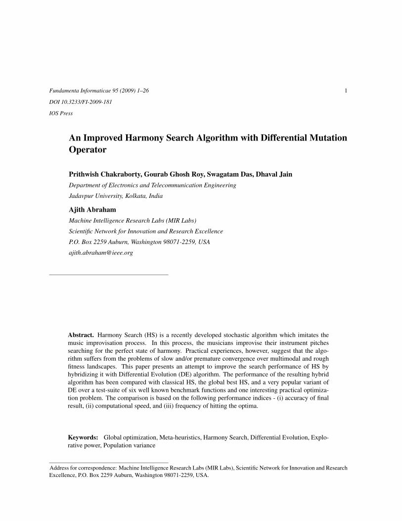
Most of the existing meta-heuristic algorithms imitate natural, scientific phenomena, e.g. physical an-nealing of metal plates in simulated annealing, evolution in evolutionary algorithms and human memoryin tabu search. Following similar trend, a new meta-heuristic algorithm can be conceptualized from the
P. Chakraborty et al. / An Improved Harmony Search Algorithm with Differential Mutation Operator 3
Figure 1. Analogy between music improvisation and engineering optimization (figure adopted from [8])
music improvisation process where musicians improvise their instruments’ pitches searching for a per-fect state of harmony. Although the estimation of a harmony is aesthetic and subjective, on the otherhand, there are several theorists who have provided the standard of harmony estimation: Greek philoso-pher and mathematician Pythagoras (582 – 497BC) worked out the frequency ratios (or string lengthratios with equal tension) and found that they had a particular mathematical relationship, after research-ing what notes sounded pleasant together. The octave was found to be a 1:2 ratio and what we today calla fifth to be a 2:3 ratio; French composer Leonin (1135 – 1201) is the first known significant composerof polyphonic “organum” which involved a simple doubling of the chant at an interval of a fifth or fourthabove or below; and French composer Jean-Philippe Rameau (1683 – 1764) established the classicalharmony theories in the book “Treatise on Harmony”, which still form the basis of the modern study oftonal harmony [24].
In engineering optimization, the estimation of a solution is carried out by putting values of deci-sion variables to objective function or fitness function and evaluating the function value with respect toseveral aspects such as cost, efficiency, and/or error. Just like music improvisation seeks a best state(fantastic harmony) determined by an aesthetic standard, optimization process seeks a best state (globaloptimum) determined by objective function evaluation; the pitch of each musical instrument determinesthe aesthetic quality, just as the objective function value is determined by the set of values assigned toeach decision variable; aesthetic sound quality can be improved practice after practice, objective functionvalue can be improved iteration by iteration. The HS meta-heuristic algorithm was derived based on nat-ural musical performance processes that occur when a musician searches for a perfect state of harmony,such as during jazz improvisation.
The analogy between music improvisation and engineering optimization is illustrated in Figure 1.Each music player (saxophonist, double bassist, and guitarist) can correspond to each decision variable(x1, x2, x3) and the range of each music instrument (saxophone = {Do, Re, Mi}; double bass = {Mi, Fa,Sol}; and guitar = {Sol, La, Si}) corresponds to the range of each variable value (x1 = {100, 200, 300};x2 = {300, 400, 500}; and x3 = {500, 600, 700}). If the saxophonist toots the note Re, the doublebassist plucks Mi, and the guitarist plucks Si, their notes together make a new harmony (Re, Mi, Si). Ifthis new harmony is better than existing harmony, the new one is kept. Likewise, the new solution vector(200mm, 300mm, 700mm) is kept if it is better than existing harmony in terms of objective functionvalue. The harmony quality is improved by practice after practice.
Similarly in engineering optimization, each decision variable initially chooses any value within thepossible range, together making one solution vector. If all the values of decision variables make a goodsolution, that experience is stored in each variable’s memory and the possibility to make a good solution
4 P. Chakraborty et al. / An Improved Harmony Search Algorithm with Differential Mutation Operator
is also increased next time. When a musician improvises one pitch, he (or she) has to follow any one ofthree rules:
1. playing any one pitch from his (or her) memory,
2. playing an adjacent pitch of one pitch from his (or her) memory, and
3. playing totally random pitch from the possible range of pitches.
Similarly, when each decision variable chooses one value in the HS algorithm, it follows any one of threerules:
1. choosing any one value from the HS memory (defined as memory considerations),
2. choosing an adjacent value of one value from the HS memory (defined as pitch adjustments) and
3. choosing totally random value from the possible range of values (defined as randomization).
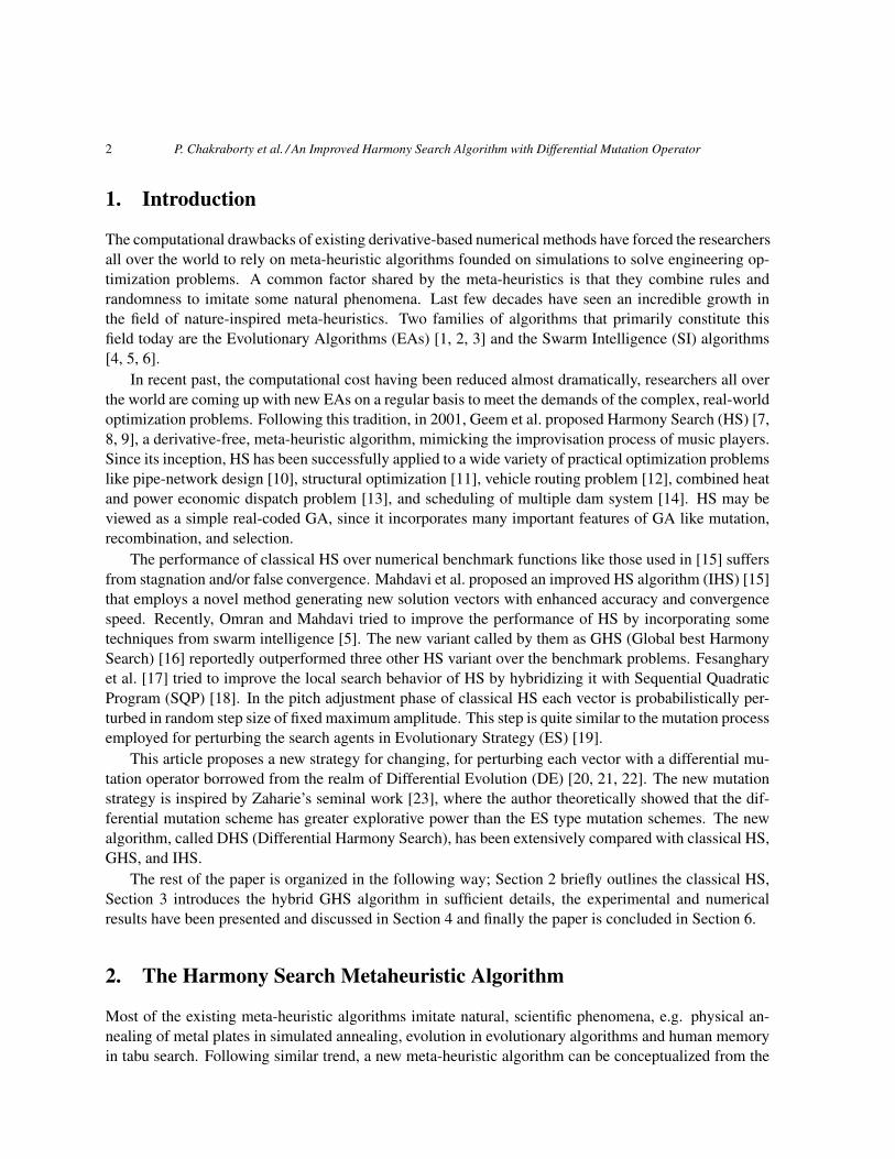
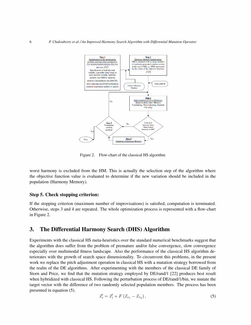
According to the above concept, the HS meta-heuristic algorithm consists of the following five steps[7, 8]:
Step 1 : Initialization of the optimization problem and algorithm parameters.
Step 2 : Harmony memory initialization.
Step 3 : New Harmony improvisation.
Step 4 : Harmony memory update.
Step 5 : Repetition of Steps 3 and 4 until the termination criterion is satisfied.
Note that in what follows we shall denote vectors in bold.
Step 1. Initialization of the optimization problem and algorithm parameters:
In the first step, the optimization problem is specified as follows:
Minimize (or Maximize) f(~x) (1)
subjected to xi ∈ Xi, i = 1, 2, . . . , N .Where f(·)is a scalar objective function to be optimized; ~x is a solution vector composed of decision
variables xi; Xi is the set of possible range of values for each decision variable xi (continuous decisionvariable), that is Lxi ≤ Xi ≤ Uxi, where Lxi and Uxi are the lower and upper bounds for each decisionvariable respectively, and N is the number of decision variables. In addition, the control parametersof HS are also specified in this step. These parameters are the Harmony Memory Size (HMS) i.e. thenumber of solution vectors (population members) in the harmony memory (in each generation); HarmonyMemory Considering Rate (HMCR); Pitch Adjusting Rate (PAR ); and the Number of Improvisations(NI) or stopping criterion.

P. Chakraborty et al. / An Improved Harmony Search Algorithm with Differential Mutation Operator 5
Step 2. Harmony memory initialization:
In the 2nd step each component of each vector in the parental population (Harmony Memory), which isof size HMS, is initialized with a uniformly distributed random number between the upper and lowerbounds [Lxi, Uxi], where 1 ≤ i ≤ N . This is done for the i-th component of the j-th solution vectorusing the following equation:
xji = Lxi + rand(0, 1) · (Uxi − Lxi) (2)
where j = 1, 2, 3, . . . ,HMS and rand(0, 1) is a uniformly distributed random number between 0 and1 and it is instantiated a new for each component of each vector.
Step 3. New Harmony improvisation:
In this step, a new harmony vector ~x′ = (x′1, x′2, x′3, x′4, . . . , x
′N ) is generated based on three rules:
(1) memory consideration, (2) pitch adjustment, and (3) random selection. Generating a new harmonyis called ‘improvisation’. In the memory consideration, the value of the first decision variable x′1 forthe new vector is chosen from any of the values already existing in the current HM i.e. from theset{x1
1, . . . , xHMS1 }, with a probabilityHMCR. Values of the other decision variables x′2, x
′3, x′4, . . . , x
′N
are also chosen in the same manner. The HMCR, which varies between 0 and 1, is the rate of choos-ing one value from the previous values stored in the HM , while (1 −HMCR)is the rate of randomlyselecting a fresh value from the possible range of values.
x′i ←
{xi ∈ {x1
i , x2i , x
3i , . . . , x
HMSi } with probability HMCR
xi ∈ Xi with probability (1−HMCR).(3)
For example, an HMCR = 0.80 indicates that the HS algorithm will choose the decision variablevalue from historically stored values in theHM with an 80% probability or from the entire possible rangewith a 20% probability. Every component obtained by the memory consideration is further examined todetermine whether it should be pitch-adjusted. This operation uses the parameter PAR (which is therate of pitch adjustment) as follows:
Pitch Adjusting Decision for
x′i =
{x′i ± rand(0, 1) · bw with probability PAR,x′i with probability (1− PAR),
(4)
where bw is an arbitrary distance bandwidth (a scalar number) and rand() is a uniformly distributedrandom number between 0 and 1. Evidently step 3 is responsible for generating new potential variationin the algorithm and is comparable to mutation in standard EAs. Thus either the decision variable isperturbed with a random number between 0 and bw or otherwise it is left unaltered with a probabilityPAR or else it is left unchanged with probability (1− PAR).
Step 4. Harmony memory update:
If the new harmony vector ~x′ = (x′1, x′2, x′3, x′4, . . . , x
′N ) is better than the worst harmony in the HM,
judged in terms of the objective function value, the new harmony is included in the HM and the existing
6 P. Chakraborty et al. / An Improved Harmony Search Algorithm with Differential Mutation Operator
Figure 2. Flow-chart of the classical HS algorithm
worst harmony is excluded from the HM. This is actually the selection step of the algorithm wherethe objective function value is evaluated to determine if the new variation should be included in thepopulation (Harmony Memory).
Step 5. Check stopping criterion:
If the stopping criterion (maximum number of improvisations) is satisfied, computation is terminated.Otherwise, steps 3 and 4 are repeated. The whole optimization process is represented with a flow-chartin Figure 2.
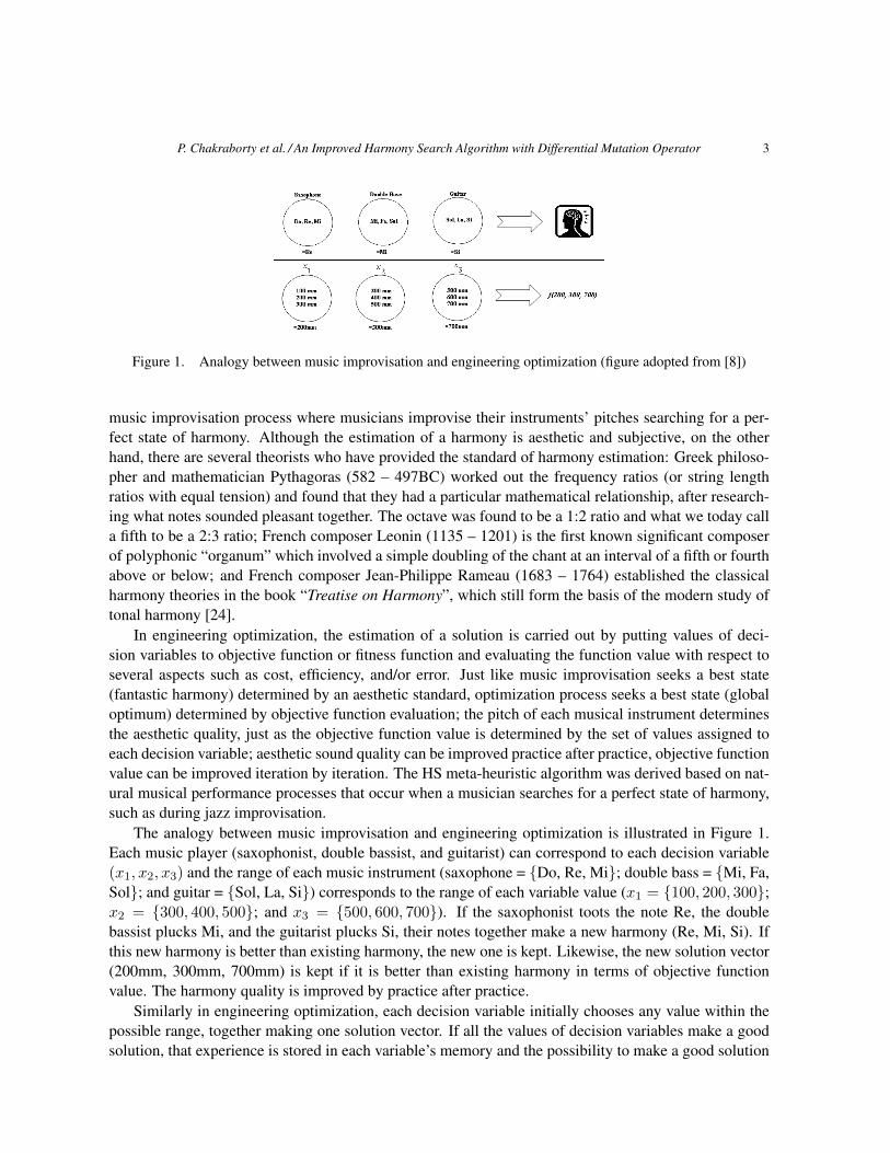
3. The Differential Harmony Search (DHS) Algorithm
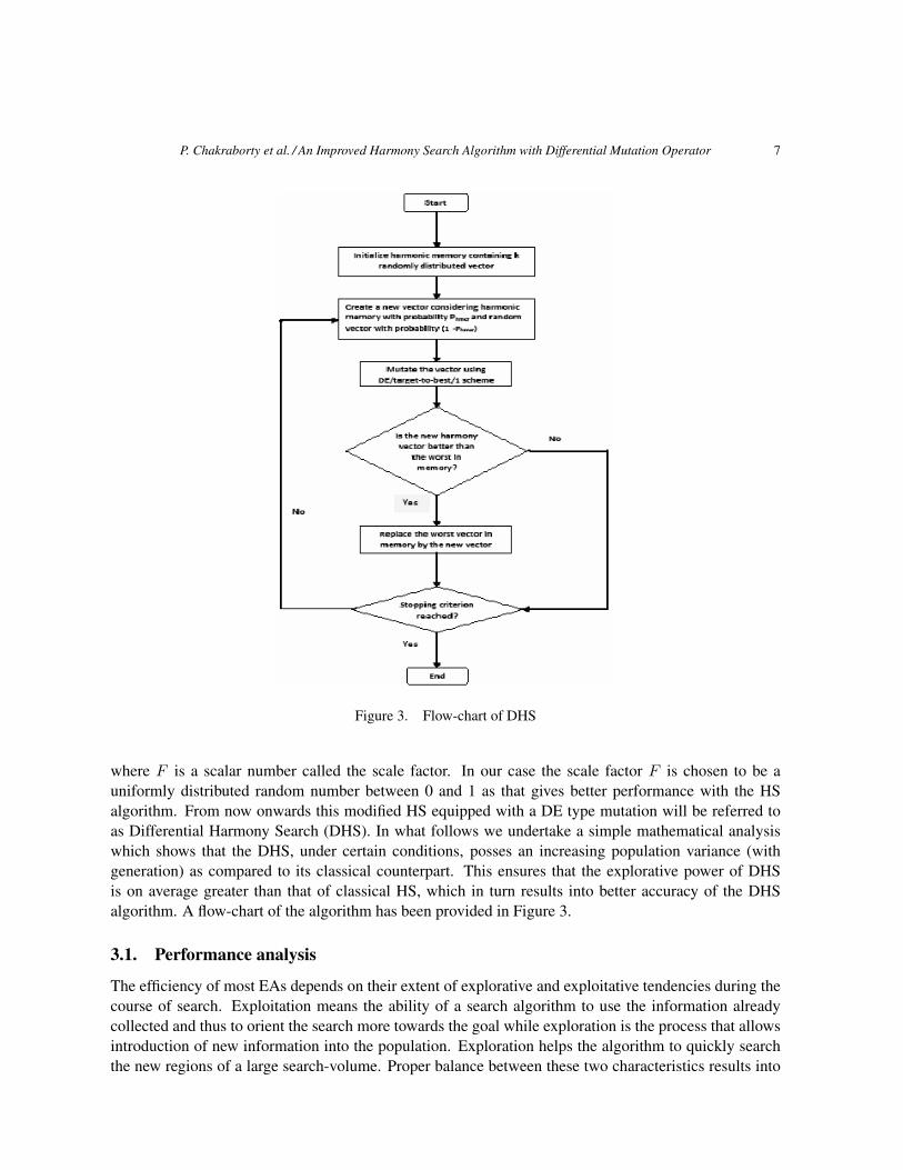
Experiments with the classical HS meta-heuristics over the standard numerical benchmarks suggest thatthe algorithm does suffer from the problem of premature and/or false convergence, slow convergenceespecially over multimodal fitness landscape. Also the performance of the classical HS algorithm de-teriorates with the growth of search space dimensionality. To circumvent this problems, in the presentwork we replace the pitch adjustment operation in classical HS with a mutation strategy borrowed fromthe realm of the DE algorithms. After experimenting with the members of the classical DE family ofStorn and Price, we find that the mutation strategy employed by DE/rand/1 [22] produces best resultwhen hybridized with classical HS. Following the perturbation process of DE/rand/1/bin, we mutate thetarget vector with the difference of two randomly selected population members. The process has beenpresented in equation (5).
~x′i = ~x′i + F (~xr1 − ~xr2) , (5)
P. Chakraborty et al. / An Improved Harmony Search Algorithm with Differential Mutation Operator 7
Figure 3. Flow-chart of DHS
where F is a scalar number called the scale factor. In our case the scale factor F is chosen to be auniformly distributed random number between 0 and 1 as that gives better performance with the HSalgorithm. From now onwards this modified HS equipped with a DE type mutation will be referred toas Differential Harmony Search (DHS). In what follows we undertake a simple mathematical analysiswhich shows that the DHS, under certain conditions, posses an increasing population variance (withgeneration) as compared to its classical counterpart. This ensures that the explorative power of DHSis on average greater than that of classical HS, which in turn results into better accuracy of the DHSalgorithm. A flow-chart of the algorithm has been provided in Figure 3.
3.1. Performance analysis
The efficiency of most EAs depends on their extent of explorative and exploitative tendencies during thecourse of search. Exploitation means the ability of a search algorithm to use the information alreadycollected and thus to orient the search more towards the goal while exploration is the process that allowsintroduction of new information into the population. Exploration helps the algorithm to quickly searchthe new regions of a large search-volume. Proper balance between these two characteristics results into
8 P. Chakraborty et al. / An Improved Harmony Search Algorithm with Differential Mutation Operator
enhanced performance [25]. Generally EAs explore the search space by the (genetic) search operators,while exploitation is done via selection that promotes better individuals to the next generation.
Expected value of population variance form one generation to another generation is a good estimateof the explorative power of a stochastic search algorithm. In this paper we analyze the evolution of thepopulation-variance of HS and its influence on the explorative power of the algorithm. We first find ananalytical expression for the population-variance of DHS and then compare it with the expected popu-lation variance of classical HS to show that the formal algorithm possesses greater explorative power.Since in HS type algorithms, each dimension is perturbed independently, without the loss of generality,we carry forward our analysis for single-dimensional population members.
In DHS the perturbations are made independently for each component. As such, without loss ofgenerality, we may conduct the analysis on one-dimensional elements. Let us consider a population ofscalars x = {x1, x2, . . . , xm} with elements x1 ∈ R. The variance of this population is given by:
V ar(x) =1m
m∑i=1
(xi − x)2 = x2 − x2 (6)
where, x is population mean and x2 is quadratic population mean.If the elements of the population are affected by some random elements, V ar(x) will be a random
variable and E[V ar(x)] will be the measure of the explorative power. Variance of DHS is calculatedbelow with the following assumptions.
Theorem 3.1. Let x = {x1, x2, . . . , xm} be the current population, y be an intermediate vector obtainedafter random selection and harmony memory consideration and z the vector obtained after pitch adjustingy. Let w = {w1, w2, . . . , wm} be the final population after selection. If
PHMCR = Harmonic Memory Consideration Probability
and, we consider the allowable range for the new values of x is {xmin, xmax} where xmax = a, xmax =−a and the required random numbers are continuously uniformly distributed between 0 and 1, then
E[V (w)] =23V (x) +
a2
3
(m− 1m
)(1− PHMCR)+
+x2
m
(PHMCR +
m− 1m
)− x2PHMCR
m2{PHMCR + 2(m− 1)}
Proof:Here x = {x1, x2, . . . , xm} is the current population. So the population mean x is given by
x =1m
m∑i=1
xi (7)
And, quadratic population mean x2 as
x2 =1m
m∑i=1
x2i (8)
P. Chakraborty et al. / An Improved Harmony Search Algorithm with Differential Mutation Operator 9
y is an intermediate vector obtained after random selection and harmony memory consideration. It isobtained as:
y =
{xl with probability PHMCR
xr with probability (1− PHMCR),(9)
where l and k are two elements of {1, 2, . . . ,m} and xr is a new random number in the allowable range{xmin, xmax} or {−a, a} and the index k is a random variable with values in {1, 2, . . . ,m}, with theprobability Pk = P (i = k) = 1
m .Therefore,
E(xl) =∑l
xlPl =1m
∑l
xl = x
E(x2l ) =
∑l
x2l Pl =
1m
∑l
x2l = x2
(10)
Similarly, those for xr may be given as in Eq. (11) with detailed proof being provided in Appendix B.
E(xr) = 0
E(x2r) =
a2
3
(11)
Using Eqs. (10) and (11), the following relations can be inferred
E(y) = E(xl)PHMCR + E(xr)(1− PHMCR) = PHMCRx (12)
E(y2) = E(x2l )PHMCR + E(x2
r)(1− PHMCR) = x2PHMCR +a2
3(1− PHMCR) (13)
Now z is the vector obtained after mutating y. This has the following structure:
z = y + F (xβ1 − xβ2),
where F is a uniformly distributed random number varying between 0 and 1. As such following Ap-pendix A, we can say that
F = E(F ) =12
F 2 = E(F 2) =13
(14)
Also, xβ1 and xβ2 are two randomly chosen members from x such that β1 6= β2.Thus following equations hold
E(xβ1) = E(xβ2) = x
E[x2β1
] = E[x2β2
] = x2
E[xβ1xβ2 ] =1
m(m− 1)
{(mx)2 −mx2
} (15)
10 P. Chakraborty et al. / An Improved Harmony Search Algorithm with Differential Mutation Operator
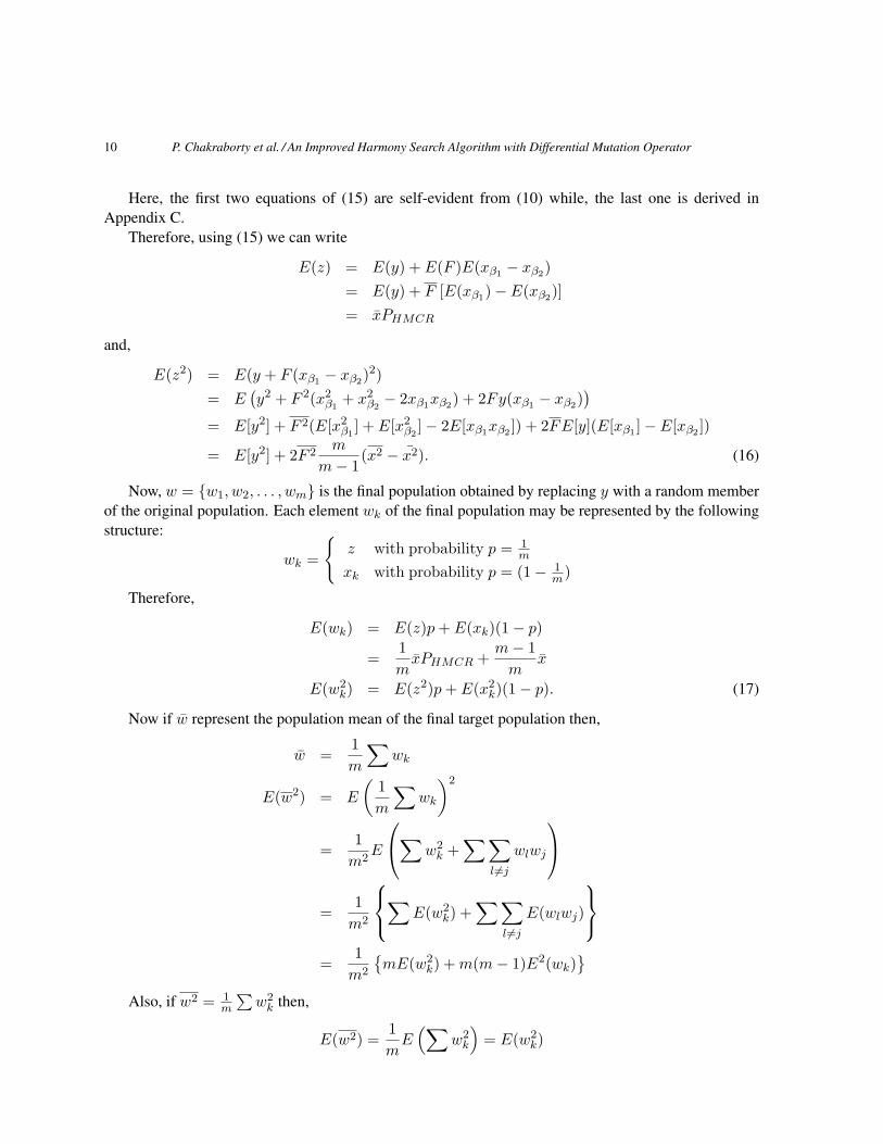
Here, the first two equations of (15) are self-evident from (10) while, the last one is derived inAppendix C.
Therefore, using (15) we can write
E(z) = E(y) + E(F )E(xβ1 − xβ2)= E(y) + F [E(xβ1)− E(xβ2)]= xPHMCR
and,
E(z2) = E(y + F (xβ1 − xβ2)2)= E
(y2 + F 2(x2
β1+ x2
β2− 2xβ1xβ2) + 2Fy(xβ1 − xβ2)
)= E[y2] + F 2(E[x2
β1] + E[x2
β2]− 2E[xβ1xβ2 ]) + 2FE[y](E[xβ1 ]− E[xβ2 ])
= E[y2] + 2F 2m
m− 1(x2 − x2). (16)
Now, w = {w1, w2, . . . , wm} is the final population obtained by replacing y with a random memberof the original population. Each element wk of the final population may be represented by the followingstructure:
wk =
{z with probability p = 1
m
xk with probability p = (1− 1m)
Therefore,
E(wk) = E(z)p+ E(xk)(1− p)
=1mxPHMCR +
m− 1m
x
E(w2k) = E(z2)p+ E(x2
k)(1− p). (17)
Now if w represent the population mean of the final target population then,
w =1m
∑wk
E(w2) = E
(1m
∑wk
)2
=1m2
E
∑w2k +
∑∑l 6=j
wlwj
=
1m2
∑E(w2k) +
∑∑l 6=j
E(wlwj)
=
1m2
{mE(w2
k) +m(m− 1)E2(wk)}
Also, if w2 = 1m
∑w2k then,
E(w2) =1mE(∑
w2k
)= E(w2
k)
P. Chakraborty et al. / An Improved Harmony Search Algorithm with Differential Mutation Operator 11
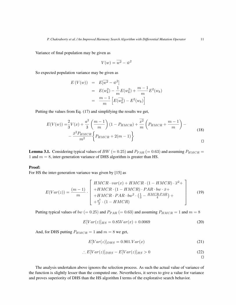
Variance of final population may be given as
V (w) = w2 − w2
So expected population variance may be given as
E (V (w)) = E[w2 − w2]
= E(w2k)−
1mE(w2
k) +m− 1m
E2(wk)
=m− 1m
[E(w2
k)− E2(wk)
]Putting the values from Eq. (17) and simplifying the results we get,
E(V (w)) =23V (x) +
a2
3
(m− 1m
)(1− PHMCR) +
x2
m
(PHMCR +
m− 1m
)−
− x2PHMCR
m2
{PHMCR + 2(m− 1)
} (18)
ut
Lemma 3.1. Considering typical values ofBW (= 0.25) and PPAR (= 0.63) and assuming PHMCR =1 and m = 8, inter-generation variance of DHS algorithm is greater than HS.
Proof:For HS the inter-generation variance was given by [15] as
E(V ar(z)) =(m− 1)m
·
HMCR · var(x) +HMCR · (1−HMCR) · x2++HMCR · (1−HMCR) · PAR · bw · x++HMCR · PAR · bw2 ·
(13 −
HMCR·PAR4
)+
+a2
3 · (1−HMCR)
(19)
Putting typical values of bw (= 0.25) and PPAR (= 0.63) and assuming PHMCR = 1 and m = 8
E[V ar(z)]HS = 0.85V ar(x) + 0.0069 (20)
And, for DHS putting PHMCR = 1 and m = 8 we get,
E[V ar(z)]DHS = 0.901.V ar(x) (21)
∴ E[V ar(z)]DHS − E[V ar(z)]HS > 0 (22)ut
The analysis undertaken above ignores the selection process. As such the actual value of variance ofthe function is slightly lesser than the computed one. Nevertheless, it serves to give a value for varianceand proves superiority of DHS than the HS algorithm I terms of the explorative search behavior.
12 P. Chakraborty et al. / An Improved Harmony Search Algorithm with Differential Mutation Operator
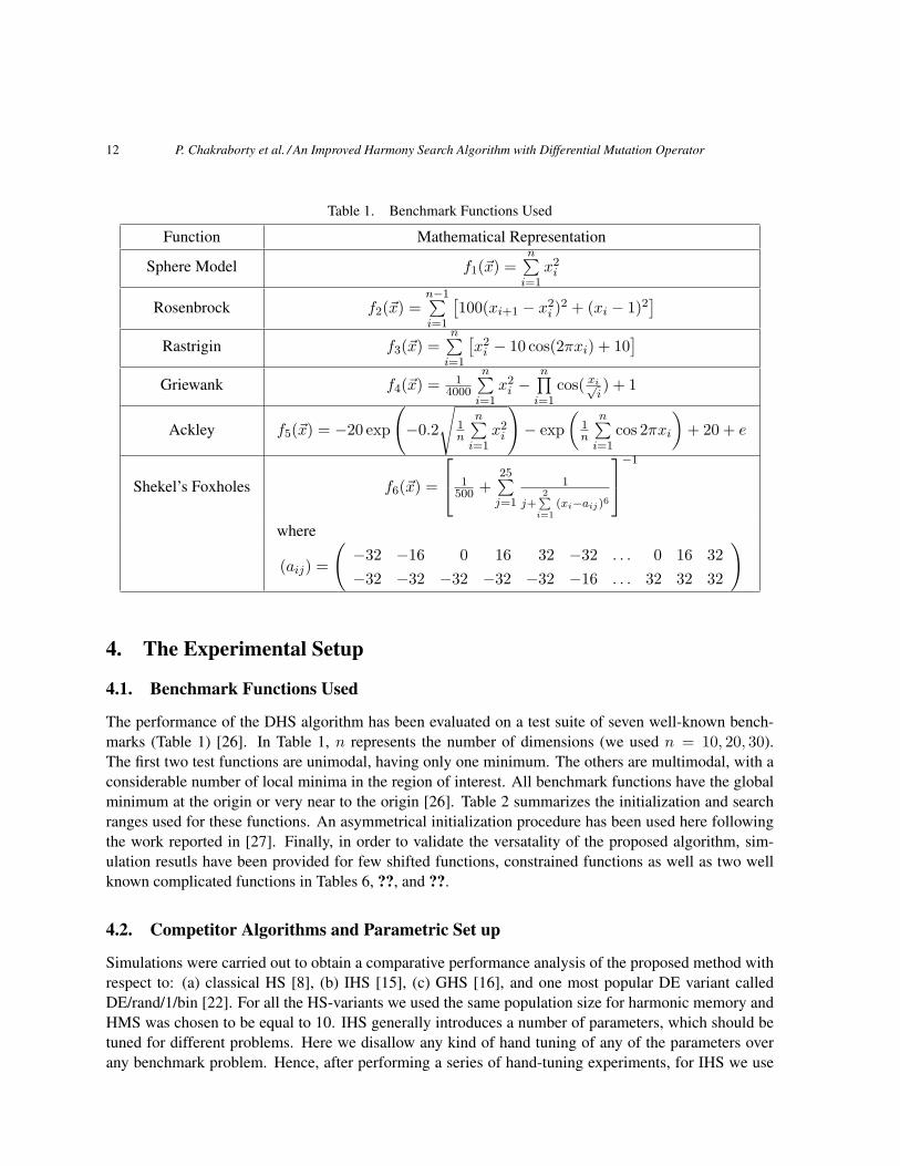
Table 1. Benchmark Functions Used
Function Mathematical Representation
Sphere Model f1(~x) =n∑i=1
x2i
Rosenbrock f2(~x) =n−1∑i=1
[100(xi+1 − x2
i )2 + (xi − 1)2
]Rastrigin f3(~x) =
n∑i=1
[x2i − 10 cos(2πxi) + 10
]Griewank f4(~x) = 1
4000
n∑i=1
x2i −
n∏i=1
cos( xi√i) + 1
Ackley f5(~x) = −20 exp
(−0.2
√1n
n∑i=1
x2i
)− exp
(1n
n∑i=1
cos 2πxi
)+ 20 + e
Shekel’s Foxholes f6(~x) =
1500 +
25∑j=1
1
j+2∑i=1
(xi−aij)6
−1
where
(aij) =
(−32 −16 0 16 32 −32 . . . 0 16 32−32 −32 −32 −32 −32 −16 . . . 32 32 32
)
4. The Experimental Setup
4.1. Benchmark Functions Used
The performance of the DHS algorithm has been evaluated on a test suite of seven well-known bench-marks (Table 1) [26]. In Table 1, n represents the number of dimensions (we used n = 10, 20, 30).The first two test functions are unimodal, having only one minimum. The others are multimodal, with aconsiderable number of local minima in the region of interest. All benchmark functions have the globalminimum at the origin or very near to the origin [26]. Table 2 summarizes the initialization and searchranges used for these functions. An asymmetrical initialization procedure has been used here followingthe work reported in [27]. Finally, in order to validate the versatality of the proposed algorithm, sim-ulation resutls have been provided for few shifted functions, constrained functions as well as two wellknown complicated functions in Tables 6, ??, and ??.
4.2. Competitor Algorithms and Parametric Set up
Simulations were carried out to obtain a comparative performance analysis of the proposed method withrespect to: (a) classical HS [8], (b) IHS [15], (c) GHS [16], and one most popular DE variant calledDE/rand/1/bin [22]. For all the HS-variants we used the same population size for harmonic memory andHMS was chosen to be equal to 10. IHS generally introduces a number of parameters, which should betuned for different problems. Here we disallow any kind of hand tuning of any of the parameters overany benchmark problem. Hence, after performing a series of hand-tuning experiments, for IHS we use
P. Chakraborty et al. / An Improved Harmony Search Algorithm with Differential Mutation Operator 13
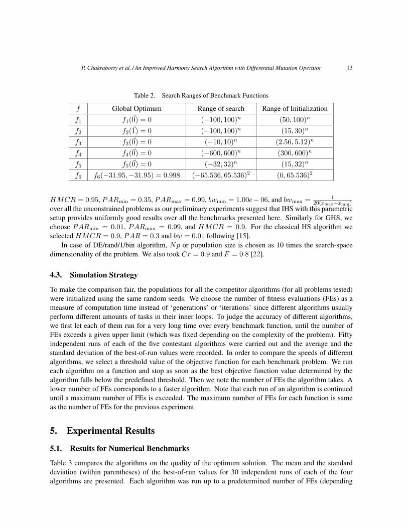
Table 2. Search Ranges of Benchmark Functions
f Global Optimum Range of search Range of Initialization
f1 f1(~0) = 0 (−100, 100)n (50, 100)n
f2 f2(~1) = 0 (−100, 100)n (15, 30)n
f3 f3(~0) = 0 (−10, 10)n (2.56, 5.12)n
f4 f4(~0) = 0 (−600, 600)n (300, 600)n
f5 f5(~0) = 0 (−32, 32)n (15, 32)n
f6 f6(−31.95,−31.95) = 0.998 (−65.536, 65.536)2 (0, 65.536)2
HMCR = 0.95, PARmin = 0.35, PARmax = 0.99, bwmin = 1.00e− 06, and bwmax = 120(xmax−xmin)
over all the unconstrained problems as our preliminary experiments suggest that IHS with this parametricsetup provides uniformly good results over all the benchmarks presented here. Similarly for GHS, wechoose PARmin = 0.01, PARmax = 0.99, and HMCR = 0.9. For the classical HS algorithm weselected HMCR = 0.9, PAR = 0.3 and bw = 0.01 following [15].
In case of DE/rand/1/bin algorithm, Np or population size is chosen as 10 times the search-spacedimensionality of the problem. We also took Cr = 0.9 and F = 0.8 [22].
4.3. Simulation Strategy
To make the comparison fair, the populations for all the competitor algorithms (for all problems tested)were initialized using the same random seeds. We choose the number of fitness evaluations (FEs) as ameasure of computation time instead of ‘generations’ or ‘iterations’ since different algorithms usuallyperform different amounts of tasks in their inner loops. To judge the accuracy of different algorithms,we first let each of them run for a very long time over every benchmark function, until the number ofFEs exceeds a given upper limit (which was fixed depending on the complexity of the problem). Fiftyindependent runs of each of the five contestant algorithms were carried out and the average and thestandard deviation of the best-of-run values were recorded. In order to compare the speeds of differentalgorithms, we select a threshold value of the objective function for each benchmark problem. We runeach algorithm on a function and stop as soon as the best objective function value determined by thealgorithm falls below the predefined threshold. Then we note the number of FEs the algorithm takes. Alower number of FEs corresponds to a faster algorithm. Note that each run of an algorithm is continueduntil a maximum number of FEs is exceeded. The maximum number of FEs for each function is sameas the number of FEs for the previous experiment.
5. Experimental Results
5.1. Results for Numerical Benchmarks
Table 3 compares the algorithms on the quality of the optimum solution. The mean and the standarddeviation (within parentheses) of the best-of-run values for 30 independent runs of each of the fouralgorithms are presented. Each algorithm was run up to a predetermined number of FEs (depending
14 P. Chakraborty et al. / An Improved Harmony Search Algorithm with Differential Mutation Operator
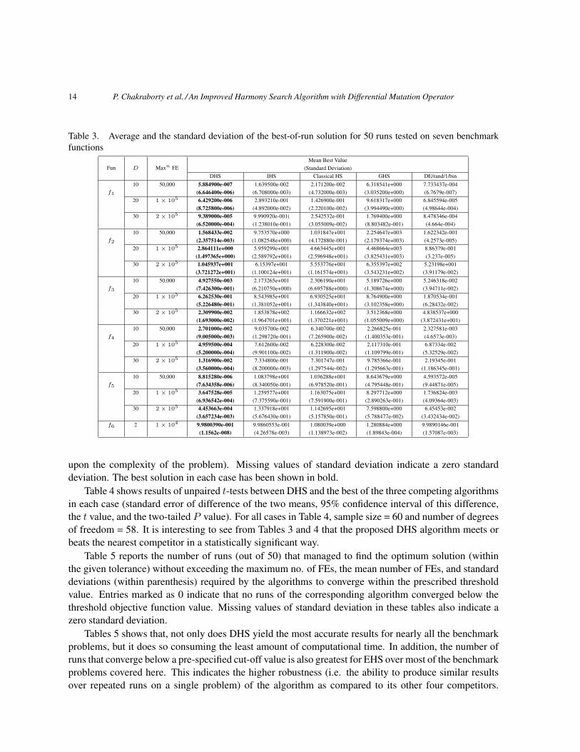
Table 3. Average and the standard deviation of the best-of-run solution for 50 runs tested on seven benchmarkfunctions
Fun D Maxn FEMean Best Value
(Standard Deviation)DHS IHS Classical HS GHS DE/rand/1/bin
f1
10 50,000 5.884900e-007 1.639500e-002 2.171200e-002 6.318541e+000 7.733437e-004(6.646400e-006) (6.708000e-003) (4.732000e-003) (3.035200e+000) (6.7679e-007)
20 1× 10⁵ 6.429200e-006 2.893210e-001 1.426900e-001 9.618317e+000 6.845594e-005(8.725800e-006) (4.892000e-002) (2.220100e-002) (3.994490e+000) (4.98644e-004)
30 2× 10⁵ 9.389000e-005 9.990920e-001( 2.542532e-001 1.769400e+000 8.478346e-004(6.520000e-004) (1.238010e-001) (3.055009e-002) (8.803482e-001) (4.664e-004)
f2
10 50,000 1.568433e-002 9.753570e+000 1.031847e+001 2.254647e+003 1.622342e-001(2.357514e-003) (1.082548e+000) (4.172880e-001) (2.179374e+003) (4.2573e-005)
20 1× 10⁵ 2.864111e+000 5.959299e+001 4.663445e+001 4.468664e+003 8.86379e-001(1.497365e+000) (2.589792e+001) (2.596948e+001) (3.825431e+003) (3.237e-005)
30 2× 10⁵ 1.045937e+001 6.15397e+001 5.553776e+001 6.355397e+002 5.23198e+001(3.721272e+001) (1.100124e+001) (1.161574e+001) (3.543231e+002) (3.91179e-002)
f3
10 50,000 4.927550e-003 2.173265e+001 2.306190e+001 5.189726e+000 5.246318e-002(7.426300e-001) (6.210750e+000) (6.695788e+000) (1.308674e+000) (3.94711e-002)
20 1× 10⁵ 6.262530e-001 8.543985e+001 6.930525e+001 8.764900e+000 1.870534e-001(5.226480e-001) (1.381052e+001) (1.343840e+001) (3.102358e+000) (6.28432e-002)
30 2× 10⁵ 2.309900e-002 1.853878e+002 1.166632e+002 3.512368e+000 4.838537e+000(1.693000e-002) (1.964701e+001) (1.370221e+001) (1.055009e+000) (3.872431e+001)
f4
10 50,000 2.701000e-002 9.035700e-002 6.340700e-002 2.266825e-001 2.327581e-003(9.005000e-003) (1.298720e-001) (7.265900e-002) (1.400353e-001) (4.6573e-003)
20 1× 10⁵ 4.959500e-004 7.612600e-002 6.228300e-002 2.117310e-001 6.87334e-002(5.200000e-004) (9.901100e-002) (1.311900e-002) (1.109799e-001) (5.32529e-002)
30 2× 10⁵ 1.316900e-002 7.334800e-001 7.301747e-001 9.785366e-001 2.19345e-001(3.560000e-004) (8.200000e-003) (1.297544e-002) (1.295663e-001) (1.186345e-001)
f5
10 50,000 8.815280e-006 1.083798e+001 1.036288e+001 8.643679e+000 4.593572e-005(7.634358e-006) (8.340050e-001) (6.978520e-001) (4.795448e-001) (9.44871e-005)
20 1× 10⁵ 3.647528e-005 1.259577e+001 1.163075e+001 8.297712e+000 1.736824e-003(6.936542e-004) (7.375590e-001) (7.591900e-001) (2.890263e-001) (4.09364e-003)
30 2× 10⁵ 4.453663e-004 1.337918e+001 1.142695e+001 7.598800e+000 6.45453e-002(3.657234e-003) (5.676430e-001) (5.157850e-001) (5.788477e-002) (3.432434e-002)
f6 2 1× 10⁴ 9.9800390e-001 9.9860553e-001 1.080039e+000 1.280884e+000 9.9890146e-001(1.1562e-008) (4.26578e-003) (1.138973e-002) (1.89843e-004) (1.57087e-003)
upon the complexity of the problem). Missing values of standard deviation indicate a zero standarddeviation. The best solution in each case has been shown in bold.
Table 4 shows results of unpaired t-tests between DHS and the best of the three competing algorithmsin each case (standard error of difference of the two means, 95% confidence interval of this difference,the t value, and the two-tailed P value). For all cases in Table 4, sample size = 60 and number of degreesof freedom = 58. It is interesting to see from Tables 3 and 4 that the proposed DHS algorithm meets orbeats the nearest competitor in a statistically significant way.
Table 5 reports the number of runs (out of 50) that managed to find the optimum solution (withinthe given tolerance) without exceeding the maximum no. of FEs, the mean number of FEs, and standarddeviations (within parenthesis) required by the algorithms to converge within the prescribed thresholdvalue. Entries marked as 0 indicate that no runs of the corresponding algorithm converged below thethreshold objective function value. Missing values of standard deviation in these tables also indicate azero standard deviation.
Tables 5 shows that, not only does DHS yield the most accurate results for nearly all the benchmarkproblems, but it does so consuming the least amount of computational time. In addition, the number ofruns that converge below a pre-specified cut-off value is also greatest for EHS over most of the benchmarkproblems covered here. This indicates the higher robustness (i.e. the ability to produce similar resultsover repeated runs on a single problem) of the algorithm as compared to its other four competitors.
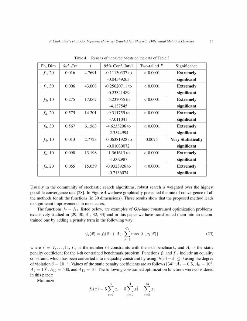
P. Chakraborty et al. / An Improved Harmony Search Algorithm with Differential Mutation Operator 15
Table 4. Results of unpaired t-tests on the data of Table 3
Fn, Dim Std. Err t 95% Conf. Intvl Two-tailed P Significance
f1, 20 0.016 4.7691 -0.11130337 to < 0.0001 Extremely-0.04549263 significant
f1, 30 0.006 43.008 -0.25620711 to < 0.0001 Extremely-0.23341489 significant
f3, 10 0.275 17.067 -5.237055 to < 0.0001 Extremely-4.137545 significant
f3, 20 0.575 14.201 -9.311759 to < 0.0001 Extremely-7.011041 significant
f3, 30 0.567 6.1563 -4.6233206 to < 0.0001 Extremely-2.3544994 significant
f4, 10 0.013 2.7723 -0.06381928 to 0.0075 Very Statistically-0.01030072 significant
f5, 10 0.090 13.198 -1.361613 to < 0.0001 Extremely-1.002987 significant
f4, 20 0.055 15.059 -0.9323926 to < 0.0001 Extremely-0.7136074 significant
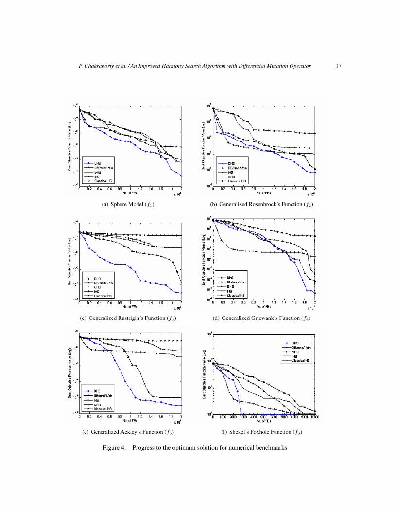
Usually in the community of stochastic search algorithms, robust search is weighted over the highestpossible convergence rate [28]. In Figure 4 we have graphically presented the rate of convergence of allthe methods for all the functions (in 30 dimensions). These results show that the proposed method leadsto significant improvements in most cases.
The functions f7 − f11, listed below, are examples of GA-hard constrained optimization problems,extensively studied in [29, 30, 31, 32, 33] and in this paper we have transformed them into an uncon-trained one by adding a penalty term in the following way:
ψi(~x) = fi(~x) +Ai ·Ci∑j=1
max {0, gj(~x)} (23)
where i = 7, . . . , 11, Ci is the number of constraints with the i-th benchnark, and Ai is the staticpenalty coefficient for the i-th contrained benchmark problem. Functions f8 and f11 include an equalityconstraint, which has been converted into inequality constraint by using |h(~x)− δ| ≤ 0 using the degreeof violation δ = 10−4. Values of the static penalty coefficients are as follows [34]: A7 = 0.5, A8 = 105,A9 = 104,A10 = 500, andA11 = 10. The following constrained optimization functions were consideredin this paper:
Minimize
f7(x) = 54∑i=1
xi − 54∑i=1
x2i −
13∑i=5
xi

16 P. Chakraborty et al. / An Improved Harmony Search Algorithm with Differential Mutation Operator
Table 5. Number of runs (out of 50) converging to the cut off fitness value for six benchmark functions
Fun D Maxn FENo. of runs converging to the cut off
DHS IHS Classical HS GHS DE/rand/1/bin
f1
10 1.00e-005 50,26253.20 50,32044.22 50,13423.68 42,41544.34 50,33932.64(445.34) (610.298) (341.827) (8532.261) (1450.492)
20 1.00e-005 31,68931.5 42,18298.21 44,7364.32 22,85367.86 34,46296.46(5712.65) (1340.34) (2235.83) (4540.12) (674.25)
30 1.00e-005 29,172228.72 45,84712.34 41,36523.46 16,74782.68 21,23876.62(6473.45) (8952.34) (7326.74) (6638.93) (7821.63)
f2
10 1.00e-003 24,454563.25 10,137628.60 0 11,167322.43 13,72874.34(7653.44) (10183.23) (0.4291) (67232.91)
20 1.00e-003 13,40943.68 0 1,48585 0 0(5831.84)
30 1.00e-003 8,83723.25 0 0 0 0
f3
10 1.00e-005 12,113817.52 0 0 0 0(12723.837) 0 0 0 0
20 1.00e-005 3,179834.33 0 0 0 0(21353.82)
30 1.00e-005 50,34983.68 32,39782.57 0 0 50,27474.24(4481.73) (7434.12) (5327.08)
f4
10 1.00e-005 50,83924.16 25,88731.04 0 0 50,73483.50(4028.47) (2139.57) (11142.76)
20 1.00e-005 43,129834.31 0 27,122833.73 0 0(10835.44) (9738.62)
30 1.00e-005 12,154982.76 0 19,167909.57 0 0(32432.87) (5672.89)
f5
10 1.00e-005 32,38769.46 21,37583.67 26,41029.75 0 0(3692.58) (7432.82) (3732.68)
20 1.00e-005 25,76093.80 17,75834.83 15,85734.46 0 0(4827.57) (6907.89) (5003.68)
30 1.00e-005 50,27243.44 32,29583.49 47,37263.92 7,48374.34 15,35563.46(447.03) (1241.57) (1832.45) (227.48) (1519.46)
P. Chakraborty et al. / An Improved Harmony Search Algorithm with Differential Mutation Operator 17
(a) Sphere Model (f1) (b) Generalized Rosenbrock’s Function (f2)
(c) Generalized Rastrigin’s Function (f3) (d) Generalized Griewank’s Function (f4)
(e) Generalized Ackley’s Function (f5) (f) Shekel’s Foxhole Function (f6)
Figure 4. Progress to the optimum solution for numerical benchmarks
18 P. Chakraborty et al. / An Improved Harmony Search Algorithm with Differential Mutation Operator
Subject to:
g1(x) = 2x1 + 2x2 + x10 + x11 − 10 ≤ 0g2(x) = 2x1 + 2x3 + x10 + x12 − 10 ≤ 0g3(x) = 2x2 + 2x3 + x11 + x12 − 10 ≤ 0g4(x) = −8x1 + x10 ≤ 0g5(x) = −8x2 + x11 ≤ 0g6(x) = −8x3 + x12 ≤ 0g7(x) = −2x4 − x5 + x10 ≤ 0g8(x) = −2x6 − x7 + x11 ≤ 0g9(x) = −2x8 − x9 + x12 ≤ 0
where the bounds are 0 ≤ xi ≤ 1 (i = 1, . . . , 9), 0 ≤ xi ≤ 100 (i = 10, 11, 12) and 0 ≤ x13 ≤1. The global optimum is at x∗ = (1, 1, 1, 1, 1, 1, 1, 1, 1, 3, 3, 3, 1) where f(x∗) = −15. Constraintsg1, g2, g3, g4, g5 and g6 are active.
Maximize
f8(x) =(√n)n n∏
i=1
xi
Subject to
h(x) =n∑i=1
x2i − 1 = 0,
where n = 10 and 0 ≤ xi ≤ 1, (i = 1, . . . , n). The global optimum is at
x∗ =1√n,
i = (1, . . . , n) where f(x∗) = 1Minimize
f9(x) = 5.3578547x22 + 0.8356891x1x5 + 37.293239x1 − 40792.141
Subject to:
g1(x) = 85.334407 + 0.0056858x2x5 + 0.0006262x1x4 − 0.0022053x3x5 − 92 ≤ 0g2(x) = −85.334407− 0.0056858x2x5 − 0.0006262x1x4 + 0.0022053x3x5 ≤ 0g3(x) = 80.51249 + 0.0071317x2x5 + 0.0029955x1x2 + 0.0021813x2
3 − 110 ≤ 0g4(x) = −80.51249− 0.0071317x2x5 − 0.0029955x1x2 − 0.0021813x2
3 + 90 ≤ 0g5(x) = 9.300961 + 0.0047026x3x5 + 0.0012547x1x3 + 0.0010985x3x4 − 25 ≤ 0g6(x) = −9.300961− 0.0047026x3x5 − 0.0012547x1x3 − 0.0010985x3x4 + 20 ≤ 0
where the bounds are 78 ≤ x1 ≤ 102, 33 ≤ x2 ≤ 45 and 27 ≤ xi ≤ 45, (i = 3, 4, 5). The globaloptimum is at x∗ = (78, 33, 29.995256025682, 45, 36.775812905788) where f(x∗) = −30665.539.Constraints g1 and g6 are active.
P. Chakraborty et al. / An Improved Harmony Search Algorithm with Differential Mutation Operator 19
Minimize
f10(x) = (x1 − 10)2 + 5(x2 − 12)2 + x43 + 3(x4 − 11)2 + 10x6
5 + 7x26 + x4
7 − 4x6x7 − 10x6 − 8x7
Subject to:g1(x) = −127 + 2x2
1 + 3x42 + x3 + 4x2
4 + 5x5 ≤ 0g2(x) = −282 + 7x1 + 3x2 + 10x2
3 + x4 − x5 ≤ 0g3(x) = −196 + 23x1 + x2
2 + 6x26 − 8x7 ≤ 0
g4(x) = 4x21 + x2
2 − 3x1x2 + 2x23 + 5x6 − 11x7 ≤ 0
where −10 ≤ xi ≤ 10, (i = 1, . . . , 7).The global optimum is at
x∗ = (2.330499, 1.951372,−0.4775414, 4.365726,−0.6244870, 1.038131, 1.594227)
where f(x∗) = 680.6300573. Constraints g1 and g4 are active.Minimize
f(x) = x21 + (x2 − 1)2
Subject to:h(x) = x2 − x2
1 = 0
where −1 ≤ x1 ≤ 1 and −1 ≤ x2 ≤ 1. The global optimum is at x∗ = (± 1√2, 1
2), where f(x∗) = 0.75.Besides comparing DHS with the two state-of-the-art HS variants we also take into account here
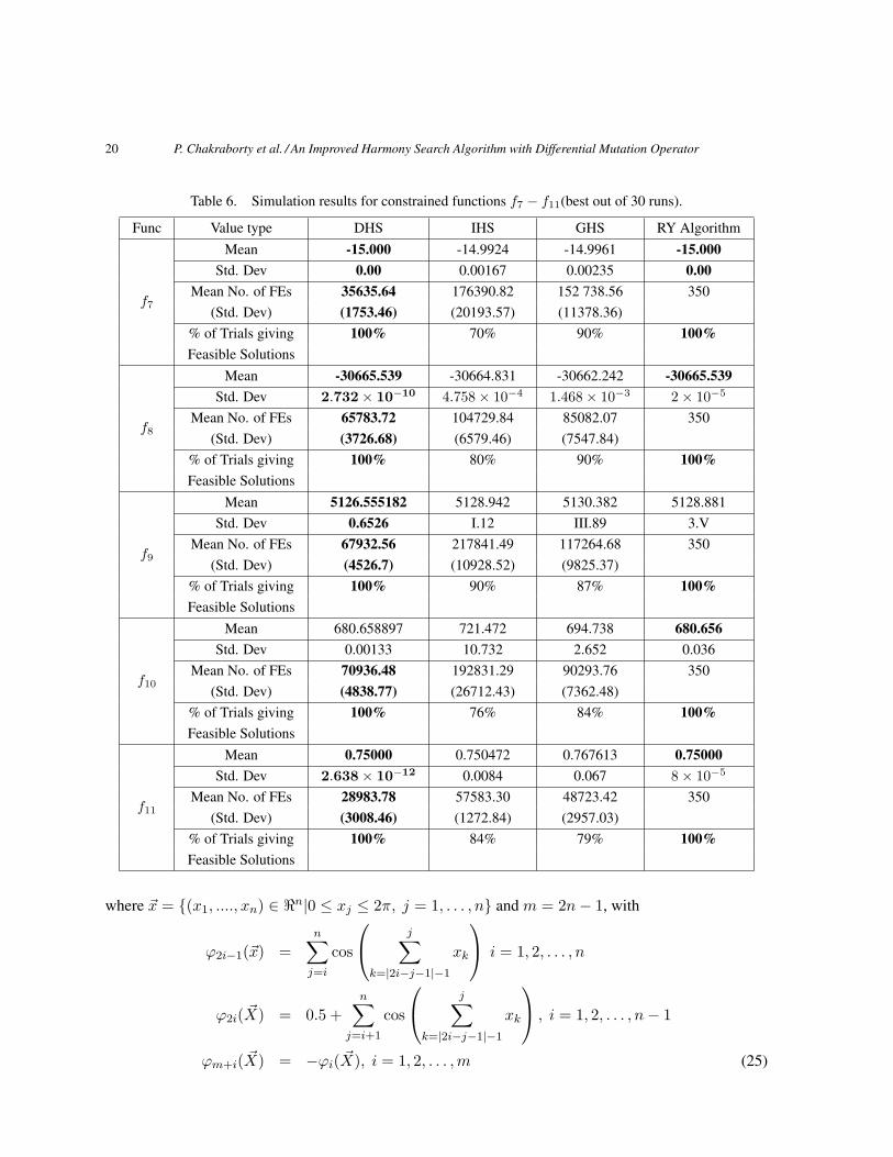
another evolutionary algorithm – RY [29] that is especially devised for optimizing constrained objectivefunctions. Numerical results for RY have been taken from [29]. Since the authors in [29] used a ter-mination criterion of 1750 generations (corresponding to 350 000 FEs) for the RY algorithm over thefive benchmarks we test here, in order to make the comparison fair, we compare both the qualities oftheir final solutions and the computational cost at the same. Accordingly, the termination criterion ofthe three HS variants is that the quality of the best solution cannot further be improved in the successive50 generations for each function. We reported the results for 30 independent runs of DHS, GHS, andIHS with different random seeds in table 6. In each run the three HS variants start from the same initialpopulation. The results for the RY algorithm are also for 30 independent trials for each function.
Table 6 indicates that DHS appears to be computationally more efficient than the two contestant HS-variants as well as the RY algorithm at least over the test-suite used here for constrained optimizationproblems.
5.2. Application to the Spread Spectrum Radar Poly-phase Code Design Problem
A famous problem of optimal design arises in the field of spread spectrum radar poly-phase codes [35].Such a problem is very well-suited for the application of global optimization algorithms like DE. Theproblem can be formally stated as:
Global min f(~x) = max{ϕ1(~x), . . . , ϕ2m(~x)}, (24)
20 P. Chakraborty et al. / An Improved Harmony Search Algorithm with Differential Mutation Operator
Table 6. Simulation results for constrained functions f7 − f11(best out of 30 runs).
Func Value type DHS IHS GHS RY Algorithm
f7
Mean -15.000 -14.9924 -14.9961 -15.000Std. Dev 0.00 0.00167 0.00235 0.00
Mean No. of FEs 35635.64 176390.82 152 738.56 350(Std. Dev) (1753.46) (20193.57) (11378.36)
% of Trials giving 100% 70% 90% 100%Feasible Solutions
f8
Mean -30665.539 -30664.831 -30662.242 -30665.539Std. Dev 2.732× 10⁻¹⁰ 4.758× 10⁻⁴ 1.468× 10⁻³ 2× 10⁻⁵
Mean No. of FEs 65783.72 104729.84 85082.07 350(Std. Dev) (3726.68) (6579.46) (7547.84)
% of Trials giving 100% 80% 90% 100%Feasible Solutions
f9
Mean 5126.555182 5128.942 5130.382 5128.881Std. Dev 0.6526 I.12 III.89 3.V
Mean No. of FEs 67932.56 217841.49 117264.68 350(Std. Dev) (4526.7) (10928.52) (9825.37)
% of Trials giving 100% 90% 87% 100%Feasible Solutions
f10
Mean 680.658897 721.472 694.738 680.656Std. Dev 0.00133 10.732 2.652 0.036
Mean No. of FEs 70936.48 192831.29 90293.76 350(Std. Dev) (4838.77) (26712.43) (7362.48)
% of Trials giving 100% 76% 84% 100%Feasible Solutions
f11
Mean 0.75000 0.750472 0.767613 0.75000Std. Dev 2.638× 10⁻¹² 0.0084 0.067 8× 10⁻⁵
Mean No. of FEs 28983.78 57583.30 48723.42 350(Std. Dev) (3008.46) (1272.84) (2957.03)
% of Trials giving 100% 84% 79% 100%Feasible Solutions
where ~x = {(x1, ...., xn) ∈ <n|0 ≤ xj ≤ 2π, j = 1, . . . , n} and m = 2n− 1, with
ϕ2i−1(~x) =n∑j=i
cos
j∑k=|2i−j−1|−1
xk
i = 1, 2, . . . , n
ϕ2i( ~X) = 0.5 +n∑
j=i+1
cos
j∑k=|2i−j−1|−1
xk
, i = 1, 2, . . . , n− 1
ϕm+i( ~X) = −ϕi( ~X), i = 1, 2, . . . ,m (25)

P. Chakraborty et al. / An Improved Harmony Search Algorithm with Differential Mutation Operator 21
Figure 5. f( ~X) of equation (22) for D = 2.
Table 7. Average and standard deviation (in parentheses) of the best-of-run solutions for 50 runs over the spreadspectrum radar poly-phase code design problem (number of dimensions n = 19 and n = 20). For all cases eachalgorithm was run up to 5× 10⁶ FEs.
N
Mean Best-of-run solution(standard deviation)
DE/rand/1/bin IHS HS GHS DHS Statistical Significance(by unpaired t-test)
19 7.4949e-01 7.5834e-01 7.5932e-01 7.6094e+01 7.4734e-01 Very(8.93e-03) (9.56e-04) (3.88e-05) (4.72e-03) (5.84e-04) Significant
20 8.5746e-01 8.3982e-01 8.3453e-01 8.4283e-01 8.0635e-01 Extremely(4.83e-03) (3.98e-03) (6.53e-04) (3.44e-02) (2.7343e-03) Significant
According to [35] the above problem has no polynomial time solution. The objective function forn = 2 is shown in Figure 5.
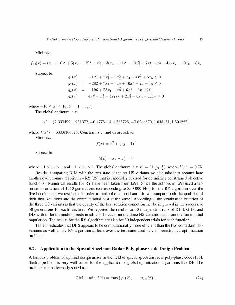
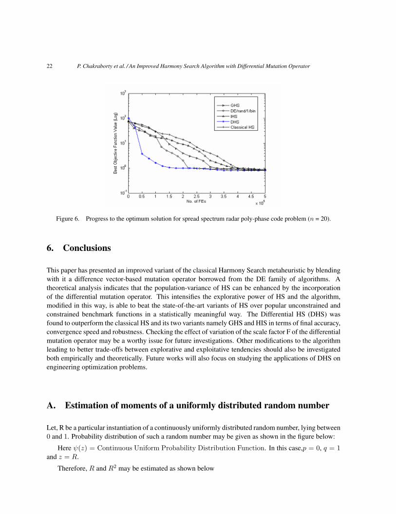
In Table 7, we show the mean and the standard deviation (within parentheses) of the best-of-runvalues for 30 independent runs of each of the six algorithms over the two most difficult instances ofthe radar poly-phase code design problem (for dimensions n = 19 and n = 20). Figure 6 graphicallypresents the rate of convergence of the contestant algorithms for the 20 - dimensional radar code designproblem.
Table 7 and Figure 6 clearly indicates that DHS can achieve more accurate and statistically betterresults as compared to all the contestants consuming less amount of computational time for this difficultreal life optimization problem.
22 P. Chakraborty et al. / An Improved Harmony Search Algorithm with Differential Mutation Operator
Figure 6. Progress to the optimum solution for spread spectrum radar poly-phase code problem (n = 20).
6. Conclusions
This paper has presented an improved variant of the classical Harmony Search metaheuristic by blendingwith it a difference vector-based mutation operator borrowed from the DE family of algorithms. Atheoretical analysis indicates that the population-variance of HS can be enhanced by the incorporationof the differential mutation operator. This intensifies the explorative power of HS and the algorithm,modified in this way, is able to beat the state-of-the-art variants of HS over popular unconstrained andconstrained benchmark functions in a statistically meaningful way. The Differential HS (DHS) wasfound to outperform the classical HS and its two variants namely GHS and HIS in terms of final accuracy,convergence speed and robustness. Checking the effect of variation of the scale factor F of the differentialmutation operator may be a worthy issue for future investigations. Other modifications to the algorithmleading to better trade-offs between explorative and exploitative tendencies should also be investigatedboth empirically and theoretically. Future works will also focus on studying the applications of DHS onengineering optimization problems.
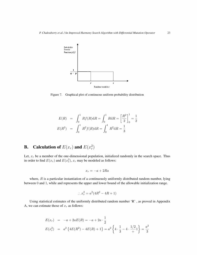
A. Estimation of moments of a uniformly distributed random number
Let, R be a particular instantiation of a continuously uniformly distributed random number, lying between0 and 1. Probability distribution of such a random number may be given as shown in the figure below:
Here ψ(z) = Continuous Uniform Probability Distribution Function. In this case,p = 0, q = 1and z = R.
Therefore, R and R2 may be estimated as shown below
P. Chakraborty et al. / An Improved Harmony Search Algorithm with Differential Mutation Operator 23
Figure 7. Graphical plot of continuous uniform probability distribution
E(R) =∫ 1
0Rf(R)dR =
∫ 1
0RdR =
[R2
2
]1
0
=12
E(R2) =∫ 1
0R2f(R)dR =
∫ 1
0R2dR =
13
B. Calculation of E(xr) and E(x2r)
Let, xr be a member of the one-dimensional population, initialized randomly in the search space. Thusin order to find E(xr) and E(x2
r), xr may be modeled as follows:
xr = −a+ 2Ra
where, R is a particular instantiation of a continuously uniformly distributed random number, lyingbetween 0 and 1, while and represents the upper and lower bound of the allowable initialization range.
∴ x2r = a2(4R2 − 4R+ 1)
Using statistical estimates of the uniformly distributed random number ‘R’ , as proved in AppendixA, we can estimate those of xr as follows:
E(xr) = −a+ 2aE(R) = −a+ 2a · 12
E(x2r) = a2
{4E(R2)− 4E(R) + 1
}= a2
{4 · 1
3− 4 · 1/2
+1}
=a2
3
24 P. Chakraborty et al. / An Improved Harmony Search Algorithm with Differential Mutation Operator
C. Calculation of E[xβ1xβ2
]
E[xβ1xβ2 ] =∑β1
β1 6=β2
∑β2
xβ1xβ2P (xβ1 , xβ2)
=1
m(m− 1)
∑β1
β1 6=β2
∑β2
xβ1xβ2
=1
m(m− 1)
{(∑xβ1
)2−∑
x2β1
}=
1m(m− 1)
{(mx)2 −mx2
}
References
[1] T. Back, D. Fogel, Z. Michalewicz, Handbook of Evolutionary Computation, Oxford Univ. Press, 1997.
[2] A.E. Eiben and J.E. Smith, Introduction to Evolutionary Computing, Springer, 2003.
[3] D. Ashlock, Evolutionary Computation for Modeling and Optimization, Springer, 2006.
[4] E. Bonabeau, M. Dorigo, and G. Theraulaz, Swarm Intelligence: From Natural to Artificial System, OxfordUniversity Press, New York, 1999.
[5] J. Kennedy, R. C. Eberhart, and Y. Shi, Swarm Intelligence, Morgan Kaufmann, San Francisco, CA, 2001.
[6] A. P. Engelbrecht, Fundamentals of Computational Swarm Intelligence, John Wiley & Sons, 2006.
[7] Z.W. Geem, J.H. Kim, and G.V. Loganathan, “A new heuristic optimization algorithm: harmony search”,Simulation 76(2), 60–68, 2001.
[8] K.S. Lee and Z.W. Geem, “A new meta-heuristic algorithm for continuous engineering optimization: har-mony search theory and practice”, Computer Methods in Applied Mechanics and Engineering, Eng, 194,3902–3933, 2004.
[9] Z. W. Geem (Ed.), Music-Inspired Harmony Search Algorithm: Theory and Applications, Studies in Compu-tational Intelligence, Springer, 2009.
[10] Z.W. Geem, J.H. Kim, and G.V. Loganathan, “Harmony search optimization: application to pipe networkdesign”, Int. J. Model. Simul, 22,(2), 125–133, 2002.
[11] K. S. Lee and Z.W. Geem, “A new structural optimization method based on the harmony search algorithm”,Computers and Structures, 82, pp. 781–798, Elsevier, 2004.
[12] Z. W. Geem, K. S. Lee, and Y. Park, “Application of harmony search to vehicle routing”, American Journalof Applied Sciences, 2(12), 1552-1557, 2005.
[13] A. Vasebi, M. Fesanghary, and S. M. T. Bathaeea, “Combined heat and power economic dispatch by harmonysearch algorithm”, International Journal of Electrical Power and Energy Systems, Vol. 29, No. 10, 713-719,Elsevier, 2007.
[14] Z. W. Geem, “Optimal scheduling of multiple dam system using harmony search algorithm”, Lecture Notesin Computer Science, Vol. 4507, 316-323, Springer, 2007.
P. Chakraborty et al. / An Improved Harmony Search Algorithm with Differential Mutation Operator 25
[15] M. Mahdavi, M. Fesanghary, and E. Damangir, “An improved harmony search algorithm for solving opti-mization problems”, Applied Mathematics and Computation, Vol. 188, 1567–1579, Elsevier Science, 2007.
[16] M. G. H. Omran and M. Mahdavi, “Global-best harmony search”, Applied Mathematics and Computation,Vol.198, 643–656, Elsevier Science, 2008.
[17] M. Fesanghary, M. Mahdavi, M. Minary-Jolandan, Y. Alizadeh, “Hybridizing sequential quadratic program-ming with HS algorithm for engineering optimization”, Computer Methods in Applied Mechanics and Engi-neering, Volume 197, Issues 33- 40, 1, pp. 3080-3091, Elsevier, June 2008.
[18] P.T. Boggs and J.W. Tolle, “Sequential quadratic programming”, Acta Numerica, 4, 1–52, 1995.
[19] H.-G. Beyer and H.-P. Schwefel, “Evolution strategies: a comprehensive introduction”, Natural Computing,1(1):3-52, 2002.
[20] R. Storn and K. V. Price, “Differential evolution - A simple and efficient adaptive scheme for global op-timization over continuous spaces”, Technical Report TR-95-012, ICSI, http://http.icsi.berkeley.edu/~storn/litera.html, 1995.
[21] , “Differential Evolution – a simple and efficient heuristic for global optimization over continuous spaces”,Journal of Global Optimization, 11(4) 341–359, 1997.
[22] R. Storn, K. V. Price, and J. Lampinen,Differential Evolution - A Practical Approach to Global Optimization,Springer, Berlin, 2005.
[23] D. Zaharie, “Critical values for the control parameters of differential evolution algorithms”, in R. Matousek,P. Osmera (eds.), Proc. of Mendel 2002, 8-th International Conference on Soft Computing, Brno,CzechRepublic, June 2002, pp. 62-67.
[24] R. Parncutt, Harmony: A Psychoacoustical Approach, Springer Verlag, 1989.
[25] A.E. Eiben and C.A. Schippers, “On evolutionary exploration and exploitation”, Fundamenta Informaticae,35, 1-16, IOS Press, 1998.
[26] X. Yao, Y. Liu, and G. Lin, “Evolutionary programming made faster,” IEEE Transactions on EvolutionaryComputation, 3(2), 82-102, July 1999.
[27] P. J. Angeline, “Evolutionary optimization versus particle swarm optimization: Philosophy and the perfor-mance difference,” Lecture Notes in Computer Science (vol. 1447), Proc. of 7th International Conferenceon. Evolutionary Programming – Evolutionary Programming VII, pp. 84-89, 1998
[28] A. E. Eiben, R. Hinterding, and Z. Michalewicz, “Parameter control in evolutionary algorithms,” IEEE Trans-actions on Evolutionary Computation, vol.3, no. 2, pp. 124-141, 1999.
[29] T. P. Runarsson and X. Yao, “Stochastic ranking for constrained evolutionary optimization,” IEEE Transac-tions on Evolutionary Computation, vol. 4, no. 3, pp. 284–294, Sep. 2000.
[30] S. A. Kazarlis, S. E. Papadakis, J. B. Theochairs, and V. Petridis, “Microgenetic algorithms as generalizedhill-climbing operators for GA optimization,” IEEE Transactions on Evolutionary Computation, vol. 5, no.3, pp. 204–217, Jun. 2001.
[31] S. Koziel and Z. Michalewicz, “Evolutionary algorithms, homomorphous mappings, and constrained param-eter optimization,” IEEE Transactions on Evolutionary Computation, vol. 7, no. 1, pp. 19–44, 1999.
[32] Z. Michalewicz and G. Nazhiyath, “Genocop III: A co-evolutionary algorithm for numerical optimizationproblems with nonlinear constraints,” in Proceedings of the 2nd IEEE Conference on Evolutionary Compu-tation. Piscataway, NJ: IEEE Press, vol. 2, pp. 647–651, 1995.
26 P. Chakraborty et al. / An Improved Harmony Search Algorithm with Differential Mutation Operator
[33] Z. Michalewicz and M. Schoenauer, “Evolutionary algorithms for constrained parameter optimization prob-lems,” Evolutionary Computation, vol. 4, no. 1, pp. 1–32, 1996.
[34] L. Jiao, Y. Li, M. Gong, and X. Zhang, “Quantum-inspired immune clonal algorithm for global numericaloptimization”, IEEE Transactions on System, Man, and Cybernetics, Part B, Vol. 38, No.5, 1234-1253, 2008.
[35] N. Mladenovic, J. Petrovic, V. Kovacevic-Vujicic, and M. Cangalovic, “Solving spread-spectrum radarpolyphase code design problem by tabu search and variable neighborhood search,” European Journal ofOperational Research, 153, 389-399, 2003.