AN ILLUSTRATED COLLECTION OF

GROUNDWATER PROBLEMS

prepared by

Sunderrajan Krishnan

as part of

Groundwater Governance in Asia: Theory and Practice

Contents

1. Introduction2. Numerical problems

i) Water balanceii) Hydraulic Headiii) Darcy’s Law

iv) Heterogeneityv) Aquifer Interactionvi) Specific yield, recharge and dischargevii) Well drawdownsviii) Interpreting head data

3. Computer Exercises3.1 Homogenous medium with reclining water table3.2 Heterogenous medium with reclining water table3.3 Two dimensional flow with constant head boundary conditions

4. Solutions to Numerical problems5. Solutions to Computer Exercises

Solution to 3.1Solution to 3.2Solution to 3.3

6. References7. Instructions and links for Softwares

About the front page

Wells represent the interaction between aquifers and society. They are a reflection of geology,culture and local engineering. Here some collection of pictures taken from across South Asia areproduced. These pictures are from: Basaltic, Alluvial, Sandy, Crystalline and Hilly aquifers of Nepal, and from Gujarat, MadhyaPradesh, Uttar Pradesh and Coimbatore in India.

Nomenclature

H: Hydraulic headi: Hydraulic gradientK : Hydraulic ConductivityKeff: Effective Conductivity

v: Darcy velocity

: Velocity of groundwater flow

q: Porosity

SY: Specific Yield

S: Storage Coefficient

: Change in Storage

1. Introduction

The purpose of this collection is to guide a beginner to groundwater hydrology through the basicconcepts in this subject. The problems begin with fundamentals of the subject and finally someproblems which test the comprehensiveness of understanding are developed. Most problems areillustrated and a real-world situation is related with the problem. The collection is part numerical-based, part software based. Computer tools have the power ofvisualization and extrapolation beyond the current problem. The purpose of computer-based

exercises are therefore to go beyond the problem developed here and use them to gain furtherunderstanding of concepts. Most of the numerical problems have been adapted from exercises provided in textbooks. Thereferences to the original problems have been provided along with the text here. In this version,further questions are added to some problems along with graphics and in some cases with change innumerical quantities. Any deviation from the original purpose of these problems developed by theoriginal authors is sincerely apologized and comments would be welcome on that. Solutions are provided to all problems in this collection. The earnest student is requested to applyutmost effort before having a look at the solutions. After all, these problems have a self-learningpurpose and merely reading the solutions will not serve the purpose of consolidating the theory. One should use this problem set in conjunction with a book on groundwater hydrology. Here wehave provided the basic formulae and concepts that are necessary to solve the problems here. Oneshould refer to textbooks to know more about the assumptions behind these formulae and situationsin which they can be used. Above all, one should treat a journey through these problems as a beginner’s training. For furtherexpansion into this fascinating subject, there is no replacement of a combination of field studies andrelating them to the theory. In that context, a knowledge of the numerical aspect of this subject andapplication of theory will enhance understanding and deepen interest in groundwater studies.

2. Numerical problems

i) Water balance

The hydrologic cycle is a continuous movement of water through the earth system at various timeand space scales. Within this cycle, any smaller system such as a river basin, an aquifer or a plantcan be seen as a conduit for water flow and storage. Unless water is created within any of thecomponents of this system, the change in storage should be reflected by water flowing in and out.

Equation 1

i.e the difference between flow out and flow in is the change in storage . This sameconcept can be applied at any time or space scale to derive various types of water balance equations.One such example for groundwater is:

Equation 2

where the change in storage in an aquifer is given by inputs in terms of flow inwards, recharge

from precipitation , and from return flow and outputs in terms of flow outwards laterally andvertically, Pumping P and Evapotranspiration E. In every specific example, we come across special requirements for modifying the water balance andone needs to tailor to the case keeping in mind the basic concept of mass balance.

Problem 1 Yearly groundwater balance over an aquifer

(Domenico and Schwartz, 1990)

Availability of electricity and subsidy for irrigation wells and pumps led to a sudden rise in pumpingin Indian Punjab. A research institution took up the task of analyzing the situation for one aquifer inthis state and the first step was to compute the annual groundwater balance for the past few years.From their calculation using field data and secondary information, they came up with the followingtable:

Table 1: Groundwater Balance over an Aquifer

Time Year Recharge from

Direct

Precipitation m3

Net Recharge

from Stream

flow m3

Discharge by

Pumping m3

Discharge by natural

Evapotranspiration m3

Change in

Ground Water

Storage m3

1 3 ! 107 0 0 3 ! 107 ?

2 3 ! 107 6 ! 105 1 ! 107 3 ! 107 ?

3 3 ! 107 1 ! 106 3 ! 107 9 ! 106 ?

4 2.8 ! 107 2 ! 106 3.5 ! 107 5 ! 106 ?

5 2.5 ! 107 3 ! 106 3.5 ! 107 3 ! 106 ?

6 3.5 ! 107 4 ! 106 4 ! 107 1 ! 106 ?

7 3.5 ! 107 4 ! 106 4.2 ! 107 1 ! 106 ?

8 3.5 ! 107 4 ! 106 4 ! 107 1 ! 106 ?

a) Compute the changes in groundwater storage. Is the aquifer being “overexploited”? How wouldyou qualify this statement?b) How much proportion of natural recharge is available for natural ET? How is this proportionchanging over the years? Why?

c) If this aquifer stores 1 x 106 m3 of water for every meter of depth, compute the changes in waterlevels. What is the trend in water levels over the years?d) Towards the end of Year 8, approximately how much would pumping need to be limited to so thatthere is no further drop in water levels?

Problem 2 Daily Soil moisture balance for a single storm

(give source) Often, we need detailed monitoring of individual storms so that the excess soil moisture and rechargehappening from such storms can be estimated. In such a case, atleast daily monitoring is needed.Jaisalmer lies in the Thar desert region of India. The rainfall here is highly variable and recharge togroundwater is minimal. Much of water evaporates and low amount of excess soil moisture isavailable. Data from a single storm in western arid part of India, Jaisalmer, for September 1976 isshown in the table. The initial soil moisture is 100.1 mm.

Day Rainfall Soil Moisture Actual ET

Moisture

surplus

1 mm mm mm mm

2 0 100.1 4.3 0

3 45 ? 6 0

4 26 ? 6.4 4.4

5 19 ? 6.4 12.6

6 19 ? 6.4 12.6

7 26 ? 6.4 19.6

8 0 ? 6.4 0

a) Compute the final soil moisture after the storm. Use this soil moisture balance equation: Soil moiscurr = Soil moisprev + Rainfallcurr – ETprev – Moisture surplusprev

where curr and prev denote the current and previous day. Apply this equation for each daysuccessively to compute the final soil moisture.

b) What is the total soil moisturesurplus? If 20% of this soil moisturesurplus infiltrates as recharge to thegroundwater, what is the rainfall-infiltration factor for this storm as awhole?

Table 2: Daily soil Moisture during a single

storm

ii) Hydraulic Head

The total head of groundwater at a given location is the sum of elevation head, pressure head andvelocity head (generally considered negligible). The total head above a datum is give by:

Equation 3

The elevation head is measured from a fixed datum, such as mean sea-level. The pressure head

could arise from different means such as pressure of from ponding or column of water above. Hydraulic gradient is any given direction is the gradient of the hydraulic head. It is denoted as i.

Problem 3 Measuring elevation and pressure head

(Domenico and Schwartz, 1990) Deep investigations of a confined aquifer revealed that the structure of the aquifer is in the form of afolded bed. The weight of the overload material on this syncline is such that the overburden pressureof material is much higher at the lower parts than at the higher parts leading to higher pore pressureat the lower parts of the aquifer. This was suspected to lead to groundwater flow against thetopographic gradient. In order to test this, a set of piezometers were installed in the aquifer takingcare to see that all of them reach this same confined aquifer.

In the accompanying diagram assume a hydraulic gradient of 100 ft/mile, with the water levelat point A being at an elevation of 900 feet above sea level. Assume further that the water level in allthe piezometers is at the top of the piezometers. The piezometers are located 1 mile apart. Calculatethe following blanks:

]

A B C D

Depth of Piezo(ft) 600 575 150 25

Total head(ft) 900 ? ? ?

Pressure head (ft) ? ? ? ?

Elevation head (ft) ? ? ? ?

Table 3: Head at different locations

Figure 1: Elevation and Pressure heads at different piezometers

iii) Darcy’s Law

As observed in experiment by Darcy, the velocity v of bulk of water moving across a cross-sectionwith hydraulic conductivity K and gradient i is simply (Todd, 2003),

Equation 4

with the negative sign denoting that the direction of decreasing gradient i is the same as direction offlow. This basic Darcy’s law is the basis of almost all current understanding of groundwater flowsystems apart from rapid flow through fractures and interflow

The primary properties of porous formations useful for understanding groundwater are porosity and hydraulic conductivity K. Porosity is the proportion of pores present in a soil or rock formation.Hydraulic conductivity is a measure of how fast water can flow through these pores, a measure of theconnectedness of the pores. It has units of velocity. One interesting aspect of hydraulic conductivityis that at the same location, it can have different values depending upon the direction of flow. Forexample, it might be easier to flow horizontally rather than vertically in a certain layeredsedimentary formation. This property of directional variation is called Anisotropy The velocity v derived from Darcy’s law is known as the Darcy velocity. The velocity of

groundwater flow through the pores of the medium with effective porosity is given by,

Equation 5

Problem 4 Darcy’s experiment

(Karanth, 1987)

It was Darcy’s original experiment with sand within a tube that led to the formulation of the law thatstands under his name. Even today, this experiment remains a technique to measure hydraulicconductivity in the laboratory. An inclined cylinder of 20 cm dia. is filled with saturated sand, with k = 10 m/day, isprovided with two piezometers 50 cm apart. The opening of the two piezometers have elevationheads of 50 and 30 cm from a common datum and corresponding water levels in the piezometers are32 and 26 cm. Estimate the flow rate through the cylinder.

Figure 2: Darcy’s experimental setup

Problem 5 Velocity of Groundwater flow

(Karanth, 1987)

Darcy’s law provides us with a bulk velocity that can be used for computing discharge through aporous medium. However in actuality, water flows in a tortuous path through pores and velocityfluctuations are observed at different scales. For some cases, detailed velocity profiles might beneeded as for transport of solutes. The average of all these velocity fluctuations is the ‘velocity ofgroundwater flow’ through the pores of the medium.

Determine the velocity of ground water flow given that: Average K of aquifer 11.0 m/day Effective porosity 0.10 Piezometric contour value at up-gradient point 164 m Piezometric contour value at down-gradient point 152 m Average distance between contours 18 km

Figure 3: Flow between two head contour lines

Problem 6 Paleo Aquifers and aquifer interaction

(Raghunath, 2002) In some aquifers, the velocity of groundwater transmission is very slow and water that is rechargedseveral thousand years back is found. Also there is slow interactions between different aquifers. Theage of water in different aquifers can be used as an indicator of flow-time between the aquifers.

During hydrogeological investigation two potential aquifers 32 km apart, were located, onebeing 5,000 years and the other 25,000 years old. They were found to be connected by a waterbearing stratum of 30 m thickness running inclined at 20 m/km. From a few observation wells, thehydraulic gradient was found to be 0.2 m/km. Determine the transmissibility of the water bearingstratum.

Figure 4: Flow between aquifers

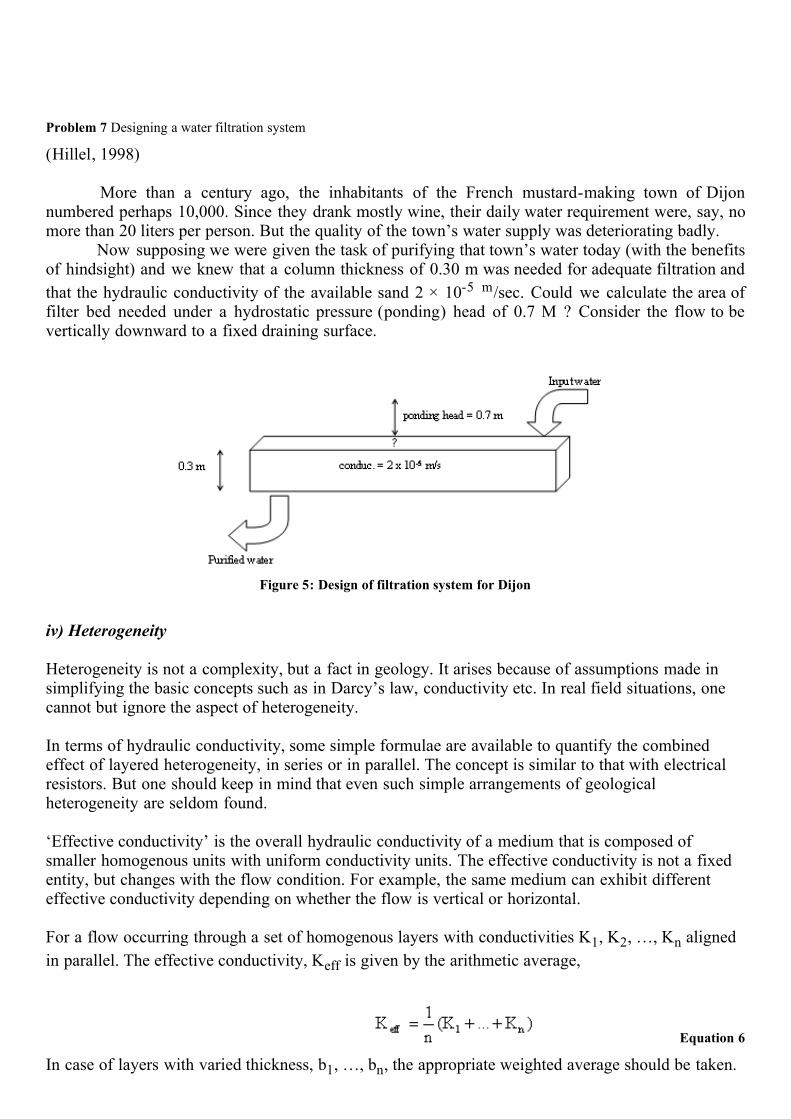
Problem 7 Designing a water filtration system

(Hillel, 1998) More than a century ago, the inhabitants of the French mustard-making town of Dijonnumbered perhaps 10,000. Since they drank mostly wine, their daily water requirement were, say, nomore than 20 liters per person. But the quality of the town’s water supply was deteriorating badly. Now supposing we were given the task of purifying that town’s water today (with the benefitsof hindsight) and we knew that a column thickness of 0.30 m was needed for adequate filtration and

that the hydraulic conductivity of the available sand 2 ! 10-5 m/sec. Could we calculate the area offilter bed needed under a hydrostatic pressure (ponding) head of 0.7 M ? Consider the flow to bevertically downward to a fixed draining surface.

Figure 5: Design of filtration system for Dijon

iv) Heterogeneity

Heterogeneity is not a complexity, but a fact in geology. It arises because of assumptions made insimplifying the basic concepts such as in Darcy’s law, conductivity etc. In real field situations, onecannot but ignore the aspect of heterogeneity. In terms of hydraulic conductivity, some simple formulae are available to quantify the combinedeffect of layered heterogeneity, in series or in parallel. The concept is similar to that with electricalresistors. But one should keep in mind that even such simple arrangements of geologicalheterogeneity are seldom found. ‘Effective conductivity’ is the overall hydraulic conductivity of a medium that is composed ofsmaller homogenous units with uniform conductivity units. The effective conductivity is not a fixedentity, but changes with the flow condition. For example, the same medium can exhibit differenteffective conductivity depending on whether the flow is vertical or horizontal. For a flow occurring through a set of homogenous layers with conductivities K1, K2, …, Kn aligned

in parallel. The effective conductivity, Keff is given by the arithmetic average,

Equation 6

In case of layers with varied thickness, b1, …, bn, the appropriate weighted average should be taken.

In case of layers with varied thickness, b1 bn, the appropriate weighted average should be taken.

For flow through layers in series, the effective conductivity Keff is given by the harmonic average,

Equation 7

A similar weighted average should be taken in case of layers with varied thicknesses. In general, forany flow condition, the effective conductivity lies between these two extremes of the arithmetic andharmonic averages.

Problem 8

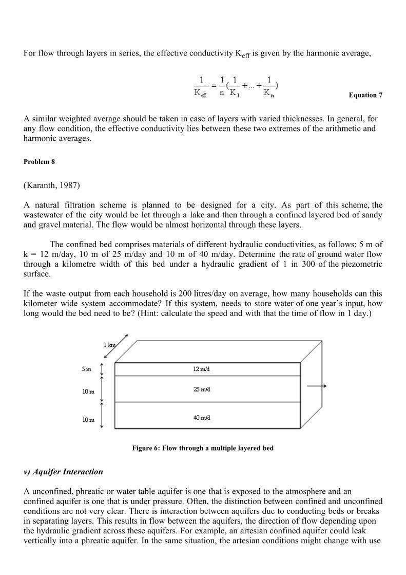
(Karanth, 1987) A natural filtration scheme is planned to be designed for a city. As part of this scheme, thewastewater of the city would be let through a lake and then through a confined layered bed of sandyand gravel material. The flow would be almost horizontal through these layers.

The confined bed comprises materials of different hydraulic conductivities, as follows: 5 m ofk = 12 m/day, 10 m of 25 m/day and 10 m of 40 m/day. Determine the rate of ground water flowthrough a kilometre width of this bed under a hydraulic gradient of 1 in 300 of the piezometricsurface. If the waste output from each household is 200 litres/day on average, how many households can thiskilometer wide system accommodate? If this system, needs to store water of one year’s input, howlong would the bed need to be? (Hint: calculate the speed and with that the time of flow in 1 day.)

Figure 6: Flow through a multiple layered bed

v) Aquifer Interaction

A unconfined, phreatic or water table aquifer is one that is exposed to the atmosphere and anconfined aquifer is one that is under pressure. Often, the distinction between confined and unconfinedconditions are not very clear. There is interaction between aquifers due to conducting beds or breaksin separating layers. This results in flow between the aquifers, the direction of flow depending uponthe hydraulic gradient across these aquifers. For example, an artesian confined aquifer could leakvertically into a phreatic aquifer. In the same situation, the artesian conditions might change with use

of the confined aquifer and there could be reversal of flow from the unconfined down into theconfined aquifer.

Problem 9 Leaky aquifer

(Karanth, 1987)

Often, we need to estimate the amount of vertical flow through aquifers separated by semi-permeablelayers. One way to do this is to have measurements of hydraulic head in the two aquifers. This ispossible if there are observation wells located nearby and tapping the two aquifers. This along withother information such as hydraulic conductivity of the aquifer material can give us an estimate ofthe flow due to interaction between the aquifers.

The Piezometric surface of a confined aquifer is 2 m below the water table in the unconfinedaquifer above. The two aquifers are separated by an aquitard of 3 m thickness. The water lies 15 mabove the top of the aquitard k of the aquitard is 0.08 m/day and that of the unconfined aquifer is 1.2m/day. Determine the recharge rate from the unconfined to the confined aquifer.

Figure 7: Leakage from unconfined into confined aquifer

Problem 10 Discharging aquifer

(Karanth, 1987) In case of confined aquifers under high pressure, there can be vertically upwards flow into theunconfined aquifer. Such direction of flow can also change seasonally with recharge/dischargeconditions.

In a ground water discharge area, a leaky artesian aquifer is overlain by a water table aquifer.Given that the piezometric head and the water table are, respectively, 20 and 12 m above the top ofthe artesian aquifer and the vertical hydraulic conductivity of the water table aquifer 1.2 m/day , findthe rate of leakage. Also, find the head in a piezometer with its bottom 3 m above the top of theaquifer

Figure 8: Discharging flow from artesian aquifer into unconfined aquifer

vi) Specific yield, recharge and discharge

Not all the water present in rocks however, flows under gravity. Depending on the degree ofconnectedness of water-bearing pores and amount of forces such as capillary forces binding watermolecules together, only a fraction of the water is available for flow under gravity. For unconfinedaquifers, this proportion of water that flows under gravity is called Specific Yield (SY). It is defined

as the ratio of volume of water drained under gravity to that which is present in the aquifer within thedrained volume for a unit drop in water table. The values of SY can be around 20% for sand and

gravel aquifers and around 1%-5% for clay-dominant formations. Maximum value of SY is the

porosity. The specific yield SY is the difference between the effective porosity and specific retention of aquifer

material. For confined aquifers, the pressure from overbearing strata can be high. As a result, withdrawal ofwater from such aquifer results in reduction of pore pressure and compression of the soil/rock matrixand vice-versa. The ratio of amount of water released in an unit volume from unit drop in head in aconfined aquifer is the Storage coefficient or Storativity. This change is storage comes about from acompression of the rock matrix during release of water. The amount of water released or recharged from/into an aquifer is given by:

Equation 8

where is the amount of water released/recharged for a drop/rise in water level of over anaquifer with specific yield Sy and area of extent A.

Problem 11

(Karanth, 1987) The Indus river flows through the alluvial-gravel region of the Himalayas and at different point loses

and gains water from streams. In order to look at the base flow component from the aquifer tostreams, a small watershed was taken for measurements. In the non-monsoon dry season, the onlyflow from the aquifer was into the streams. In order to measure the base flow from the aquifer, thefall in groundwater table during this period was recorded. This unconfined aquifer was of one sq. km extent and had a water-table decline of 2 metres, giventhe following water bearing and yielding characteristics: 0.8 m-porosity 25%, specific retention 5% 1.2 m- porosity 22%, specific retention 10% If the total flow in the river during this period was 0.5 MCM arising partly due to base flow and restfrom snow-melt, how much proportion of flow in this stream arrived from base flow?

Figure 9: Aquifer draining through material of different storage properties

Problem 12 Recharge estimation

(Karanth, 1987)

A severe drought struck in Northern part of Gujarat, India, resulting in an average decline of 2 m in

the water table over an area of 50 sq. km.due to withdrawal of 15!106 m3 of water from thephreatic aquifer during a period of drought. Subsequently, rainfall of 1200 mm occurred and thewater levels rose by an average of 1.6 m. Determine the specific yield of the materials in the zone ofwater-level fluctuation and rainfall-infiltration factor. Assume that the specific yield of the materialsis uniform. A groundwater recharge project planned by a local NGO aims to provide increased groundwaterrecharge to raise the water table by average of 0.5 m every year. Assuming that 30% of runoff can berecharged, for an average rainfall of 800 mm, how large a catchment area would be needed toprovide for this additional recharge?

Problem 13 Post-monsoon rise in water table and recharge

(Karanth, 1987) For a recharge project, we need to estimate the catchment area needed for achieving a desirableamount of recharge. The first step is computing the rainfall infiltration factor: Annual rainfall records available for a station for 10 years. The average pre and post monsoon depthto phreatic aquifer groundwater levels have been recorded only for 5 years.Compute

(1) minimum rainfall required to effect water level rise (Hint: Plot the rainfall along with water levelchanges),(2) average water-level fluctuation for the period of rainfall record,(3) average recharge, assuming specific yield as 0.15, and(4) average rainfall-infiltration factor.

Assume population density is 350 persons/km2. The domestic water requirement is 120 lpcd.

Irrigation water requirement is 10 times the domestic water requirement. Then, for each km2 of thisaquifer, how much catchment area is needed to generate sufficient recharge to feed this population?Assume a future average future rainfall of 800 mm. What is the ratio of catchment area to potentially sustainable populated area?

Year 1975 1976 1977 1978 1979 1980 1981 1982 1983 1984

Rainfall(m)

0.97 0.25 0.31 0.58 0.70 0.91 1.13 0.86 0.50 1.19

Waterlevelrise (m)

NA NA NA NA NA 2.7 3.0 1.45 0.75 3.5

NA = Not Available

Table 4: Rainfall and groundwater level data for 10 years

Problem 14 Return flow from irrigation

(Raghunath, 2002)

In a phreatic aquifer extending over 1 km2 the water table was initially at 25 m belowground level. Sometime after irrigation with a depth of 20 cm of water, the water table rose to a

depth of 24 m b.g.1. Later 3 ! 105 m3 of water was pumped out and the water table dropped to 26.2m b.g.1. Determine (i) specific yield of the aquifer, ii) Return flow from irrigation (iii) deficit in soilmoisture (below field capacity) before irrigation.

Figure 10: Rise and fall of water table due to irrigation and pumping

Problem 15 Optimal Pumping

(Raghunath, 2002)

In a certain place in Andhra Pradesh, India, the average thickness of the confined aquifer is 30

m and extends over an area of 800 km2. The piezometric surface fluctuates annually from 19 m to 9m above the top of the aquifer. Assuming a storage coefficient of 0.0008, what ground water storagecan be expected annually ?

Assuming an average well yield of 30 m3/hr and about 200 days of pumping in a year, howmany wells can be drilled in the area ?

Problem 16 Recharge Zone and pumpage

(Raghunath, 2002)

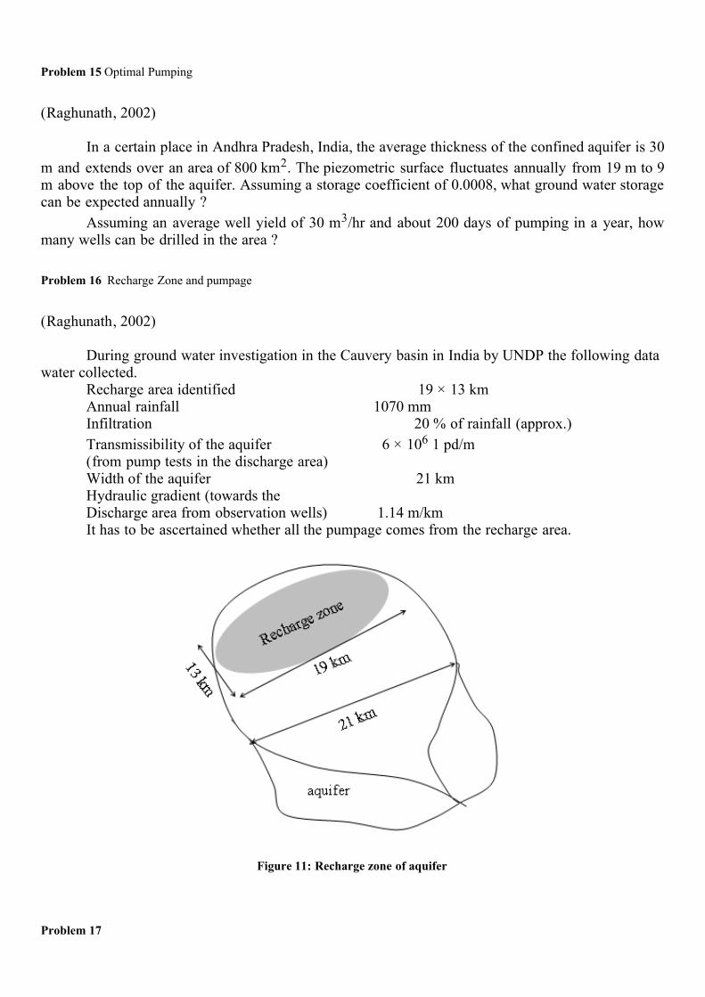
During ground water investigation in the Cauvery basin in India by UNDP the following datawater collected. Recharge area identified 19 ! 13 km Annual rainfall 1070 mm Infiltration 20 % of rainfall (approx.)

Transmissibility of the aquifer 6 ! 106 1 pd/m (from pump tests in the discharge area) Width of the aquifer 21 km Hydraulic gradient (towards the Discharge area from observation wells) 1.14 m/km It has to be ascertained whether all the pumpage comes from the recharge area.

Figure 11: Recharge zone of aquifer

Problem 17

(Raghunath, 2002)

An aquifer has an average thickness of 60 m and an aerial extent of 100 ha. Estimate theavailable ground water storage if

(a) the aquifer is unconfined and the fluctuation in GWT is observed as 15 m,(b) the aquifer is confined, and the piezometric head is lowered by 50 , which drains half

the thickness of the aquifer.

Assume a storage coefficient of 2 ! 10-4 and a specific yield of 16 %.

Problem 18

(Raghunath, 2002)

An artesian aquifer 20 m thick has a porosity of 20 % and bulk modulus of compression 108

N/m2 . Estimate the storage coefficient of the aquifer. What fraction of this is attributable to theexpansibility of water. vii) Well drawdowns

The subject of well hydraulics deals with the changes in groundwater flow caused by pumping. Foridealized assumptions, some computable functions are available to estimate the drawdown due topumping from a well. Most of these functions assume an infinite aquifer horizontally and uniformaquifer properties. Also, the impact of multiple wells can be linearly superposed. The basic work on unconfined aquifer was initiated by Dupuit in 1848 who gave the equation fordrawdown due to pumping from a well. This was later modified by Theim in 1906 to give:

Equation 9

where two points on the cone of depression at radial distances r2 and r1 have heads h2 and h1

respectively and that steady state condition of water tables is reached under constant pumping at rateQ in a medium of hydraulic conductivity K. For similar assumptions, a confined aquifer would give,

where b is thickness of the confined aquifer. This equations assume complete penetration of the wellwithin the aquifer.

Problem 19

(Karanth, 1987)

A well in the centre of an unconfined island aquifer, bounded externally by a circle of radius

1200 m, is proposed to be pumped at a rate that will limit the drawdown to 6 m at a distance of 15 mfrom the well. What should be the maximum allowable discharge of the well, given that the height ofthe static water table above the impermeable base of the aquifer is 10 m and the hydraulicconductivity of the aquifer is 0.1 m/day.

Problem 20

(Karanth, 1987) A fully penetrating well of diameter 0.30 m abstracts water from a confined aquifer. Computethe discharge when the steady state drawdown at distances of 10 and 60 m are respectively 2.4 m and0.5 m, given the thickness of the aquifer and hydraulic conductivity as 20 m and 10 m/dayrespectively. viii) Interpreting head data

Much information can be derived by interpretation of well head levels if they are understoodproperly. The patterns in spatial and temporal head levels are a product of various factors,i) geological heterogeneity, ii) aquifer thickness, iii) leaking into other aquifers, iii) pumping,recharge and discharge. From Darcy’s law, one can infer that if velocity of flow is constant, then the only factor affectinghydraulic gradient and therefore spacing of head contour should be changes in conductivity. This isso in case there is no discharge or recharge within the system and only flow from one point toanother. Often, precautions need to be taken in case of interpretation of piezometric levels towards measuringhydraulic head. The piezometric level coincides with the water table for an unconfined aquifer onlywhen the flow is almost horizontal. Sometimes, local effects such as surface water bodies couldproduce local flow systems which can be misinterpreted. Therefore, one needs to look for differentcausing factors apart from the major ones such as topography and geology. In highly forestedenvironments, there could be diurnal variations in the water table caused because of daytime ET.Such effects need to be taken into account. In human modified environments, pumping can be asignificant factor and the flow system in many cases can never be assumed to be in a steady state.One important factor when correlating piezometric levels obtained from wells in about ensuring thatthey belong to the same flow system eq. the same aquifer. Often, there is mixing of data fromdifferent aquifers leading to confusion in flow behaviour.

Problem 21 Impact of heterogeneity on head contours

(Domenico and Schwartz, 1990)

If the hydraulic conductivity in area A is 10-6 m/sec, determine the hydraulic conductivity inthe other areas. Assume the medium is isotropic and nonhomogeneous and that no flow is added to orlost from the system; that is, inflow equals outflow.

Figure 12: Flow system in heterogenous aquifer

Problem 22 Interpreting flow system from head contours

(Domenico and Schwartz, 1990) You are given the following piezometric surface:For each of the conditions cited, give one reason that can account for the piezometric surface Condition 1: Inflow across h = 80m = outflow across h = 30mCondition 2: The aquifer is homogenous and isotropicCondition 3: The aquifer is homogenous and isotropic The aquifer depicted in the Figure is underlain by a uniformly thick homogeneous clay layer.Below this clay layer is another aquifer. The head in this lower aquifer near the 70-m equipotentialline is 60m, or 10m lower than the measured 70-m equipotential line. In the vicinity of the 30-mequipotential line, the head in the lower aquifer is on the order of 25 m, or 5 m lower than themeasured 30-m equipotential line. In which of these two regions is the velocity of vertical movementacross the clay layer the greatest and why? Which way is the flow directed, upward or downward?

Figure 13: Expanding flow contours

3. Computer Exercises

3.1 Homogenous medium with reclining water table

Figure 14: Steady state flow across unconfined aquifer with homogenous properties

An gently sloping watershed slopes from West to East direction. These two barriers can beconsidered as no-flow boundaries and the only discharge point for this flow system is the springlocated in the Eastern boundary from which all discharge occurs. For simplicity consider the depositsbetween the barriers to be homogenous with uniform and isotropic properties of hydraulic

conductivity 2e-5 m/s and porosity 20%. The cross-section profile of the water table in theunconfined aquifer is shown in the Figure. Assume that the flow is bounded at the bottom of thisaquifer by an impermeable granite layer with negligible flow through the granite. Use programTopoDrive to check your results. Use 50 x 50 discretization. With model domain length of 50 m andvertical exaggeration of 10.0. Draw water table from 2m to 1m. i) Draw the steady state groundwater flow profile through this intermontane valley deposit.ii) What is the maximum travel time taken for any recharge from the high mountains on the West toreach the spring as discharge? (Hint the animation tool in the program TopoDrive to observemovement of particles starting from West towards East). If we were to observe the spring discharges,can we assume an annual cycle of recharge and discharge in this intermontane deposit?iii) Calculate the discharge across the central cross-section. Assume for this purpose, uniformgradient across the cross-section. Assume that this discharge occurs finally along the stream. Whatis the recharge rate across 1m thickness of the aquifer and 1m length of this cross-section. If therecharge coefficient is 0.25, what is the average annual rainfall of this location. If a 1 kilometrecross-section of this aquifer finally discharges through this stream, how many families can thisspring system conveniently support? (Assume 120 litres daily requirement for individual). Cross-check these flow patterns with those produced by TopoDrive program.

3.2 Heterogenous medium with reclining water table

Now insert a flow barrier of low conductivity 1e-9 m/s as below:

Figure 2: Steady state flow across unconfined aquifer with heterogenous properties

i) Draw the flow paths for this system. Which are the regions with major changes from before?ii) What is the travel time for the flow paths traversing through the base of the deposits?

Can we now consider this system as an annual cycle of recharge and discharge? How muchproportion of the discharge from the spring has actually recharged more than a year back? In thiscase, how would the recharge rate in the Western mountains be affected? What does this imply forthe number of families this spring system can sustain?

3.3 Two dimensional flow with constant head boundary conditions

Flow occurs between two lakes through an aquifer connecting them that is bounded for flowon all other sides. We consider two-dimensional flow between the two lakes through thisaquifer. The level difference between the two lakes is 50 m. Let the aquifer material be homogenous with conductivity of 0.001m/s and porosity 20%.Calculate the travel time of flow from one lake to another. Check this travel time using theprogram ParticleFlow.Now, let the aquifer have layered bands of different conductivity as shown in the Figure.Compute the effective conductivity of this combination. Use program Particle flow and alsoexpression for effective conductivity for flow in series. Now, calculate how much time it takesto travel from one lake to another.Instead, let the bands be along the flow direction, see Figure. Now, compute the effectiveconductivity again. How would you use the travel times obtained from Particle flow tocompute this same effective conductivity for this combination.A non-diffusive tracer released uniformly from the first lake is observed at the second lake toreach in spikes as shown in the figure. If porosity is uniform at 20%, guess one possibleconfiguration of hydraulic conductivity pattern within the aquifer using this tracer result. Canthere be other possibilities?

4. Solutions to Numerical problems

Problem 1

a)

Day Rainfall Soil Moisture Actual ET

Moisture

surplus

1 mm mm mm mm

2 0 100.1 4.3 0

3 45 95.8 6 0

4 26 134.8 6.4 4.4

5 19 150 6.4 12.6

6 19 150 6.4 12.6

7 26 150 6.4 19.6

8 0 150 6.4 0

Time Year Recharge fromDirectPrecipitation

m3

NetRechargefrom Stream

flow m3

Discharge by

Pumping m3

Discharge byEvapotranspiration

m3

Change inGroundWater

Storage m3

1 3 ! 107 0 0 3 ! 107 0

2 3 ! 107 6 ! 105 1 ! 107 3 ! 107 94 ! 105

: : : : : :

7 3 ! 107 1 ! 106 3 ! 107 9 ! 106 8 ! 106

8 2.8 ! 107 2 ! 106 3.5 ! 107 5 ! 106 10 ! 106

9 2.5 ! 107 3 ! 106 3.5 ! 107 3 ! 106 10 ! 106

10 3.5 ! 107 4 ! 106 4 ! 107 1 ! 106 2 ! 106

11 3.5 ! 107 4 ! 106 4.2 ! 107 1 ! 106 4 ! 106

12 3.5 ! 107 4 ! 106 4 ! 107 1 ! 106 2 ! 106

The abstraction from this aquifer exceeds the long term average recharge by 4.5 x 106 m3. Thereforeone can say that the current abstraction is reducing the storage of the aquifer. This might result indifferent adverse consequences such as increase in energy for pumping, greater investment for wells,drying up of wells, increased mineralization of groundwater etc. All these together would determinethe degree of overexploitation of the aquifer. b) The proportion of natural recharge available for natural ET changes over the years as 100%, 98%,29%, 16.7%, 10.7%, 2.6%, 2.6% and 2.6%. All the recharge is now being diverted for pumping. c) The decline in water levels over the years are 0 m, 9.4 m, 8 m, 10 m, 10 m , 2 m , 4 m , 2 m, i.ean average of 5.6 m every year. This is a rapid decline of water level conditions.

d) In year 8, the net overabstraction is 2 x 106 m3. The pumping would need to be limited to 40-2 =

38 x 106 m3 so that the water level is steady. This however does not change the water available fornatural ET which will still be low. Problem 2

Table 5

a)

Rainfall = Actualevapotranspiration + Moisturesurplus ± Change in soil Moisturestorage (Remaining

soil moisture – Antecedent soil moisture) 135.0 = 42.3 + 49.2 + 43.5 b) The total moisture surplus is 43.5 mm. If 20% of this infiltrates, then the recharge to groundwater

is 0.2*43.5 = 8.7 mm. The rainfall-recharge coefficient is therefore 8.7 mm out of 135 mm storm i.e.6.4%. Problem 3

Applying the expression we get the following: Depth of piezo (ft): 600, 575, 150, 25Total head (ft): 900, 800, 700, 600Pressure head (ft): 600, 575, 150, 25Elevation Head(ft): 300, 225, 550, 575 Problem 4

Head1 = Elevation head + Pressure head = 50 cm + 32 cm = 82 cmHead2 = Elevation head + Pressure head = 30 cm + 26 cm = 56 cm

Q = kiA = 10m/day * (82-56)/50 * p*(0.1)2 = 0.163 m3/day

Problem 5

Soln: From Darcy’s law,

Hydraulic gradient

= = 12/1800 = 6.67! 10-4

v = 0.073 m/day Problem 6

It has taken 20,000 years for the ground water movement through the inclined water bearingstratum, to form a recent potential ground water storage.

v = = m/d Applying Darcy’s law,

0.00438 = K K = 21.90 m/day Transmissibility of the water bearing stratum,

T = K. b = 21.90 ! 30

= 657 m2/day or m3/day/m

= 657,000 1pd/m, or 657 m2/day.

Problem 7

Soln: The flow required is 10,000 x 20 x 10-3 m3 / day i.e. 200 m3 / day

The velocity through this sand is v = K . I = 2 ! 10-5 m/sec x 0.7/0.3 m/sec = 4.032 m/day

A = Q/v = 200 / 4.032 = 49.6 m2 of area required i.e. a 7 m x 7 m area pit with depth of 0.3 m Problem 8

Soln: Effective conductivity for flow in horizontal direction is:(5 x 12 + 10 x 25 + 10 x 40)/(5 + 10 + 10) = 28.4 m/d

Q = KIA = 28.4m/d * 1/300 * 1000 m = 94.67 m3/d At the rate of 200 litres per household, we can accomodate 473 households. The distance traveled by this flow in 1 day is 28.4 * 1/300 = 9.5 cm. In 365 days, it would travel,34.55 metres. Assuming that the output water is discharged after 1 year, one can flush out the wastewater through this system. However, note that the input water would create a new head gradient andalter the previous flow. So in actual, the bed system would need to be longer. This can be determinedby solving for a constant flow boundary in a confined aquifer system. Problem 9

18/K = 15/1.2 + 3/0.08 K = 0.36 m/dayi = 2/18 = 1/9v = Ki = 4 cm/day Problem 10

Soln:qleak = K (h1 – h2)/h2 = 1.2 * (20 – 12)/12 = 0.8 m/day

The vertical hydraulic gradient is (20-12)/12 = 0.667 m/m. For a point 3 m above top of the arterianaquifer, the head drop will be 3*2/3 = 2m, i.e. at 2m below ground level. Problem 11

Soln: Water drained = Area * Water level fall * Specific Yield. The water drains through two layerswith different specific yields of (25% - 5% = 20%) and (22% - 10% = 12%) respectively. The totalwater drained = 1sq. km. * 0.8 m * 0.2 + 1sq. km. * 1.2 m * 0.12 = 0.16 sq. km. m + 0.144 sq.km. m= 0.304 sq. km. m. = 0.304 MCM. The proportion of base flow is 60%. Problem 12

Problem 12

Q = A. Sy . H

1.5 * 106 = 50 * 106 . Sy . 2Sy = 0.15 Rf = H. Sy /R = 0.2

An additional recharge of 0.375 * 106 m3 is aimed, This needs a runoff of 1.25 * 106 m3. for arainfall of 800 mm, a catchment area of 156.25 hectares are needed.

Problem 13

a) From the graph, the minimum rainfall required for rise in water level is around 0.3 m, 300 mm.This is true for several arid areas with deep water table.b) Average water table fluctuation is 0.92 m from 1980 till 1984.c) Average recharge is 0.34 m from 1980 till 1984.d) Taking the rainfall-infiltration each year and taking average of that we get, average rainfallinfiltration factor is 35%..

Total annual domestic water requirement/km2 = 120 l * 350 *365 = 15330 m3. The irrigation water

requirement is 153300 m3. The rainfall needed to affect this recharge is (153300 + 15330)*100/35 =

481800 m3. With an average annual rainfall of 800 mm, this requires a catchment runoff generation

area of 6.02 km2. This means that the population over each piece of land is utilizing groundwater recharge generatedover 6 times as much an area.

Problem 14

Solution:Volume of water pumped out = Area of aquifer ! drop in g.w.t. ! specific yield

3 ! 105 = 106 ! 2.2 ! Sy

Sy = 0.136, or 13.6 %

Volume of irrigation water recharging the aquifer = Area of aquifer ! rise in g.w.t. ! Sy

Considering an area of 1 m2 of aquifer, 1 ! y = 1 ! 1 ! 0.136Recharge volume (depth) y = 0.136 m, or 136 mmSoil moisture deficit (below field capacity ) before irrigation = 200-136 = 64 mmProblem 15

Solution:"GWS = Aaq ! "piezo. Surface ! S = (800 ! 106 )(19-9) 0.0008

Or 6.4-106 m3, or 6.4 m3

Annual draft = (30 ! 24) 200 = 0.144 ! 106 m3

Number of wells that can be drilled in the area = 6.4 --- 0.144 = 44.5, say 44 wellsof course, the well sites have to be investigated and these should be sufficient spacing for the wells. Problem 16

Solution: 20

Annual recharge = (19 ! 13) 106 --------- ! 1.07 = 5.29 ! 107 m3

100 1.14

Q = Tiw = (6 ! 103) ------ ! 21,000 1000

= 144 ! 103 m3/day

Annual pumpage = (144 ! 103) 365 = 5.25 ! 107 m3

Thus the entire pumpage comes from the recharge area.. Problem 17

Solution: (a) "GWS = Aaq . "GWS. Sy = 100 ha ! 15 m (0.16)

= 240 ha-m (b) "GWS = Aaq[" piezo. Head ! S + " GWT ! SY]

(as confined) (as unconfined)

= 100 ha [20 (2!10-4) + 30 (0.16)] = 480 Problem 18

Solution: S = !wb (" + n#)

1 1 = 9810 $ 20 (--- + 0.20 $ ---------)

108 2.1$ 109

= (1.962 + 0.0187) 10-3

= 1.98 $ 10-3 , say, 2 $ 10-3

The fraction of storage attributable to the expansibility of water (taking only the second termwithin the brackets)

Sw = 0.0187 $ 10-3

1.87 $ 10-5

= -------------- of S

1.98 $ 10-3 1

» ----- of S, or 1 % of S

100 Problem 19

Soln: Applying Theim equation for unconfined aquifers:

Q = pK(h22 – h

21)/(2.3 log(r2/r1) = 6.03 m3/day

Problem 20

Applying Theim equation for confined aquifers:

Q = 2pKb(s1 – s2)/(2.3 log(r2/r1) ) = 1334 m3/day

Problem 21

In region B, the equipotential lines are spaced similarly apart as in region A, therefore,K1i1 = K2i2 gives the same K i.e. 10-6 m/s. For region C, the equipotential lines are spaced half as

wide as in region A, thereore the gradient is half slower, making K twice i.e. 2 x 10-6 m/s. In regionD, the equipotential lines are spaced twice closer as in region A, making the gradient twice faster, the

K therefore is 5 x 10-7 m/s. Problem 22

Condition 1: If the inflow and outflows are the same and the aquifer thickness is also the same, thenthe cause for hydraulic gradient decreasing towards right should be because of increasing hydraulicconductivity in that direction Condition 2: If the aquifer is homogenous and isotropic, then we could have one case where inflowis not equal to outflow. In that case decrease in hydraulic gradient could be due to leakage from theaquifer, maybe to a lower aquifer

Condition 3: In this case, we can consider the aquifer thickness to be increasing from left to right,therefore causing a decrease in rate of flow, therefore, hydraulic gradient. The vertical hydraulic gradient is greater (10m) at the 70-m equipotential line than at the 30-mequipotential line (5m). Therefore assume other properties such as aquifer properties and clayproperties to be similar, we can deduct that the rate of vertical leakage is downward and greater at the70-m equipotential line.

5. Solutions to Computer Exercises

Solution to 3.1

Taking a 50 x 50 discretization. ii) Approx in 360 days, most of the discharge has occurred. Yes, for practical purpose, we canconsider this system as recharging and discharging annually. iii) Assume that the flow gradient of (2-1)/50 i.e. 0.02 m/m is present at the central cross-section

with vertical area of 1.5m2.

q = kiA = 2e-5 * (2-1)/50 * 1.5 m3 / s for 1 metre of thickness

= 6e-7 m3 / s for 1 metre of thickness. = 6e-4 litres/s.The total recharge per unit length across this cross-section with 1m thickness contributing to this

flow is 6e-7/50m = 12e-6mm/m2/s. This corresponds to 1.02 mm/m2/day of recharge per unit area.If the recharge coefficient is 0.25 the average rainfall contributing to this recharge is 1.02/0.25 = 4.08mm/day which comes to 1489 mm average annual rainfall. Taking 120 lpcd as the water requirement/person, we have 600 litres of daily requirement for afamily of 5. The total discharge per day is 6e-4*60*60*24 = 51.84 litres/metre thickness/day. For akilometer long thickness, it can support 51.84*1000*/120 = 432 families. Solution to 3.2

i)

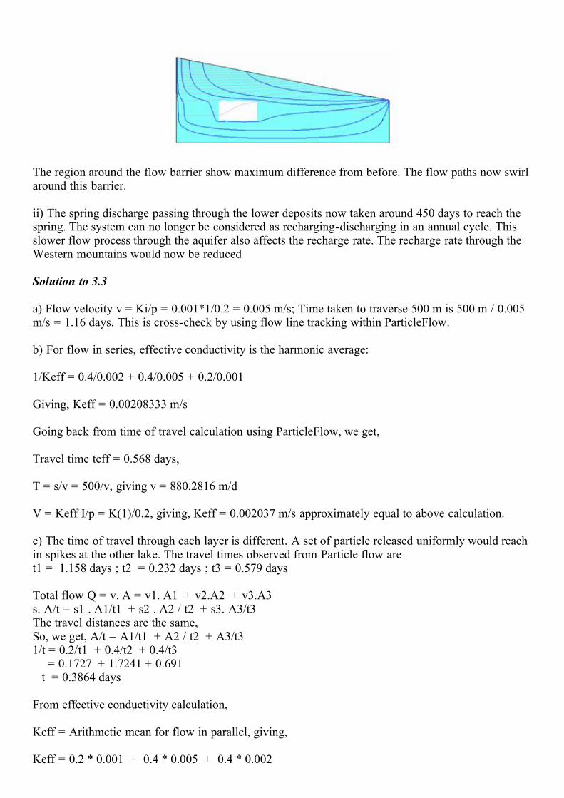
The region around the flow barrier show maximum difference from before. The flow paths now swirlaround this barrier. ii) The spring discharge passing through the lower deposits now taken around 450 days to reach thespring. The system can no longer be considered as recharging-discharging in an annual cycle. Thisslower flow process through the aquifer also affects the recharge rate. The recharge rate through theWestern mountains would now be reduced Solution to 3.3

a) Flow velocity v = Ki/p = 0.001*1/0.2 = 0.005 m/s; Time taken to traverse 500 m is 500 m / 0.005m/s = 1.16 days. This is cross-check by using flow line tracking within ParticleFlow. b) For flow in series, effective conductivity is the harmonic average: 1/Keff = 0.4/0.002 + 0.4/0.005 + 0.2/0.001 Giving, Keff = 0.00208333 m/s Going back from time of travel calculation using ParticleFlow, we get, Travel time teff = 0.568 days, T = s/v = 500/v, giving v = 880.2816 m/d V = Keff I/p = K(1)/0.2, giving, Keff = 0.002037 m/s approximately equal to above calculation. c) The time of travel through each layer is different. A set of particle released uniformly would reachin spikes at the other lake. The travel times observed from Particle flow aret1 = 1.158 days ; t2 = 0.232 days ; t3 = 0.579 days Total flow Q = v. A = v1. A1 + v2.A2 + v3.A3s. A/t = s1 . A1/t1 + s2 . A2 / t2 + s3. A3/t3 The travel distances are the same,So, we get, A/t = A1/t1 + A2 / t2 + A3/t3 1/t = 0.2/t1 + 0.4/t2 + 0.4/t3 = 0.1727 + 1.7241 + 0.691 t = 0.3864 days From effective conductivity calculation, Keff = Arithmetic mean for flow in parallel, giving, Keff = 0.2 * 0.001 + 0.4 * 0.005 + 0.4 * 0.002

= 0.003 m/sV = KI/p = 0.015 m/s T = s/V = 0.3858 days, approximately equal to calculation from ParticleFlow d) The tracer arrives in spikes as in the example in c). Therefore, there must be parallel layers withdifferent conductivities. The travel time for arrival are:t1 = 0.24 days, t2 = 1.16 days and t3 = 0.58 days, giving velocities ofv1 = 0.02411 m/s, 0.004989 m/s and v3 = 0.009978 m/s respectively.The conductivies are:K1 = 0.00488 approx 0.005 m/sK2 = 0.0009978 approx 0.001 m/sK3 = 0.0019955 m/s, approx, 0.002m/s Each of thickness, T1 = 100 m, T2 = 200 m and T3 = 200 m. These can be ordered in any particularfashion, i.e. they could be divided into as many parts and interspersed between each other. It onlymatters that they are aligned in parallel finally, but their orientiation in North-South cannot bedetermined from this data alone.

6. References

Karanth, K. R., 1987, Groundwater assessment, development and management, Tata-McGraw HillPublishing Company Limited, New Delhi Hillel D., 1998, Environmental Soil Physics, Academic Press Domenico A. A. and F. W. Schwartz, 1990, Physical and Chemical Hydrogeology, John Wiley andSons Hsieh, P.A., 2001, TopoDrive and ParticleFlow—Two Computer Models for Simulation andVisualization of Ground-Water Flow and Transport of Fluid Particles in Two Dimensions: U.S.Geological Survey Open-File Report 01-286, 30 p Raghunath, H. M., 2002, Groundwater, New Age International Publishers, New Delhi

7. Instructions and links for Softwares

The softwares TopoDrive and ParticleFlow for use in the exercises and their documentation areavailable at: http://water.usgs.gov/nrp/gwsoftware/tdpf/tdpf.html