an epr primer 2 - iowa state university epr... · xenon user’s guide an epr primer 2 this chapter...

Xenon User’s Guide

An EPR Primer 2

This chapter is an introduction to the basic theory and practice of EPR spec-troscopy. It gives you sufficient background to understand the followingchapters. In addition, we strongly encourage the new user to explore some ofthe texts and articles at the end of this chapter. You can then fully benefitfrom your particular EPR application or think of new ones.

Basic EPR Theory 2.1

Introduction to Spectroscopy 2.1.1During the early part of the 20th century, when scientists began to apply theprinciples of quantum mechanics to describe atoms or molecules, they foundthat a molecule or atom has discrete (or separate) states, each with a corre-sponding energy. Spectroscopy is the measurement and interpretation of theenergy differences between the atomic or molecular states. With knowledgeof these energy differences, you gain insight into the identity, structure, anddynamics of the sample under study.

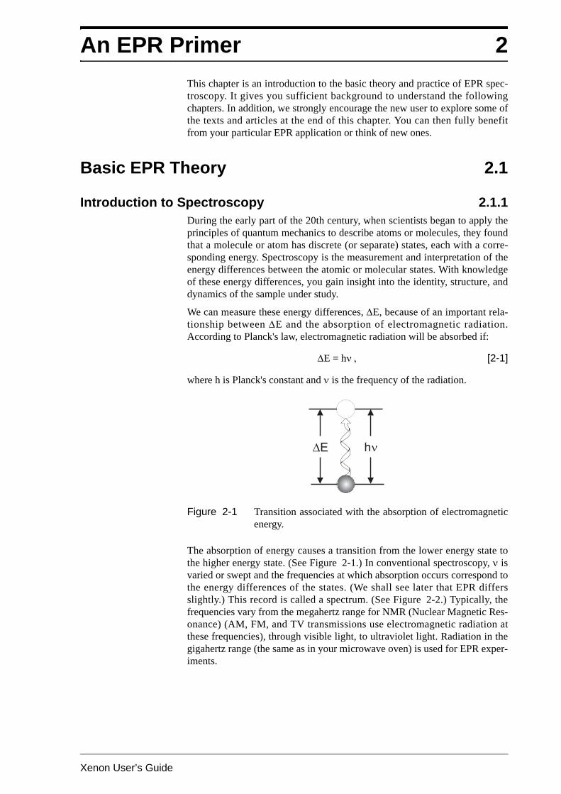
We can measure these energy differences, E, because of an important rela-tionship between E and the absorption of electromagnetic radiation.According to Planck's law, electromagnetic radiation will be absorbed if:

E = h [2-1]

where h is Planck's constant and is the frequency of the radiation.

The absorption of energy causes a transition from the lower energy state tothe higher energy state. (See Figure 2-1.) In conventional spectroscopy, isvaried or swept and the frequencies at which absorption occurs correspond tothe energy differences of the states. (We shall see later that EPR differsslightly.) This record is called a spectrum. (See Figure 2-2.) Typically, thefrequencies vary from the megahertz range for NMR (Nuclear Magnetic Res-onance) (AM, FM, and TV transmissions use electromagnetic radiation atthese frequencies), through visible light, to ultraviolet light. Radiation in thegigahertz range (the same as in your microwave oven) is used for EPR exper-iments.

Figure 2-1 Transition associated with the absorption of electromagneticenergy.

�E h�

Basic EPR Theory

2-2

The Zeeman Effect 2.1.2The energy differences we study in EPR spectroscopy are predominately dueto the interaction of unpaired electrons in the sample with a magnetic fieldproduced by a magnet in the laboratory. This effect is called the Zeemaneffect. Because the electron has a magnetic moment, it acts like a compass ora bar magnet when you place it in a magnetic field, B0. It will have a state oflowest energy when the moment of the electron, µ, is aligned with the mag-netic field and a state of highest energy when µ is aligned against the mag-netic field. (See Figure 2-3.) The two states are labelled by the projection ofthe electron spin, Ms, on the direction of the magnetic field. Because the elec-tron is a spin 1/2 particle, the parallel state is designated as Ms = - 1/2 and theantiparallel state is Ms = + 1/2.

From quantum mechanics, we obtain the most basic equations of EPR:

E = g B B0 Ms = ± g B B0 [2-2]

and

E = h = g BB0. [2-3]

Figure 2-2 A spectrum.

h1 h2

1 2

Absorption

Figure 2-3 Minimum and maximum energy orientations of µ withrespect to the magnetic field B0.

B0B0

12---

Basic EPR Theory

Xenon User’s Guide 2-3

g is the g-factor, which is a proportionality constant approximately equal to 2for most samples, but varies depending on the electronic configuration of theradical or ion. µB is the Bohr magneton, which is the natural unit of electronicmagnetic moment.

Two facts are apparent from equations Equation [2-2] and Equation [2-3] andits graph in Figure 2-4.

• The two spin states have the same energy in the absence of a magneticfield.

• The energies of the spin states diverge linearly as the magnetic fieldincreases. For g = 2, the slope is 2.8 MHz/G.

These two facts have important consequences for spectroscopy.

• Without a magnetic field, there is no energy difference to measure.

• The measured energy difference depends linearly on the magnetic field.

Because we can change the energy differences between the two spin states byvarying the magnetic field strength, we have an alternative means to obtainspectra. We could apply a constant magnetic field and scan the frequency ofthe electromagnetic radiation as in conventional spectroscopy. Alternatively,we could keep the electromagnetic radiation frequency constant and scan themagnetic field. (See Figure 2-4.) A peak in the absorption will occur whenthe magnetic field “tunes” the two spin states so that their energy differencematches the energy of the radiation. This field is called the “field for reso-nance”. Owing to the limitations of microwave electronics, the latter methodoffers superior performance. This technique is used in all Bruker EPR spec-trometers.

The field for resonance is not a unique “fingerprint” for identification of acompound because spectra can be acquired at several different frequencies.The g-factor,

[2-4]

Figure 2-4 Variation of the spin state energies as a function of theapplied magnetic field.

B0

Absorption

E

g hBB0-------------=

Basic EPR Theory

2-4

being independent of the microwave frequency, is much better for that pur-pose. Notice that high values of g occur at low magnetic fields and vice versa.A list of fields for resonance for a g = 2 signal at microwave frequenciescommonly available in EPR spectrometers is presented in Table 2-1.

Hyperfine Interactions 2.1.3Measurement of g-factors can give us some useful information; however, itdoes not tell us much about the molecular structure of our sample. Fortu-nately, the unpaired electron, which gives us the EPR spectrum, is very sensi-tive to its local surroundings. The nuclei of the atoms in a molecule orcomplex often have a magnetic moment, which produces a local magneticfield at the electron. The interaction between the electron and the nuclei iscalled the hyperfine interaction. It gives us a wealth of information about oursample such as the identity and number of atoms which make up a radical orcomplex as well as their distances from the unpaired electron.

Figure 2-5 depicts the origin of the hyperfine interaction. The magneticmoment of the nucleus acts like a bar magnet (albeit a weaker magnet thanthe electron) and produces a magnetic field at the electron, BI. This magnetic

Microwave Band Frequency (GHz) Bres (G)

L 1.1 390

S 4.0 1430

X 9.75 3480

Q 34.0 12100

W 94.0 33500

Table 2-1 Field for resonance, Bres, for a g = 2 signal at selected microwave frequencies.

Figure 2-5 Local magnetic field at the electron, BI, due to a nearbynucleus.

B0

Electron

B0

BI

BI

Electron

Nucleus

Nucleus

Basic EPR Theory


field opposes or adds to the magnetic field from the laboratory magnet,depending on the alignment of the moment of the nucleus. When BI adds tothe magnetic field, we need less magnetic field from our laboratory magnetand therefore the field for resonance is lowered by BI. The opposite is truewhen BI opposes the laboratory field.

For a spin 1/2 nucleus such as a hydrogen nucleus (proton), we observe thatour single EPR absorption signal splits into two signals which are each BIaway from the original signal. (See Figure 2-6.)

For nuclei with spins other than 1/2, the number of lines equals:

[2-5]

where I is the spin quantum number of the nucleus.

If there are two spin 1/2 nuclei with the same hyperfine coupling, each of thetwo lines is further split into two lines. Because of the equal hyperfine cou-

Figure 2-6 Splitting in an EPR signal due to the local magnetic field of anearby nucleus.

Figure 2-7 The number of lines from hyperfine interactions increases as2I+1 with the nuclear spin quantum number, I.

BI BI

Number of Lines 2I 1+=

Hydrogen I = 1/2

Nitrogen I = 1

Manganese I = 5/2

Basic EPR Theory

2-6

pling two of the EPR signals will overlap, giving a triplet with an intensitydistribution of 1:2:1.

For n spin 1/2 nuclei with equal hyperfine couplings, the number of lines isgiven by:

[2-6]

with each of the lines separated by the hyperfine coupling. The relative inten-sities are given by:

[2-7]

which are related to Pascal’s triangle and polynomial coefficients.

Figure 2-8 A 1:2:1 triplet resulting from the hyperfine interactions oftwo equivalent spin 1/2 nuclei.

1

2

1

BI

BI

BI

Number of Lines 2n 1+=

n

k n!

k! n k– !------------------------= 0 k n

Figure 2-9 Relative intensities for benzosemiquinone (a) and durosemiquinone (b) radical anionsin alkaline DMSO. The number of lines is given by Equation [2-6] and the relativeintensities by Equation [2-7].

O O

O O

H Me

H Me

H Me

H Me

1 1

4 4

6 924

495495

2202206666 1212 11

792792

a) b)

Basic EPR Theory


The situation for nuclei with different hyperfine couplings is similar to equalhyperfine couplings, except that there is no overlap between the lines leadingto the Pascal triangle intensity distribution. Each of the lines is split by theadditional hyperfine couplings.

As an example, it is possible to make the durosemiquinone radical cation.This is similar to the anion shown in Figure 2-9 except that the oxygens areprotonated, thus producing further hyperfine splittings. We start off on the leftside of Figure 2-10 with the 13 line pattern to be expected from the 12 equiv-alent methyl protons. Then there is the additional splittings from the hydro-gens bound to the oxygens. Since the two protons are equivalent, we have a1:2:1 triplet from them. If we split each of the 13 lines from the methyl protonsplittings with this 1:2:1 triplet, we see that we can nicely reproduce the com-plicated experimental EPR spectrum of the durosemiquinone radical cation insulfuric acid.

For N spin 1/2 nuclei, we will generally observe 2N EPR signals. As the num-ber of nuclei gets larger, the number of signals increases exponentially. Some-times there are so many signals that they overlap and we only observe onebroad signal, resulting in what is called a gaussian lineshape.

Figure 2-10 Estimating the EPR spectrum of the durosemiquinone radical cation in sulfuric acidand reduced with sodium dithionite by splitting each of the EPR lines due to the 12methyl protons by a 1:2:1 triplet from the hydroxyl protons.

O

O

Me

Me

Me

Me

H

H

12 Methyl Protons Two Hydroxyl Protons

Figure 2-11 A large number of nuclei produces a gaussian lineshape.

Basic EPR Practice

2-8

Signal Intensity 2.1.4So far, we have concerned ourselves with the field for resonance of the EPRsignal, but the size of the EPR signal is also important if we want to measurethe concentration of the EPR active species in our sample. In the language ofspectroscopy, the size of a signal is defined as the integrated intensity, i.e., thearea beneath the absorption curve. (See Figure 2-12.) The integrated inten-sity of an EPR signal is proportional to the concentration.

Signal intensities do not depend solely on concentrations. They also dependon the microwave power. If you do not use too much microwave power, thesignal intensity grows as the square root of the power. At higher power levels,the signal diminishes as well as broadens with increasing microwave powerlevels. This effect is called saturation. If you want to measure accurate line-widths, lineshapes, and closely spaced hyperfine splittings, you should avoidsaturation by using low microwave power. A quick means of checking for theabsence of saturation is to decrease the microwave power and verify that thesignal intensity also decreases by the square root of the microwave power.

Some of these topics are covered in greater detail in Section 2.7.

Basic EPR Practice 2.2

Introduction to Spectrometers 2.2.1In the first half of this chapter, we discussed the theory of EPR spectroscopy.Now we need to consider the practical aspects of EPR spectroscopy. Theoryand practice have always been strongly interdependent in the developmentand growth of EPR. A good example of this point is the first detection of anEPR signal by Zavoisky in 1945. The Zeeman effect had been known in opti-cal spectroscopy for many years, but the first direct detection of EPR had towait until the development of radar during World War II. Only then, did sci-entists have the necessary components to build sufficiently sensitive spec-trometers (scientific instruments designed to acquire spectra). The same istrue today with the development of advanced techniques in EPR such as Fou-rier Transform and high frequency EPR.

The simplest possible spectrometer has three essential components: a sourceof electromagnetic radiation, a sample, and a detector. (See Figure 2-13.) Toacquire a spectrum, we change the frequency of the electromagnetic radiationand measure the amount of radiation which passes through the sample with adetector to observe the spectroscopic absorptions. Despite the apparent com-plexities of any spectrometer you may encounter, it can always be simplifiedto the block diagram shown in Figure 2-13.

Figure 2-12 Integrated intensity of absorption signals. Both signals havethe same intensity.

Basic EPR Practice


Figure 2-14 shows the general layout of a Bruker EPR spectrometer. Theelectromagnetic radiation source and the detector are in a box called the“microwave bridge”. The sample is in a microwave resonator (or cavity),which is a metal box that helps to amplify weak signals from the sample. Asmentioned in Section 2.1.2, there is a magnet to “tune” the electronic energylevels. In addition, we have a console, which contains signal processing andcontrol electronics. There is a computer used for analyzing data as well ascoordinating all the units for acquiring a spectrum. In the following sectionsyou will become acquainted with how these different parts of the spectrome-ter function and interact.

Figure 2-13 The simplest spectrometer.

Source Sample Detector

Figure 2-14 The modules and components of the EMXplus spectrometer.

EMXplus

EMXpremiumX

MicrowaveBridge

Console Magnet

MagnetPowerSupply

Resonator LinuxWorkstation

Basic EPR Practice

2-10

The Microwave Bridge 2.2.2The microwave bridge houses the microwave source and the detector. Thereare more parts in a bridge than shown in Figure 2-15, but most of them arecontrol, power supply, and security electronics and are not necessary forunderstanding the basic operation of the bridge. We shall now follow the pathof the microwaves from the source to the detector.

We start our tour of the microwave bridge at point A, the microwave source.The output power of the microwave source cannot be varied easily, howeverin our discussion of signal intensity, we stressed the importance of changingthe power level. Therefore, the next component, at point B, after the micro-wave source is a variable attenuator, a device which blocks the flow of micro-wave radiation. With the attenuator, we can precisely and accurately controlthe microwave power which the sample sees.

Bruker EPR spectrometers operate slightly differently than the simple spec-trometer shown in the block diagram, Figure 2-13. The diagram depicts atransmission spectrometer (It measures the amount of radiation transmittedthrough the sample.) and most EPR spectrometers are reflection spectrome-ters. They measure the changes (due to spectroscopic transitions) in theamount of radiation reflected back from the microwave cavity containing thesample (point D in the Figure 2-15). We therefore want our detector to seeonly the microwave radiation coming back from the cavity. The circulator at

Figure 2-15 Block diagram of a microwave bridge.

A

B

C

D

E

F

G

Source

ReferenceArm

Cavity

Attenuator

SignalOut

DetectorDiode

Circulator

Basic EPR Practice


point C is a microwave device which allows us to do this. Microwaves com-ing in port 1 of the circulator only go to the cavity through port 2 and notdirectly to the detector through port 3. Reflected microwaves are directedonly to the detector and not back to the microwave source.

We use a detector diode to detect the reflected microwaves (point E inFigure 2-15). It converts the microwave power to an electrical current. Atlow power levels, (less than 1 microwatt) the diode current is proportional tothe microwave power and the detector is called a square law detector.(Remember that electrical power is proportional to the square of the voltageor current.) At higher power levels, (greater than 1 milliwatt) the diode cur-rent is proportional to the square root of the microwave power and the detec-tor is called a linear detector. The transition between the two regions is verygradual.

For quantitative signal intensity measurements as well as optimal sensitivity,the diode should operate in the linear region. The best results are attainedwith a detector current of approximately 200 microamperes. To insure thatthe detector operates at that level, there is a reference arm (point F in theFigure 2-15) which supplies the detector with some extra microwave poweror “bias”. Some of the source power is tapped off into the reference arm,where a second attenuator controls the power level (and consequently thediode current) for optimal performance. There is also a phase shifter to insurethat the reference arm microwaves are in phase with the reflected signalmicrowaves when the two signals combine at the detector diode.

The detector diodes are very sensitive to damage from excessive microwavepower and will slowly lose their sensitivity. To prevent this from happening,there is protection circuitry in the bridge which monitors the current from thediode. When the current exceeds 400 microamperes, the bridge automaticallyprotects the diode by lowering the microwave power level. This reduces therisk of damage due to accidents or improper operating procedures. However,it is good lab practice to follow correct procedures and not rely on the protec-tion circuitry.

The EPR Cavity 2.2.3In this section, we shall discuss the properties of microwave (EPR) cavitiesand how changes in these properties due to absorption result in an EPR sig-nal. We use microwave cavities to amplify weak signals from the sample. Amicrowave cavity is simply a metal box with a rectangular or cylindricalshape which resonates with microwaves much as an organ pipe resonateswith sound waves. Resonance means that the cavity stores the microwaveenergy; therefore, at the resonance frequency of the cavity, no microwaveswill be reflected back, but will remain inside the cavity. (See Figure 2-16.)

Figure 2-16 Reflected microwave power from a resonant cavity.

ReflectedMicrowave

Powerres

Basic EPR Practice

2-12

Cavities are characterized by their Q or quality factor, which indicates howefficiently the cavity stores microwave energy. As Q increases, the sensitivityof the spectrometer increases. The Q factor is defined as

[2-8]

where the energy dissipated per cycle is the amount of energy lost during onemicrowave period. Energy can be lost to the side walls of the cavity becausethe microwaves generate electrical currents in the side walls of the cavitywhich in turn generates heat. We can measure Q factors easily because thereis another way of expressing Q:

[2-9]

where res is the resonant frequency of the cavity and is the width at halfheight of the resonance.

A consequence of resonance is that there will be a standing wave inside thecavity. Standing electromagnetic waves have their electric and magnetic fieldcomponents exactly out of phase, i.e. where the magnetic field is maximum,the electric field is minimum and vice versa. The spatial distribution of theamplitudes of the electric and magnetic fields in a commonly used EPR cav-ity is shown in Figure 2-17. We can use the spatial separation of the electricand magnetic fields in a cavity to great advantage. Most samples havenon-resonant absorption of the microwaves via the electric field (this is how amicrowave oven works) and the Q will be degraded by an increase in the dis-sipated energy. It is the microwave magnetic field that drives the absorptionin EPR. Therefore, if we place our sample in the electric field minimum andthe magnetic field maximum, we obtain the biggest signals and the highestsensitivity. The cavities are designed for optimal placement of the sample.

We couple the microwaves into the cavity via a hole called an iris. The size ofthe iris controls the amount of microwaves which will be reflected back fromthe cavity and how much will enter the cavity. The iris accomplishes this bycarefully matching or transforming the impedances (the resistance to thewaves) of the cavity and the waveguide (a rectangular pipe used to carrymicrowaves). There is an iris screw in front of the iris which allows us toadjust the “matching”. This adjustment can be visualized by noting that as thescrew moves up and down, it effectively changes the size of the iris. (See

Figure 2-17 Magnetic and electric field patterns in a standard EPR cavity.

Q 2 (energy stored)energy dissipated per cycle-----------------------------------------------------------------=

Qres

-------- ,=

Microwave Magnetic Field Microwave Electric Field

SampleStack

SampleStack

Basic EPR Practice


Figure 2-18.) When the iris screw properly matches the cavity impedance(also called critical coupling), no microwaves are reflected back from thecavity.

How do all of these properties of a cavity give rise to an EPR signal? Whenthe sample absorbs the microwave energy, the Q is lowered because of theincreased losses and the coupling changes because the absorbing samplechanges the impedance of the cavity. The cavity is therefore no longer criti-cally coupled and microwave will be reflected back to the bridge, resulting inan EPR signal.

The Signal Channel 2.2.4EPR spectroscopists use a technique known as phase sensitive detection toenhance the sensitivity of the spectrometer. The advantages include less noisefrom the detection diode and the elimination of baseline instabilities due tothe drift in DC electronics. A further advantage is that it encodes the EPR sig-nals to make it distinguishable from sources of noise or interference whichare almost always present in a laboratory. The signal channel, a unit whichfits in the spectrometer console, contains the required electronics for thephase sensitive detection.

The detection scheme works as follows. The magnetic field strength whichthe sample sees is modulated (varied) sinusoidally at the modulation fre-quency. If there is an EPR signal, the field modulation quickly sweepsthrough part of the signal and the microwaves reflected from the cavity areamplitude modulated at the same frequency. For an EPR signal which isapproximately linear over an interval as wide as the modulation amplitude,the EPR signal is transformed into a sine wave with an amplitude propor-tional to the slope of the signal (See Figure 2-19.)

Figure 2-18 The matching of a microwave cavity to waveguide.

IrisScrew

Wave-guide

Cavity

Iris

Figure 2-19 Field modulation and phase sensitive detection.

First Derivative

Basic EPR Practice

2-14

The signal channel (more commonly known as a lock-in amplifier or phasesensitive detector) produces a DC signal proportional to the amplitude of themodulated EPR signal. It compares the modulated signal with a reference sig-nal having the same frequency as the field modulation and it is only sensitiveto signals which have the same frequency and phase as the field modulation.Any signals which do not fulfill these requirements (i.e., noise and electricalinterference) are suppressed. To further improve the sensitivity, a time con-stant is used to filter out more of the noise.

Phase sensitive detection with magnetic field modulation can increase oursensitivity by several orders of magnitude; however, we must be careful inchoosing the appropriate modulation amplitude, frequency, and time con-stant. All three variables can distort our EPR signals and make interpretationof our results difficult.

As we apply more magnetic field modulation, the intensity of the detectedEPR signals increases; however, if the modulation amplitude is too large(larger than the linewidths of the EPR signal), the detected EPR signal broad-ens and becomes distorted. (See Figure 2-20.) A good compromise betweensignal intensity and signal distortion occurs when the amplitude of the mag-netic field modulation is equal to the width of the EPR signal. Also, if we usea modulation amplitude greater than the splitting between two EPR signals,we can no longer resolve the two signals.

Time constants filter out noise by slowing down the response time of thespectrometer. As the time constant is increased, the noise levels will drop. Ifwe choose a time constant which is too long for the rate at which we scan themagnetic field, we can distort or even filter out the very signal which we aretrying to extract from the noise. Also, the apparent field for resonance willshift. Figure 2-21 shows the distortion and disappearance of a signal as thetime constant is increased. If you need to use a long time constant to see aweak signal, you must use a slower scan rate. A safe rule of thumb is to makesure that the time needed to scan through a single EPR signal should be tentimes greater than the length of the time constant.

Figure 2-20 Signal distortions due to excessive field modulation.

Mo

du

latio

nA

mp

litu

de

B0

Basic EPR Practice


For samples with very narrow or closely spaced EPR signals, (~ 50 milli-gauss. This usually only happens for organic radicals in dilute solutions.) wecan get a broadening of the signals if our modulation frequency is too high(See Figure 2-22.)

The Magnetic Field Controller 2.2.5The magnetic field controller allows us to sweep the magnetic field in a con-trolled and precise manner for our EPR experiment. It consists of two parts; apart which sets the field values and the timing of the field sweep and a partwhich regulates the current in the windings of the magnet to attain therequested magnetic field value.

The magnetic field values and the timing of the magnetic field sweep are con-trolled by a microprocessor in the controller. A field sweep is divided into amaximum of 256,000 discrete steps (128,000 for the EMXmicro) calledsweep addresses. At each step, a reference voltage corresponding to the mag-netic field value is sent to the part of the controller that regulates the magneticfield. The sweep rate is controlled by varying the conversion time (waitingtime at each step of the individual steps during which the signal channel digi-tizes the EPR signal).

Figure 2-21 Signal distortion and shift due to excessive time constants.

Figure 2-22 Loss of resolution due to high modulation frequency.

Tim

e C

on

sta

nt

B0

B0

12.5 kHz

100 kHz

Basic EPR Practice

2-16

The magnetic field regulation occurs via a Hall probe placed in the gap of themagnet. It produces a voltage which is dependent on the magnetic field per-pendicular to the probe. The relationship is not linear and the voltage changeswith temperature; however, this is easily compensated for by keeping theprobe at a constant temperature slightly above room temperature and charac-terizing the nonlinearities so that the microprocessor in the controller canmake the appropriate corrections. Regulation is accomplished by comparingthe voltage from the Hall probe with the reference voltage given by the otherpart of the controller. When there is a difference between the two voltages, acorrection voltage is sent to the magnet power supply which changes theamount of current flowing through the magnet windings and hence the mag-netic field. Eventually the error voltage drops to zero and the field is “stable”or “locked”. This occurs at each discrete step of a magnetic field scan.

The Spectrum 2.2.6We have seen how the individual components of the spectrometer work.Figure 2-24 shows how they work together to produce a spectrum.

Figure 2-23 A block diagram of the field controller and associated com-ponents.

Magnet

PowerSupply

Microprocessor Regulator

Magnet

3475

34773476

Hall Probe

Reference Voltage

Figure 2-24 Block diagram of an EPR spectrometer.

Magnet

SignalChannel

FieldController

Spectrum

Y-axisIntensity

X-axisMagnetic

Field

Cavity and Sample

Microwave Bridge

Automated Parameter Adjustments


Automated Parameter Adjustments 2.3Traditionally, acquisition parameters such as number of points, conversiontime and time constant were adjusted separately and it was assumed that theuser knew how to optimize all the parameters. It turns out that many of theparameters are inter-related and some linking of parameters can be used toease and simplify the optimization process. This section explains how someparameters are set automatically and which ones have priority in Xenon.

Effect of Mod. Amp. on the Number of Points 2.3.1The parameter that most influences the choice of other parameters is the mod-ulation amplitude. As can be seen in Figure 2-25, the apparent linewidth thatis observed is dependent on the modulation amplitude. It is difficult to resolvefeatures narrower than the modulation amplitude owing to the modulationbroadening or smearing out of the EPR lines. Also one typically sets the mod-ulation amplitude to a value approximately less than or equal to the EPR line-width.

EPR spectra are recorded by stepping the magnetic field in discrete steps anddigitizing the EPR signal at each of these field steps. The size of these dis-crete steps must be sufficiently small that the EPR lineshape is characterizedwell. (See Figure 2-26.) Because the resolution cannot greatly exceed themodulation amplitude, this sets a limit on the number of points required tocharacterize an EPR signal. This is expressed by the parameter Pts / Mod.Amp. The Pts / Mod. Amp. parameter has an influence on how well the EPRlineshape is characterized. A value of 1 produces a very poor representationof the EPR lineshape. Increasing the value yields an increasingly faithful rep-resentation of the EPR lineshape.

Figure 2-25 Reduction in resolution owing to excessive modulationamplitude.

320 mG Mod Amp

20 mG Mod Amp (Current)

3504.6 3504.7 3504.8 3504.9 3504.99 3505.1 3505.2 3505.3 3505.4 3505.5

Field [G]

-0.4

-0.3

-0.2

-0.1

0

0.1

0.2

Inte

nsity

[]

BRUKER


2-18

The Pts / Mod. Amp. parameter always takes priority in setting other acqui-sition parameters. Its value remains constant unless you intentionally changeits value. The other linked (or automatically adjusted) parameters are adjustedaccording to its value.

The resultant Number of Points in the EPR spectrum is set to:

[2-10]

This relation is the first automatic parameter linkage in Xenon. As can beseen in Figure 2-27, 1 G Mod. Amp. and 10 Pts / Mod. Amp. and a SweepWidth of 100 G yield 1000 for Number of Points.

Figure 2-26 Increasing the Pts / Mod. Amp. gives a more faithful representation of the EPR line-shape.

10 Pts./MA

3514 3515 3516 3517 3518 3519 3520

Field [G]

-70

-60

-50

-40

-30

-20

-10

0

10

20

30

40

50

60

70

Inte

nsity

[]

BRUKER

5 Pts./MA

3514 3515 3516 3517 3518 3519 3520

Field [G]

-70

-60

-50

-40

-30

-20

-10

0

10

20

30

40

50

60

70

Inte

nsity

[]

BRUKER

3514 3515 3516 3517 3518 3519 3520

Field [G]

-70

-60

-50

-40

-30

-20

-10

0

10

20

30

40

50

60

70

Inte

nsity

[]

BRUKER

2 Pts./MA

3514 3515 3516 3517 3518 3519 3520

Field [G]

-70

-60

-50

-40

-30

-20

-10

0

10

20

30

40

50

60

70

Inte

nsity

[]

BRUKER

1 Pts./MA

Figure 2-27 Number of Points for a given Mod. Amp. and SweepWidth.

T he Number o fPoints is automati-cally calculated andcannot be directlychanged by the user.To change its value,change the value ofPts / Mod. Amp.

Number of Points Pts / Mod. Amp.Sweep WidthMod. Amp.

--------------------------------=



Effect of Sweep Width on Sweep Time 2.3.2The next thing to consider is the time it takes to sweep the field. The Conver-sion Time is the amount of time the magnetic field remains at the individualdiscrete field steps and the EPR intensity is digitized. The Sweep Time thenequals:

[2-11]

From Equation [2-10] we see that if we increase the Sweep Width by a fac-tor of two, the Number of Points is increased by a factor of two. Xenonkeeps the Conversion Time constant when automatically adjusting parame-ters for different Sweep Widths, therefore, the Sweep Time is increased bya factor of two. This is the second automatic parameter linkage in Xenon. Youcan of course change the value of the Sweep Time manually should youwish to do so.

Effect of Mod. Amp. on Conversion Time and Number of Points 2.3.3The third automatic parameter linkage in Xenon is the effect of changing theModulation Amplitude. The Pts / Mod. Amp. remains constant and there-fore the Number of Points changes. The Sweep Time remains constant andXenon adjusts the Conversion Time to maintain the original Sweep Time.Therefore if the Modulation Amplitude is increased by a factor of two, theNumber of Points is halved and the Conversion Time is doubled.

Summary of Automated Parameter Setting Rules 2.3.4

Initial Values The Number of Points is determined by Pts/Mod. Amp., Mod. Amp., andSweep Width. (See Equation [2-10].)

Pts/Mod. Amp. This parameter always has priority and remains constant unless you inten-tionally change its value.

Change SweepWidth

The Conversion Time and Pts/Mod. Amp. parameters have priority andremain constant. The Sweep Time is automatically adjusted to accommo-date the new Number of Points. (See Equation [2-11].)

Change Mod. Amp. The Sweep Time and Pts/Mod. Amp. parameters have priority and remainconstant. The Conversion Time is automatically adjusted to accommodatethe new Number of Points. (See Equation [2-11].)

ChangingParameters

With the exceptions of Number of Points and Conversion Time, if theautomatically adjusted parameters are not appropriate for your sample, youcan always change their values to the desired values.

The Convers ionTime is automati-cally calculated andcannot be directlychanged by the user.To change its value,change the value ofSweep Time.

Sweep Time Number of Points Conversion Time=


2-20

Some Fine Points Regarding Modulation Amplitude 2.3.5There are a few fine points that you should be aware of regarding the modula-tion amplitude. If you undermodulate (Mod. Amp. << linewidth), then theNumber of Points tends to be much larger than needed. If you overmodulate(Mod. Amp. >> linewidth), then the Number of Points tends to be muchsmaller than needed.

Another thing you may notice is that not all values of Mod. Amp. are allowedbecause:

[2-12]

You cannot have fractional number of data points in your dataset. You mayensure that you have the exact Mod. Amp. you want by setting the SweepWidth such that Equation [2-12] has an integer value.

Figure 2-28 Over and under modulation can result in too many or too fewpoints in the spectrum.

Number of Points Integer Value Pts / Mod. Amp.Sweep WidthMod. Amp.

--------------------------------= =



Time Constants and Digital Filtering 2.3.6As we saw in Section 2.2.4, the time constant of the signal channel is used tofilter out noise and thereby attain a higher S/N (Signal to Noise ratio). Theassumption is that the signal has mostly low frequency components and thenoise will have components at all frequencies. By filtering out the high fre-quencies components in the signal channel output with the time constant, weare suppressing the noise in the spectrum. If we sweep too quickly for a giventime constant, we can start to filter out the EPR signal as well. Figure 2-21showed that increasing the time constant too far leads to a significant distor-tion of the lineshape and also of the line position.

Another approach to improving the S/N ratio is to suppress noise by usingdigital filtering techniques after the data has been acquired instead of usinglong time constants. In Xenon a binomial smoothing technique is used. Thistechnique replaces the intensity value for a particular point in the EPR spec-trum by a weighted average of the surrounding data points. The importantparameter for the filtering is n, the Number of Points of the Digital Filter.

For a given n, the intensities of the n points before and the n points after thedata point as well as the intensity of the data point itself are used in theweighted average comprised of 2n+1 points. (These data points are the greenpoints labeled I-2 to I2 in Figure 2-30.) The weighting coefficients are givenby the binomial coefficients that are the polynomial coefficients when (1+x)n

is expanded. For n = 2, this is 1:4:6:4:1. After filtering, the filtered intensityat the center (the blue point in Figure 2-30) is given by:

, [2-13]

where the factor of 16 is required for normalization. This filtering procedureis then repeated for each individual data point of the spectrum.

Figure 2-29 The Digital Filter parameters.

Figure 2-30 Binomial smoothing of the EPR data.

I0filtered 1 I 2– 4 I 1– 6 I0 4 I1 1 I2+ + + + 16=

3519.0 3519.5 3520.0 3520.5 3521.0 3521.5 3522.0

Field [G]

0.65

0.7

0.75

0.8

0.85

0.9

0.95

1.0

1.05

1.1

1.15

1.2

1.25

1.3

1.35

Inte

nsity

[]

I-1

I1

I-2

(1 * I-2

+ 4 * I-1

+ 6 * I0

+ 4 * I1

+ 1 * I2

) / 16

I2

I0 BRUKER


2-22

Figure 2-31 shows a comparison of the two noise reduction techniques. Theunfiltered spectrum acquired with the minimum time constant is noisy.Increasingly longer time constants filter out more noise in the data. Increas-ingly larger Number of Points in the Digital Filter also filter out more noisein the data. Both techniques introduce distortions in the EPR lineshape forexcessive parameter values, most notably a broadening of the peak-to-peakwidth and a diminishing of the peak-to-peak amplitude. The advantage of thedigital filtering technique is that the EPR signal remains symmetric and doesnot exhibit a field shift as an excessively long analog time constant does.

By default, Xenon sets the Time Constant to the minimum value. The Digi-tal Filter Mode is set to Auto mode. In this mode the Number of Points forthe Digital Filter is set to the Pts/Mod. Amp. parameter value.

Figure 2-31 Comparison of spectra acquired using different time con-stants with spectra acquired using the minimum constant anddigital filtering with different numbers of points.

No Filtering

Minimum Time Constant

2.56 ms Time Constant

2 Point Smoothing


10 Point Smoothing


190 Points Smoothing

Default Xenon Parameters


Default Xenon Parameters 2.4In order to aid in finding EPR signals and optimizing them there are three setsof default parameters available in the Xenon software for different types ofsamples. It should be emphasized that these default parameter sets are onlystarting points. The first step for parameter optimization is to have an observ-able EPR spectrum (even though it may not be pretty) that you can optimizeand the default parameter sets should give you an EPR spectra with which tostart in most cases. Section 2.5 describes methods to further optimize theacquisition parameters.

Initial Default Parameters 2.4.1When the software is first started there is a general default parameter set thatis an appropriate starting point for finding EPR signals from almost anyorganic radical sample with a strong EPR signal such as calibration samples.

Figure 2-32 Initial default parameters.


2-24

Organic Radicals Default Parameters 2.4.2The Organic Radicals default parameter set is a good starting point to findEPR signals from organic radicals. Organic radicals tend to be g=2 andexhibit transitions over a fairly narrow field range. Therefore the CenterField is set to the g=2 value for the present Microwave Frequency and theSweep Width is set to 200 G. Linewidths or spectral features tend to varytypically from 0.1 G to 15 G which makes the Mod. Amp. of 1 G appropriatefor signal detection. For most samples, 2 mW of microwave power will notsaturate the EPR signal too much. These parameters are not optimum for allof your samples, but it is a good starting point to optimize the acquisitionparameters.

Figure 2-33 Default spectrometer parameters for organic radical samples.



Transition Metals 2.4.3The Transition Metals default parameter set is a good starting point to findEPR signals from paramagnetic metals. Transition metals tend to exhibit tran-sitions over a fairly broad field range. Therefore the Center Field is set to3200 G and the Sweep Width is set to 6000 G in order not to miss any EPRsignals. Linewidths or spectral features tend to be broader than for organicradicals thereby requiring a higher Mod. Amp. of 4 G. For most samples,2 mW of microwave power will not saturate the EPR signal too much. Theseparameters are not optimum for all of your samples, but it is a good startingpoint to optimize the acquisition parameters.

Parameters That Are Not Changed 2.4.4The following parameters are not changed or reset when either the OrganicRadicals or Transition Metals default parameters are chosen.

Figure 2-34 Default spectrometer parameters for transition metal samples.

Receiver GainAll Magnetic Field Parameters in

Options

Time Constant Modulation Phase

Dual Detection All Scan Parameters

Digital Filter Mode Digital Filter Number of Points

Table 2-2 Unchanged parameters.

Parameter Optimization

2-26

Parameter Optimization 2.5Once an EPR signal has been found, the acquisition parameters must be opti-mized for the sample under study. This section offers advice on how to opti-mize these parameters.

Microwave Power 2.5.1The intensity of an EPR signal increases with the square root of the micro-wave power (dashed line in Figure 2-35) in the absence of saturation effects.When saturation sets in, the signals broaden and peak-peak amplitudedecreases. The first thing that is obvious is that more microwave power helpsto increase the signal strength until its starts decreasing. Also, if you are mea-suring spin concentrations, you want to work in the linear region.

Though, the peak-peak intensity may decrease at higher microwave power,the integrated intensity of the EPR signal continues to grow. The increase inlinewidth offsets the decrease in peak-peak intensity.

Figure 2-35 Experimental microwave power dependence data for a BDPA(Bis Diphenyl Allyl) point sample. The system is homoge-neously broadened with T1 ~ T2 ~ 100 ns.

Figure 2-36 Comparison of the peak-peak intensity and integrated inten-sity for a BDPA (Bis Diphenyl Allyl) point sample as a func-tion of the square root of the microwave power.

0 1 2 3 4 5 6 7 8 9 10 11 12 13 14

0

5

10

15

20

25

30

35

40

45

50

55

Peak-P

eak

Am

plit

ud

e

0

0.2

0.4

0.6

0.8

1.0

1.2

1.4

1.6

1.8

Peak-P

eak

Lin

ew

idth

(G)

√Microwave Power (mW)

Peak-PeakAmplitude

Peak-PeakLinewidth

0 1 2 3 4 5 6 7 8 9 10 11 12 13 14

0

10

20

30

40

50

60

70

80

90

100

110

120

Inte

nsity

√Microwave Power (mW)

Peak-Peak Intensity

Integrated Intensity



Even though the signal intensity may not change greatly with microwavepower, EPR signals with very narrow lines (linewidth < 100 mG) are particu-lar susceptible to distortion because of excessive microwave power broaden-ing.

You should try several microwave power levels to find the optimal micro-wave power for your sample. A convenient way to find the optimum power isto use the 2D_Field_Power experiment routine described in Section 8.2.

A general “rule of thumb” is that samples saturate more readily as the temper-ature decreases. Systems with greater orbital angular momentum tend to satu-rate less readily. Therefore organic radicals that usually have their orbitalangular momentum quenched saturate readily. Transition metals and rareearth ions in particular have a great deal of orbital angular momentum andtherefore do not saturate readily. The exceptions to this rule are S state ionssuch as Mn+2 and Gd+3 that do not have orbital angular momentum and theseions will saturate more readily than other ions in the series.

Field Modulation 2.5.2Excessive field modulation broadens the EPR lines and does not contribute toa more intense signal. Figure 2-38 shows the dependence of the peak-peaklinewidth and amplitude on the modulation amplitude.

Figure 2-37 Galvinoxyl in heptane at different microwave attenuations.

3509.4 3509.59 3509.8 3510.0 3510.2 3510.4 3510.59

Field [G]

43 dB

37 dB

31 dB

25 dB

Figure 2-38 Experimental Modulation Amplitude data for a BDPA (BisDiphenyl Allyl) point sample.

0 1 2 3 4 5 6 7 8 9 10 11 12 13 14 15

Modulation Amplitude (G)

0

20

40

60

80

100

120

140

160

180

Peak-P

eak

Am

plit

ude

0

1

2

3

4

5

6

7

8

9

10

11

12

13

14

15

[Peak-P

eak

Wid

th(G

)

Peak-PeakAmplitude

Peak-PeakLinewidth


2-28

In contrast to the peak-peak intensity, the integrated intensity (or double inte-gral) of the EPR signal maintains a linear dependence with respect to theModulation Amplitude owing to the modulation broadening.

A good “rule of thumb” is to use a field modulation amplitude that is approx-imately one quarter the width of the narrowest EPR line you are trying toresolve. Keep in mind that there is always a compromise that must be madebetween resolving narrow lines and increasing your signal to noise ratio. Ifyou have a very weak signal, you may need to sacrifice resolution (i.e., byusing a higher field modulation) in order to even detect the signal. However,if you have a high signal to noise ratio, you may choose to use a much lowerfield modulation amplitude in order to maximize resolution. For small split-tings in EPR spectra, excessive Modulation Amplitude can mask small split-tings as shown below.

Figure 2-39 Experimental Modulation Amplitude integrated intensitydata for a BDPA (Bis Diphenyl Allyl) point sample.

Figure 2-40 Experimental data for perylene radical cations in H2SO4 atdifferent modulation amplitudes.

0 0.2 0.4 0.6 0.8 1.0 1.2 1.4 1.6 1.8 2.0 2.2 2.4 2.6 2.8 3.0 3.2 3.4 3.6 3.8 4.0 4.2 4.4 4.6 4.8 5.0

Modulation Amplitude (G)

Peak-PeakAmplitude

IntegratedIntensity

3516.5 3517.0 3517.5 3518.0 3518.5 3519.0 3519.5

Field [G]

10 mG

100 mG

120 mG

140 mG

160 mG



The best sensitivity is usually attained with 100 kHz field modulation, but theModulation Frequency can also affect the resolution or linewidth of theEPR signal if the signals are very narrow (< 50 mG). The 100 kHz field mod-ulation produces 35 mG sidebands that can broaden the linewidth.Figure 2-41 shows the effect of the Modulation Frequency on the linewidthof a very narrow EPR line from nitrogen in C60.

J.S Hyde found a nice example of how a higher modulation frequency cancause problems sometimes in the interpretation of EPR spectra with very nar-row lines and small hyperfine splittings. The galvinoxyl radical has verysmall hyperfine splittings (~ 50 mG) from the two adjacent t-butyl groupsproducing a multiplet of 37 lines from the 18 equivalent protons. Figure 2-43shows the results with 100 kHz and 10 kHz modulation. The 10 kHz spec-trum appears to be much better resolved than the 100 kHz spectrum. Owingto the closeness of the hyperfine splittings and the 100 kHz sidebands, theintegral of the 100 kHz first harmonic spectrum shows immediately andincorrectly an even number of EPR lines in the multiplet The 10 kHz inte-grated signal shows correctly an odd number of lines in the multiplet.

Figure 2-41 Experimental Modulation Frequency data for a N-C60 sam-ple in CS2 sample.

Figure 2-42 The structure of the galvinoxyl radical.

3516.2 3516.25 3516.3 3516.35 3516.4

Field [G]

100 kHz

50 kHz

20 kHz

10 kHz

t-Bu

t-Bu

O

t-Bu

t-Bu

O


2-30

Second Harmonic Detection 2.5.3There is an option in the software for detecting the second harmonic of thefield modulated EPR signal. The second harmonic signal represent the secondderivative of the EPR absorption signal. It is usually smaller (and thereforeless sensitive) than the first harmonic (derivative) signal, but it has one bigadvantage; it can give better resolution for overlapping lines.

Figure 2-43 Galvinoxyl radical in heptane spectra acquired at 100 and10 kHz Modulation Frequency.

3509.4 3509.6 3509.8 3510.0 3510.2 3510.4 3510.6

Field [G]

-0.15

-0.1

-0.05

0

0.05

0.1

0.15

0.2

0.25

0.3

0.35

Inte

nsity

[]

3509.4 3509.6 3509.8 3510.0 3510.2 3510.4 3510.6

Field [G]

-0.005

0

0.005

0.01

0.015

0.02

0.025

0.03

0.035

0.04

Inte

nsity

[]

100 kHz

100 kHz

10 kHz

10 kHz

First Derivative

AbsorptionBRUKER

BRUKER

Odd Number of Peaks

Even Number of Peaks

Figure 2-44 First and second harmonic EPR signals.

3440 3460 3480 3500 3520 3540 3560 3580 3600 3620

Field [G]

BRUKER

1st Harmonic

2nd Harmonic



Below is an example of the superior resolution of the second harmonic signalcompared to the first harmonic signal. The nitroxide TEMPOL exhibits anitrogen hyperfine splitting (the three line triplet) and each of the lines is fur-ther split by hyperfine splittings from the six methyl group protons. The firstharmonic exhibits some wiggles that may hint at splittings. The second har-monic nicely shows the seven expected EPR lines with their predicted inten-sities.

Figure 2-45 Superior resolution from the use of the second harmonic when looking at the smallmethyl group proton hyperfine splittings in the nitroxide TEMPOL.

3485 3490 3495 3500 3505 3510 3515 3520 3525 3530

Field [G]

BRUKER

3483 3484 3485 3486 3487 3488 3489 3490 3491 3492 3493 3494 3495 3496 3497 3498 3499 3500

Field [G]

BRUKER

20

6

1

15

O

O

Me

H

Me

H

H

N


2-32

Measurement Time 2.5.4We have seen in Section 2.3.6 that time constants and digital filtering can beused to increase the S/N (Signal to Noise ratio). Another means of improvingS/N is to use signal averaging. The field sweep is repeated for a specifiednumber of times, n. The result of the n acquisitions is then averaged. The sig-nal grows linearly with n, but the noise increases more slowly, as n, becauseof the random nature of the noise. Therefore the S/N increases as n.

Another alternative is to increase the Sweep Time, thereby automaticallyincreasing the Conversion Time. This in effect is also signal averagingbecause the digitizer can digitize or average more times at each individualpoint of the field sweep as the Conversion Time increases. As we can see inFigure 2-46, a single 2.62 s field sweep produces a rather noisy signal. Aver-aging the field sweep 100 times produces a 10 fold increase in S/N. Increas-ing the Conversion Time by a factor of 100 and only acquiring onceproduces the same improvement. The S/N improvement comes with a price:

[2-14]

If you have a very weak signal, each doubling of S/N requires increasing theacquisition time by a factor of four. This is the reason why it is important tooptimize all the parameters for weak and noisy spectra.

Given that both methods, signal averaging and increasing the ConversionTime, increase the S/N with the same dependence on the total acquisitiontime, why would we choose one over the other? With a perfectly stable labo-ratory environment and spectrometer, signal averaging and increasing theConversion Time are equivalent. Unfortunately, perfect stability is usuallyimpossible to attain and slow variations can result in considerable baselinedrifts when measuring very weak signals. A common cause of such variationsare room temperature changes or air drafts around the cavity. For the slowsingle scan, the variations cause broad features to appear in the spectrum as isshown in spectrum b of Figure 2-47. You can achieve the same sensitivitywithout baseline distortion by using signal averaging. For example, if youwere to signal average the EPR spectrum using a scan time that was signifi-cantly shorter than the variation time, these baseline features could be aver-aged out. In this case, the baseline drift will cause only a DC offset in each of

Figure 2-46 Improving the S/N by signal averaging or increasing theConversion Time.

S/N Total Acquisition Time

3470 3480 3490 3500 3510 3520 3530 3540 3550 3560

Field [G]

-3.0

-2.5

-2.0

-1.5

-1.0

-0.5

0

Inte

nsity

[]

BRUKER

2.62 s Scan

262 s Scan

100 x 2.62 s Scan



the scanned spectra. Spectrum a shows the improvement in baseline stabilitythrough the use of short time scans with signal averaging when the laboratoryenvironment is not stable.

Receiver Gain 2.5.5Improvements in the dynamic range of the ADC (Analog to Digital Con-verter) in the signal channel make the optimization of the Receiver Gainmuch less critical than with previous generations of spectrometers. Theremaining problem is to keep the Receiver Gain sufficiently low to preventthe signals from clipping. In Figure 2-48 we can see an example of clipping:the lines are suddenly cut off at a certain amplitude. This can sometimesresult in all of the lines appearing to have the same amplitude.

Adjust the Receiver Gain to prevent clipping. You may also monitor theReceiver Level while acquiring the spectrum to verify that the absolutevalue of the Receiver Level stays less than 100%.

Figure 2-47 a) Signal with signal averaging with a short Sweep Time.b) Signal with a long Sweep Time.

b

a

Figure 2-48 The effect of using gain settings that are either (a) optimal or(b) too high on an EPR spectrum.

Figure 2-49 Monitoring clipping using the Receiver Level indicator.

a

b

Magnetic Field Parameters Optimization

2-34

Magnetic Field Parameters Optimization 2.6The g-values and hyperfine splittings of samples give you valuable insightinto the electronic structure of the species you are studying with EPR. Inorder to measure these parameters accurately, you need to be careful in yourmeasurements. In this section we discuss some of the possible pitfalls that cancause problems with accurate field measurement.

Field Offsets 2.6.1The Hall probe used to control and measure the magnetic field and the EPRsample are not in the same place in the magnet airgap. A great deal of effort isused to manufacture a magnet with the highest magnetic field homogeneity (ameasure of how constant the magnetic field is at all places in the magnet air-gap). However, there are difference in the magnetic fields at the two previ-ously mentioned positions. The difference is typically 3-4 G at g=2 forX-band.

Section 10.2 describes some strategies for measuring and correcting for thesefield offsets.

Field Sweep Rates 2.6.2The signal averaging with fast field sweeping has some advantages in termsof baseline, but you need to be a bit careful to not sweep more quickly thanthe magnet and field controller can follow.

Ideally the magnetic field sweep should be linear and the indicated magneticfield values in the spectrum correspond to the actual magnetic field values.There are a few situations in which this may not be possible. The first case iswhen you have a very rapid field sweep. The inductance of the magnet com-bined with the rapidly changing current will lead to a nonlinear sweep withmagnetic field offset at sweep rates greater than 30 G/s. Note the differencebetween the magnetic field for the EPR signals of the two traces inFigure 2-51 is not constant over the sweep width. Initially the field lags andthen catches up towards the end of the sweep.

Figure 2-50 Differences in positions of the Hall probe and the EPR sam-ple leads to offsets in the measured field for resonance of anEPR line.

Hall Probe

Sample



For slower sweep rates than 30 G/s, the field sweep may be linear, but therestill may be a constant magnetic field offset. If you need very precise mag-netic field measurements, it is best to use a sweep rate of 1-2 G/s.

Another situation in which you may encounter these offset effects is settingthe static field for time sweep experiments from the EPR spectrum using thePosition Level tool. (See Section 8.1.) Because of the field offset, the levelindicator will indicate the EPR maximum at a lower field than the peak in thespectrum trace when sweeping too quickly. It is best to acquire your EPRspectrum for setting the static field at a sufficiently slow rate.

Figure 2-51 Field offsets from sweeping too rapidly. The green trace was swept at 1 G/s and accu-rately reflects the correct magnetic field values. The red trace was swept at an exces-sive rate (250 G/s) to exaggerate the offset effects.

1 G/s

250 G/ s

3300 3350 3400 3450 3500 3550 3600 3650 3700 3750

Field [G]

-180

-160

-140

-120

-100

-80

-60

-40

-20

0

20

40

60

80

100

120

140

160

180

200

220

Inte

nsity []

Figure 2-52 Field offsets from sweeping too rapidly. The left figure shows the Position Level toolmaximum agrees with the EPR spectrum acquired at 1 G/s. The right figure shows thePosition Level tool maximum happens at a lower magnetic field with the EPR spec-trum acquired at 10 G/s.


2-36

Field Settling after Flyback 2.6.3A magnetic field sweep is comprised of three parts. The first is the magneticfield sweep in which the field is swept slowly and then followed by the fly-back consisting of rapid return to the initial magnetic field value. The thirdpart is a period of time in which the field needs to be stabilized or settled tothe desired initial magnetic field value of the field sweep.

Typically problems with field settling appear at the left edge of averagedspectra. There are four options for controlling the field settling time:

Do Not Wait There may be cases where you need to average the EPR spectra quicklybecause of unstable species in the sample. By selecting this option, you elim-inate the overhead associated with the field settling time. You need to be care-ful though as the field linearity of the field sweep may suffer, therebypreventing you from obtaining precise field for resonance value from yourEPR spectrum. This option should never be used for precise magnetic fieldmeasurements when measuring g-values and hyperfine splitting constants.

Figure 2-54 shows what can happen when averaging. The first scan is correctbecause the magnetic field starts in a stable or settled condition. The secondscan is different because the starting magnetic field is unstable because of thelack of settling time after the flyback. There is an extra line from the flyback.The first non-flyback line is also shifted to the right. When we sum the twoscans and divide by two, we see that some extra peaks in the averaged spec-trum have appeared. Also we can see that the magnetic field has finallycaught up by the middle line of the nitroxide spectrum.

Figure 2-53 The three parts of a magnetic field sweep when signal averaging.

Time

B0

Field Sweep Flyback

Field Settling Time

Figure 2-54 Extra lines caused by not waiting for the field to settle with the Do Not Wait option.

First Scan

Second Scan

Average of Two Scans



Wait LED Off This is the default option. The magnetic field value is measured at regulartime intervals and once the measured field value is equal (within a certain tol-erance) of the desired initial magnetic field value, the field sweep starts. Itusually works well for most spectra. For fast averaging and with an EPR lineat the left edge of the sweep, this option may still not be sufficient. Earlypeaks in the spectrum may be distorted as shown in Figure 2-55.

Wait Stable For wide field sweeps and field sweeps going close to zero magnetic field, thedefault option may not work as well as desired. After the flyback, the mag-netic field may oscillate a bit resulting in a false start of the field sweep. Withthe Wait stable option, the field sweep starts after three consecutive readingsof the magnetic field match the desired initial magnetic field value. This morestringent criterion helps minimize the effect of the oscillations and results inbetter sweep linearity and reproducibility. For signal averaging, it will alsoadd a bit of overhead to the measurement time. Figure 2-56 shows that thisoption works fairly well, even for this problematic case. The first line is veryslightly distorted by a slight field shift.

Figure 2-55 Distorted peaks caused by the magnetic field not being completely settled with theWait LED Off option.

First Scan

Second Scan


Figure 2-56 Almost undistorted averaged EPR spectrum using the Wait Stable option.

First Scan

Second Scan


Spin Quantitation

2-38

Given Delay For particularly wide field sweeps or if you need to go all the way to zerofield, the best option is Given delay. The field sweep only starts after thetime interval specified in the Settling Delay parameter.

Which option you should use depends on what experiment you are doing. Ifyou need to average quickly, Do Not Wait is the required option. If you needvery precise field measurement or you have very wide sweeps, the Wait Sta-ble and Given delay options are the best. The default Wait LED Off optionis a good compromise; it gives reasonable precision and does not greatlyincrease acquisition time.

Spin Quantitation 2.7Often you need to answer the question, “How many radicals or spins are inmy sample?”. There are two approaches to answering this question: relativemeasurements in which the unknown sample is compared to a sample ofknown concentration or absolute measurements in which the absolute EPRsignal intensity is directly converted to a concentration without the need of areference sample.

Signal Integration 2.7.1Both approaches require the integrated intensity of the EPR absorption sig-nal., i.e. the area under the absorption curve. Because we are using field mod-ulation and demodulation, we obtain a first derivative of the EPR absorptionsignal. Therefore, in order to obtain the integrated intensity, we need to inte-grate the EPR signal twice. Figure 2-58 shows the expected shapes of thefirst and second integral of an EPR signal. The first integral rises and thenfalls back to zero at the end of the spectrum. The second integral starts flat,rises, and then maintains a steady level after the rise.The value of the lastpoint of the double integral is equal to the area of the EPR absorption.

Figure 2-57 Undistorted averaged EPR spectrum by using a three second delay for field settling.

First Scan

Second Scan


Spin Quantitation


Things get a little complicated if there are any background signals or offsets.Figure 2-59 shows the integrals of an EPR signal that has a tiny DC offset inthe signal level. In such a case, the first integral exhibits a linear sloping base-line. This is to be expected because the integral of a constant term is a slopedline. The second integral shows even more dramatic effects because the inte-gral of a sloped line is a quadratic or parabola. We can see that the secondintegral not only has information regarding the EPR integrated intensity butalso a large contribution from the DC offset. The value of the last point of thedouble integral is no longer equal to the area of the EPR absorption. The situ-ation is even worse if there is a linear background, as the double integral of asloped line is a cubic polynomial. Often there may be a broad almost unseenunderlying signal such as a signal from metal ions in the sample that can con-tribute to the double integral.

Figure 2-58 Integrated EPR signals with no offsets or backgrounds.

1st Derivative

1st Integral

2nd Integral

Figure 2-59 Integrated EPR signals with a DC offset or backgrounds.

1st Derivative

1st Integral

2nd Integral

Spin Quantitation

2-40

Because the double integral is so sensitive to offsets and backgrounds, it isvery important to perform a careful background subtraction in order to per-form a successful double integration.

There are a few tricks that can be used to overcome some of these difficultiesor to obtain a quick estimate of the integrated intensity. One means of esti-mating the relative integrated intensity if the different EPR signals have thesame linewidth and lineshape is to compare the peak to peak amplitude of thefirst derivative signals. Background effects are suppressed when subtractingthe peak and trough values. Note that the EPR signals must have the same lin-ewidth for such a comparison to be made.

A better estimate can be made by including the linewidth as well as theamplitude. The double integral of an EPR signal can be approximated by

[2-15]

The best means of integration is to simulate the EPR spectrum with a pro-gram such as SpinFit as described in Section 7.6 and Section 8.3.5 followedby integrating the simulated spectrum.

Relative Measurements 2.7.2Traditionally, spin quantitation has been accomplished by comparing the inte-grated intensity of an unknown sample with the integrated intensity of a sam-ple of know concentration, commonly called the standard sample. Thistechnique is known as a relative measurement.

The double integral (DI) of an EPR spectrum can be expressed as:

[2-16]

where

Figure 2-60 Peak to peak amplitude and linewidth of an EPR line.

3356 3358 3360 3362 3364 3366 3368 3370 3372 3374 3376 3378 3380 3382 3384 3386 3388 3390 3392 3394

Field [G]

-0.5

-0.4

-0.3

-0.2

-0.1

0

0.1

0.2

0.3

0.4

0.5

BRUKER

Amplitude

Width

Double Integral Amplitude Width2

DIc

f B1 Bm( , )--------------------- GR Ct n P Bm Q nB S S 1+ nS=

Spin Quantitation


The number of spins can be expressed as:

[2-17]

So if we had values for all these parameters, we could directly calculate thenumber of spins. (See Section 2.7.3.) In the past, these values have not beeneasily accessible. If we keep all these parameters identical for the standardand unknown sample, these terms cancel out if we take the ratio of the doubleintegrals:

[2-18]

Alas keeping all parameters and conditions identical for the standard andunknown sample is not always possible or desirable.

We still can make corrections for the parameters that are different and haveknown values by entering their values into Equation [2-17] when we calcu-late the ratio. Easy corrections for some of the experimental parameters maybe made. The Xenon software accounts for these easy corrections by normal-izing (or dividing) the EPR amplitude by the normalization constant, N:

[2-19]

Note that this corresponds to the second term in Equation [2-16].

c point sample calibration factor

B1 microwave magnetic field

Bm modulation amplitude

f(B1,Bm) spatial distribution of B1 and Bm

GR receiver gain

Ct conversion time

n number of averages

P square root of the microwave power

Q quality factor of the resonator

nB Boltzmann factor to correct for temperature

S electronic spin

nS number of spins

Table 2-3 Parameter definitions for Equation [2-16].

nSDI

cf B1 Bm( , )--------------------- GR Ct n P Bm Q nB S S 1+ ----------------------------------------------------------------------------------------------------------------------------------------------------------=

nS unknown

nS standard-----------------------

DIunknown

DIstandard-----------------------=

N Conversion Time(ms) Number of Scans 20 10Receiver Gain(dB)/20=

Spin Quantitation

2-42

The third term can often be accounted for in a relatively straightforward man-ner. As we saw in Section 2.5.1, the EPR signal grows with the square root ofthe applied microwave power in the absence of saturation. Therefore in orderto make a proper comparison of two EPR spectra, it is important that the twospectra have been acquired in a non-saturating microwave power. Anotherfactor is the quality factor of the resonator, Q. Strictly speaking, the EPRintensity is proportional to the microwave magnetic field, B1, in the resonatorand the efficiency of the resonator in converting the EPR absorption into ameasurable signal. By recording the microwave power and the Q value, thesetwo factors can be accounted for.

As was shown in Figure 2-39, the integrated intensity of an EPR spectrum isproportional to the modulation amplitude. By recording this parameter, thisfactor can also be accounted for.

The Boltzmann factor can be accounted for by recording the sample tempera-ture at which the EPR spectrum was acquired. In the high temperature limit(satisfied under most EPR experimental conditions) this factor is:

[2-20]

where h is Planck’s constant, the microwave frequency, kB the Boltzmannconstant, and T the sample temperature in Kelvin. For the last term in thethird term of Equation [2-16], we need information regarding the spin state ofthe paramagnetic species in the samples.

Once all this information is known, the integrated intensities can be normal-ized (or divided) by the third term of Equation [2-16].

The first term of Equation [2-16] is perhaps the most difficult term required tocompare unknown and standard samples. The point sample correction factoraccounts for response of the EPR detector, electronic gains, and resonatorproperties. This should not be a problem if the same spectrometer is used tomeasure the unknown and standard sample but must be accounted for if mea-sured on different spectrometers. f(B1,Bm), the spatial distribution of themicrowave magnetic field and modulation amplitude corrects for the fact thatnot all parts of a sample give the same signal amplitude owing to its positionin the resonator. Figure 2-61 shows the dependence of the signal intensity asa function of the vertical distance from the center of the resonator. The maxi-mum intensity is at the center and this defines the point sample correctionfactor that has been previously mentioned. The signal then drops off andfinally disappears as the distance from the center increases.

nBh

2kBT-------------

Spin Quantitation


The signal intensity is proportional to the intensity distribution curve inte-grated over the length of the sample. Therefore to compare samples of differ-ent lengths, the signal intensity needs to be normalized by the integratedintensity distribution shown in Figure 2-62.

Because of the signal variation, it is important to center samples shorter thanthe length of resonator for maximum signal. As can be seen fromFigure 2-62a and b, a sample that is not centered will produce less signalthan the sample centered in the resonator. Also a longer centered sample asshown in Figure 2-62c will have a greater signal intensity than a shorter sam-ple shown in Figure 2-62b.

A convenient way to eliminate this dependency on sample length and posi-tioning is to prepare samples that are longer than the resonator length. In thecase of the ER 4119HS resonator, this is 40 mm. Provided the spin concentra-tion is homogeneous throughout the sample volume, there should be no largechange in signal intensity as the sample is moved up or down.

Figure 2-61 The signal intensity distribution in an ER 4119HS resonator.

62.5 mm

-30

-25

-20

-15

-10

-50

510

15

20

25

30

Dis

tan

ce

fro

m C

en

ter

(mm

)

0

0.0

5

0.1

0.1

5

0.2

0.2

5

0.3

0.3

5

0.4

Intensity []

BR

UK

ER

Spin Quantitation

2-44

The accuracy of the spin quantitation depends strongly on the number ofknown parameter values, how accurate those values are, and how identicalthe unknown parameters are. With care and attention to carefully controllingthese parameters, the relative measurement or comparison with a standardsample can yield accurate spin counts. It is also very important to do all thebookkeeping and record all the relevant parameters for the spectra.

Figure 2-62 Integrated intensity distribution for different sample lengthsand positions. a) shows a short sample that has been insertedtoo low into the resonator. b) shows the same sample but cen-tered in the resonator. c) shows a longer centered sample.

-30 -25 -20 -15 -10 -5 0 5 10 15 20 25 30

Distance from Center (mm)

0

0.05

0.1

0.15

0.2

0.25

0.3

0.35

0.4

Inte

nsity [

]

BRUKER

-30 -25 -20 -15 -10 -5 0 5 10 15 20 25 30


0

0.05

0.1

0.15

0.2

0.25

0.3

0.35

0.4

Inte

nsity [

]

BRUKER

-30 -25 -20 -15 -10 -5 0 5 10 15 20 25 30


0

0.05

0.1

0.15

0.2

0.25

0.3

0.35

0.4

Inte

nsity [

]

BRUKER

a)

b)

c)

Spin Quantitation


Absolute Measurement 2.7.3It would be wonderful to quantitate the number of spins without the need fora reference standard. In principle, Equation [2-17] can be used directly if wehave values for all the parameters. As can be seen however, there is quite a bitof record keeping and calculations required to accomplish this goal.

Xenon can perform the calculations for you automatically and give you accu-rate results provided you are careful in setting up the experiment. As in anyquantitative work, the microwave power must be kept below saturation. Ascan be seen in Figure 2-62, centering of the sample in the resonator is impor-tant.

The Q can be measured from the tuning mode curve. Owing to the nonlinearresponse of the microwave detector, it is important to measure the Q onlyafter the resonator and bridge are properly tuned and at a specific microwaveattenuation (33 dB).

The spatial distribution f(B1,Bm) (See Figure 2-64.) and c (point sample cali-bration factor) have been characterized at the factory. An eighth order poly-nomial is fitted to the spatial distribution along the axis of the resonator. Allof the other factors in Equation [2-16] are recorded by the software except forthe electronic spin state of the sample, S.

Figure 2-63 Measuring the Q-value in tune mode at 33 dB.

Q-Value

Spin Quantitation

2-46

Figure 2-64 Fitting a ninth order polynomial to the intensity distribution along the axis of a resona-tor.

-22 -20 -18 -16 -14 -12 -10 -8 -6 -4 -2 0 2 4 6 8 10 12 14 16 18 20 22

Y [mm]

0

0.02

0.04

0.06

0.08

0.1

0.12

0.14

0.16

0.18

0.20

0.22

0.24

0.26

0.28

0.3

0.32

0.34

0.36In

ten

sity [

]

BRUKER

Spin Quantitation


What remains to be done is to acquire an EPR signal with good sensitivityand enough baseline on either side of the signal to ensure a good backgroundsubtraction for the double integration. Poor background subtraction is oftenthe limiting factor in the success of quantitative EPR. (See Figure 2-59.)Once integrated, clicking the Calculate button opens a dialog box asking formore information regarding the sample and resonator. The first is the samplediameter (not including the sample tube), the distance to the center of thesample from the top sample collet (62.5 mm for the ER 4119HS resonatorwhen the sample is centered in the resonator), the length of the sample, andthe electronic spin state.

Xenon then calculates the spin concentration in spins/mm3 and M as well asthe total number of spins in the sample.

Figure 2-65 Calculating the number of spins and spin concentration.

Figure 2-66 The results of a spin number and concentration calculation.

Suggested Reading

2-48

Suggested Reading 2.8This chapter is a brief overview of the basic theory and practice of EPR spec-troscopy. If you would like to learn more, there are many good books andarticles that have been written on these subjects. We recommend the follow-ing:

Instrumentation: Poole, C. Electron Spin Resonance a Comprehensive Treatise on Experimen-tal Techniques, Editions 1,2: Interscience Publishers, New York, (1967), (1983).

Feher, G. Sensitivity Considerations in Microwave Paramagnetic Resonance Absorption Techniques: Bell System Tech. J. 36, 449 (1957).

Theory: Knowles, P.F., D. Marsh and H.W.E. Rattle. Magnetic Resonance of Biomole-cules: J. Wiley, New York, (1976).

Weil, John A., J.R. Bolton, and Wertz, J.E., Electron Paramagnetic Reso-nance, Elementary Theory and Practical Applications: Wiley-Inter-science, New York, (1994).

A more extensive bibliography is found in last chapter of this manual.

an epr primer 2 - iowa state university epr... · xenon user’s guide an epr primer 2 this chapter...

Documents