AUTHOR FINAL VERSION

An enhanced stiffness model for elastic lines and its application to the analysis of

a moored floating offshore wind turbine

Zi Lin ∗ and P. Sayer

(Department of Naval Architecture, Ocean and Marine Engineering, University of Strathclyde, Glasgow, UK)

Abstract: The performance of a polyester mooring line is non-linear and its elongation plays a significant

role in the dynamic response of an offshore moored structure. However, unlike chain, the tension-elongation

relationship and the overall behaviour of elastic polyester ropes are complex. In this paper, by applying a

new stiffness model of the mooring line, the traditional elastic rod theory is extended to allow for large

elongations. One beneficial feature of the present method is that the stiffness matrix is symmetric; in

non-linear formulations the element stiffness matrix is often non-symmetric. The static problem was solved

by Newton-Raphson iteration whereas a direct integration method was used for the dynamic problem. The

mooring line tension based on the enhanced model was validated against the proprietary OrcaFlex software.

Results of mooring line top tension predicated by different elongations are compared and discussed. The

present method was then used for a simulation of an offshore floating wind turbine moored with taut lines.

From a comparison between linear and non-linear formulations, it is seen that a linear spring model

under-estimates the mean position when the turbine is operating, but over-estimates the amplitude of the

platform response at low frequencies when the turbine has shut down.

Key words: Large extension; elastic rod theory; finite element method; mooring system; line tension;

motion response; dynamic response

Corresponding author. Tel.: +44 (0)141 548 4911

E-mail address: zlin6099@gmail.com

1. Introduction

The capture of offshore wind energy plays a key role across the maritime industry (EWEA, 2013). Offshore

wind turbines are becoming larger and more powerful, and are being deployed in ever-deeper water. They

can be mounted on a fixed or floating base, but the former starts to lose its economic advantage for water

depths larger than 60m (Goupee et al, 2014). Although the mooring system design for a floating offshore

wind turbine (FOWT) has benefited from the experience of offshore oil and gas platforms, there are still

several unknowns dependent on the type of floating bodies, e.g. size and environmental loading. From a

report of EWEA (2013), it is recommended that more research must be done on mooring and anchoring

systems for wind turbines.

Owing to the successful experience from offshore oil & gas platforms, the design and modelling of a FOWT

has tended to use the same mathematical modelling and methods of solution as for offshore platforms, e.g.

the hydrodynamic analysis of floating body, mooring design and the types of FOWTs (Spar, TLP and

Semisubmersible, etc). The methods of analysis for the hydrodynamic aspects of a FOWT and its mooring

system are the same as for offshore platforms. However, the geometry and operational water depth are

different. Also, the turbine thrust force may have an effect on the motion response of the floating body and

mooring line tension, and vice versa. These differences need to be examined for a FOWT.

Numerical simulations of the dynamic response of mooring lines have been studied during the past few

decades, for both elastic and inelastic lines. A massless spring (e.g. Kim, et al. 2001) or the catenary

equation (e.g. Agarwal and Jain, 2003) are straightforward ways to model a mooring line, but it is difficult

to account for the dynamic response and the interaction between the floating body and mooring line in an

accurate manner. Multi-body system dynamics (e.g. Kreuzer and Wilke, 2003) divides the mooring line into

several rigid bodies, but results in a large number of degrees of freedom even for a single line. Non-linear

finite element methods (FEMs), accounting for geometric and material non-linearities, have been widely

used for modelling mooring line response (e.g. Kim, et al, 2013). Geometric non-linearity is needed for large

displacements of the mooring line, while material non-linearity can model the time-dependent properties of

a polyester rope, e.g. Young’s modulus. However, a major disadvantage of FEM is the transformation

between local coordinate and global coordinate, which is often computationally-intensive. The lumped mass

and spring method can be categorized as a non-linear FEM method, for which the shape function becomes a

single line (Low, 2006).

Unlike traditional non-linear FEM, the elastic rod theory is a global-coordinate-based method, which is

considered to be more efficient than the non-linear FEM method (Kim, et.al, 1994). The transformation

between local and global coordinate is dealt within the element stiffness matrix. Following the elastic rod

theory of Love (1944), Nordgren (1974) and Garrett (1982) developed this method and solved the governing

non-linear equations by a finite difference method (FDM) and by FEM, respectively. Many researchers have

further developed the elastic rod theory, including elongation of the line, seabed friction, non-linear material

properties and the incorporation of buoys or clump weights in the mooring line model. Pauling and Webster

(1986) considered the analysis of large amplitude motions of a TLP under the action of wind, wave and

current, under the assumption of small line elongation. Ran (2000) proposed a finite element formulation for

mooring lines and risers based on Garett’s rod theory, applicable to both frequency and time domains. Based

on the traditional small extensible rod theory, the incorporation of large elongation has been presented by

many researchers (e.g. Chen, 2002; Tahar, 2001and Kim et al, 2011).

In the present paper, a sensible balance has been sought between efficiency and accuracy. The traditional

rod theory has been extended to allow for large stretch by applying an enhanced stiffness method. By using

an approximation of the non-linear tension-elongation relationship in a Taylor series expansion (Ćatipović et

al., 2011), the mathematical and numerical formulation of large extensible mooring line are considered.

2. Mathematical formulation of a mooring line with large elongation

2.1 Equation of motion

For polyester mooring lines bending and torsion stiffness can be neglected, but the elongation cannot be

assumed to be small. The mooring line is discretized into a number of rods and the centreline of each rod is

described by a space-time curve ( , )r s t . From Ćatipović et al. (2011), the equation of motion for a rod with

large elongation can be written as:

dds

(TE

1+ εdrds

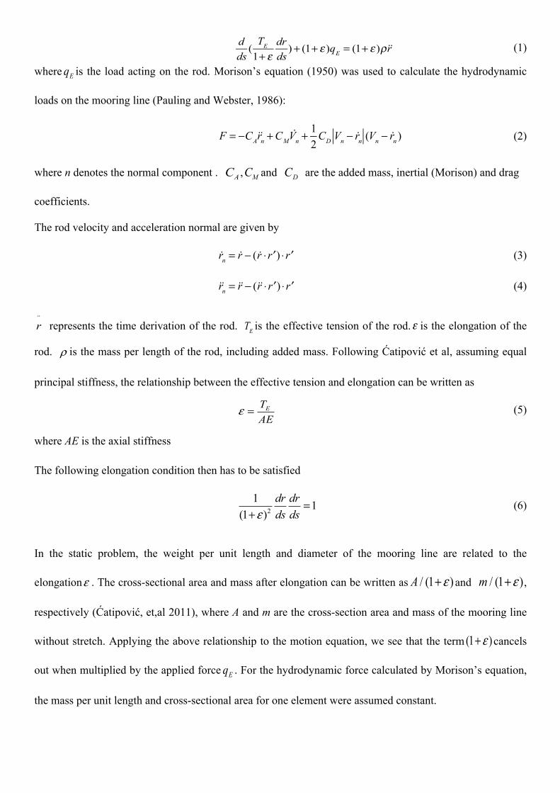
)+ (1+ ε )qE = (1+ ε )ρ!!r (1)

where Eq is the load acting on the rod. Morison’s equation (1950) was used to calculate the hydrodynamic

loads on the mooring line (Pauling and Webster, 1986):

F = −CA!!rn +CM

!Vn +12

CD Vn − !rn (Vn − !rn ) (2)

where n denotes the normal component . AC , MC and DC are the added mass, inertial (Morison) and drag

coefficients.

The rod velocity and acceleration normal are given by

!rn = !r − ( !r ⋅ ′r ) ⋅ ′r (3)

!!rn = !!r − (!!r ⋅ ′r ) ⋅ ′r (4)

r⋅⋅

represents the time derivation of the rod. TE is the effective tension of the rod.ε is the elongation of the

rod. ρ is the mass per length of the rod, including added mass. Following Ćatipović et al, assuming equal

principal stiffness, the relationship between the effective tension and elongation can be written as

ETAE

ε = (5)

where AE is the axial stiffness

The following elongation condition then has to be satisfied

2

1 1(1 )

dr drds dsε

=+

(6)

In the static problem, the weight per unit length and diameter of the mooring line are related to the

elongationε . The cross-sectional area and mass after elongation can be written as / (1 )A ε+ and / (1 )m ε+ ,

respectively (Ćatipović, et,al 2011), where A and m are the cross-section area and mass of the mooring line

without stretch. Applying the above relationship to the motion equation, we see that the term (1 )ε+ cancels

out when multiplied by the applied force Eq . For the hydrodynamic force calculated by Morison’s equation,

the mass per unit length and cross-sectional area for one element were assumed constant.

Equations (1) and (6) show the rod motion equation and elongation condition, respectively: they are

non-linear. In the following section, we will describe a numerical procedure for solving this non-linear

equation and the required order of approximation for the elongation condition.

2.2 Numerical Implementation

2.2.1 Static problem

For the static problem, r is independent of time. Consequently the inertial term in equation (1) is deleted.

We therefore have

( ) 01

EE

Td dr qds dsε

+ =+

(7)

Using the Taylor series expansion, the elongation relationship can be written as:

1(1+ε)2

=1− 2ε +3ε 2 +o(ε3) (8)

However, it is not clear, a priori, whether the third-order term should be included explicitly. In the present

paper, the order of expansion and subsequent results will be discussed.

In the FEM, the variables ri and TE may be approximated (Garrett, 1982) as

4

1( , ) ( ) ( )i k ik

kr s t A s U t

=

=∑ (9)

3

1( , ) ( ) ( )E m m

mT s t P s tλ

=

=∑ (10)

where Ak and Pm are shape functions. The definition of the shape functions can be found in the appendix.

Uik and λm are unknown variables. The subscript i of Uik denotes the dimension of the element. For the

3-dimensional problem, i=3. For k=1 and 3, Uik represents the space position of the rod at two ends while

Uik denotes the space derivative at both ends for k=2 and 4. λ is the Lagrange multiplier. The physical

meaning ofλ is mooring line tension at both ends and middle of the rod.

The variableUik and mλ are defined as:

1 2

3 4

(0, ), '(0, )( , ), '( , )

i i i i

i i i i

U r t U Lr tU r L t U Lr L t

= == =

(11)

1 2 3(0, ), ( , ), ( , )2Lt t L tλ λ λ λ λ λ= = = (12)

Using Galerkin’s method (Bathe, 1996) and integrating the motion equation from 0 to L over the length of

the element, the final form of motion equation for static problem in notation form can be written as

ˆ 0nijlk n jk ilK U Fλ − = (13)

where

0 1 2ˆnijlk nmijlk nmpijlkmnijlk m pK K K Kλ λλ= + + (14)

00

Lnijlk n l k ijP A A dsK δ′ ′= ∫ (15)

10

1Lnmijlk n m l k ijP P A A dsK EA

δ′ ′= −∫ (16)

220

1( )

Lnmqijlk n m q l k ijP P P A A dsK EA

δ′ ′= ∫ (17)

where δ is the Kronecker Delta function, L is the element length, and the standard double-suffix summation

condition has been used.

The elongation condition, incorporating Taylor series expansion to second order, can be written as

ˆ 0mil ki kl mB U U C− = (18)

where

0 1 2ˆmil nmil npmilmil n n pB B B Bλ λ λ= + + (19)

00

Lmil m i lP A AdsB ′ ′= ∫ (20)

10

2Lnmil m n i lP P A AdsB EA

′ ′= −∫ (21)

220

3( )

Lmnqil m n q i lP P P A AdsB EA

′ ′= ∫ (22)

0

L

m mC P ds= ∫ (23)

Recalling equation (13) and the elongation condition (18), Newton-Raphson iteration was applied to the

static problem (Ran, 2000). Omitting higher order components, we have

( 1) ( ) ( ) ( ) 0il iln njk nil il

njk

R RUR R U λλ

+ ∂ ∂= + Δ + Δ =∂ ∂

(24)

m(n+1)G = m

(n)G +∂ mG∂ jkU

(Δ jkU )+ ∂ mG∂ nλ

(Δ nλ ) = 0 (25)

Re-arranging the terms and writing in the matrix form, we have

11( ) 12( ) ( )ln

21( ) 22( ) ( )

n n njkijlk i il

n n nmn nmjk m

UK K RK K Gλ⎡ ⎤ Δ ⎧ ⎫⎧ ⎫

= −⎨ ⎬ ⎨ ⎬⎢ ⎥ Δ⎩ ⎭ ⎩ ⎭⎣ ⎦ (26)

where

( )11( ) ( )ˆ nn nnijlk nijlkK K λ= (27)

( )12( ) ( )ˆ nn niln jknijlkUK K= (28)

21( ) 12( )ln

n nmjk iK K= (29)

1 ( ) ( )22( ) 22 )( n nnmn pmnklp jl jkmnklB U UK Bλ= + (30)

( )( ) ( )ˆ nn nilil jknijlkUR FK= − (31)

( ) ˆnm mil ki kl mB U U CG = − (32)

The above formulation of the Newton-Raphson method can be written in matrix form

(n)K (Δy) = (n)F (33)

where K and F are the same as the stiffness matrix and forcing vector in equation (26). yΔ includes jkUΔ

and nλΔ . In the static problem, n represents the step of iteration.

2.2.2 Dynamic problem

The inertial term in the equation of motion equation cannot be neglected in the dynamic problem.

2 31 1 ( )(1 )

oε ε εε

= − + ++

(34)

The definition of ri and TE are the same as in the static case. Integrating over the element generates the

discretized form of the equation of motion. Incorporating the elongation condition, we have

ˆ ˆ( ) jkijlk jk n nijlk ilM U K FUλ= − + (35)

ˆ 0m mil ki kl m mt tG B U U B C λ= − − = (36)

where

ˆ aijlkijlk ijlkM M M= + (37)

To solve the second-order differential equation of motion, Ran (2000) introduced a new variable V :

M̂ijlk!Vjk = −λn K̂nijlk jkU + Fil (38)

!U jk =Vjk (39)

To solve these two equations, we need to integrate from t(n) to t(n+1), using the first-order Adam-Moulton

method. Ran assumed a constant value ( 0.5)ˆ nijlkM+ during this time interval, leading to the equation:

( ) ( )( 1) ( )

( ) 1( )

0 2 2 2 2

ˆ2 2 ( ) ( )

n nn n m m

m m jk njk n

n t nm nijlk il jk mn n

G GG G UU

G K U U D

λλ

λ

+ ∂ ∂= ≈ + Δ + Δ∂ ∂

= + Δ + Δ

(40)

Re-writing equations (38) and (40) in matrix form, we have

'11( ) '12( ) '( )ln

'21( ) '22( ) '( )

n n njkijlk i il

n n nmn nmjk m

UK K RK K Gλ⎡ ⎤ Δ ⎧ ⎫⎧ ⎫

= −⎨ ⎬ ⎨ ⎬⎢ ⎥ Δ⎩ ⎭ ⎩ ⎭⎣ ⎦ (41)

where

( 0.5) ( 0.5)'11( )

2

2 ˆˆ n nnijlk n nijlkijlk KK Mt

λ+ −= +Δ

(42)

'12( )ln

ˆ2ni nijlk jkK UK = (43)

'21( ) ˆ2nmjk mijlk ilK UK = (44)

'22( ) 22( )2( )n nmn mn mnCK K= + (45)

^( 0.5) ( ) ( ) ( ) ( 1)'( ) ( 0.5)2 ˆ 2 3n n n n nn n

nijlknil jk jk il ilijlk V K U F FR Mt λ+ −−= − + −Δ

(46)

m'(n)G = 2( m

(n)G −Cm ) (47)

The dynamic problem can be solved in a manner similar to the static case:

(n)K (Δy) = (n)F (48)

Now, n denotes the time step (instead of the iteration step in the static analysis). The static model was first

used to determine the mean position of the mooring line. The above numerical procedure was incorporated

in FAST’s FEM. The original FAST program, based on the assumption of small elongations was extended

to allow for large elongations, and therefore suitable for polyester lines. An advantage of the present method

is that the element stiffness matrix remains symmetric.

2.3 Validation of the enhanced model

The present study considered a model of a spar-type floating platform, similar to that used for a wind turbine

design of the National Renewable Energy Laboratory (NREL). The platform can be moored by slack or taut

mooring lines (ABS, 2014). In this paper, three equal taut mooring lines were selected for case studies. The

parameters of the floating cylinder and the upper structure are the same as NREL’s OC-3 Hywind Spar

(Jonkman, 2010), except for the mooring system. The main properties of the wind turbine are shown in

Table 1; those of the taut mooring line in Table 2. For simplicity, the Radius to Fairleads from Platform

Centreline in Table1 was 4.7m, instead of 5.2 m.

Figures 1 and 2 show the dynamic response of line tension in sea state 6 (H=5.5m, T=11.3s). The red line

shows the results of Fastlink (FAST+OrcaFlex). In Fastlink, OrcaFlex solves the dynamic response of

mooring line in the time domain and passes the mooring line tension to FAST for the coupled response of

the mooring system. From this comparison we can see that the Taylor expansion to second order (present)

shows little difference compared with the results from third order (extended stiffness). They both show very

good agreement with the lumped mass and spring method. However, when assuming small elongation

(equivalent to an expansion to first order, using the governing equation and elongation condition of the rod

by Pauling & Webster,1986) the blue and green lines in Figures 1 and 2 show poor results for a polyester

line.

The present enhanced stiffness method is also appropriate for a slack mooring line (catenary chain, line

length: 902.2m; chain mass: 77.7kg/m and elastic stiffness: 384.2E6 N). Figure 3 compares the line tension

results under sea state 6 for a catenary chain. Results from the approximation to second (reduced stiffness)

and third order (enhanced stiffness) generate the same results as OrcaFlex and the small elongation

assumption. From a comparison of Figures 1, 2 and 3 we can see that the present method can be used for

modelling both traditional materials as well as high-performance fibre. For the enhanced stiffness condition

(expansion to third order), the stiffness term and elongation are:

0 1 2 3ˆnijlk nmijlk nmpijlk nmpqijlkmnijlk m p q m pK K K K Kλ λ λ λ λλ= + + + (49)

0 1 2 3ˆmil nmil npmil npqmilmil n n p n p qB B B B Bλ λ λ λ λ λ= + + + (50)

330

1( )

Lnmtpqijlk n m q t l k ijP P P PA A dsK EA

δ′ ′= −∫ (51)

For the static problem,

330

4( )

Lnmqtil n m q t i lP P P PA A dsB EA

′ ′= −∫ (52)

while for the dynamic problem,

330

1( )

Lnpqmil n m q t i lP P P PA A dsB EA

′ ′= −∫ (53)

2.4 Comparison of line tension for different approximations

In order to check further the effect of differing elongation approximations, a reduced line length (420m) was

considered. Waves only were assumed, having the same height and frequency as above (sea state 6). The

elongation of the mooring line is about 15%, but the difference between values of the mean and maximum

line tension is around 1.3 % (see Figure 4, the mooring line layout is shown in Figure 5). So, the

approximation to second order is sufficient.

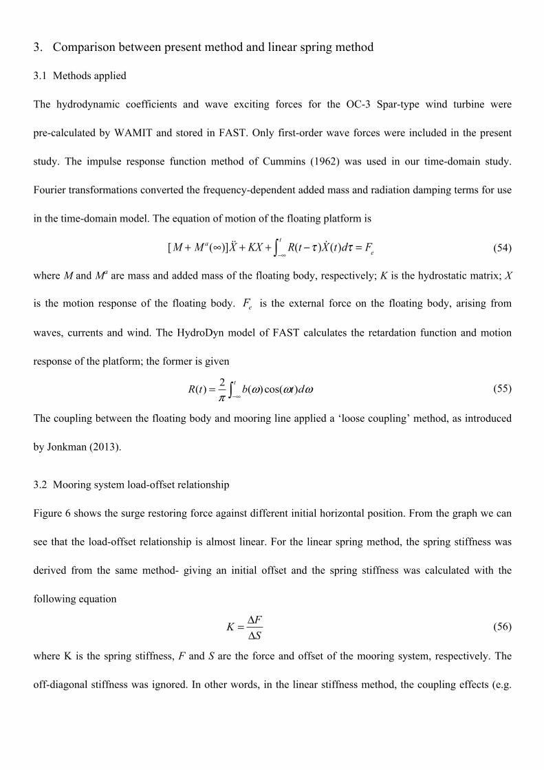
3. Comparison between present method and linear spring method

3.1 Methods applied

The hydrodynamic coefficients and wave exciting forces for the OC-3 Spar-type wind turbine were

pre-calculated by WAMIT and stored in FAST. Only first-order wave forces were included in the present

study. The impulse response function method of Cummins (1962) was used in our time-domain study.

Fourier transformations converted the frequency-dependent added mass and radiation damping terms for use

in the time-domain model. The equation of motion of the floating platform is

[M + M a (∞)] !!X + KX + R(t −τ )

−∞

t

∫ !X (t)dτ = Fe (54)

where M and Ma are mass and added mass of the floating body, respectively; K is the hydrostatic matrix; X

is the motion response of the floating body. eF is the external force on the floating body, arising from

waves, currents and wind. The HydroDyn model of FAST calculates the retardation function and motion

response of the platform; the former is given

2( ) ( )cos( )t

R t b t dω ω ωπ −∞

= ∫ (55)

The coupling between the floating body and mooring line applied a ‘loose coupling’ method, as introduced

by Jonkman (2013).

3.2 Mooring system load-offset relationship

Figure 6 shows the surge restoring force against different initial horizontal position. From the graph we can

see that the load-offset relationship is almost linear. For the linear spring method, the spring stiffness was

derived from the same method- giving an initial offset and the spring stiffness was calculated with the

following equation

FKS

Δ=Δ

(56)

where K is the spring stiffness, F and S are the force and offset of the mooring system, respectively. The

off-diagonal stiffness was ignored. In other words, in the linear stiffness method, the coupling effects (e.g.

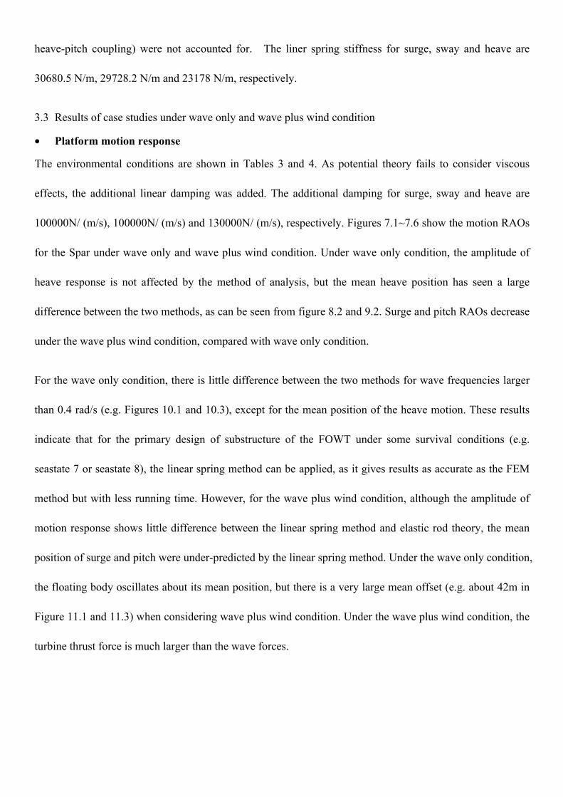
heave-pitch coupling) were not accounted for. The liner spring stiffness for surge, sway and heave are

30680.5 N/m, 29728.2 N/m and 23178 N/m, respectively.

3.3 Results of case studies under wave only and wave plus wind condition

• Platform motion response

The environmental conditions are shown in Tables 3 and 4. As potential theory fails to consider viscous

effects, the additional linear damping was added. The additional damping for surge, sway and heave are

100000N/ (m/s), 100000N/ (m/s) and 130000N/ (m/s), respectively. Figures 7.1~7.6 show the motion RAOs

for the Spar under wave only and wave plus wind condition. Under wave only condition, the amplitude of

heave response is not affected by the method of analysis, but the mean heave position has seen a large

difference between the two methods, as can be seen from figure 8.2 and 9.2. Surge and pitch RAOs decrease

under the wave plus wind condition, compared with wave only condition.

For the wave only condition, there is little difference between the two methods for wave frequencies larger

than 0.4 rad/s (e.g. Figures 10.1 and 10.3), except for the mean position of the heave motion. These results

indicate that for the primary design of substructure of the FOWT under some survival conditions (e.g.

seastate 7 or seastate 8), the linear spring method can be applied, as it gives results as accurate as the FEM

method but with less running time. However, for the wave plus wind condition, although the amplitude of

motion response shows little difference between the linear spring method and elastic rod theory, the mean

position of surge and pitch were under-predicted by the linear spring method. Under the wave only condition,

the floating body oscillates about its mean position, but there is a very large mean offset (e.g. about 42m in

Figure 11.1 and 11.3) when considering wave plus wind condition. Under the wave plus wind condition, the

turbine thrust force is much larger than the wave forces.

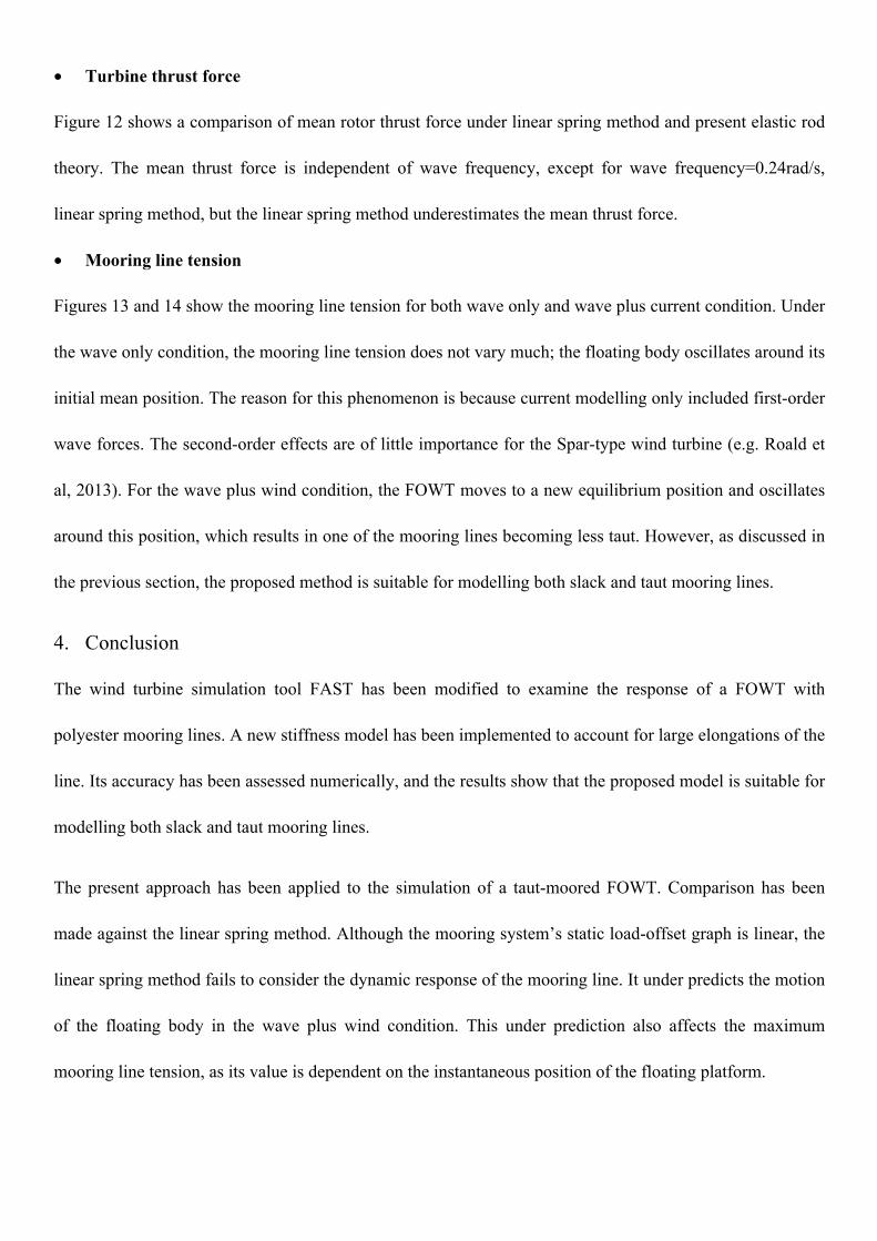
• Turbine thrust force

Figure 12 shows a comparison of mean rotor thrust force under linear spring method and present elastic rod

theory. The mean thrust force is independent of wave frequency, except for wave frequency=0.24rad/s,

linear spring method, but the linear spring method underestimates the mean thrust force.

• Mooring line tension

Figures 13 and 14 show the mooring line tension for both wave only and wave plus current condition. Under

the wave only condition, the mooring line tension does not vary much; the floating body oscillates around its

initial mean position. The reason for this phenomenon is because current modelling only included first-order

wave forces. The second-order effects are of little importance for the Spar-type wind turbine (e.g. Roald et

al, 2013). For the wave plus wind condition, the FOWT moves to a new equilibrium position and oscillates

around this position, which results in one of the mooring lines becoming less taut. However, as discussed in

the previous section, the proposed method is suitable for modelling both slack and taut mooring lines.

4. Conclusion

The wind turbine simulation tool FAST has been modified to examine the response of a FOWT with

polyester mooring lines. A new stiffness model has been implemented to account for large elongations of the

line. Its accuracy has been assessed numerically, and the results show that the proposed model is suitable for

modelling both slack and taut mooring lines.

The present approach has been applied to the simulation of a taut-moored FOWT. Comparison has been

made against the linear spring method. Although the mooring system’s static load-offset graph is linear, the

linear spring method fails to consider the dynamic response of the mooring line. It under predicts the motion

of the floating body in the wave plus wind condition. This under prediction also affects the maximum

mooring line tension, as its value is dependent on the instantaneous position of the floating platform.

ACKNOWLEDGMENT

The authors gratefully acknowledge the assistance of Dr. Jason Jonkman in his responses to questions about

the simulation tool FAST. This research was supported by the Department of Naval Architecture, Ocean and

Marine Engineering and the Faculty of Engineering at the University of Strathclyde and by the China

Scholarship Council (CSC).

REFERENCE

1. ABS, 2014. Global performance analysis for floating offshore wind turbine installations.

2. Agarwal, A.K., Jain, A.K., 2003. Dynamic behaviour of offshore spar platforms under regular sea waves

Ocean Engineering, 30 (4), pp. 487-516.

3. Bathe K. J., 1996. Finite element procedures, Prentice Hall, chapter 6.

4. Ćatipović, I., Čorić, V. and Radanović, J., 2011. An improved stiffness model for polyester mooring lines.

Brodogradnja, 62(3), pp. 235-248.

5. Chen X. H., 2002. Studies on dynamic iteration between deep-water floating structure and their

mooring/tendon systems. Dissertation, Texas A&M University.

6. Cummins W.E., 1962, the impulse response function and ship motions, DTMB Report 1661, Washington

D.C.

7. Deep Water- The next step for offshore wind energy, a report by the EWEA, July 2013.

8. Garrett, D.L., 1982. Dynamic analysis of slender rods. J Energy Resour Technol Trans Asme, v 104(n 4),

pp. 302-306.

9. Goupee, A.J., Koo, B.J., Kimball, R.W., Lambrakos, K.F., Dagher, H.J., 2014. Experimental comparison

of three floating wind turbine concepts. Journal of Offshore Mechanics and Arctic Engineering, 136 (2).

10. Jonkman, J., 2010. Definition of the floating System for phase IV of OC3. NREL/TP-500-47535,

Golden, CO: National Renewable Energy Laboratory.

11. Jonkman, J.M., 2013. The new modularization framework for the FAST wind turbine CAE tool, 51st

AIAA Aerospace Sciences Meeting including the New Horizons Forum and Aerospace Exposition.

12. Kim, B.W., Sung, H.G., Kim, J.H. and Hong, S.Y., 2013. Comparison of linear spring and nonlinear

FEM methods in dynamic coupled analysis of floating structure and mooring system. Journal of Fluids and

Structures, 42, pp. 205-227.

13. Kim, C.H., Kim, M.H., Liu, Y.H. and Zhao, C.T., 1994. Time domain simulation of nonlinear response

of a coupled TLP system. International Journal of Offshore and Polar Engineering, 4(4), pp. 284-291.

14. Kim, J.W., Sablok, A., Kyoung, J.H. and Lambrakos, K., 2011. A nonlinear viscoelastic model for

polyester mooring line analysis, Proceedings of the International Conference on Offshore Mechanics and

Arctic Engineering - OMAE 2011, pp. 797-803.

15. Kim, M.H., Arcandra and Kim, Y.B., 2001. Variability of spar motion analysis against design

methodologies/parameters, Proceedings of the International Conference on Offshore Mechanics and Arctic

Engineering - OMAE 2001, pp. 153-161.

16. Kreuzer, E. and Wilke, U., 2003. Dynamics of mooring systems in ocean engineering. Archive of

Applied Mechanics, 73(3-4), pp. 270-281.

17. Love A., 1944.Treatise on the mathematical theory of elasticity. Over Publications New York.

18. Low Y. M., 2006. Efficient methods for the dynamic analysis of deepwater offshore production systems,

PhD Thesis, University of Cambridge.

19. Morison J. R., O'Brien M. R., Johnson J. W., Schaaf S.,1950. A., The forces exerted by surface waves

on piles. Petroleum Transactions, AIME189:149–154.

20. NWTC Computer-Aided Engineering Tools (FAST by Jason Jonkman, Ph.D.).

http://wind.nrel.gov/designcodes/simulators/fast/. Last modified 2-July-2014; accessed 1-September-2014.

21. Nordgren, R.P., On computation of the motion of elastic rods,1974. Journal of Applied Mechanics,

Transactions of the ASME, 41 Ser E (2), pp. 777-780.

22. OrcaFlex user manual Version 9.7a. Orcina Ltd. Daltongate, Ulverston Cumbria. LA12 7AJ, UK

23. Pauling J. R., Webster W.C., 1986. A consistent large amplitude analysis of the coupled response of a

TLP and tendon system. Proceedings of the International Conference on Offshore Mechanics and Arctic

Engineering -OMAE 1986 Vol 3, p 126

24. Ran Z.,2000. Coupled dynamic analysis of floating structures in waves and currents. Dissertation, Texas

A&M University.

25. Arcandra, Tahar,2001. Hull/mooring/riser coupled dynamic analysis of a floating platform with

polyester mooring lines. Dissertation, Texas A&M University.

26. Roald, L., Jonkman, J., Robertson, A. and Chokani, N., 2013. The effect of second-order

hydrodynamics on floating offshore wind turbines, Energy Procedia 2013, pp. 253-264.

Appendix

SHAPE FUNCTIONS

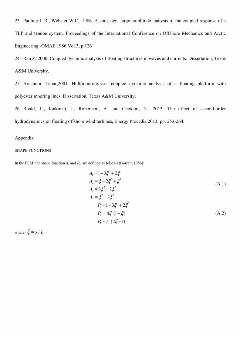
In the FEM, the shape function Al and Pm are defined as follows (Garrett, 1986):

2 31

2 32

2 33

2 34

1 3 2

2

3 2

2

A

A

A

A

ξ ξξ ξ ξξ ξξ ξ

= − +

= − +

= −

= −

(A.1)

21

2

3

1 3 2

4 (1 )

(2 1)

P

P

P

ξ ξξξ

ξξ

= − +

= −

= −

(A.2)

where /s Lξ =