an empirical comparison of machine learning models for time series forecasting

PLEASE SCROLL DOWN FOR ARTICLE

This article was downloaded by: [Atiya, Amir]On: 15 September 2010Access details: Access Details: [subscription number 926965465]Publisher Taylor & FrancisInforma Ltd Registered in England and Wales Registered Number: 1072954 Registered office: Mortimer House, 37-41 Mortimer Street, London W1T 3JH, UK

Econometric ReviewsPublication details, including instructions for authors and subscription information:http://www.informaworld.com/smpp/title~content=t713597248

An Empirical Comparison of Machine Learning Models for Time SeriesForecastingNesreen K. Ahmeda; Amir F. Atiyab; Neamat El Gayarc; Hisham El-Shishinyd

a Department of Computer Science, Purdue University, West Lafayette, Indiana, USA b Department ofComputer Engineering, Cairo University, Giza, Egypt c Faculty of Computers and Information, CairoUniversity, Giza, Egypt d IBM Center for Advanced Studies in Cairo, IBM Cairo TechnologyDevelopment Center, Giza, Egypt

Online publication date: 15 September 2010

To cite this Article Ahmed, Nesreen K. , Atiya, Amir F. , Gayar, Neamat El and El-Shishiny, Hisham(2010) 'An EmpiricalComparison of Machine Learning Models for Time Series Forecasting', Econometric Reviews, 29: 5, 594 — 621To link to this Article: DOI: 10.1080/07474938.2010.481556URL: http://dx.doi.org/10.1080/07474938.2010.481556

Full terms and conditions of use: http://www.informaworld.com/terms-and-conditions-of-access.pdf

This article may be used for research, teaching and private study purposes. Any substantial orsystematic reproduction, re-distribution, re-selling, loan or sub-licensing, systematic supply ordistribution in any form to anyone is expressly forbidden.

The publisher does not give any warranty express or implied or make any representation that the contentswill be complete or accurate or up to date. The accuracy of any instructions, formulae and drug dosesshould be independently verified with primary sources. The publisher shall not be liable for any loss,actions, claims, proceedings, demand or costs or damages whatsoever or howsoever caused arising directlyor indirectly in connection with or arising out of the use of this material.

http://www.informaworld.com/smpp/title~content=t713597248

http://dx.doi.org/10.1080/07474938.2010.481556

http://www.informaworld.com/terms-and-conditions-of-access.pdf

Econometric Reviews, 29(5–6):594–621, 2010Copyright © Taylor & Francis Group, LLCISSN: 0747-4938 print/1532-4168 onlineDOI: 10.1080/07474938.2010.481556

AN EMPIRICAL COMPARISON OF MACHINE LEARNINGMODELS FOR TIME SERIES FORECASTING

Nesreen K. Ahmed1, Amir F. Atiya2, Neamat El Gayar3,and Hisham El-Shishiny4

1Department of Computer Science, Purdue University, West Lafayette, Indiana, USA2Department of Computer Engineering, Cairo University, Giza, Egypt3Faculty of Computers and Information, Cairo University, Giza, Egypt4IBM Center for Advanced Studies in Cairo, IBM Cairo TechnologyDevelopment Center, Giza, Egypt

� In this work we present a large scale comparison study for the major machine learningmodels for time series forecasting. Specifically, we apply the models on the monthly M3 timeseries competition data (around a thousand time series). There have been very few, if any,large scale comparison studies for machine learning models for the regression or the time seriesforecasting problems, so we hope this study would fill this gap. The models considered aremultilayer perceptron, Bayesian neural networks, radial basis functions, generalized regressionneural networks (also called kernel regression), K-nearest neighbor regression, CART regressiontrees, support vector regression, and Gaussian processes. The study reveals significant differencesbetween the different methods. The best two methods turned out to be the multilayer perceptronand the Gaussian process regression. In addition to model comparisons, we have tested differentpreprocessing methods and have shown that they have different impacts on the performance.

Keywords Comparison study; Gaussian process regression; Machine learning models; Neuralnetwork forecasting; Support vector regression.

JEL Classification C45; C4.

1. INTRODUCTION

Machine learning models have established themselves in the lastdecade as serious contenders to classical statistical models in the areaof forecasting. Research started in the eighties with the development of

Address correspondence to Amir F. Atiya, Department of Computer Engineering, CairoUniversity, Giza, Egypt; E-mail: [email protected]

Downloaded By: [Atiya, Amir] At: 11:27 15 September 2010

An Empirical Comparison 595

the neural network model. Subsequently, research extended the conceptto other models, such as support vector machines, decision trees, andothers, that are collectively called machine learning models (Alpaydin,2004; Hastie et al., 2001). Some of these models trace their origins fromthe early statistics literature (see Hastie et al., 2001 for a discussion). Therehave been impressive advances in this field in the past few years, bothin the theoretical understanding of the models and in the amount andvariations of the models developed. In addition to model developmentand analysis there has to be a parallel effort of empirically validating thenumerous existing models and comparing their performance. This wouldbe of immense value to the practitioner, as it would narrow down hispossible choices, and give him insight into the strong and weak pointsof the available models. In addition, this would also help to channel theresearch effort into the more promising tracks.

Large scale studies for comparing machine learning models havefocused almost exclusively on the classification domain (Caruana andNiculescu-Mizil, 2006). We have found no extensive study for regressionproblems. There have been numerous comparison studies that compareneural networks with traditional linear techniques for forecasting andother econometric problems. For example, Sharda and Patil (1992) havecompared neural networks to ARIMA on the M-competition time seriesdata. Hill et al. (1996) have also considered the M-competition dataand have compared between neural networks and traditional methods.Swanson and White (1995) have applied their comparison on nine U.S.macroeconomic series. Alon et al. (2001) have analyzed neural networksversus other traditional methods such as Winters exponential smoothing,Box–Jenkins ARIMA and multivariate regression, on retail sales data.Callen et al. (1996) have compared between neural networks and linearmodels for 296 quarterly earnings time series. Zhang et al. (2004) haveconsidered a similar problem, but have added some additional accountingvariables. Terasvirta et al. (2005) consider neural networks, smoothtransition autoregressions, and linear models for 47 macroeconomic series.The outcome of all these studies has been somewhat mixed, but overallneural networks tended more to outperform classical linear techniques.

The problem is that these studies are confined to only the basicneural network model, and do not extend to the novel machine learningmodels. This, in fact, is the subject of this study. We conduct a large scalecomparison study of a variety of machine learning models applied to theM3 competition data (M3 Competition, 2008). The M3 competition is thelatest in a sequel of M forecasting competitions, organized by Makridakisand Hibon (2000). It consists of 3003 business-type time series, coveringthe types of micro, industry, finance, demographic, and others. There areyearly, quarterly, and monthly time series. In this study, we consider onlythe monthly time series, as quarterly and yearly time series were generally


596 N. K. Ahmed et al.

too short. The M3 data has become an important benchmark for testingand comparing forecasting models. Having that many diverse time seriesgives confidence into comparison results. The training period for theconsidered time series ranges in length from 63 to 108 data points, so thecomparison study will generally apply to the kinds of monthly business timeseries of this length range.

In this study, we have compared the following models: multilayerperceptron, Bayesian neural networks, radial basis functions, generalizedregression neural networks (also called kernel regression), K-nearestneighbor regression, CART regression trees, support vector regression, andGaussian processes. Another focus of the study is to examine preprocessingmethods, used in conjunction with the machine learning forecastingmodels. Preprocessing steps such as deseasonalization, taking the logtransformation, and detrending have been studied before in the literature(Balkin and Ord, 2000; Ghysels et al., 1996; Miller and Williams, 2004;Zhang and Qi, 2005; Zhang et al., 2004). These methods will, therefore,not be the focus of the comparison study. The goal in this study isto compare other preprocessing strategies that are frequently used withmachine learning models, such as differencing the time series, and takingmoving averages.

To summarize the findings of the paper the overall ranking of themodels from best to worse turned out to be about: multilayer perceptron,Gaussian processes, then Bayesian neural networks and support vectorregression almost similar, then generalized regression neural networks andK-nearest neighbor regression about tied, CART regression trees, then inthe last spot radial basis functions. This ranking is generally broad-basedand does not change much with different categories or features of thetime series. The preprocessing method can also have a large impact onperformance.

The article is organized as follows. Next section we present a briefdescription of the compared models. Section 3 describes the testedpreprocessing methods. Section 4 deals with the issue of how to set themodel parameters. In Section 5 we describe the details of the simulationssetup. Following that, in Section 6 we present the comparison results.Section 7 gives some comments on the results, and finally Section 8presents the conclusion of the article.

2. MODELS

For each considered model there are myriads of variations proposedin the literature, and it would be a hopeless task to consider all existingvarieties. Our strategy was therefore to consider the basic version ofeach model (without the additions, or the modifications proposed by somany researchers). The rationale is that most users will more likely opt



(at least in their first try) to consider the basic form. For example forthe K-nearest neighbor model (KNN), we used the basic form where thetarget outputs of the K-neighbors are equally weighted. There are manyother variations, such as distance weighted KNN, flexible metric KNN,non-Euclidean distance-based, and so on, but we did not consider thesevariants.

The reason for generally selecting these considered eight models isthat they are some of the most commonly used models. Below is a shortdescription of the models considered.

2.1. Multilayer Perceptron (MLP)

The multilayer perceptron (often simply called neural network) isperhaps the most popular network architecture in use today both forclassification and regression (Bishop, 1995). The MLP is given as follows:

y = v0 +NH∑j=1

vjg(wT

j x′), (1)

where x ′ is the input vector x , augmented with 1, i.e., x ′ = (1, xT )T , wj isthe weight vector for j th hidden node, v0, v1, � � � , vNH are the weights forthe output node, and y is the network output. The function g representsthe hidden node output, and it is given in terms of a squashing function,for example (and that is what we used) the logistic function: g (u) = 1/(1 +exp(−u)). A related model in the econometrics literature is the smoothtransition autoregression model that is also based on constructing linearfunctions and logistic function transitions (Medeiros and Veiga, 2000; vanDijk et al., 2002).

The MLP is a heavily parametrized model, and by selecting the numberof hidden nodes NH we can control the complexity of the model. Thebreakthrough that lent credence to the capability of neural networks isthe universal approximation property (Cybenko, 1989; Funahashi, 1989;Hornik et al., 1989; Leshno et al., 1993). Under certain mild conditions onthe hidden node functions g , any given continuous function on a compactset can be approximated as close as arbitrarily given using a network witha finite number of hidden nodes. While this is a reassuring result, it iscritical to avoid overparametrization, especially in forecasting applicationswhich typically have a limited amount of highly noisy data. Model selection(via selecting the number of hidden nodes) has therefore attracted muchinterest in the neural networks literature (see Anders and Korn, 1999;Medeiros et al., 2006 for example). We use a K-fold validation procedureto select the number of hidden nodes, but the details of this (and anyparameter selection step) will be discussed in the next section.



To obtain the weights, the mean square error is defined, andthe weights are optimized using gradient techniques. The most well-known method, based on the steepest descent concept, is the back-propagation algorithm. A second order optimization method calledLevenberg Marquardt is generally known to be more efficient than thebasic back-propagation algorithm, and this is the one we used in ourimplementation (we use the Matlab function trainlm).

2.2. Bayesian Neural Network (BNN)

A Bayesian neural network (BNN) is a neural network designedbased on a Bayesian probabilistic formulation (MacKay, 1992a,b). As suchBNN’s are related to the classical statistics concept of Bayesian parameterestimation, and are also related to the concept of regularization such as inridge regression. BNN’s have enjoyed wide applicability in many areas suchas economics/finance (Gencay and Qi, 2001) and engineering (Bishop,1995). The idea of BNN is to treat the network parameters or weightsas random variables, obeying some a priori distribution. This distributionis designed so as to favor low complexity models, i.e., models producingsmooth fits. Once the data are observed, the posterior distribution of theweights is evaluated and the network prediction can be computed. Thepredictions will then reflect both the smoothness aspect imposed throughthe prior and the fitness accuracy aspect imposed by the observed data.A closely related concept is the regularization aspect, whereby the followingobjective function is constructed and minimized

J = �ED + (1 − �)EW , (2)

where ED is the sum of the square errors in the network outputs, EW is thesum of the squares of the network parameters (i.e., weights), and � is theregularization parameter.

For the Bayesian approach, the typical choice of the prior is thefollowing normal density that puts more weight onto smaller networkparameter values

p(w) =(1 − �

�

) L2

e−(1−�)EW , (3)

where L denotes the number of parameters (weights). The posterior isthen given by

p(w |D, �) = p(D |w, �)p(w | �)p(D | �) , (4)



where D represents the observed data. Assuming normaly distributederrors, the probability density of the data given the parameters can beevaluated as

p(D |w, �) =(�

�

)M2

e−�ED , (5)

where M is the number of training data points. By substituting theexpressions for the densities in (3) and (5) into (4), we get

p(w |D, �) = c exp(−J ), (6)

where c is some normalizing constant. The regularization constant � is alsodetermined using Bayesian concepts, from

p(� |D) = p(D | �)p(�)p(D)

� (7)

Both expressions (6) and (7) should be maximized to obtain the optimalweights and � parameter, respectively. The term p(D | �) in (7) is obtainedby a quadratic approximation of J in terms of the weights and thenintegrating out the weights. We used the Matlab version version ‘trainbr’for BNN (applied to a multilayer perceptron architecture). This routineis based on the algorithm proposed by Foresee and Hagan (1997). Thisalgorithm utilizes the Hessian that is obtained any way in the Levenberg–Marquardt optimization algorithm in approximating (7).

2.3. Radial Basis Function Neural Network (RBF)

The radial basis function network is similar in architecture to themultilayer network except that the nodes have a localized activationfunction (Moody and Darken, 1989; Powell, 1987). Most commonly, nodefunctions are chosen as Gaussian functions, with the width of the Gaussianfunction controlling the smoothness of the fitted function. The outputsof the nodes are combined linearly to give the final network output.Specifically, the output is given by

y =NB∑j=1

wj e− ‖x−cj ‖2

�2 , (8)

where wj , �, and cj denote respectively the combining weight, the width ofthe node function, and the center of the node function for unit j . Becauseof the localized nature of the node functions, other simpler algorithmshave been developed for training radial basis networks. The algorithm we



used is the Matlab function (newrb). It is based on starting with a blanknetwork, and sequentially adding nodes until an acceptable error in thetraining set is achieved. Specifically, we add a node centered around thetraining pattern giving the maximum error. Then we recompute all theoutput layer weights using the least squares formula. We continue thisway until the error limit is reached or the number of nodes reaches amaximum predetermined value. While there are a variety of other RBFtraining algorithms, we opted for this one due to its availability in theMatlab suite, and hence it will be more likely selected by the user interestedin RBF’s.

2.4. Generalized Regression Neural Network (GRNN)

Nadaraya and Watson developed this model (Nadaraya, 1964; Watson,1964). It is commonly called the Nadaraya–Watson estimator or thekernel regression estimator. In the machine learning community, the termgeneralized regression neural network (or GRNN) is typically used. Wewill use this latter term. The GRNN model is a nonparametric modelwhere the prediction for a given data point x is given by the average ofthe target outputs of the training data points in the vicinity of the givenpoint x (Hardle, 1990). The local average is constructed by weighting thepoints according to their distance from x , using some kernel function. Theestimation is just the weighted sum of the observed responses (or targetoutputs) given by

y =M∑

m=1

wmym , (9)

where the weights wm are given by

wm = �( ‖x−xm‖

h

)∑M

m ′=1 �( ‖x−xm′ ‖

h

) , (10)

where ym is the target output for training data point xm , and � is thekernel function. We used the typical Gaussian kernel �(u) = e−u2/2/

√2�.

The parameter h, called the bandwidth, is an important parameter as itdetermines the smoothness of the fit, since increasing it or decreasing itwill control the size of the smoothing region.

2.5. K Nearest Neighbor Regression (KNN)

The K nearest neighbor regression method (KNN) is a nonparametricmethod that bases its prediction on the target outputs of the K nearest



neighbors of the given query point (see Hastie et al., 2001). Specifically,given a data point, we compute the Euclidean distance between that pointand all points in the training set. We then pick the closest K training datapoints and set the prediction as the average of the target output values forthese K points. Quantitatively speaking, let �(x) be the set of K nearestneighbors of point x . Then the prediction is given by

y = 1K

∑m∈�(x)

ym , (11)

where again ym is target output for training data point xm .Naturally K is a key parameter in this method, and has to be selected

with care. A large K will lead to a smoother fit, and therefore a lowervariance, of course at the expense of a higher bias, and vice versa for asmall K .

2.6. Classification and Regression Trees (CART)

CART is a classification or regression model that is based on ahierarchical tree-like partition of the input space (Breiman, 1993).Specifically, the input space is divided into local regions identified in asequence of recursive splits. The tree consists of internal decision nodesand terminal leaves. Given a test data point, a sequence of tests along thedecision nodes starting from the root node will determine the path alongthe tree till reaching a leaf node. At the leaf node, a prediction is madeaccording to the local model associated with that node.

To construct a tree using the training set, we start at the root node. Weselect the variable (and its split threshold) whose splitting will lead to thelargest reduction in mean square error. We continue these splits recursively,until the mean square error reaches an acceptable threshold. A typicalpractice is to perform some kind of pruning for the tree, once designed.This will eliminate ineffective nodes and keep in check model complexity.To implement CART, we used the Matlab function (treefit).

2.7. Support Vector Regression (SVR)

Support vector regression (Scholkopf and Smola, 2001; Smola andScholkopf, 2003) is a successful method based on using a high-dimensionalfeature space (formed by transforming the original variables), andpenalizing the ensuing complexity using a penalty term added to the errorfunction. Consider first for illustration a linear model. Then, the predictionis given by

f (x) = wTx + b (12)



where w is the weight vector, b is the bias and x is the input vector. Letxm and ym denote, respectively, the mth training input vector and targetoutput, m = 1, � � � ,M . The error function is given by

J = 12‖w‖2 + C

M∑m=1

|ym − f (xm)|�� (13)

The first term in the error function is a term that penalizes modelcomplexity. The second term is the �-insensitive loss function, definedas |ym − f (xm)|� = max�0, |ym − f (xm)| − ��. It does not penalize errorsbelow �, allowing it some wiggle room for the parameters to move toreduce model complexity. It can be shown that the solution that minimizesthe error function is given by

f (x) =M∑

m=1

(�∗m − �m)xT

m x + b, (14)

where �m and �∗m are Lagrange multipliers. The training vectors giving

nonzero Lagrange multipliers are called support vectors, and this is a keyconcept in SVR theory. Non-support vectors do not contribute directly tothe solution, and the number of support vectors is some measure of modelcomplexity (see Chalimourda et al., 2004; Cherkassky and Ma, 2004). Thismodel is extended to the nonlinear case through the concept of kernel �,giving a solution

f (x) =M∑

m=1

(�∗m − �m)�(xT

m x) + b� (15)

A common kernel is the Gaussian kernel. Assume its width is �K (thestandard deviation of the Gaussian function). In our simulations, we usedthe toolbox by Canu at al. (2005).

2.8. Gaussian Processes (GP)

Gaussian process regression is a nonparametric method based onmodeling the observed responses of the different training data points(function values) as a multivariate normal random variable (see a detailedtreatise in Rasmussen and Williams, 2006). For these function values an apriori distribution is assumed that guarantees smoothness properties of thefunction. Specifically, the correlation between two function values is highif the corresponding input vectors are close (in Euclidean distance sense)and decays as they go farther from each other. The posterior distribution



of a to-be-predicted function value can then be obtained using the assumedprior distribution by applying simple probability manipulations.

Let V (X ,X ) denote the covariance matrix between the function values,where X is the matrix of input vectors of the training set (let the (i , j)thelement of V (X ,X ) be V (xi , xj), where xi denotes the ith training inputvector). A typical covariance matrix is the following:

V (xi , xj) = �2f e

− ‖xi−xj ‖222 � (16)

Thus, the vector of function values f (where fi is the function value fortraining data point i) obeys the following multivariate Gaussian density:

f ∼ �f (0,V (X ,X )), (17)

where �f (,�) denotes a multivariate normal density function in variablef with mean and covariance matrix �.

In addition, some independent zero-mean normally distributed noisehaving standard deviation �n is assumed to be added to the function valuesto produce the observed responses (target values), i.e.,

y = f + �, (18)

where y is the vector of target outputs and � is the vector of additive noise,whose components are assumed to be independent. The terms fi representthe inherent function values, and these are the values we would like topredict, particularly for the test data.

Then, for a given input vector x∗, the prediction f∗ is derived as

f∗ = E(f∗|X , y, x∗

) = V (x∗,X )[V (X ,X ) + �2

nI]−1

y� (19)

This equation is obtained by standard manipulations using Bayes ruleapplied on the given normal densities.

3. PREPROCESSING METHODS

Preprocessing the time series can have a big impact on the subsequentforecasting performance. It is as if we are “making it easier” for theforecasting model by transforming the time series based on informationwe have on some of its features. For example, a large number of empiricalstudies advocate the deseasonalization of data possessing seasonalitiesfor neural networks (Balkin and Ord, 2000; Miller and Williams, 2004;Zhang and Qi, 2005). Other preprocessing methods such as taking a logtransformation and detrending have also been studied in the literature.



We will use a deseasonalization step (if needed) and a log-step; however,these are not the object of this comparison study. What would be morenovel is to compare some of the other preprocessing typically used formachine learning forecasting models, as there are very few comparisonstudies (if any) that consider these. The methods considered are (let ztdenote the time series):

1. No special preprocessing (LAGGED-VAL): the input variables to themachine learning model are the lagged time series values (sayzt−N+1, � � � , zt), and the value to be predicted (target output) is the nextvalue (for one-step ahead forecasting);

2. Time series differencing (DIFF): We take the first backward differenceand apply the forecasting model on this differenced series;

3. Taking moving averages (MOV-AVG): We compute moving averages withdifferent-sized smoothing windows, for example,

ui(t) = 1Ji

t∑j=t−Ji+1

zj , i = 1, � � � , I , (20)

where Ji is the size of the averaging window (the Ji ’s in our case take thevalues 1, 2, 4, 8). The new input variables for the forecasting model wouldthen be ui(t) and the target output is still zt+1. The possible advantage ofthis preprocessing method is that moving averages smooth out the noise inthe series, allowing the forecasting model to focus on the global propertiesof the time series. The existence of several moving averages with differentsmoothing levels is important so as to preserve different levels of time seriesdetail in the set of inputs.

A note on the differencing issue (Point 2 above) is that whiledifferencing for linear models is a well-understood operation havingprincipled tests to determine its need, this is not the case for nonlinearmodels. The situation there is more ad hoc, as our experience and studieson other time series have demonstrated that differencing is not always agood strategy for nonstationary time series, and the converse is true forstationary time series. Here we attempt to shed some light on the utility ofdifferencing.

4. PARAMETER DETERMINATION

For every considered method there are typically a number ofparameters, some of them are key parameters and have to be determinedwith care. The key parameters are the ones that control the complexity ofthe model (or in short model selection parameters). These are the numberof input variables given to the machine learning model (for example the



number of lagged variables N for LAGGED-VAL and DIFF), the size of thenetwork (for MLP and for BNN), the width of the radial bases � for RBF,the number of neighbors K for KNN, the width of the kernels h for GRNN,and for each of SVR and GP we have three parameters (we will discuss themlater).

For linear models, the typical approach for model selection is to use aninformation criterion such as Akaike’s criterion, the Bayesian informationcriterion, or others, which consider a criterion consisting of the estimationerror added to it a term penalizing model complexity. For machinelearning approaches such criteria are not well-developed yet. Even thoughsome theoretical analyses have obtained some formulas relating expectedprediction error with the estimation error (training error) and modelcomplexity (Magdon-Ismail et al., 1998; Moody, 1992; Murata et al., 1993),these formulas are mostly bounds and have not been tested enough togain acceptance in practical applications. The dominant approach in themachine learning literature has been to use the K-fold validation approachfor model selection. Empirical comparisons indicate its superiority forperformance accuracy estimation and for model selection (Kohavi, 1995)over other procedures such as the hold out, the leave one out, and thebootstrap methods. In the K-fold validation approach the training set isdivided into K equal parts (or folds). We train our model using the datain the K − 1 folds and validate on the remaining K th fold. Then we rotatethe validation fold and repeat with the same procedure again. We performthis training and validation K times, and compute the sum of the validationerrors obtained in the K experiments. This will be the validation error thatwill be used as a criterion for selecting the key parameters (we used K = 10in our implementation, as this is generally the best choice according toKohavi, 1995).

For each method there are generally two parameters (or more) thathave to be determined using the K-fold validation: the number of inputvariables (i.e., the number of lagged variables N ), and the parameterdetermining the complexity (for example, the number of hidden nodesfor MLP, say NH ). We consider a suitable range for each parameter, sofor N we consider the possible values [1, 2, � � � , 5], and for NH we considerthe candidate values NH = [0, 1, 3, 5, 7, 9] (0 means a linear model). First,we fix NH as the median of the candidate NH values, and perform 10-fold validation to select N . Then we fix this selected N and perform a10-fold validation to select NH . Note that for MLP we have the possibilityof “having zero hidden nodes" (NH = 0), meaning simply a linear model.Balkin and Ord (2000) have shown that the possibility of switching toa linear model improved performance. We perform a similar tuningprocedure as above for all models (except GP as we will see later). Thefollowing are the ranges of the parameters of the other models. For BNN,the number of hidden nodes is selected from the candidate values NH =



[1, 3, 5, 7, 9]. Note that BNN does not encompass a linear model like MLP,because as developed in Foresee and Hagan (1997) and MacKay (1992b)it applies only to a multilayer network. For a linear model it has to berederived, leading to some form of a shrinkage-type linear model. ForRBF the width of the radial bases � is selected from the possible values[2�5, 5, 7�5, 10, 12�5, 15, 17�5, 20]. For GRNN the bandwidth parameter h isselected from [0�05, 0�1, 0�2, 0�3, 0�5, 0�6, 0�7]. The number of neighbors Kin the KNN model is tested from the possibilities [2, 4, 6, 8, 12, 16, 20].

For the case of SVM the key parameters that control the complexityof the model are �, C , and �K . In Cherkassky and Ma (2004) and inChalimourda et al. (2004) a comprehensive analysis of these parametersand their effects on the out-of-sample prediction performance and modelcomplexity is presented. Chalimourda et al. (2004) and Mattera and Haykin(1999) argue that C be set as the maximum of the target output valuesymax, and that the prediction performance should not be very sensitive tothe value of C . Using theoretical as well as experimental analysis Kwok(2001) suggests that � should be set equal to the noise level in thedata. Chalimourda et al. (2004) argue that the prediction performance issensitive to �K , and that this parameter has to be carefully selected. Wefollowed the lead and fixed C as ymax. We allowed � and �K to be set using10-fold validation. We consider a two-dimensional grid of � and �K using thevalues �y ∗ [0�5, 0�75, 1, 1�25, 1�5] × �0 ∗ [0�05, 0�1, 0�25, 0�5, 1, 2, 4]. The term�y is the estimated noise level in the time series, and it is estimated bysubtracting a centered moving average of the time series from the timeseries itself, and obtaining the standard deviation of the resulting residualtime series. This is of course only a rough estimate of the noise standarddeviation, as an accurate level is not needed at this point. For the K-foldvalidation we need only a ballpark estimate to determine the search range.The term �2

0 gives a measure of the spread of the input variables, and ismeasured as the sum of the variances of the individual input variables.

For Gaussian processes, there are three key parameters: �f , �n , and . Itwill be prohibitive to use a three-dimensional 10-fold validation approachon these parameters. We opted for the model selection algorithm proposedby Rasmussen and Williams (2006). It is an algorithm that maximizes themarginal likelihood function. The authors make a point that such criterionfunction does not favor complex models, and overfitting will therefore beunlikely (unless there is a very large number of hyperparameters).

Concerning the other less key parameters and model details, weselected them as follows. For MLP and BNN, we have used the logisticfunction activation functions for the hidden layer, and a linear output layer.Training is performed for 500 epochs for MLP and for 1000 epochs forBNN (some initial experimentation indicated BNN needs more trainingiterations). Training also utilized a momentum term of value 0�2, and anadaptive learning rate with initial value 0�01, an increase step of 1�05 and



a decrease step of 0�7. For RBF’s the maximum number of radial bases isselected as 25% of the size of the training set (this number was obtained byexperimenting on the training set, keeping a few points for validation). ForGRNN, we used Gaussian kernels. For SVR, we used the more commonlyused Gaussian kernel.

5. EXPERIMENTAL SETUP

The benchmark data that we have used for the comparison are the M3competition data (M3 Competition, 2008). The M3 is a dataset consistingof 3003 monthly, quarterly, and annual time series. The competition wasorganized by the International Journal of Forecasting (Makridakis andHibon, 2000), and has attracted a lot of attention. A lot of follow-upstudies have come out analyzing its results, up to the current year. We haveconsidered all monthly data in the M3 benchmark that have more than 80data points. The range of lengths of the time series considered has turnedout to be between 81 and 126, and the number of considered time serieshas turned out to be 1045. From each time series, we held out the last18 points as an out of sample set. All performance comparisons are basedon these 18 × 1045 out-of-sample points. We considered only one-step-aheadforecasting.

The time series considered have a variety of features. Some possessseasonality, some exhibit a trend (exponential or linear), and some aretrendless, just fluctuating around some level. Some preprocessing needsto be done to handle these features. Many articles consider the issuesof preprocessing (Balkin and Ord, 2000; Miller and Williams, 2004;Zhang and Qi, 2005; Zhang et al., 2004), and so they are beyond thescope of this work. Based on some experimentation on the training set(withholding some points for validation), we settled on choosing thefollowing preprocessing. We perform the following transformations, in thefollowing order:

1. Log transformation;2. Deseasonalization;3. Scaling.

For the log transformation, we simply take the log of the time series.Concerning deseasonalization, a seasonality test is performed first todetermine whether the time series contains a seasonal component or not.The test is performed by taking the autocorrelation with lag 12 months,to test the hypothesis “no seasonality” with using Bartlett’s formula forthe confidence interval (Box and Jenkins, 1976). If the test indicates thepresence of seasonality, then we use the classical additive decomposition



approach (Makridakis et al., 1998). In this approach, a centered movingaverage is applied, and then a month-by-month average is computed onthe smoothed series. This average will then be the seasonal average. Wesubtract that from the original series to create the deseasonalized series.The scaling step is essential to get the time series in a suitable range,especially for MLP and BNN where scaling is necessary. We have usedlinear scaling computed using the training set, to scale the time series tobe between −1, and 1.

After these transformations are performed we extract the inputvariables (LAGGED-VAL, DIFF, or MOV-AVG) from the transformed timeseries. Then the forecasting model is applied. Once we perform theforecasting, we unwind all these transformations of course in reverse order.

We used as error measure the symmetric mean absolute percentageerror, defined as

SMAPE = 1M

M∑m=1

|ym − ym |(|ym | + |ym |)/2, (21)

where ym is the target output and ym is the prediction. This is the mainmeasure used in the M3 competition. Since it is a relative error measureit is possible to combine the errors for the different time series into onenumber.

To even out the fluctuations due to the random initial weights (forMLP and BNN) and the differences in the parameter estimation (for allmethods) due to the specific partition of the K-fold validation procedure,we repeat running each model ten times. Each time we start with differentrandom initial weights and we shuffle the training data randomly so thatthe K-fold partitions are different. Then we perform training and out ofsample prediction. Each of the ten runs will produce a specific SMAPE.We then average these ten SMAPE’s to obtain the overall SMAPE for theconsidered time series and the forecasting method. The overall SMAPE(SMAPE-TOT) for all 1045 time series is then computed. This is the mainperformance measure we have used to compare between the differentmethods.

We also obtained the following rank-based performance measure.Koning et al. (2005) proposed a significance test based on the rankingsof the different models, and applied it to the M3 competition models.It is termed multiple comparisons with the best (MCB), and is based onthe work of McDonald and Thompson (1967). It essentially tests whethersome methods perform significantly worse than the best method. In thismethod, we compute the rank of each method q on each time series p, sayRq(p), with 1 being the best and 8 being the worst. Let Q ≡ 8 denote thenumber of compared models, and let P be the number of time series (inour case P = 1045). The average rank of each model q , or �Rq , is computed



by averaging Rq(p) over all time series. The �% confidence limits (we used� = 95%) will then be

�Rq ± 0�5q�Q

√Q (Q + 1)

12P, (22)

where q�Q is the upper � percentile of the range of Q independentstandard normal variables. Further details of this test can be found inKoning et al. (2005).

We also performed another statistical significance test, proposed byGiacomini and White (2006). It is a recently developed predictive abilitytest that applies to very general conditions. For example, it applies toarbitrary performance measures, and can handle the finite sample effectson the forecast performance estimates. It is also a conditional test, i.e.,“can we predict if Model i will be better than Model j at a future date giventhe information we have so far.” The basic idea is as follows. Consider twoforecasting models where we measure the difference in the “loss function”(for example, the SMAPE) for the two models. Let that difference be�Lt+1. That represents the SMAPE for Model 1 for the time series valueto be forecasted of time t + 1 minus that of Model 2. Considering �Lt+1

as a stochastic process, under the null hypothesis of equal conditionalpredictive ability for the two models, we have

E(�Lt+1 |�t

) = 0 (23)

for any given �-field �t . This means that the out of sample loss differenceis a martingale difference sequence, and E(ht�Lt+1) = 0 for any �t

measurable function ht . The function ht is called a test function and itshould be chosen as any function of �Lt ′ , t ′ ≤ t that could possibly predict�Lt+1 in some way. For our situation we used two test functions: ht = 1 andht = �Lt (we considered the SMAPE as the loss function).

Another rank-based measure is the “fraction-best” (or in short FRAC-BEST). It is defined as the fraction of time series for which a specific modelbeats all other models. We used the SMAPE as a basis for computing thismeasure. The reason why this measure could be of interest is that a modelthat has a high FRAC-BEST, even if it has average overall SMAPE, is deemedworth testing for a new problem, as it has a shot at being the best.

6. RESULTS

Tables 1–3 show the overall performance of the compared forecastingmodels on all the 1045 time series, for respectively, the LAGGED-VAL,DIFF, and MOV-AVG preprocessing methods. Figures 1–3 show the average



TABLE 1 The overall performance of the compared methods on all the 1045 time series for theLAGGED-VAL preprocessing method

Model SMAPE-TOT Mean rank Rank interval FRAC-BEST

MLP 0.0857 2.78 (2.62, 2.94) 35�6BNN 0.1027 3.42 (3.26, 3.58) 16�9RBF 0.1245 5.33 (5.17, 5.49) 6�7GRNN 0.1041 5.24 (5.08, 5.40) 6�3KNN 0.1035 5.10 (4.94, 5.26) 7�3CART 0.1205 6.77 (6.61, 6.93) 3�2SVR 0.0996 4.19 (4.03, 4.35) 8�3GP 0.0947 3.17 (3.01, 3.33) 15�7

ranks with confidence bands for the eight methods for respectively theLAGGED-VAL, DIFF, and MOV-AVG preprocessing methods.

One can observe from the obtained results the following:

a) The ranking of the models is very similar for both the LAGGED-VAL and the MOV-AVG preprocessing methods, being overall MLP, GP,then BNN and SVR approximately similar, then KNN and GRNN almosttied, CART, then RBF. Both preprocessing methods yield very similarperformance for all methods. The exception is for BNN, which ranksfourth for LAGGED-VAL but second for MOV-AVG (in terms of theSMAPE).

b) The DIFF preprocessing, on the other hand, gives much worseperformance than the other two preprocessing methods. The ranks arealso different from the ranks obtained for the other two preprocessingmethods. They are: CART and GRNN almost equal, GP, KNN, SVR,BNN, MLP, then RBF. Since DIFF is an inferior preprocessing method,we would give more weight to the rankings obtained for the otherpreprocessing procedures, when judging the overall performance of themachine learning models.

TABLE 2 The overall performance of the compared methods on all the 1045 time series for theDIFF preprocessing method





TABLE 3 The overall performance of the compared methods on all the 1045 time series for theMOV-AVG preprocessing method



Table 4 shows the results of the Giacomini–White predictive abilitytest at the 95% confidence level for the LAGGED-VAL preprocessingmethod. We would like to stress the fact that this is a conditional test. Thismeans it asks the question whether averages of and lagged values of thedifference in SMAPE between two models can predict future differences.

FIGURE 1 The average ranks with 95% confidence limits for the multiple comparison with thebest test for the LAGGED-VAL preprocessing method. The dashed line indicates that any methodwith confidence interval above this line is significantly worse than the best (as described in Section 5immediately before Eq. (22)).



FIGURE 2 The average ranks with 95% confidence limits for the multiple comparison with thebest test for the DIFF preprocessing method. The dashed line indicates that any method withconfidence interval above this line is significantly worse than the best (as described in Section 5immediately before Eq. (22)).

To shed light into this issue, we have computed the correlation coefficientbetween �Lt and �Lt+1 where �Lt is the difference in SMAPEs at timet of Models i and j . Table 5 shows these correlation coefficients for theLAGGED-VAL preprocessing method. One can see the very interestingphenomenon that the correlation coefficients are very high. This meansthat the outperformance of one model over another is positively seriallycorrelated and therefore a persistent phenomenon. It would be interestingto explore the efficiency of a model based on regressing past lags of theSMAPE differences in predicting future SMAPE difference. This could bethe basis of a dynamical model selection framework, that switches from onemodel to another based on the forecast of the delta loss function.

To seek more insight into the comparison results we have tested therelative performance of the different categories of time series. The M3time series can be categorized into the categories: macro, micro, industry,finance, and demographic. Each category exhibits certain features thatmight favor one model over the other. Table 6 shows the SMAPE-TOTresults for the LAGGED-VAL preprocessing procedure. The table clearly



FIGURE 3 The average ranks with 95% confidence limits for the multiple comparison with thebest test for the MOV-AVG preprocessing method. The dashed line indicates that any method withconfidence interval above this line is significantly worse than the best (as described in Section 5immediately before Eq. (22)).

TABLE 4 The results of the Giacomini–White test (Giacomini and White, 2006) for conditionalpredictive ability, at the 95% confidence level for the LAGGED-VAL preprocessing method. Theplus sign means that it is possible to predict a statistically significant difference between theSMAPEs of the model in the corresponding column and the model in the corresponding row,conditional on past available information

Models MLP GP SVR BNN KNN GRNN CART RBF

MLPGP +SVR + +BNN + + +KNN + + + +GRNN + + + + +CART + + + + + +RBF + + + + + + +



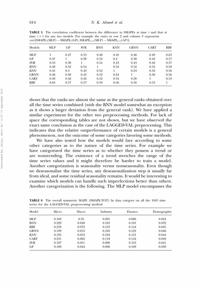
TABLE 5 The correlation coefficient between the difference in SMAPEs at time t and that attime t + 1 for any two models. For example the entry in row 2 and column 3 representscorr

(SMAPEt (MLP) − SMAPEt (GP), SMAPEt+1(MLP) − SMAPEt+1(GP )

)Models MLP GP SVR BNN KNN GRNN CART RBF

MLP 1 0�47 0�53 0�48 0�45 0�46 0�49 0�63GP 0�47 1 0�38 0�52 0�4 0�38 0�42 0�57SVR 0�53 0�38 1 0�54 0�43 0�43 0�42 0�57BNN 0�48 0�52 0�54 1 0�52 0�52 0�52 0�59KNN 0�45 0�4 0�43 0�52 1 0�24 0�34 0�56GRNN 0�46 0�38 0�43 0�52 0�24 1 0�38 0�56CART 0�49 0�42 0�42 0�52 0�34 0�38 1 0�53RBF 0�63 0�57 0�57 0�59 0�56 0�56 0�53 1

shows that the ranks are almost the same as the general ranks obtained overall the time series combined (with the BNN model somewhat an exceptionas it shows a larger deviation from the general rank). We have applied asimilar experiment for the other two preprocessing methods. For lack ofspace the corresponding tables are not shown, but we have observed theexact same conclusion as the case of the LAGGED-VAL preprocessing. Thisindicates that the relative outperformance of certain models is a generalphenomenon, not the outcome of some categories favoring some methods.

We have also tested how the models would fare according to someother categories as to the nature of the time series. For example wehave categorized the time series as to whether they possess a trend orare nontrending. The existence of a trend stretches the range of thetime series values and it might therefore be harder to train a model.Another categorization is seasonality versus nonseasonality. Even thoughwe deseasonalize the time series, any deseasonalization step is usually farfrom ideal, and some residual seasonality remains. It would be interesting toexamine which models can handle such imperfections better than others.Another caregorization is the following. The MLP model encompasses the

TABLE 6 The overall symmetric MAPE (SMAPE-TOT) by data category on all the 1045 timeseries for the LAGGED-VAL preprocessing method

Model Micro Macro Industry Finance Demographic

MLP 0.182 0.35 0.091 0.086 0.024BNN 0.229 0.040 0.103 0.101 0.032RBF 0.232 0.072 0.123 0.144 0.045GRNN 0.199 0.053 0.102 0.122 0.046KNN 0.195 0.053 0.104 0.121 0.044CART 0.231 0.062 0.118 0.144 0.049SVR 0.187 0.051 0.098 0.123 0.041GP 0.189 0.044 0.096 0.109 0.030



case of a zero hidden node network, which essentially means a linearmodel. It might, therefore, be surmised that the superiority of MLPis inherited from its ability to reduce to a linear model. To test thishypothesis, we have categorized the time series into a group where a zerohidden node network is selected (the “Zero-Hid” group) and a groupwhere more hidden nodes are selected (the “Nonzero-Hid” group), asdetermined by the parameter estimation step. Table 7 shows the SMAPE-TOT results for all the aforementioned categorizations for the LAGGED-VAL preprocessing procedures.

One can see that the category-restricted ranking of the models isquite similar to the overall ranking (with the exception of BNN in theseasonal/nonseasonal caregorization). This again indicates that the relativeperformance is broad-based. No specific feature of the time series favors aparticular model. One can observe how the existence of a trend negativelyaffects the performance for all models, and in addition how it accentuatesthe performance differences among the models. One can see that the rankof MLP for the Nonzero-Hid group is still number one, suggesting thatthe superiority of MLP is genuine and not merely due to its ability toswitch to a linear model. However, the relative differences in performancebetween the models in the Nonzero-Hid group get smaller, indicating thatthe other models could possibly benefit if such a switching mechanism isincorporated into them.

To illustrate the presented ideas in a concrete manner, Fig. 4 shows anexample of a time series together with the forecasts of the two models thatachieved the top two spots for this time series, namely MLP and GP. Table 8shows the SMAPE of all the different models for this particular time series.

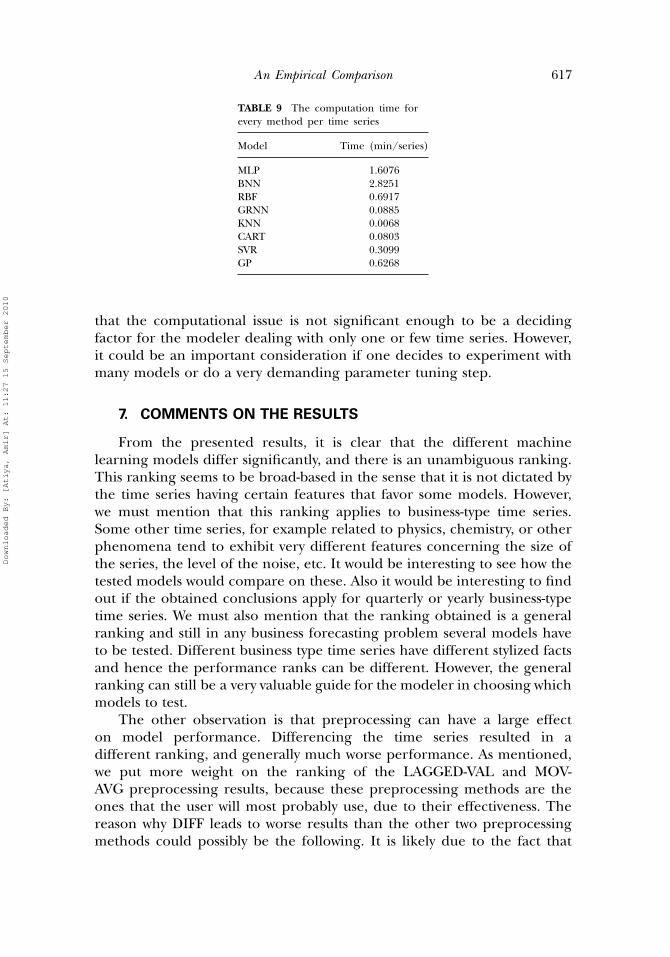
As it turns out, the computational demands of the different modelsvary significantly. Table 9 shows the computation time per time series foreach model. All measurements are based on running the methods onan Intel Centrino Duo 1.83GHZ machine, and using Matlab’s tic andtoc functions. One can see that the most computationally demanding

TABLE 7 The overall symmetric MAPE (SMAPE-TOT) by other categories on all the 1045 timeseries for the LAGGED-VAL preprocessing method

Model Trend No-trend Seasonal Nonseasonal Zero-Hid Nonzero-Hid

MLP 0.1366 0.0597 0.1081 0.0811 0.0848 0.0869BNN 0.1634 0.0716 0.1978 0.0831 0.1078 0.0937RBF 0.2109 0.0803 0.1511 0.1191 0.1304 0.114GRNN 0.1729 0.0689 0.1169 0.1015 0.1087 0.0958KNN 0.1724 0.0683 0.1154 0.1011 0.1084 0.0944CART 0.2043 0.0776 0.1354 0.1175 0.126 0.1104SVR 0.1655 0.0658 0.1113 0.0971 0.1029 0.0935GP 0.1565 0.0631 0.1126 0.0911 0.0981 0.0888



FIGURE 4 The forecasts of the top two models (MLP and GP) for one of the M3 time series.Shown is the training period, followed by the out of sample period (the last 18 points). Theforecasts are shown only for the out of sample period.

model is BNN. Following that comes MLP (as if this is the price one hasto pay for its superior peformance). Following this comes RBF, GP, SVR,CART, then GRNN and KNN, both of which need very little computationtime. At the level of time series lengths we are dealing with here, it seems

TABLE 8 SMAPE for the eightmodels for the time series exampleconsidered in Fig. 4

Model SMAPE

MLP 0.0384BNN 0.0411RBF 0.0442GRNN 0.0513KNN 0.0511CART 0.0566SVR 0.0468GP 0.0397



TABLE 9 The computation time forevery method per time series

Model Time (min/series)

MLP 1.6076BNN 2.8251RBF 0.6917GRNN 0.0885KNN 0.0068CART 0.0803SVR 0.3099GP 0.6268

that the computational issue is not significant enough to be a decidingfactor for the modeler dealing with only one or few time series. However,it could be an important consideration if one decides to experiment withmany models or do a very demanding parameter tuning step.

7. COMMENTS ON THE RESULTS

From the presented results, it is clear that the different machinelearning models differ significantly, and there is an unambiguous ranking.This ranking seems to be broad-based in the sense that it is not dictated bythe time series having certain features that favor some models. However,we must mention that this ranking applies to business-type time series.Some other time series, for example related to physics, chemistry, or otherphenomena tend to exhibit very different features concerning the size ofthe series, the level of the noise, etc. It would be interesting to see how thetested models would compare on these. Also it would be interesting to findout if the obtained conclusions apply for quarterly or yearly business-typetime series. We must also mention that the ranking obtained is a generalranking and still in any business forecasting problem several models haveto be tested. Different business type time series have different stylized factsand hence the performance ranks can be different. However, the generalranking can still be a very valuable guide for the modeler in choosing whichmodels to test.

The other observation is that preprocessing can have a large effecton model performance. Differencing the time series resulted in adifferent ranking, and generally much worse performance. As mentioned,we put more weight on the ranking of the LAGGED-VAL and MOV-AVG preprocessing results, because these preprocessing methods are theones that the user will most probably use, due to their effectiveness. Thereason why DIFF leads to worse results than the other two preprocessingmethods could possibly be the following. It is likely due to the fact that



for many of the considered time series the absolute level is a useful pieceof information. For example there could possibly be some mean revertingbehavior that dictates a more likely reversal direction when high or lowlevels are reached. When choosing between LAGGED-VAL and MOV-AVG,one has to consider the features of the considered time series. For exampleif there is a long term average that is known to have some significance, thenmoving average preprocessing could be a more advantageous method. Ifone would have used lagged preprocessing, then the number of lags couldbe excessive.

The MLP and the GP models are the best two models, with MLP beingthe best for the LAGGED-VAL and MOV-AVG preprocessing methodsand GP being more robust because it did also very well for the DIFFpreprocessing. This is a very interesting result, because GP only veryrecently caught the attention of the machine learning community. It hasbeen developed long time ago, but was never really widely studied orwidely applied until very recently. The MLP model yielded very good resultspartly (but not wholly) because of its ability to reduce to a linear model.This is consistent with one of the conclusions of the M3 competition,which states that simple models tend to outperform more complex models.While support vector machines (SVM) is one of the top models inclassification, in regression it does not seem to keep up the top spot.The BNN is generally similar in performance to SVR. Surprisingly it is inthe second spot in terms of the fraction-best measure, and for MOV-AVGpreprocessing it does very well. Apparently its performance is a bit erratic.For some time series it is in the top position while for others it has ahigh SMAPE. After this comes GRNN and KNN. Their performance is ingeneral average, but they tend to be quite robust, rarely giving bad surprises.GRNN outperforms KNN a little, in general. It is interesting that the threemethods KNN, GRNN and GP are all based on constructing a locally-based weighted average of the target outputs of the training set. Yet, GPoutperforms the other two by so much. Perhaps, this is because GP is basedon a solid probabilistic model. CART gave erratic performance, almostworst performance for the LAGGED-VAL and MOV-AVG preprocessingmethods and almost best performance for the DIFF preprocessing method.Perhaps this is because it does not have enough flexibility as some of theother models with respect to linearly transforming the input space. Theworst model overall is RBF. It consistently gave bad errors. Perhaps the factthat the centers and the kernel widths are not tunable lead it to be tooinflexible.

8. CONCLUSION

We have presented in this work a large scale comparison of eightmachine learning models on the M3 monthly time series of lengths ranging



from 63 to 108 points (for the training period). The machine learningmodels are considered in their basic forms without the modifications andthe additions proposed by so many researchers. The study shows that thereare significant differences between the models, and also that preprocessingcan have a significant impact on performance. The two best models turnedout to be MLP and GP. This is an interesting result, as GP up until fewyears ago has not been a widely used or studied method. We believe thatthere is still room for improving GP in a way that may positively reflect onits performance.

A study that would also be of interest is to extend such a comparisonto more recently developed machine learning models; for example Costilloand Hadi’s (2006) functional networks and White’s (2006) Quicknet. Webelieve comparison studies can guide not only the practitioner in selectingappropriate models, but also the research community in focusing theresearch effort to more feasible or more promising directions.

ACKNOWLEDGMENTS

We would like to acknowledge the help of Athanasius Zakhary of CairoUniversity, who has developed the seasonality test for this work. We alsowould like to acknowledge the useful discussions with Professor Ali Hadi ofthe American University of Cairo and Cornell University and with ProfessorHalbert White of UCSD. This work is part of the Data Mining for ImprovingTourism Revenue in Egypt research project within the Egyptian Data Miningand Computer Modeling Center of Excellence.

REFERENCES

Alon, I., Qi, M., Sadowski, R. J. (2001). Forecasting aggregate retail sales: a comparison of artificialneural networks and traditional methods. Journal of Retailing and Consumer Services 8:147–156.

Alpaydin, E. (2004). Introduction to Machine Learning. Cambridge, MA: MIT Press.Anders, U., Korn, O. (1999). Model selection in neural networks. Neural Networks 12:309–323.Balkin, S. D., Ord, J. K. (2000). Automatic neural network modeling for univariate time series.

International Journal of Forecasting 16(4):509–515.Bishop, C. M. (1995). Neural Networks for Pattern Recognition. Oxford, UK: Oxford University Press.Box, G., Jenkins, G. (1976). Time Series Analysis, Forecasting and Control. San Francisco: Holden-Day Inc.Breiman, L. (1993). Classification and Regression Trees. Boca Raton, FL: Chapman & Hall.Callen, L. J., Kwan, C. C. Y., Yip, P. C. Y., Yuan, Y. (1996). Neural network forecasting of quarterly

accounting earnings. International Journal of Forecasting 12:475–482.Canu, S., Grandvalet, Y., Guigue, V., Rakotomamonjy, A. (2005). SVM and Kernel Methods Matlab

Toolbox. Perception Systèmes et Information, INSA de Rouen, Rouen, France.Caruana, R., Niculescu-Mizil, A. (2006). An empirical comparison of supervised learning algorithms.

Proceedings of the 23rd International Conference on Machine Learning (ICML 2006), June 2006,pp. 161–168.

Castillo, E., Hadi, A. S. (2006). Functional networks. In: Kotz, S., Balakrishnan, N., Read, C. B.,Vidakovic, B., eds. Encyclopedia of Statistical Sciences. Vol. 4. pp. 2573–2583.

Chalimourda, A. Scholkopf, B., Smola, A. J. (2004). Experimentally optimal in support vectorregression for different noise models and parameter settings. Neural Networks 17(1):127–141.



Cherkassky, V., Ma. Y. (2004). Practical selection of SVM parameters and noise estimation for SVMregression. Neural Networks 17(1):113–126.

Cybenko, G. (1989). Approximation by superposition of sigmoidal functions. Mathematics of Control,Signals and Systems 2:303–314.

Foresee, F. D., Hagan, M. T. (1997). Gauss–Newton approximation to Bayesian learning.In Proceedings IEEE Int. Conference Neural Networks, pp. 1930–1935.

Funahashi, K. (1989). On the approximate realization of continuous mappings by neural networks.Neural Networks 2:183–192.

Gencay, R., Qi, M. (2001). Pricing and hedging derivative securities with neural networks: Bayesianregularization, early stopping and bagging. IEEE Transactions on Neural Networks 12:726–734.

Ghysels, E., Granger, C. W. J., Siklos, P. L. (1996). Is seasonal adjustment a linear or nonlineardata filtering process? Journal of Business and Economics Statistics 14:374–386.

Giacomini, R., White, H. (2006). Tests of conditional predictive ability. Econometrica 74:1545–1578.Hardle, W. (1990). Applied Nonparametric Regression, Econometric Society Monographs, 19. Cambridge,

UK: Cambridge University Press.Hastie, T. Tibshirani, R., Friedman, J. (2001). The Elements of Statistical Learning. Springer Series in

Statistics. Springer-Verlag.Hill, T. O’Connor, M., Remus, W. (1996). Neural network models for time series forecasts.

Management Science 42:1082–1092.Hornik, K. Stinchombe, M., White, H. (1989). Multi-layer Feedforward networks are universal

approximators. Neural Networks 2:359–366.Kohavi, R. (1995). A study of cross-validation and bootstrap for accuracy estimation and model

selection. Proceedings International Joint Conference on Artificial Intelligence, IJCAI.Koning, A. J., Franses, P. H., Hibon, M., Stekler, H. O. (2005). The M3 competition: statistical tests

of the results. International Journal of Forecasting 21:397–409.Kwok, J. T. (2001). Linear dependency between and the input noise in support vector regression.

Proceedings of ICANN 2001, LNCS 2130:405–410.Leshno, M., Lin, V., Pinkus, A., Schocken, S. (1993). Multilayer feedforward networks with a

nonpolynomial activation function can approximate any function. Neural Networks 6:861–867.M3 Competition. (2008). http://www.forecasters.org/data/m3comp/m3comp.htm.MacKay, D. J. C. (1992a). Bayesian interpolation. Neural Computation 4:415–447.MacKay, D. J. C. (1992b). A practical Bayesian framework for backpropagation networks. Neural

Computation 4:448–472.Magdon-Ismail, M., Nicholson, A., Abu-Mostafa, Y. (1998). Financial markets, very noisy information

processing. Proceedings of the IEEE 86(11):2184–2195.Makridakis, S., Wheelwright, S. C., Hyndman, R. J. (1998). Forecasting: Methods & Applications, 3rd ed.

Ch. 3, New York: Wiley.Makridakis, S., Hibon, M. (2000). The M3-Competition: results, conclusions and implications.

International Journal of Forecasting 16:451–476.Mattera, D., Haykin, S. (1999). Support vector machines for dynamic reconstruction of a chaotic

system. In: Scholkopf, B. Burges, C., Smola, A., eds. Advances in Kernel Methods: Support VectorLearning. Cambridge, MA: MIT Press, pp. 211–241.

McDonald, B. J., Thompson, W. A. (1967). Rank sum multiple comparisons in one and two wayclassifications. Biometrika 54:487–497.

Medeiros, M. C., Veiga, A. (2000). A hybrid linear-neural model for time series forecasting. IEEETransactions on Neural Networks 11:1402–1412.

Medeiros, M. C., Terasvirta, T., Rech, G. (2006). Building neural network models for time series: astatistical approach. Journal of Forecasting 25:49–75.

Miller, D. M., Williams, D. (2004). Damping seasonal factors: shrinkage estimators for theX-12-ARIMA program. International Journal of Forecasting 20:529–549.

Moody, J. E., Darken, C. (1989). Fast learning in networks of locally-tuned processing units. NeuralComputation 1:281–294.

Moody, J. (1992). The effective number of parameters: An analysis of generalization andregularization in nonlinear learning systems. Advances in Neural Information Processing Systems4:847–854.

Murata, N., Yoshizawa, S., Amari, S. (1993). Learning curves, model selection, and complexity ofneural networks. Advances in Neural Information Processing Systems 5:607–614.



Nadaraya, E. A. (1964). On estimating regression. Theory of Probability and Its Applications 10:186–190.Powell, M. J. D. (1987). Radial basis functions for multivariable interpolation: In: Mason, J. C., Cox,

M. G., eds. A Review in Algorithms for Approximation. Oxford: Clarendon, pp. 143–168.Rasmussen, C. E., Williams, C. K. L. (2006). Gaussian Processes for Machine Learning. Cambridge, MA:

MIT Press.Scholkopf, B., Smola, A. J. (2001). Learning with Kernels: Support Vector Machines, Regularization,

Optimization, and Beyond. Cambridge, MA: MIT Press.Sharda, R., Patil, R. B. (1992). Connectionist approach to time series prediction: An empirical test.

Journal of Intelligent Manufacturing 3:317–323.Smola, A. J., Scholkopf, B. (2003). A Tutorial on Support Vector Regression. NeuroCOLT Technical

Report, TR-98-030.Swanson, N. R., White, H. (1995). A model-selection approach to assessing the information in

the term structure using linear models and artificial neural networks. Journal of Business andEconomic Statistics 13:265–275.

Terasvirta, T., van Dijk, D., Medeiros, M. C. (2005). Linear models, smooth transitionautoregressions, and neural networks for forecasting macroeconomic time series: Areexamination. International Journal of Forecasting 21:755–774.

van Dijk, D., Terasvirta, T., Franses, P. H. (2002). Smooth transition autoregressive models – asurvey of recent developments. Econometric Reviews 21:1–47.

Watson, G. S. (1964). Smooth regression analysis. Sankhy Series A 26:359–372.White, H. (2006). Approximate nonlinear forecasting methods. In: Elliott, G., Granger, C. W. J.,

Timmermann, A., eds. Handbook of Economics Forecasting. New York: Elsevier, pp. 460–512.Zhang, W., Cao, Q., Schniederjans, M. J. (2004). Neural network earning per share forecasting

models: A comparative analysis of alternative methods. Decision Sciences 35(2):205–237.Zhang, G. P., Qi, M. (2005). Neural network forecasting for seasonal and trend time series. European

Journal of Operational Research 160:501–514.


an empirical comparison of machine learning models for time series forecasting

Documents