antibiotics resistance forecasting: a comparison of two
TRANSCRIPT

Antibiotics Resistance Forecasting:A Comparison of Two Time Series Forecast Models
Darja StrahlbergHamburg University of Technology, Germany
Advisors: Prof. Dr. Michael Kolbe, Center for Structural Systems Biology,
University of Hamburg, Germany
Gianni Pagnini, Basque Center for Applied Mathematics & Ikerbasque,
Bilbao, Basque Country - Spain
August 21, 2021
Abstract
The rise of antibiotic resistance is a growing challenge for global health.Antibiotics are used for disease treatment, as well as for medical procedures,for instance, operations and transplants. The aim of this work is to compareauto-regressive integrated moving average (ARIMA) and recurrent neural net-works (RNN) to forecast the spread of drug-resistant bacterial infections at thecommunity level. The comparison of two algorithms is performed for a multi-step time series univariate dataset. Five distinct time series were modelled,each one representing the number of episodes per single ESKAPE infectingpathogen, that has occurred quarterly between 2008 and 2018 calendar yearsin Germany. The forecast quality is evaluated by the root mean squared errorbetween the forecasted values and the test data set. The experimental resultsshow that multi-neural network forecasting RNN is significantly poorer thanARIMA for multi-step forecasting on univariate datasets. Finally, the paperprovides a conclusion, that machine learning complexity is not always addingskill to the forecast. The forthcoming challenges are setting conditions whenmachine learning models can perform well for the real-world applications. Thecode used to evaluate the concept is available.
1 Introduction
The discovery of antibiotics is considered one of the most significant health-relatedevents of the last century. Since the introduction of penicillin, the deployment of anynovel antibiotic has been followed by the evolution of clinically relevant resistance
Copyright © SIAM Unauthorized reproduction of this article is prohibited 383

strains to that antibiotic in as little as a few years [2]. In addition to their use in thetreatment of infectious diseases, antibiotics are critical for the success of advancedsurgical procedures, including organ and prosthetic transplants [4]. So emergingantibiotic resistance is a much broader problem than initially anticipated.
Forecasting the spread of drug-resistant bacterial infections helps in developingcontext-specific national and regional operational plans. The accurate forecast-ing of future behaviour in epidemiology requires efficient mathematical techniques.This paper compares two forecasting techniques for a time series data analysis:auto-regressive integrated moving average (ARIMA) and recurrent neural networks(RNN). Several industries are using classical time series forecasting techniques, likeARIMA, for instance market share pricing for oil industry [11]. Other industriesare using machine learning forecasting techniques, for instance forecasting energyconsumption [6]. So two most popular and widely used techniques from otherindustries have been chosen for a comparison.
The outline of this article is as follows: first, I describe the motivation, then I definethe problem and set a goal for the paper. In Section 2, a brief review of literatureon mathematical models describing disease outbreaks, the main techniques and thelimitations of current approaches are identified. Basic notions of antibiotics resis-tance are presented. Section 3 presents two models for comparison and describesthe details of the simulations setup. It discusses the role of machine learning tech-niques in inferring accurate predictors from observed data. Section 4 presents theresults acquired from the model application to data of the drug-resistant bacterialinfections. Finally, in Section 5, the findings are summarised and a view into futureresearch direction is presented.
1.1 Motivation
Forecasting is the process of making predictions of the future based on past andpresent data. Forecasting of future behaviour in epidemiology is critical for aidingdecision-making by public health officials, commercial and non-commercial institu-tions. The comparison of classical time series forecasting techniques and machinelearning techniques has been done for the stock market analysis [12]. It was ob-served that the machine learning model Bidirectional Long Short-Term memory(BiLSTM) outperformed ARIMA. Additionally, a comparison of the models hasbeen performed for an epidemiological data of influenza in Japan and US [13]. Thecombination of several machine learning algorithms showed consistent performanceimprovements. The outcome of all these studies has been somewhat mixed, butoverall neural networks tended more to outperform classical linear techniques [1].
1.2 Problem Definition
The epidemiological forecasting problem is defined as a time series problem. Thetime series is acquired at discrete times with constant time lag ∆t such that anyacquiring time is ti = i∆t, with i ∈ N. In the following without loss of generality weset ∆t = 1 and then t = i such that t ∈ N and the time series results to be definedby Xt = {x(t = i) = xi | i ∈ N}. The forecast can be written as X̂N+h|N which is theforecast h-steps ahead given the training set N . From above mentioned reasons,
384

these forecast issues have spurred the need for forecasting in order to use the fullcapacity of the available data and be able to plan response activities.
1.3 Goal
The paper focuses on the analysis of medically important drug-resistant bacterialinfections with data gathered by Antibiotics Resistance Surveillance from RobertKoch Institute, Germany [9]. The objective of this analysis is to compare the ac-curacy of the classical time series forecasting method with the machine learningforecast model, and use that information to determine when resistance will rise ordecrease in order to develop an operational plan. The laboratory data were retrievedfrom January 2008 to October 2018, summed per quarter. The total number of datapoints is 44. The forecast has been done for 9-n steps ahead, what is equivalent toa two years forecast.
Here I am running an experiment verification of the proposed methods for forecast-ing drug-resistant bacterial infections. The results are conducted using five bacterialpathogens with increased resistance to commonly used antibiotics to compare ac-curacy of the proposed methods for the forecast of antibiotics resistance in the realenvironment.
2 State of the Art
In the current section a brief review of the literature on different forecast methods isdone by identifying the main techniques and the limitations of current approaches.The section starts with a short introduction into the problem of antibiotic resistance.
2.1 Biological Overview
The current antibiotic crisis can be considered as an evolutionary problem [10]. Bac-teria have a remarkable capacity to adapt and evolve even under extreme conditionsincluding in the Arctic or in boiling water (near ”black smoker” hydrothermal vents).Bacteria can adapt specific genes or even lifestyles in response to the environmentalconditions. Antibiotic resistance has developed to every antibiotic in clinical use,with the resistance genes responsible disseminated globally [5].
The analysis of the infection data offers the capability to potentially forecast therisk of drug-resistant bacterial infections outbreaks. Various attempts were made toinvestigate the development of the antibiotics resistance using different mathematicalmodels on the research objects. For instance, as it is shown in Figure 1: within thepatient, in the hospital or in the community. It is my aim to look at the spread ofthe drug-resistant bacterial infections in the community level.
2.2 Models Overview
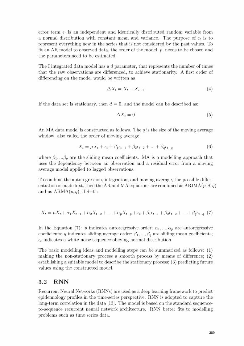
Over the past two centuries the forecasting modelling approaches changed fromdescriptive and dynamic to network and social analysis, as highlighted in Figure 2.The descriptive approach focuses on the general shape and curve prediction based
385
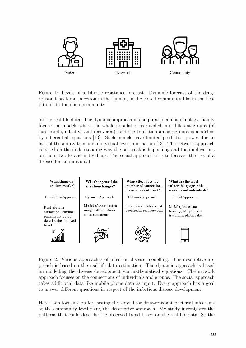
Figure 1: Levels of antibiotic resistance forecast. Dynamic forecast of the drug-resistant bacterial infection in the human, in the closed community like in the hos-pital or in the open community.
on the real-life data. The dynamic approach in computational epidemiology mainlyfocuses on models where the whole population is divided into different groups (ofsusceptible, infective and recovered), and the transition among groups is modelledby differential equations [13]. Such models have limited prediction power due tolack of the ability to model individual level information [13]. The network approachis based on the understanding why the outbreak is happening and the implicationson the networks and individuals. The social approach tries to forecast the risk of adisease for an individual.
Figure 2: Various approaches of infection disease modelling. The descriptive ap-proach is based on the real-life data estimation. The dynamic approach is basedon modelling the disease development via mathematical equations. The networkapproach focuses on the connections of individuals and groups. The social approachtakes additional data like mobile phone data as input. Every approach has a goalto answer different questions in respect of the infectious disease development.
Here I am focusing on forecasting the spread for drug-resistant bacterial infectionsat the community level using the descriptive approach. My study investigates thepatterns that could describe the observed trend based on the real-life data. So the
386

epidemiological problem of the future number of cases of the drug-resistant bacterialinfection can be defined as a time series problem.
Definition 1 A time series is a sequence of observations xt, where t ∈ N collectedat equal spaced, discrete time intervals.
Forecast of time series data is to model the future state as a combination of past datapoints [13]. The classical model considers the future state as a linear combination ofpast data, whereas machine learning models considers the future state as a non-linearcombination of past data.
Classical Model. The general model for time series can be written as
xt = g(t) + εt; t = 1, ..., T (1)
where T is the number of observations, g(t) is a deterministic function of time, εt aresidual term, or a noise, which follows a probability law.
In the time series analysis, it is assumed that the data (observations) consist of asystematic pattern and stochastic component; the former is deterministic in nature,whereas the latter accounts for the random error and usually makes the patterndifficult to be identified. The stochastic component of the time series is describedby the error term εt. The basic assumption in time series analysis is that someaspects of the past pattern will continue to remain in the future [14]. It is necessaryto evaluate if the time series components are time invariant, meaning the componentsare constant. It is assumed that the error distribution is the same by every datapoint: εt ∼ N(0, σ2), where N is the normal density with zero mean and varianceσ2. So, in this case the distribution still will be normal, and that its mean and thevariance will still be the same 0 and σ2. It demonstrates the invariant part of theprocess. So the goal is to find something invariant, which was the distribution oferrors. The stationary series by definition have invariant parts such as unconditionalmean and variance.
Machine Learning Model is an umbrella term for techniques that fit models algo-rithmically by adapting to patterns in data [8]. The prediction problem is defined asa problem of supervised learning problem. Possible non-linear dependence betweenthe input (past embedding vector) and the output (future value) is attempted. Theforecast is usually based on the idea according to which reliable predictions canbe obtained solely on the grounds of our knowledge of the past. Chaos is oftenconsidered the main limiting factor to predictability in deterministic systems. [7,S. 567]
The representation of unknown input/output relation can be written as follows
y = f(x) + w (2)
where f(x) is a deterministic function, and the term w represents the random error.
The data are restricted to look like a supervised learning problem. The previoustime stamp is an input variable x and the next step as the output variable y. Twohypotheses, which are seldom made explicitly, are needed to articulate an affirmative
387

answer: 1. Similar premises lead to similar conclusions (Analogy); 2. Systems whichexhibit a certain behaviour will continue doing so (Determinism) [7]. The main limitto predictions based on analogues is not the sensitivity to initial conditions, typicalof chaos. But, the main issue is actually to find good analogs [7].
Big data undoubtedly constitute a great opportunity for scientific and technologicaladvance, with a potential for considerable socio-economic impact. To make themost of it, however, the ensuing developments at the interface of statistics, machinelearning and artificial intelligence, must be coupled with adequate methodologicalfoundations, not least because of the serious ethical, legal and more generally societalconsequence of the possible misuses of this technology [7].
I have given a biological and models overview. For the next step, I am going tocompare two models of forecasting the spread for drug-resistant bacterial infectionsat the community level: the classical model with ARIMA and the machine learningmodel with RNN.
3 Methodology
In this section the time series analysis of drug-resistant bacterial infection data willbe used to make a forecast with two models: ARIMA and RNN.
The goal is to obtain a 9-step ahead forecast to test the forecasting performance ofthe ML method for a long horizon. Two methods are going to be compared on thesame data set: the classical time series forecasting model ARIMA and the machinelearning time series forecasting model RNN. The basic idea of ARIMA is to modelthe future state as a linear combination of past data points, whereas the basic ideaof RNN is to model the future state as a non-linear combination of past data points.
3.1 ARIMA
In this section an overview of the theoretical explanation of the ARIMA model isgiven.
The current problem is defined as a regression problem, the output variable is areal value. The ARIMA model is a parametric method which represents data pointsas a linear combination of its previous values plus an error term. The approach isto model drug-resistant bacterial infection as time-series patterns with the ARIMAmodel. The model consists of three components: auto regressive (AR), integrated(I) and moving average (MA) models. As it was described above, it is importantto evaluate if the time series components are time invariant, meaning the process isstationary.
An AR data model with p terms is constructed as follows, where p is the number ofautoregressive terms included in the model; for a time series Xt
Xt = µ+ α1Xt−1 + α2Xt−2 + ...+ αpXt−p + εt (3)
where µ is the mean value, αt is the weight of the correlation coefficients that ismultiplied with the lagged values of Xt and t is the number of observations. The
388
error term εt is an independent and identically distributed random variable froma normal distribution with constant mean and variance. The purpose of εt is torepresent everything new in the series that is not considered by the past values. Tofit an AR model to observed data, the order of the model, p, needs to be chosen andthe parameters need to be estimated.
The I integrated data model has a d parameter, that represents the number of timesthat the raw observations are differenced, to achieve stationarity. A first order ofdifferencing on the model would be written as
∆Xt = Xt −Xt−1 (4)
If the data set is stationary, then d = 0, and the model can be described as:
∆Xt = 0 (5)
An MA data model is constructed as follows. The q is the size of the moving averagewindow, also called the order of moving average.
Xt = µXt + εt + β1εt−1 + β2εt−2 + ...+ βqεt−q (6)
where β1, ...βq are the sliding mean coefficients. MA is a modelling approach thatuses the dependency between an observation and a residual error from a movingaverage model applied to lagged observations.
To combine the autoregression, integration, and moving average, the possible differ-entiation is made first, then the AR and MA equations are combined as ARIMA(p, d, q)and as ARMA(p, q), if d=0 :
Xt = µXt +α1Xt−1 +α2Xt−2 + ...+αpXt−p + εt + β1εt−1 + β2εt−2 + ...+ βqεt−q (7)
In the Equation (7): p indicates autoregressive order; α1, ..., αp are autoregressivecoefficients; q indicates sliding average order; β1, ..., βq are sliding mean coefficients;εt indicates a white noise sequence obeying normal distribution.
The basic modelling ideas and modelling steps can be summarized as follows: (1)making the non-stationary process a smooth process by means of difference; (2)establishing a suitable model to describe the stationary process; (3) predicting futurevalues using the constructed model.
3.2 RNN
Recurrent Neural Networks (RNNs) are used as a deep learning framework to predictepidemiology profiles in the time-series perspective. RNN is adopted to capture thelong-term correlation in the data [13]. The model is based on the standard sequence-to-sequence recurrent neural network architecture. RNN better fits to modellingproblems such as time series data.
389

A neural network takes an independent variable X (or a set of independent variables )and a dependent variable y, then it learns the mapping between X and y (Training).Once training is done, a new independent variable can be given to predict thedependent variable.
The RNN has sequential input, sequential output, multiple timesteps, and multiplehidden layers. The Figure 3 highlights how RNN works. I calculate hidden layervalues not only from input values but also previous time step values and Weights(W) at hidden layers are the same for time steps.
Figure 3: Description of the RNNs. U - Weight vector for hidden layer, V -weightvector for output layer, W - same vector for different time steps, X- Infection oc-currences vector for input, Y - Drug-resistant bacterial Infections for output
The steps for the forecast are described described below.
3.3 Steps in Forecasting
The forecasting process involves the choice of the model, data splitting, fitting themodel, model evaluation, re-fitting the model on the entire data set and forecast ofthe future behaviour. Figure 4 highlights the steps for a forecasting model. Eachstep will be further described. The output of the forecast is the number of drug-resistant bacterial infections towards a specific antibiotic at each time step.
Data Split. By convention, the test interval does not exceed 20% of the availabledata. So if the total available data set has 44 data points, then the test data set is9 data points, which is equivalent to 9 quarters or 2 years. The training data setconsists of 35 data points, what is approximately 9 years of observation.
390

Figure 4: The forecasting process consists of several steps: 1) the choice of the modelbased on the available data, 2) data split into training and test data sets, usuallywith the ratio 80:20, 3) the model is fit on the training data set, 4) model evaluationwith RMS error, 5) the model is re-fitted on the whole data set, 6) forecast for futuren-steps of data points.
If the dataset is denoted as x1, x2, ..., xN , then the training dataset has the lengthT= 35 and denoted as x1, x2, ..., xT . The test dataset has the length h = 9 datapoints and denoted as xT+1, ..., xN . In this example the test dataset and forecastdataset are equally long.
Fit model on training set. The parameters for the ARIMA model need to bechosen correctly, for (p, d, q). The parameters depend on the individual data char-acteristics. The RNN model requires weight function estimation to be performed.The model is initially fit on a training dataset or trained, meaning that the modelis learning from the training data set.
Evaluate model on test set. The new segment Yt is obtained with the ARIMAmodel. Yt has the same length as the test data set Xt. During the process ofprediction, the expectation is to obtain the best prediction value with no error orthe smallest possible error, that is, to obtain the best future prediction value usingroot mean square error minimization. Root mean square error (RMSE) is definedas the root mean square of the ARIMA prediction and the actual value, during thetime interval h, which denoted as
λ =
√√√√ 1
N
N∑t=1
(Xt − Yt)2 (8)
where Yt indicates the predicted value, Xt indicates the true value from the testdata set and N is the sequential number of steps in time in the time interval h.
391

Re-fit model on entire data set If the dataset is denoted as x1, x2, ..., xN , thetraining data is set as an entire data set x1, x2, ..., xN .
Forecast for future data The prediction interval should not be longer than thetest interval. So the prediction interval is 8 data points, 8 quarters or 2 years. Themodel is trained on the entire data set of the length N . So the training data setshould be at length at least N=44, for a forecast of h =8 data points - quarters -ahead.
Two time series forecasting models and steps of the forecasting process have beendescribed. An experimentation comparison of the proposed methods for time seriesforecasting of the drug-resistant bacterial infectious disease is presented in the nextsection. The implementation of the proposed methods for the forecasting and resultsare shown in detail.
4 Use Case: ESKAPE bacteria
I have tested the forecasting models on the data of drug-resistant bacterial infections.The code used to evaluate the concept can be found on the github in [3]. I haveused data of five highly relevant bacterial pathogens known as ESKAPE.
4.1 Available Data
ESKAPE is an acronym encompassing the names of six highly important bacterialpathogens commonly associated with antimicrobial resistance. Medically impor-tant bacteria include the following pathogens: Enterococcus faecium, Staphylococcusaureus, Klebsiella pneumoniae, Acinetobacter baumannii, Pseudomonas aeruginosaand Enterobacter species.
This study was conducted using data exported from the Antibiotics ResistanceSurveillance from the Robert Koch Institute. Laboratories from all of Germanyreport these data on a regular basis [9]. The data are not differentiated by theregion. Data used in this study included the time (quarter), the number of testedpathogens with confirmed resistance to a specific antibiotic. The laboratory datawere collected from January 2008 to October 2018, summed per quarter. Thus, thedata utilized for the analysis included quarter time series of isolates of E. faeciumwith Vancomicyn resistance, S. aureus with Penicillin resistance, K.pneumoniaewith Amikacin resistance, A. baumannii with Imipenem resistance, P. aeruginosawith Imipenem resistance. The time series of Enterobacter were not available.
The forecast is the multiple-step-ahead forecast, for 9-n future steps. Forecast ac-curacy was assessed for each each time series. The data were treated as individualtime series, analysed and evaluated separately.
4.2 Implementation
Implementation is showed in detail on bacteria A. baumannii with Imipenem re-sistance. Further ESKAPE bacteria pathogens have been analysed with the samestrategy. Results are featuring analysis of the data sets from all bacteria pathogens.
392

Data Pre-processing Preliminary descriptive analysis was conducted at first.My aim is to identify relevant features, such as autocorrelation, seasonal patterns,trends, and any other notable fluctuations. Each time series was evaluated to de-termine whether it was stationary (i.e. whether basic statistical properties suchas mean and variance of the series remained constant through time). Initial dataanalysis was conducted via computational tests of basic descriptive statistics.
The properties of this dataset are as follows:
• This is a real life dataset acquired from Antibiotics Resistance Surveillancefrom the Robert Koch Institute. The process is realistic. The quality of themonitoring data is high.
• The dataset consists of 44 data points, which were collected over the years fromLaboratories in Germany. The data set contains observations from severallaboratories.
• Each data point indicates the number of drug-resistant bacterial infectionssummed during three months.
• The dataset is not stationary.
• The dataset is univariate - one variable data input.
Data Split. The training data set is 35 quarter data points. The test data set is 9data points. The ARIMA model and RNN use time series data as input. The dataare reported in Figure 5 for the bacteria A. baumannii.
Figure 5: Drug-resistant bacterial infections from bacteria A. baumannii with Imip-inem resistance over the period of 10 years. The blue line represents the training data set of 34 data points and the orange line represents the test data set of 9 data points.
Fit model on training set. From the above analysis the data set is qualified to be
393
modelled by ARIMA(p, d, q). The parameters have been estimated via computation((p, d, q)) = (6,0,0)). These parameter values were also confirmed programmaticallyusing the exhaustive grid search optimisation. Parameters have been estimatedseparately for each time series data set.
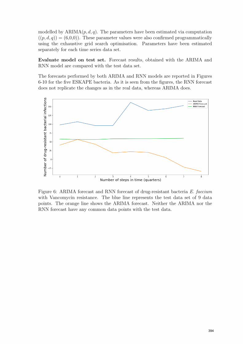
Evaluate model on test set. Forecast results, obtained with the ARIMA andRNN model are compared with the test data set.
The forecasts performed by both ARIMA and RNN models are reported in Figures6-10 for the five ESKAPE bacteria. As it is seen from the figures, the RNN forecastdoes not replicate the changes as in the real data, whereas ARIMA does.
Figure 6: ARIMA forecast and RNN forecast of drug-resistant bacteria E. faeciumwith Vancomycin resistance. The blue line represents the test data set of 9 datapoints. The orange line shows the ARIMA forecast. Neither the ARIMA nor theRNN forecast have any common data points with the test data.
394
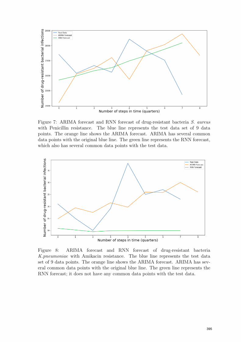
Figure 7: ARIMA forecast and RNN forecast of drug-resistant bacteria S. aureuswith Penicillin resistance. The blue line represents the test data set of 9 datapoints. The orange line shows the ARIMA forecast. ARIMA has several commondata points with the original blue line. The green line represents the RNN forecast,which also has several common data points with the test data.
Figure 8: ARIMA forecast and RNN forecast of drug-resistant bacteriaK.pneumoniae with Amikacin resistance. The blue line represents the test dataset of 9 data points. The orange line shows the ARIMA forecast. ARIMA has sev-eral common data points with the original blue line. The green line represents theRNN forecast; it does not have any common data points with the test data.
395

Figure 9: ARIMA forecast and RNN forecast of drug-resistant bacteria A. baumanniiwith Imipenem resistance. The blue line represents the test data set of 9 data points.The orange line shows the ARIMA forecast. ARIMA has several common data pointswith the original blue line. The green line represents the RNN forecast; it does nothave any common data points with the test data.
Figure 10: ARIMA forecast and RNN forecast of drug-resistant bacteria P. aerugi-nosa with Imipenem resistance. The blue line represents the test data set of 9 datapoints. The orange line shows the ARIMA forecast. The green line represents theRNN forecast; the RNN forecast has more data points in common with the test datathan the ARIMA forecast.
4.3 Results
Two different time series forecasting method have been evaluated by the accuracyof the prediction.
396

Accuracy. Table 1 reports the Rooted Mean Squared Error (RMSE) achieved byeach technique for forecasting the drug-resistance bacteria infection data. In threeout of five test cases, ARIMA performs better then RNN. In particular, the RMSEfor bacteria A. baumannii is λ =8.0 for ARIMA(6, 0, 0) and λ =12.0 and for theRNN model. The similar difference in the RMSE is for the bacteria K.pneumoniae.The RMSE of ARIMA for the bacteria S. aureus is λ =1221.5, whereas the RMSEof RNN is λ =1416.6.
For two bacteria E. faecium and P. aeruginosa the RNN model has shown betterresults than the ARIMA model. The RMSE of the RNN model for the bacteriaP. aeruginosa is λ =137.7, what is half of the RMSE of the ARIMA model withλ =273.9. The RNN model has performed significantly better for the bacteria E.faecium as well. As the data characteristics of the bacteria data are the same, it ishard to say why the results in the quality of the forecast differ so much.
Table 1: RMSEs of ARIMA and RNN
Bacterial pathogen ARIMA RNNE. faecium withVancomycinresistance
114.5 79.0
S. aureus withPenicillin resistance
1221.5 1416.6
K.pneumoniaewith Amikacinresistance
5.9 12.5
A. baumannii withImipenemresistance
8.0 12.0
P. aeruginosa withImipenemresistance
273.9 137.7
4.4 Discussion
Our results suggest that machine learning methods do not always perform well asexpected.
The observations describing the results are the follows:
1. Out of five time series data sets the ARIMA forecast model showed betterperformance for three data sets. The forecasting accuracy of the machinelearning RNN model does not prove to be always significantly better as tothat of ARIMA model for multi-step forecasting on univariate datasets. Thiswork demonstrates that machine learning complexity is not always adding skillto the forecast. The potential reason is that RNN cannot preserve and thusdoes not remember long inputs [12]. Another hypothesis is that additionaldata preparation is required.
397

2. The RNN forecast model outperforms the classical ARIMA model for two datasets. As all five data sets have similar data characteristics, it is hard to say whythe forecast accuracies are so different. This work demonstrates that there isno standard solution even for the similar datasets.
3. ARIMA requires the time series input only. This feature makes it relativelyeasy to implement, without high additional costs.
5 Conclusion
The purpose of this paper is to compare classical time series forecasting models withmachine learning models on the real-life data of drug-resistant bacterial infectiondevelopment. The classical time series models, such as ARIMA, models the futurestate as a linear combination of past data points. On the contrary, Machine Learningmodel such as RNN model the future state as a non-linear combination of past datapoints.
The paper was approached in the following steps:
Step 1. Define antibiotic resistance forecast problem at the community level astime series multi-step forecast problem.
Step 2. Check the available methods in the classical time series analysis and ma-chine learning analysis.
Step 3. Forecast antibiotics resistance at the community level.
ARIMA and RNN were chosen as methods to forecast the number of drug-resistantbacterial infection occurrences with resistance. Forecast modelling was performedfollowing the six steps: choose model, split data into train and test data, fit model ontraining set, evaluate model on test set, re-fit model on entire data set and forecastfor future data.
Step 4. Experiment on the ESKAPE infection occurrences with resistance
The experiment included the data collection from Antibiotics Resistance Surveillancefrom the Robert Koch Institute for 10 years, as per the six steps indicated above.The results show that the ARIMA model performed well for three out of five datasets. Thus it can be seen that the RNN model does not perform well for multi-stepforecasting on univariate datasets even when the data sets have similar properties. Itcan be explained by the fact that RNN cannot preserve and thus does not rememberlong inputs.
Future work can be concentrated on the combination of different machine learningmethods and understanding in what cases the machine learning models deliver betterresults.
The results obtained by the forecast of drug-resistant bacterial infection occurrencesare specific to a data set and should not be extrapolated to other data sets without
398
previous verification. However the approach proposed in this paper for forecastingmay be considered equally valid for other epidemiological data.
References
[1] Nesreen K. Ahmed et al. “An Empirical Comparison of Machine LearningModels for Time Series Forecasting”. In: Econometric Reviews 29.5-6 (2010),pp. 594–621. issn: 0747-4938. doi: 10.1080/07474938.2010.481556.
[2] Anne E. Clatworthy, Emily Pierson, and Deborah T. Hung. “Targeting viru-lence: a new paradigm for antimicrobial therapy”. In: Nature Chemical Biology3.9 (2007), pp. 541–548. issn: 1552-4450. doi: 10.1038/nchembio.2007.24.
[3] Darja Strahlberg. GitHub Repository. url: https://github.com/DarjaStrahl/AntibioticResistance_Comparison.git.
[4] Julian Davies and Dorothy Davies. “Origins and evolution of antibiotic resis-tance”. In: Microbiology and Molecular Biology Reviews : MMBR 74.3 (2010),pp. 417–433. doi: 10.1128/MMBR.00016-10.
[5] Ayari Fuentes-Hernandez et al. “Using a sequential regimen to eliminate bac-teria at sublethal antibiotic dosages”. In: PLoS Biology 13.4 (2015), e1002104.doi: 10.1371/journal.pbio.1002104.
[6] G. E. Nasr, E. A. Badr, and and M. R. Younes. “Neural Networks in Fore-casting Electrical Energy Consumption”. In: FLAIRS-01 Proceedings, AAAI(2001).
[7] Hykel Hosni and Angelo Vulpiani. “Forecasting in Light of Big Data”. In:Philosophy & Technology 31.4 (2018), pp. 557–569. issn: 2210-5433. doi: 10.1007/s13347-017-0265-3.
[8] Stephen J. Mooney and Vikas Pejaver. “Big Data in Public Health: Terminol-ogy, Machine Learning, and Privacy”. In: Annual Review of Public Health 39(2018), pp. 95–112. doi: 10.1146/annurev-publhealth-040617-014208.
[9] Robert Koch Institute. Antibiotika Resistenz Surveillance Datenbank. url:https://ars.rki.de/Content/Database/Introduction/Main.aspx.
[10] Roderich Roemhild and Hinrich Schulenburg. “Evolutionary ecology meetsthe antibiotic crisis: Can we control pathogen adaptation through sequentialtherapy?” In: Evolution, Medicine, and Public Health 2019.1 (2019), pp. 37–45. issn: 2050-6201. doi: 10.1093/emph/eoz008.
[11] Ron Alquist, Lutz Kilian, and Robert J. Vigfusson. “Forecasting the Price ofOil”. In: Bank of Canada Working Paper (2011).
[12] Sima Siami-Namini, Neda Tavakoli, Akbar Siami Namin. “A comparativeAnalysis of Forecasting Financial Time Series Using ARIMA, LSTM, and BiL-STM”. In: arXiv preprint arXiv:1911.09512 (2019).
[13] Yuexin Wu et al. Deep Learning for Epidemiological Predictions. 2014. url:http://arxiv.org/pdf/1406.1078v3.
[14] Yufeng Yu et al. “Time Series Outlier Detection Based on Sliding WindowPrediction”. In: Mathematical Problems in Engineering 2014.2 (2014), pp. 1–14. issn: 1024-123X. doi: 10.1155/2014/879736.
399