An Electrophysiologist’sIntroduction to Matlab

— with Examples and Exercises —

Daniel A. Wagenaar and Michael Wright

First presented at: Neural Systems and Behavior Course,Marine Biological Laboratory, Woods Hole, MA, June 2008.

Revised annually for the 2009–2018 courses.

(C) 2008–2018 Daniel Wagenaar and Michael Wright. All rights reserved. You may freely distributethis document in whole or in part and use it in teaching, provided that you properly attribute it byleaving this copyright notice intact. Many of the examples in this document require a Matlab toolboxcalled “WagenaarMBL”, which you may download from http://www.danielwagenaar.net/teaching.On that website you can also find the latest version of this document.

Introduction

GOAL: The main goal for today’s lab is to give you an introduction to the Matlab programmingenvironment. You will then use Matlab to analyze the electrophysiological data you collect later in theday. Although you have been using Matlab for the previous exercises, here we want you to explore moreof the ins ’n’ outs of the program.

Matlab is an interpreted1 computer language intended for data analysis. At first, you don’t reallyhave to know that it is a full-fledged computer language, because it can be used like a basic calcu-lator that can also generate graphs. Over time, you will appreciate how well Matlab handles largedata sets, and how easy it is to add your own data analysis functionality to what comes standard.An introduction to Matlab could easily fill a semester-long course at a university, because the capa-bilities of the system are very wide-ranging. We don’t have that much time, so we’ll just cover thevery basics, and then proceed to some applications you will need for analysis of electrophysiologicaldata. The style of this introduction is rather concise; it is our hope that this will allow you to quicklylearn the essentials without getting bogged down in details. For those of you who are unfamiliarwith Matlab, Chapter 1 will provide a gentle introduction to working with the program; those ofyou more familiar with Matlab may find that the rest of the introduction adds to your knowledgeof Matlab. Several more extensive introductory texts are available on the Internet (as well as inbookstores). The following are still available as of May 2017:

• “Numerical Computing with MATLAB”: A several-hundred-pages-long text book by CleveMoler, the president of Mathworks (the company that produces Matlab):

http://www.mathworks.com/moler/chapters.html.

• “An Introduction to Matlab”: A shorter introduction by David F. Griffiths of the University ofDundee; similar in style to the text you are reading, but quite a bit longer:

http://www.maths.dundee.ac.uk/software/MatlabNotes.pdf.

• “Introduction to Matlab”2: Another fairly short introduction, by Anthony J. O’Connor of Grif-fith University, Brisbane, Australia:

https://maxwell.ict.griffith.edu.au/spl/matlab-page/matlab tony.pdf.

There are also many books published about Matlab. Here are just a few, selected by MW:

• “Mastering Matlab” by Hanselman and Littlefield. This book provides the most in-depth cov-erage of Matlab. There are plenty of worked examples, as well.

1“Interpreted” in this context means that you can type commands and get immediate responses. This is in oppositionto “compiled” languages, which execute faster, but make program development much harder.

2for some reason, cutting and pasting this link in a web browser will not bring up the .pdf file; however, a googlesearch for ”connor matlab griffith” will bring up the pdf file as the first hit

2

• “Getting Started with Matlab” by Rudra Pratap. This book provides a very gentle yet thoroughhandling of Matlab.

• “Essential Matlab for Scientists and Engineers” by Brian Hahn. An intermediate-level bookthat focuses more on doing.

• “Matlab: An Introduction With Applications” by Amos Gilat. Another intermediate-level bookwith a lot of worked examples.

In MW’s experience, Mastering Matlab has been the most helpful, but it assumes you know whatyou want to do. Outside of that, individual books focus on different aspects of Matlab and as suchMW tends to use a combination of books like Pratap and Hahn3 in addition to Hanselman andLittlefield. DAW likes to point out that the online help system is also very extensive and answersmany questions. You may also look into the book “Matlab for Neuroscientists,” by Wallisch et al.,Academic Press, 2008.

As you work your way through this tutorial, we strongly encourage you to experiment with eachof the examples: try variations on them; find out what works and what doesn’t. You really can’tdamage anything by typing nonsense at a computer (unless you try hard: the “delete” command,for instance, is predictably dangerous). If you get stuck, try typing “help”. To learn more aboutMatlab’s online help system, type “help help”. You get the picture. There is also an extensive“help browser” built into Matlab; this you can access from the top menu bar or by typing “doc”.

In the following, text you type at the keyboard is typeset like this; answers given by Matlabare typeset like this.

3If those two are not to your liking, you may take a look at McMahon’s “Matlab Demystified”

3

Chapter 1

Introduction to the basics of thelanguage

This chapter teaches you how to use Matlab to perform simple calculations and to draw graphs.Not much in this chapter is specifically geared toward handling electrophysiological data, but evenif you are eager to start analyzing your recently acquired data, working your way through theexamples and exercises in this chapter will hopefully pay off: they will provide you with a workingknowledge of Matlab, which will not only greatly facilitate understanding the later chapters, butwill also allow you to tailor the examples presented there to your specific needs.

1.1 Basic mathematics

1.1.1 Arithmetic

Addition, subtraction, multiplication, division, and exponentiation are written as you would expect:“+”, “-”, “*”, “/”, “ˆ”. Multiplication and division take precedence over addition and subtraction,and exponentiation takes precedence over all. Parentheses can be used to enforce interpretation.Large and small numbers can be written in exponential notation, e.g., “5e-3” means 0.005.

Example 1>> 1+2*5

ans =

11

>> (1+2)*5

ans =

15

>> 7*3ˆ2

ans =

63

>> 5e-2/7.0e3

ans =

7.1429e-06

You see that Matlab announces that it is ready for your input by showing its “>>” prompt, and thatit prefixes its answers by the text “ans =”. (If you are using the student version of Matlab, theprompt is “EDU>>” instead of plain “>>”.)

Exercise 1How would you ask Matlab to compute

4× 2

3 + 5?

4

1.1.2 Mathematical functions

Matlab defines a long list of mathematical functions (plus you can define your own; see below).

Example 2>> cos(60*pi/180)

ans =

0.5000

>> log(10)

ans =

2.3026

Exercise 2Can you make Matlab confirm that

√2 is about 1.41? Hint: There is a function called

“sqrt”. Find out about it by typing “help sqrt” or “doc sqrt”.

1.1.3 Logic and comparisons

Comparison between numbers in Matlab is expressed using “==”, “>”, “<”, “>=”, and “<=”. Notethat equality is tested using two equals signs. A single equals sign expresses variable assignment;see below. Matlab represents truth as “1” and falsehood as “0”. Logical “and” is written as “&”;logical “or” as “|”.

Example 3>> 2 > 1

ans =

1

>> 3 == 7

ans =

0

>> 5 > 3 & 5 < 8

ans =

1

>> 5 = 3

??? 5=3|

Error: Incorrect use of ’=’operator. [...]

Exercise 3Which is bigger, 37 or 74? Hint: You could just ask Matlab to compute the two numbersseparately, and do the comparison yourself, but that’s not the point of the exercise.

1.2 Creating and using variables

Names of variables in Matlab can have any length, and may contain letters, numbers, and under-scores. They must start with a letter. Assignment is written as “=”.

Example 4>> x = 5

x =

5

>> y = 3 * xˆ2

y =

75

5

Exercise 4What happens if you redefine a variable? Do other variables automatically change theirvalues to match (as in the neural simulator Neuron), or do they remain unaffected (asin the programming languages Java or C)?

If you don’t want to see intermediate results, simply place a semicolon at the end of a line. To showthe value of a variable, simply type its name.

Example 5>> spd = 8;>> dur = 7;>> dist = spd*dur;

>> dist

dist =

56

Exercise 5Can you think of a reason why this is useful? (Hint: Try example 13 below withoutsemicolons.)

Matlab calls the collection of all currently defined variables your “workspace.” An overview ofyour current workspace is shown in (and can be explored from) a separate panel of Matlab’s mainwindow.

1.2.1 Structured variables

It is possible to store variables inside variables. This can greatly help to preserve clarity when usinga large number of variables.

Example 6>> x.a = 3;>> x.b = 7;>> y = x

y =

a: 3b: 7

Exercise 6Can you apply this technique recursively? In other words, what happens if you try tostore a structured variable inside another variable? (Try it by typing “rr.xx = x” fol-lowing the previous example.)

1.3 Using vectors and matrices

Matlab derives its name from the fact that it is very good at handling matrices. Variables canrepresent matrices just as easily as they can represent simple numbers (sometimes called “scalars”when contrasting them against vectors or matrices). Arithmetic and mathematical operations canbe performed just as easily on matrices as on numbers.

6

1.3.1 Defining matrices

Matrices are defined by putting a series of numbers (or variables) in square brackets. Rows of thematrix are separated by semicolons.

Example 7>> x = [ 1 2 3 ]

x =

1 2 3

>> xx = [x 4 5 6]

xx =

1 2 3 4 5 6

>> xxx = [x; 7 8 9]

xxx =

1 2 37 8 9

>> y = [ 2; 4; 6]

y =

246

(Note that some people to prefer to place commas between values in a horizontal row of a matrix.Those are optional.)As the example suggests, more often than true matrices (which are two-dimensional arrays ofnumbers), we will use one-dimensional arrays, or vectors. Matlab treats them all the same; a vectorof length N is just a matrix of size 1xN (as in the case of x in the example) or Nx1 (as in the caseof y).

Exercise 7In example 7, we concatenated the vector “[7 8 9]” to the vector “x” to generate“xxx”. Can you concatenate “[7 8 9]” to the vector “y” from the example? Why(not)? How about concatenating “[7; 8; 9]” to “y”?

1.3.2 Arithmetic on matrices

Matrices may be added to each other or multiplied by scalars using the same operators used forsimple numbers. This only works for matrices that have the same size.

Example 8 (Continued from previous example.)>> z = 2 * x

z =

2 4 6

>> w = x + z + 1

w =

4 7 10

Exercise 8Can you apply mathematical functions to matrices? Create a matrix that contains thenumbers 0, π/6, π/4, π/3 and π/2 (which in radians correspond to 0◦, 30◦, 45◦, 60◦,and 90◦), and calculate their sines and cosines. Does the answer make sense?

Confusingly, to multiply matrices element-by-element, you cannot use the operator “*”, since thatrepresents matrix multiplication. Instead, you must write “.*”. Similarly, “/” represents multiplica-tion by the matrix inverse, and “ˆ” represents matrix exponentiation (which you almost certainlywill never use). Instead, write “./” and “.ˆ”. If you accidentally write “*” (or “/”, etc.) where“.*” (or “./”, etc.) would be appropriate, you may get unexpected results or error messages. For-tunately, it is never an error to write “.*”, even when multiplying simple numbers.

7

Example 9>> [4 6 15] ./ [2 3 5]

ans =

2 2 3

>> [1 2] * [1; 2]

ans =

5>> [1; 2] * [1 2]

ans =

1 22 4

>> [1 2] * [ 1 2]??? Error using ==> *Incorrect dimensions for matrix

multiplication. [...]

>> 5 .* 7

ans =

35

Note: If you do not know what “matrix multiplication” means, don’t worry; you won’t be needingit in this course. A simple working strategy is to write “.*” and “./” instead of “*” and “/” unlessyou have a specific reason not too.

Exercise 9Construct a matrix named “x2” the elements of which are the squares of the elementsof the matrix “xxx” in Example 7.

1.3.3 Accessing the contents of matrices

The examples above show how Matlab can perform arithmetic on all the elements of a matrix atonce. What if you want to work with specific elements? The examples below show how to do that.

Example 10>> x = [2 4 6 8 10];>> x(4)

ans =

8

>> k = 3;>> x(k) = 0

x =

2 4 0 8 10

>> y = [2 4; 6 8]

y =

2 46 8

>> y(2,1)

ans =

6

Exercise 10What happens if you try to access an element that does not exist, such as “x(7)” inthe previous example? What if you accidentially treat a matrix as a vector or vice versa,e.g., by asking for “y(2)” or “x(2,2)” in the previous example? Do you understandhow Matlab treats those ill-formed inputs?

1.3.4 Matrices inside structured variables

The ability to hold multiple variables inside another variable is especially useful with matrices. Forinstance, you might like the variable “spk” to represent a series of action potentials, and you wantto have it store the times of the action potentials as well as their heights and the electrode numberson which they were recorded.

8

Example 11>> spk.tms = [1.5 2.3 7.8];>> spk.hei = [13 17 14.3];>> spk.elc = [6 4 4];>> spk

spk =

tms: [1.5000 2.3000 7.8000]hei: [13 17 14.3000]elc: [6 4 4]

Exercise 11Do all matrices inside a structure need to have the same shape? Can you include a scalarin the structure “spk” of the previous example? A line of text? Hint: Matlab wants text(“string literals”) in single quotes, like “’this’”. Why might that be useful?

1.3.5 Locating elements that satisfy some criterion

Continuing the previous example, let’s try to isolate those spikes that were recorded on electrodenumber four, and find their times.

Example 12 (Continued from previous)>> idx = find(spk.elc==4)

idx =

2 3

>> spk.tms(idx)

ans =

2.3000 7.8000

The function “find” returns the indices of the elements that satisfy the condition; these may thenbe used to access the contents of related variables.

Exercise 12Can you find the heights of all spikes that happened within the first 5 seconds of therecording? (Assume that “spk.tms” is measured in seconds.)

1.4 Plotting results

One of the things that makes Matlab such a powerful tool is that you can quickly create graphicalrepresentations of your data. Here are a few simple examples; later, we will see how plottingintermediate results can enormously facilitate data analysis.

9

Example 13>> tt = [0:0.1:30];>> yys = .4*sin(2*pi*tt/10);>> plot(tt, yys);

>> yyc = .3*cos(2*pi*tt/10);>> plot(tt, yys, ’b’, ...

tt, yyc, ’r’);>> xlabel ’Time’>> ylabel ’Position’>> title ’Two waves’

There are several things to note about this example:

• The syntax “[a1:da:a2]” generates a vector that holds a range of numbers; in this case, therange 0, 0.1, 0.2, 0.3, . . . , 30.

• Just as you can do arithmetic on vectors, you can pass vectors to mathematical functions,which are then applied element-by-element. (You already knew that, if you tried exercise 8.)

• The function “plot” generates the actual graphics. You can generate a plot of y vs x bywriting “plot(x,y)”. Even simpler, you can plot y vs the vector [1, 2, 3, . . . , length(y)] bywriting “plot(y)”. In the second part of the example, two curves are plotted at once, andthe text in single quotes specifies colors for each curve (“’b’” for blue, “’r’” for red).

• If a statement does not fit comfortably on a line, you can split it by typing “...” at the endof the first bit.

• There are many ways to adorn a plot; “xlabel”, “ylabel”, and “title” are among themost useful.

Exercise 13Create a plot of your favorite mathematical function.

1.5 Saving your work (and loading it again)

To save all your variables to a file, simply write “save myfile”. To load a previously saved file,write “load myfile”. To see what variables you have loaded, type “whos”. Often, you’ll want tosave only a few selected variables to a file; for this, see the example below. The command “clear”cleans Matlab’s slate: the value of all variables are instantly and irretrievably forgotten. Except, ofcourse, if they have been saved.

10

Example 14>> x=3;>> y=[7 4];>> z=x+y;>> zzz=z.ˆ2;>> whosName Size Bytes Class

x 1x1 8 double arrayy 1x2 16 double arrayz 1x2 16 double arrayzzz 1x2 16 double array

Grand total is 7 elementsusing 56 bytes

>> save sleepy.mat z zzz

>> clear>> whos>> load sleepy.mat>> whosName Size Bytes Class

z 1x2 16 double arrayzzz 1x2 16 double array

Grand total is 4 elementsusing 32 bytes

>> zzzzzz =

100 49

Exercise 14What happens if you load two files, each of which contains a variable with the name“x”?

1.6 Creating your own functions

If you find yourself applying the same sequence of commands to different sets of data over and overagain, it is time to store those commands in a user-defined function. That way, you can execute thewhole sequence with the same ease as calling any of Matlab’s built-in functions. In Matlab, eachuser-defined function must be stored in its own file, the name of which corresponds to the name ofthe function. For instance, let’s create a function called “triple” that multiplies numbers by three.The first step is to create a new text file named “triple.m.” You can do this from the Finder (Mac), theExplorer (Windows), or the command line (Linux), but it is most easily done from within Matlab:

>> edit triple

This will open a new window in which you can edit the new function. Here are the contents for thenew file:

function y = triple(x)% TRIPLE - Multiply numbers by three% y = TRIPLE(x) sets Y to 3 times X.% This works for scalar as well as matrix-valued X.

y = 3*x;

Note that lines beginning with “%” are comments, i.e., explanatory text that Matlab will ignore. Byconvention, the first comment line in a function gives a brief summary of what the function does,and the following several lines give more details. Typing such comments is well worth your time,because otherwise you will soon not remember what any of your beautifully crafted functions do.If you take the time to write comments, you can always ask Matlab for a reminder:

11

>> help triple

TRIPLE - Multiply numbers by threey = TRIPLE(x) sets Y to 3 times X.This works for scalar as well as matrix-valued X.

Using your new function is easy:

Example 15>> triple(5)

ans =

15

>> a=[3 7];>> b=triple(a)+1

b =

10 22

Exercise 15Does “triple” work on a matrix (such as “[1 2; 3 4]”)? Does it work on a struc-tured variable (such as “spk” from example 11) ?

Let’s consider a slightly more involved example. (Type this into a new empty file and save it as“fibo.m”.)

function ff = fibo(n)% FIBO - Generate Fibonacci numbers% ff = FIBO(n) returns a vector containing the first N% Fibonacci numbers, that is, the first part of the% sequence (1, 1, 2, 3, 5, 8, ...).

ff = zeros(n, 1);ff(1) = 1;if n>1ff(2) = 1;

endfor k=3:n

ff(k) = ff(k-2) + ff(k-1);end;ff = ff’;

This example introduces several new ideas:

• The function “zeros” initializes a matrix to a given size. This is not strictly necessary, but itwill make your code run more efficiently and—in my opinion—easier to read.

• The construct “if cond ... end” makes the code inside execute only if the condition condis satisfied (i.e., if n > 1 in the example).

• The construct “for var = range ... end” makes the code inside execute repeatedly; inthe example, once for each value of k from 3 up to (and including) n. (If n < 3, the code willnot execute at all.)

• Finally, the syntax “’” in the last line of your code transposes your vector (or matrix). In thiscase you have transformed a column vector to a row vector. Try it without the “’” to seehow this works. (Advanced: for this example, how could you have obtained the same resultswithout that last statement? Hint: look at the beginning of the code.)

12

Example 16>> fibo(10)

ans =

1 1 2 3 5 8 13 21 34 55

Exercise 16Create a function named “evennum” that returns 2 if its argument (i.e., the number fedinto the function) is even, and 1 if its argument is odd. Hint: You could use either thebuilt-in function “mod”, or the built-in function “floor” as part of your implementation.Type “help mod” and “help floor” to learn more.

If you’re ambitious, you can try to extend this function to work nicely on matricesas well as on single numbers, so that for instance “even([5 8 13 21 34])” wouldyield “1 2 1 1 2”.

1.7 Conclusion

Here ends the lightning-fast overview of the main features of Matlab. Nobody would expect you tobe proficient at writing your own functions for tensor algebra in curved spaces at this point (andthat’s OK, because we won’t be doing theoretical physics here). However, we hope you have gainedan appreciation of the versatility of Matlab as a tool for analysis, and, most importantly, are startingto be unafraid of it: despite the fact that Matlab is a full-blown computer language, we hope wehave shown you that it is easy to use for simple things.

The next chapters will introduce some specific techniques useful for analysis of electrophysiologicaldata, in particular spike detection and spike train analysis. For a more in-depth general introduc-tion, we recommend trying the texts mentioned earlier.

13

Chapter 2

Spike detection and spike sorting

Spike detection (the process of identifying action potentials in extracellular traces) and spike sort-ing (the process of assigning those action potentials to individual cells) are topics of a substantialscientific literature, and are generally outside of the scope of this course.1 We will, however, need toanalyze our recordings, so this chapter introduces a basic spike detector and a manual spike sorterwhich we have found useful for leech recordings, and will be relevant for today’s exercise in whichwe analyze extracellular recordings.

2.1 Converting traces to spike trains

Spike detection is essentially the process of converting traces recorded from an extracellular elec-trode to a series of spike times. The first step is to load the electrophysiology data into Matlab. Forthis, we wrote the function “loadephys”. You can use it to load your own data, but for now, let’sload some data we recorded earlier.2 This is from a ganglion 3–8 preparation bathed in conopressin,with suction electrodes bilaterally on the DP1 nerves of ganglia 5 and 6.

>> [vlt,tms] = loadephys(’conoextra.daq’);

(Don’t forget the semicolon, or you’ll see a very long stream of numbers scroll by. And don’t worryabout Matlab’s warning about the “daqread” function being deprecated. It works fine.) You don’tneed to know how “loadephys” works internally; just that it loads electrophysiology data, andreturns the recorded voltages as well as the times at which they were recorded.

Let’s take a look at what we loaded:

>> whosName Size Bytes Class

tms 1510000x1 12080000 double arrayvlt 1510000x8 96640000 double array

As you can see, the variable “vlt” contains data from 8 electrodes. Evidently, the records are ratherlong (1,510,000 samples). The variable “tms” contains the time stamps at which each sample wasrecorded, measured in seconds. These times are the same for each of the 8 electrodes, so “tms” isjust a vector, not an Nx8 array. If you type “tms(1)” and “tms(end)”, you will see that time starts

1Those interested in such techniques may want to speak with Dr. Chacron during the 2nd cycle.2These data, as well as some other data files used later in this chapter, are available in a zip-file called “WagenaarMBL-

data.zip”, which you may download from http://www.danielwagenaar.net/teaching if it’s not already on your computer.

14

at t = 0 s and ends at t = 151 s. If you type “tms(2)-tms(1)”, you will find that the intervalbetween successive samples is 0.0001 s, i.e., the sampling frequency was 10 kHz.The first thing to do now is probably to plot one of the traces, just to get a better sense of the data.My notebook says that channel 8 corresponds to the right DP1 nerve of ganglion 6:

>> plot(tms, vlt(:,8));

If that took forever, you can opt to plot only every 10th data point, with only minimal loss ofprecision:

>> plot(tms(1:10:end), vlt(1:10:end,8));

On the x-axis of the graph is time, in seconds; on the y-axis is voltage, in volts. You can use thelooking glass button to enter zoom mode, then drag a rectangle over the graph to zoom in on adetail. That way, you can confirm that the thickets are actually bursts of individual spikes:

If you zoom back out (by double clicking on the graph), you will see that there are spikes of varioussizes. From other experiments we know that the largest spikes are from the contralateral dorsalexciter cell 3 (motor neuron DE-3) and that the intermediate spikes are likely from the annuluserector (AE on your ganglion map). We don’t know which cell produced the smallest spikes.

We ultimately want to extract the times of the DE-3 spikes. This recording is exceptionally clean,so it would be easy to just select spikes with amplitude greater than 1 millivolt. Often, however, the

15

amplitudes of spikes from different neurons will not be quite as distinct, so it is useful to start byfirst picking up every blip that could possibly be a spike, and select the relevant spikes in a secondstep.

The first step is accomplished using the function “detectspike”:

>> spk = detectspike(vlt(:,8), tms);

This returns a structured variable with information about each of the spikes:

>> spk

spk =

tms: [1376x1 double]amp: [1376x1 double]

Let’s see what got detected as spikes:

>> clf>> plot(tms(1:end), vlt(1:end,8));>> hold on>> plot(spk.tms, spk.amp, ’r.’);>> xlabel ’Time (s)’>> ylabel ’V (V)’

(The command “clf” clears the current graph; the command “hold on” instructs Matlab to addsubsequent plot commands to the graph rather than to replace what was previously plotted.)

(The second and third graphs are zooms of the first one.)

As you can tell, “detectspike” detected far more “spikes” than are real action potentials fromcell DE-3, and it often detected the negative as well as the positive phase from one action potential.No problem, our goal was to find everything that could possibly be an action potential. We’ll sortthe wheat from the chaff in the next step.

2.2 Selecting the spikes that truly are DE-3’s action potentials

As we mentioned, automatic spike sorting is a topic of scientific research, and no current methodsare entirely satisfactory. Therefore, we will use a semi-automated technique. If you type:

>> gdspk = selectspike(spk);

16

a new window will pop up showing the amplitudes of all the spikes in the recording and thresholdlines. You can use the threshold lines to demarcate the spikes you care about. Notice the little“handles” on each line. If you drag those, the lines move. By grabbing a line not near a handle,you can make extra handles appear, so you can deal with situations where the amplitudes of spikesfrom a given cell change over time. To make a handle disappear, simply drag it past the next (orprevious) handle. By dragging a rectangle over the graph (start away from the threshold lines), youcan zoom in to see details.

The window created by “selectspike”.

After moving the threshold lines to appropriate positions.

When you are satisfied, click “Done.” The window will disappear, and the selected spikes will bestored in the new variable “gdspk”. You can plot them on top of the previous graph to see if theselection criteria were good:

>> plot(gdspk.tms, gdspk.amp, ’g*’);

17

As you can see, this successfully selected all the real DE-3 spikes, and no false positives.This would be a good time to save your work:

>> save selectedspikes6R.mat gdspk

Exercise 17Extract the spikes that belong to DE-3 on the DP-1 nerve on the left of ganglion 6.They are stored in electrode channel 6 of the same file. Hint: You will notice that thesespikes have greater amplitude in the negative direction. That’s just the result of howthe electrode was wired. You may find it easier to select the negative-going peaks in“selectspike” instead of the positive-going ones. Your choice shouldn’t significantlyaffect the interpretation of your data. The next chapter will teach you techniques toconfirm that claim.

18

Chapter 3

Analyzing spike trains

In the previous chapter, we learned how to extract the times of action potentials (also known asa spike train) from a nerve recording. However, extracting spike trains is just the beginning ofanalyzing a recording. In this chapter, we will consider a few useful characteristics that one canextract from a spike train.

3.1 Instantaneous firing rate

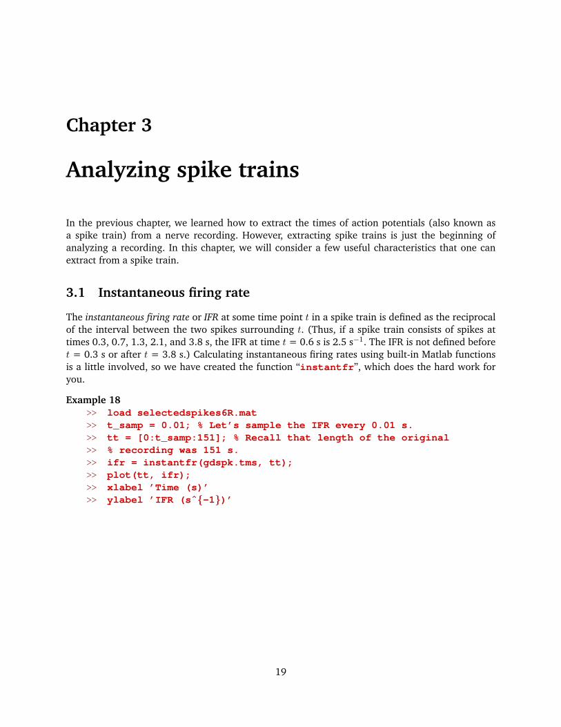
The instantaneous firing rate or IFR at some time point t in a spike train is defined as the reciprocalof the interval between the two spikes surrounding t. (Thus, if a spike train consists of spikes attimes 0.3, 0.7, 1.3, 2.1, and 3.8 s, the IFR at time t = 0.6 s is 2.5 s−1. The IFR is not defined beforet = 0.3 s or after t = 3.8 s.) Calculating instantaneous firing rates using built-in Matlab functionsis a little involved, so we have created the function “instantfr”, which does the hard work foryou.

Example 18>> load selectedspikes6R.mat>> t_samp = 0.01; % Let’s sample the IFR every 0.01 s.>> tt = [0:t_samp:151]; % Recall that length of the original>> % recording was 151 s.>> ifr = instantfr(gdspk.tms, tt);>> plot(tt, ifr);>> xlabel ’Time (s)’>> ylabel ’IFR (sˆ{-1})’

19

(This example assumes that you saved the results of spike sorting as suggested at the end of chap-ter 2.)

Exercise 18What happens if you sample IFR at 0.1-s intervals or 1-s intervals? Do you still get a fairrepresentation of the data?

3.2 Smoothing the firing rate

In some neural codes, such as in the auditory system of owls, the timing of individual spikes isof great importance. In many other cases—and to our knowledge in all leech neurons—only therate of spikes in some time interval matters. One way to calculate this rate is to simply compute ahistogram of spikes in time bins of some reasonable size, e.g., 1 s:

>> hist(gdspk.tms, [0:1:151]);

This plots the results; if you want to store the results in a variable instead, you’d write:

>> [fr, t] = hist(gdspk.tms, [0:1:151]);

Then you could plot the results by typing “plot(t, fr)” or—to get a bar graph just like the oneproduced by the “hist” function—by typing “bar(t, fr)”.

A visually more pleasing result which also doesn’t suffer from the random effects of spikes fallingjust to the left or to the right of the edge between two bins can be obtained by sampling usingsmaller bins, and applying a low-pass filter.

20

Example 19>> t_samp = 0.01; % Sample in bins of 0.01 s.>> tau = 1; % Low-pass to τ = 1 s.>> [fr, tt] = hist(gdspk.tms, [0:t_samp:151]);>> [b, a] = butterlow1(t_samp / tau); % Prepare the filter.>> ffr = filtfilt(b, a, fr / t_samp); % Calculate smoothed FR.>> plot(tt, ffr);

(Note for the curious: “butterlow1(f_0/f_s)” prepares a first-order low-pass Butterworth fil-ter with cut-off frequency f0/fs, and “filtfilt” applies that filter twice, once in the forwarddirection, and once backwards. The net result is a second-order low-pass filter with zero phaseshift.)

Exercise 19Create a figure that contains both the IFR from example 18 (in blue) and the smoothedfiring rate from example 19 (in red). Zoom in on a burst. Do you understand the differ-ences between the two curves? Advanced: Why is it not a good idea to use the IFR asthe starting point for smoothing. (DAW is happy to discuss.)

Depending on your application, various different timescales can be used for the calculation of firingrates. In the example below, we use τ = 0.1 s, 1 s, 10 s, and 100 s.

Example 20 (Continued from example 19.)>> taus=[0.1 1.0 10 100];>> clf; hold on>> clr=’grbk’;>> for k=1:4>> [b, a]=butterlow1(t_samp / taus(k));>> ffr = filtfilt(b, a, fr / t_samp);>> plot(tt, ffr, clr(k));>> end>> legend(’\tau = 0.1 s’, ’\tau = 1.0 s’, ...

’\tau = 10 s’, ’\tau = 100 s’);

21

Exercise 20Can you add a line to the figure created in the above example that represents the av-erage firing rate? In calculating the average, does it matter (much) whether you firstapply a low pass filter? Why (not)?

3.3 Detecting and characterizing bursts

As should be obvious from any of the preceding graphs, cell DE-3 does not fire tonically. Rather, itfires bursts of many action potentials separated by several seconds without much activity. Under-standing these bursts could be key to understanding the neural code.

If you look back to the graph of the instantaneous firing rate produced by example 18, you noticethat the IFR is never less than 1 s−1 inside the bursts, and never more than that outside the bursts.Thus, we can detect bursts by looking for intervals of 1 s or more without spikes. we have createdthe function “burstinfo” to perform this detection and to extract some useful parameters abouteach burst. In the example below, just a few of these parameters are used; type “help burstinfo”to learn what else is available.

Example 21>> load selectedspikes6R.mat>> bi = burstinfo(gdspk.tms, 1.0, 151); % The last parameter ...

% specifies the length of the recording.>> clf; hold on>> plot(gdspk.tms, gdspk.amp / max(gdspk.amp), ’k.’);>> plot(bi.t_start, 1.1, ’r<’);1

>> plot(bi.t_end, 1.1, ’r>’);>> axis([0 151 0.7 1.2])>> xlabel ’Time (s)’

1Note for aficionados: The latest version of Matlab allows you to plot a scalar against a vector (as in“plot(bi.t_start, 1.1)”). It automatically turns “1.1” into a vector of the right length.

22

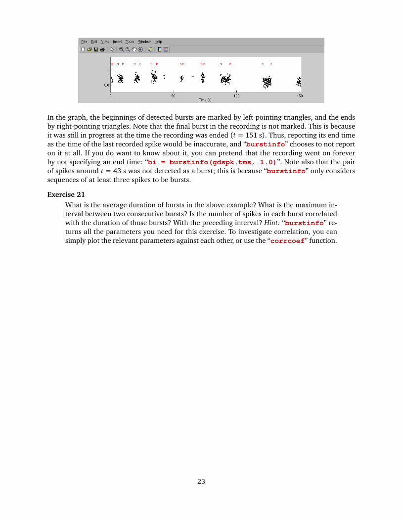
In the graph, the beginnings of detected bursts are marked by left-pointing triangles, and the endsby right-pointing triangles. Note that the final burst in the recording is not marked. This is becauseit was still in progress at the time the recording was ended (t = 151 s). Thus, reporting its end timeas the time of the last recorded spike would be inaccurate, and “burstinfo” chooses to not reporton it at all. If you do want to know about it, you can pretend that the recording went on foreverby not specifying an end time: “bi = burstinfo(gdspk.tms, 1.0)”. Note also that the pairof spikes around t = 43 s was not detected as a burst; this is because “burstinfo” only considerssequences of at least three spikes to be bursts.

Exercise 21What is the average duration of bursts in the above example? What is the maximum in-terval between two consecutive bursts? Is the number of spikes in each burst correlatedwith the duration of those bursts? With the preceding interval? Hint: “burstinfo” re-turns all the parameters you need for this exercise. To investigate correlation, you cansimply plot the relevant parameters against each other, or use the “corrcoef” function.

23

Intermezzo

Congratulations! You have covered all the ground needed to analyze the data from today’s labexercise. The remaining chapters of this tutorial introduce several other techniques that you mayfind useful for analyzing electrophysiological data, but they are not critical for today’s work. wesuggest you read them at your leisure.

We hope the whirlwind pace of chapters two and three hasn’t overwhelmed you. It is no problemat all if you have not understood all of the fine points. We just hope you will take home the lessonthat Matlab is a very flexible tool, and that you are now not afraid to further explore it on yourown. For those of you who still feel uncomfortable working with Matlab, that is okay as well; asyou have learned in the various demos, your pClamp software has built-in routines that can coversome of the basics of the analyses presented here (e.g., spike detection). DAW has used Matlab forover a decade now, and is still getting better at it, so please do not be discouraged if this tutorialfelt a little (or very) overwhelming; we covered a lot of material in a very short time. Do feel freeto come to us with any questions you may have, even if you’re not sure how to phrase them.

On a final note, although this tutorial has spoken exclusively about Matlab, we do not want toleave you with the impression that Matlab is the only game in town. In fact, there are several othersoftware packages that allow you to do this sort of analysis. We would like to mention three byname, because they are free and open-source software (unlike Matlab which costs money).

The first, “Octave,” is almost a drop-in replacement for Matlab, if you can live without Matlabs’spolished user interface and many of its toolboxes. Apart from that, Octave is so much like Matlabthat all of the examples from chapter one work just fine in Octave. The current version of Octave(http://www.gnu.org/software/octave) still misses a few functions so that “selectspike” doesn’trun, but I have created a special version (called “iselectspike”) that works on the Linux version ofOctave and can probably be made to work on the Mac and Windows versions. Let me know if youare interested in using this.

The second, “SciPy,” is also similar to Matlab in intent, but quite different in implementation: itis a collection of extensions to the Python language. SciPy is very much worth exploring, and notonly if your institute doesn’t subscribe to Matlab. A particularly nice way to use SciPy is from withinthe “Jupyter” system, which allows you to keep analysis notes right along with your code. A goodstarting point to learn about SciPy is http://scipy.org. Most Linux distributions have precompiledversions available, and Windows downloads are available through the web page. Jupyter is athttp://jupyter.org. If you like Python, you may well love SciPy. Otherwise, Matlab/Octave may beeasier to learn.

Finally, there is “R,” which is targeted specifically at statistics. It contains built-in support forany statistical test you are ever likely to encounter, good graphics support, and excellent documen-tation, but its handling of large data sets and general programming support is not quite as good asMatlab, Octave, or SciPy. R may be found at http://www.r-project.org/, and as part of many Linuxdistributions. (For Ubuntu, e.g., the package to install is called “r-base.”)

Good luck analyzing your data!

24

Chapter 4

Detecting intracellular spikes

Note: We do not expect you to get to this chapter before moving on to today’s lab work. You can workon it later as your schedule permits.

In the previous two chapters, we analyzed extracellularly recorded spikes. What if you have anintracellular recording? After the initial step of detection, analyzing intracellularly recorded spiketrains is no different from extracellularly recorded ones: in either case, one works with a seriesof timestamps. However, the process of detecting intracellular spikes is quite different from theone for extracellular spikes, because intracellular spikes have a different shape than extracellularspikes, and intracellular recordings are susceptible to different sources of noise. In this chapter, wewill discuss how to handle these.

For your reference, I have stored all of the following code in a script file called “intracel.m”.

Example 22>> load intracel.mat

>> figure(1); clf>> subplot(2, 1, 1);>> plot(tt, ii);>> xlabel ’Time (s)’>> ylabel ’Current (nA)’

>> subplot(2, 1, 2);>> plot(tt, vv);>> xlabel ’Time (s)’>> ylabel ’Voltage (mV)’

Exercise 22I surreptitiously introduced the function “subplot” in the above example. As yousee, this splits a figure window so that it can contain multiple graphs. Type “helpsubplot” to learn more, and create a 2x2 layout of the raster plots and firing rateplots of the left and right DP1 nerve recordings in the data set we used in the previoustwo chapters. Save your code in a “.m” file for future reference.

The data in example 22 are from a recording by Krista Todd. The top trace shows injected current,the bottom trace recorded voltage from a DE-3 cell in a preparation where the ganglion was left

25

attached to a portion of body wall so that muscle actions could be observed. Looking at the graphs,you will notice that the voltage trace is badly polluted by at least two artefacts: (1) bridge balancewas incomplete, resulting in a jump near the start and end of the stimulus, and (2) during the be-ginning of the stimulus, the baseline voltage drifted considerably (due to motion artefacts). Pleasenote that these problems should not be blamed on Krista; intracellular recording from this kind ofpreparation is quite a tour-de-force. Still, we need to remove them in order to reveal the actionpotentials.

4.1 Removing the voltage steps caused by the bridge imbalance

Our first step will be to remove the big voltage steps at the beginning and end of the stimulus. Todo this semi-automatically, the following Matlab code detects the transients in the current trace andsubtracts the corresponding jumps from the voltage trace.

Example 23>> L=length(vv);>> DI=4;>> yy=vv;>> badidx=find([nan ...

abs(diff(ii))]>.1);>> for k=1:length(badidx)

i0=max(badidx(k)-DI, 1);i1=min(badidx(k)+DI, L);v0 = yy(i0);v1 = yy(i1);yy(i1:end)=yy(i1:end) ...+ v0-v1;

yy(i0+1:i1-1)=v0;end

>> figure(2); clf>> plot(tt, yy);>> xlabel ’Time (s)’>> ylabel ’Voltage (mV)’

Note for the curious: we measured the recorded voltage DI = 4 samples before and after the step,and subtracted the difference.

Exercise 23Why did I write “max(badidx(k)-DI, 1)” in the example? Could I simply have writ-ten “badidxk-DI”? (What if one of the current steps was very close to the beginningof the recording?)

4.2 Removing the motion-induced drift

Looking at the graph in example 23, it is obvious that this procedure only solved part of the prob-lems, so let’s keep working. To remove the baseline drift induced by motion, we simply filter awayany signal with frequencies below 50 Hz:

26

Example 24>> dt_s = mean(diff(tt));>> f0_hz = 1/dt_s;>> fcut_hz = 50;>> [b, a]=butterhigh1...

(fcut_hz/f0_hz);>> zz=filtfilt(b, a, yy);

>> figure(3); clf>> plot(tt, zz);>> xlabel ’Time (s)’>> ylabel ’Voltage (mV)’

Exercise 24Experiment with different values of the cutoff frequency in the above example. Might25 Hz or 100 Hz be better than 50 Hz? How would you judge?

4.3 Removing the 60 Hz pickup

The zoom on the right below example 24 shows that action potentials are now clearly distinguish-able, but a fair bit of 60 Hz pickup, previously obscured by the larger artefacts, has also becomeevident. The most effective way I know to remove such pickup, is to use a template filter. The detailsof the method are beyond the present tutorial; if you are interested, feel free to look at the sourceof “templatefilter”, or to ask me for an explanation.

Example 25>> ww = templatefilter(zz, ...

f0_hz/60, 200/f0_hz,50);

>> figure(4); clf>> plot(tt, ww);>> xlabel ’Time (s)’>> ylabel ’Voltage (mV)’>> axis([3 4 -1 2])

Exercise 25 (For die-hards)Experiment with the parameters of “templatefilter”.

After removing all these artefacts, the trace looks reasonably clean; time to detect action potentials.

27

4.4 Detecting the actual action potentials

If you zoom around in the trace, you will notice that the amplitude of action potentials is quitevariable, especially during the stimulus. In cases like this, it may take a bit of trial and error to findthe best threshold. We can use the same basic technique as for extracellular spikes, but the firingrate in this example is so high that we must use a shorter window than before to estimate the RMSnoise, and also a lower initial threshold:

Example 26>> spk=detectspike(ww, tt, 2,

2);>> gdspk=selectspike(spk);

The “selectspike” window after dragging thethreshold lines to my best estimate.

>> figure(5); clf>> plot(tt, ww);>> hold on>> plot(spk.tms, spk.amp, ’k.’);>> plot(gdspk.tms, gdspk.amp,

’r.’);>> xlabel ’Time (s)’>> ylabel ’Voltage (mV)’

Exercise 26Do you agree with where I drew the threshold line in the above example? Can you dobetter?

4.5 Conclusion

If you did the last exercise, you will have realized that, in cases like this where the signal-to-noiseratio is very low, setting a threshold will always be somewhat arbitrary. Still, this method probablyyields a reasonably good estimate of the firing rate. Of course, if you are recording from a Retziusor sensory cell—with much larger action potentials—your signal-to-noise ratio will be a lot better,and your confidence in spike detection will be correspondingly greater.

28

Chapter 5

Analysis of multiple spike trains

If you have simultaneously recorded data from multiple intracellular or extracellular electrodes,you can of course use the techniques from the previous chapters to analyze the recordings sep-arately. Frequently, however, much can be learned from the relationship between two recordingchannels. In this chapter, we will consider the example of a simultaneous intracellular and extracel-lular recording from the same neuron. In particular, we shall be concerned with the delays betweenrecorded spikes. For the examples below, you may either use your own data, or the test data setprovided.

5.1 Loading the raw data and extracting spike times

The obvious first step is to load the data into Matlab:

>> [vlt, tms] = loadephys(’intraextra.xml’);

(These data were stored in a special file format defined by acquisition software created in my lab,but you don’t need to worry about the details: “loadephys” knows how to load the relevant data.)

Let’s take a look at what we loaded:

>> whosName Size Bytes Class

tms 110000x1 880000 double arrayvlt 110000x6 5280000 double array

Unlike in the example in Chapter 2, there are only three channels of interest here: Intracellularvoltage is stored in channel 2, intracellular current in channel 4, and extracellular voltage in chan-nel 6. (Data from a second extracellular electrode is in channel 5, but those data are not of interesthere.)Scale factors have not been properly preserved (because of a bug in the software I used to recordthese data), so let’s avoid confusion by giving better names to the various signals:

>> Vint mV = vlt(:,2);>> Iint nA = vlt(:,4)/10;>> Vext uV = vlt(:,6)/10;

With that, let’s start by looking at the various signals. We’ll plot them in three “subplots,” and use aclever Matlab trick to allow zooming into all three at the same time:

29

>> figure(1); clf>> subplot(3, 1, 1); plot(tms, Vint mV, ’b’);>> subplot(3, 1, 2); plot(tms, Iint nA, ’r’);>> subplot(3, 1, 3); plot(tms, Vext uV, ’k’);>> linkaxes(get(gcf, ’children’), ’x’);

(If you are using an older version of Matlab at home, you won’t have the “linkaxes” functionavailable, so you might be better off plotting everything in one plot.)

The results of the previous plot commands (left), and after labeling the axes and zooming in (right).

In the top panel, the “rabbit ears” resulting from the current steps are clearly visible, as are theevoked action potentials. In the bottom panel, spikes from several different cells can be seen, andit is hard to tell which ones belong to the neuron with the intracellular electrode in it. Perhaps itmight help to overlay the intracellular and extracellular traces?

>> figure(2); clf; hold on;>> plot(tms, Vint mV, ’r’);>> plot(tms, Vext uV/3+20, ’k’);>> xlabel ’Time (s)’>> ylabel ’V int (mV)’>> axis([.95 1.5 -100 60]);

30

(I hand-drew those green annotations.) Now, we can clearly see that extracellular spikes of a specificsize tend to follow intracellular spikes.

Exercise 27 (Not Matlab-related.)What do you think happened during the second stimulus?Hint: What extracellular event occurred just before the expected spike?

We could now proceed to extract the extracellular spikes as in Chapter 2, and to extract the in-tracellular spikes as in Chapter 4, but picking out the right extracellular spikes might be difficultbecause of the presence of other spikes of similar amplitude. Let’s therefore try something else.

Detecting spikes in very clean intracellular recordings like this one should be easy, and it is. I’vewritten a convenient Matlab function that let’s you pick them out:

>> intspk = selspktrace(Vint mV, tms);

The “selspktrace” window after zooming and dragging the limit lines to appropriate locations.

Exercise 28 (For hardy souls.)In this case, the rabbit ears are easily distinguished from the action potentials by am-plitude. If the rabbit ears in your recording are taller, their widths should still be quiteshort, and thus distinctly not action potential–like. Write a Matlab function to exploitthis characteristic and toss out the rabbit ears from the list of spikes in “intspk”.

Now we know when each of the intracellular spikes happened. Thus, we could look at the extracel-lular trace right around these events. The most direct way to do that might be this:

>> figure(1); clf; hold on>> N = length(intspk.tms);>> clr = jet(N);>> for k=1:N

idx=find(tms==intspk.tms(k));if idx>200 & idx<length(tms)-200

plot(tms(idx-200:idx+200)-tms(idx), ...Vext uV(idx-200:idx+200), ’color’, clr(k,:));

endend

31

The result looks like this:

To take the tedium out of that, I’ve created a a function that automatically extracts data aroundevents. As a bonus, it also calculates the “event-triggered average”: the average of the data collectedaround each of the events. You use it like this:

>> [avg, dt, indiv] = trigavg(Vext uV, tms, intspk.tms);>> subplot(2, 1, 1); plot(dt, avg);>> subplot(2, 1, 2); plot(dt, indiv);

(I’ve labeled the axes, recolored the traces, andzoomed in a little before taking that screenshot.)

Exercise 29Can you overlay the average intracellular trace on the top panel of the above graph?

Based on the output of “trigavg”, calculating things like the average propagation delay is straight-forward:

>> [mx, idx] = min(avg);>> avgdelay = dt(idx)avgdelay =

5.9

32

Exercise 30 (Not Matlab-related).Why did I consider the time of the extracellular spike to be the time of its negativepeak?

Exercise 31How can you tell whether any intracellular events did not cause a corresponding extra-cellular spike? Could you encode your answer as a Matlab function that automaticallyfinds out which action potentials failed to propagate?

One rather elaborate solution to that last exercise are the functions “trigavgmax” and “trigavgfail”.Especially “trigavgmax” is more general and more ambitious in its scope than would be strictlynecessary for this application, but you may be interested to read the source code. Regardless, theywork like this:

>> [avg, dt, indiv] = trigavg(Vext uV, tms, intspk.tms);>> [mxx, dtt] = trigavgmax(-indiv, dt);>> failures = find(trigavgfail(mxx));

33

Chapter 6

Some notes on further analysis

This chapter contains some notes on further analyzing your data. It is not nearly as thorough asprevious chapters, but hopefully at least somewhat useful.

6.1 Measuring time constants

In this section, we will use Matlab to more accurately measure time constants than the standardmethod of eyeballing the delay until a signal has decayed to one third of its original size. Whilethat method is often good enough, greater accuracy is called for if you are going to publish data.Moreover, the method described here, which consists of fitting an exponential curve to the data,provides an example of the more general problem of function fitting, which you will encounter inmany other guises.

Let’s start by loading a small data set:

>> [dat, tms] = loadephys(’timecst.abf’);’>> figure(1); clf; subplot(2, 1, 1)>> plot(tms, dat(:, 1);>> subplot(2, 1, 2);>> plot(tms, dat(:,3);

The bottom trace shows the current applied to an RC circuit; the top trace shows the resultingvoltage. We are going to determine the time constant of each of the transitions. By zooming intothe graphs, it is easy to determine that the transitions occur at 0.12 s, 0.62 s, 1.12 s and 1.62 s.Alternatively, you can use Matlab to find the transitions:

34

>> [iup, idn] = schmitt(dat(:,3), -0.2, -0.4, 1);>> iup=iup(iup>1);>> ttrans = tms(sort([iup; idn]))’

ttrans =

[ 0.1160 0.6160 1.1160 1.6160 ]

(The function “schmitt” reports an upward transition at the beginning of the trace because theinitial voltage is above its threshold; the second line above drops this transition from further con-sideration.)

Let’s fit an exponential to the first transition:

>> t0 = ttrans(1)

t0 =

0.1160

>> idx = find(tms>t0+0.002 & tms<t0+0.40);>> [fit, yy] = physfit(’expc’, tms(idx), dat(idx,1));>> subplot(2, 1, 1); hold on; plot(tms(idx), yy1, ’r’);>> fit.p

ans =

1.0e+03 *3.5716 -0.0428 -0.0249

What do those numbers mean? Let’s ask Matlab!

>> fit.form

ans =

A*exp(B*x) + C

So, Matlab is telling us that this part of the trace is fit by

3571.6 e−42.8t − 24.9.

In other words, τ = 1/42.8 = 0.0233 s and the trace asymptotes to −24.9 mV. The red trace overlaidon the data is the fitted curve; evidently, the fit quality is pretty good.

35

Exercise 32Based on those numbers, can you calculate the values of R and C? Note that the currentinjected was:

>> mean(dat(idx, 3))

ans =

-0.5204

i.e., 0.52 nA.

Let’s step back for a moment, and consider what we just did. The main magic was the “physfit”call. This function is a general function fitter. It can fit straight lines, sinusoids, polynomials, expo-nentials, and several other predefined functional forms, as well as arbitrary user-defined functions.Beside returning the fit parameters (in “fit.p”), it also tells you the uncertainty in those parame-ters (in “fit.s”). If you tell it the uncertainty in your data, it will also report the quality of the fit.For instance, you could measure the noise inherent in your data:

>> noise = std(dat(tms<t0-0.05), 1)

noise =

0.0783

and feed that to “physfit”:

>> [fit, yy] = physfit(’expc’, tms(idx), dat(idx,1),noise);>> fit(2).chi2

ans =

1.0711

Since χ2 is close to one, we conclude that the fit is indeed very good. (If you call “physfit” in thisway, “fit(1)” returns a fit of the data that disregards the uncertainties, and “fit(2)” returns afit that uses the uncertainties.)

Exercise 33Fit curves to the other transitions. Do the numbers agree? Hint: The elegant solutionuses a “for” loop.

Obviously, we have only scratched the surface of what “physfit” can do, but hopefully you nowhave a basis for further explorations on your own.

36