an electrical resistivity survey in the avra...
TRANSCRIPT

An electrical resistivity survey in theAvra Valley, Pima County, Arizona
Item Type text; Thesis-Reproduction (electronic)
Authors Qahwash, Abdellatif Ahmad, 1940-
Publisher The University of Arizona.
Rights Copyright © is held by the author. Digital access to this materialis made possible by the University Libraries, University of Arizona.Further transmission, reproduction or presentation (such aspublic display or performance) of protected items is prohibitedexcept with permission of the author.
Download date 11/06/2018 10:29:18
Link to Item http://hdl.handle.net/10150/566433

AN ELECTRICAL RESISTIVITY SURVEY IN THE AVRA VALLEY,
PIMA COUNTY, ARIZONA
by
Abdellatif Ahmad Qahwash
A Thesis Submitted-to the Faculty of the
DEPARTMENT OF MINING AND GEOLOGICAL ENGINEERING
In Partial Fulfillment of the Requirements For the Degree of
MASTER OF SCIENCEWITH A MAJOR IN GEOLOGICAL ENGINEERING
In the Graduate College
THE UNIVERSITY OF ARIZONA
1 9 7 2
STATEMENT BY AUTHOR
This thesis has been submitted in partial fulfillment of requirements for an advanced degree at The University of Arizona and is deposited in the University Library to be made available to borrowers under rules of the Library.
Brief quotations from this thesis are allowable without special permission, provided that accurate acknowledgment of source is made. Requests for permission for extended quotation from or reproduction of this manuscript in whole or in part may be granted by the head of the major department or the Dean of the Graduate College when in his judgment the proposed use of the material is in the interests of scholarship. In all other instances, however, permission must be obtained from the author.
SIGNED: -A A-
APPROVAL BY THESIS DIRECTOR
This thesis has been approved on the date shown below:
W. C. L # yProfessor of Mining andGeological Engineering
Date

ACKNOIVLEDGNENTS
The author wishes to express his sincere appreciation and
gratitude to Dr. Willard C. Lacy for his suggestions and direction
during the formulation of this thesis.
The author is greatly indebted to Dr. John S. Sumner for his
critical review of this thesis.

TABLE OF CONTENTS
Page
LIST OF ILLUSTRATIONS ...................... . . . . . . vi
LIST OF TABLES ......................................... viii
ABSTRACT......... ix
1. INTRODUCTION.......................... 1
Location....................................... 2Geology ........................................... 4
Mountain Area................................... 4Pediment Area. .................................. 9Alluvial Area................................... 9
2. THEORETICAL CONSIDERATIONS OF GEOELECTRICAL RESISTIVITYMEASUREMENTS ........................................... 11
Resistivity...................."................ . . 11Theory of Current Flow in a Homogeneous Earth......... 12Concept of Apparent Resistivity...................... 14The Formula of the Earth's Electrical Resistivity
Using Wenner Electrode Arrangement............... 15Electrical Anisotropy and Inhomogeneity............... 16Electrical Resistivity of R o c k s .................. . 17
3. FIELD SURVEY....................................... . . 20
Introduction....................................... 20Instruments............. 20. Field Techniques................................... 22Analysis of the Vertical Sounding Field Curves....... 23Results and Interpretation of the Vertical Electrical
Sounding Field Curves............................ 25The VES 1 Curve..................... 27The VES 2 Curve.................................. 32The VES 3 Curve.................................. 32The VES 4 Curve.................................. 37
4. HORIZONTAL PROFILING............. 41
Introduction ....................................... 41Analysis of the Profiling Data ................. . . . 48
iv

V
TABLE OF CONTENTS- - Continued
Page
5. CONCLUSIONS.................. ...........\ . 64
LIST OF REFERENCES .............................. . 66

LIST OF ILLUSTRATIONS
Figure Page
1. Index map of Avra Valley showing location of areaof study......................................... . 3
2. A general configuration of point electrodes over a homogeneous and isotropic e a r t h .......................... 14
3. Wenner electrode array for apparent resistivity measurements ....... . . ..................... . 15
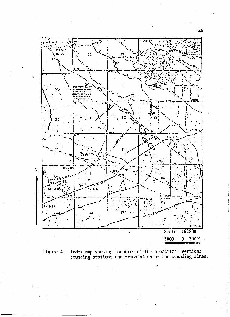
4. Index map showing location of the electrical verticalsounding stations and orientation of the sounding lines. . 26
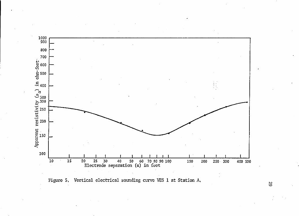
5. Vertical electrical sounding curve VES 1 at Station A . . 29
6. Vertical electrical sounding curve VES 2 at Station B . . 34
7. Vertical electrical sounding curve VES 3 at Station C . . 36
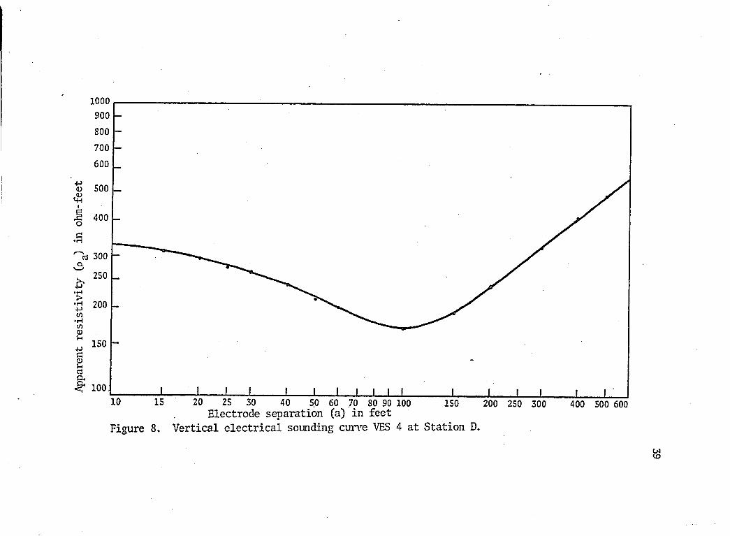
8. Vertical electrical sounding curve VES 4 at Station D . . 39
9. Theoretical horizontal resistivity profiles across verticalperfectly insulating and conducting planes with Wenner configuration....................................... 44
10. Theoretical horizontal resistivity profile across a vertical fault with Wenner configuration; traverses takenat different angles to the f a u l t ..................... 46
11. Theoretical horizontal resistivity profile with Wennerconfiguration along traverse perpendicular to strike of fault dipping 4 5 ° ................................... 47
12. Index map showing location of the electrical horizontal profiling stations and orientation of the profiling lines. 52
13. Horizontal resistivity profile No. 1 with two dimensionalmodel used for interpretation.......................... 53
14. Horizontal resistivity profile No. 2 with two dimensionalmodel used for interpretation. ......................... 54
vi

vnLIST OF ILLUSTRATIONS--Continued
Figure Page
15. Horizontal resistivity profile No. 3 with two dimensionalmodel used for interpretation......................... 55
16. Comparison of theoretical field and observed field horizontal resistivity profiles: (a) observed field curveNo. 1 (b) observed field curve No. 2 (c) Theoreticalfield plot over a fault.............................. 60
17. Comparison of theoretical field and observed fieldhorizontal resistivity profiles: (a) observed field curveNo. 3 (b) theoretical field plot over a fault dipping 45°. 61

LIST OF TABLES
Table Page
1. Calculated apparent resistivities at Station A ......... 28
2. Interpretation of the VES 1 c u r v e .................... 30
3. Results of a drilling log at well (D-14-12) 33bdb....... 31
4. Calculated apparent resistivities at Station B .......... 33
5. Calculated apparent resistivities at Station C ......... 35
6. Interpretation of the VES 3 c u r v e .................... 37
7. Calculated apparent resistivities at Station D .......... 38
8. First interpretation of the VES 4 curve................. 40
9. Second interpretation of the VES 4 curve.............. 40
10. Calculated apparent resistivities along traverse No. 1 . . 49
11. Calculated apparent resistivities along traverse No. 2 . . 50
12. Calculated apparent resistivities along traverse No. 3 . . 51
viii

ABSTRACT
An electrical resistivity survey using the Wenner electrode
configuration was made in the Avra Valley, Pima County, Arizona.
Equipment used in the field work consisted of a Burr-Brown
induced polarization receiver, transmitter, and a generator. All
measurements were made at a frequency of 3 cps.
The field work was divided into two main parts:
1. Measurement and study of the variations in resis
tivity with depth, and
2. Detection of subsurface structural discontinuities
by a horizontal resistivity profiling survey.
The results of the vertical sounding profiles were interpreted
by the standard curve matching method, using the Mooney, and Wetzel
master curves. The sounding data were used to evaluate the thicknesses
and resistivities of the subsurface earth materials.
The horizontal profiling field curves were compared with the
oretical horizontal resistivity profiles computed from theoretical
apparent resistivity formulas derived through the application of
image theory.
The probable presence of a subsurface steep fault was determined
from the analysis of the horizontal profiling field curves. The cal
culated apparent resistivity values showed the most rapid changes when
the potential electrodes started to cross the subsurface scarp. This
ix

X
subsurface structural discontinuity may put some limitations upon the
selection of sites for mineral exploration or other engineering pro
jects.
CHAPTER 1
INTRODUCTION
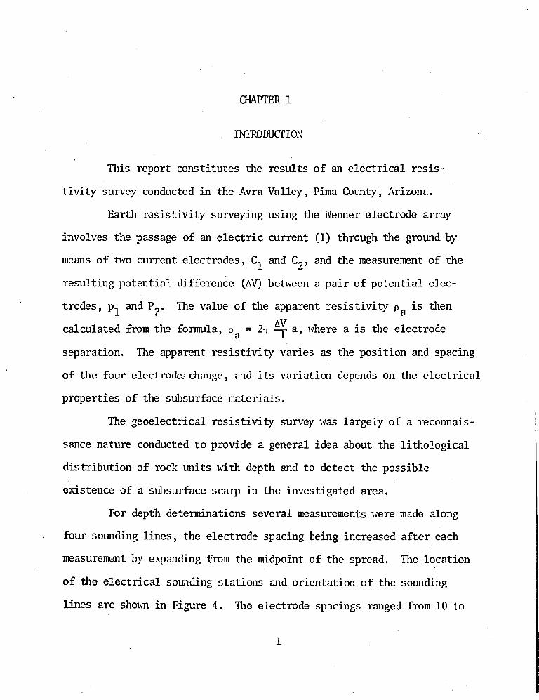
This report constitutes the results of an electrical resis
tivity survey conducted in the Avra Valley, Pima County, Arizona.
Earth resistivity surveying using the Wenner electrode array
involves the passage of an electric current (I) through the ground by
means of two current electrodes, C^ and C2, and the measurement of the resulting potential difference (AV) between a pair of potential elec
trodes, p^ and ?2 ' The value of the apparent resistivity pa is then
calculated from the formula, p = 2tt ^ a, where a is the electrode
separation. The apparent resistivity varies as the position and spacing
of the four electrodes change, and its variation depends on the electrical
properties of the subsurface materials.
The geoelectrical resistivity survey was largely of a reconnais
sance nature conducted to provide a general idea about the lithological
distribution of rock units with depth and to detect the possible
existence of a subsurface scarp in the investigated area.
For depth deteimnations several measurements 'were made along
four sounding lines, the electrode spacing being increased after each
measurement by expanding from the midpoint of the spread. The location
of the electrical sounding stations and orientation of the sounding
lines are shown in Figure 4. The electrode spacings ranged from 10 to
1

2600 feet. The vertical sounding data were plotted on a double loga
rithmic paper of the type Keuffel and Esser 358-110L (2x2 cycle),
using electrode spacing in feet as abscissas and calculated apparent
resistivity in ohm-feet as ordinates.
Interpretation of the sounding data was made by comparing the
field curves with theoretical curves conputed for horizontally strati
fied homogeneous layers (Mooney and Wetzel 1956). A match of a field
curve with a master curve is considered as a match of their respective
properties.
Three horizontal profiles were made with a constant electrode
spacing of "a" equal to 800 feet and the successive stations were spaced
at intervals of 800 feet. The graphs of these horizontal profiles,
shown in Figures 13 to 15, were plotted with the apparent resistivity
in ohm-feet as ordinates and with distance divided into stations at 800
feet intervals as abscissas.
Location
Avra Valley is about 15 miles west of Tucson, Pima County,
Arizona (Figure 1). The area of study is bordered on the east-northeast
by the Tucson Mountains, on the south-southeast by State Highway 86
and Snyder Hill, and on the far west by the Roskruge Mountains. The
general trend of Avra Valley is from south to north where it finally
joins the valley of the Santa Cruz River. The valley is drained by
intermittent streams that carry water only during the rainy periods.

3
AvraValley
Tucson \ Mountains
Tucson
SnyderHill
Del Bac HillsThree Points
AltarValley
Sierrita Mbuntains
10 MilesArizona
Scale:Tucson 575,000
Figure 1. Index map of Avra Valley showing location of area of study.

Brawley Wash is the principal drainage feature in Avra Valley. The floor
of the valley is filled with clay, gravel and sand.
Geology
The area starting from the Tucson Mountains to the central part
of Avra Valley can be classified into:
1. Mountain area,
2. Pediment area, and
3. Upper and lower alluvial area.
Mountain Area
Geologic investigations of the Tucson Mountains have been car
ried out by a number of geologists. Brown (1939) made a detailed study
of the geology of the Tucson Mountains. Britt (1955) reported on the
stratigraphy of the TYrin Peaks area and Bennett (1957) studied the geol- .
ogy of the Sedimentary Hills. Whitney (1957) studied the geology of an
area in the east-central part of the range. Kinnison (1958) described
the geology of the Tucson Mountains south of Ajo Road, and Colby (1958)
reported on the geology of the Red Hills and Brown Mountain. Bike man
and Damon (1966) divided the range into a dip slope on the east, a high
escarpment on the west and a large plutonic mass in the west-central part.
Mayo (1968) gave a summary of geologic investigations in the Tucson
Mountains from 1905 to 1968.
Rocks of each geologic era are found in the Tucson Mountains.
Precambrian Pinal Schist and Paleozoic rocks are found at Twin Peaks,
in the extreme north end of the Tucson Mountains. Britt (1955)
4

5
measured 700 feet of Precambrian Pinal Schist and about 2,500 feet of
Paleozoic sedimentary rocks. The Paleozoic rocks consist mostly of
limestones except for the Middle Cambrian Bolsa Quartzite which uncon-
formably overlies the Precambrian Pinal Schist.
Permian Sedimentary rocks occur at Snyder Hill. They consist
of dark gray to black limestone and dolomite with subordinate units
of quartzite. Bryant (1955) assigns the lower limestone to the upper
Concha and the dolomite to the upper Rain Valley formation.
Brown (1939) recognized three Mesozoic rock units which are, '
in ascending order, the Cretaceous volcanic rocks, the Recreation Red
Beds, and the Amole Arkose. The Cretaceous volcanic rocks unit may
reach a thickness of 2,000 to 5,000 feet, and it consists mostly of
andesite with some rhyolites. The Recreation Red Beds unit crops out
mostly in the Red Hills, the type locality, and on Brown Mountain.
Whitney (1957) mentions the presence of red beds on the northeast slope
of the Tucson Mountains. Similar red beds are also found in the central
part of the Amole foimation in the Golden Gate Mountain area. Colby
(1958) divides the Recreation Red Beds into three members, the sandstone-
silts tone member, the volcanic conglomerate member, and the tuff member.
The Recreation Red Beds appear to be Lower^Cretaceous in age
(Colby 1958) since they underlie the Amole group. Damon (1967) ob
tained a potassium-argon date of 150 million years for andesite por
phyry that has intruded the Recreation Red Beds. This indicates that
the minimum age of this rock unit is . Jurassic.

6
The sediments which overlie the Recreation Red Beds are called
the Amole Arkose Formation (Brown 1939; Kinnison 1958). Kinnison
(1958) proposed that the Amole Arkose be renamed the Amole group since
the arkose is only one of the many rock types that are present in this
formation. The Amole group crops out mostly in the Sedimentary Hills
and in the Amole Mining District. Bennett (1957) divided the Amole
Formation in the Sedimentary Hills into a northern argillitic unit and
a southern limey unit, separated by a southwest-dipping thrust fault.
The northern argillitic unit has been intruded by quartz monzonite and
granite porphyry. Davenport (1963) indicates the presence of another
parallel thrust zone concealed by alluvium to the southwest of the
thrust fault mapped by Bennett.
Kinnison (1958) established a new formation, the Tucson Mountain
Chaos. It consists of large fragments of all of the pre-Laramide rocks
in a disoriented arrangement. Its stratigraphic position is above the
steeply dipping rocks of pre-Laramide age and below the Tertiary Cat
Mountain Rhyolite. The Tucson Mountain Chaos is exposed on the pedi
ment and in the low escarpment south of the Ajo Road. It is also ex
posed at scattered points in the area between the Cat Mountain and
Gates Pass. In the central part of the eastern dip side of the range,
a large area is composed of the Tucson Mountain Chaos. The chaos has
no exposures in the northern part of the range and in its place below
the Tertiary volcanic rocks are dark colored andesitic rocks. Kinnison
(1958) assumed that the Tucson Mountain Chaos is a sedimentary deposit
resulting from combined fault action and landslide. Bikerman (1963)

7
suggested that the Chaos is a pyroclastic flow breccia that represents
an initial phase of the volcanic activity which gave rise to the Cat
Mountain Rhyolite and terminated with the emplacement of the spherulitic
rhyolite. Mayo (1963) considered fluidization as a probable factor in
the development of the Tucson Mountain Chaos.
Above the Chaos lies a series of Tertiary volcanic rocks
which include, among others, the Cat Mountain Rhyolite, the Safford
Tuff, and the Shorts Ranch Andesites. The Cat Mountain Rhyolite
covers a large portion of the western escarpment of the range.
Bikerman (1962) described the lower light-colored Cat Mountain Rhyolite
as non-welded tuff and the upper dark-colored unit as welded tuff.
Mayo (1963) described this unit as ignimbrite consisting of ash flows
on the top and laccolithic masses below. The Short Ranch Andesite is
the uppermost unit of the Tertiary volcanic rocks. It is exposed on
the eastern side of the range north of the Ajo Road. At Twin Hills,
it overlies the Safford fo mat ion and Ivy May Andesite with angular
unconformity (Kinnison 1958). Elsewhere, it may conformably overlie
the Safford formation.
Several igneous rocks, with a wide variety of textures and com
positions, have intruded the Tertiary and older rocks. The Amole
Quartz Monzonite and the Amole Granite, which are contained in a com
posite stock that lies about three miles north of Red Hills, are the
major intrusive rocks in the Tucson Mountains.

8
Basalt flows dated as Tertiary-Quaternary are present at "A"
Mountain and at Tumamoc Hill. The basalt flows overlie unconformably
the Tertiary volcanic rocks.
Several theories have been advanced to account for the funda
mental structural elements in the Tucson Mountains. Brown (1939) con*-
sidered the large thrust fault and the tilted blocks as typical
structures of the range. He assumed that an extensive imbricate thrust
sheet advanced from the southwest across the present site of the moun
tains during Late Cretaceous time. Erosion reduced the thrust sheet
to remnants. Later investigations indicate that two structural events
dominate the Tucson Mountains, the Laramide Orogeny (Upper Cretaceous-
Paleocene) and the Basin-Range Orogeny (Upper Oligocene-Miocene).
The dominant elements of the Laramide Orogeny are broad
folding and intense deformation followed by block faulting and tilting.
The Cretaceous and older rocks-were intensely folded into asymmetrical
synclinorium with local thrust faulting during the Laramide Orogeny.
After the intense deformation, a period of extensive erosion planed
the Cretaceous and older rocks to a gentle relief surface which
Kinnison (1958) called the Tucson Surface.
The Tertiary volcanic rocks dip gently to the east direction
and they rest with angular unconformity on the Tucson Surface of the
older rocks. To the south of Ajo Road, the Tertiary rocks have been
complexly faulted by high angle faults and they exhibit folded struc
tures and variable directions of dip. Tiro sets of high angle faults
are found in the Tertiary rocks; most of them probably are normal

9
faults. One set strikes north-northeast and the other set strikes
west-northwest. Brown (1939) noted that the north-northeast faults
are nearly always downthrown to the south. This is not true in the
Saginaw area, where Kinnison (1958) noted the occurrence of many re
verse relationships.
During the second orogeny, the entire range is probably
bounded by basin-range block faults type and has been eroded with the
development of a widespread pediment. Such basin-range faults are
responsible for the present mountain-valley pattern.
Pediment Area
From the mountain bases a gently sloping bedrock surface,
covered with a thin layer of gravel and rock debris, extends downward
to the valley land. This bedrock slope, from which the steep mountains
rise abruptly, has been termed a mountain pediment. Bryan (1925) de
fined the pediment as a plain of combined erosion and transportation
at the foot of a desert mountain range.
Alluvial Area
The alluvium in Avra Valley consists of permeable lenses of
sand and gravel interbedded with clay and silt (White, Matlock, and
Schwalen 1966). The alluvium extends to depths as great as 2,000 feet
along the central part of the valley, but its thickness is considerably
less than 300 feet along the mountain fronts.
10
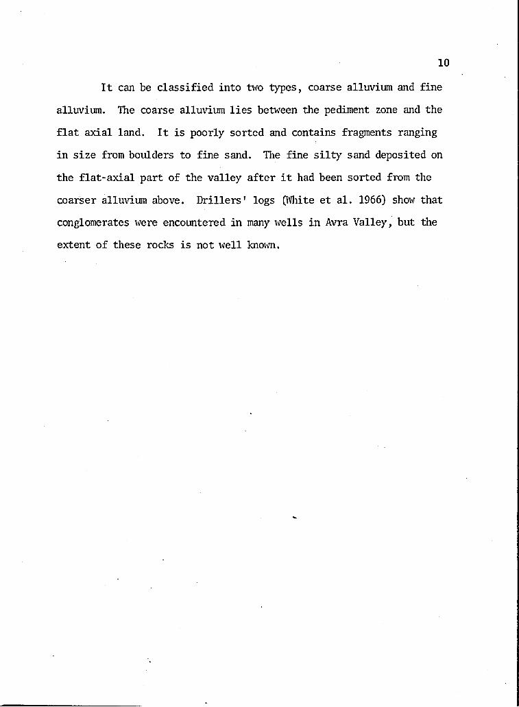
It can be classified into two types, coarse alluvium and fine
alluvium. The coarse alluvium lies between the pediment zone and the
flat axial land. It is poorly sorted and contains fragments ranging
in size from boulders to fine sand. The fine silty sand deposited on
the flat-axial part of the valley after it had been sorted from the
coarser alluvium above. Drillers' logs (White et al. 1966) show that
conglomerates were encountered in many wells in Avra Valley, but the
extent of these rocks is not well known.

CHAPTER 2
THEORETICAL CONSIDERATIONS OF GEOELECTRICAL RESISTIVITY MEASUREMENTS
Before going into the'details of the field work, it is essential
to consider the theoretical aspects of the earth resistivity measure
ments .
Resistivity
Electrical resistivity is a property of all earth materials, in
the same sense that density, magnetic susceptibility and elasticity are
properties of the rock masses.
Geoelectrical resistivity is defined as a measure of the resis
tance of a cylinder of rock sample, having for height the unit of length
and for cross-section the unit of area, to the flow of an electric
current through it.
Mathematically, this can be expressed as
R -
where R is the resistance of the rock sample
P is the resistivity
L is the length of the rock sample
A is the cross-sectional area.
AsR _ Voltage VK Current I
11

12
then
Materials such as quartz and dry wood are poor conductors and
have a high resistivity; other materials such as saltwater and copper
ar6 good conductors and have low resistivity.
Theory of Current Flow in a Homogeneous Earth
In geoelectrical resistivity measurements the current is
usually sent beneath the earth’s surface by means of two electrodes,
which can be mathematically treated as a point sources of equal and
opposite strength.
A point-source of strength I is defined as a point at which
electricity is generated at constant rate of I amperes. If we consider
a point-source of strength I on the surface of an infinite homogeneous
and isotropic ground of resistivity p and it is surrounded by a hemi
spherical surface of arbitrary radius R with its center at the point
source; then the current density J at any point on the surface of the
hemisphere is given by
To obtain the potential at any point with a distance r from
the point-source, we can use Ohm's Law in its differential form,
namely.
- Pj

13
by. integration
dv _ -pi^ ' 2,R2
dv = p ̂ 7 dr 2irRZ
V ~ " ^ R + C ‘
As the potential V is taken to be zero at a very large distance from the
point-source, the integration constant C = 0. Therefore,
2nR
where V is the electrical potential at a point on the surface of
a homogeneous earth
r is the distance from the point to the source of strength I
p is the true resistivity of a homogeneous earth.
From equation [1] an expression for the resistivity of the ground
can be derived when two current electrodes are used. So, if we con
sider an electric current of strength I introduced into a homogeneous
and isotropic earth by means of two electrodes and (Figure 2),
then the potential difference, AV, which will be observed between the
two other electrodes, p^ andP2 is defined as:
VPi - Vp2Using equation [1]:
AV = K [2]

14
where k, the configuration factor, is given by
Equation [2] can be solved for the resistivity
le ts]
where k", the geometrical factor, is equal to -=£■ .
Figure 2. A general configuration of point electrodes over a homogeneous and isotropic earth.
Concept of Apparent Resistivity
Equation [3] is applied only to a homogeneous ground. When the
earth is not homogeneous, as it is actually in nature, then the calcu
lated value of resistivity is called the "apparent" resistivity, desig
nated as pa-
The apparent resistivity, pa, of a geologic formation may be de
fined as the resistivity of an equivalent homogeneous and isotropic
medium in which the measured potential difference is equal to that for
the given inhomogeneous medium. This definition indicates that the value
of the apparent resistivity provides a measure of the deviation from a
homogeneous and isotropic medium.

15The Formula of the Earth's Electrical Resistivity Using Wenner Electrode Arrangement
The Wenner electrode arrangement shown in Figure 3 was used in
the geoelectrical resistivity field work.
Figure" 3. Wenner electrode array for apparent resistivity measurements.
C1 and 0-2 are the current electrodes, p^ and P2 are thepotential electrodes. The four electrodes are placed in line at equal distances apart on the surface of the earth.
For this array the configuration factor, k, is equal to ~ . Therefore
equation [2] can be written as
pa = 2n f a > [4]
where pa is the "apparent" resistivity of the earth, in ohm-feet,
a is the electrode separation in feet,
AV is the potential difference between p^aand p^ in volts,
I is the current flowing through the two current electrodes,
in amperes.

16
Electrical Anisotropy and Inhomogeneity
In theory, the medium under consideration is generally assumed
to be homogeneous and isotropic. This is not often encountered in
practice. It is well known that the conductivity of stratified rocks
is not the same in all directions; it is a maximum in the direction of
stratification, and a minimum in the direction perpendicular to strati
fication.
Fractures in rocks commonly follow the strike. Along these
fractures, when they are saturated with water, the electric current
travels with the greatest facility.
Stratified and fractured rocks, therefore, do not have the
same resistivity in all directions; they are called anisotropic
materials.
For each anisotropic material an electrical coefficient of
anisotropy y and an average resistivity pm are defined as
r -BPL
where is the longitudinal resistivity
Pj. is the transverse resistivity.

17
Electrical Resistivity of Rocks
Among the parameters which can be used for distinguishing the
geological formations is electrical resistivity, since any lithological
change is accompanied by more or less distinct change in electrical re
sistivity. The main factors which affect the resistivity offered by a
rock to the passage of an electric current are the following:
1. Physical factors:
a. mineral composition of the rock
b. type of cement
c. grain size of particles
d. degree of sorting and shape of particles
e. porosity and permeability of the rock
f. temperature and pressure
g. content of conductive minerals.
2. Water content: as the amount of water contained in the pore
spaces increases, the resistivity decreases.
3. Degree of salinity of the pore-water: dissolved salts in the
pore-water constitute the electrolyte which is necessary
for the conduction of the current. The more electrolyte con
tained in the rock, the greater- is the conductivity of the
rock.
4. Climatic conditions.
In vertical electrical sounding survey, it is often found that layers of
a given lithologic composition have a more variable resistivity at shal
low depths (above the water table) than at greater depths (below the water

18
table). The shallow layers above the water table vary in resistivity
according to lithologic composition, degree of weathering, location
in a wet or dry environment, and the time the resistivity measurement
is made. The layers below the water table, though they also vary in re
sistivity according to lithologic composition, are more consistent in
their electrical properties because they are permanently saturated.
If the rock is very compact, then the amount of moisture it
contains will be very small and consequently its resistivity is high.
This is true of rocks like granite, quartzite, gneiss, marble, and in
general all metamorphic and massive rocks where the number of open pores
is limited. Rocks with a high water content, like clay, mud, soft lime
stone, and shattered zones exhibit a good electrical conductivity.
Impervious rocks, like clay, marls and argillaceous shale, have
small porosity but are able to hold a considerable amount of adsorbed
water rich in electrolytes, which does not drain out easily, and as a
result they commonly exhibit low resistivity. Generally, the resistiv
ity of a shaly rock is a function not only of the resistivity of the
pore-water, but also of the amount of clay minerals present, their prop
erties, and the way in which they are distributed in the rock. Thus,
the greater amount of clay minerals in a rock, the larger will be its
conductivity. In general, a high electrical conductivity points either
to saltwater-bearing permeable layers, or to impervious clay horizons.
Resistivity of pervious rocks, like sand and gravel, varies in
accordance with the purity of the water they contain and with their
stratigraphic position relative to the ground water table level. Their

19
electrical resistivity will be high if the water is pure, and will be
low if the water is rich in dissolved salts. The electrical resistiv
ity, then, will characterize the liquid enclosed in the rocks rather
than the rock itself. Flathe (1955) applied this concept to hydrogeo
logical problems in the coastal areas of North West Germany. His work
was conducted to obtain a general picture of the subsurface geology and
thus to get valuable information concerning the distribution of ground-
water salinity. From the electrical resistivity measurements, Flathe
marked the boundaries between the fresh water-bearing zones and the
salty groundwater horizons.
According to the above discussion, we can set up a geoelectrical
classification of the earth materials as follows:
1. Materials which show high resistivity due to:
a. a lack of pore spaces: limestone, granite, basalt,
. unweathered sandstone and frozen soil,
b. a small quantity of moisture in the pore spaces:
unsaturated materials,
c. the purity of the water in the pore spaces: clean
gravel or sand,
2. Materials which show intermediate resistivity: silty
gravel or sand,
3. Materials which show low resistivity due to salt-rich water
in the pore spaces: clays, highly weathered rocks, faults,
fractures, and shear zones in hard rocks,
4. Materials which show very low resistivity because they are
metallic-type conductors: rich sulfide ores.

CHAPTER 3
FIELD SURVEY
Introduction
In the field work we sent an electric current into the ground
through a pair of current electrodes and then recorded the potential
difference sent back by the subsurface earth materials in reply.
The methods of translation of the message into geological con
cepts are usually complex, since every unit of the underground materi
als sends back its own answer, and we have to separate one from the
others.
The main objective of this paper is to report on the electrical
resistivity survey conducted in the Avra Valley. The data obtained
from such signals were interpreted in order to determine: (1) the
location of a subsurface scarp that separates a pediment surface ob
scured by shallow alluvial cover from an area where the thickness of
the alluvium is much greater, (2) the approximate depth to the bedrock,
and (3) geoelectrical classification of the rock units, showing the
sequence of high and low resistivity zones.
Instruments
The instruments used for the field work are:
a. current source
b. Burr-Brown induced polarization receiver
.20

c. Burr-Brown induced polarization transmitter
d. Potential and current electrodes
e. Brunton compass and a tape.
The details are given as follows:
(a) Current source: The current source used is a Dual Voltage
generator (Model 13A120D28-1).. It consists of a 1400-watt, 120-volt,
400-cycle inductor-alternator and a 400-watt, 28-volt direct-current
generator.
(b) Receiver: Measurements were made with a Burr-Brown induced
polarization receiver (Model 9703). It is a selective alternating cur
rent voltmeter designed for geophysical exploration. It obtains its
operating power from internal rechargeable batteries. The specifications
of this model include the following:
Sensitivity:
Full scale ranges: Imv, lOmv, lOOmv. Iv, lOv, and lOOv
Self Potential Buckout Voltage:
t 0 to O.lv, ± 1% accuracy range
t 0 to l.Ov, ± 1% accuracy range
Frequency response:
0.3 cycles per second, 3.0 cycles per second, flat,
and externalMeter ranges:
10%, 100% of full scale sensitivity
(c) Transmitter: The model 9740-2 induced polarization trans
mitter is a special signal generator that produces low frequency, square
21

22
wave current pulses at output power levels up to 600 watts. This model
has been designed to operate from a llSVac, 400cps power source having
relatively poor voltage and frequency regulation.
(d) Electrodes: Potential copper electrodes are immersed in an
unglazed porous porcelain pots filled with clean, saturated copper sulfate
solution. Aluminum foil wet with salt water served the purpose of the
current electrodes.
Field Techniques
In actual field techniques there are three variables:
1. the position of the station,
2. the electrode separation, and
3. the azimuth of the spread line of the electrodes.
IVenner electrode configuration, shown in Figure 3, was employed in the
geoelectrical resistivity survey. The field work was conducted in two
ways:
1. A series of electrical measurements were taken at each sta
tion, with change of the electrode spacings for each reading while keeping
the position and the azimuth constant. This method is often known as ver
tical electrical sounding, VES, or depth profiling method. It is valu
able in showing the sequence of layers, for choosing the optimum elec
trode spacings for use in profiling measurements, and in detecting the
presence or absence of aquifers within a specified depth range.
2. A series of electrical measurements were carried out at vari
ous stations along a line of traverse, keeping the spacings and the relative

23positions of the electrodes constant. This method is called horizontal
electrical profiling method. It is principally used for detecting hori
zontal changes in the electrical resistivity.
In vertical sounding survey, the system in all cases during the
field work was expanded from an electrode separation of 10 feet to 600
feet. The sounding data were plotted on a double logarithmic paper of
the type Keuffel and Esser 358-110L (2 x 2 cycle).
The calculated apparent resistivity curves were smoothed to cor
rect for lateral inhomogeneities, then they were subjected to analysis
by curve matching method, using the Mooney and Wetzel (1956) four-layer
and three-layer standard curves. In matching the field curves with the
appropriate master curves, the resistivity ratio P]/P2:p3:p4 Cor for three-layer case) and the depth ratio h^zhgih^ (or h^zhg) are obtained.
The values of p^ and h^ (or h^ in the three-layer case) are then read off
and the resistivities and depths of the other beds can be computed.
In horizontal profiling survey, the three traverses were taken
with an electrode separation equal to 800 feet and with stations spaced
800 feet apart. The calculated apparent resistivity is plotted at the
position of the center of the electrode spread, i.e., at the midpoint
between the potential electrodes.
Analysis of the Vertical Sounding Field Curves
Vertical sounding curves obtained in the field work are slightly
different from the theoretical curves. In the first place they display ir
regularities which smoothed over by interpolation. The irregularities of
the curves may be caused by the poor uniformity of the subsoil zone.

24
Instruments and reading errors account for a part of the irregularities.
Second, the various layers may not be sharply defined so that the tran
sitional resistivities enter into the problem. Third, the lowest layer
is never infinite in nature. Finally, the factor of general anisotropy
enters in.
Interpretation of the field curves obtained in the earth-
resistivity method of geophysical survey is a subject in which there
has been considerable discussion. Thereare, first, those who believe in
an empirical method of interpretation and, secondly, those who rely on
mathematical methods based on the theory of flow of current in semi
infinite strata.
A number of empirical methods interpret the depth to a horizon
tal discontinuity in terms of the electrode spacings at which points of
inflection, maxima or minima are observed in the resistivity curves
(Gish and Rooney 1925; Lancaster-Jones 1930). Meore (1945) constructed
what is known as a cumulative resistivity curve and interpreted the
depth to the subsurface interface in terms of the electrode spacing cor
responding to the points at which a slope changes in the cumulative curve.
Although the empirical methods are relatively simple to use, they unfor
tunately have no theoretical basis.
On the other hand, a number of theoretical methods are still
used with success, although the simplifications inherent in them, such
as the reduction of the problem to two layers, the assumption of elec
trical homogeneity and isotropic horizontal layers would introduce some
difficulties in interpreting complex stratigraphic conditions.
25
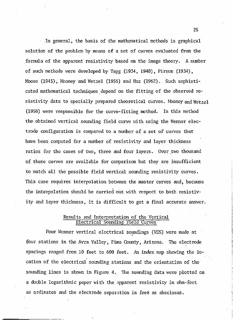
In general, the basis of the mathematical methods is graphical
solution of the problem by means of a set of curves evaluated from the
formula of the apparent resistivity based on the image theory. A number
of such methods were developed by Tagg (1934, 1940), Pirson (1934),
Moore (1945), Nboney and Wetzel (1956) and Unz (1962). Such sophisti
cated mathematical techniques depend on the fitting of the observed re
sistivity data to specially prepared theoretical curves. Nboney and Wetzel
(1956) were responsible for the curve-fitting method. In this method
the obtained vertical sounding field curve with using the Wenner elec
trode configuration is compared to a number of a set of curves that
have been confuted for a number of resistivity and layer thickness
ratios for the cases of two, three and four layers. Over two thousand
of these curves are available for comparison but they are insufficient
to match all the possible field vertical sounding resistivity curves.
This case requires interpolation between the master curves and, because
the interpolation should be carried out with respect to both resistiv
ity and layer thickness, it is difficult to get a final accurate answer.
Results and Interpretation of the Vertical Electrical Sounding Field Curves
Four Wenner vertical electrical soundings (VES) were made at
four stations in the Avra Valley, Pima County, Arizona. The electrode
spacings ranged from 10 feet to 600 feet. An index map showing the lo
cation of the electrical sounding stations and the orientation of the
sounding lines is shown in Figure 4. The sounding data were plotted on
a double logarithmic paper with the apparent resistivity in ohm-feet
as ordinates and the electrode separation in feet as abscissas.
26
[ronwood Picnic w* T. Area.i
34
7 ^
----> -r
V.-- • . • •:
Scale 1:62500 3000' 0 3000
Figure 4. Index map shelving location of the electrical verticalsounding stations and orientation of the sounding lines.

27
The significance of field sounding curves from the standpoint of
prospecting lies in the variations in the calculated apparent resistiv
ity rather than in the absolute values, and the important factor is in
the electrode separation or the depth at which a marked change occurs.
On a qualitative basis, all the sounding curves show a decrease
in the value of the apparent resistivity as the electrode spacing in
creased to about 100 feet. After the 100 feet, the apparent resistiv
ity value shows a fairly uniform increase.
The quantitative interpretation of the field VES curves was
made using albums of theoretical three-layer and four-layer master
curves (Mooney and Wetzel 1956).
The VES 1 Curve
About one mile north of Snyder Hill, at Station A, measurements
were taken to obtain the VES 1 curve (Figure 5). The electrodes were
placed on a line running approximately north-south parallel to Aldon
Road, and measurements made at an electrode interval varying from 10
feet to 450 feet. The calculated apparent resistivities of these
measurements at Stations A are shown in Table 1.
The VES 1 curve (Figure 5) was smoothed to be interpreted in
terms of horizontally stratified homogeneous media.
By using the curve-matching technique with Nfooney and Wetzel
master curves (1956), it was found that the VES 1 curve represents a
four-layer geoelectric section of the type P^:P2:p3:p4 = 1:1/3:3:1 and
= 1:3:6.

Electraratio(feet)
10204060100150200300450
TABLE 1
Calculated Apparent Resistivities at Station A
Potential Current I Apparent Self Potentialdifference, AV (Amperes) resistivity (milli-volts)
(volts) (ohm-feet)
0.859 0.20.382 0.20.331 0.40.135 0.30.103 0.40.125 0.60.117 0.650.114 0.80.0349 0.34
270 79.0240 75.0195 90.4170 100.0162 85.4196 55.2226 86.4269 38.6290 68.3
•h 400
% 200
I I I60 70 80 90 100 250 300 400 500
Electrode separation (a) in feet
Figure 5, Vertical electrical sounding curve VES 1 at Station A, N)

30
According to this interpretation, it was found that the VES 1
curve (Figure 5) indicates the presence of a thin near-surface, dry
coarse-grained alluvial layer (sand and gravel) having a resistivity
of about 255 ohm-feet and a thickness of about 28 feet. An underlying
layer having a much lower resistivity (85 ohm-feet) probably represents
clay-cemented unconsolidated alluvial layer (clayey sand). The third
layer, a more resistive layer (765 ohm-feet), occurring at a depth of
about 85 feet, probably represents water-saturated fractured bedrock
(limestone?) underlain by a layer having a resistivity of 255 ohm-feet
and it occurs at a depth of about 170 feet. This interpretation can
be summarized in a table as follows (Table 2):
TABLE 2
Interpretation of the VES 1 Curve
Layer Depth (feet) Probable Lithology Resistivity(olun-feet)
1 0- 28 Unsaturated sand and gravel
255
2 28- 85 Clayey sand 853 85-170 Fractured limestone
with water765
4 >170 Conglomerate 255
It is interesting to see how the results of the well log fit
those predicted from the geoelectrical vertical sounding survey.
About 200 feet to the west of Station A, a drilling log showed the fol
lowing at well (D-14-12) 35bdb (Table 3):

31
TABLE 3
Results of a Drilling Log at Well (D-14-12).33bdb
Depth Range (feet) Formation
0- 90 Conglomerate
90-105 Loose gravel
105-122 Conglomerate, hard, tight
122-146 ' Limestone, hard
146-152 Limestone, soft-fractured with water
152-160 Limestone, hard
160-165 Conglomerate, hard
165-175 Limestone, hard
175-210 Conglomerate, hard
210-225 Limestone, very hard
Assuming the stratigraphic sequence of the rock units at Station
A is the same as that at well (D-14-123 33bdb, then comparison between
their results indicates that the calculated depths at Station A do not
agree with the known drilling depths. The difference between the predicted
and the actual depths to the subsurface rock units may be accounted for
by the effects of small lateral inhomogeneities near the subsurface
along the line of electrodes spread, or maybe the drill had struck
a low point on an irregular rock surface.

3 2
The VES 2 Curve
The vertical sounding was made at Station B with an electrode
array oriented N50°E and the measurements run at electrode intervals
varying from 10 feet to 600 feet. The calculated apparent resistivities
of these measurements at Station B are shown in Table 4.
The VES 2 Curve (Figure 6) represents a four-layer geoelec
trical section of the type P]/P2:p3:p4 = 1'1/3:1:3 and =1:2:6.
It indicates a dry alluvial layer (sand and gravel) of 210 ohm-feet
resistivity to a depth of 45 feet, underlain by a conductive layer (70
ohm-feet) with a thickness of about 45 feet, which probably represents
clay-cemented unconsolidated alluvium. The VES 2 Curve also indicates
a third layer of resistivity 210 ohm-feet occurs at a depth of 90 feet
which probably represents water-bearing zone underlain by another layer
having a high resistivity (630 ohm-feet) occurs at a depth of about 270
feet.
The VES 3 Curve
The vertical sounding was conducted at Station C with an elec
trode array placed on a line trending east-west and the measurements
were made at electrode intervals ranging from 10 feet to 6000 feet.
The calculated apparent resistivities of this curve are shown inTable 5.
The VES 3 Curve (Figure 7) does not provide a good match to the
theoretical curves; so interpolation between curves was tried. With

TABLE 4
Calculated Apparent Resistivities at Station B
Electrode Separation, a
(feet)
Potential difference, AV
(volts)
Current(Amperes)
Apparent resistivity, (ohm-feet)
Self Potential (milli-volts)
10 1.04 0.3 218 72.720 0.364 0.2 229 108.0.40 0.226 0.3 189 90.560 0.1235 • 0.3 155 100.0100 0.066 0.3 138 92.0150 0.061 0.4 144 103.0200 0.0772 0.6 162 79.6250 0.0673 0.6 176 75.1300 0.0621 0.6 195 78.0450 0.0692 0.8 245 73.0600 0.0617 0.8 291 67.2 -
0404

1000
•8 600
2 200
a iso
400 500 600250 30025 30 60 70 80 90 100Electrode separation fa) in feet
Figure 6. Vertical electrical sounding curve VES 2 at Station B.

aratio(feet)
10204060100150
'200300450600
TABLE 5
Calculated Apparent Resistivities at Station C
Potential Current Apparent Self Potentialdifference, AV (Amperes) resistivity, (milli-volts)
(volts). (ohm-feet)
2.04 0.4 321 61.40.641 0.3 269 13.30.252 0.3 211 98.40.211 0.4 199 112.00.1635 0.4 257 114.00.128 0.4 302 85.00.108 0.4 339 76.70.0832 0.4 392 69.00.0541 0.4 383 48.70.0417 0.4 393 33.1
04Cn

Apparent resistivity (p ) in ohm-feet
I I >SO 60 70 80 90 100 250 300 500 600
Electrode separation (a) in feet
Figure 7. Vertical electrical sounding curve VES 3 at Station C.

37
such interpolation it was found that the VES 3 curve represents a four-
layer geoelectrical section of the type pi;P2:p3:p4 = 1:1/3:3:1 and
between 1:2:6 and 1:3:6.
According to this, the VES 3 curve was interpreted as follows:
TABLE 6
Interpretation of the VES 3 Curve
Layer Depth (feet) Probable Lithology Resistivity(ohm-feet)
1 0- 23 Dry sand and gravel 305
2 23- 56 Clay-cemented material 102
3 56-135 Fractured limestone with water
915
4 >135 Conglomerate ? 305
The VES 4 Curve
The vertical sounding was made at Station D with an electrode
array oriented N60°E and measurements were done at electrode intervals
varying from 10 feet to 600 feet.
The calculated apparent resistivities of the measurements at
Station D are shown in Table 7.
It was found that the VES 4 curve (Figure 8) may represent
either a four-layer geoelectric section of the type =
1:1/3:1:10 and :D2" = 1:3:6 or a three-layer section of the type
P1 P2 P3 — and = 1:4.

TABLE 7
Calculated Apparent Resistivities at Station D
Electrode Separation, a
(feet)
Potential difference, AV
(volts)
Current(Amperes)
Apparent resistivity,pa
(ohm-feet)
10 1.051 0.2 33015 0.665 0.2 31420 0.469 0.2 29525 0.493 0.28 27630 0.281 0.2 26540 0.1922 0.2 24250 0.1368 0,2 21560 0.106 0.2 200100 0.0542 0,2 170ISO 0.0404 0.2 190200 0,0373 0.2 234300 0.0374 0.22 321400 0.0355 0.22 406500 0.0523 0.34 483600 0.0371 0.24
00
Apparent resistivity (p ) in ohm-feet
I I l50 60 .70 80 90 100 200 250 300 400 500 600Electrode separation (a) in feet
Figure 8. Vertical electrical sounding curve VES 4 at Station D.
8

40
Hie first interpretation of the VES 4 curve with relative to the
four-layer case, is as follows:
TABLE 8
First Interpretation of the VES 4 Curve
Layer Depth (feet) Probable Lithology Resistivity(ohm-feet)
1 0- 36 Dry sand and gravel 300
2 36-108 Clay-cemented material 100
3 108-215 Water-bearing layer 300
4 >215 Bedrock (limestone ?) 3000
The second interpretation, with relative to the three-layer case,
is as follows:
TABLE 9
Second Interpretation of the VES 4 Curve
Layer Depth (feet) Probable Lithology Resistivity(ohm-feet)
1 0- 35 Dry sand and gravel 305
2 35-140 Clay-cemented material 102
3 >140 Bedrock (limestone ?) 3050

CHAPTER 4
HORIZONTAL PROFILING.
Introduction
The objective of the present section is to summarize the theoreti
cal treatment used in solving the detection of the structural disconti
nuity problem and to show how the theoretical results can be used to
interpret field data obtained with Wenner electrode configuration.
One of the problems in interpreting field resistivity data is to
recognize what approximations can be made in order to fit the theoreti
cal profiles satisfactory to the field curves. Computations of the
theoretical resistivity anomalies ever different types of structural
discontinuities are so difficult that reasonable approximations in the/
interpretation are highly desirable:
When an electric current passing from a formation characterized
by a certain conductivity into another one whose conductivity is dif
ferent, a distortion will appear in the form of the equipotential lines.
The result is similar to what occurs when a ray of light passes from one
medium into another of different index of refraction. This phenomenon is
well shown on the horizontal profiles of resistivity. In such electrical
horizontal resistivity profiling survey changes in structure and lithol
ogy (e.g., faults, dikes, veins and other similar structural discon
tinuities) are usually detected using a constant spacing system. This
was done by keeping the distance between the electrodes constant and41
42
moving all the electrodes along a certain line of traverse. Such type of
survey is called longitudinal traverse survey.
Actually, the apparent resistivity, as measured by the Wenner
longitudinal traverse profiling method, is quite irregular in its relation
to the structural discontinuities. No definite relation exists that can
be applied for finding their positions on the electrical resistivity
profiles. Generally, a very abrupt change of resistivity may indicate
a geologic structure, or it may not, since some irregularities are not
associated with structural discontinuities. Faults could be discovered
especially if the rock units on the opposite sides are different, or if
there is a considerable shear zone associated with the fault plane.
At any point, relative to the structural discontinuity, the
value of the apparent resistivity pa is a function of the resistivities
of the two media, of the electrode separation (a), of the distance of
the configuration*s center from the discontinuity and of the angle at
which the electrodes are aligned with respect to the discontinuity. The
actual detectability of a buried structural discontinuity depends not
only upon the thickness of the overburden, but also upon the resistivity
of the overburden in relation to the resistivity contrast of the materials
on either side of the discontinuity.
Tagg (1930) computed theoretical horizontal resistivity profiles
across a vertical fault with the Wenner electrode configuration along
a traverse perpendicular to the fault plane. He found that for all
resistivity contrasts, the principal peak lies a distance of j from
the fault, and its apparent resistivity is always less than the true

43
resistivity of the more resistive medium. The fault lies this distance
in a down-resistivity direction from the peak.
Hubbert (1934) carried out some measurements on an experimental
traverse profile across a piece of sheet metal immersed in water instead
of the ground. Stations were taken din apart with an electrode separa
tion "aM equal to din. He found that when the metal sheet was placed
midway between the potential electrodes at right angles to the line of
the electrodes the apparent resistivity p& was greater than the normal
resistivity. When the electrodes were moved so that the sheet was be
tween a potential electrode and a current electrode the apparent resis
tivity pa was less than the normal resistivity; and finally, as the
electrodes were moved away from the sheet the apparent resistivity
Pa approached the normal value.
Theoretical horizontal resistivity profiles with the Wenner
electrode configuration across vertical perfectly conducting and in
sulating planes studied by Howell (1934) are shown in Figure 9. For
the perfectly insulating plane, a minimum in the central region of
the anomaly, with an apparent resistivity value equal to three times
that of the surrounding country rock, is obtained as the center of
the Wenner configuration lies vertically over the plane. For the
vertical perfectly conducting plane, a typical W-shaped curve is ob
tained, and an apparent resistivity value equal to that of the sur
rounding rock is observed as the center of the Wenner configuration
lies vertically over the plane.

44“ A "
: 1i
Perfectly in-'•sulstting-6 -5-4-3-2-1 x 1 2 345-6
Perfectly. . . I conducting . . |
Figure 9. Theoretical horizontal resistivity profiles across vertical perfectly insulating and conducting planes with the Wenner configuration. --(After Howell 1934.)

45
Heiland (1934) made brief model studies to test the validity
of the theoretical horizontal resistivity curves using the Wenner elec
trode configuration over a perfectly conducting and insulating sheet
planes dipping at angles of 0°, 30°, 60°, and 90°. He found for a
vertical perfectly conducting plane, the apparent resistivity curve is
symmetrically W-shaped similar to the theoretical apparent resis
tivity curve in Figure 9B; and the value of the apparent resistivity
at the top of the central peak is approximately equal to the true
resistivity of the tank fluid. For a perfectly conducting plane with
a 60° dip, the "W" is somewhat symmetrical, and the apparent resistiv
ity value of the lower right part of the "W" is lower than that of the
corresponding part of the curve for a vertical plane. For a dip of
30°, the assymmetry of the curve is more pronounced, and the "W" leans
to the right.
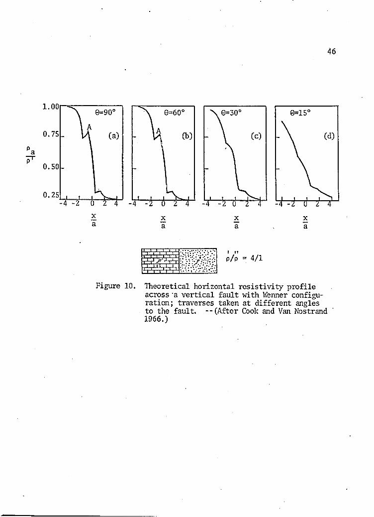
Figure 10 shows theoretical horizontal resistivity profiles
across a vertical fault with the Wenner electrode configuration along
traverses taken at different angles to the fault. The assumed resis-I It
tivity contrast is p/p = 4:1.
Figure 11 shows a theoretical horizontal resistivity profile
with the Wenner electrode configuration along a traverse perpendicular
to the strike of a fault dipping 45°. The general shape of the curve
is similar to that for a vertical fault (Figure 10). For example, peak
A lies a distance of from the outcrop of the trace of the inclined
fault, as in the case of the vertical fault. For the vertical fault
(Figure 10 ), peak A theoretically has a value equal to that of the
46
i ii ii-4-0 > J-rV m ! ft
p/p 4/1
Figure 10. Theoretical horizontal resistivity profile across a vertical fault with Wermer configuration ; traverses taken at different angles to the fault. -- (After Cook and Van Nostrand 1966.)

47
-4 -3 -2xa
ftuif-H - i 1 ; <
Figure 11. Theoretical horizontal resistivity profile with Wermer configuration along traverse perpendicular to strike of fault dipping 45°, --(After Cook and van Nostrand 1966.)

48country rock while in the present dipping-fault model, peak A is of
much higher value than for the vertical fault of the same resistivity
contrast.
Analysis of the Profiling Data
The purpose of the horizontal resistivity profiling survey,
conducted in Avra Valley, Pima County, Arizona, was to locate the posi
tion of a subsurface scarp that separates a pediment surface obscured
by shallow alluvial cover from the area where the thickness of alluvium
is much greater.
The discussion of the horizontal resistivity profiles which
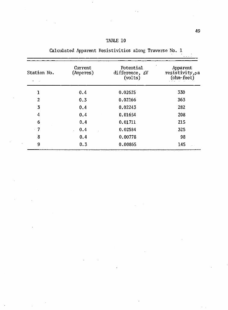
constitute the second main part of this paper is based entirely upon
the results of the calculated apparent resistivities shown in Tables
10 to 12. The Wenner electrode configuration was used in the horizon
tal profiling survey. All of the traverses were made with a constant
electrode spacing of "a" equal to 800 feet and the successive stations
were spaced at intervals of 800 feet. An index map showing the loca
tion of the horizontal resistivity lines is shown in Figure 12.
The graphs of the horizontal resistivity profiles shown in
Figures 13 to 15 are plotted with apparent resistivities in ohm-feet
as ordinates and with distances divided into stations at 800-feet
intervals as abscissas. The apparent resistivity was plotted at the
midpoint between the potential electrodes p^ and p^.
49
TABLE 10
Calculated Apparent Resistivities along Traverse No. 1
Current Potential ApparentStation No. (Amperes) difference, AV resistivity,pa
(volts) (ohm-feet)
1 0.4 0.02625 3302 0.3 0.02166 3633 0.4 0.02243 2824 0.4 0.01654 2086 0.4 0.01711 2157 . 0.4 0.02584 3258 0.4 0.00778 989 0.3 0.00865 145

50
TABLE 11
Calculated Apparent Resistivities along Traverse No. 2
Station No.Current(Amperes)
Potential difference, AV
(volts)
Apparent resistivity,
(ohm-feet)
1 0.4 0.02162 2722 0.4 0.02280 2873 0.4 0.02105 2654 0.5 0.02210 2225 0.26 0.00973 1886 0.4 0.01485 1877 0.5 0.03440 3468 0.4 0.00789 999 0.4 0.01153 14510 0.4 0.01893 238

51TABLE 12
Calculated Apparent Resistivities along Traverse No. 3
Station No.
Current(Amperes)
Potential difference, AV
(volts)
Apparent resistivity,
(ohm-feet)
1 0.3 0.01759 2952 0.2 0.01280 3223 0.2 0.00664 1674 0.2 0.00495 1245 0.4 0.00931 1176 0.4 0.00757 957 0.2 0.00415 104
r

52
34
L X
•A S.,8
v- -
Scale 1:62500 3000' 0
Figure 12. Index map sliowing location of the electrical horizontal profiling stations and orientation of theprofiling lines.

Elevation
(feet)
Apparent resistivity (p ) in ohm- f
eet
800 1600 2400 3200 4000 4800 5600 6400 7200 8000Distance in feet
Alluvium
Figure 13. Horizontal resistivity profile No. 1 with twodimensional model used for interpretation.--Electrode separation a = 800 feet; stationinterval = 800 feet.

54
•H 300
.3 200
9 * 100
1600 2400 3200 4000 4800 5600 6400 7200 8000Distance in feet
Alluviumti 200
5 1500
Figure 14. Horizontal resistivity profile No. 2 with twodimensional model used for interpretation.--Electrode separation a = 800 feet; stationinterval = 800 feet.

Elevation
(feet)
Apparent resistivity (pa) in ohm-feet
1600 2400 3200 4000 4800 5600 6400 7200 8000Distance in feet
2000 7Alluvium
1500.
1000.
Figure 15. Horizontal resistivity profile No. 3 with twodimensional model used for interpretation. --Electrode separation a=800 feet; station interval = 800 feet.
56
The horizontal resistivity profiling survey was taken in dry
weather over a sun-baked ground; consequently, a number of the ground
contacts were very poor. No correction for this was applied in the
computations, so that the minor variations in the curves may be due
to this cause.
Interpretation of the field horizontal profiles was based on
a careful correlation with some of the theoretical horizontal resis
tivity profiles computed from mathematical apparent resistivity formu
las derived through the applications of theory of image. The field
profiles were also compared with other field horizontal resistivity
curves done by some workers over well known faults in certain areas.
The first thought may lead one to believe that detection of
structural discontinuities, such as a fault, would be geophysically
simple, since the fault represents a stratigraphic displacement, so
that the material on opposite sides of the fault would be different
and the apparent resistivity on one side is different from the ap
parent resistivity on the other side. This concept was used by
Hubbert (1934). Actually, the problem is much more difficult, be
cause there are many changes of resistivity so that it becomes a prob
lem of discovering these particular changes, which are special signals
to the geologic structures under examination. Another special diffi
culty lies in the fact that the surface of the ground in the investi
gated area is covered with alluvium, so not much detailed information
could be recognized as an indication for anticipating faults.

Figures 13, 14 and 15 show the field horizontal resistivity
curves with the Wenner electrode configuration. In all cases, the
electrode separation is 800 feet, and the station interval is 800 feet.
The lengths of these longitudinal horizontal profiles are 6400, 6400,
and 4400 feet. The apparent resistivity on the three horizontal pro
files is about 250 to 350 ohm-feet over the bedrock and about 100 ohm-
feet or less over the contact area.
The peak at A and the trough at B on the horizontal resistiv
ity curves are the most spectacular anomalies obtained in the investi
gated area. The essential characteristics of the anomaly are: 1) when
the bedrock-alluvium contact (it is suggested by the author to call
this contact a bedrock shelf, which may represent just a face of struc
tural discontinuity) was located between the current electrode and
the potential electrode p^ the apparent resistivity p& is relatively
higher than the surrounding normal values, and 2) when the bedrock
shelf was located between the two potential electrodes p^ and P2» the apparent resistivity p& is very low. This produced in the field hori
zontal resistivity curves a sort of asymmetrical W shape. The lack
of symmetry may be due to the lack of uniformity in the degree of
packing of the subsurface earth materials or to inhomogeneity effects.
The abrupt change in slope of the three curves occurs as the po
tential electrodes p^ and p^ cross the bedrock-alluvium contact. The
total change from the peak at A to the minimum at B occurs over a horizontal distance equal to the electrode separation, i.e., equal to
57
800 feet.

58
The secondary peaks and lows on the field horizontal profiling
curves are probably caused by some other lateral changes in the sub
surface earth materials.
Interpretation of the field data was based on a comparison of
the field curves with theoretical horizontal resistivity profiles, as
well as with other field horizontal resistivity curves conducted by
other workers.
The general features of the peaks and troughs in the field
curves are similar to those in the theoretical horizontal resistivity
profiles (Figures 10 and 11).
The theoretical curves are continuous smooth curves. But in
the field work, the curves need not be smooth. If the points were
connected by the most reasonable continuous curve, we would find that
even in the ideal case the characteristic points on the field curve
would not match the corresponding points on the theoretical curve.
Therefore, to get a good match between the field curves and the
theoretical horizontal resistivity profiles, it was found convenient
to plot the theoretical curves again rather than smoothing the field
curves. Plotting the theoretical curves again was done by taking dis
crete points from the theoretical horizontal resistivity profiles and
connecting them with straight lines. The spacing of the discrete points
was made equal to the station interval along the horizontal resistivity
traverse in the field. The curves obtained by this procedure are called
theoretical field curves (i.e., field plot of the theoretical data).

59
The theoretical field horizontal resistivity curves are helpful in
exhibiting the sharp peaks and troughs that make the comparison easier.
In Figures 16 and 17 the field horizontal curves were compared
with the theoretical field curves of a vertical and dipping faults.
The theoretical field curves were plotted in the usual manner at the
station which occupies the midpoint between the potential electrodes
p^ and P2, with the spacing between successive stations being equal to the whole electrode separation "a." Good resemblance was obtained
from such conparison.
In the transition area to the right of peak A on the field
curves, the steep slope is somewhat similar to the theoretical field
profiles. Therefore, the bedrock-alluvium contact theoretically lies
as much as or 400 feet to the east of peak A on the field curves.
It was also considered that the pronounced apparent resistivity low
at B-might be caused by saturated fault gouge material accumulated
along the bedrock shelf.
This estimate of the location of the alluvium-bedrock contact
is an approximate one, since the structural discontinuity along the con
tact does not extend to infinite depth, as assumed in the theoretical
horizontal resistivity profiles, and the resistivity contrast may not be
exactly 1 to 4. However, more precise determination of the location of
the alluvium-bedrock contact can be obtained by taking smaller spacing
of the stations which may be worth the extra time and trouble during
the field work.

Apparent resistivity in ohm-feet
60
Station
iy 1:1: m mFigure 16. Comparison of theoretical field and observed
field horizontal resistivity profiles; (a)observed field curve No. 1. (b) observed field curve No. 2 (c) theoretical field plotover a fault.

Apparent resistivity in ohm-feet
61
1 2 3 4 5 6 7 8 9 10 Station
1 2 3 4 .5 6 7 8 9 10Station
Figure 17. Comparison of theoretical field andobserved field horizontal resistivity profiles; (a) observed field curveNo. 3 (b) theoretical field plot over a fault dipping 45°.

62
Based upon the comparison of the field curves with the theoreti
cal resistivity profiles, the line that connects the points a, b,
and c along the three resistivity profiling lines in Figure 12 marks
the probable position of a subsurface structural discontinuity (pro
bably subsurface fault scarp, which produced the pronounced low apparent
resistivity value on the field curves. The strike of this scarp is
about N30°W.
This inferred subsurface fault may be one of the marginal
north-northwest basin-range faults which are responsible for the present
mountain-valley pattern. Such marginal faults, which covered by alluvi
um, must be present to form a resultant series of downthrown blocks
progressing in the western direction from the Tucson Mountains.
From the point of view of depth to bedrock, the sharp decrease
in the apparent resistivity value on the horizontal field profiling
curves indicates that the depth to the bedrock increases rapidly west
of the subsurface fault scarp. East of this scarp alluvial deposits
are approximately 100 to 300 feet thick, and west of it the alluvium
shows a rapid increase in thickness which may reach 5,000 feet in the
central part of the valley, as in the Ryan Field area. . Data from
wells (White et al. 1966) substantiate this interpretation in several
locations.
According to this interpretation, it is suggested that the
nortli-northwest trending electrical resistivity anomaly southwest of
the Tucson Mountains is probably caused by a subsurface scarp, striking
N30°W, that may be the result of a steeply dipping normal fault.

63Previous geophysical and geological work conducted in the
Avra Valley support the discussion given above. Heindl (1959) inter
preted the rapid changes in the water-level altitudes northwest of
the Del Bac Hills as large north-northwest trending faults which
separate the basin and range blocks. Plouff (1961) noted a linear
gradient in the Bouguer anomaly west of the Tucson Mountains, and suggested that this probably indicates the presence of subsurface base
ment scarps that may be the result of faulting. A gravity survey con
ducted by West (1970) in the Avra Valley shows pronounced gravity highs
over the west part of the Sierrita and Tucson Mountains. A northeast
trending line of gravity lows extends to the northwest of the Sierrita
Mountains and then turns to the northwest near the Ryan Field. These
gravity lows follow the trends of Altar and Avra valleys. He found
that the gravity anomaly southwest of the Tucson Mountains trends north-
northwest. A similar trend occurs on the west side of Avra Valley,
but its magnitude and gradient are much smaller than those on the east
side of the valley. West (1970) found that the largest gradient occurs
2.5 miles northwest of the Ryan Field on State Highway 86 where a
12 mgal change occurs in the residual gravity anomaly in a distance
of one mile. He suggested that the north-northwest trending gravity
anomaly southwest of the Tucson Mountains is probably cuased by a sub
surface fault scarp.

CHAPTER 5
CONCLUSIONS
The success of the field work in geoelectrical resistivity
survey depends on how well we may be able to understand the language
in which the rocks speak to us through this method.
Four layers with contrasting electrical resistivities and
thicknesses were recognized in the vertical sounding survey. The upper
most layer correlated with unsaturated alluvium, underlain by a layer
with a lower resistivity, which probably represents clay-cemented un
consolidated alluvium. The third and fourth layers were considered to
be indicative of saturated material to probably basement rocks.
Based on the interpretation of the horizontal field profiling
curves, it was suggested that the north-northwest trending electrical
resistivity anomaly southwest of the Tucson Mountains is probably caused
by a subsurface scarp that may be the result of a steeply dipping normal
fault. . The strike of this scarp is about N30°IV.
It should be emphasized that a thorough study of the subsurface
stratigraphic sequence of the rock units and their structural relations
is essential for a satisfactory interpretation of the horizontal re
sistivity profiling anomaly, to be sure that such fluctuations in the
horizontal resistivity profiles are not produced by other geological
factors.
64
I
65
The obtained results of this geoelectrical survey may give
useful service to irrigation and civil engineering projects; since
these engineering fields always require information on depth to bed
rock, to gravel, or clay layers.
From the point of view of depth to bedrock, shallow buried
bedrock occurs to the east of the subsurface fault scarp, and west of
it the bedrock surface is very deep. East of the scarp alluvial deposits
are about 100 to 300 feet thick, and west of it the alluvium shows a
rapid increase in thickness which may reach 5000 feet in the central
part of the valley, as in the Ryan Field area.
This inferred fault scarp may put some limitations upon the
selection of an area for mineral exploration since the depth to bed
rock beyond this scarp is very large. Most mineral exploration in the
Avra Valley area has been carried out on portions of the shallow buried
bedrock surface (i.e., pediment surface). On the other hand, the pedi
ment area cannot provide large supplies of ground water because of the
limited thickness of the alluvial deposits.
Withdrawal of ground water from the Avra Valley increases the
possibility of general basin subsidence which may result in structural
failures of roads and foundations. Areas close to subsurface fault
scarp are particularly susceptible to this type of damage because of
differential subsidence. On this basis, the probability that damage of
tliis sort will be great for structures which are going to be built
near this inferred subsurface fault scarp area.

LIST OF REFERENCES
Bennett, P. J., 1957, The geology and mineralization of the Sedimentary Hills area, Pima County, Arizona: Unpubl. M.S. Thesis, Univ.of Arizona, 45 p.
Bikerman, M., 1962, A geologic-geochemical study of the Cat Mountain Rhyolite: Unpubl. M.S. Thesis, Univ. of Arizona, 43 p.
Bikerman, M., 1963, Origin of the Cat Mountain Rhyolite: ArizonaGeological Society Digest, V. 6, p. 83-89.
Bikeiman, M. and Damon, P., 1966, K-Ar chronology of the TucsonMountains, Pima County, Arizona: Geol. Soc. Am. Bull., V. 77,p. 1225-1234.
Britt, T. L., 1955, The geology of the Twin Peaks area, Pima County, Arizona: Unpubl. M.S. Thesis, Univ. of Arizona, 58 p.
Brown, W. H., 1939, Tucson Mountains, an Arizona Basin Range type:Geol. Soc. Am. Bull., V. 50, p. 697-760.
Bryan, K., 1925, The Papago County, Arizona: U.S. Geol. Survey, WaterSupply Paper 499, p. 93.
Bryant, D. L., 1955, Stratigraphy of the Permian system in southernArizona: Unpubl. Ph.D. Dissertation, Univ. of Arizona, 209 p.
Colby, R. E., 1958, The stratigraphy and structure of the RecreationRed Beds, Tucson Mountains Park, Arizona: Unpubl. M.S. Thesis,Univ. of Arizona, 64 p.
Cook, K. L. and Van Nostrand, R. G., 1966, Interpretation of resistivity data: Geol. Survey Prof. Paper 499, U.S. Govt. PrintingOffice, 310 p.
Damon, P. E., 1967, Correlation and chronology of ore deposits: U.S.Atomic Energy Commission Progress Report (COO-689-76).
Davenport, R. E., 1963, Geophysical investigation of the Sedimentary Hills area, Pima County, Arizona: Unpubl. M.S. Thesis, Univ.of Arizona, 51 p.
Flathe, H., 1955, Possibilities and limitations in applying geoelectrical methods to hydrological problems in the Coastal Areas of North West Germany: Geophysical Prospecting, 3, p. 95-110.
66

67
Gish, 0. H. and Rooney, W. J., 1925, Measurement of resistivity of large masses of undisturbed earth: Terr. Mag. Atom. Elec.,V. 30, p. 161-188.
Holland, C. A., 1934, Geophysics in the nonmetallic field: Trans.Amor. Inst. Mining Met. Engrs., V. 110, p. 546-577.
Heindl, L. A., 1959, Geology of the San Xavier Indian Reservation, Arizona: Arizona Geol. Soc., Guidebook II, p. 152-159.
Howell, L. G., 1934, Discussion to paper by M. K. Hubbert: Trans.Amer. Inst. Mining Met. Engrs., V. 110, p. 34-37.
Hubbert, M. K., 1934, Results of earth-resistivity survey on various geologic structures in Illinois: Trans. Amer. Inst. MiningMet. Engrs., V. 110, p. 9-39.
Kinnison, J. E., 1958, Geology and ore deposits of the southern section of the Amole Mining District, Tucson Mountains, Pima County, Arizona: Unpub 1. M.S. Thesis, Univ. of Arizona, 123 p.
Lancaster-Jones, E., 1930, the earth-resistivity method of electrical prospecting: Mining Mag., V. 42, p. 352-355.
Mayo, E. B., 1963, Volcanic orogens of the Tucson Mountains: ArizonaGeol. Soc. Digest, V. 6, p. 61-82.
Mayo, E. B., 1968, A history of geologic investigation in the TucsonMountains, Pima County,-Arizona: Arizona Geol. Soc. GuidebookIII, p. 155-170.
Mooney, H. M. and Wetzel, W. W., 1956, The potentials about a point electrode and apparent resistivity curves for a two-, three- and four layer earth: Univ. of Minnesota Press, Minneapolis,146 p., plus reference curves.
Moore, R. W., 1945, An empirical method of interpretation of earth resistivity measurements: Trans. Amer. Inst. Mining Met.Engrs., V. 164, p. 197-223.
Pirson, S. J., 1934, Interpretation of three-layer resistivity curves: Trans. Amer. Inst. Mining Met. Engrs., V. 110, p. 148-158.
Plouff, D., 1961, Gravity survey near Tucson, Arizona: U.S. Geol.Survey Prof. Paper 424-D, p. D258-259.

68
Tagg, G. F., 1930, The earth resistivity method of geophysical prospecting: Mining Mag., V. 43, p. 150-158.
Tagg, G. F., 1934, Interpretation of resistivity measurements: Trans.Amer. Inst. Mining Met. Engrs., V. 110, pi 135-147.
Tagg, G. F., 1940, Interpretation of earth-resistivity curves: Trans.Amer. Inst. Mining Met. Engrs., V. 138, p. 399-407.
Unz, M., 1962, Linear approximation of apparent resistivity functions: Geophysics, V. 27, p. 100-108.
West, R. E., 1970, Analysis of gravity data from the Avra Valley area, Pima County, Arizona: Unpiibl. M.S. Thesis, Univ. of Arizona,73 p.
White, N. D., Matlock, W. G. and Schwalen, H. C., 1966, An appraisal of the ground-water resources of Avra and Altar Valleys, Pima County, Arizona: Arizona State Land Dept. Water ResourcesReport No. 25, 66 p.
Whitney, R. L., 1957, Stratigraphy and structure of the northeastern part of the Tucson Mountains: Unpubl. M.S. Thesis, Uhiv. ofArizona, 61 p.

4 65 19