APPLIED GEOPHYSICS

Abdullah M. Al-Amri

Dept. of Geology & Geophysics

King Saud University, Riyadh

alamri.geo@gmail.com

www.a-alamri.com

2018

ELECTRICAL RESISTIVITY TECHNIQUES

Geophysical resistivity techniques are based on the response of the earth to

the flow of electrical current. In these methods, an electrical current is passed

through the ground and two potential electrodes allow us to record the resultant

potential difference between them, giving us a way to measure the electrical

impedance of the subsurface material. The apparent resistivity is then a function of

the measured impedance (ratio of potential to current) and the geometry of the

electrode array. Depending upon the survey geometry, the apparent resistivity data

are plotted as 1-D soundings, 1-D profiles, or in 2-D cross-sections in order to look

for anomalous regions.

In the shallow subsurface, the presence of water controls much of the

conductivity variation. Measurement of resistivity (inverse of conductivity) is, in

general, a measure of water saturation and connectivity of pore space. This is

because water has a low resistivity and electric current will follow the path of least

resistance. Increasing saturation, increasing salinity of the underground water,

increasing porosity of rock (water-filled voids) and increasing number of

fractures (water-filled) all tend to decrease measured resistivity. Increasing

compaction of soils or rock units will expel water and effectively increase

resistivity. Air, with naturally high resistivity, results in the opposite response

compared to water when filling voids. Whereas the presence of water will reduce

resistivity, the presence of air in voids should increase subsurface resistivity.

Resistivity measurements are associated with varying depths depending on

the separation of the current and potential electrodes in the survey, and can be

interpreted in terms of a lithologic and/or geohydrologic model of the subsurface.

Data are termed apparent resistivity because the resistivity values measured are

actually averages over the total current path length but are plotted at one depth

point for each potential electrode pair. Two dimensional images of the subsurface

apparent resistivity variation are called pseudosections. Data plotted in cross-

section is a simplistic representation of actual, complex current flow paths.

Computer modeling can help interpret geoelectric data in terms of more accurate

earth models.

Geophysical methods are divided into two types : Active and Passive

Passive methods (Natural Sources): Incorporate measurements of natural

occurring fields or properties of the earth. Ex. SP, Magnetotelluric (MT), Telluric,

Gravity, Magnetic.

Active Methods (Induced Sources) : A signal is injected into the earth and then

measure how the earth respond to the signal. Ex. DC. Resistivity, Seismic

Refraction, IP, EM, Mise-A-LA-Masse, GPR.

DC Resistivity - This is an active method that employs measurements of

electrical potential associated with subsurface electrical current flow

generated by a DC, or slowly varying AC, source. Factors that affect the

measured potential, and thus can be mapped using this method include the

presence and quality of pore fluids and clays. Our discussions will focus

solely on this method.

Induced Polarization (IP) - This is an active method that is commonly

done in conjunction with DC Resistivity. It employs measurements of the

transient (short-term) variations in potential as the current is initially

applied or removed from the ground. It has been observed that when a

current is applied to the ground, the ground behaves much like a capicitor,

storing some of the applied current as a charge that is dissipated upon

removal of the current. In this process, both capacity and electrochemical

effects are responsible. IP is commonly used to detect concentrations of

clay and electrically conductive metallic mineral grains.

Self Potential (SP) - This is a passive method that employs measurements

of naturally occurring electrical potentials commonly associated with the

weathering of sulfide ore bodies. Measurable electrical potentials have

also been observed in association with ground-water flow and certain

biologic processes. The only equipment needed for conducting an SP

survey is a high-impedance voltmeter and some means of making good

electrical contact to the ground.

Electromagnetic (EM) - This is an active method that employs

measurements of a time-varying magnetic field generated by induction

through current flow within the earth. In this technique, a time-varying

magnetic field is generated at the surface of the earth that produces a

time-varying electrical current in the earth through induction. A receiver

is deployed that compares the magnetic field produced by the current-

flow in the earth to that generated at the source. EM is used for locating

conductive base-metal deposits, for locating buried pipes and cables, for

the detection of unexploded ordinance, and for near-surface geophysical

mapping.

Magnetotelluric (MT) - This is a passive method that employs

measurements of naturally occurring electrical currents, telluric currents,

generated by magnetic induction of electrical currents in the ionosphere.

This method can be used to determine electrical properties of materials at

relatively great depths (down to and including the mantle) inside the

Earth. In this technique, a time variation in electrical potential is

measured at a base station and at survey stations. Differences in the

recorded signal are used to estimate subsurface distribution of electrical

resistivity.

Position of Electrical Methods in:

(1) Petroleum Exploration.

The most prominent applications of electrical techniques in petroleum expl.

Are in well logging. Resistivity and SP are standard Logging techniques.

The magnetotelluric method has found important application for pet.

Exploration. In structurally complex region (EX. Rocky Mountains).

(2) Engineering & Groundwater.

D C. Resistivity and EM have found broad use in civil Engineering and

groundwater studies. Saturated / Unsaturated, Saltwater / freshwater

(3) Mineral Exploration.

Electrical methods interpretation difficult below 1000 to 1500 ft. Electrical

exploration methods are the dominant geophysical tools in Mineral Expl.

Ohm’s Law

Ohm’s Law describes the electrical properties of any medium. Ohm’s Law,

V = I R, relates the voltage of a circuit to the product of the current and the

resistance. This relationship holds for earth materials as well as simple circuits.

Resistance( R), however, is not a material constant. Instead, resistivity is an

intrinsic property of the medium describing the resistance of the medium to the

flow of electric current.

Resistivity ρ is defined as a unit change in resistance scaled by the ratio of a

unit cross-sectional area and a unit length of the material through which the current

is passing (Figure 1). Resistivity is measured in ohm-m or ohm-ft, and is the

reciprocal of the conductivity of the material. Table 1 displays some typical

resistivities.

Note that, in Table 1, the resistivity ranges of different earth materials

overlap. Thus, resistivity measurements cannot be directly related to the type of soil

or rock in the subsurface without direct sampling or some other geophysical or

geotechnical information. Porosity is the major controlling factor for changing

resistivity because electricity flows in the near surface by the passage of ions

through pore space in the subsurface materials. The porosity (amount of pore

space), the permeability (connectivity of pores), the water (or other fluid) content

of the pores, and the presence of salts all become contributing factors to changing

resistivity. Because most minerals are insulators and rock composition tends to

increase resistivity, it is easier to measure conductive anomalies than resistive ones

in the subsurface. However, air, with a theoretical infinite resistivity, will produce

large resistive anomalies when filling subsurface voids.

Electric circuit has three main properties:

o Resistance (R): resistance to movement of charge

o Capacitance (C): ability to store charge

o Inductance (L): ability to generate current from changing magnetic

field arising from moving charges in circuit

Resistance is NOT a fundamental characteristic of the metal in the wire.

MECHANISM OF ELECTRICAL CONDUCTION

Mechanism of electrical conduction in Materials the conduction of

electricity through materials can be accomplished by three means :

a) The flow of electrons Ex. In Metal

b) The flow of ions Ex. Salt water .

c) Polarization in which ions or electrons move only a short distance under

the influence of an electric field and then stop.

1 Metals :

Conduction by the flow of electrons depends upon the availability of free

electrons. If there is a large number of free electrons available, then the

material is called a metal, the number of free electrons in a metal is roughly

equal to the number of atoms.

The number of conduction electrons is proportional to a factor

n ≈ ε E/KT E ∞ 1/n T ∞ n

ε : Dielectric constant

K: Boltzman’s constant

T: Absolute Temperature.

E Activation Energy.

Metals may be considered a special class of electron semi conductor for

which E approaches zero.

Among earth materials native gold and copper are true metals. Most sulfide

ore minerals are electron semi conductors with such a low activation energy.

b) The flow of ions, is best exemplified by conduction through water,

especially water with appreciable salinity. So that there is an abundance of

free ions.

Most earth materials conduct electricity by the motion of ions contained in

the water within the pore spaces .

There are three exceptions :

1) The sulfide ores which are electron semi conductors.

2) Completely frozen rock or completely dry rock.

3) Rock with negligible pore spaces ( Massive lgneous rooks like gabbro . It

also include all rocks at depths greater than a few kilometers, where pore

spaces have been closed by high pressure, thus studies involving

conductivity of the deep crust and mantle require other mechanisms than

ion flow through connate water.

c) Polarization of ions or sometimes electrons under the influence of an

electrical field, they move a short distance then stop. Ex. Polarization of the

dielectric in a condenser polarization ( electrical moment / unit volume)

Conductivity mechanism in non-water-bearing rocks

1) Extrinsic conductivity for low temperatures below 600-750o k.

2) Intrinsic conductivity for high temperatures.

Most electrical exploration will be concerned only with temperatures well below

600-750o . The extrinsic is due to weakly bonded impurities or defects in the

crystal . This is therefore sensitive to the structure of the sample and to its

thermal history .

Both of these types of conductivity present the same functional form, hence

conductivity vs. temperature for semi conductors can be written :

σ = Ai ε – Ei/RT + Ae ε – Ee/RT

Ai and Ae : Numbers of ions available . Ai is 105 times Ae

Ei and Ee are the activation energies . Ei is 2 times as large as Ee .

R: Boltzman’s constant

ELECTRICAL PROPERTIES OF ROCKS :

Resistivity (or conductivity), which governs the amount of current that passes

when a potential difference is created.

Electrochemical activity or polarizability, the response of certain minerals to

electrolytes in the ground, the bases for SP and IP.

Dielectric constant or permittivity. A measure of the capacity of a material to

store charge when an electric field is applied . It measure the polarizability of a

material in an electric field = 1 + 4 π X

X : electrical susceptibility .

Electrical methods utilize direct current or Low frequency alternating current to

investigate electrical properties of the subsurface.

Electromagnetic methods use alternating electromagnetic field of high frequencies.

Two properties are of primary concern in the Application of electrical methods.

(1) The ability of Rocks to conduct an electrical current.

(2) The polarization which occurs when an electrical current is passed through

them (IP).

Resistivity

For a uniform wire or cube, resistance is proportional to length and inversely

proportional to cross-sectional area. Resistivity is related to resistance but it not

identical to it. The resistance R depends an length, Area and properties of the

material which we term resistivity (ohm.m) .

Constant of proportionality is called Resistivity :

Resistivity is the fundamental physical property of the metal in the wire

Resistivity is measured in ohm-m

Conductivity is defined as 1/ρ er (S/m),

equivalent to ohm-1m-1.

Copper has a very low resistivity (1.7x10-8

Ωm and quartz has a very high

resistivity (1x1016

m. Copper is a CONDUCTOR because of its low

resistivity and quartz is an INSULATOR.

We can expect different geologic materials to have greatly different

resistivities.

Exercise: In the NEPTUNE project, a cable 1500 km in length might be

installed to service observatories. The cable had a copper conductor with a

cross section diameter of 0.4 cm. If they send 10 amps down the cable,

what will the voltage drop be from shore to the end of the cable?

*(length)* A

=1.7x10-8

m

x 1500000m/(π (0.004)2

m2

)

= ~507 total cable resistance

V=iR

=10 A*507=5.07 kVolts lost to heating

the cable

Anisotropy : is a characteristic of stratified rocks which is generally more

conducive in the bedding plane. The anisotropy might be find in a schist (micro

anisotropic) or in a large scale as in layered sequence of shale (macro

anisotropic) .

Coefficient of anisotropy λ = ρt / ρl

ρl : Longitudinal Resistivety .

ρt : Transverse Resistivity.

The effective Resistivity depends on whether the current is flowing parallel to

the layering or perpendicular to it .

R1 = ρ1 h1

The total Resistance for the unit column ( T )

T = ∑ ρ1 h1 Transverse unit resistance

The transverse resistivity ρt is defined by .

ρt = T/H H is the total thickness

For current flowing horizontally, we have a parallel circuit. The reciprocal

resistance is S = 1/ R = ∑ hi / ρi Longitudinal unit conductance

Longitudinal resistivity ρl = H / S

A geoelectric unit is characterized by two Parameters :

1) Layer Resistivity ( ρi )

2) Lager Thickness( ti )

Four electrical parameters can be derived for each layer from the respective

resistivity and thickness. There are :

1) Longitudinal conductance SL= h/ρ = h.σ

2) Transverse resistance T = h.ρ

3) Longitudinal resistivity ρl = h/S

4) Transverse resistivity ρt = T/h

Anisotropy = A = Transverse resistivity ρt / Longitudinal resistivity ρl

The sums of all SL ( ∑ hi / ρi ) are called Dar Zarrouk functions.

The sums of all T ( ∑ hi . ρi ) are called Dar Zarrouk variables.

Classification of Materials according to Resistivities Values

a) Materials which lack pore spaces will show high resistivity such as

- massive limestone

- most igneous and metamorphic (granite, basalt)

b) Materials whose pore space lacks water will show high resistivity such

as : - dry sand and gravel

- Ice .

c) Materials whose connate water is clean (free from salinity ) will show

high resistivity such as :

- clean sand or gravel , even if water saturated.

d) most other materials will show medium or low resistivity, especially if

clay is present such as :

- clay soil

- weathered rock.

The presence of clay minerals tends to decrease the Resistivity because :

2) The clay minerals can combine with water .

3) The clay minerals can absorb cations in an exchangeable state on the surface.

4) The clay minerals tend to ionize and contribute to the supply of free ions.

Factors which control the Resistivity

(1) Geologic Age

(2) Salinity.

(3) Free-ion content of the connate water.

(4) Interconnection of the pore spaces (Permeability).

(5) Temperature.

(6) Porosity.

(7) Pressure

(8) Depth

Factors Influencing Electrical Conductivity in Rocks

Porosity (connected/effective - fractures or pores) Pore saturation (% air or gas) Hydrocarbon Fluid Saturation Water salinity (TDS) Clay Content Metallic Sulfide Mineral Content Fluid temperature

Rock Matrix intrinsic resistivity

Archie’s Law

Empirical relationship defining bulk resistivity of a saturated porous rock. In

sedimentary rocks, resistivity of pore fluid is probably single most important factor

controlling resistivity of whole rock.

Archie (1942) developed empirical formula for effective resistivity of rock:

ρ0 = bulk rock resistivity

ρw = pore-water resistivity

a = empirical constant (0.6 < a < 1)

m = cementation factor (1.3 poor, unconsolidated) < m < 2.2

(good, cemented or crystalline)

φ = fractional porosity (vol liq. / vol rock)

Formation Factor:

Effects of Partial Saturation:

Sw is the volumetric saturation.

n is the saturation coefficient (1.5 < n < 2.5).

Archie’s Law ignores the effect of pore geometry, but is a reasonable

approximation in many sedimentary rocks

Influence of Permeability

A rock with a non-conducting matrix must be permeable (connected pores) as well as porous to conduct electricity.

Darcy's Law:

Ohm's Law:

Despite the similarity between Darcy’s and Ohm’s Laws, electric currents

have zero

viscosity so even a narrow crack can provide an effective electrical

connection between pores that not contribute to hydraulic permeability.

Comparison of electric and hydraulic properties.

Electrical Hydraulic

Transverse resistance: T = hi

i = H

l Transmissivity: T

h = h

ik

i= K

lH

Longitudinal conductance: S= hi

i =

H/l

Leakance: Lh=k

i/h

i = K

t/H

Average aquifer resistivities: l,

t Average hydraulic conductivities: K

l, K

t

Field considerations for DC Resistivity

1- Good electrode contact with the earth

- Wet electrode location.

- Add Nacl solution or bentonite

2- Surveys should be conducted along a straight line whenever possible .

3- Try to stay away from cultural features whenever possible .

- Power lines

- Pipes

- Ground metal fences

- Pumps

Sources of Noise

There are a number of sources of noise that can effect our measurements of voltage

and current.

1- Electrode polarization.

A metallic electrode like a copper or steel rod in contact with an electrolyte

groundwater other than a saturated solution of one of its own salt will

generate a measurable contact potential. For DC Resistivity, use

nonpolarizing electrodes. Copper and copper sulfate solutions are commonly

used.

2- Telluric currents.

Naturally existing current flow within the earth. By periodically reversing

the current from the current electrodes or by employing a slowly varying AC

current, the affects of telluric can be cancelled.

3- Presence of nearby conductors. (Pipes, fences)

Act as electrical shorts in the system and current will flow along these

structures rather than flowing through the earth.

4- Low resistivity at the near surface.

If the near surface has a low resistivity, it is difficult to get current to flow

more deeply within the earth.

5- Near- electrode Geology and Topography

Rugged topography will act to concentrate current flow in valleys and

disperse current flow on hills.

6- Electrical Anisotropy.

Different resistivity if measured parallel to the bedding plane compared to

perpendicular to it .

7- Instrumental Noise .

8- Cultural Feature .

Applications of Mathematical Methods in

Electrical Exploration

Vector Calculus Operations

Three vector calculus operations which find many applications are:

1. The divergence of a vector function

2. The curl of a vector function

3. The Gradient of a scalar function

These examples of vector calculus operations are expressed in Cartesian

coordinates.

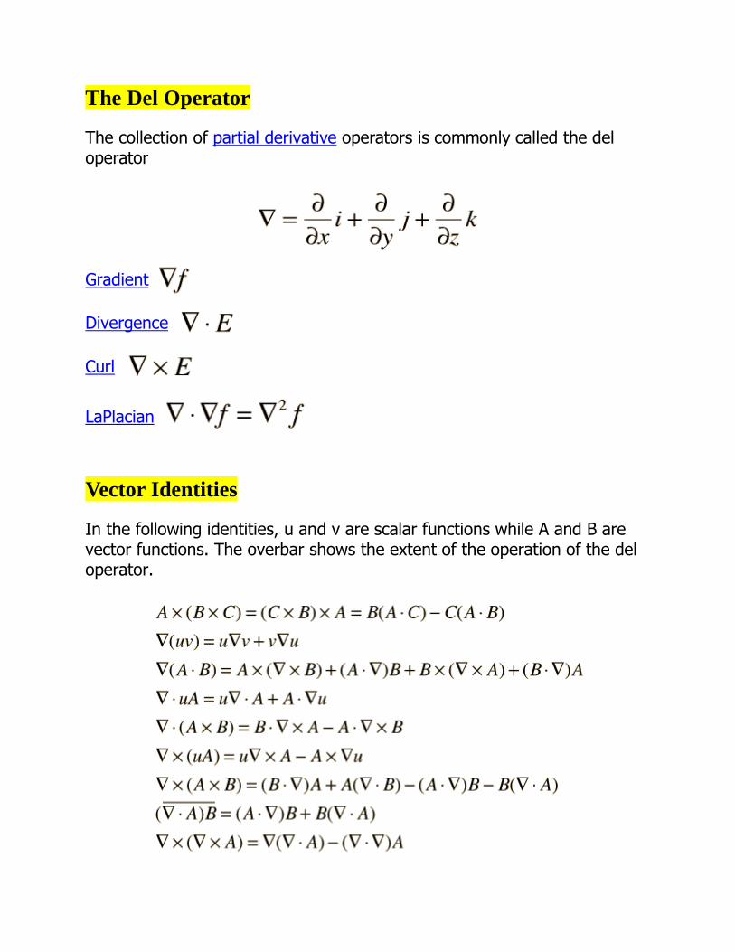
The Del Operator

The collection of partial derivative operators is commonly called the del operator

Gradient

Divergence

Curl

LaPlacian

Vector Identities

In the following identities, u and v are scalar functions while A and B are vector functions. The overbar shows the extent of the operation of the del operator.

Area Integral

An area integral of a vector function E can be defined as the integral on a surface of the scalar product of E with area element dA. The direction of the area element is defined to be perpendicular to the area at that point on the surface.

The outward directed surface integral over an entire closed surface is denoted

It is appropriate for such physical applications as Gauss' law.

Line Integral

Vector functions such as electric field and magnetic field occur in physical applications, and scalar products of these vector functions with another vector such as distance or path length appear with regularity. When such a product is summed over a path length where the magnitudes and directions change, that sum becomes an integral called a line integral.

LaPlace's and Poisson's Equations

A useful approach to the calculation of electric potentials is to relate that potential to the charge density which gives rise to it. The electric field is related to the charge density by the divergence relationship

and the electric field is related to the electric potential by a gradient relationship

Therefore the potential is related to the charge density by Poisson's equation

In a charge-free region of space, this becomes LaPlace's equation

This mathematical operation, the divergence of the gradient of a function, is called the LaPlacian. Expressing the LaPlacian in different coordinate systems to take advantage of the symmetry of a charge distribution helps in the solution for the electric potential V. For example, if the charge distribution has spherical symmetry, you use the LaPlacian in spherical polar coordinates. Since the potential is a scalar function, this approach has advantages over trying to calculate the electric field directly. Once the potential has been calculated, the electric field can be computed by taking the gradient of the potential.

Divergence Theorem

The volume integral of the divergence of a vector function is equal to the integral over the surface of the component normal to the surface.

Stokes' Theorem

The area integral of the curl of a vector function is equal to the line integral of the field around the boundary of the area.

The LaPlacian

The divergence of the gradient of a scalar function is called the Laplacian. In rectangular coordinates:

The Laplacian finds application in the Schrodinger equation in quantum mechanics. In electrostatics, it is a part of LaPlace's equation and Poisson's equation for relating electric potential to charge density.

Laplacian, Various Coordinates

Compared to the LaPlacian in rectangular coordinates:

In cylindrical polar coordinates:

and in spherical polar coordinates:

Relation of Electric Field to Charge Density

Since electric charge is the source of electric field, the electric field at any point in space can be mathematically related to the charges present. The simplest example is that of an isolated point charge. For multiple point charges, a vector sum of point charge fields is required. If we envision a continuous distribution of charge, then calculus is required and things can become very complex mathematically.

One approach to continuous charge distributions is to define electric flux and make use of Gauss' law to relate the electric field at a surface to the total charge enclosed within the surface. This involves integration of the flux over the surface.

Another approach is to relate derivatives of the electric field to the charge density. This approach can be considered to arise from one of Maxwell's equations and involves the vector calculus operation called the divergence. The divergence of the electric field at a point in space is equal to the charge density divided by the permittivity of space.

In a charge-free region of space wher

While these relationships could be used to calculate the electric field produced by a given charge distribution, the fact that E is a vector quantity increases the complexity of that calculation. It is often more practical to convert this relationship into one which relates the scalar electric potential to the charge density. This gives Poisson's equation and LaPlace's equation.

Electric Field from Voltage

One of the values of calculating the scalar electric potential (voltage) is that the electric field can be calculated from it. The component of electric field in any direction is the negative of rate of change of the potential in that direction.

If the differential voltage change is calculated along a direction ds, then it is seen to be equal to the electric field component in that direction times the distance ds.

The electric field can then be expressed as

This is called a partial derivative.

For rectangular coordinates, the components of the electric field are

Express as a gradient.

Electric Field as Gradient

The expression of electric field in terms of voltage can be expressed in the vector form

This collection of partial derivatives is called the gradient, and is represented by the symbol ∇ . The electric field can then be written

Expressions of the gradient in other coordinate systems are often convenient for taking advantage of the symmetry of a given physical problem.

Current Flow in Uniform Earth

As is the case for gravity and magnetics, we will find that electrical

potential, measured in Volts, has the same properties as gravity and

magnetic potentials, in that it is a scalar, and we can add the effects of

different sources of potential to find out where current will flow. Current will

flow in a direction normal to equipotential (equal voltage) surfaces.

Rather than have current flow only through wires, we will now plug our

wires into the earth and see how current flows through the earth, and how

to measure it to determine regions of anomalous resistivity.

Consider an electrode stuck in the ground with it's matching electrode far

away (just like a magnetic monopole). It's potential relative to the distant

electrode is measured in Volts.

Battery

current

current

equipotential

If we measure the potential difference between two shells at some a

distance D from the electrode, we get

dV iR i l

A

i

dr

2r 2

where dr is the thickness of the shell across which we measure the

potential, Recalling that the resistivity of air is so high, no current will flow

through it, so we only need have the surface of a hemisphere (2πr2

).

We now integrate in from infinity (where potential is zero) to get the

potential at a point a distance D from the source:

V dV i

2D

dr

r 2D

i

2D IF the resistivity of the ground is UNIFORM.

The current, i, above is the current IN THE WIRE, not the current in the

ground, which varies.

This is the basic equation of resistivity, in that we can add the potentials

from many sources to obtain a "potential" map of a surface. By contouring

that map, we have equipotential lines, along which no current flows.

Current flows in directions perpendicular to equipotential lines.

Sound familiar? It should! Magnetic lines of force are perpendicular to

magnetic equipotential surfaces, and the pull of gravity is perpendicular to

gravity equipotential surfaces.

TWO ELECTRODES: What if we move the other current electrode in from far away?

Battery

d

P1

zx

We can calculate the potential at point P1 by just adding the potentials from

both current electrodes - remembering that one is positive, and the other negative:

VP1

i

2r1

i

2r2

i

2

1

r1

1

r2

What is the potential between the electrodes vs. depth?

We just change the r values to x-z coordinates:

VP1

i

2

1

d2 x

2

z 2

1

d2 x

2

z 2

0

20

40

60

80

100

120

140

160

0

25

50

75

100

125

150

-350.0

-300.0

-250.0

-200.0

-150.0

-100.0

-50.0

0.0

potential

depth

distance from center

Potential at depth

We can’t measure the potential below the surface in the field, though. We’re

stuck at the surface. The surface potential looks like the profile below for a

current of 1 A, 100 m between electrodes, and a resistivity of 10km

Potential along surface

-400.0

-300.0

-200.0

-100.0

0.0

100.0

200.0

300.0

400.0

-200 -150 -100 -50 0 50 100 150 200

Distance

Po

ten

tial

If we put voltage probes at –65m and +65m along the x axis above,

what voltage would we see?

This allows us to contour equipotential lines, but how much current is

flowing in what areas? Current flows ALL THROUGH the subsurface, not

just directly from one electrode to the other. With some difficulty, it can be

shown that the fraction of the total current (if) flowing above a depth z for

an electrode separation d is given by:

if 2

tan1 2z

d

In a region of equal resistivity - about 70% of the current flows at depths

shallower than the distance between the electrodes.

With this information, we can sketch lines perpendicular to the

equipotentials that show where most of the current is flowing. Be careful,

though, this only works where the resistivity is constant throughout

the model! Note that all current lines are perpendicular to equipotential

lines - no current flows between two points where the potential is equal.

The most common form of resistivity measurement uses two current electrodes and two potential electrodes:

We use the same argument, summing potentials, to obtain the voltage

across two electrodes we get:

i

C1 P1 C2P2

r 2

r 4r 3

r 1

+ -

+ -

curren t

potentia l

The potential difference between P1 and P2 is:

VP1P2VP1

VP2

VP1 VC1

VC2

P1

, VP2 VC1

VC2

P2

VP1P2

i

2r1

i

2r2

i

2r3

i

2r4

i

2

1

r1

1

r2

1

r3

1

r4

Solving for the resistivity,:

2VP1 P2

i

1

1

r1

1

r2

1

r3

1

r4

Thus, we can measure the current, voltage, and appropriate distances and solve for resistivity.

In the example above we have current electrodes at ±50m, and voltage electrodes at ± 65m, so: r

1= 15m

r2= 115

r3= 115

r4= 15

and the current is 1.0 A

So we can solve for =(2 π*185 /1)*1/(1/15-1/115-1/115+1/15)= 1025.6 m.

Which is pretty close to the model value of 135 m.

BUT, this is a boring model; what we really want to know is what to expect

as the resistivity changes with depth.

CURRENT DENSITY AND FLOW LINES

If we think about current flow lines crossing the boundary between two

resistivities, it's almost like a seismic ray passing between two materials

with different velocities - but the formula is different:

tan1

tan 2

2

1

1.276

tan( 2)/tan( 1)=

y

y

2

1

0.111

Note that this is equivalent to z1/z

2=r

1/r

2, where z is the distance along

the vertical axis. So, if we make zi proportional to r

i then z

2 is proportional

to r2 , holding y constant, then we will get the current flow direction easily.

Note that he current flow lines get closer together when the current moves

into a region of lower reisistivity:

implying that the current density increases as we cross to the lower

resistivity material. If resistivity increases with depth, then current density

decreases. If resistivity in a region is VERY high ( insulator), then few flow

lines will cross a boundary with a conductor, and those that do will be

directed perpendicular to the boundary.

We can define the APPARENT RESISTIVITY as the resistivity we would get

assuming that no boundary or change in resistivity is present. So that

apparent resistivity equation is identical to the equation for a material with

constant resistivity:

a 2VP1P2

i

1

1

r1

1

r2

1

r3

1

r4

So, what does this tell us?

Recall that current density is qualitatively measured by the number of flow

lines. What is the relationship between potential difference V and current

density j ?

Since j=i/A, and i=V/R, and =RA/l, j=V/RA, or j=V/l. Thus,

current density is proportional to potential within a tube extending along the

flow line from the current electrode to the to the potential electrode. Does

this mean that if we measure high voltages we can expect high currents? !

? NO.

Consider measuring the potential between a wire and some point on the

outside of insulation around that wire. We would measure a high potential

difference between a point on the wire and a point outside the insulation -

does that mean that the current across the wire through the insulation will

be higher than the current through the wire?? !! What's wrong here?

The POTENTIAL difference is a function of the BATTERY - not the material.

So the higher the voltage of the battery, the higher the current density, but,

across an insulator, the current will be very low because the resistivity is

very high.

Variations in current density near the earth’s surface will be reflected in

changes in potential difference, and will result in changes in apparent

resistivity. Consider the cases below -

What happens if we move the layer up and down? If the interface is very

deep, RELATIVE TO THE ELECTRODE SPACINGS, the lower layer

should have no effect, and our readings shouldn't reflect its presence.

How deep is very deep?

What if we plot apparent resistivity vs. electrode spacing?

As spacing increases, we should "feel" deeper and deeper. At some point,

if our electrodes are far enough apart, the top layer will have considerably

less effect than the bottom

1> 2

a

elect rode spacing

Top layer bot t om layer

1< 2

This change in apparent resistivity with electrode spacing should give us the information we need to interpret data and determine the depth to an interface and the resistivity of the materials.

ELECTRODE CONFIGURATIONS

The value of the apparent resistivity depends on the geometry of the electrode

array used (K factor)

1- Wenner Arrangement

Named after wenner (1916) .

The four electrodes A , M , N , B are equally spaced along a straight line. The

distance between adjacent electrode is called “a” spacing . So AM=MN=NB=

⅓ AB = a.

Ρa= 2 π a V / I

The wenner array is widely used in the western Hemisphere. This array is

sensitive to horizontal variations.

2- Lee- Partitioning Array .

This array is the same as the wenner array, except that an additional potential

electrode O is placed at the center of the array between the Potential electrodes

M and N. Measurements of the potential difference are made between O and

M and between O and N .

Ρa= 4 π a V / I

This array has been used extensively in the past .

3) Schlumberger Arrangement .

This array is the most widely used in the electrical prospecting . Four electrodes

are placed along a straight line in the same order AMNB , but with AB ≥ 5 MN

MN

MNAB

I

Va

22

22

This array is less sensitive to lateral variations and faster to use as only

the current electrodes are moved.

1. Dipole – Dipole Array .

The use of the dipole-dipole arrays has become common since the 1950’s ,

Particularly in Russia. In a dipole-dipole, the distance between the current

electrode A and B (current dipole) and the distance between the potential

electrodes M and N (measuring dipole) are significantly smaller than the

distance r , between the centers of the two dipoles.

ρa = π [ ( r2 / a ) – r ] v/i

Or . if the separations a and b are equal and the distance between the centers

is (n+1) a then

ρa = n (n+1) (n+2) . π a. v/i

This array is used for deep penetration ≈ 1 km.

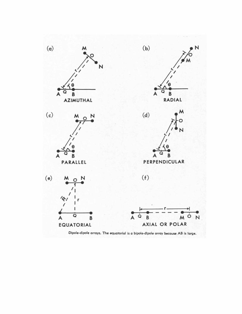
Four basic dipole- dipole arrays .

1) Azimuthal

2) Radial

3) Parallel

4) Perpendicular

When the azimuth angle (Ө ) formed by the line r and the current dipole AB = π /2

, The Azimuthal array and parallel array reduce to the equatorial Array.

When Ө = O , the parallel and radial arrays reduce to the polar or axial array .

If MN only is small is small with respect to R in the equatorial array, the system is

called Bipole-Dipole (AB is the bipole and MN is the dipole ), where AB is large

and MN is small.

If AB and MN are both small with respect to R , the system is dipole- dipole

5) Pole-Dipole Array .

The second current electrode is assumed to be a great distance from the

measurement location ( infinite electrode)

ρa = 2 π a n (n+1) v/i

6) Pole – Pole.

If one of the potential electrodes , N is also at a great distance.

Ρa= 2 π a V / I

Electrical Reflection Coefficient

Consider point current source and find expression for current potentials in medium

1 and medium 2: Use potential from point source, but 4π as shell is spherical:

Potential at point P in medium 1:

Potential at point Q in medium2:

At point on boundary mid-way between source and its image:

r1=r2=r3=r say. Setting Vp = Vq, and canceling we get:

k is electrical reflection coefficient and used in interpretation

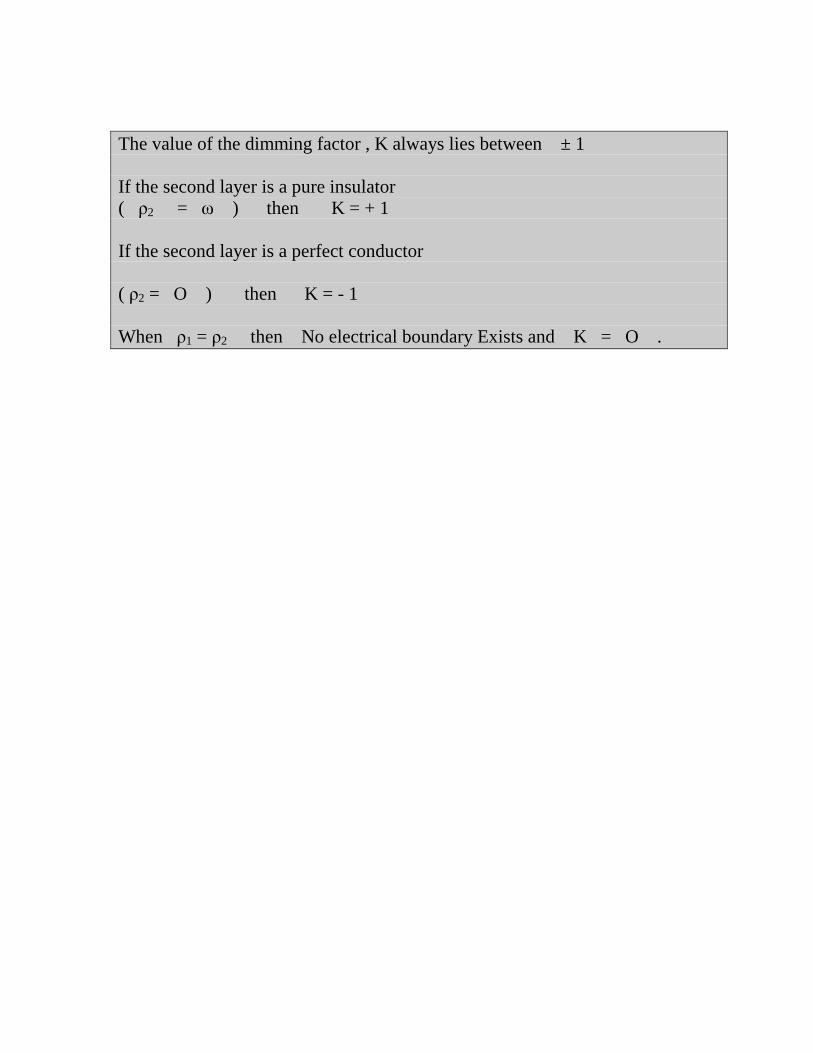
The value of the dimming factor , K always lies between ± 1

If the second layer is a pure insulator

( ρ2 = ω ) then K = + 1

If the second layer is a perfect conductor

( ρ2 = O ) then K = - 1

When ρ1 = ρ2 then No electrical boundary Exists and K = O .

SURVEY DESIGN

Two categories of field techniques exist for conventional resistivity analysis

of the subsurface. These techniques are vertical electric sounding (VES), and

Horizontal Electrical Profiling (HEP).

1- Vertical Electrical Sounding (VES) .

The object of VES is to deduce the variation of resistivity with depth below a

given point on the ground surface and to correlate it with the available

geological information in order to infer the depths and resistivities of the

layers present.

In VES, with wenner configuration, the array spacing “a” is increased by

steps, keeping the midpoint fixed (a = 2 , 6, 18, 54…….) .

In VES, with schlumberger, The potential electrodes are moved only

occasionally, and current electrode are systematically moved outwards in

steps

AB > 5 MN.

2- Horizontal Electrical profiling (HEP) .

The object of HEP is to detect lateral variations in the resistivity of the

ground, such as lithological changes, near- surface faults…… .

In the wenner procedurec of HEP , the four electrodes with a definite array

spacing “a” is moved as a whole in suitable steps, say 10-20 m. four

electrodes are moving after each measurement.

In the schlumberger method of HEP, the current electrodes remain fixed at

a relatively large distance, for instance, a few hundred meters , and the

potential electrode with a small constant separation (MN) are moved

between A and B .

Multiple Horizontal Interfaces

For Three layers resistivities in two interface case , four possible curve types

exist.

1- Q – type ρ1> ρ2> ρ3

2- H – Type ρ1> ρ2< ρ3

3- K – Type ρ1< ρ2> ρ3

4- A – Type ρ1< ρ2< ρ3

In four- Layer geoelectric sections, There are 8 possible relations :

ρ1> ρ2< ρ3< ρ4 HA Type

ρ1> ρ2< ρ3> ρ4 HK Type

ρ1< ρ2< ρ3< ρ4 AA Type

ρ1< ρ2< ρ3> ρ4 AK Type

ρ1< ρ2> ρ3< ρ4 KH Type

ρ1< ρ2> ρ3> ρ4 KQ Type

ρ1> ρ2> ρ3< ρ4 QH Type

ρ1> ρ2> ρ3> ρ4 QQ Type

Quantitative VES Interpretation: Master Curves

Layer resistivity values can be estimated by matching to a set of master curves

calculated assuming a layered Earth, in which layer thickness increases with depth.

(seems to work well). For two layers, master curves can be represented on a single

plot.

Master curves: log-log plot with ρa / ρ1 on vertical axis and a / h on

horizontal (h is depth to interface)

Plot smoothed field data on log-log graph transparency.

Overlay transparency on master curves keeping axes parallel.

Note electrode spacing on transparency at which (a / h=1) to get interface

depth.

Note electrode spacing on transparency at which (ρa / ρ1 =1) to get resistivity

of layer 1.

Read off value of k to calculate resistivity of layer 2 from:

Quantitative VES Interpretation: Inversion

Curve matching is also used for three layer models, but book of many more curves.

Recently, computer-based methods have become common:

forward modeling with layer thicknesses and resistivities provided by user

inversion methods where model parameters iteratively estimated from data

subject to user supplied constraints

Example (Barker, 1992)

Start with model of as many layers as data points and resistivity equal to measured

apparent resistivity value.

Calculated curve does not match data, but can be perturbed to improve fit.

Applications of Resistivity Techniques

1. Bedrock Depth Determination

Both VES and CST are useful in determining bedrock depth. Bedrock usually more

resistive than overburden. HEP profiling with Wenner array at 10 m spacing and 10

m station interval used to map bedrock highs.

2. Location of Permafrost

Permafrost represents significant difficulty to construction projects due to

excavation problems and thawing after construction.

Ice has high resistivity of 1-120 ohm-m

3. Landfill Mapping

Resistivity increasingly used to investigate landfills:

Leachates often conductive due to dissolved salts

Landfills can be resistive or conductive, depends on contents

Limitations of Resistivity Interpretation

1- Principle of Equivalence.

If we consider three-lager curves of K (ρ1< ρ2> ρ3 ) or Q type (ρ1> ρ2> ρ3)

we find the possible range of values for the product T2= ρ2 h2 Turns out to

be much smaller. This is called T-equivalence. H = thickness, T :

Transverse resistance it implies that we can determine T2 more reliably

than ρ2 and h2 separately. If we can estimate either ρ2 or h2 independently

we can narrow the ambiguity. Equivalence: several models produce the

same results. Ambiguity in physics of 1D interpretation such that

different layered models basically yield the same response.

Different Scenarios: Conductive layers between two resistors, where

lateral conductance (σh) is the same. Resistive layer between two

conductors with same transverse resistance (ρh).

2- Principle of Suppression.

This states that a thin layer may sometimes not be detectable on the field

graph within the errors of field measurements. The thin layer will then be

averaged into on overlying or underlying layer in the interpretation. Thin

layers of small resistivity contrast with respect to background will be missed.

Thin layers of greater resistivity contrast will be detectable, but equivalence

limits resolution of boundary depths, etc.

The detectibility of a layer of given resistivity depends on its relative

thickness which is defined as the ratio of Thickness/Depth.

Comparison of Wenner and Schlumberger

(1) In Sch. MN ≤ 1/5 AB

Wenner MN = 1/3 AB

(2) In Sch. Sounding, MN are moved only occasionally.

In Wenner Soundings, MN and AB are moved after each measurement.

(3) The manpower and time required for making Schlumberger soundings are

less than that required for Wenner soundings.

(4) Stray currents that are measured with long spreads effect

measurements with Wenner more easily than Sch.

(5) The effect of lateral variations in resistivity are recognized and corrected

more easily on Schlumberger than Wenner.

(6) Sch. Sounding is discontinuous resulting from enlarging MN.

Disadvantages of Wenner Array

1. All electrodes must be moved for each reading

2. Required more field time

3. More sensitive to local and near surface lateral variations

4. Interpretations are limited to simple, horizontally layered structures

Advantages of Schlumberger Array

1. Less sensitive to lateral variations in resistivity

2. Slightly faster in field operation

3. Small corrections to the field data

Disadvantages of Schlumberger Array

1. Interpretations are limited to simple, horizontally layered structures

2. For large current electrodes spacing, very sensitive voltmeters are required.

Advantages of Resistivity Methods

1. Flexible

2. Relatively rapid. Field time increases with depth

3. Minimal field expenses other than personnel

4. Equipment is light and portable

5. Qualitative interpretation is straightforward

6. Respond to different material properties than do seismic and other methods,

specifically to the water content and water salinity

Disadvantages of Resistivity Methods

1- Interpretations are ambiguous, consequently, independent geophysical

and geological controls are necessary to discriminate between valid

alternative interpretation of the resistivity data ( Principles of Suppression

& Equivalence)

2- Interpretation is limited to simple structural configurations.

3- Topography and the effects of near surface resistivity variations can mask

the effects of deeper variations.

4- The depth of penetration of the method is limited by the maximum

electrical power that can be introduced into the ground and by the

practical difficulties of laying out long length of cable. The practical

depth limit of most surveys is about 1 Km.

5. Accuracy of depth determination is substantially lower than with

seismic methods or with drilling.

Lateral inhomogeneities in the ground affect resistivity measurements in

different ways: The effect depends on

The size of inhomogeneity with respect to its depth

2. The size of inhomogeneities with respect to the size of electrode array

3. The resistivity contrast between the inhomogeneity and the surrounding

media

4. The type of electrode array used

5. The geometric form of the inhomogeneity

6. The orientation of the electrode array with respect to the strike of the

inhomogeneity

Mise-A-LA-Masse Method

This is a charged-body potential method is a development of HEP technique

but involves placing one current electrode within a conducting body and the

other current electrode at a semi- infinite distance away on the surface .

This method is useful in checking whether a particular conductive mineral-

show forms an isolated mass or is part of a larger electrically connected ore

body.

There are two approaches in interpretation

1- One uses the potential only and uses the maximum values a being

indicative of the conductive body.

2- The other converts the potential data to apparent resistivity and thus a

high surface voltage manifests itself in a high apparent resistivity

ρa = 4Л X V/I :

Where X is the distance between C1 and P1.

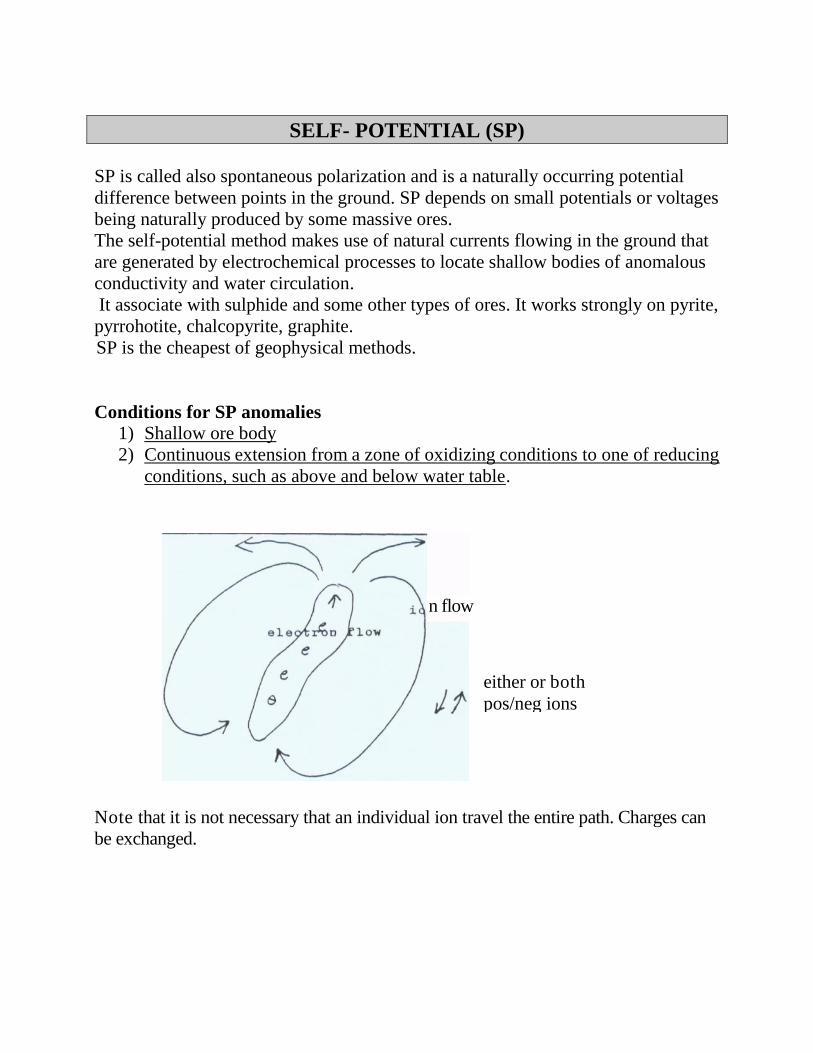
SELF- POTENTIAL (SP)

SP is called also spontaneous polarization and is a naturally occurring potential

difference between points in the ground. SP depends on small potentials or voltages

being naturally produced by some massive ores. The self-potential method makes use of natural currents flowing in the ground that

are generated by electrochemical processes to locate shallow bodies of anomalous

conductivity and water circulation.

It associate with sulphide and some other types of ores. It works strongly on pyrite,

pyrrohotite, chalcopyrite, graphite.

SP is the cheapest of geophysical methods.

Conditions for SP anomalies

1) Shallow ore body

2) Continuous extension from a zone of oxidizing conditions to one of reducing

conditions, such as above and below water table.

Note that it is not necessary that an individual ion travel the entire path. Charges can

be exchanged.

n flow

either or both

pos/neg ions

The implications of this for potential distribution would be

When we come to consider more specifically the mechanism, we see that it must

be consistent with

- electron flow in the ore body

- ion flow in surrounding rock

- no transfer of ions across ore boundary, although electrons are free to cross

That is we must have

negative ion

neutral ion

positive ion

neutral ion

reverse process

When we consider the possible ion species, the criteria would be

- common enough

- reversible couple under normal ground conditions

- mobile enough

Sato and Mooney proposed ferric/ferrous couples to satisfy these criteria.

made continuous by reactions

involving ferrous and ferric

hydroxide with presence of H+

made continuous by O2 – H2 O2

reaction with O2 supplied

from atmosphere

Proposed electrochemical mechanism for self-potentials

This proposed mechanism have two geologic implications:

1) The ore body must be an electronic conductor with high conductivity.

This would seem to eliminate sphalerite (zinc sulfide) which has low

conductivity.

2) The ore body must be electrically continuous between a region of oxidizing

conditions and a region of reducing conditions. While water table contact

would not be the only possibility have, it would seem to be a favorable one.

Instrumentation and Field Procedure

Since we wish to detect currents, a natural approach is to measure current.

However, the process of measurement alters the current. Therefore, we arrive at

it though measuring potentials.

Principle, and occasional practice:

More usual practice

Instruments

Equipment:

- potentiometer or high impedance voltmeter

- 2 non-polarizing electrodes

- wire and reel

Non-polarizing electrodes were described in connection with resistivity exploration although

they are not usually required there. Here, they are essential. The use of simple metal

electrodes would generate huge contact or corrosion potentials which would mask the

desired effect. non-polarizing electrodes consist of a metal in contact with a saturated

solution of a salt of the metal . Contact with the earth can be made through a porous

ceramic pot.

The instrument which measures potential difference between the electrodes must have the

following characteristics:

a) capable of measuring +0.1 millivolt,

b) capable of measuring up to ±1000 millivolts (±1 volt)

c) input impedance greater than 10 megaohms, preferably more.

The high input impedance is required in order to avoid drawing current through the

electrodes, whose resistance is usually less than 100 kilohms. In very dry conditions (dry

rock, ice, snow, frozen soil), the electrode resistance may exceed 100 kilohms, in which case

the instrument input impedance should also be increased.

SP are produced by a number of mechanisms :

1) Mineral potential (ores that conduct electronically ) such as most sulphide ores

,Not sphalerite (zinc sulphide) magnetite, graphite. Potential anomaly over sulfide

or graphite body is negative The ore body being a good conductor. Curries current

from oxidizing electrolytes above water – table to reducing one below it .

2) Diffusion potential

Ed == = Ln (C1 / C2 )

Where

Ia , Ic Mobilities of the anions (+ve) and cations( -ve )

R= universal Gas constant ( 8.314JK-1 mol-1 )

T : absolute temperature ( K)

N : is ionic valence

F: Farady’s constant 96487 C mol-1 )

C1 , C2 Solution concentrations .

RT( Ia – Ic)

n F(Ia+Ic)

3) Nernst Potential

EN = - ( RT / nF ) Ln ( C1 / C2 )

Where Ia = Ic in the diffusion potential Equation .

4. Streaming potentials due to subsurface water flow are the source of many SP

anomalies. The potential E per unit of pressure drop P (The streaming potentials

coupling cocfficent) is given by :

EK =

ρ Electrical Resistivity of the pore Fluld.

Ek Electro-kinetic potential as a result from an electrolyte flowing through a

porous media.

ε Dielectric constant of the pole fluid.

η Viscosity of the pore fluid

δP pressure difference

CE electro filtration coupling coefficient.

If the grain size decreases, C increases

• If the temperature decreases, C decreases

• If viscosity decreases, C increases

• Permeability has a complex effect on C

.

ε ρ CE δP

4 π η

Advantages :

Survey simple

Non expensive

Allows for a rapid qualitative mapping of the underground

Suitable for monitoring

Disadvantages

Very sensitive to noise

• Physical aspects still not well understood

• Quantitative aspects still need to be develop

Interpretation

Usually, interpretation consists of looking for anomalies.

The order of magnitude of anomalies is

0-20 mv normal variation

20-50 mv possibly of interest, especially if observed over a fairly large area

over 50 mv definite anomaly

400-1000 mv very large anomalies

Depth of investigation depends on the size of the mineralized body and the depth of

the water table for a mineralization potential (generally shallow, < 30 m)

• Interpretation mainly qualitative (profile, map)

• Quantitative using dipole approximations for the polarized

body (similar to magnetic interpretation)

Applications

Groundwater applications rely principally upon potential differences produced by

pressure gradients in the groundwater. Applications have included

detection of leaks in dams and reservoirs

location of faults, voids, and rubble zones which affect groundwater flow

delineation of water flow patterns around landslides, wells, drainage structures, and

springs, studies of regional groundwater flow

Other groundwater applications rely upon potential differences produced by

gradients in chemical concentration, Applications have included

outline hazardous waste contaminant plumes

Thermal applications rely upon potential differences produced by temperature

gradients.

Applications have included

geothermal prospecting

map burn zones for coal mine fires

monitor high-temperature areas of in-situ coal gasification processes and oil field

steam and fire floods.

Induced Polarization ( IP)

IP depends on a small amount of electric charge being stored in an ore when a

current is passed Through it , to be released and measured when the current is

switched off .

The main application is in the search for disseminated metallic ores and to a

lesser extent, ground water and geothermal exploration .

Measurements of IP using 2 current electrodes and 2 non-polarizable potential

electrodes. When the current is switched off , the voltage between the potential

electrodes takes a finite to decay to zero because the ground temporarily stores

charge ( become Polarized)

Four systems of IP .

1- Time domain

2- Frequency domain < 10 HZ

3- Phase domain

4- Spectral IP 10-3 to 4000 HZ

Sources of IP Effects

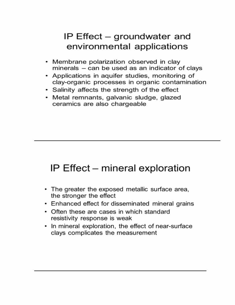
1) Normal IP

Membrane Polarization

Most Pronounced with clays

Decreases with very high (> 10%) clay content due to few pores, low

conductivity.

2) Electrode polarization

Most metallic minerals have EP

Decreases with increased porosity.

Over-voltage effect

3) IP is A bulk effect.

Grain (electrode) polarization. (A) Unrestricted electrolytic flow in an open channel.

(B) Polarization of an electronically conductive grain, blocking a channel

t2

1. Time – domain measurements.

One measure of the IP effects is the ratio Vp / Vo which is known chargeability

which expressed in terms of millivolts per volt or percent.

Vp : overvoltage

Vo : observed voltage

M= Vp / Vo ( mv /v or %)

Apparent chargeability

Ma = ( 1 / V0 ) ∫t1 Vp (t) dt = A / V0

Vp ( t) is the over-voltage at time t .

10 – 20 % sulphides 1000-3000 msec .

Sand stones 100-200 msec.

Shale 50-100

Water 0

2) Frequency- Domain measurements.

Frequency effect FE= (Pao –Pa1) / Pa1 ( unitless )

Pao : apparent resistivity at low frequencies

Pal : appatent resistivity at high frequencies

Pao > Pa1

Percentage frequency affect PFE = 100(Pao –Pa1) / Pa1 = 100 FE

The frequency effect in the frequency domain is equivalent to the

chargeability in the time domain for a weakly polarisable medium where FE

< 1 .

Metal Factor MF= A (ρa0 – ρa1) / (ρa0 ρa1)

= A ( δa1 – δa0 ) siemens / m

ρa0 & ρa1 apparent resistivity.

δa0 and δa1 are apparent conductivities (1/ ρa ) at low and higher frequencies

respectively where

ρa0 > ρa1 and δa0 < δa1 A = 2 π x 105

MF = A x FE / ρa0 = A x FE / ρa0

= FE / ρa0 = A x FE x δa0

The above methods do not give a good indication of the relative amount of the

metallic mineralization within the source of the IP. It is necessary to go with

spectral IP.

3. Spectral IP and Complex Resistivity.

Is the measurement of the dielectric properties of materials

Ө is the phase lag between the applied current and the polarization voltage

measured.

| z(w) | = P0 [ 1 – M ( 1 – 1/ ( 1+(iwτ)c ) ]

Z(w) : complex resistivity

P0 : D.c. resistivity

M : IP chargeability

W : Angular frequency.

τ : Time constant. (relaxation time) is the behaviour between the lower

and upper frequency limits.

i : √ -1

c : frequency exponent

Critical Frequency (Fc) : Which is the specific frequency at which the

maximum phase shift is measured. This frequency is completely independent of

resistivity.

Phase angle and the critical frequency increase with increasing chargeability.

Fc = [ 2 π τ ( 1 – M)1/2c ]-1

τ Time constant

M IP chargeability .

This is call cole – cole relalaxation

IP Survey Design

1- Profiling : Later contrasts in electrical properties such as lithologic

contacts. (wenner + Dipole – Dipole) .

2- Sounding : to map the depths and thickness of stratigraphic units

(Schlumberger + wenner).

3- Profiling – Sounding : in contaminant plume mapping , where subsurfae

electrical propertios are expected to vary vertically and horizontally (wenner

+ Dipole – Dipole) .

Limitations of IP

1- IP is more susceptible to sources of cultural interference (metal

fences, pipe lines , power lines) than electrical resistivity.

2- IP equipment requires more power than resistivity alone . This translates

into heavier field instruments

3- The cost of IP much greater than resistivity – alone system.

4- IP requires experience.

5- Complexity in data interpretation.

6- Intensive field work requires more than 3 crew members.

7- IP requires a fairly large area far removed from power lines , fences,

pipelines .

Advantages of IP

1- IP data can be collected during an electrical resistivity survey

2- IP data and resistivity together improves the resolution of the analysis of

Resistivity data in three ways:

a. some of the ambiguities in resistivity data can be redueed by IP

analysis.

b. IP can be used to distinguish geologic layers which do not respond

well to an electrical resistivity .

c. Measurements of chargeability can be used to discriminate equally

electrically conductive target such as saline, electrolytic or metallic-

ion contaminant plumes from clay Layers.

ELECTROMAGNETIC METHODS

Introduction

Electromagnetic methods in geophysics are distinguished by:

1. Use of differing frequencies as a means of probing the Earth (and other planets),

more so than source-receiver separation. Think “skin depth”. Sometimes the

techniques are carried out in the frequency domain, using the spectrum of natural

frequencies or, with a controlled source, several fixed frequencies (FDEM method -

--“frequency domain electromagnetic”). Sometimes the wonders of Fourier theory

are involved and a single transient signal (such as a step function) containing, of

course, many frequencies, is employed (TDEM method - “time domain

electromagnetic”). The latter technique has become very popular.

2. Operate in a low frequency range, where conduction currents predominate over

displacement currents. The opposite is true (i.e., has to be true for the method to

work) in Ground Penetrating Radar (GPR). GPR is a wave propagation

phenomenon most easily understood in terms of geometrical optics. Low frequency

EM solves the diffusion equation.

3. Relies on both controlled sources (transmitter as part of instrumentation) and

uncontrolled sources. Mostly the latter is supplied by nature, but also can be

supplied by the Department of Defense.

EM does not require direct Contact with the ground. So, the speed with EM can

be made is much greater than electrical methods.

EM can be used from aircraft and ships as well as down boreholes.

Advantages

lightweight & easily portable.

Measurement can be collected rapidly with a minimum number of

field personnel .

Accurate

Good for groundwater pollution investigations.

Limitations :

Cultural Noise

Applications

1. Mineral Exploration

2. Mineral Resource Evaluation

3. Ground water Surveys

4. Mapping Contaminant Plumes

5. Geothermal Resource investigation

6. Contaminated Land Mapping

7. Landfill surveys

8. Detection of Natural and Artificial Cavities

9. Location of geological faults

10. Geological Mapping

Type of EM Systems

- EM can be classified as either :

1. Time – Domain (TEM) or

2. Frequency- Domain (FEM)

- FEM use either one or more frequencies.

- TEM makes measurements as a function of time .

- EM can be either :

a- Passive, utilizing natural ground signals (magnetotellurics)

b- Active , where an artificial transmitter is used either in the near-field (As in

ground conductivity meters) or in the far-field (using remote high-powered

military transmitters as in the case of VLF Mapping 15-24 KHZ ).

Factors Affecting EM Signal

The signal at the Receiver depends on :

1) the material 2) Shape 3) Depth of the Target

4) Design and positions of the transmitter and receiver coils .

The size of the current induced in the target by the transmitter depends on

1) Number of lines of magnetic field through the Loop (magnetic flux ) 2) Rate of

change of this number 3) The material of the loop.

Magnetic flux Depends on :

1) The Strength of the magnetic field at the Loop 2) Area of the Loop 3)

Angle of the loop to the field

Flux Ø = Magnetic field X cos Ө X area X number of turns .

Principle of EM surveying

- EM field can be generated by passing an alternating current through either a

small coil comprising many turns of wire or a large loop of wire .

- The frequency range of EM radiation is very wide, from < 15 HZ ( atmospheric

micropulsations) , Through radar bands (108 – 1011 HZ) up to X-ray and gamma

>1016 HZ .

- For geophysical Applications less than few thousand hertz, the wavelength of

order 15-100 km , typical source- receiver separation is much smaller ( 4-10 m )

The primary EM field travels from the transmitter coil to the receiver coil via paths

both above and below the surface.

In the presence of conducting body, the magnetic component of the EM field

penetrating the ground induces alternating currents or eddy currents to flow in the

conductor.

The eddy currents generate their own secondary EM field which travels to the

receiver. Differences between TX and RX fields reveal the presence of the

conductor and provide information on its geometry and electrical properties.

Depth of Penetration of EM

Skin Depth : is the depth at which the amplitude of a plane wave has decreased to

1/e or 37% relative to its initial amplitude Ao .

Amplitude decreasing with depth due to absorption at two frequencies

Az = Ao e-1

The skin depth S in meters = √ 2 / ωσ μ = 503 √ f σ

ω = 2π f = 503 √ ρ / f = 503 √ρ λ / v

σ : conductivity in s/m

μ : magnetic permeability (usually ≈ 1)

λ : wavelength , f : frequency , v : velocity , p : Resistivity thus, the

depth increases as both frequency of EM field and conductivity decrease.

Ex. In dry glacial clays with conductivity 5x 10-4 sm-1 , S is about 225 m at a

frequency of 10 KHZ .

Skin depths are shallower for both higher frequencies and higher conductivities

(Lower resistivities ).

Magnetotelluric Methods ( MT )

Telluric methods: Faraday's Law of Induction: changing magnetic fields

produce alternating currents. Changes in the Earth's magnetic field produce

alternating electric currents just below the Earth's surface called Telluric currents.

The lower the frequency of the current, the greater the depth of penetration.

Telluric methods use these natural currents to detect resistivity differences which

are then interpreted using procedures similar to resistivity methods.

MT uses measurements of both electric and magnetic components of The Natural

Time-Variant Fields generated.

Major advantages of MT is its unique Capability for exploration to very great

depths (hundreds of kilometers) as well as in shallow Investigations without using

of an artificial power source .

Natural – Source MT uses the frequency range 10-3-10 HZ , while audio –

frequency MT (AMT or AFMAG) operates within 10-104 HZ .

The main Application of MT in hydrocarbon Expl. and recently in meteoric impact,

Environmental and geotechnical Applications.

Pa = 0.2 / f │Ex / By │2 = 0.2 / f │Ex / Hy │2 = 0.2 / f │Z│2

Ex (nv/km) , By , orthogonal electric and magnetic components.

By : magnetic flux density in nT .

Hy : magnetizing force (A/m) .

Z : cagniard impedance.

The changing magnetic fields of the Earth and the telluric currents they produce

have different amplitudes. The ratio of the amplitudes can be used to determine the

apparent resistivity to the greatest depth in the Earth to which energy of that

frequency penetrates.

Typical equation:

apparent resistivity =

where Ex is the strength of the electric field in the x direction in millivolts

Hy is the strength of the magnetic field in the y direction in gammas

f is the frequency of the currents

Depth of penetration =

This methods is commonly used in determining the thickness of sedimentary

basins. Depths are in kilometers

Field Procedure

MT Comprises two orthogonal electric dipoles to measure the two horizontal

electric components and two magnetic sensors parallel to the electric dipoles to

measure the corresponding magnetic components .

1. Two orthogonal grounded dipoles to measure electric components

2. Three orthogonal magnetic sensors to measure magnetic components.

Thus, at each location, five parameters are measured simultaneously as a function

of frequency. By measuring the changes in magnetic (H) and electric (E) fields

over a range of frequencies an apparent resistivity curve can be produced. The

lower the frequency, the grater is the depth penetration.

Survey Design

EM data can be acquired in two configurations

1) Rectangular grid pattern

2) Along a traverse or profile .

EM equipment Operates in frequency domain. It allows measurement of both the .

1) in-phase (or real ) component .

2) 900 out – of – phase (or quadrature ) component.

Very Low Frequency (VLF) Method

VLF : uses navigation signal as Transmitter .

Measures tilt & phase

Main field is horizontal .

VLF detects electrical conductors by utilizing radio signal in the 15 to 30 KHZ

range that are used for military communications.

VLF is useful for detecting long, straight electrical conductors

VLF compares the magnetic field of the primary signal (Transmitted ) to that of

the secondary signal ( induced current flow with in the subsurface electrical

conductor).

Advantages of VLF

1) Very effective for locating zones of high electrical conductivity

2) fast

3) inexpensive

4) Requires one or two people .

Tilt Angle Method

Tilt angle systems have no reference link between Tx and Rx coils . Rx measures

the total field irrespective of phase and the receiver coil tilted to direction of

maximum or minimum magnetic field strength .

The response parameter of a conductor is defined are the product of conductivity –

thickness ( T) , permeability (μ ) an angular frequency

ω = 2π f and the square of the target a2 .

Poor conductors have response parameter < 1

Excellent conductor have response parameter greater than 1000

A Good conductor having a higher ratio AR / Ai

AR : Amplitude of Read (in – phase )

Ai : Amplitude of imaginary ( out – of phase)

In the left side of the above figure and poor conductor having a lower ratio of AR/

Ai .

Slingram System

slingram is limited in the size of TX coil. This system has the Transmitter and

Receiver connected by a cable and their separation kept constant as they are

moved together along a traverse.

Magnetic field Through The receiver has two sources :

a) The primary field of The Transmitter .

b) The secondary field produced by The Target .

Turam system

More powerful system than Slingram. It uses a very large stationary Transmitter

coil or wire laid out on the ground, and only The receiver is moved . TX 1-2 km

long, loop over 10 km long. The receiver consists of two coils and kept a fixed

distance between 10-50 m apart.

Ground Surveys of EM

A. Amplitude measurement

1- Long wire

Receiver pick up horizontal component of field parallel to wire .

Distortions of Normal field pattern are related to changes in

subsurface conductivity.

B. Dip-Angle

Measures combined effect of primary and secondary fields at the receiver.

AFMAG : Dip-angle method that uses Naturally occurring ELF signals

generated by Thunder storms.

Phase Component Methods

1) Work by comparing secondary & primary fields .

2) Compensator & Turam (long wire) .

3) Slingram Moving Trans / receiver

- Penetration ≈ ½ spacing of coil .

- Coil spacing critical .

Over barren ground Null is at zero coil dip-Angle.

Near conductor, dip angle ≠ 0

Dip – Angle is zero over Narrow conductor, and changes sign.

Dip-Angle method

1) easy , cheap

2) Quick

3) Sensitive to vertical

4) Difficult to distinguish between depth & conductivity

TDEM Method

A significant problem with many EM surveying techniques is that a small

secondary field must be measured in the presence of a much larger primary field,

with a consequent decrease in accuracy. This is circumvented to some extent in the

FDEM method described about by measuring the out-of-phase component.

In a TDEM approach, the signal is not a continuous frequency but instead consists

by a series of step-like pulses separated by periods where there is no signal

generated, but the decay of the secondary field from the ground is measured. The

induction

currents induced in a subsurface conductor diffuse outward when the inducing

energy is suddenly switched off. The measurement of the field at a number of time

steps is equivalent of measuring at several frequencies in an FDEM system.

Usually two-coil systems are used and the results can be stacked to reduce noise.

Modeling of the decay for layered systems, and more complicated conductivity

geometry, can be carried out.

The figure above shows the behavior of the field for two different conductivities. If

samples at different times were taken, then on could distinguish between the two

conductivities. This is the principle of Time Domain Electromagnetic (TDEM)

methods.

τ = σ μ L2 = σ μ A

where τ is a characteristic time constant and L and A correspond to a characteristic

length scale and characteristic area, respectively.

The EM61 has a single time sample at t 0.5 ms. Using a cylinder of radius 2 cm

and a conductivity of steel of 107 S m-1, then exp(-t/ τ ) = 0.56. where t is time

constant.

On the other hand, assume a plastic drum of seawater of conductivity 10 S m-1 and

radius 40 cm, then we obtain exp(-t/ τ ) = 0.

Airborne Electromagnetic Surveys

The general objective of AEM (Airborne ElectroMagnetic) surveys is to conduct a

rapid and relatively low-cost search for metallic conductors, e.g. massive sulphides,

located in bed-rock and often under a cover of overburden and/or fresh water. This

method can be applied in most geological environments except where the country

rock is highly conductive or where overburden is both thick and conductive. It is

equally well suited and applied to general geologic mapping, as well as to a variety

of engineering problems (e.g., fresh water exploration.) Semi-arid areas,

particularly with internal drainage, are usually poor AEM environments.

Conductivities of geological materials range over seven orders of magnitude, with

the strongest EM responses coming from massive sulphides, followed in decreasing

order of intensity by graphite, unconsolidated sediments (clay, tills, and

gravel/sand), and igneous and metamorphic rocks. Consolidated sedimentary rocks

can range in conductivity from the level of graphite (e.g. shales) down to less than

the most resistive igneous materials (e.g. dolomites and limestones). Fresh water is

highly resistive. However, when contaminated by decay material, such lake bottom

sediments, swamps, etc., it may display conductivity roughly equivalent to clay and

salt water to graphite and sulphides.

Typically, graphite, pyrite and or pyrrhotite are responsible for the observed

bedrock AEM responses. The following examples suggest possible target types and

we have indicate the grade of the AEM response that can be expected from these

targets.

Massive volcano-sedimentary stratabound sulphide ores of Cu, Pb, Zn, (and

precious metals), usually with pyrite and/or pyrrhotite. Fair to good AEM

targets accounting for the majority of AEM surveys.

Carbonate-hosted Pb-Zn, often with marcasite, pyrite, or pyrrhotite, and

sometimes associated with graphitic horizons. Fair to poor AEM targets.

Massive pyrrhotite-pentlandite bodies containing Ni and sometimes Cu and

precious metals associated with noritic or other mafic/ultramafic intrusive

rocks. Fair to good AEM targets.

Vein deposits of Ag, often with Sb, Cu, Co, Ni, and pyrite in volcanic and

sedimentary rocks. Generally poor AEM targets.

Quartz veins containing Au with pyrite, sometimes also with Sb, Ag, Bi, etc.,

in volcanic or sedimentary (and possibly intrusive) rocks. Poor AEM targets.

Basic Principles of Airborne

Electromagnetic-induction prospecting methods, both airborne and (most) ground

techniques, make use of man-made primary electromagnetic fields in, roughly, the

following way: An alternating magnetic field is established by passing a current

through a coil, (or along a long wire). The field is measured with a receiver

consisting of a sensitive electronic amplifier and meter or potentiometer bridge.

The frequency of the alternating current is chosen such that an insignificant eddy-

current field is induced in the ground if it has an average electrical conductivity,

If the source and receiver are brought near a more conductive zone, stronger eddy

currents may be caused to circulate within it and an appreciable secondary

magnetic field will thereby be created. Close to the conductor, this secondary or

anomalous field may be compared in magnitude to the primary or normal field

(which prevails in the absence of conductors), in which case it can be detected by

the receiver. The secondary field strength, Hs, is usually measured as a proportion

of the primary field strength, Hp, at the receiver in percent or ppm (parts per

million).

Anomaly = Hs / Hp.

Increasing the primary field strength increases the secondary field strength

proportionally but the "anomaly" measured in ppm or percent remains the same.

prospecting for anomalous zones is carried out by systematically traversing the

ground either with the receiver alone or with the source and receiver in

combination, depending on the system in use. In the case of airborne systems, the

receiver coils are usually in a towed bird and the transmitter may be a large coil

encircling a fixed wing aircraft, e.g. INPUT systems, or one or more small coils in

the same bird that houses the transmitting coils, e.g. most HEM (Helicopter EM)

systems.

There are two different basic systems commonly used to generate and receive the

electromagnetic field: transient or "time domain" systems like INPUT,GEOTEM

and MEGATEM and a/c. "frequency domain" systems like most HEM systems.

Transient Airborne Electromagnetics

Historically, the most commonly encountered system of this type was the INPUT

system. The newer systems GEOTEM and MEGATEM (Fugro Airborne Surveys)

function in a similar way to INPUT

In the INPUT system the transmitting coil, usually encircling a fixed wing aircraft,

is energized by what is, essentially, a step current. In the absence of conductors, a

sharp transient pulse proportional to the time derivative of the magnetic field is

induced in the receiver. When a conductor is present, however, a sudden change in

magnetic field intensity will induce in it a flow of current in the conductor which

will tend to slow the decay of the field.

The receiver "listens" only while the transmitter is "quiet" so that problems arising

out of relative motion between transmitter and receiver, because the receiver is

towed in a bird behind the aircraft, are virtually eliminated. Moreover, if the entire

decay of the secondary field could be observed, the response would be equivalent

to AC measurements made over the whole of the frequency spectrum. It is

important to note in this connection, however, that not the decay function itself but

only its time derivative can be recorded if a coil is used as the detector. This means

that the anomalous fields which decay very slowly are suppressed in amplitude

more than the others, and since these are the very ones generally associated with

good conductors, there would seem to be an inherent weakness in this system.

Because it is difficult to precisely synchronize the instant when the transmitter

becomes "quiet" with the instant that the receiver begins to "listen", it is nearly

impossible to record the entire function. This is equivalent to being unable to

record many of the lower frequencies in the a-c spectrum.

Typically, the time derivative of the decay function is measured using from six to

twelve different time delays from the instant that transmitter stops transmitting

before recording the signal received.

A sketch of the INPUT transient airborne EM system operation. The primary field

is a step function and the receiver records the decay of the field after the transmitter

stops transmitting. (Grant and West 1965)

Frequency Domain Airborne Electromagnetics

In the typical frequency domain helicopter EM system (HEM) both the transmitting

coil set and the receiver coil set are housed in a rigid boom or "bird" that is towed

beneath the helicopter. Commonly, this boom is from three to five meters long and

contains from two to six coil pairs. Usually, half of the coils in each of the

transmitter set and the receiver set are "co-axial", i.e. an axis normal to the plane of

the coils passes through the centre of both coils. The second half of the coil sets are

normally "co-planar", being equivalent to both the transmitting and receiving coil

lying flat on the ground. Other coplanar orientations have been used occasionally.

The receiver measures the in-phase and out-of-phase, or quadrature, of the

secondary field, expressed in ppm of the primary field. The two different coil

orientations provide data that is useful in discriminating between dike like

conductors that have considerable vertical extent and may be ore bodies, and

horizontal sheet like conductors that are simply conductive overburden.

Factors Affecting Detectability

1. Signal-to-noise ratio:

In practice, because of "system noise" (Ns) and "geological noise" (Ng), the ability

of a system to recognize and measure an anomaly is limited by the "signal-to-

noise" ratio: Signal-to-noise = Hs / (Ns + Ng)

Because Hs and Ng are proportional to the primary field strength Hp, and Ns, in

frequency-domain systems, usually contains elements proportional to Hp, there is

little to be gained by increasing the primary field power. In time domain systems

Ns is not greatly affected by Hp, so extra power does result in increased signal-to-

noise. Attempts to increase the signal-to-noise are sometimes made by increasing

the distance between the transmitter and receiver. This results in roughly the same

Hs and Ng but often a lower system noise Ns.

2. Penetration

The penetration of an AEM system is its effective depth of exploration. Commonly,

this is taken to include the elevation of the system above ground, as this is also

affected by local environment and flying conditions.

In general, systems with large transmitter-receiver coil separation, usually referred

to as Tx-Rx, have greater penetration than those with small separations. Penetration

is closely related to signal-to-noise, as the system that produces a larger anomaly

from a given conductor can, of course, look further into the ground.

3. Discrimination

The discrimination of an AEM system is the ability of the system to differentiate

between conductors of different physical properties or geometric shapes.

Discrimination, particularly between flat lying surficial conductors and steeply

dipping conductors, is vitally important. Good discrimination can be achieved in

HEM systems by using several frequencies and both co-axial and co-planar coil

pairs.

4. Resolution

Resolution refers to the ability of an AEM system to recognize and separate the

interfering effects of nearby conductors. A system that does this well also produces

sharp anomalies over isolated or discrete conductors. Resolution generally

increases with decreasing flight elevation and coil separation. Typically the HEM

systems have better resolution than the fixed wing time domain systems.

Typical Electrical Properties of Earth Materials.

Rock, Mineral, etc. Conductivity

(mohs/meter)

Resistivity (ohm-

meters)

Bornite 330 3 x 10-3

Chalcocite 104 10-4

Chalcopyrite 250 4 x 10-3

Galena 500 2 x 10-3

Graphite 103 10-3

Marcasite 20 5 x 10-2

Magnetite 17 x 10-4 - 2 x 104 5 x 10-5 - 6 x 10-3

Pyrite 3 0.3

Phrrhotite 104 10-4

Sphalerite 10-2 102

Igneous and

Metamorphic Rocks 10-7 - 10-2 100 - 107

Sediments 10-5 - 5 x 10-2 20 - 105

Soils 10-3 - 0.5 2 - 103

Fresh Water 5 x 10-3 - 0.1 10 - 200

Saline Overburden 0.1 - 5 0.2 - 1

Salt Water 5 - 20 0.05 - 2

Sulphide Ores 10-2 - 10 0.1 - 100

Granite Beds and Slates 10-2 - 1 1 - 100

Altered Ultramafics 10-3 - 0.8 1.25 - 103

Water-filled

faults/shears 10-3 - 1 1 - 103

Ground penetrating radar (GPR )

Ground penetrating radar is a nondestructive geophysical method that produces a

continuous cross-sectional profile or record of subsurface features, without drilling,

probing, or digging. Ground penetrating radar (GPR) profiles are used for

evaluating the location and depth of buried objects and to investigate the presence

and continuity of natural subsurface conditions and features.

Ground penetrating radar operates by transmitting pulses of ultra high frequency

radio waves (microwave electromagnetic energy) down into the ground through a

transducer or antenna. The transmitted energy is reflected from various buried

objects or distinct contacts between different earth materials. The antenna then

receives the reflected waves and stores them in the digital control unit.

The ground penetrating radar antenna (transducer) is pulled along the ground by

hand or behind a vehicle.

When the transmitted signal enters the ground, it contacts objects or subsurface

strata with different electrical conductivities and dielectric constants. Part of the

ground penetrating radar waves reflect off of the object or interface; while the rest

of the waves pass through to the next interface.

The reflected signals return to the antenna, pass through the antenna, and are

received by the digital control unit. The control unit registers the reflections against

two-way travel time in nanoseconds and then amplifies the signals. The output

signal voltage peaks are plotted on the ground penetrating radar profile as different

color bands by the digital control unit.

For each reflected wave, the radar signal changes polarity twice. These polarity

changes produce three bands on the radar profile for each interface contacted by the

radar wave.

Ground penetrating radar waves can reach depths up to 100 feet (30 meters) in low

conductivity materials such as dry sand or granite. Clays, shale, and other high

conductivity materials, may attenuate or absorb GPR signals, greatly decreasing the

depth of penetration to 3 feet (1 meter) or less.

The depth of penetration is also determined by the GPR antenna used. Antennas

with low frequencies of from 25 to 200 MHz obtain subsurface reflections from

deeper depths (about 30 to 100 feet or more), but have low resolution. These low

frequency antennas are used for investigating the geology of a site, such as for

locating sinkholes or fractures, and to locate large, deep buried objects.

Antennas with higher frequencies of from 300 to 1,000 MHz obtain reflections

from shallow depths (0 to about 30 feet), and have high resolution. These high

frequency antennas are used to investigate surface soils and to locate small or large,

shallow buried objects and rebar in concrete.

GPR is a high-resolution technique of imaging shallow soil and ground structures

using electro-magnetic (EM) waves in the frequency band of 10-1000 MHz.

Advantage of EM waves is that signals of relatively short wavelength can be

generated and radiated into the ground to detect anomalous variations in dielectric

properties of the geological material

GPR – technical summary

� f ~ 50 MHz - 5 GHz

� v ~ 0.05 - 0.15 m/ns

� λ ~ 1 m - 1cm

� Reach : 0 - 50 λ

Used on surface with one sensor for transmitting and receiving or double system of

separate transmitter/receiver Used in boreholes (3D borehole radar, or cross

imaging)

Principles of operation

A radar system comprises a:

signal generator

transmitting / receiving antennae

recording unit

Factors Controlling Loss of Energy

GPR - application

� Geological

� Environmental

� Glaciological

� Engineering and construction

� Archaeology

� Forensic science

� Geological

� Detection natural cavities and fissures

� Subsidence mapping

� Mapping of superficial deposits

� Soil stratigraphy mapping

� Geological structure mapping

� Mapping of faults, dykes, coal seams

� Lake and riverbed sediment mapping

� Mineral exploration and resource evaluation

Engineering and construction

� Road pavement analysis

� Void detection

� Location of reinforcement (rebars) in concrete

� Location of public utilities (pipes, cables, etc)

� Testing integrity of building materials

� Concrete testing

What does GPR measure?

GPR systems essentially measure the signal travel time, the time between sending

the pulse at the transmitter antenna and the moment the (distorted) pulse is received

back at the receiver antenna.

In general one measures not only one peak but a series of peaks related to various

objects in the sub-surface. The inhomogeneity of the sub-surface is the main factor

that controls the number of peaks that will be returned.

Resolution

� In practice, it is often better to accept lower spatial resolution in favour of range

where there are many thin layers or scattering targets that are not of primary

interest.

� Low frequency GPR

1. � Deep penetration

2. � Low resolution

� High frequency GPR

1. � Shallow penetration

2. � Very high resolution

Data processing

Data processing for GPR is very similar to that used in seismics. Most seismic

software packages can deal with radar measurements.

Time – depth conversions can be made through estimation of velocity. There

are various ways to do this. CMP measurements is just one possibility.

SEISMIC METHODS

Seismic Waves :

1. Waves in a mass- spring system

A simple physical model that is useful for describing the motion of a sound

wave in a gas or fluid is shown in the following cartoon. The density of the medium

is represented by the distributed masses, and the compressibility is represented by

the distributed springs. The masses and springs should be envisioned as lying in a

frictionless ‘track’ which confines any motion to the x coordinate direction.

In this thought experiment the first mass is displaced to the right by an

external impulsive force F. The mass accelerates to the right, compressing the

spring and transmitting the force to the second mass. Meanwhile the external force

is removed and the compressed first spring returns the first

mass towards its initial position while acting on the second mass to transmit the

forces to the right essentially initiating a continuous sequence of mass

displacements along the chain of masses. Examined in time, any individual mass

would be observed to undergo a short oscillatory movement in the x direction as

the disturbance moved along the chain. A snapshot in time would show a chain of

compressions and extensions of the springs as in the above cartoon. Successive

snapshots in time of the whole chain would show the disturbance progressing from

left to right as a wave. A particular state of, say, compression, called a point of

constant phase of the wave, propagates to the right with the phase velocity, Vph

.

2. Acoustic waves in a liquid or gas

A quantitative analysis of this phenomenon in a liquid illustrates the

relationship between the wave and the density and compressibility of the liquid or

gas.

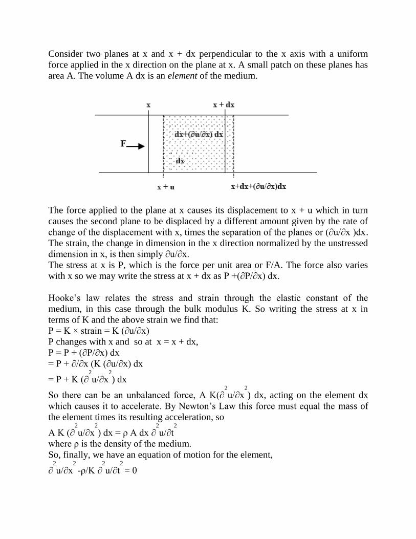
Consider two planes at x and x + dx perpendicular to the x axis with a uniform

force applied in the x direction on the plane at x. A small patch on these planes has

area A. The volume A dx is an element of the medium.

The force applied to the plane at x causes its displacement to x + u which in turn

causes the second plane to be displaced by a different amount given by the rate of

change of the displacement with x, times the separation of the planes or (∂u/∂x )dx.

The strain, the change in dimension in the x direction normalized by the unstressed

dimension in x, is then simply ∂u/∂x.

The stress at x is P, which is the force per unit area or F/A. The force also varies

with x so we may write the stress at x + dx as P +(∂P/∂x) dx.

Hooke’s law relates the stress and strain through the elastic constant of the

medium, in this case through the bulk modulus K. So writing the stress at x in

terms of K and the above strain we find that:

P = K × strain = K (∂u/∂x)

P changes with x and so at x = x + dx,

P = P + (∂P/∂x) dx

= P + ∂/∂x (K (∂u/∂x) dx

= P + K (∂2

u/∂x2

) dx

So there can be an unbalanced force, A K(∂2

u/∂x2

) dx, acting on the element dx

which causes it to accelerate. By Newton’s Law this force must equal the mass of

the element times its resulting acceleration, so

A K (∂2

u/∂x2

) dx = ρ A dx ∂2

u/∂t2

where ρ is the density of the medium.

So, finally, we have an equation of motion for the element,

∂2

u/∂x2

-ρ/K ∂2

u/∂t2

= 0

Since we normally deal with oscillatory or quasi-harmonic disturbances we can

explore the behavior of solutions to this equation by assuming that the solution in

time is sinusoidal and that the time dependence is given by eiωt

,

where ω is the angular frequency in radians/sec (equal to 2πf, where f is the

frequency in cycles per second or Hertz). With this solution in t the equation of

motion becomes:

∂2

u/∂x2

+ω2

ρ/K u = 0

or, with ω2

ρ/K = k2

∂2

u/∂x2

+k2

u = 0

The solution for the displacement u is,

u(x,t) = u0 e

iωt

e±ikx

= u0 e

i(ωt±kx)

This solution is basically the definition of a propagating wave. At a fixed position

in x, a particular element of the medium oscillates back and forth in the x direction

about a rest position (corresponding to the in-line oscillation of a particular mass in

the above mass-spring analog). At a fixed time the displacements are distributed

sinusoidally along x just as the spring distortions were distributed in the mass-

spring analog.

Another way to visualize the solution is to imagine the movement of a molecule or

particle in the liquid. The particle movement would be back and forth along the x-

axis, an oscillatory movement in the direction of propagation. At this microscopic

level the masses in the mass-spring analog are like particles in the liquid.

The derivation for compressive-extensional waves in a thin rod is identical except

that the bulk modulus is replaced by Young’s modulus, E.

The exponent ωt ± kz is called the phase and we can easily see what is required to

stay at a point in x and t where the phase is constant. When ωt ± kz = C, ∂z/∂t =

±ω/k which is the velocity of the phase point, the phase velocity Vph

. The plus sign

is for a wave traveling in the plus x direction, the minus sign for one traveling in

the opposite direction.

Substituting for k, the phase velocity is given by:

Vph

= (K/ρ)1/2

The phase velocity is equal to the square root of the ratio of the bulk modulus to the

density. Denser fluids thus have lower velocity than lighter fluids. Gases follow the

same formula. The table below lists some densities and compressibilities and the

derived velocities for some common liquids and air.

The distance at a given time between two successive points of equal phase on the

wave is the wavelength, λ, and the time between two successive points of equal

displacement at a given position on the x axis is the period, T, of the wave.

The velocity, frequency, period and wavelength are all related as can be seen in the

following figure.

3. Seismic waves in a solid The derivation of the equation of motion for an element in a solid is basically the

same as that outlined above but it is much more complicated to the fact that the

restoring elastic forces include shear as well as compression. The detailed analysis,

done very well for example in Telford et al., shows that there exists a

compressional wave with particle motion in the direction of wave propagation and

also a shear wave with particle motion in the plane perpendicular to the direction of

propagation. The velocities of these waves are given in terms of the bulk and shear

modulii, K ,μ and density, ρ, viz.:

It is clear from these expressions that the P-wave velocity is always larger than the

S-wave velocity and that the S-wave is not viable in a medium with no shear

strength.

Why the shear modulus is involved in the P-wave velocity is not intuitively

obvious. The above derivation for the wave motion in a fluid is based on the fact

that the bulk modulus K relates the volumetric strain to a hydrostatic pressure field.

Although not depicted in the cross section the volume element is deformed equally

in each coordinate direction – the moving pressure field does not change the shape

of the element. In a solid the pressure disturbance is not hydrostatic and the shape

of the element changes under deformation. It is the difference in deformation in

different directions that brings the shear modulus into play in the resulting

equations of motion.

The particle velocity in a shear wave can be in any direction in the plane

perpendicular to the propagation direction and it has become conventional to

describe a shear wave by a component whose particle movement is in the

horizontal direction, the SH

wave and a component whose particle motion is in a

vertical plane, the SV

wave. Any S-wave propagating in any direction can always be

represented by a superposition of SH

and SV

waves.

The elastic constants are all interrelated and a consequence that is very useful

in the study of soils and rocks is that Poisson’s ratio (ν) can be determined from the

P and S wave velocities via the following equation;

Poisson’s ratio is theoretically bounded between 0 and 0.5 and for most rocks lies

around 0.25, so typically VP/V

S is about 1.7.

The values of P wave velocities in representative crustal rocks are shown in the

following Figure:

4. Surface waves

On the surface between a solid or liquid and air the deformation of an element is

unconstrained in the direction normal to the surface. This changes the equation of

motion for elements or particles adjacent to the surface and gives rise to another

wave type commonly called the surface wave. Water waves are familiar and are

readily seen as having a much lower velocity than a sound wave propagating

through the bulk of the medium. Further a particle moves up and down vertically as

well as in the direction of the wave. In detail a particle traces an ellipse with a

prograde rotation as shown in the sketch below.

The surface wave on an isotropic half -space is known as a Rayleigh wave

and it is similar in form to the surface wave on a liquid half-space except that the

particle motion is retrograde. Rayleigh waves carry a large

amount of energy away from surface sources and are the noticeable, or ‘felt’,

ground motion when one is standing near a seismic source. In exploration

seismology Rayleigh wave are known as ground roll.

The velocity of a Rayleigh wave, VR, is tied to the S-wave velocity and

Poisson’s ratio (and hence to VP) through the solution to the following equation

(White, 1983)

The two plots below are taken from Mavko et al., 1998.

They show that for typical values of Poisson’s ratio the Rayleigh wave velocity

varies only from 0.91 to 0.93 VS.

The amplitude of the particle displacement for surface waves decreases

exponentially beneath the surface and the exponent is proportional to the frequency

as well as the elastic constants and density of the medium. Since it is observed that

velocity generally increases with depth, Rayleigh waves of high frequency

penetrate to shallow depth and have low velocity whereas Rayleigh waves of low

frequency penetrate to greater depth and have high velocity. The change in velocity

with frequency is known as dispersion. For a typical surface source of Rayleigh

waves the initiating disturbance has a broad frequency spectrum so the observed

surface motion at some distance from the source is spread out in time, with low

frequencies coming first and high frequencies coming later.

Measured Rayleigh wave dispersion can be used to invert for the vertical

velocity profile.

Finally, where the shear wave velocity increases with depth from the surface,

Love showed that a horizontally polarized surface wave could exist. This wave,

now called a Love wave, is also dispersive, and measurements of

it’s dispersion can also be inverted to find the distribution of shear wave

velocity with depth. Love waves require a distinct shear component in the source

stress field so they are not a strong component of the disturbance propagated from

the explosive or surface impact sources used in seismic exploration. They can be,

and are, generated by special horizontal shear sources. For many shallow

earthquakes they may be the dominant surface wave. This is a major factor used in

discriminating between underground nuclear explosions and shallow earthquakes.

5. Wavefronts, rays and geometrical attenuation

Until now we have concentrated on the physics of stress-strain fields and

their propagation in homogeneous solids and liquids. The fields arising from actual

natural or artificial sources and what happens to such waves when they encounter

inhomogeneities in density or elastic modulii is the real subject of interest. These

are the properties that we wish to extract from measurements of the waves that

have propagated into the earth.

To begin, an assumption is made that a point source is responsible for the

resulting seismic wave. In the case of an explosive source it is assumed that an

impulse of radially directed compressive force is created at a point. Similarly a

hammer hitting a small steel plate on the surface is considered a point source of

vertical compressive force. Such simple concepts immediately run into practical

limitations (what if the ground surrounding the explosive is itself inhomogeneous,

or the charge is close to the free surface? The stress field of the steel plate is not

hemispherical and there is, in practice a strong component of shear stress along the

edges of the plate.).

Considering the ideal compressive source at point O on a homogeneous half-

space, the resulting seismic P-wave propagates such that all the points of constant

phase lie on a hemisphere centered at O. The surface of all points of the same phase

is called a wave front although the inferred meaning is that the phase in question is

associated with some identifiable first arrival of the wave. A more rigorous

definition is that the wave front is the surface of all equal travel times from the

source. A cross section of such a hemispherical spreading wave is shown in the

following cartoon for two successive time steps, t1 and 2t

1.

The wave in this cartoon is really a wavelet, the impulsive short wave train

generated by the first compression of the source region, its subsequent recovery and

perhaps a few highly damped oscillations. (The source deformation is large, not

infinitesimal, and non-linear. Energy is dissipated in irreversible deformation

(damage) to the surroundings, and the pulse dies quickly as suggested by the

cartoon ‘source function’).

For convenience is describing wave propagation, the vector perpendicular to a

wave front is defined as a ray. The ray in the cartoon is directed along a radius

from the source, but this is not always the case. Rays are useful for describing what

happens to waves when they pass through an interface and we will use them later to

describe reflecting and refracting waves in layered media.

A numerical simulation of a seismic P-wave propagating away from a point source

is shown in the following movie. In the movie the amplitude of the wavelet is

contoured and color-coded. The high amplitude values are in red and the low

amplitude in blue in this plot. The zero of the wavelet is the color of the undistorted

background half-space. The time traces of geophones located in a well in the right

hand side of the section are shown in the graph on the right of the figure. This is the

fundamental form of the traces recorded in the vertical seismic profiling (VSP)

method.

6. Amplitude and energy

The energy imparted to the wave is proportional to the square of the amplitude of

the resulting propagated wavelet. Barring actual non-elastic losses in the medium,

the energy is conserved but is spread over the hemispherical shell that contains the

wavelet. The energy in a volume element of this shell at radius r is roughly the total

energy of the disturbance, E0, divided by the area of the hemisphere, 2/3πr

2

. The

energy in the wavelet thus falls off, or attenuates, as 1/r2

. The energy in the wavelet

is proportional to the square of the amplitude of the wavelet, so the amplitude of

the spherically spreading wave falls off as 1/r. The second wave front at

2t1

in the above cartoon is twice as far from the source as the first and so the

amplitude of the wavelet is reduced by half. This is called the geometric attenuation

and it is separate from any other attenuation due to loss mechanisms in the medium.

Surface waves spread in circular patterns from a point source (think water waves

spreading from the impact point of a stone) and in this case the energy decays as

1/r from the source and the amplitude consequently falls as 1/√r.

At very large distances from the source, the curvature of the wave front becomes

small and in some situations it is possible to neglect the curvature and assume that

the wave front is a plane. Such a wave is then known as a plane wave.

Seismic velocity, attenuation and rock properties

• Rock properties that affect seismic velocity

Porosity

Lithification

Pressure

Fluid saturation

• Velocity in unconsolidated near surface soils (the weathered layer)

• Attenuation

Seismic surveys yield maps of the distribution of seismic velocities, interfaces

between rock units and, ideally, of reflection coefficients at these interfaces. The

velocities of crustal rocks vary widely as the following figure shows.

Generally, the velocities depend on the elastic modulii and density via:

These elastic constants, and densities, in turn depend on the properties that the

geologist or engineer use to characterize the rock such as porosity, fluid saturation,

texture etc. A review of the relationships between the intrinsic rock properties and

the measured velocities or reflectivities is needed before seismic survey results can

be interpreted quantitatively in terms of lithology. Many of these relationships are

empirical – velocities are found to be related to certain rock units in a given locale

by actual laboratory measurements on core samples of the rock or soil.

It is observed from seismic surveys that velocities generally increase with depth.

Densities also increase with depth so it must be that the bulk and shear modulii

increase faster than the density. In seismic exploration there are many empirical

relationships between velocity and depth of burial and geologic age.

The relationship between intrinsic rock properties such as porosity, fracture

content, fluid content and density and velocity underlie the empirical

relationships mentioned above.

Rock properties that affect seismic velocity

1) Porosity. A very rough rule due to Wyllie is the so called time average

relationship:

where φ is the porosity.

This is not based on any convincing theory but is roughly right when the effective

pressure is high and the rock is fully saturated.

2) Lithification.

Also known as cementation. The degree to which grains in a sedimentary

rock are cemented together by post depositional, usually chemical, processes, has a

strong effect on the modulii. By filling pore space with minerals of higher density

than the fluid it replaces the bulk density is also increased. The combination of

porosity reduction and lithification causes the observed increase of velocity with

depth of burial and age.

3) Pressure.

Compressional wave velocity is strongly dependant on effective stress. [For

a rock buried in the earth the confining pressure is the pressure of the overlying

rock column, the pore water pressure may be the hydrostatic pressure if there is

connected porosity to the surface or it may be greater or less than hydrostatic. The

effective pressure is the difference between the confining and pore pressure.]

In general velocity rises with increasing confining pressure and then levels off to a

“terminal velocity” when the effective pressure is high. The effect is probably due

to crack closure. At low effective pressure cracks are open and easily closed with

an increase in stress (large strain for low increase in stress—small K and low

velocity). As the effective pressure increases the cracks are all closed, K goes up

and the velocity increases.

Finally even at depth, as the pore pressure increases above hydrostatic, the effective

pressure decreases as does the velocity. Over pressured zones can be detected in a

sedimentary sequence by their anomalously low velocities.

4) Fluid saturation.

From theoretical and empirical studies it is found that the compressional wave

velocity decreases with decreasing fluid saturation. As the fraction of gas in the

pores increases, K and hence velocity decreases. Less intuitive is the fact that Vs

also decreases with an increase in gas content. The reflection coefficient is strongly

affected if one of the contacting media is gas saturated because the impedance is

lowered by both the density and velocity decreases.

Velocity in unconsolidated near surface soils (the weathered layer)

The effects of high porosity, less than 100% water saturation, lack of cementation,

low effective pressure and the low bulk modulus (due to the ease with which native

minerals can be rearranged under stress) combine to yield very low compressional

and shear wave velocities in the weathered layer. Vp

can be as low as 200 m/sec in

the unsaturated zone (vadose zone) – less that the velocity of sound in air!

Attenuation

It is observed that seismic waves decrease in amplitude due to spherical spreading

and due to mechanical or other loss mechanisms in the rock units that the wave

passes through.

The attenuation for a sinusoidal propagating wave is defined formally as the

energy loss per cycle (wave length) Δ E/E where E is the energy content of the

wave.

Mathematically, the propagating wave , get an added damping term

, so the solution becomes

[We can apply this to the definition of attenuation Δ E/E by substituting A2

for the

energy at two points at distance λ (the wavelength) apart and we find

There are many theories for explaining attenuation in rocks. Friction,

included by including a velocity term in the governing differential equation for the

displacement does not explain laboratory measurement. Various other damping

mechanisms such as viscous flow (Biot Theory) have some success but much

important work remains to be done in this area (especially for unconsolidated

material where the attenuation is very high). Some of the theories predict

attenuation as well as dispersion (the variation of velocity with frequency).

Experimentally it is found that the attenuation coefficient depends on frequency

and that there is little dispersion. In fact to a good approximation attenuation can be

described by . With x in meters and f in Hertz, a typical shale has a

. So at one Hertz the amplitude falls to A0/e at 10 km. But at 1000 Hz it

falls to A0/e in 10 m. The attenuation may be as much as 10 times greater in

unconsolidated sediments.

Another important attenuation mechanism is the reduction in amplitude of a wave

by the scattering of its energy by diffraction by objects whose dimensions are on

the order of the wavelength. If a is an average linear dimension of velocity

inhomogeneities then the attenuation coefficient is given approximately by:

So attenuation increases rapidly with decreasing wavelength. Consider attenuation

is an unconsolidated medium with a velocity of 250 m/sec and a frequency of 1000

Hz. Then, λ = 0.25 m, and α = a3

×256. The wave would fall to 1/e of its initial

amplitude when a = 157 m.

It might be reasonable to expect inhomogeneities with a characteristic

dimension on the order of 15 cm in the overburden so it is likely that the very high

attenuation observed in near surface unconsolidated sediments is due to scattering.

Reflection and Refraction

1. The geometry of reflection and refraction A wave incident on a boundary separating two media is reflected back into the first

medium and some of the energy is transmitted, or refracted, into the second. The

geometry of refraction and reflection is governed by Snell’s Law which relates the

angles of incidence, reflection and refraction to the velocities of the medium.

The cartoon below illustrates the ray geometry for a P-wave incident on the

boundary between media of velocity V1

and V2. The angles of incidence, reflection

and refraction, θ1,θ

1’, and θ

2, respectively are the angles the ray makes with the

normal to the interface.

Snell’s law requires that the angle of reflection is equal to the angle of incidence. It

further implies that if V2 is less than V1 the ray is bent towards the normal to the

interface as in the cartoon, but if V2 is greater than V1 the ray is bent away from the

normal.

It is instructive to observe the progress of a spherically spreading wave as it

impinges on a horizontal boundary between media of different velocity. The wave

fronts are definitely not planar nevertheless rays at the interface satisfy Snell’s

Law. As in the planar model used to derive Snell’s Law, each point on the interface

where the spreading wave hits becomes the source of new waves which propagate

back into medium one and on into medium 2. In the following movie the spreading

wave is reflected at the interface and refracted into a medium of lower velocity.

angle of refraction is greater than the angle of the 1

Vis greater than 2

VIf

° . The = 902 θincidence. The latter result can lead to a special condition where

. The critical c

θcritical angle, angle of incidence for which this occurs is called the

angle is given by;

The geometry of this wave is correctly given by Snell’s law but the nature of a

wave that propagates along the interface is not so simple. The critically refracted

wave is a disturbance that propagates along the interface with the velocity of the

lower medium. As it goes its wave front acts as a moving

source of waves that propagate back into the upper medium with velocity V1

along

rays which are parallel to the reflected wave at the critical angle. This phenomenon

is illustrated in the following cartoon.

The following movie shows the propagation of an expanding wav front as it moves

through such a boundary.

The wave front in the lower, higher velocity, layer moves faster than the incident

wave front along the boundary. In the plane of the boundary this creates a stress

disturbance which travels along the boundary with velocity V2

and at each point

acts as a source for waves propagating back up to the surface. This wave is

commonly known as a Head wave and its wave front is clearly seen beyond the

point on the interface where the incident ray is at the critical angle.

In the description of reflection and refraction up till now we have not discussed the

physics of why a seismic wave is reflected only what the geometric relationship of

the wave fronts must be as the wave crosses an interface. The energy that is

reflected is determined by using the form for the solution for the particle

displacement (e.g. the form that we saw for a wave traveling in the x

direction) for a wave traveling towards an interface (the incident wave), one

traveling away from the interface in the opposite direction to the incident wave (the

reflected wave) and finally one transmitted into the second medium. At the

interface these general solutions must satisfy the boundary conditions: the

displacement across the interface must be continuous and both the normal and

tangential stress must be continuous.

For a P wave incident at an arbitrary angle these boundary conditions cannot be

met without incorporating an SV

wave as a reflected and transmitted wave. Thus it

appears that the incident P wave generates an SV

wave at the interface. Note that the

SV

waves leave the interface at angles dictated by Snell’s Law:

The solutions for the amplitudes of the various P and SV

waves for a P wave

incident at an arbitrary angle are given by the Zoeppritz Equations. In general they

yield complex results that cannot be summarized in this introductory treatment. The

analysis of the amplitude of the reflected waves as a function of incident angle,

which in practice means as a function of shot-point geophone off-set, yields

valuable information about the rock properties on either side of the interface. This

forms the basis of the important amplitude vs. offset (AVO) analysis of modern

reflection seismology.

The reflection coefficient for small off-sets is very close to that for normal

incidence, and since for normal incidence the stresses tangent to the interface are

zero, the dependence on the shear component disappears and no shear wave is

generated. The reflection coefficient from the Zoeppritz equations takes on a very

simple form:

Note that it is the energy that is conserved in reflection and transmission and the

energy is proportional to the square of the amplitudes of the waves. The energy

reflection coefficients are the squares of the above amplitude reflection

coefficients. This is important because it will be noted that the sum of the fraction

of the amplitude reflected and the fraction transmitted do not generally add up to

one whereas the energy coefficients do.

Time – Distance Plots • Reflection time-distance plots

• Moveout

• Dip moveout

• Reflection survey configuration

• Geophone arrays and spacial filtering

• Migration

• Refraction time-distance plots

• The ray-tracing algorithm

In surface seismic surveys the ‘point’ source is located on the surface and

detectors of the resulting seismic waves are located on the surface. The data of a

survey are the arrival times of the wave fronts at various distances from the source.

We have already seen a sample of this in the seismic time-traces that would be

observed at geophones placed in a well adjacent to a surface source. The data are

usually plotted with the arrival time on the vertical axis and the separation on the

horizontal axis. The following cartoon shows a hypothetical surface reflection

survey in which an array of 8 geophones is placed along a line on the surface at

equal intervals from the source, S (usually called the shot point). The geophones in

this example are located at 40, 80, 120, to 320 m, the layer is 200 m thick and the

velocity is 500m/s.

The plot of wavelet arrivals vs. time at any particular geophone location is a

recording of the ground motion at that geophone. This is the data recorded in a

seismic survey and it is usually called the seismogram. The above schematic result

is consequently known as a synthetic seismogram. The actual seismogram is

considerably more complex because it displays the ground roll, refractions if there

are any, and shear wave arrivals from part of the incident wave energy that is

converted to shear energy at the interface.

The travel time curves for models with layered dipping interfaces can be calculated

analytically and these formulas are well described in the standard texts referred to

in the introduction to this chapter. These solutions should always be used to check

any of the more general modeling codes.

The real world is rarely uniformly layered, certainly not with uniform layers of

constant velocity. It is known that in sedimentary rocks the velocity increases with

depth even in what appears to be a uniform depositional sequence. Further,

velocities can vary laterally in a given geological unit because of depositional

variation in grain size, clay content or degree of cementation. Finally the

subsurface has structure. The goal of shallow surveys is often to map the depth to

bedrock and this bedrock interface is unlikely to be a planar surface. Sedimentary

layers have faults, anticlines, folds, and unconformities which are in fact the very

features that trap petroleum and are the targets of the seismic exploration program

in the first place.

The major task of modern exploration seismology is to develop models of

the subsurface and methods of data processing which can be used to interpret the

complex wave front arrivals on a typical seismogram. The numerical modeling

programs that are used to create synthetic seismograms range from full 3

dimensional (3D) finite element or finite difference solutions to the governing wave

equation to approximate solutions that trace the progress of particular rays through

the medium. In this course we have adopted a general ray tracing program for

creating travel time curves. This code will be used for modeling reflections and

refractions from simple planar interfaces in the discussion that follows.

Reflection time- distance plots

Consider a source (shot point) at point A with geophones spread out along the x-

axis on either side of the shot point.

This is the equation of a hyperbola symmetric about the t axis. The travel time plot

for the direct wave arrivals and the reflected arrivals are shown in the following

plot. The first layer is 100 m thick and its velocity is 500 m/s. The intercept of the

reflected arrival on the t axis, ti, is the two-way zero

offset time and for this model is equal to 400 ms. At large offsets the hyperbola

asymptotes to the direct wave with slope 1/V1.

In most seismic reflection surveys the geophones are placed at offsets small

compared to the depth of the reflector. Under this condition an approximate

expression can be derived via:

Since is less than 1, the square root can be expanded with the binomial

expansion. Keeping only the first term in the expansion the following expression

for the travel time is obtained:

This is the basic travel time equation that is used as the starting point for the

interpretation of most reflection surveys.

Moveout

A useful parameter for characterizing and interpreting reflection arrivals is the

moveout, the difference in travel times to two offset distances. The following

expanded plot of one side of the hyperbola of the previous reflection plot shows the

moveout, Δt, for two small offsets.

Using the small offset travel time expression for x1 and x

2 yields the following

expression for the moveout:

The normal moveout (NMO), Δtn, is a special term used for the moveout when x

1 is

zero. The NMO for an offset x is then:

The NMO is readily measured with small offset reflection data. With the value of

the intercept time, ti , the velocity is determined via:

=

For a given offset the NMO decreases as the reflector depth increases and/or as the

velocity increases.

In a layered medium the velocity obtained from the NMO of a deep

reflector is an average of the intervening layer velocities. Dix (1955) found

that the root-mean-square velocity defined by:

is the travel time in layer i is the best

i nd tis the velocity in layer i a

i where V

average to use.

In interpretation the NMO’s for successive reflections are used to obtain the

average velocity to each reflector. Assuming these are the Vrms

velocities defined

above then Dix (1955) showed that the velocity in the layer bounded by the nth

and

n-1th

layer is given by:

Dip moveout

If the interface is dipping as in the figure below the up-dip and down-dip travel

times are changed by an amount dependant on the dip angle θ. The time-distance

plot is still a hyperbola but the axis of symmetry is shifted up-dip by 2h sinθ.

(Shown by the dashed line in the figure. Note also that the depth is still the

perpendicular distance from the interface to the shot point). The binomial

expansion for the travel time for small offsets becomes:

For geophones offset a distance x up-dip and down-dip, the dip moveout is defined

as:

For small dips when the dip moveout yields the dip via;

The velocity can be obtained with sufficient accuracy by averaging the velocities

obtained in the usual manner from the up-dip and down-dip NMO’s.

Reflection survey configuration

There have been many configurations of shot point and geophone arrays used over

the years. One important array is illustrated in the figure below. The geophone

array, also called the spread, is laid out almost continuously along the profile. Shots

are placed at the same locations as the geophones. At each shot point, Si, recordings

are made of the seismic record at each n geophones on either side of Si. After a

succession of shots e.g. Si+1

, Si+2,

Si+3,

the geophone traces corresponding to rays

that reflect at a common depth point (CDP) are collected and plotted.

This collection of records is also called a common mid point array. The advantage

of such an array is that many reflections from the same portion of the reflecting

interface can be averaged.

The resulting gather of traces will of course show the typical moveout of the

reflector but now all the rays reflect off the same point (the assumption is made that

the layer has a very small dip otherwise the rays will not have a common reflection

point). In practice there are variations in moveout caused by near surface variations

in velocity so the moveouts of each trace will vary but because the reflection point

is common and an average moveout can be calculated from which the velocity can

be obtained.

The background ground motions at separate geophones are assumed to be random,

as are the variations in near surface velocity. With these assumptions one method

of averaging is to assume a velocity and shift each trace back to its zero offset

value by its moveout. If the data were perfect all the reflection arrivals would line

up horizontally and the traces could all be added together to form an average zero

offset trace. By successively

changing the velocity until the maximum average reflection is obtained the

optimum velocity is determined. In this average trace the reflection event would be

well defined but the adjacent noise would average towards zero. Even with

reflections with variable moveouts, the average will lead to something greater than

the noise average so this process still leads to the selection of an optimum velocity.

This process of shifting and averaging the pairs of traces is called a CDP gather.

The final averaged time trace is plotted directly beneath mid point of the pairs

making up the gather. In practice, up to 64 common mid point shot-receiver pairs

may be averaged with this single CDP trace. (The number of pairs averaged in this

manner is referred to as the fold of the CDP gather.) The entire process is repeated

to produce another CDP trace, one interval, Δx , farther along the spread.

For most reflection surveys the traces shown are CDP gathers.

Geophone arrays and spacial filtering

A major problem in reflection surveying is the presence of a large amplitude

Rayleigh wave. Including the Rayleigh wave in a typical trace time plot for a deep

reflection usually shows that the Rayleigh wave often arrives just in the time

window of short offset reflections.

The Rayleigh wave can be minimized by considering the seismic arrivals at two

geophones spaced at half the wavelength of the Rayleigh wave.

I

f the output of two such geophones is summed the Rayleigh wave will produce no

output. The reflected wave on the other hand is coming up at near vertical

incidence and will be doubled in the summed output. More geophones at the

correct spacing will continue to augment the reflected arrival while effectively

canceling the Rayleigh wave.

In practice each receiver location in a reflection survey consists of a group of

geophones whose spacing is chosen to cancel the Rayleigh wave. A test survey is

conducted first to determine the Rayleigh velocity and frequency from which the

wave length is determined from λ = V/f.

Migration For any reflection array the interpreted refection point is plotted directly beneath

the mid point of the shot receiver separation. This is a plotting convention because

information about the possible dip or reflector

geometry is not generally available in the simple offset data. The apparent vertical

section is distorted by this means of plotting because the actual reflector point is

plotted beneath the mid point.

Consider the following sloping step on a reflecting interface. Assume the velocity

is known. The plots for the for the zero offset reflection (e.g. The CDP gather) are

plotted on the model. On the left and right of the sloping section the reflection

section mimics the actual section. However for reflections such as ABA, which

occur from point B on the slope the plotted point is at B1 –

displaced to the right of

the actual reflection point. Its ‘depth’ is just where the arc of radius AB intersects

the vertical beneath A. The net effect is that the plot of apparent reflection points

shifts the interface to the right and changes its slope.

This description also suggests the means to correct the section. Whenever a sloping

interface is found in the zero offset section the points on this interface are moved

back along an arc centered at the shot point. The line tangent to all the arcs is the

true position of the interface. The process

of shifting an apparent slope back to its true position in space is known as

migration.

Refraction time-distance plots

A typical ray path for an incident ray refracted at the critical angle is made up of

the lines ABDE shown in the figure below. The incident ray at the critical angle,

AB, yields a reflection BC and generates the head wave which propagates along the

interface. The wave front of the head wave generates waves which return to the

surface along rays which leave the interface at the critical angle, e.g path DE in the

figure. The refraction arrivals consequently begin at the same time as the reflected

wave on path ABC. Subsequent refraction arrivals are delayed by their travel time

along the interface at the velocity of the lower medium.

The equation for the travel time to an arbitrary point on the surface is

the sum of the travel times along AB, BD, and DE. The first and third times

are identical so:

Using the geometry imposed by Snell’s Law this becomes:

Since θc is determined via the velocities, then the equation can be

rewritten in terms of velocity as:

This is the equation of a straight line with slope and an intercept on the t axis,

This is the mathematical intercept; there are no refracted

arrivals at distances less than AC or at times less than the reflection travel time for

the ABC path.

The velocities can be determined directly from the travel time plot as the inverse of

the slopes of the direct and refracted arrivals so the depth can be determined from

the intercept time via:

The distance AC at which the first refraction arrives, called the

critical distance, xc , can be obtained from:

so

Finally it can be seen from the time-distance plot that there is a distance after which

the refracted arrivals come before the direct arrivals. This occurs at the crossover

distance, xcross

, when the refraction and direct waves have equal travel times, i.e

when

This is another useful equation for determining h. In practice with real data it is

usually found that projecting the refracted arrivals back to the t axis to find the

intercept time is more accurate than estimating where the crossover distance is.

The refraction arrivals from shot points at each end of a survey line over a dipping

interface are shown in the following figure:

The arrivals at geophones down dip from shot point A come at progressively later

times than their horizontal interface counterparts so that the slope of the arrival

curve is steeper. The apparent velocity obtained from the plot, Vapp down dip

, is less

than V2.

The apparent up dip velocity obtained with geophones up dip from shot

point B is greater than V2. The travel times from A to B and from B to A, the

reciprocal times, must be the same. Refraction surveys must be shot in both

directions. Arrival times taken in only one direction and interpreted as being taken

over a horizontal interface may yield erroneous results if the interface is dipping.

The equations for the travel times for a dipping interface, and for multiple layers

with dipping or horizontal interfaces, are derived analytically

in Telford et al.(1990) and they present a useful collection of expressions for

finding the depths and dips for up to three layer models.

A particularly useful result for small dips is that

are abbreviations for the down dip and up dip apparent velocities

u and V

d where V

respectively.

General expressions have been derived for the travel times for any number of layers

with accompanying equations for depths and true velocities but the quality of the

field time-distance data makes it difficult to identify intercept times or cross over

distances for more than a few refraction arrival segments. A better approach which

leads into general methods of interpreting seismic data is to use a numerical

technique to generate arrivals in model of an arbitrary medium and then by a

process known as inversion adjust the parameters of the model to match the

observed data.

In summary the principal advantage of the refraction method over the reflection

method is that it depends only on measuring the first arrival times on a seismic time

trace. There is no problem separating the refracted arrival from other arrivals as

there is in picking reflection events. Problems or disadvantages are:

i) there is no evidence in the travel time plot for an intermediate layer(s) of lower

velocity than the layers enclosing it. Interpretation in this case, which assumes a

progressive increase in layer velocity with depth, will be in error.

ii) there are situations where, even with increasing velocity in successive layers, a

refraction arrival segment may be masked by a deeper higher velocity earlier

arriving segment.

iii) the surface distribution of geophones must extend to distances of several times

the anticipated depth of the refractor in order to identify the crossover distance and

to determine the slope of the refractor arrival plot.

iv) at the large off-sets required by iii) the arrivals may be very weak and

impractically big shot energies may be required

164

SOLVED PROBLEMS IN ELECTRICAL & EM

1. Determine the potential difference between the two potential electrodes for

cases (a) and (b). Assume a current of 0.6 ampere.

(a)

VP1

i

2r1

i

2r2

i

2

1

r1

1

r2

i

2

1

12.17 m

1

21.63 m

VP1 0.686 v

VP2

i

2

1

12.65 m

1

20 m

VP2 0.555 v

VP1 VP2

0.131 v

(b)

VP1 0.418 v

VP2 0.418 v

VP1 VP2

0.836 v

165

2. Construct the current-flow lines beneath the interface in (a) and (b).

(a)

tan 1

tan 2 2

1

tan 2 tan 70 Þ 20 ohm m

200 ohm m

2 15 . 4 Þ

(b)

2 66.6Þ

166

3. Calculate the potential at ρ1, due to a current at C, of 0.6 ampere. The material in this

section view extends to infinity in all directions. The bold line represents an interface

between p1- and p2-material.

3.

VP1

i1

4r1

ik1

4r2

, k 2 1

2 1

0.6

VP1

0.6amp 200 ohmm

4 10 m

0.6amp 0.6 200 ohmm

4 16.67m

VP1 0.611 v

167

4. The following data were acquired using a constant-spread, Wenner traverse (a-

spacing = 3m). Interpret the data as completely as possible.

Horizontal

Position

(m)

Horizontal Horizontal

pa Position (m)

pa Position (m) Pa 5

20.05 19.00

22.55 33.00 858.94

6

20.06 20.00

25.32

34.00

872.33

7.00

20.07 21.00

28.45

35.00

880.40

8.00

20.08 22.00

27.97

36.00

885.58

9.00

20.10 23.00

27.11

37.00

889.07

10.00

20.12 24.00

242.39

38.00

891.51

11.00

20.15 25.00

460.00

39.00

893.26

12.00

20.19 26.00

572.39

40.00

894.57

13.00

20.24 27.00

580.25

41.00

895.55

14.00

20.32 28.00

541.30

42.00

896.31

15.00

20.44 29.00

519.88

43.00

896.90

16.00

20.61 30.00

660.54

44.00

897.38

17.00

20.91 31.00

785.22

45.00

897.76

18.00

21.45 32.00

834.74

This data suggests a vertical discontinuity at 25 m horizontal position. Resistivity

of the material to the left of the contact is 20 ohm·m and that of the material to the

right is 900 ohm·m.

168

5. The following data were gathered with a Wenner, expanding-spread traverse in an

area with thick alluvial deposits at the surface. What is the likely depth to the water

table? Electrode Spacing pa Electrode Spacing (m) pa

0.47 198 6..81 84

0.69 160 10..00 82

1..00 140 14.68 92

1.47 112 21.54 101

2.15 95 31.62 100

3.16 84 46.42 102

4.64 79

A consistent model shows that layer 1 is 1.3 m, 207 ohm·m; layer 2 is 15.7 m, 77

ohm·m; layer 3 is 107 ohm·m. A variety of input models produce similar results.

The water table, therefore, is judged to be at a depth of approximately 1.3 m.

169

HOMEWORK ASSIGNMENTS IN ELECTRICAL METHODS

1. CONSIDER A VERTICAL CONTACT BETWEEN TWO GEOLOGIC UNITS OF GREATLY

DIFFERENT RESISTIVITIES P1 AND P2 .

A. CALCULA TE THE DIRECTION THAT ELECTRICAL CURRENT WILL LEAVE THE BOUNDARY

INTO P2 IF IT APPROACHES THE BOUNDARY AT AN ANGLE OF 45° TO THE NORMAL.

B. CALCULATE THE ELECTRICAL POTENTIAL AT POINT A FROM A SINGLE SOURGE OF CURRENT (

+I ) A T POINT B. REMEMBER THAT THE BOUNDARY WILL CREATE A REFLECTED IMAGE OF

THE CURRENT SOURCE WITH MAGNITUDE KI. FOR P1 = 100 Ωm AND P2 = 0.1 Ωm

C. REPEAT (A) AND (B) FOR P1 = 100 Ωm AND P2 = 10000 Ωm

170

2. Determine the potential difference between the two potential electrodes for cases (a) and (b). Assume a

current of 0.5 ampere for (a) and 0.8 ampere for (b).

3. Construct the current-flow lines beneath the interface in (a) and (b).

171

4 - Interpret the following data, which were obtained with a Schlumberger traverse.

Electrode Spacing (m)

( Ω . m) Electrode

Spacing (m)

( Ω . m) Electrode

Spacing (m)

( Ω . m)

I.00

108

14.68

307

215.44

293 1.47

121

21.54

245

316.23

381 2.15

I4X

31.62

168

464.16

479 3.16

191

46.42

122

681.29

580 4.64

244

68.13

115

1000.0 675

6.81

295

100

162

10.00

323

146.78

220

5- The following data were gathered with a Wenner, expanding-spread traverse in an area of thick

deltaic sands. Bedrock depths are greater than 30 m. What is your best estimate of the depth to the

water table in this area?

Electrode Spacing (m) ( Ω . m) Electrode Spacing (m) ( Ω . m)

0.47

2590

6.81

8753

0.69

3288

10.00

7630

1.00

4421

14.68

4805

1.47

5198

21.54

2160

2.15

6055

31.62

995

3.16

6686

46.42

584

4.64

7782

6. The following data were gathered with a Wenner. expanding-spread traverse in an area of dune sands

underlain by lake clays which in turn are underlain by Triassic sedimentary rocks. Estimate a

value for clay thickness.

Electrode Spacing (m) ( Ω . m) Electrode Spacing (m) ( Ω . m)

0.69

1298.90

10.00

360.67

1.00

1398.06

14.68

240. 1 1

1.47

1306.98

21.54

191.51

2.15

1153.02

31.62

153.81

3.16

925.27

46.42

116.38

4.64

762.40

68.13

98.03

6.81

554.13

100.00

86.08

172

7. Interpret the following data, which were obtained with a Wenner traverse.

Electrode Spacing (m)

pa (Ω • m)

Electrode Spacing (m)

pa (Ω • m)

Electrode Spacing (m)

pa (Ω • m)

1 .00 984 14.68 72 215.44 327

1.47

955

21.54

53

316.23

432

2.15

883

3 1 .62

63

464.16

554

3.16

742

46.42

87

68 1 .29

686

4.64

533

68.13

124

1000.00

818

6.81

311

100.00

174

10.00

150

146.78

241

8. Assume a homogeneous medium of resistivity 120 ohm-m. Using the wenner electrode system with a 60-m spacing, assume a current of 0.628 ampere. What is the measured potential differ-ence? What will be the potential difference if we place the sink (negative-current electrode) at inf i n i t y ?

9. Suppose that the potential difference is measured with an electrode system for which one of the current electrodes and one of the potential electrodes are at infinity. Using the Figure below and a current of 0.5 ampere, compute the potential difference between the electrodes at PA and infinity for d1 = 50 m, d2 = 100 m, R1 = 30 ohm-m, R2 = 350 ohm-m.

173

10. Plot resistivity data as a function of electrode spacing, and determine the particular electrode spacing corresponding to the inflection point for the data given in Exercise 9. Compare the electrode spacing at the inflection point with the depth of the boundary from Exercise 9.

11. If the Schlumberger electrode system with AB/2 : MN/2 = 5. is used to conduct the resistivity

survey explained in Exercise 9, what will the potential readings be? Use resistivity values found in Exercise 9 to compute potential differences for each of the electrode spacings AB/2 = 1, 2, 4, 6, 8, 10, 15, 20, 25, 30, 40, 50 m whi le a constant cu r ren t of 0.250 ampere is applied.

12. Suppose that an electrical resistivity survey was done using an expanding Wenner electrode-

configuration. The current of 0.25 ampere was kept the same for all the readings. Potential d i f -ferences measured with different electrode spacings are given in the following table. Interpretations of these measurements indicate that a layer of resistivity R1 lies above another layer of resistivity R.2. Determine the depth of the boundary between these two layers. Estimate the resistivities of the layers.

ELECTRODE SPACING (m) POTENTIAL DIFFERENCE (v)

1 0.8

2 0.42

4 0.28

6 0.155

8 0.125

10 0.120

15 0.105

20 0.10

25 0.098

30 0.086

40 0.076

50 0.064

13. For purposes of an IP survey, resistivity values are determined from both direct and alternat ing current using the same electrode arrangement. If the resistivities for direct and alternating cur-rent are Rdc = 50 ohm-m and Rac = 40 ohm-m, respectively, what wi l l the frequency effect and the metal factor values be.

174

14. Assume- that a telluric current survey is to be carried out to outline large-scale features of a sedimentary basin 5 km deep. A resistivity of 50 ohm-m is supposed to represent the sedimentary section. What is the maximum frequency of the telluric current that will penetrate below the basin?

15. Suppose That a magnetotelluric survey indicates an apparent resistivity of 5 ohm-

m at a frequency of 1 Hz, What is the thickness of the layer?

16. Using the method of electrical images, drive therelationship between apparent resistivity,

electrode spacing, layer thicknesses and resistivities for a VES performed with a

Schlumberger spread over a single horizontal interface between media with resistivities ρ1

and p2.

17. Calculate the variation in apparent resistivity along a HEP profile at right angles to a

vertically faulted contact between sandstone and limestone, with apparent resistivities

of 50 ohm m and 600 ohm m. respectively, for a Wenner configuration. What

would be the effect on the profiles if the contact dipped at a shallower angle.

18. Why are the electrical methods of exploration particularly suited to hydrogeological

investigations? Describe other geophysical methods which could be used in this context,

stating the reasons why they are applicable.

19. Let A and B represent two different geologic sections, and let H1 and H2 represent the thicknesses of the

first and second layers in a three-layer sequence. It is well known that one type of equivalence

occurs for a three-layer case when p1 < p2 > p3 . p 1 A = p1B , p3A= p3B , H1A = H 1B , and P2A. H2A =

P2B. H2B . Demonstrate that this is true. Does equivalence exist if p1 > p2 < p3 ?. Explain.

175

20. At locations A, B, C , D along the gravity profile shown below, VES were performed with

a Wenner array with the spread laid perpendicular to the profile.

It was found that the sounding curves, were similar for locations A ,and B and for C

and D. A borehole close to A penetrated 3m of drift, 42 m of limestone and

bottomed in sandstone. Downhole geophysical surveys provided the following values

of density (D) and resistivity (ρR) for the lithologies encountered.

Unit

R (Ω m)

D ( Mg m-3)

Drift

40

2.00

Limestone

2000

2.75

Sandstone

200

2.40

A seismic refraction line near to D revealed 15m of drift, although the nature of the

underlying basement could not be assessed from the seismic velocity.

(a) Interpret the geophysical data so as to provide a geological section along the

profile.

(b) What further techniques might be used to confirm your interpretation?

(c) If a HEP were to be performed along the profile, select, giving reasons, a suitable

electrode spacing to map the basement. Sketch the expected form of the HEP for both

longitudinal and transverse traverses.

176

21. The following table represents the results of a frequency domain IP survey of a

Precambrian shield area. A dipole-dipole array was used with the separation ( x) of

both the current electrodes and the potential electrodes kept constant at 60m. n refers to

the number of separations between the current and potential electrode pairs and c to the

distance of the center of the array from the origin of the profile, where the results are

plotted (Figure below). Measurements were taken using direct current and an

alternating current of 10Hz. These provided the apparent resistivities pdc and pac

respectively,

(a) For each measurement point, calculate the percentage frequency effect (PFE) and

metal factor parameter (MF).

The dipole-dipole electrode configuration.

(b) For both the PFF, and MF plot four profiles for n = 1,2 , 3 and 4.

(c) The area is covered by highly-conductive glacial deposits 30-60m thick, It is possible that

massive sulphide mineralization is present within the bedrock. Bearing this information in

mind, comment upon and interpret the profiles.

177

22. For each of the following subsurface models sketch an appropriate apparent resistivity curve on the designated graph. The general shape of the curve is what is important. Base your curves on what you know about current penetration, current density, and measured resistivities.

(a) Layer Thickness (m) Resistivity ( Ω .m)

1 1 100

2 5 10

3 5 100

4

Infinite

1

(b) Layer Thickness (m) Resistivity ( Ω .m)

1 10 100

2 10 10

3 Infinite 100

178

23. The figure below shows a half-Schlumberger resistivity array in which the second

current electrode is situated at a great distance from the other electrodes. Derive an

expression for the apparent resistivity of this array in terms of the electrode spacings and

the measured resistance.

The half-Schlumberger electrode configuration. 24. Calculate the potential at P1 due to a current at C1 of 0.6 ampere. The material in this section view

extends to infinity in all directions. The bold line represents an interface between p1 and p2 –material.

179

PROBLEM SETS IN GEOPHYSICAL EXPL.

1. Given the reversed refraction observations (travel time vs. distance curves) shown below,

calculate the velocities and depths to the interfaces. Calculate the dip angles of the interfaces.

2. Given the following schematic travel-time curves, describe a subsurface structure and/or

velocity changes that may explain them.

180

3. A rock sample is taken to the lab and is subjected to a uniaxial stress (that is, it is stressed

in only one direction with the remaining directions free). As a result of the stress, the length

of the sample increases by 3% and the width decreases by 1%. What is the ratio of the P wave

velocity to the S wave velocity in this sample?

4. Two seismic reflection profiles are shot, the first along a north-south line and the second

along a line oriented 45o east of north. The first profile reveals an interface dipping to the

north at 20o, while the second reveals an interface dipping to the northeast at 35o. What is the

true strike and dip of the interface?.

181

5. A material has a shear modulus of 8.8×109 Pa, a bulk modulus of 2.35×1010 Pa, a density of

2200 kg/m3 and a quality factor Q = 100.

a) What are the P-wave velocity and S-wave velocity of the medium, in units of km/s ?

b) If a P-wave of frequency 10 Hz has a displacement amplitude of 1 µm at a distance of 10 m

from the source, what would be the wave amplitude at 100 m?

6. Near-surface fresh water in a Lake Superior has been observed to have a P-wave velocity of

1435 meters/sec. Estimate its bulk modulus, assuming it is pure water.

2. A laboratory has determined that the Gabbro has the following properties:

Bulk modulus= 0.952130 X 1012 dyne/cm2

Shear modulus=0.403425 X 1012 dyne/cm2

Density=2.931 gm/cc

Determine the (a) shear wave velocity, the (b) compressional wave velocity, and (c) Poisson's

ratio for this rock.

7. While attempting to put in a water-well near Longville, Minnesota, a driller encountered fresh granite at

"about 50 feet". Because the glacial till, which largely consists of unconsolidated clay and silt, is usually

thicker in this region, the driller first suspected that he had hit a boulder. Upon drilling a "few more feet",

however, the granite persisted, leading the driller to fear that he had indeed hit bedrock, and that further

drilling might result in an expensive and potentially unproductive water well.

A seismic refraction survey that used a sledge hammer for an energy source was conducted at the site to

investigate the depth to bedrock. The observed first breaks were as follows:

Dist. from t first break

source (ft.) (milliseconds)

---------------------------------- 5 5.19

10 9.74

30 21.8

60 34.9

90 40.7

120 46.7

150 51.1

180 54.3

210 59.3

240 65.5

270 72.2

300 75.2

330 79.8

A reversed profile (not given) was essentially identical, and, therefore, horizontal layering can be

assumed. Plot the travel time graph (x-horizontal, t-vertical) and assuming a two-layer model, estimate v1,

v2 and h1. Assuming a velocity of 18,000 feet/second for fresh granite,

do you see any evidence of granite bedrock in the profile? If so, what is the depth? If not, what is the

minimum depth that granite could occur?

Do you think that the driller hit bedrock or a very large boulder?

182

8. In Todd County, Minnesota a seismic refraction survey was conducted along an abandoned railroad

grade about 2.5 miles southeast of the town of Osakis. The railroad grade is known to be resting on

Pleistocene glacial deposits. A 12 channel system was used with an sledge hammer for an energy source,

and the following first break times were picked from the traces.

Distance First break time

(meters) (milliseconds)

5 14

15 23

25 30

35 36.75

45 42

55 50

65 54.5

75 61

85 65.5

95 66.5

105 70

115 73.25

A reversed profile yielded essentially identical results, so we can assume horizontal layering. It is assumed

that the first and second layers will represent the grade fill and the glacial deposits, respectively.

Plot the travel time relationships and estimate the velocities of the first two layers (in meter/second). What

is the thickness of the grade fill?

Based on your velocity estimate for the second layer, do you think the glacial deposits are saturated or

unsaturated (below or above the water table)?

Do you have any evidence of bedrock (ie a third layer) below the glacial deposits? If so, what is its

velocity (in meters/second) and depth?

9. FOR PURPOSE OF IP SURVEY, RESISTIVITY VALUES ARE DETERMINED FROM BOTH

DIRECT AND ALTERNATING CURRENT USING THE SAME ELECTRODE ARRANGEMENT. IF

THE RESISTIVITY FOR DIRECT AND ALTERNATING CURRENT ARE Rdc = 50 OHM.M AND Rac

= 40 OHM.M, RESPECTIVELY. WHAT WILL THE FREQUENCY EFFECT AND THE METAL

FACTOR VALUES BE.

10. DESCRIBE THE APPLICABILITIES OF SEIMIC AND ELECTRICAL ( WENNER,

SCHLUMBERGER, DIPOLE-DIPOLE) , AND GROUND PENETRATING RADAR (GPR )

METHODS FOR INVESTIGATING THE FOLLOWING TARGETS :

A. SOLUTION CAVITIES AND FRACTURES IN LIMESTONE FORMATION.

B. SPHALERITE AND GALENA (LEAD AND ZINC ORES ) MASSIVE SULFIDE

DEPOSITS IN A DOLOMITE / MARBLE FORMATION.

183

C. MAPPING OF SALWATER / FRESHWATER INTERFACE ; SATURATED AND

UNSATURATED ZONES IN COASTAL AREAS.

D. ARCHAEOLOGICAL APPLICATIONS

11. CALCULATE ELEVATION AND WEATHERING CORRECTIONS FOR THE THREE

GEOPHONE LOCATIONS IN THE ACCOMPANYING SKETCH.

12. SUPPOSE THAT A REVERSED REFRACTION SURVEY ( USING SHOTS A AND B )

INDICATED VELOCITIES V1 = 1500 M/SEC. AND V2 = 2500 M/SEC. FROM SHOT A AND

VELOCITIES V1 = 1500 M/SEC AND V2 = 3250 M/SEC. FROM SHOT B.

FIND THE DIP OF REFRACTOR. WHAT WOULD BE THE CHANGES IN VELOCITIES IF THE

FEFRACTOR HAD A SLOPE 10 DEGREES LARGER THAN THE ONE YOU COMPUTED.

13. SUPPOSE THAT THE POTENTIAL DIFFERENCE IS MEASURED WITH AN ELECTRODE

SYSTEM FOR WHICH ONE OF THE CURRENT ELECTRODES AND ONE FOR THE POTENTIAL

ELECTRODES ARE AT INFINITY. USING THE FIGURE BELOW, AND A CURRENT OF 0.5

AMPERE.

COMPUTE THE POTENTIAL DIFFERENCE BETWEEN THE ELECTRODES AT PA AND

INFINITY FOR d1 = 50 m, d2 = 100 m, R1 = 30 Ohm-m, R2 = 350 Ohm-m.

.14. A SET OF SEISMIC REFRACTIN FIELD DATA WAS COLLECTED FOR BOTH FORWARD

AND REVERSE SHOTS AS GIVEN BELOW :

DISTANCE ( FT) ELEVATION ( FT) ARRIVAL TIMES ( MSEC)

SHOT A SHOT B

0 (SHOT A ) 105 0 ---------

100 103 48 274

200 101 93 252

300 95 136 237

400 90 139 221

500 85 151 211

600 110 176 221

700 110 202 212

800 105 221 204

900 100 238 179

1000 105 237 136

1200 110 271 47

1300 (SHOT B) 95 ----- 0

184

A. PLOT T-X CURVE ( WITHOUT ANY CORRECTION ). ASSUMING A SLOPING LAYER,

OBTAIN AND PLOT THE SUBSURFACE STRUCTURE.

B. APPLY AN ELEVATION CORRECTION TO EACH STATION FOR THE ENTIRE

RECORDS. RE-INTERPRET THE T-X CURVE AND PLOT THE SUBSURFACE

STRUCTURE.

C. APPLY BARTHELEMES’ DELAY TIME METHOD FOR EACH SHOT POINT A

AND B. DRAW THE FINAL CROSS-SECTION OF THE SUBSURFACE ALONG

WITH THE SURFACE TOPOGRAPHY.

185

15. DETERMINE THE SUITABLE OIL ACCUMULATION FROM THE CROSS-SECTION

SHOWN.

Exercise No.( )

Complete the given geologic cross-section and determine the

suitable location of oil accumulation.

Q = Quaternary, L = hard Eocene limestone,

E = Eocene evaporite , S = Paleocene sandstone,

Sh = Upper Cretaceous shale, SL = sand lens,

R = coral reefs, B = Basment

QQQ

L

LL

L

Q

L

LL L

L

E

E EE

E

E

S

S

S

S

S

S

SS

S

Sh

Sh

Sh

Sh

Sh

Sh

Sh

Sh

Sh

Sh

Sh Sh

Sh

Sh

Sh

Sh

Sh

R

R

R

R

R

R

R

R

R

RR

B

BB B

B B B

B

SLSL

SL

SL

SLSL SL

Sh

Sh

Sh

186

16. The figure below shows waves travelling on a string whose right and left sides have a

different velocity and density.

a. Use the positions of the waves at successive times to find the velocity on

either side.

b. Measure the amplitude of the wave incident on the junction (dashed line)

at time 1, and the amplitudes of the reflected and transmitted waves at time

2. Find the reflection and transmission coefficients from the ratio of these

amplitudes.

c. Derive a relationship, using the expression for the transmission coefficient,

for the ratio between the densities of the two media. Which medium is the

more dense?

d. If the density of the right hand medium is 2 = 4 g / cm3, determine the

density of the left hand medium.

e. Do these waves more nearly represent P-waves or S-waves? Why?

187

17. Identify the four wave types shown (P or S). Assuming the P velocity in the solid is 13.5

km/s, find the P and S velocities in both media. (Hint: Use a protractor to measure the angles).

188

18. For a layer of thickness h, composed of material with velocity V0 above a half-space which

consists of material with a velocity V1, as shown below,

a. Express the travel time of the direct wave to the receiver as a

function of the source-receiver distance x.

b. Show that the travel time of the reflected wave can be represented as,

To test this, determine the travel time for the

reflection at zero distance (zero offset).

c. Express the critical angle ic as a function of the velocities V0 and V1 .

d. Show that the travel time for a critically refracted (or head) wave at a

distance x is;

e. Derive an expression for the minimum distance at which the refracted

wave may be observed in terms of the layer thickness h and the velocities

V0 and V1 .

f. Show that the crossover distance at which the direct and refracted wave

arrivals arrive at the same time is given by; .

g. Plot , and as a function of distance for h = 33 km, V0 =

6 km/s, V1= 8 km/s.

189

مصطلحات الإستكشاف الكهربائي والكهرومغناطيسي

المصطلح الترجمة العربية

Self Potential جهد ذاتي

Galvanometer مقياس الجهد الكهربائي

Apparent Resistivity مقاومية ظاهرية

Equipotential line خط متساوي الجهد

Principle of Equivalence مبدأ التعادل

Principle of Suppression مبدأ الغطس

Conductivity التوصيلية

Vertical Electrical Sounding الجس الكهربائي العمودي

Horizontal Electrical Profiling المقطع الكهربائي الأفقي

Dipole ثنائي القطب

Schlumberger Arrangement ترتيب شلمبرجير

Induced Polarization الإستقطابية المستحثة

Passive Methods الطرق الخامدة

Electrical Conduction التوصيل الكهربائي

Archie's Law قانون أرشي

Electrical Reflection Coefficient معامل الإنعكاسية الكهربائية

Ground Penetrating Radar (GPR) رادار الإختراق الأرضي

Airborne Electromagnetic المسح الكهرومغناطيسي الجوي

Very Low Frequency (VLF) التردد المنخفض جدا

190

مصطلحات الإستكشاف الجاذبي والمغناطيسي

Absolute gravity جاذبية مطلقة

Magnetic Field Strength قوة المجال المغناطيسي

Magnetic Induction الحث المغناطيسي

Centrifugal Force قوه طرد مركزية

Intensity of Magnetization شدة التمغنط

Magnetic Declination انحراف مغناطيسي

Diamagnetic ضعيف النفاذية المغناطيسية

Diurnal Correction تصحيح يومي

Elevation Correction تصحيح الارتفاع

Equator خط الاستواء

Magnetic Permeability النفاذية المغناطيسية

Ferro magnetic مغناطيس حديدي

Gravitational Acceleration التسارع الجاذبي

بيةشاذة الجاذ Gravity Anomaly

Magnetic Inclination الميل المغناطيسي

Isostatic Correction تصحيح ايزوستاتي

Lunar Variations تغيرات قمرية

Magnetic Moment العزم المغناطيسي

Magnetic Storms عواصف مغناطيسية

Magnetometer جهاز قياس المغناطيسية

ية المغناطيسية(قابلية مغناطيسية )التأثر Magnetic Susceptibility

Observed Gravity جاذبية مقاسة

Paleomagnetism مغناطيسية قديمة

Residual Magnetism مغناطيسية متخلفة

Remanent Magnetism مغناطيسية متبقية

Secular Variations تغيرات متناهية البطء

Geoid الجيوئد ) سطح متساوي الجهد (

هاز قياس الجاذبيةج Gravimeter

Bouguer Anomaly شاذة بوجير

Latitude Correction تصحيح خط العرض

191

مصطلحات الإستكشاف السيزمي

المصطلح الترجمة العربية Elasticity المرونة

Stress System نظام الإجهاد

Poisson’s ratio معامل بوايسون

Tangential Stress الإجهاد المماسي

Transverse Stress الإجهاد المستعرض

Transverse Strain التشوه )الانفعال( المستعرض

Normal Stress الإجهاد العمودي

Rigidity Modulus معامل الصلابة

Shear Modulus معامل القص

Hooke’s Law قانون هوك

Elastic Limit حد المرونة

Plastic Point نقطة اللدونة

واد اللامرنةالم Anelastic Materials

Shear resistance مقاومة القص

Young’s modulus معامل يونج

Compressibility الانضغاطية

Dilatation تمدد حجمي

Wave Propagation الانتشار الموجي

Body Waves الموجات الباطنية

Surface Waves الموجات السطحية

Longitudinal Waves الموجات الطولية

Primary Waves الموجات الأولية

Compressional Waves الموجات التضاغطية

Shear Waves موجات القص

Transverse Waves موجات مستعرضة

Secondary Waves موجات ثانوية

Birch’s Law قانون بيرش

Seismic Velocities سرع سيزميه

Rayleigh Waves (LR) موجات رايلي

Love Waves (LQ) موجات لوف

Dispersion تشتت

Amplitude سعة الموجة

Wavelength طول الموجة

Frequency تردد

192

Seismic Refraction الانكسار السيزمي

Seismic Reflection الانعكاس السيزمي

Critical Distance المسافة الحرجة

Thickness سماكة

Depth عمق

Seismic Source مصدر سيزمي

Transmitter مرسل

Receiver مستقبل

Geophones سماعات أرضية

Fermat’s Principle مبدأ فيرمات

Huygen’s Principle مبدأ هايجن

Reflection Coefficient (Rc) معامل الانعكاس

Transmission Coefficient (Tc) معامل الاختراق

Acoustic Impedance العائق الصوتي

Wavefront مقدمة الموجة

Raypath مسار الموجة

Snell’s Law قانون سنيل

Critical Refraction الانكسار الحرج

Low- Velocity – Layer طبقة منخفضة السرعة

Hidden Layer طبقة مختبئة

Blind Layer طبق عمياء

Thin Layer طبقة رقيقة

Diffraction الحيود

Delay Time زمن التأخير

Dipping Layers طبقات مائلة

Green Equation معادلة جرين

Dynamic Correction التصحيح الديناميكي

Multiple Reflection انعكاس متعدد

Time- Average Equation معادلة معدل الزمن

Faust Equation معادلة فوست Apparent Velocity سرعة ظاهرية

Average Velocity (VA) معدل سرعة

Interval Velocity (VI) سرعة بينية

Root Mean Square Velocity سرعة تربيع متوسط الجذر

Dix Equation معادلة ديكس

Data Processing معالجة المعلومات

Cross Over Distance مسافة العبور

Seismic Attenuation تعتيم سيزمي