an efficient tabu search approach for the two-machine preemptive open shop scheduling problem

Available online at www.sciencedirect.com

Computers & Operations Research 30 (2003) 2081–2095www.elsevier.com/locate/dsw

An e#cient tabu search approach for the two-machinepreemptive open shop scheduling problem

Ching-Fang Liaw∗

Department of Industrial Engineering and Management, Chaoyang University of Technology,168 Gifeng East Road Wufeng, Taichung, Taiwan

Received 1 March 2002; received in revised form 1 September 2002

Abstract

This article considers the problem of scheduling two-machine preemptive open shops to minimize totaltardiness. The problem is known to be NP-hard. An optimal timing algorithm is presented to determine thecompletion time of each job in a given job completion sequence. Then a tabu search (TS) approach isadopted together with the optimal timing algorithm to generate job completion sequences and 4nal schedules.An e#cient heuristic is developed to obtain an initial solution for the TS approach. Diversi4cation andintensi4cation strategies are suggested. Finally, computational experiments are conducted to demonstrate theperformance of the proposed approach. The results show that the proposed TS approach 4nds extremelyhigh-quality solutions within a reasonable amount of time.

Scope and purpose

Shop scheduling problems, such as 9ow, job and open shop problems, are widely used in the modelingof industrial production processes and are receiving an increasing amount of attention from researchers. Inan open shop scheduling problem, the order of processing the operations of a job on di;erent machines isimmaterial. Examples of open shop scheduling include teacher-class assignment, examination scheduling, andtesting/repair operation scheduling. The purpose of this paper is to examine the two-machine total tardinessopen shop scheduling problem with the assumption that the processing of an operation can be arbitrarilypreempted. An approximate solution method based on tabu search is proposed. Computational results showthat the proposed solution method performs well in terms of both solution quality and computation time.? 2003 Elsevier Ltd. All rights reserved.

Keywords: Scheduling; Open shop; Tabu search; Tardiness

∗ Tel.: +886-4-2332-3000; fax: +886-4-2374-2327.E-mail address: [email protected] (C.-F. Liaw).

0305-0548/03/$ - see front matter ? 2003 Elsevier Ltd. All rights reserved.PII: S0305-0548(02)00124-7

mailto:[email protected]

2082 C.-F. Liaw /Computers & Operations Research 30 (2003) 2081–2095

1. Introduction

The classical open shop scheduling model can be de4ned as follows. We are given n independentjobs and m parallel machines. Each job i; i=1; 2; : : : ; n, consists of m operations, Oij; j=1; 2; : : : ; m,where operation Oij of job i has to be processed on machine j for pij time units. At any time,at most one operation can be processed on each machine, and at most one operation of eachjob can be in process. The operations of a job can be processed in any order. The open shopscheduling model has received considerable research attention (see Refs. [1,2]) because it occursin many real-world scheduling environments. In many situations, particularly testing and mainte-nance, the order in which the operations are processed is immaterial. The teacher-class timetablingproblem is another example where the open shop model is a natural basic formulation. An openshop is similar to a job shop except that the operations of a job can be processed in any order.Relaxing the ordering constraints from a job shop yields a looser problem structure. This, how-ever, implies that the number of feasible schedules increases tremendously. Thus, the problem of4nding optimal open shop schedules by (implicit) enumeration is even more di#cult than it is forjob shops.

In this paper, we consider a special case of the open shop scheduling problem. We shall beconcerned with the case of m = 2 in which preemption is allowed. That is, there are only twomachines and the processing of any operation can arbitrarily often be interrupted and resumed at alater time. Each job i; i=1; 2; : : : ; n, is available at time zero and has a due date di. The objective isto 4nd a feasible schedule such that the total tardiness

∑ni=1 Ti =

∑ni=1 max(Ci−di; 0) is minimized,

where Ci is the completion time and Ti is the tardiness of job i. Following the three-4eld notationof Graham et al. [3], we denote this problem as Om|prmp|

∑Ti. The problem is NP-hard since its

special case with m = 1 is already a NP-hard problem [4].Most variations of open shop scheduling problems are known to be NP-hard. Polynomial time

algorithms only exist for a few special cases. A large number of studies have been done on thenon-preemptive scheduling of open shops [5–9]. When preemption is allowed, Gonzalez and Sahni[10] proposed a polynomial time algorithm for the problem Om|prmp|Cmax. Improved versions ofthat algorithm were given by Gonzalez [11]. Cho and Sahni [12] presented a linear programmingformulation for the problem Om|prmp; ri; Idi|Cmax where each job i has a release time ri and duetime Idi. They also gave polynomial algorithms for special cases of this problem. Lawler et al. [13]developed a linear time algorithm for the problem O2|prmp|Lmax. They also proved that the problemO2|prmp|

∑Ui is NP-hard. Liu and Bul4n [14] showed that both the problems O3|prmp|

∑Ci and

O2|prmp; Idi|∑

Ci are NP-hard. Liu and Bul4n [15] also studied the preemptive ordered open shopand proposed polynomial time algorithms for special cases of this problem.

Recently, Liu [16] developed an e#cient branch-and-bound algorithm for the problem Om|prmp|∑Ci. The algorithm was further generalized by Liaw [17] to solve the problem Om|prmp|

∑Ti.

However, the algorithm in [17] can only be used for small scale problems. In this paper we proposea tabu search (TS) algorithm for the problem O2|prmp|

∑Ti. For m = 2, an optimal schedule can

be constructed in linear time if the order of job completion times is known in advance. This resultmotivates us to use the TS approach as an alternative approach that has shown superiority in 4ndingoptimal or near optimal solutions for many problem settings.

The rest of the paper is organized as follows. In Section 2 we present a linear programmingformulation for the problem under consideration if the sequence in which jobs are completed

C.-F. Liaw /Computers & Operations Research 30 (2003) 2081–2095 2083

is known. This linear programming formulation reduces to an O(n) algorithm when m = 2. InSection 3 a constructive heuristic which serves as the initial solution of the TS algorithm is de-scribed. In Section 4 an TS approach that searches for an optimal or near optimal job completionsequences is proposed. Computational results are provided in Section 5 followed by some concludingremarks in Section 6.

2. Job completion sequences

If the order in which jobs are completed is known in advance, we can obtain the optimal jobcompletion times and hence the total tardiness by formulating the problem as a linear program.Without loss of generality, we assume that jobs are completed in the sequence 1; 2; : : : ; n, that is,Ci6Ci+1 for i = 1; 2; : : : ; n− 1. De4ne C0 = 0 and xijk = the portion of operation Oij processed inthe interval [Ck−1; Ck]. By de4nition we have xijk = 0 for all j and i¡ k; that is, no job will beprocessed by any machine after its completion time. The linear program that produces the optimaljob completion times and hence the total tardiness for a given job completion sequence is as follows:

(LP) Minn∑

i=1

Ti

s:t:n∑

i=k

xijk6Ck − Ck−1; j = 1; 2; : : : ; m; k = 1; 2; : : : ; n; (1)

m∑j=1

xijk6Ck − Ck−1; k = 1; 2; : : : ; n; i = k; k + 1; : : : ; n; (2)

i∑k=1

xijk = pij; j = 1; 2; : : : ; m; i = 1; 2; : : : ; n; (3)

Ti¿Ci − di; i = 1; 2; : : : ; n; (4)

Ti; Ck ; xijk¿ 0; j = 1; 2; : : : ; m; k = 1; 2; : : : ; n; i = k; k + 1; : : : ; n: (5)

Constraint sets (1) and (2) require that for each interval [Ck−1; Ck] the amount of processing timeassigned to each machine j and each job i, respectively, be no more than the interval length Ck−Ck−1.Constraint set (3) requires that each operation be completed. Finally, constraint set (4) de4nes jobtardiness. The solution to LP gives the completion time for each job and the amount of processingtime of each operation Oij processed in each interval [Ck−1; Ck]. With this information, we can applythe algorithm of Gonzalez and Sahni [10] to each of the n intervals to obtain the correspondingschedule.


The following theorems present some fundamental properties of an optimal schedule for the casem = 2, i.e., O2|prmp|

∑Ti.

Theorem 1. There exists an optimal schedule for O2|prmp|∑

Ti such that one of the machines isnever idle and the other machine is idle at most once, while waiting for the last operation.

Proof. Follows directly from Lemma 3.2.3 in Sriskandarajah and Wagneur [18].

Theorem 2. If pi16pk1; pi26pk2 and di6dk , then there exists an optimal job completionsequence in which job i precedes job k.

Proof. Suppose S is an optimal job completion sequence that does not conform to the theorem.Then, there exist two jobs i and k, with Ck6Ci, such that pi16pk1; pi26pk2 and di6dk .Since pi16pk1; pi26pk2 and preemption is allowed, we can construct a new schedule S ′ byinterchanging only the operations of jobs i and k such that C ′

i = Ck; C ′k = Ci and C ′

q = Cq for allq �= i; k. That is, in S ′ job i completes at time Ck , job k completes at time Ci and all the other jobscomplete at the same time as in S. Since di6dk , schedule S ′ has no more tardiness than scheduleS. Hence, S ′ must also be an optimal schedule and theorem is proved.

Theorem 3. When m = 2, the linear program LP simpli9es to an O(n) algorithm.

Proof. We prove this result heuristically. Consider an algorithm consisting of n iterations. At iterationk, job k is scheduled, k = 1; 2; : : : ; n. Suppose that job k − 1 is completed at time Ck−1 and job kis to be scheduled. There are intervals during which machine 1 is idle but machine 2 is busy, andother intervals during which the reverse is true; these intervals have lengths Uk and Vk , respectively.If job k is tardy even if it completes as early as possible, then we should schedule job k so thatit is completed as early as possible. That is, Ck = Ck−1 + max(0; pk1 − Uk) + max(0; pk2 − Vk).In this case the intervals Uk and Vk are utilized as much as possible. Otherwise, we schedulejob k so that it is completed at time �k − �k , where �k = min{dk; Ck−1 + pk1 + pk2} and �k =min{max(0; Idle1−pk+1;1);max(0; Idle2−pk+1;2);max(0; �k −dk+1)}, where Idle1 = �k −

∑ki=1 pi1

and Idle2=�k −∑k

i=1 pi2. Note that �k is the latest time at which job k can complete without beingtardy and causing simultaneous idleness on machines and �k is the possible increase of the tardinessof job k + 1 if job k is postponed to complete at time �k . In this case, we have Tk = 0 and theintervals Uk and Vk are utilized as little as possible so that the subsequent jobs k + 1; k + 2; : : : ; nmay possibly be completed earlier if it is desired.

The algorithm which replaces linear program LP when m = 2 is given below:

Algorithm Timing

Step 1: Set C0 = U1 = V1 = 0.Step 2: For k=1 to n do

Ck = Ck−1 + max(0; pk1 − Uk) + max(0; pk2 − Vk)


If (k ¡n and Ck ¡dk)�k = min{dk; Ck−1 + pk1 + pk2}Idle1 = �k −

∑ki=1 pi1

Idle2 = �k −∑k

i=1 pi2

�k = min{max(0; Idle1 − pk+1;1);max(0; Idle2 − pk+1;2);max(0; �k − dk+1)}Ck = �k − �k

EndIfTk = max(0; Ck − dk)Uk+1 = Ck −

∑ki=1 pi1

Vk+1 = Ck −∑k

i=1 pi2

Theorem 4. Algorithm Timing produces an optimal schedule for O2|prmp|∑

Ti given that the jobsare completed in the sequence 1; 2; : : : ; n.

Proof. The theorem can be proved by an induction argument. Obviously, the algorithm gives anoptimal schedule when n = 1. Assume that it also produces an optimal schedule when n = k. Whenjob k + 1 is to be scheduled, there can be no reduction in the tardiness by scheduling the 4rst kjobs di;erently. Hence, only job k + 1 needs to be scheduled so that its tardiness is minimized. Thisis exactly what algorithm Timing does, and hence the theorem is proved.

It can be seen easily that algorithm Timing has a complexity of O(n) and generates no more thann − 1 preemptions. To optimally solve the problem O2|prmp|

∑Ti, we must enumerate (at least

implicitly) all possible job completion sequences. Since the problem sizes that exact methods cansolve are relative small, we adopt in this paper a TS approach combined with the algorithm Timingto generate job completion sequences and 4nal schedules.

3. A heuristic procedure

In this section we give an e#cient heuristic that produces a good solution quickly for the prob-lem O2|prmp|

∑Ti. The job completion sequence obtained by this heuristic is also used as the

initial sequence of the TS algorithm developed in the following section. This heuristic, called HEU,combines the philosophies of algorithm Timing and the modi4ed due date (MDD) rule by Bakerand Bertrand [19]. HEU consists of n iterations. At iteration q; q = 1; 2; : : : ; n, it determines thejob i∗ to be placed in the qth position of the job completion sequence. Let EPCi∗ be the earliestpossible completion time of job i∗ given the current partial schedule (with q − 1 jobs scheduled).If EPCi∗ ¿di∗ , then job i∗ is scheduled to be completed at time EPCi∗ . Otherwise, it is scheduledto be completed at time min{di∗ ; C[q−1] + pi∗1 + pi∗2}, where C[q−1] is the completion time of thejob in the (q− 1)th position of the job completion sequence. Let S be set of unscheduled jobs, andTP1 and TP2 be the total processing time of jobs scheduled on machine 1 and 2, respectively. Thesteps of the heuristic HEU are as follows:

Step 1 : Let q = 1; C[0] = 0; S = {1; 2; : : : ; n} and U1 = V1 = TP1 = TP2 = 0.


Step 2 : For each unscheduled job i∈ S, compute its earliest possible completion time

EPCi = C[q−1] + max{0; pi1 − Uq} + max{0; pi2 − Vq}:Select job i∗ to be scheduled next if i∗ = arg mini∈S{max(EPCi; di)}.

Step 3 : If EPCi∗ ¿di∗ , set Ci∗ = C[q] = EPCi∗ .Otherwise, set Ci∗ = C[q] = min{di∗ ; C[q−1] + pi∗1 + pi∗2}.Calculate Ti∗ = max{Ci∗ − di∗ ; 0}.

Step 4 : Update

TPj = TPj + pi∗j; j = 1; 2;

Uq+1 = C[q] − TP1;

Vq+1 = C[q] − TP2:Set q = q + 1 and S = S \{i∗}.

Step 5 : Repeat Steps 2–4 until S = ∅.

In step 2, the modi4ed due date max(EPCi; di) of each unscheduled job i is calculated and the jobwith the earliest modi4ed due date is selected to schedule next. It can be seen easily that algorithmHEU has a complexity of O(n2).

4. A tabu search approach

Tabu search (TS), introduced by Glover [20–22], is a local search approach designed for solvinghard combinatorial optimization problems. More re4ned versions and a large number of successfulapplications of TS can be found in [23–25]. The basic TS scheme can be brie9y described asfollows. At 4rst, a function transforming a solution into another solution is de4ned. Such a functionis usually called a move. For any solution s, a subset of moves applicable to it is de4ned. Thissubset of moves generates a subset of solutions NH (s), called the neighborhood of s. Starting froman initial solution, TS iteratively moves from the current solution s to the best solution s∗ in NH (s),even if s∗ is worse than the current solution s, until a superimposed stopping criterion becomes true.

In order to avoid cycling to some extent, moves which would bring us back to a recently visitedsolution should be forbidden or declared tabu for a certain number of iterations. This is accomplishedby keeping the attributes of the forbidden moves in a list, called tabu list. The size of the tabu listmust be large enough to prevent cycling, but small enough not to forbid too many moves. Whenevera move from a solution to its best neighbor is made, the attributes associated with the inverted moveare added to the end of the tabu list and the “old” elements of the tabu list are removed if it isoverloaded.

Additionally, an aspiration criterion is de4ned to deal with the case in which an interestingmove (such as a move that leads to a new best solution) is tabu. If a current tabu move satis4esthe aspiration criterion, its tabu status is canceled and it becomes an allowable move. To furtherimprove the performance of TS, intensi9cation strategies can be used to accentuate the search ina promising region of the solution space, and diversi9cation strategies, in contrast, can be appliedto broaden the search to less explored region. Three commonly used stopping criteria are: (1) stopif the best solution found is close enough to a lower bound of the optimum value; (2) stop if the


number of iterations without any improvement exceeds a speci4ed limit; and (3) stop if the totalnumber of iterations performed exceeds a speci4ed limit.

We shall de4ne in the following subsections the structural elements that have been used in ourimplementation of TS.

4.1. Neighborhoods

As stated in Section 2, a solution to the problem under consideration is characterized by thesequence in which jobs are completed. Hence, the solution space consists of n! possible sequences.In order to improve a current solution, we need to modify the job completion sequence. In this paperthe following two kinds of moves are alternately used: (1) Insertion: an insertion move consists ofmoving one job from its current position and inserting it into another position and (2) Swap: aswap move consists of exchanging the positions of two jobs. More speci4cally, starting with theinsertion neighborhood, TS switches to the other neighborhood structure after the number of iterationswithout any improvement exceeds a speci4ed limit no imp. The advantage of using two types ofmoves alternatively is that it helps to compensate the de4ciencies of using each type in isolation;that is, sequences easily accessible by insertion (swap) moves are di#cult to reach using swap(insertion) moves. Computational experiments have shown that this scheme signi4cantly improvesthe performance of TS.

Both insertion and swap moves de4ne an O(n2) neighborhood. In order to reduce the total numberof moves considered for evaluation, a candidate list is created to include those sequence modi4cationsthat involve jobs no more than n=2 positions apart, where x denotes the largest integer less thanor equal to x. For each neighbor generated by a move, algorithm Timing can be used to compute itsobjective function value. In our implementation, the evaluation of moves is accelerated by introducinga memory scheme that stores the values of Ck; Uk and Vk for the job in position k; k = 1; 2; : : : ; n.In this way, the e;ect of a move can be evaluated by applying algorithm Timing only to a subsetof the jobs. For example, consider a swap move for which jobs in positions r and l, where r ¡ l,are exchanged. Since the values of Ck; Uk and Vk for each job in position k ¡ r remain unchanged,to evaluate this move we only need to apply algorithm Timing to the jobs in positions k¿ r.

4.2. Tabu list

Tabu list is used to determine whether a solution with a characteristic attribute has been visitedbefore. If TS detects that a candidate solution possesses attributes of a recently visited solutionwithin TL (tabu length) iterations, the move is forbidden and the next candidate move is entertained.The selection of tabu attribute, the associated data structure and the tabu length are crucial designfeatures which contribute to the e#ciency and success of TS.

Since two types of moves are considered in our implementation, two tabu lists are employed.Both tabu lists use an n× n two-dimensional matrix to record the tabu status. For each swap movein which jobs in positions l and r are exchanged, the tabu list for swap move (LS) stores in theposition of row l and column r the iteration number after which the jobs in positions l and r can beexchanged. Thus, when TS exchanges the jobs in positions l and r, the value iter + TL is stored inLS[l; r], where iter is current iteration count. For each insertion move in which the job in positionl is inserted into position r, the tabu list for insertion move (LI) stores in the position of row r


and column l the iteration number after which the job in position r can be inserted into position l.Thus, when the job in position l is inserted into position r at iteration iter, the value iter + TL isstored in LI[r; l].

In many applications of TS [26–28] the dynamic tabu length strategy is proved superior to using a4xed tabu length. In our implementation, we allow during the search the tabu length to vary withinan interval. Speci4cally, at the beginning of each iteration, the value of tabu length TL is randomlyselected from a uniform distribution U [TLmin; TLmax]. Whenever a move yields an objective functionvalue less than the best one found so far, the aspiration criterion is invoked and the tabu status ofsuch a move is overridden.

4.3. Intensi9cation

To improve the performance of TS, we adopt an intensi4cation strategy consists of storing theelite solutions and restarting the search form them so as to explore neighborhoods with potentiallygood solutions. The recovery of the elite solutions is deferred until the last stage of the search.The elite solutions, a set of best solutions found so far, are recovered in the order from the worstsolution to the best solution. The recovery of each elite solution initiates a search that starts witha random neighbor of the current elite solution and lasts for a 4xed number of iterations. In ourimplementation, the no elite best solutions found in classical iter iterations are stored and the searchis restarted from a random neighbor of each elite solution for restart iter iterations. The tabu lists arecleared for each restart. Moreover, to further intensify the search in promising regions, the expandedneighborhood LI ∪ LS is used for intensify iter consecutive iterations whenever a new best solutionis found during the search process.

4.4. Diversi9cation

Diversi4cation of the search is important in 4nding good solutions to large problems. To achieveglobal diversi4cation, a frequency-based memory is used to force the search process to visit regionsnot yet explored. To implement this strategy, we introduce a two-dimensional matrix Freq wherecomponent Freq[i; l] is the number of solutions generated so far in which job i is assigned toposition l. This information is used to discourage moves leading to a solution that has alreadyoccurred frequently and consequently to encourage moves leading to a solution that has occurredless frequently. For each swap move in which job i in positions l and job k in position r areexchanged, the move value is penalized according to the frequency of job i in position r and thefrequency of job k in positions l. The move evaluation is then changed to new move value = originalmove value + penalty × [(Freq[i; r] + Freq[k; l])=2]=iter, where penalty is a penalty factor and iteris the current iteration count. For each insertion move in which the job in position l is insertedinto position r; r ¿ l, the move evaluation is changed to new move value = original move value +penalty × [

∑rk=l Freq[ik ; k]=(r − l + 1)]=iter, where ik is the job in position k in the resulting

sequence. That is, the average frequency of the jobs that change position in the sequence is used topenalize the move. The case in which r ¡ l is evaluated similarly.

As mentioned in the previous subsection, the expanded neighborhood LI ∪LS is used for a certainnumber of consecutive iterations whenever a new best solution is found during the search process.In this stage, both swap and insertion moves are considered simultaneously and hence the move


value is altered to new move value = old move value + penalty× [∑n

k=1 Freq[ik ; k]=n]=iter. That is,the average frequency of all the n jobs is used in the move evaluation.

5. Computational experiments

In this section, we describe our experiments to evaluate the performance of the proposed TS ap-proach. The main stopping criterion for the TS approach is speci4ed in terms of a maximal numberof iterations max iter = classical iter + no elite × restart iter. The TS approach 4rst executes clas-sical TS for classical iter iterations and then starts the recovery stage where the recovery of eachof the no elite stored elite solutions constitutes restart iter iterations. Since a solution with zerotardiness is guaranteed to be an optimal solution, our TS approach also terminates whenever sucha solution is found. The algorithm is coded in C and implemented on a Pentium III-600 personalcomputer.

The proposed TS approach involves a number of parameters that need to be determined appropri-ately. To achieve better results, the procedure presented by Xu and Glover [29] is adopted in ourparameter setting. This procedure is a systematic 4ne-tuning procedure using statistical tests to elim-inate inferior parameter settings. It examines the parameters sequentially according to their a prioriimportance and attempts to 4nd the best value of each parameter based on the test results. As aresult, the following parameter values are used in our TS approach: TLmin =5; TLmax =20; no imp=20; intensify iter = 5; penalty = 1:0; classical iter = 300; no elite = 10; restart iter = 20, andmax iter = 500.

To generate processing times, the approach of Lageweg et al. [30] is used. Speci4cally, theprocessing times are generated by one of the following four methods:

Method I: The processing times for all operations are generated independently from the uniformdistribution U [1; 100].Method II: For each job i, an integer (i is chosen from the uniform distribution U [0; 4], and then

the processing times for all operations belonging to job i are drawn from the uniform distributionU [20(i + 1; 20(i + 20]. That is, the processing times of each job will be consistently relatively largeor relatively small.Method III: The processing times for all operations on machine j; j = 1; 2, are chosen from the

uniform distribution U [50(j − 1) + 1; 50(j − 1) + 100]. In this case, the processing times on eachmachine will be consistently relatively large or relatively small. Furthermore, machine 2 will be a‘bottleneck’ machine since the processing times on machine 2 tend to be larger than the processingtimes on machine 1.Method IV: Combine method II with III. That is, for each job i, an integer (i is chosen from

the uniform distribution U [0; 4], and then the processing time pij , on each machine j; j = 1; 2, isgenerated from the uniform distribution U [50(j − 1) + 20(i + 1; 50(j − 1) + 20(i + 20].

To generate due dates, we use an adaptation of Fisher’s method [31], which is a commonly usedapproach to generate due dates for single machine problems. For each job i; di is chosen from theuniform distribution U [P(1 − TF − RDD=2); P(1 − TF + RDD=2)], where P =

∑ni=1

∑mj=1 pij=m, is

the average machine load, TF is the tardiness factor, and RDD is the relative range of the due


Table 1Performance of TS approach with respect to optimal solutions

Type n Avg dev(%) Max dev(%) Tavg Tmax OPT (#) OPT (%)

I 10 0.00 0.00 0.15 0.25 45 100.0015 0.00 0.00 0.44 0.78 45 100.0020 0.00 0.05 0.94 1.54 44 97.7825 0.01 0.15 1.89 3.02 41 91.1130 0.04 0.95 3.15 4.86 41 91.11Avg. 0.010 96.000

II 10 0.00 0.00 0.08 0.22 45 100.0015 0.00 0.00 0.28 0.56 45 100.0020 0.00 0.00 0.66 1.22 45 100.0025 0.00 0.00 1.22 2.36 45 100.0030 0.00 0.00 1.95 3.74 45 100.00Avg. 0.000 100.000

III 10 0.00 0.00 0.14 0.23 45 100.0015 0.00 0.00 0.44 0.75 45 100.0020 0.01 0.24 1.03 1.59 44 97.7825 0.00 0.00 1.97 3.08 45 100.0030 0.01 0.62 3.03 4.71 44 97.78Avg. 0.004 99.110

IV 10 0.00 0.00 0.03 0.08 45 100.0015 0.00 0.00 0.27 0.58 45 100.0020 0.00 0.00 0.61 1.22 45 100.0025 0.04 1.82 1.29 2.16 44 97.7830 0.00 0.03 2.09 4.00 44 97.78Avg. 0.026 99.110

Overall Avg. 0.01 98.556

dates. Both TF and RDD take values from 0.2, 0.6 and 1.0. Five instances are generated for eachcombination of TF and RDD, yielding 45 instances for each problem size n.

In order to evaluate the performance of the TS approach, we compare the solutions of TS withthe optimal solutions obtained by the branch-and-bound algorithm in [17] on a set of test problemswith n equal to 10, 15, 20, 25 and 30. We remark that some of the test problems with n equal to30 could not be solved optimally by this branch-and-bound algorithm within a time limit of 3600 s.For such test problems the incumbent solution (best solution found within the time limit) is usedin the comparison. The detailed results are presented in Table 1. The information shown in Table 1are as follows: Type = The method used to generate processing times. (I, II, III and IV for methodI, II, III and IV, respectively.)

n = Number of jobs.Avg dev(%) = The average percentage deviation of the proposed TS approach. For each instance,

the percentage deviation is de4ned by 100 × (OPT − ZTS)=OPT , where OPT is the optimal (or


Table 2In9uence of TF and RDD on the solution quality of the TS algorithm

TF \ RDD Max dev(%) UNSOL(#)

0.2 0.6 1.0 0.2 0.6 1.0

0.2 0.95 1.82 0.00 4 2 00.6 0.15 0.46 0.00 2 4 01.0 0.00 0.00 0.02 0 0 1

incumbent) solution value obtained by the branch-and-bound algorithm and ZTS is the best solutionvalue obtained by the proposed TS approach.

Max dev(%) = The maximal percentage deviation of the proposed TS approach.Tavg = The average CPU time in seconds.Tmax = The maximal CPU time in seconds.OPT (#) = The number of instances for which a proved optimal solution is found (out of 45).OPT (%) = The percentage of instances for which a proved optimal solution is found (out of 45).

We remark that for problems with n equal to 30, OPT (#) (OPT (%)) represents the number(percentage) of instances for which a proved optimal solution is found or TS 4nds the same solutionvalue as the branch-and-bound algorithm.

Analysis of Table 1 shows that the TS approach 4nds an optimal value or the same solutionvalue as the branch-and-bound algorithm for 887 out of 900 test problems. For the 13 remainingtest problems, the average and maximal solution gap is 0.38% and 1.82%, respectively. The overallaverage solution gap is about 0.01%. The maximal CPU time for a problem with 30 jobs is 4:86 s.Considering the combinatorial nature of the problem under consideration, the proposed TS approachprovides excellent results. As shown in Table 1, the TS approach performs best on problems whoseprocessing times are generated by type II method, and worst on problems whose processing timesare generated by type I method. This observation coincides with that in [17] and hence may implythat the problems with a small variation among processing times pertaining to each job and/or theproblems with a bottleneck machine are easier to solve.

In Tables 2 and 3, the in9uence of the tardiness factor (TF) and the due date range (RDD) onthe performance of the TS approach is analyzed. Table 2 exhibits the in9uence of TF and RDD onthe solution quality of the TS approach in terms of maximal percentage deviation (Max dev(%)) andnumber of instances for which the TS approach 4nds a solution inferior to that of the branch-and-bound algorithm (UNSOL(#)). It can be seen from Table 2 that the performance of TS improvesas TF increases. That is, the TS approach performs better on problems with tight due dates thanproblems with loose due dates. Regarding the due date range (RDD), the TS approach performsbest when RDD = 1:0. However, the di;erence between RDD = 0:2 and 0.6 is not very signi4cant.Summarizing, we observe that the problem becomes more di#cult to solve when due dates are looser(TF is small) and closer to each other (RDD is small).

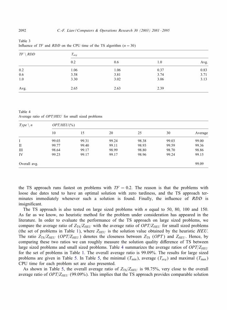
Table 3 shows the in9uence of TF and RDD on the average CPU time of the TS approach.The problem size is set at n = 30. Results for other problem sizes are similar. It is noted that


Table 3In9uence of TF and RDD on the CPU time of the TS algorithm (n = 30)

TF \ RDD Tavg

0.2 0.6 1.0 Avg.

0.2 1.06 1.06 0.37 0.830.6 3.58 3.81 3.74 3.711.0 3.30 3.02 3.06 3.13

Avg. 2.65 2.63 2.39

Table 4Average ratio of OPT=HEU for small sized problems

Type \ n OPT=HEU (%)

10 15 20 25 30 Average

I 99.03 99.31 99.24 98.38 99.03 99.00II 99.77 99.40 99.11 98.93 99.59 99.36III 98.64 99.17 98.99 98.80 98.70 98.86IV 99.23 99.17 99.17 98.96 99.24 99.15

Overall avg. 99.09

the TS approach runs fastest on problems with TF = 0:2. The reason is that the problems withloose due dates tend to have an optimal solution with zero tardiness, and the TS approach ter-minates immediately whenever such a solution is found. Finally, the in9uence of RDD isinsigni4cant.

The TS approach is also tested on large sized problems with n equal to 50, 80, 100 and 150.As far as we know, no heuristic method for the problem under consideration has appeared in theliterature. In order to evaluate the performance of the TS approach on large sized problems, wecompare the average ratio of ZTS=ZHEU with the average ratio of OPT=ZHEU for small sized problems(the set of problems in Table 1), where ZHEU is the solution value obtained by the heuristic HEU.The ratio ZTS=ZHEU (OPT=ZHEU ) denotes the closeness between ZTS (OPT ) and ZHEU . Hence, bycomparing these two ratios we can roughly measure the solution quality di;erence of TS betweenlarge sized problems and small sized problems. Table 4 summarizes the average ratios of OPT=ZHEU

for the set of problems in Table 1. The overall average ratio is 99.09%. The results for large sizedproblems are given in Table 5. In Table 5, the minimal (Tmin), average (Tavg) and maximal (Tmax)CPU time for each problem set are also presented.

As shown in Table 5, the overall average ratio of ZTS=ZHEU is 98.75%, very close to the overallaverage ratio of OPT=ZHEU (99.09%). This implies that the TS approach provides comparable solution


Table 5Performance of TS approach for large sized problems

Type n Tmin Tavg Tmax ZTS=HEU (%)

I 50 0.00 13.50 21.76 98.6880 0.00 49.19 81.13 98.88

100 0.00 95.68 160.66 98.20150 0.00 304.66 512.82 98.72

II 50 0.00 8.51 16.93 98.8880 0.00 35.06 60.41 98.80

100 0.00 66.42 121.57 98.97150 0.00 216.08 374.78 99.25

III 50 0.00 14.25 22.05 98.4080 0.00 53.76 82.69 98.61

100 0.00 100.21 158.33 98.42150 0.00 323.12 532.85 98.53

IV 50 0.00 9.07 16.14 99.0380 0.00 36.32 59.98 98.82

100 0.00 69.76 118.44 98.89150 0.00 223.84 393.23 98.96

Average 98.75

qualities for both small and large sized problems. The maximal CPU time for a problem with n=150is 532:85 s. These results show that the TS approach is capable of 4nding extremely high-qualitysolutions within a reasonable amount of time.

6. Conclusions

In this article, the problem of scheduling two-machine preemptive open shops to minimize totaltardiness is examined. An optimal timing algorithm is presented to determine the optimal schedule fora given job completion sequence. A TS approach is proposed to search for an optimal or near-optimaljob completion sequence. The TS approach employs an alternating neighborhood structure and adynamic TL scheme. Intensi4cation and diversi4cation strategies are also developed to improve theperformance of the TS approach. Computational experiments based on randomly generated problemswith various sizes show that the proposed TS approach provides excellent results. For small sizedproblems, the TS approach 4nds optimal solutions in 98.56% of the cases. For those problems thatare not solved optimally the maximal deviation from the optimal value is 1.82%. The TS approachalso provides extremely high-quality solutions for large sized problems within a reasonable amountof time. The results of our experiments indicate that the proposed TS approach is very e;ective ande#cient in solving the two-machine preemptive open shop problem with the objective of minimizingtardiness.


References

[1] Brucker P. Scheduling algorithms. Berlin Heidelberg: Springer, 1995.[2] Pinedo M. Scheduling: theory, algorithms, and systems. Englewood Cli;s, NJ: Prentice Hall, 1995.[3] Graham RL, Lawler EL, Lenstra JK, Rinnooy Kan AHG. Optimization and approximation in deterministic sequencing

and scheduling: a survey. Annals of Discrete Mathematics 1979;5:287–326.[4] Du J, Leung JY-T. Minimizing total tardiness on one machine is NP-hard. Mathematics of Operations Research

1990;15:483–95.[5] Achugbue JO, Chin FY. Scheduling the open shop to minimize mean 9ow time. SIAM Journal on Computing

1982;11:709–20.[6] Brasel H, Tautenhahn T, Werner F. Constructive heuristic algorithms for the open shop problem. Computing

1993;51:95–110.[7] Brucker P, Hurink J, Jurish B, Wostmann B. A branch and bound algorithm for the open-shop problem. Discrete

Applied Mathematics 1997;76:43–59.[8] Gueret C, Prins C. Classical and new heuristics for the open-shop problem. European Journal of Operational Research

1998;107(2):306–14.[9] Liaw CF. A hybrid genetic algorithm for the open shop scheduling problem. European Journal of Operational

Research 2000;124(1):28–42.[10] Gonzalez T, Sahni S. Open shop scheduling to minimize 4nish time. Journal of the Association for Computing

Machinery 1976;23(4):665–79.[11] Gonzalez T. A note on open shop preemptive schedules. IEEE Transactions on Computers 1979;C-28:782–6.[12] Cho Y, Sahni S. Preemptive scheduling of independent jobs with release and due times on open, 9ow and job shops.

Operations Research 1981;29:511–22.[13] Lawler EL, Lenstra JK, Rinnooy Kan AHG. Minimizing maximum lateness in a two-machine open shop. Mathematics

of Operations Research 1981;6:153–8.[14] Liu CY, Bul4n RL. On the complexity of preemptive open shop scheduling problem. Operations Research Letters

1985;4:71–4.[15] Liu CY, Bul4n RL. Scheduling ordered open shops. Computers and Operations Research 1987;14(3):257–64.[16] Liu CY. A branch-and-bound algorithm for the preemptive open shop scheduling problem. Journal of the Chinese

Institute of Industrial Engineers 1995;12(1):25–31.[17] Liaw CF. Scheduling preemptive open shops to minimize total tardiness. European Journal of Operational Research,

2001, in review.[18] Sriskandarajah C, Wagneur E. On the complexity of preemptive openshop scheduling problems. European Journal

of Operational Research 1994;77:404–14.[19] Baker KR, Bertrand J. A dynamic priority rule for scheduling against due-dates. Journal of Operations Management

1982;3:37–42.[20] Glover F. Future paths for integer programming and linkage to arti4cial intelligence. Computers and Operations

Research 1986;13:533–49.[21] Glover F. Tabu search—Part I. ORSA Journal on Computing 1989;1:190–206.[22] Glover F. Tabu search—Part II. ORSA Journal on Computing 1990;2:4–32.[23] Glover F, Laguna M. Tabu search. Dordrecht: Kluwer Academic Publishers, 1997.[24] Rayward-Smith VJ, Osman IH, Reeves CR, Smith GD, editors. Modern heuristic search methods. Chichester: Wiley,

1996.[25] Reeves CR, editor. Modern heuristic techniques for combinatorial problems. Oxford: Blackwell Scienti4c Publications,

1993.[26] Chakrapani J, Skorin-Kapov J. Massively parallel tabu search for quadratic assignment problem. Annals of Operations

Research 1993;41:327–41.[27] Dell’Amico M, Trubian M. Applying tabu search to the job-shop scheduling problem. Annals of Operations Research

1993;41:231–52.[28] Taillard E. Robust taboo search for the quadratic assignment problem. Parallel Computing 1991;17:443–55.[29] Xu J, Chiu SY, Glover F. Fine-tuning a tabu search algorithm with statistical tests. International Transactions on

Operational Research 1998;5(3):233–44.


[30] Lageweg BJ, Lenstra JK, Rinnooy Kan AHG. A general bounding scheme for the permutation 9ow-shop problem.Operations Research 1978;26:53–67.

[31] Fisher ML. A dual algorithm for the one machine scheduling problem. Mathematical Programming 1976;11:229–51.

Ching-Fang Liaw received B.B.A. and M.S. degrees in Industrial Management from National Cheng Kung University,Taiwan, and a Ph.D. degree in Industrial and Operation Engineering from the University of Michigan, MI. He is currentlya Professor at the Chaoyang University of Technology, Taiwan. His research interests include combinatorial optimizationand heuristic search methods with applications to production scheduling, and vehicle routing and scheduling.

an efficient tabu search approach for the two-machine preemptive open shop scheduling problem

Documents