1

An Efficient Scheme of Static Hedging Barrier Options: Richardson Extrapolation Techniques

Jia-Hau Guo*, Lung-Fu Chang **

December, 2016

ABSTRACT

We propose an accelerated static replication approach for pricing barrier options by employing

repeated Richardson extrapolation techniques. This approach could significantly improve the

computational efficiency and accuracy of static hedging barrier options. This approach also

provides a reliable error estimation method that aids to determine how many replication matched

points should be considered for attaining to a given desired accuracy. This approach is first

applied for barrier options under the model of Derman, Ergener, and Kani (1995) and then its

application is further extended to the model of Fink (2003). Numerical results demonstrate that

there is a significant reduction of error in percentage after employing our approach especially

when there are only a few time points matched in static hedging.

JEL Classification: G13

Keywords：Barrier option pricing; Static hedging; Richardson extrapolation technique; Error estimation; Romberg sequence

* Guo is from the Department of Information Management and Finance, College of Management, National Chiao Tung University, Hsinchu, Taiwan. ** Chang is from the Department of Finance, National Taipei University of Business, Taipei, Taiwan. Correspondence to: Professor Jia-Hau Guo, College of Management, National Chiao Tung University, No. 1001, Ta-Hsueh Rd., Hsinchu 300, Taiwan. Tel:+886-3-5712121#57078 Fax:+886-3-5733260 E-mail: jiahau@faculty.nctu.edu.tw

2

1. Introduction

Hedging exotic options is an important work for the financial institutions to manage risks. The

static hedge and the dynamic hedge approaches are two main hedging methods in the financial

literature. Compared with the dynamic hedging approach, the static hedge may be cheaper when

the transaction frequency is high and the transaction cost is large. There two categories of static

hedging approaches developed. The first approach, proposed by Bowie and Carr (1994), Carr

and Chou (1997), and Carr, Ellis, and Gupta (1998), is to construct static replication portfolio in a

continuum of standard European options with the same maturity as the exotic option but different

strike prices. The second approach, developed by Derman, Ergener, and Kani (DEK, 1995)

utilize a standard European option to match the boundary at maturity of the exotic option and a

continuum of standard European options with the same strike price but different maturities to

match the boundary before the maturity of the exotic option. Chung, Shih, and Tsai (2010) show

the modified DEK model improving performance of the static hedging method for barrier options

significantly. The replication errors of the DEK model results from the non-zero value of the

static replication portfolio on the barrier except at some discrete time points. It is able to increase

the number of time points to enhance the accuracy of static hedging. However, increasing the

number of time points will result in computationally time consuming. In this paper, we employ a

new method to improve the efficiency of static hedging in the second category and focus on

barrier options for illustration. Pricing and hedging Barrier options is a major topic in the

financial research. For example, Heynen and Kat (1996) derive the formulae for a series of

special types of barrier options. Ndogmo and Ntwiga (2011) apply a high-order accurate implicit

method to price barrier options.

Richardson extrapolation technique is often employed to derive an efficient computational

formula for evaluating the values of options. For example, Geske and Johnson (1984) firstly use

3

Richardson extrapolation technique to price compound options. Chang, Chung, and Stapleton

(2007) also use Richardson extrapolation technique to price American-style options. Chang, Guo,

and Hung (2016) further employ Richardson extrapolation technique to derive a more general and

computationally efficient formula for American options. However, while Richardson

extrapolation technique succeeds in deriving efficient approximation formulae for options, its

application in static hedging is seldom explored. Because the computationally time consuming

problem of static hedging, it is nature and important to utilize the Richardson extrapolation

technique to enhance its computational efficiency and accuracy. Employing Richardson

extrapolation technique to derive an approximation may also provide a way to determine the

accuracy of the approximation.1 One question is how many options or time points we have to

choose to achieve a given level of accuracy. Farago, Havasi, and Zlatev (2010) give a reliable

error estimation method by applying Richardson extrapolation. We employ the method proposed

by Farago, Havasi, and Zlatev (2010) to determine the number of matched replication points or

options that should be included into a static replication portfolio to achieve a given desired

replication accuracy.

In this paper, we provide a general accelerated static replication approach with the repeated

Richardson extrapolation for pricing barrier options. This article provides an error estimation

method to obtain the appropriate number of matched replication points given an error tolerance

level. The rest of this paper is organized as follow: In the second section, we introduce the

repeated Richardson extrapolation technique. Section 3 shows a basic model for illustration and

its numerical results. In Section 4, we describe the error estimation method. Section 5 provides an

1 Ibanez (2002) obtains the correct order for the error term by applying the Richardson extrapolation for pricing American option. Chang, Chung, and Stapleton (2007) also use Richardson extrapolation technique to provide reliable error estimation for pricing American-style options.

4

extension of Richardson extrapolation technique in static replication to Heston’s stochastic

volatility model. Finally, the conclusion is given in section 6.

2. Repeated-Richardson Extrapolation

The Richardson extrapolation is a powerful technique to improve the accuracy of estimations.

Consider an unknown quantity 𝑓(0) as the exact value that is approximated by a monotonous

function 𝑓(ℎ). The parameter ℎ > 0 so that we have limℎ→0 𝑓(ℎ) = 𝑓(0) = 𝑎0 . We can

perform the repeated Richardson extrapolation technique to approximate the unknown value 𝑎0.

Assume that

𝑓(ℎ) = 𝑎0 + 𝑎1ℎ𝑝1 + 𝑎2ℎ𝑝2 + 𝑎3ℎ𝑝3 + ⋯+ 𝑎𝑘ℎ𝑝𝑘 + Ο(ℎ𝑝𝑘+1) (1)

For 𝑎𝑖, (𝑖 = 1, 2, 3,⋯ ,𝑘) is unknown and 𝑝1 < 𝑝2 < 𝑝3 < ⋯ < 𝑝𝑘 < 𝑝𝑘+1, where Ο(ℎ𝑝𝑘+1)

denotes a quantity whose size is proportional to ℎ𝑝𝑘+1 . Specially, we assume that limℎ→0 𝑓(ℎ) =

𝑓(0) = 𝑎0 when the step size goes to zero ( ℎ = 0). The idea of the Richardson extrapolation is

that we can find a linear combination of two different step sizes. For the sequence of the

estimation: 𝑓(ℎ1) , 𝑓(ℎ2),⋯ ,𝑓(ℎ𝑛) , we define 𝑓𝑖,1 = 𝑓(ℎ𝑖) , for 𝑖 = 1, 2, 3,⋯ , 𝑛. . For 𝑗 =

2, 3, 4,⋯ , 𝑖, the Richardson extrapolation and its repeated version are defined by

𝑓𝑖,𝑗 = 𝑓𝑖+1,𝑗−1 + 𝑓𝑖+1,𝑗−1−𝑓𝑖,𝑗−1

� ℎ𝑖ℎ𝑖+1

�𝑝−1

. (2)

The computation can be set up as follows:

𝑓(ℎ1) = 𝑓1,1 𝑓1,2 𝑓1,3 𝑓1,4 ⋯ 𝑓1,𝑛

𝑓(ℎ2) = 𝑓2,1 𝑓2,2 𝑓2,3

𝑓(ℎ3) = 𝑓3,1 𝑓3,2

𝑓(ℎ4) = 𝑓4,1

5

The repeated Richardson extrapolation technique avoids complicated calculation and provides a

better result of estimation. Therefore, the repeated Richardson extrapolation can be used to

enhance the computational efficiency and accuracy of the static hedging.

3. Basic Model and Numerical Results

In this section, the well-known Black-Scholes model is considered to be a basic model for the

illustration of how to employ Richardson extrapolation technique to improve the efficiency and

accuracy of static hedging barrier options. One reason for the Black-Scholes model is that the

existing analytical formulae of barrier options can be treated as benchmarks. The basic model

under the risk-neutral measure is given by

𝑑𝑆𝑡 = (𝑟 − 𝑑)𝑆𝑡𝑑𝑑 + 𝜎𝑆𝑡𝑑𝑊𝑡, (3)

where 𝑆𝑡 is the stock price at time 𝑑, 𝑟 is the risk-free interest rate, 𝑑 is the dividend yield, 𝜎 is the

volatility, and 𝑊𝑡 denotes a Wiener process.

To solve the possible problem of nonuniform convergence, Omberg (1987) and Chang,

Chung, and Stapleton (2007) suggest using geometric-spaced exercise points generated by

successively doubling the number of uniformly-spaced exercise dates. Therefore, we also employ

Romberg sequence to implement the repeated Richardson extrapolation technique. Romberg

sequence: {1, 2, 4, 8, 16, 32, 64, 128, . . ., 2𝑛}. One reason for Romberg sequence is to

increase the possibility that 𝑓(ℎ) could monotonically converge to 𝑓(0) by ensuring each

matched replication set nesting the previous one. In addition to Romberg sequence, we also

consider other three sequences: harmonic sequence: {1, 2, 3, 4, 5, 6, 7, 8, ⋯ , 𝑛 , ⋯}; double

⋮

𝑓(ℎ𝑛) = 𝑓𝑛,1

6

harmonic sequence: {2, 4, 6, 8, 10, 12, 14, 16, ⋯ , 2𝑛 , ⋯ }; Burlisch sequence: {2, 3, 4, 6, 8, 12,

16, 24, 32, ⋯, 2𝑛 𝑘−2 , ⋯ }. Figure 1 shows the price convergence of a standard up and out

barrier call option under the DEK model with four different sequences respectively, including

harmonic sequence, double harmonic sequence, Burlisch sequence, and Romberg sequence.

[Figure 1 is here]

All the above sequences show the uniform price convergence as the number of replication

matched time points 𝑁 increases under the DEK model. In our study, the geometric-spaced

replication matched points (i.e. Romberg sequence) and the arithmetic-spaced replication

matched points (i.e. harmonic sequence) for pricing barrier options are not necessary incurring

the problem of non-uniform convergence.2

[Table 1 is here]

However, the convergence speed of four different sequences may be quite different (see

Table 1). For a large error tolerance level, TOL=10%, the convergence speeds of four sequences

are not different from each other very much. As the error tolerance level being smaller, the

harmonic sequence and the double harmonic sequences could become markedly computational

time consuming. The computation time for the harmonic sequence could be approximately 110

times longer than that for Romberg sequence. Because the computation time of geometric-spaced

replication matched points could be much less than that of the arithmetic-spaced replication

matched points, we adopt Romberg sequence when employing repeated Richardson extrapolation

technique in static hedging barrier options. Hence, given a specific step size ℎ𝑖 = 𝑇 2𝑖−1⁄ where

𝑇 is the time to maturity of the barrier option, let 𝑓𝑖,𝑗 denote its corresponding estimation value

2 Chang, Chuang and Stapleton (2007) find that exercise points of harmonic sequence may cause non-uniform price convergence for some American-style options and incur an efficiency reduction of Richardson extrapolation technique.

7

under the DEK model. Table 2 indicates results after employing repeated Richardson

extrapolation technique in the DEK model of static hedging a standard up and out barrier call

option with model parameters as follows: current stock price 𝑆0 = 105, strike price 𝐾 = 100,

risk-free interest rate 𝑟 = 0.055, dividend yield 𝑑 = 0.025, barrier 𝐵 = 110, volatility 𝜎 = 0.2,

and time to maturity 𝑇 = 1. The benchmark value for this barrier option is 0.0611 derived from

the existing analytical formula under the Black-Scholes model.

[Table 2 is here]

Table 2 shows that repeated Richardson extrapolation technique could provide more efficient and

accurate estimators for static hedging barrier options under the DEK model.

4. Error Estimation

The advantage of the repeated Richardson extrapolation technique is that we are able to acquire

the error bounds of the approximation. The repeated Richardson extrapolation can determine the

accuracy of the approximation and how many replication matched points should be considered

for attaining to a given desired accuracy. Therefore, the repeated Richardson extrapolation

provides a useful method to improve the accuracy of the static replication method for pricing

barrier options. Moreover, Farago, Havasi, and Zlatev (2010) show that the error of estimation

based on the Richardson extrapolation method can be calculated by ERROR = �𝜔𝑛−𝑍𝑛2𝑝−1

�, where 𝜔𝑛

and 𝑍𝑛 are estimators and 𝑍𝑛 has the double step size of 𝜔𝑛 . The estimation value for the

specific step size h is given by:

𝑍𝑛 = 𝑓(ℎ) = 𝑎0 + 𝑎1ℎ𝑝1 + Ο(ℎ𝑝2) (4)

For choosing another step size,

𝜔𝑛 = 𝑓 �ℎ2� = 𝑎0 + 𝑎1(ℎ

2)𝑝1 + Ο(ℎ𝑝2) (5)

8

By omitting the high order term and eliminating 𝑎0, we are able to obtain

𝑎1 =2𝑝1(𝑓�ℎ2�−𝑓(ℎ))

ℎ𝑝1(2𝑝1−1) (6)

and substitute Eq. (6) into Eq. (5)

𝑓 �ℎ2� − 𝑎0 =

𝑓�ℎ2�−𝑓(ℎ)

2𝑝1−1+ Ο(ℎ𝑝2) (7)

The left side denotes the accurate error and the right side represents an estimation error.

Based on the method of Farago, Havasi, and Zlatev (2010), we define the estimated error by

|𝑓𝑖+1,𝑗−𝑓𝑖,𝑗| and the accurate error is |𝑓𝑖+1,𝑗 − 𝑎0|, where 𝑎0 is the theoretical value of the barrier

option and (𝑝1,𝑝2) = (1,2) denotes the Richardson extrapolation of two adjacent points. We are

able to show how the step size can be chosen to meet the error tolerance level in advance.

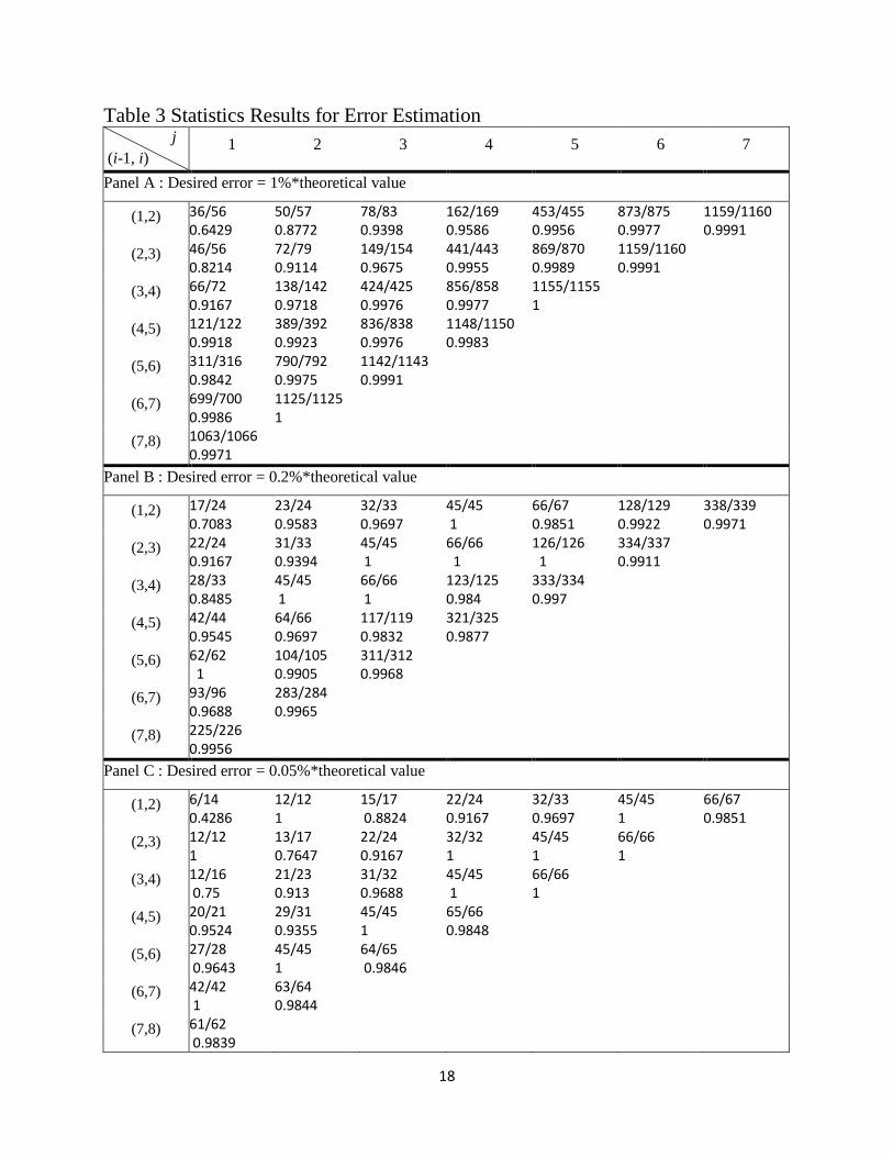
[Table 3 is here]

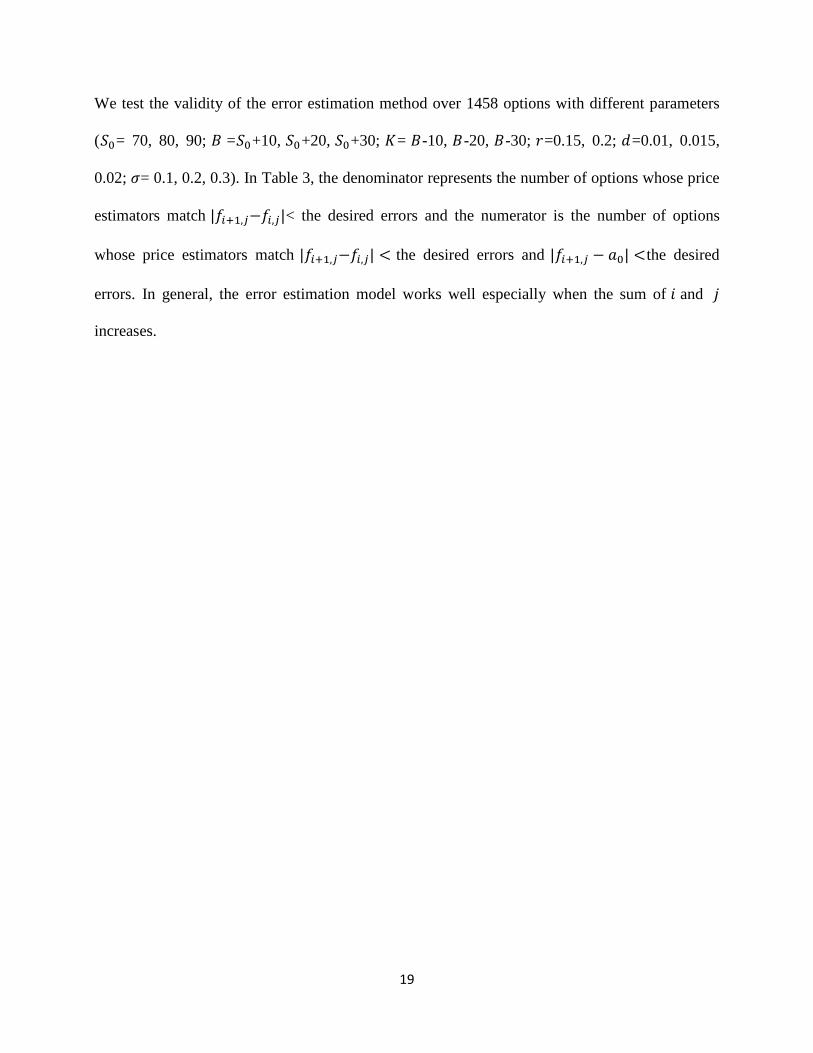
The validity of the error estimation method may depend on the high order term Ο(ℎ2). We

test the validity of our error estimation method over 1458 options with different parameters (𝑆0=

70, 80, 90; 𝐵 =𝑆0+10, 𝑆0+20, 𝑆0+30; 𝐾= 𝐵-10, 𝐵-20, 𝐵-30; 𝑟=0.15, 0.2; 𝑑=0.01, 0.015, 0.02; 𝜎=

0.1, 0.2, 0.3). The numerical testing results can be shown in Table 3. In Table 3, the denominator

represents the number of options whose price estimators match |𝑓𝑖+1,𝑗−𝑓𝑖,𝑗|< the desired errors

and the numerator is the number of options whose price estimators match |𝑓𝑖+1,𝑗−𝑓𝑖,𝑗| < the

desired errors and |𝑓𝑖+1,𝑗 − 𝑎0| <the desired errors. In general, the error estimation model works

well especially when the sum of 𝑖 and 𝑗 increases. This finding is consistent with the result of

Chang, Chuang and Richard (2007), who utilize the Schmidt inequality (1968). For example,

when (𝑖, 𝑖 − 1) = (3, 4) and 𝑗 =3, there are 424 options out of 425 options which satisfy the actual

error less than the desired error (1% of the theoretical value) given the estimation error less than

the desired error. Hence, the probability of estimates satisfying the required accuracy is more

9

than 99 percent. Therefore, we can further provide a quite accurate estimator of the number of

options which would be used to consist of the static hedging portfolio to achieve the required

replication accuracy.

On the other hand, it is nature to control the step size of the repeated Richardson

extrapolation given an error tolerance parameter that makes the estimation error meet our

requirement. Farago, Havasi, and Zlatev (2010) suggest a step size control method which is given

by

ℎ𝑛𝑛𝑛 = 𝜔 × � 𝑇𝑇𝑇𝐸𝐸𝐸𝑇𝐸

𝑝ℎ𝑜𝑜𝑜 (8)

where ω = 0.9 in experimental practices, p=1, and

ℎ𝑛 = 𝑇2𝑛−1� . (9)

Substituting h from Eq. (9) into Eq. (8) ,

𝑛𝑛𝑛𝑛 = 𝑛𝑜𝑜𝑜 + 𝐿𝐿𝐿2 �𝐸𝐸𝐸𝑇𝐸𝑇𝑇𝑇

� − 𝐿𝐿𝐿2(𝜔) . (10)

Given a specific error tolerance level (TOL) and the initial value of 𝑛𝑜𝑜𝑜, we could obtain a better

estimator of 𝑛𝑛𝑛𝑛 to achieve the required accuracy based on Eq. (10). However, the computation

time of finding the best step size may be time consuming if an improper initial parameter (𝑛) is

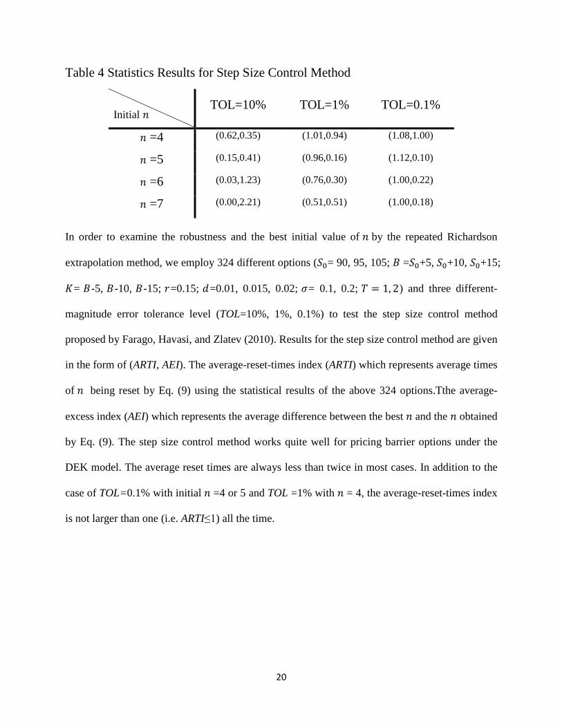
used. In order to examine the robustness and the best initial value of 𝑛 by the repeated

Richardson extrapolation method, we employ 324 different options (𝑆0= 90, 95, 105; 𝐵 =𝑆0+5,

𝑆0+10, 𝑆0+15; 𝐾= 𝐵-5, 𝐵-10, 𝐵-15; 𝑟=0.15; 𝑑=0.01, 0.015, 0.02; 𝜎= 0.1, 0.2; 𝑇 = 1, 2) and three

different-magnitude error tolerance level (TOL=10%, 1%, and 0.1%) to test the step size control

method proposed by Farago, Havasi, and Zlatev (2010).

[Table 4 is here]

We develop two measurement indexes as follows. One is the average-reset-times index

(ARTI) which represents average times of 𝑛 being reset by Eq. (10) using the statistical results of

10

the above 324 options. Given a proper initial 𝑛𝑜𝑜𝑜 , the best situation is that the step size control

method of Farago, Havasi, and Zlatev (2010) always finds the best 𝑛𝑛𝑛𝑛 at the first time and

ARTI will be one. The other measurement index is the average-excess index (AEI) which

represents the average difference between the best 𝑛 and the 𝑛 obtained by Eq. (10). The

implication of AEI is to show how much resource is wasted to calculate an overestimated 𝑛.

Under the optimization situation, the parameter AEI should be zero. For example, in case of

pricing the up and out barrier call option mentioned above with a required TOL = 1% and

specifying initial value of 𝑛 =5. Based on Eq. (10), we obtain the new 𝑛 = 8 and the

corresponding error = 0.36%. But the best 𝑛 is 7 with the error =0.76%. In this numerical

example, the variable 𝑛 is reset once, and the difference between the 𝑛 computed by Eq. (10) and

the best 𝑛 is 8-7 = 1. Hence, the index ARTI is 1 and AEI is also 1.

The statistical results of the above 324 options have been shown in Table 4. In these

numerical results, the step size control method of Farago, Havasi, and Zlatev (2010) works quite

well for pricing barrier options under the DEK model. The average reset times are always less

than twice in most cases. In addition to the case of TOL=0.1% with initial 𝑛 =4 or 5 and TOL

=1% with 𝑛 = 4, the average-reset-times index is not larger than one (i.e. ARTI≤1) all the time.

This finding supports that we are able to obtain a proper 𝑛 by applying the step size control

method with a given error tolerance level. Based on the results of Table 4, we can choose a

proper initial 𝑛 for a required error tolerance level. For the TOL=10%, 1%, and 0.1%, the best

initial 𝑛 are those with the lowest sum of ARTI and AEI which are 𝑛 =5, 5, and 7.

5. An Extension to Heston’s Stochastic Volatility Model

We assume that the stochastic process that drives the price of the underlying asset is given by

𝑑𝑆𝑡 = (𝑟 − 𝑑)𝑆𝑡𝑑𝑑 + �𝑉𝑡𝑆𝑡(𝜌𝑑𝑊𝑡𝑉 + �1 − 𝜌2𝑑𝑊𝑡

𝑆), (11)

11

𝑑𝑉𝑡 = 𝜅(𝜃 − 𝑉𝑡)𝑑𝑑 + 𝜎�𝑉𝑡𝑑𝑊𝑡𝑉, (12)

where 𝜅 determines the rate of mean reversion of the variance, 𝜃 is its long run mean, and 𝜎

determines the volatility of the variance. 𝜎 is often referred to as “volatility of volatility.” 𝑊𝑡𝑉

and 𝑊𝑡𝑆 are independent Wiener processes. Heston (1993) derives a semi-analytical formula for

the value of a European call option when the stock price follows this process. Fink (2003)

construct a static hedging whose value equals that of a barrier option for a set of points along the

boundary for not just one volatility state, but for a set of volatility states. As before, to create a

static hedging we require a portfolio that is equal in value to the up and out call at all points both

on the barrier and at the terminal date. One may approximate such a hedge by matching not only

at 𝑛 different points in time, but also at each of 𝑛𝑉 different volatility states. The approach is to

construct a portfolio equal in value to the up and out call on the grid of points and having no

payoff in the interior.

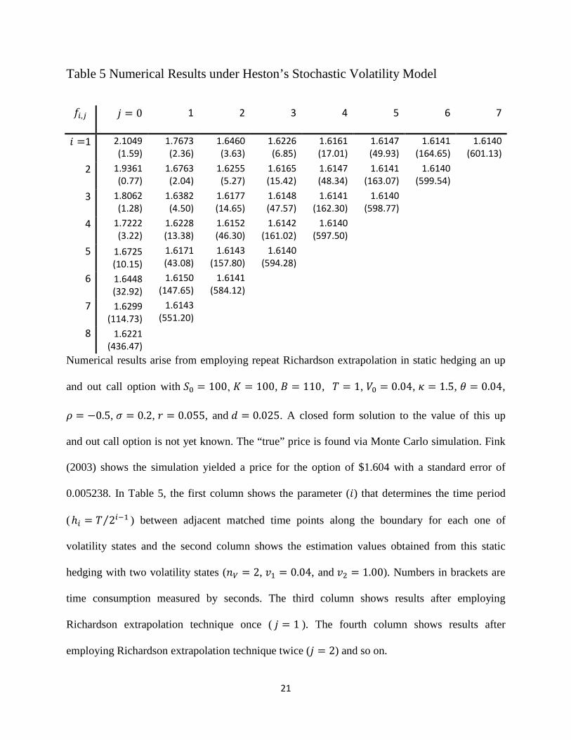
[Table 5 is here]

Assume that the underlying price follows model of (11) and (12) with 𝑉0 = 0.04, 𝜅 = 1.5,

𝜃 = 0.04, 𝜌 = −0.5, 𝜎 = 0.2, 𝑟 = 0.055, and 𝑑 = 0.025. A closed form solution to the value of

an up and out call option with 𝑆0 = 100, 𝐾 = 100, 𝐵 = 110, and 𝑇 = 1 is not yet known. The

“true” price is found via Monte Carlo simulation. Fink (2003) shows the simulation yielded a

price for the option of $1.604 with a standard error of 0.005238. In Table 5, the first column

shows the parameter (𝑖) that determines the time period (ℎ𝑖 = 𝑇 2𝑖−1⁄ ) between adjacent matched

time points along the boundary for each one of volatility states and the second column shows the

estimation values obtained from this static hedging with two volatility states (𝑛𝑉 = 2, 𝑣1 = 0.04,

and 𝑣2 = 1.00). Numbers in brackets are time consumption measured by seconds. The third

column shows results after employing Richardson extrapolation technique once (𝑗 = 1). The

12

fourth column shows results after employing Richardson extrapolation technique twice (𝑗 = 2).

The fifth column shows results after employing Richardson extrapolation technique three times

(𝑗 = 3) and so on. The benefit to employ Richardson extrapolation technique is significant

especially when there are only a few time points matched in static hedging. For example, when

𝑖 = 3, there are only 5 (5 = 23−1 + 1) matched time points along the boundary for each one of

volatility states. Applying static hedging with two volatility states gives 𝑓3,0 = 1.8062 and

𝑓2,0 = 1.9361 . After employing Richardson extrapolation once, we have 𝑓2,1 = 𝑓3,0 +

�𝑓3,0 − 𝑓2,0� (2 − 1)⁄ = 1.6763 by Eq. (2). A reduction of error in percentage is

��𝑓3,0 − 𝑎0� − �𝑓2,1 − 𝑎0�� �𝑓3,0 − 𝑎0�� = 64.24% where 𝑎0 = 1.604 . If employing Richardson

extrapolation twice, we have 𝑓1,2 = 1.6460 and a further reduction of error in percentage is

��𝑓3,0 − 𝑎0� − �𝑓1,2 − 𝑎0�� �𝑓3,0 − 𝑎0�� =79.23% with a total computation time of 3.63 seconds.

Note that 𝑓6,0 = 1.6448 provides a similar accuracy but its computation time is 32.92 seconds.

6. Conclusion

This paper proposes an accelerated static replication approach for pricing barrier options by

employing repeated Richardson extrapolation techniques. This approach is first examined for

barrier options under the model of Derman, Ergener, and Kani (1995). We employ four different

sequences including harmonic sequence, double harmonic sequence, Burlisch sequence, and

Romberg sequence to examine their convergence properties and speeds. All the above sequences

indicate the uniform convergence. However, the computational time of geometric-spaced

exercise points (Romberg sequence) is efficiently less than that of the arithmetic-spaced exercise

points (harmonic sequence). Based on the method of Farago, Havasi, and Zlatev (2010), our

proposed model can provide a reliable error estimation method and acquire the specific

replication portfolio under any given error tolerance level by utilizing the repeated Richardson

13

extrapolation technique. Numerical results demonstrate that the error estimation method works

well and aids to determine how many replication matched points should be considered for

attaining to a given desired accuracy.

Then, the application of our approach is further extended to the model of Fink (2003). We

find that there is also a significant improvement in the computational efficiency and accuracy of

static hedging barrier options. Numerical results demonstrate that there is a significant reduction

of error in percentage after employing our approach especially when there are only a few time

points matched in static hedging. A further extension of our proposed approach to other option

static hedging problems is left for future studies.

14

Reference

Black, F., Scholes, M., 1973. The pricing of options and corporate liability, Journal of Political Economy 81, 637–654.

Bowie, J., Carr, P., 1994. Static simplicity, Risk Magazine 7, 45–49.

Carr, P., Chou, A., 1997. Breaking barriers: static hedging of barrier securities, Risk Magazine 10, 139–145.

Carr, P., Ellis, K., Gupta, V., 1998. Static hedging of exotic options, Journal of Finance 3, 1165–1190.

Chang, C., Chuang, S., Stapleton, R., 2007. Richardson extrapolation techniques for the pricing of American-style options, Journal of Futures Markets 27, 791–187.

Chang, L, Guo, J., Hung, M., 2016. A generalization of the recursive integration method for the analytic valuation of American options, Journal of Futures Markets, 36, 887-901.

Chung, S., Shih, P., Tsai, W., 2010. A modified static hedging method for continuous barrier options, Journal of Futures Markets 30, 1150–1166.

Geske, R., Johnson, H., 1979. The valuation of compound options, Journal of Financial Economics 7, 63–81.

Chou, A., Georgiev, G., 1998. A uniform approach to static replication, Journal of Risk 1, 73–87.

Derman, E., Ergener, D., Kani, I., 1995. Static options replication, Journal of Derivatives 2, 78–95.

Farago, I., Havasi, A., Zlatev, Z., 2010. Efficient implementation of stable Richardson extrapolation algorithms, Computers and Mathematics with Applications 60, 2309–2325.

Fink, J., 2003. An examination of the effectiveness of static hedging in the presence of stochastic volatility, Journal of Futures Markets 23, 859–890.

Geske, R., Johnson, H., 1979. The valuation of compound options, Journal of Financial Economics 7, 63–81.

Heynen, P., Kat, H., 1996. Discrete partial barrier options with a moving barrier, Journal of Financial Engineering 5, 199–209.

Heston, S., 1993. A closed-form solution for options with stochastic volatility with application to bond and currency option. Review of Financial Studies 6, 327–343.

15

Ibanez, A., 2002. Robust pricing of the American put option: a note on Richardson extrapolation and the early exercise premium, Management Science 49, 1210–1228.

Ndogmo, J., Ntwiga, D., 2011. High-order accurate implicit methods for barrier option pricing, Applied Mathematics and Computation 218, 2210–2224.

Omberg, E., 1987. A note on the convergence of the binomial pricing and compound option models, Journal of Finance 42, 463–469.

Schmidt, J., 1968. Asymptomatic approximation: an acceleration convergence method, Numerical Mathematics 11, 53–56.

16

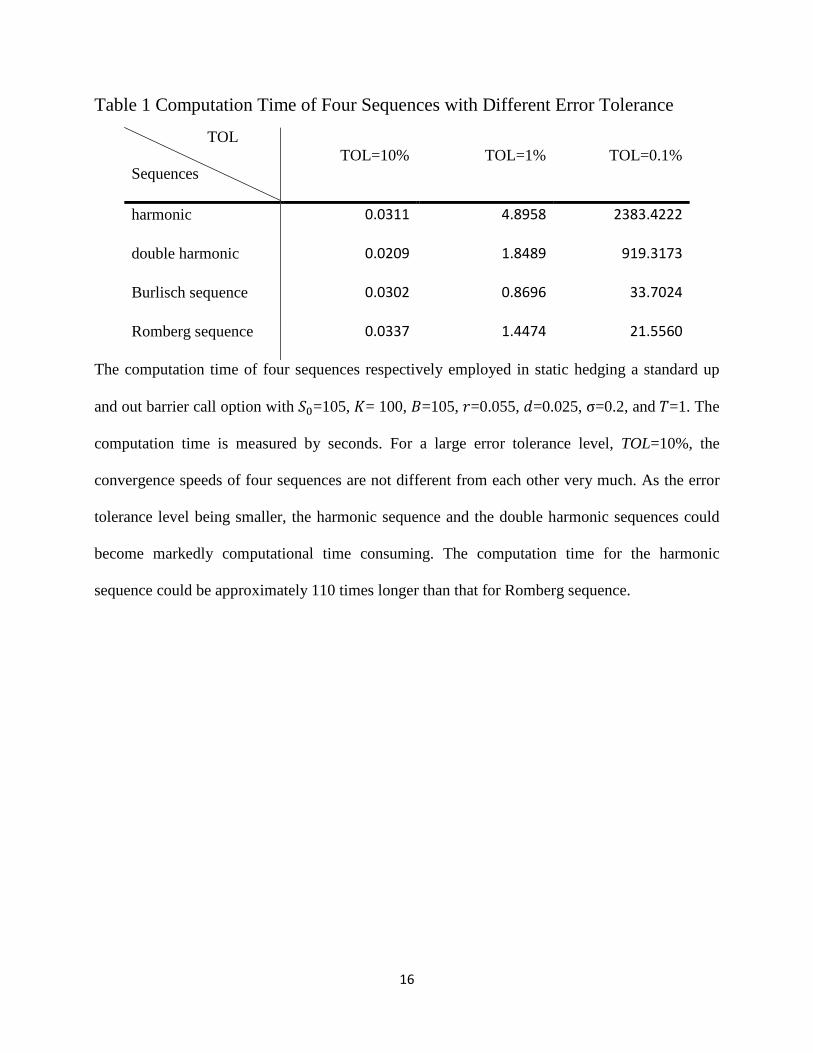
Table 1 Computation Time of Four Sequences with Different Error Tolerance

TOL

Sequences TOL=10% TOL=1% TOL=0.1%

harmonic 0.0311 4.8958 2383.4222

double harmonic 0.0209 1.8489 919.3173

Burlisch sequence 0.0302 0.8696 33.7024

Romberg sequence 0.0337 1.4474 21.5560

The computation time of four sequences respectively employed in static hedging a standard up

and out barrier call option with 𝑆0=105, 𝐾= 100, 𝐵=105, 𝑟=0.055, 𝑑=0.025, σ=0.2, and 𝑇=1. The

computation time is measured by seconds. For a large error tolerance level, TOL=10%, the

convergence speeds of four sequences are not different from each other very much. As the error

tolerance level being smaller, the harmonic sequence and the double harmonic sequences could

become markedly computational time consuming. The computation time for the harmonic

sequence could be approximately 110 times longer than that for Romberg sequence.

17

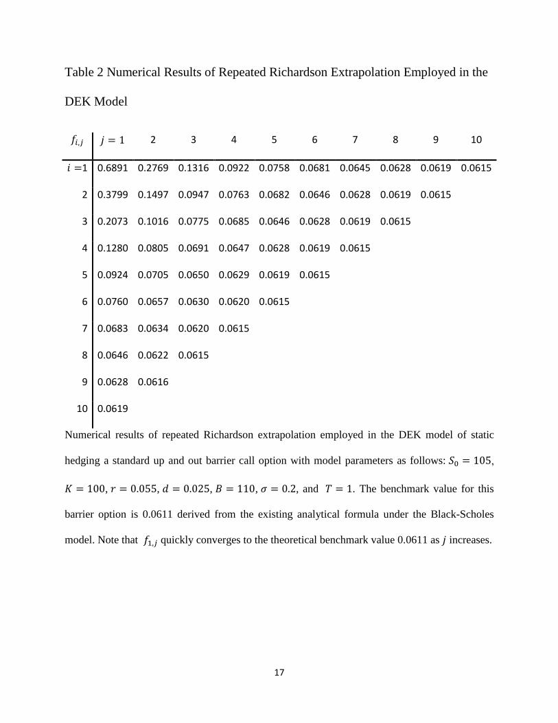
Table 2 Numerical Results of Repeated Richardson Extrapolation Employed in the

DEK Model

𝑓𝑖,𝑗 𝑗 = 1 2 3 4 5 6 7 8 9 10

𝑖 =1 0.6891 0.2769 0.1316 0.0922 0.0758 0.0681 0.0645 0.0628 0.0619 0.0615

2 0.3799 0.1497 0.0947 0.0763 0.0682 0.0646 0.0628 0.0619 0.0615

3 0.2073 0.1016 0.0775 0.0685 0.0646 0.0628 0.0619 0.0615

4 0.1280 0.0805 0.0691 0.0647 0.0628 0.0619 0.0615

5 0.0924 0.0705 0.0650 0.0629 0.0619 0.0615

6 0.0760 0.0657 0.0630 0.0620 0.0615

7 0.0683 0.0634 0.0620 0.0615

8 0.0646 0.0622 0.0615

9 0.0628 0.0616

10 0.0619

Numerical results of repeated Richardson extrapolation employed in the DEK model of static

hedging a standard up and out barrier call option with model parameters as follows: 𝑆0 = 105,

𝐾 = 100, 𝑟 = 0.055, 𝑑 = 0.025, 𝐵 = 110, 𝜎 = 0.2, and 𝑇 = 1. The benchmark value for this

barrier option is 0.0611 derived from the existing analytical formula under the Black-Scholes

model. Note that 𝑓1,𝑗 quickly converges to the theoretical benchmark value 0.0611 as 𝑗 increases.

18

Table 3 Statistics Results for Error Estimation j (i-1, i)

1 2 3 4 5 6 7

Panel A : Desired error = 1%*theoretical value

(1,2) 36/56 0.6429

50/57 0.8772

78/83 0.9398

162/169 0.9586

453/455 0.9956

873/875 0.9977

1159/1160 0.9991

(2,3) 46/56 0.8214

72/79 0.9114

149/154 0.9675

441/443 0.9955

869/870 0.9989

1159/1160 0.9991

(3,4) 66/72 0.9167

138/142 0.9718

424/425 0.9976

856/858 0.9977

1155/1155 1

(4,5) 121/122 0.9918

389/392 0.9923

836/838 0.9976

1148/1150 0.9983

(5,6) 311/316 0.9842

790/792 0.9975

1142/1143 0.9991

(6,7) 699/700 0.9986

1125/1125 1

(7,8) 1063/1066 0.9971

Panel B : Desired error = 0.2%*theoretical value

(1,2) 17/24 0.7083

23/24 0.9583

32/33 0.9697

45/45 1

66/67 0.9851

128/129 0.9922

338/339 0.9971

(2,3) 22/24 0.9167

31/33 0.9394

45/45 1

66/66 1

126/126 1

334/337 0.9911

(3,4) 28/33 0.8485

45/45 1

66/66 1

123/125 0.984

333/334 0.997

(4,5) 42/44 0.9545

64/66 0.9697

117/119 0.9832

321/325 0.9877

(5,6) 62/62 1

104/105 0.9905

311/312 0.9968

(6,7) 93/96 0.9688

283/284 0.9965

(7,8) 225/226 0.9956

Panel C : Desired error = 0.05%*theoretical value

(1,2) 6/14 0.4286

12/12 1

15/17 0.8824

22/24 0.9167

32/33 0.9697

45/45 1

66/67 0.9851

(2,3) 12/12 1

13/17 0.7647

22/24 0.9167

32/32 1

45/45 1

66/66 1

(3,4) 12/16 0.75

21/23 0.913

31/32 0.9688

45/45 1

66/66 1

(4,5) 20/21 0.9524

29/31 0.9355

45/45 1

65/66 0.9848

(5,6) 27/28 0.9643

45/45 1

64/65 0.9846

(6,7) 42/42 1

63/64 0.9844

(7,8) 61/62 0.9839

19

We test the validity of the error estimation method over 1458 options with different parameters

(𝑆0= 70, 80, 90; 𝐵 =𝑆0+10, 𝑆0+20, 𝑆0+30; 𝐾= 𝐵-10, 𝐵-20, 𝐵-30; 𝑟=0.15, 0.2; 𝑑=0.01, 0.015,

0.02; 𝜎= 0.1, 0.2, 0.3). In Table 3, the denominator represents the number of options whose price

estimators match |𝑓𝑖+1,𝑗−𝑓𝑖,𝑗|< the desired errors and the numerator is the number of options

whose price estimators match |𝑓𝑖+1,𝑗−𝑓𝑖,𝑗| < the desired errors and |𝑓𝑖+1,𝑗 − 𝑎0| <the desired

errors. In general, the error estimation model works well especially when the sum of 𝑖 and 𝑗

increases.

20

Table 4 Statistics Results for Step Size Control Method

Initial 𝑛 TOL=10% TOL=1% TOL=0.1%

𝑛 =4 (0.62,0.35) (1.01,0.94) (1.08,1.00)

𝑛 =5 (0.15,0.41) (0.96,0.16) (1.12,0.10)

𝑛 =6 (0.03,1.23) (0.76,0.30) (1.00,0.22)

𝑛 =7 (0.00,2.21) (0.51,0.51) (1.00,0.18)

In order to examine the robustness and the best initial value of 𝑛 by the repeated Richardson

extrapolation method, we employ 324 different options (𝑆0= 90, 95, 105; 𝐵 =𝑆0+5, 𝑆0+10, 𝑆0+15;

𝐾= 𝐵-5, 𝐵-10, 𝐵-15; 𝑟=0.15; 𝑑=0.01, 0.015, 0.02; 𝜎= 0.1, 0.2; 𝑇 = 1, 2) and three different-

magnitude error tolerance level (TOL=10%, 1%, 0.1%) to test the step size control method

proposed by Farago, Havasi, and Zlatev (2010). Results for the step size control method are given

in the form of (ARTI, AEI). The average-reset-times index (ARTI) which represents average times

of 𝑛 being reset by Eq. (9) using the statistical results of the above 324 options.Tthe average-

excess index (AEI) which represents the average difference between the best 𝑛 and the 𝑛 obtained

by Eq. (9). The step size control method works quite well for pricing barrier options under the

DEK model. The average reset times are always less than twice in most cases. In addition to the

case of TOL=0.1% with initial 𝑛 =4 or 5 and TOL =1% with 𝑛 = 4, the average-reset-times index

is not larger than one (i.e. ARTI≤1) all the time.

21

Table 5 Numerical Results under Heston’s Stochastic Volatility Model

𝑓𝑖,𝑗 𝑗 = 0 1 2 3 4 5 6 7

𝑖 =1 2.1049 (1.59)

1.7673 (2.36)

1.6460 (3.63)

1.6226 (6.85)

1.6161 (17.01)

1.6147 (49.93)

1.6141 (164.65)

1.6140 (601.13)

2 1.9361 (0.77)

1.6763 (2.04)

1.6255 (5.27)

1.6165 (15.42)

1.6147 (48.34)

1.6141 (163.07)

1.6140 (599.54)

3 1.8062 (1.28)

1.6382 (4.50)

1.6177 (14.65)

1.6148 (47.57)

1.6141 (162.30)

1.6140 (598.77)

4 1.7222 (3.22)

1.6228 (13.38)

1.6152 (46.30)

1.6142 (161.02)

1.6140 (597.50)

5 1.6725 (10.15)

1.6171 (43.08)

1.6143 (157.80)

1.6140 (594.28)

6 1.6448 (32.92)

1.6150 (147.65)

1.6141 (584.12)

7 1.6299 (114.73)

1.6143 (551.20)

8 1.6221 (436.47)

Numerical results arise from employing repeat Richardson extrapolation in static hedging an up

and out call option with 𝑆0 = 100, 𝐾 = 100, 𝐵 = 110, 𝑇 = 1, 𝑉0 = 0.04, 𝜅 = 1.5, 𝜃 = 0.04,

𝜌 = −0.5, 𝜎 = 0.2, 𝑟 = 0.055, and 𝑑 = 0.025. A closed form solution to the value of this up

and out call option is not yet known. The “true” price is found via Monte Carlo simulation. Fink

(2003) shows the simulation yielded a price for the option of $1.604 with a standard error of

0.005238. In Table 5, the first column shows the parameter (𝑖) that determines the time period

(ℎ𝑖 = 𝑇 2𝑖−1⁄ ) between adjacent matched time points along the boundary for each one of

volatility states and the second column shows the estimation values obtained from this static

hedging with two volatility states (𝑛𝑉 = 2, 𝑣1 = 0.04, and 𝑣2 = 1.00). Numbers in brackets are

time consumption measured by seconds. The third column shows results after employing

Richardson extrapolation technique once ( 𝑗 = 1 ). The fourth column shows results after

employing Richardson extrapolation technique twice (𝑗 = 2) and so on.

22

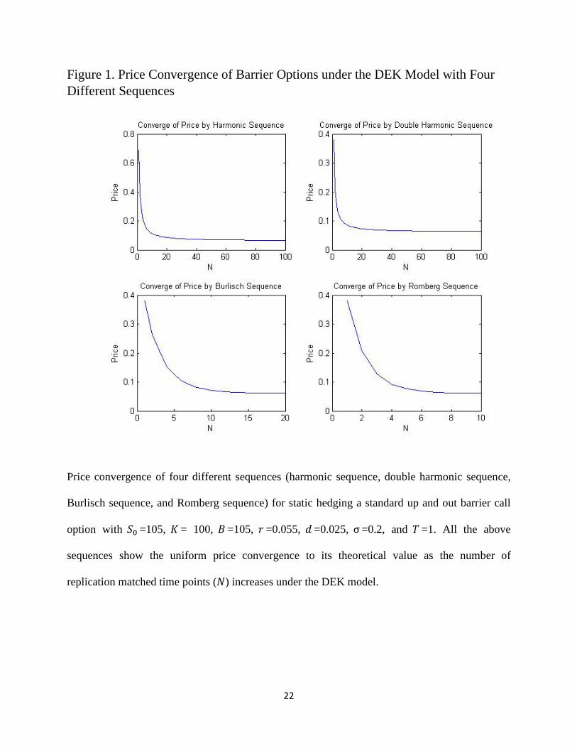
Figure 1. Price Convergence of Barrier Options under the DEK Model with Four Different Sequences

Price convergence of four different sequences (harmonic sequence, double harmonic sequence,

Burlisch sequence, and Romberg sequence) for static hedging a standard up and out barrier call

option with 𝑆0 =105, 𝐾 = 100, 𝐵 =105, 𝑟 =0.055, 𝑑 =0.025, σ=0.2, and 𝑇 =1. All the above

sequences show the uniform price convergence to its theoretical value as the number of

replication matched time points (𝑁) increases under the DEK model.