an ecological model for the management of natural … ecological model for barama, guyana. draft ii...

Centre for the Study of Environmental Change and Sustainability (CECS) The University of Edinburgh John Muir Building Mayfield Road Edinburgh EH9 3JK United Kingdom Tel: +44 131 650 7860 Fax: +44 131 650 7863 Email: [email protected] http://www.symfor.org/technical

This publication is an output from a project funded through the Forestry Research Programme of the UK Department for International Development (DFID) for the benefit of developing countries. The views expressed are not necessarily those of DFID. R6915 Forestry Research Programme.

An ecological model for the management of natural forests derived from the Barama Company

Limited plots in NW Guyana

P.D. Phillips M.T. Khan

Jagdesh Singh P.R. van Gardingen

2002

The ecological model for Barama, Guyana. DRAFT ii

Summary An ecological model describing the processes of growth, recruitment and mortality was developed using a dataset from permanent and experimental sample plots established by Barama Company Limited in NW Guyana. The model was implemented in the SYMFOR framework and calibrated and tested with simulations of primary forest dynamics.

This document describes the data and development of the model, including species groups and the sub models for growth, recruitment and mortality. These were integrated within the SYMFOR framework for evaluation and application. Results of typical simulations are presented as to enable assessment of the performance of the model.

The model was developed on the same bases as was used for the Pibiri region in Guyana.

The full text of this document is available from http://www.symfor.org/technical/barama.pdf.

The ecological model for Barama, Guyana. DRAFT iii

Contents

Summary.................................................................................................................... ii

Contents.................................................................................................................... iii

1 Introduction ........................................................................................................ 1

2 Model description .............................................................................................. 2 2.1 Introduction .................................................................................................... 2 2.2 Growth model................................................................................................. 2 2.3 Recruitment model ......................................................................................... 3 2.4 Mortality model............................................................................................... 3 2.5 Small tree data generation............................................................................. 3 2.6 Other functions............................................................................................... 4

3 Calibration .......................................................................................................... 5 3.1 Introduction .................................................................................................... 5 3.2 Data ............................................................................................................... 5 3.3 Growth data ................................................................................................... 6 3.4 Taxa groups ................................................................................................... 9 3.5 Growth model............................................................................................... 12 3.6 Recruitment model ....................................................................................... 13 3.7 Mortality model............................................................................................. 14 3.8 Evaluating and tuning the model.................................................................. 16

4 Discussion ........................................................................................................ 18 4.1 Simulations of primary (unlogged) and logged forest................................... 18

5 Assumptions and limitations .......................................................................... 21 5.1 Assumptions ................................................................................................ 21 5.2 Limitations.................................................................................................... 22

6 Conclusions...................................................................................................... 23

7 Acknowledgement ........................................................................................... 24

8 References........................................................................................................ 25

9 Appendix A – The model parameters............................................................. 26

10 Appendix B – scientific names of dominant taxa ......................................... 27

The ecological model for Barama, Guyana. DRAFT 1

1 Introduction The demand for an individual-based growth and yield model for Guyana implemented within the SYMFOR framework was documented in previous reports for the DFID project R6915 (van Gardingen, 2001b, Phillips and van Gardingen, 2001). Two datasets were identified as being suitable for this analysis: the permanent sample plots (PSP) from Pibiri in the Demarara Timbers Limited concession in Central Guyana which are managed by the Tropenbos-Guyana Programme, and the PSP from the Barama Company Limited (BCL) concession in North-west Guyana. Previous studies (Alder, 2000; ter Steege, 2000) demonstrated that the two forests were distinct in terms of species composition, which led to the decision to model the two areas separately.

This report describes the models developed for the second area to be studied: the Barama plots. The study of the first area and resulting model is reported by Phillips et al. (2002b). The approach used was identical to that used for the Tropenbos plots, and similar to that used for Indonesia (Phillips et al., 2002a):

• Collation and assessment of data quality;

• Production of ecological species groups;

• Calibration of the diameter growth model component;

• Development and calibration the mortality and recruitment model components; and

• Integrate the model components to form an ecological model for the Barama area in the SYMFOR framework

• Testing of the Barama ecological model against the assumption that primary forest doesn’t change statistically with time.

The SYMFOR framework requires data describing the position of all trees above the minimum diameter threshold. The Barama data could provide this for all trees above 20 cm, whilst sub-samples were used for trees between 5 and 20 cm diameter at breast height (DBH). For this reason it was decided to develop a data generation process for trees of DBH between 5 and 20 cm so that these individuals could also be represented in the model.


2 Model description The model form used for the Barama data was identical to that used for the Tropenbos data. For completeness, it is described in full in both this document and the description of the Tropenbos data.

2.1 Introduction The ecological model was developed to be implemented in the SYMFOR framework (Phillips and van Gardingen, 2001). The model was developed to represent the processes of diameter increment (growth); recruitment (new trees appearing in the stand at the minimum diameter threshold of 5 cm); and mortality (death from natural causes). In addition, the model was required to produce initial data for trees with DBH from 5 to 20 cm based on statistical analysis of data from the Barama plots. The model was designed to run with an annual timestep. A summary of the model parameters and their implementation within SYMFOR is given in Appendix A.

2.2 Growth model The form of the growth model was based on the ecological concept of competition for resources between trees. Growth was defined as a function of diameter (D) and a competition index. No further ecological criteria were applied in terms of the functional form of the growth equation.

The model used for the Barama data is a simplification of the version developed for Indonesia. The stochastic growth model implemented previously was shown to have no significant effect on the value or variance of predictions of yield or species composition of the forest, and has been omitted. The deterministic growth model has been simplified by the introduction of a diameter independent competition index.

The growth of individual trees I was described as the predicted diameter increment for a tree in a given year described by the equation (1):

4310 )( 2 aCaeaaDI Da +++= − (1)

where a0, a1, a2, a3, a4 and a5 are model parameters, D is the DBH of the tree. The diameter-independent competition index (C, eqn. 6) was devised to describe the competition environment for each individual tree in the plot.

An overtopping shade index was calculated for all trees with DBH greater than 20 cm for neighbours within a 30 m radius of the tree that have larger DBH (eqn. 2).

The over-topping shade-index S was defined, for tree i, as:

)20(and)(where1 ij

cmDDDdD

DS jij

n

j i

j >>= ∑=

(2)

where there are n trees that have a DBH (Dj) larger than tree i within a radius of 30 m that tree (Dj) and dij is the distance in metres between the trees.

For small trees (D < 20 cm), this was combined with an index based on the number of over-topping small trees. This was defined, for tree i, as:

[ ] cm20,where;to1for)(ifcount k ≤=>= kii DDlkDDO (3)

where there are l trees within the same 10x10 m grid-square as tree i that have a diameter, Dk, larger than Di for tree i.

These indices were combined to produce a diameter-dependent index (eqn. 4). This combined index had the properties of being a continuous function of diameter.


≥<+

=20if20if i

id DS

DOSC (4)

A diameter-independent competition index (C, eqn. 6) was derived by modelling the relationship between Cd and D (eqn. 5) and subtracting equation 5 from equation 4:

21

0d

ˆ bDb

bC +

+= (5)

dd CCC −= (6)

2.3 Recruitment model Models of recruitment describe the appearance of new trees in the simulation at or just above the minimum diameter threshold used in the model. The SYMFOR framework does not represent small individuals (seedlings and saplings) and for this reason the ecological processes of germination, growth and mortality of seedlings cannot currently be described. An alternative approach has been implemented where the probability of a new tree becoming established is described as a function of the environment within small gridsquares within the plot. The annual probability of recruitment (F) occurring in that grid-square was modelled as a function of the mean growth rate using equation 7:

43'

1 '2 rIrerF Ir ++= − (7)

where r1, r2, r3 and r4 are parameters and I’ is the predicted growth rate of a tree at a randomly selected location within the grid-square. The growth rate is predicted using the growth model described above (eqn. 1), for a tree with the same diameter as the minimum DBH threshold of 5 cm.

A model parameter, TI, represents the time required for ingrowth as the number of years required for a tree to grow from seed to a DBH of 5 cm. It is used in the simulation when an area of ground is cleared of seedlings, for example when the soil surface is damaged during log extraction.

2.4 Mortality model Natural mortality (M) was described as a stochastic process dependent on diameter. For trees with diameter less than 12.5 cm the mortality probability used is a constant value given by the parameter m0. For trees with diameter greater than 12.5 cm the equation used calculate natural mortality probability, P, was:

≤−++−+<≤+−+

<=

−

−

DDDDmmDmemDDmDmem

DmM

Dm

Dm

959554953)5.12(

1

9543)5.12(

1

0

if)()5.12(5.12if)5.12(

5.12if

952

2 (8)

where m1, m2, m3, m4 and m5 are parameters, D95 is the 95-percentile value of the diameter probability distribution and D is the diameter of the tree in cm. The basis for this approach is discussed later (see section 3.7).

2.5 Small tree data generation The parameter nt represents the number of trees per ha with in the range 5 ≤ D < 20 cm. At the start of each simulation, nt trees are created at random locations within the plot. The location of each tree is checked so that its stem does not overlap with adjacent trees, and if it does a new position is selected. The diameter, D of the new tree is estimated to fit the probability distribution, Q, given by:


)5( −= DgeQ (9)

where g is the parameter describing the probability function.

2.6 Other functions The SYMFOR framework required estimates of the dimensions of individual trees to simulate processes such as damage during harvesting. These are, total tree height H, crown-point height CP and crown-radius CR. The basal area, B and volume, V of individual trees is required for the management model and analysis of results from simulations. All of these attributes are derived for each tree from estimates of DBH D using auxiliary functions.

Tree height, H, is calculated by an inverse linear relationship with DBH, D:

m

m

HsDsDHH

+= (10)

where s has a value 200 and HM represents maximum tree height with a value of 45 m.

The “crown-point”, CP (m), of a tree was defined to be the height at which the tree has maximum crown width, calculated using a simple linear relationship with tree height, H (m):

HfC CP = (11)

where the parameter fC has the value 0.55.

The calculation of tree stem basal area, B, assumes that the stem cross-section is circular. Thus:

2

4DB π

= (12)

The coefficients and assumptions made in equations 10 – 12 are derived from anecdotal experience since data are not available for rigorous calibration.

Stem volume, V, is calculated as a function of basal area, B, using the equation:

BfV V= (13)

where fV is a parameter with the value 12.8 for Guyana (Alder 2001).


3 Calibration

3.1 Introduction Calibration is the process of calculating or estimating values for the parameters used in the model for a particular region or type of forest. Data from the Barama permanent sample plots were used to calibrate the model.

The species described in the data were grouped into ten ecological species groups for three reasons:

1. To enable calibration of the model by reducing the number of taxa for which models were produced;

2. To enable calibration of the model by increasing the amount of data per taxa;

3. To enable the description of the forest in terms of ecological functional types.

One set of model parameters (Section 2) were produced for each of the species groups.

3.2 Data The plot layout and data collection are described in detail elsewhere (Alder, 2001) and only a summary is presented here. The data comprise two sets of 1 ha plots: Permanent Sample Plots and Experimental plots.

The Permanent Sample Plots (PSPs) were extablished randomly in each year’s operational area, and remeasured following logging activity. Some plots were abandoned for various reasons, and data from these plots were not used at all in the analysis since the cause of abandonment was not dated. The numbers of PSPs established and measured at least once in each year are given in table 1, along with the number of those plots that were actually logged and the number that were flagged as controls:

Year Nplots N logged N logged controls N unlogged controls

1993 13 11 1 1

1994 11 9 0 2

1995 6 4 0 2

1996 6 6 0 0

1997 2 1 0 0

Table 1 A description of the number of PSPs created in each year, and of those the number recorded as being logged, unlogged and logged and unlogged controls.

The number of measurements of those plots varied from 1 to 7. The quantity of useable data was thus better measured in terms of the number of growth observations, recruitment observations and mortality observations.

The experimental plots were established to evaluate the the effect of different levels of basal area removal. 24 1 ha plots were established, although only 12 were measured more than once, following the development of a road through the other 12 plots. The remaining plots were measured 7 times, at approximately annual intervals. Analysis of data from Indonesia led to an estimate of measurement error for one growth interval to be ± 0.23 cm. The examination of the Barama data showed that average growth rates were 0.33 cm yr-1. Given these values, the dominant source of variation in growth rates calculated from sequential diameter measurements could be expected to arise from measurement error.

Four experimental treatments were performed that differed only by percentage basal area removed: 0, 10, 20 and 30, although there were no records of which plots underwent which treatments.

The plot design was consistent for all plots. The square 1 ha plots are divided into 20 m by 20 m sub-plots. In all sub-plots, all stems with a DBH greater than 20 cm were recorded. In the middle 5 sub-plots (forming a +


shape, total area 0.2 ha), all stems with a DBH greater than 5 cm were recorded. The plot number, species code, x and y position, and dbh were recorded each measurement.

3.3 Growth data Growth rate observations were evaluated for each measurement interval using the difference between two diameter measurements. For growth modelling purposes the optimal time interval for growth observations is a qualitative compromise between

• the significance of the observed growth (relative to the uncertainty on a growth observation), which increases with increasing time interval; and

• the constancy, over the interval, of the conditions influencing growth, which decreases with increasing time interval.

Where possible, three-year intervals were used; this being judged to be a suitable compromise. Where this was not possible, two year intervals were used. Intervals used for a particular tree did not overlap, to reduce correlations between observations. Data from the first survey were not used for any plot, and plot 28 data were not used, since these data were found to be unreliable for various reasons. Thus the possible (exclusive) intervals, labelled by start and end survey numbers, used for a particular tree were as follows, and in this order of preference:

1. 2-5 (and 5-7 if possible)

2. 3-6




6. 4-6

7. 5-7

21069 growth observations were produced in this way. Initial analysis showed variation in growth observations between –19.3 cm and +30.7 cm. Some erroneous measurements are to be expected, and these were sought by a systematic process. It should be noted that it was not desirable to remove the observations that had surprising values arising purely from measurement uncertainty. All observations are affected by measurement uncertainty and the regression procedure assumes the distribution is symmetric about the mean; removing particular values from the distribution would bias the regression. In particular, the blanket removal of negative growth observations at this stage would lead to overestimates of growth rate by the resulting model. The aim at this stage was to remove observations whose values were the result of specific mistakes (as opposed to “errors”). Observations with reasonable values may have arisen because of mistakes, and should also be removed. For this reason, extreme growth observations were used to generate the rules for exclusion, but the rules were not necessarily applied only to extreme observations.

Growth observations of less than –2.0 and more than +10.0 were identified and examined. The annual diameter observations were useful in this context. Many observations suggested data collection or input problems, by the presence of a single (or occasionally double) erroneous DBH measurement. Other observations had values that varied highly in a non-systematic way.

The measurement series with highly variable DBH values were considered to be error prone and were removed using the following logic:

IF growth < -0.5 AND

(growth(1-3)2 < (D2-D1)2 + (D3-D2)2)

THEN reject = 1.


The observations exhibiting single-year large growth followed by no-growth years (where one year gives more than 90% of the interval growth) were considered erroneous and were removed using the following logic:

IF (growth > 1.5 OR growth < -1.5) AND

(growth(1-3)2 < ((D2-D1)/0.9)2 OR growth(1-3)2 < ((D3-D2)/0.9)2)

THEN reject = 2.

Examination of remaining large negative growth observations (less than –0.5 cm) suggested data collection or input problems, or reductions in DBH preceding mortality. Clearly most trees did not shrink significantly before death, but some did. This was quite evident from visual examination of the data, with shrinkage being observed up to 7 cm during the 3-4 years prior to death. This effect was not to be included in the model, and thus the data representing this effect were not included in the calibration dataset.

The remaining observations exhibiting growth rates less than –0.5 cm were considered to be erroneous and were removed using the following logic:

IF growth < -0.5

THEN reject = 3

The large positive growth rate observations (> 3.0 cm/yr) were almost entirely credible, exhibiting consistent growth through individual years.

The above process left 20644 growth observations, including 742 trees with negative increments. The process rejected 425 growth observations: 133 with reject = 1; 234 with reject = 2; and 58 with reject = 3.

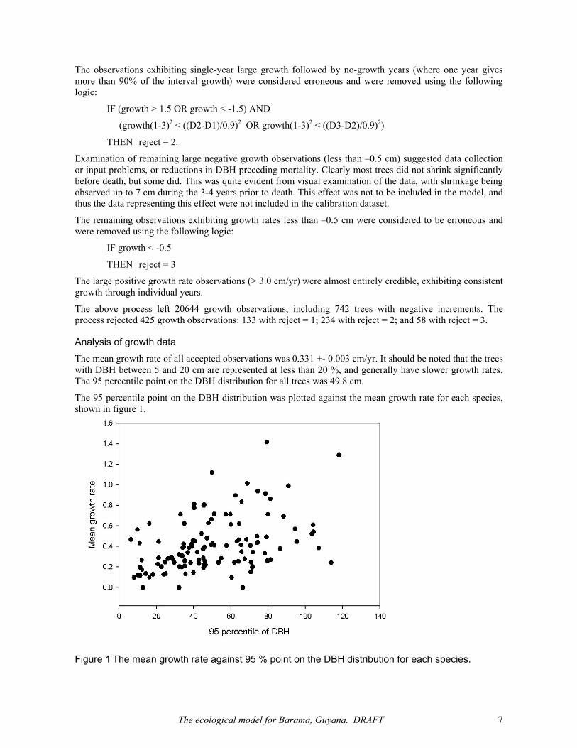
Analysis of growth data The mean growth rate of all accepted observations was 0.331 +- 0.003 cm/yr. It should be noted that the trees with DBH between 5 and 20 cm are represented at less than 20 %, and generally have slower growth rates. The 95 percentile point on the DBH distribution for all trees was 49.8 cm.

The 95 percentile point on the DBH distribution was plotted against the mean growth rate for each species, shown in figure 1.

Figure 1 The mean growth rate against 95 % point on the DBH distribution for each species.


The 95 percentile point on the DBH distribution was plotted against the mean growth rate for each species that had a minimum of 10 growth observations, as shown in figure 2.

Figure 2 The mean growth rate against 95 % point on the DBH distribution for each species that had more than 10 growth observations in the data.

Clearly there is a general rule that species with larger maximum size grow faster. There are some very fast growing species present in this area, especially when compared to the Tropenbos dataset. The dominant species, in terms of the number of trees, are shown in table 2.


Local name Number of trees mean growth rate (cm/yr) 95 percentile point DBH (cm)

Kakaralli, black 4731 0.26 46.0

Haiariballi 2258 0.41 51.2

Kauta 1947 0.22 46.4

Trysil 1352 0.39 37.6

Awasokule 1219 0.13 14.4

Kurokai 907 0.52 44.3

Baromalli 883 0.35 65.8

Waiki 678 0.66 49.6

Maho, black 544 0.12 11.4

Yarriyarri, white 330 0.12 10.2

Maho 294 0.41 57.6

Congo Pump 271 1.12 49.9

Kairiballi 271 0.19 45.3

Moraballi 238 0.39 45.9

Swizzle stick 235 0.28 28.7

Yarula 216 0.38 86.5

Yarriyarri, black 211 0.20 22.8

Wild cherry 206 0.13 24.1

Crabwood 205 0.47 68.4

Table 2 The dominant species, in terms of the number of trees, with their mean growth rate and 95 percentile point on the DBH distribution.

3.4 Taxa groups The taxa were recorded with local, vernacular names, and these have been maintained in this document. For reference, Appendix B gives the scientific names of the dominant taxa.

In order to group the taxa, it was necessary to assess the population density for each taxon recorded in the data set. Table 3 shows that only 29 taxa were represented by more than 100 trees. This number progressively increased as the minimum number of trees decreased.

Minimum number of trees Number of taxa Number of trees % of sample

100 29 19064 87

50 53 20717 95

20 82 21579 99

1 127 21812 100

Table 3 Minimum number of trees in a taxon for the Pibiri permanent sample plots.


In comparison with data from the plots at Pibiri, it is worth noting a few features:

• There are fewer taxa overall (139 compared to 181);

• There are more tree records (22,000 compared to 10,000);

• There are more taxa from which to form the initial species groups (53 compared to 38).

The process for grouping taxa involved three stages: (1) a clustering analysis to make the groups using the most populous taxa; (2) discriminant analysis to add the less populous taxa to the existing groups; and (3) a subjective stage where taxa with little or no data were assigned to the groups.

Clustering analysis of populous taxa For each taxa, a set of variables was produced:

• Average growth rate at low competition;

• Average growth rate at medium competition;

• Average growth rate at high competition;

• Average growth rate of new recruits (DBH of 5-10 cm);

• D95, the 95-percentile point in the DBH frequency distribution (as an index of mortality behaviour).

Low and high competition levels were specified using the diameter-independent competition index C (eqn. 6) The parameters b0, b1 and b2 were evaluated by regression, and their values given in table 4.

Parameter Value Uncertainty

b0 (cm) 174 ± 2

b1 (cm) -0.25 ± 0.05

b2 -3.3 ± 0.1

Table 4 The values of parameters in the model of diameter-independent competition index.

Values of C above 2.0 were classed as being high competition, and values below –2.0 were classed as being low competition, with medium competition being defined between these values (-2 < C ≤ 2). It should be noted that in development of the model using the Pibiri data, the limits were +1.0 and –1.0, which reflects the lower forest stocking, and consequent lower variation in competition, than observed from the Barama data.

The 29 data points arising from the taxa with more than 100 observations were insufficient to form groups as many groups would have contained just one species. The grouping process thus used taxa with at least 50 trees, giving 53 species (Table 3). Data were evaluated for these species, and normalised so that the range of each variable was from 0.0 to 1.0. A clustering procedure was then used to group the species according to the normalised variable values.

The clustering process requires the user to decide how many groups there should be in advance. After a trial and error process examining the resultant cluster contents from differing numbers of clusters, twelve clusters were used to define the initial grouping.

Despite the minimum number of observations used to select species for use in the clustering process, many species had characteristic variable values that were determined from only a small number of observations. In these instances, a single anomalous observation could significantly alter the characteristic variable value, causing the clustering procedure to produce anomalous results. In addition, the clustering procedure does not ascribe weights to the characteristics that are used to form the groups, although these may be desirable for increasing the relative importance of particular characteristics to the resulting groups. For these reasons, an exploratory data analysis was used to adjust the cluster composition to remove anomalous groups or taxa that had been mis-assigned to a group.


Starting with 12 clusters, an attempt was made to incorporate the low-occupancy groups into the existing well-defined groups, and several subjective adjustments were made. In all, the clustering of 9 taxa were adjusted out of the total clustering process of 53 taxa. The result was 8 groups as summarised in Table 5.

Group N Dominant Taxa ingrowth P95DBH G(low) G(med) G(high) Ntrees

1 9 Awasokule, Black Maho 50 10 5 5 5 3037

2 8 Black Kakaralli, Kauta 50 40 10 15 10 7569

3 10 Haiariballi, Trysil, Kurokai 40 30 20 30 15 5489

4 9 Baromalli, Maho 30 60 20 40 25 1923

5 6 Swizzle stick, unknown 30 20 15 20 10 784

6 5 Yarula, Bulletwood 40 90 20 30 10 476

7 5 Waiki, Warakaioro 30 40 50 70 10 1018

8 1 Congo Pump 0 50 70 100 70 421

Table 5 The dominant species for each cluster and their characterstics. N refers to the number of species per group after the clustering process.

Characteristics of the groups that are immediately obvious from the above table include:

• Group 8 (Congo pump) recruits in the lowest competition environment, and grows the fastest: a classic pioneer group;

• Group 6 (Yarula, Bulletwood) trees grow to the largest diameters;

• Group 1 (Awasokule, Black Maho) are the smallest and the slowest growing trees;

• Groups 2 and 3 contain the majority of the trees, and are not ecologically distinctive;

• Group 1 included the species Kurobete, which grows at less than 1 mm per year and 95 % of stems over 5 cm are found with a DBH less 8.1 cm.

The grouping was tested against alternative characteristics, and found to be robust.

The discriminant analysis: for less populous taxa Remaining ungrouped taxa with a minimum of 20 observations (29 taxa) were added to the existing groups using discriminant analysis. The data from the existing groups were used as training data to initialise this process. The characteristics used to define groups were the 95 percentile point on the cumulative DBH distribution and the mean growth rate.

Three taxa (Bloodwood, Arisauro and Maporokon) were not assigned to groups in the discriminant analysis. Bloodwood and Arisauro were assigned subjectively to the nearest group. Maporokon, with a mean growth rate of 1.4 ± 0.2 cm yr-1 (22 observations) and a 95 percentile point of DBH of 92 cm (19 observations), did not fit easily into any existing group. The obvious solution to this, to create a new group, was not satisfactory because there were only 19 growth measurements, and far fewer mortality and recruitment observations, from which to calibrate a model. Group 8 (Congo Pump) do not grow to as large a size as Maporokon, and group 6 (Bulletwood) grow much slower. In whichever group Maporokon is placed its characteristics would be lost, due to the relative numbers of trees. However, there was no option since there were not enough data to form a separate group. The size characteristic was given precedence and Maporokon was added to group 6.

Four other species were moved between groups subjectively following exploratory analysis of the discriminant analysis results.

Adding the remaining taxa to groups


The remaining 45 taxa, representing 233 tree records, were grouped using a second discriminant analysis. An additional 27 taxa were included in the species code list, but were not represented in the tree dataset. The lack of data for these taxa resulted in the 95 percentile point of DBH and mean growth rate being associated with large uncertainties. These data were used in the absence of alternative published sources of information.

The 95 percentile point of DBH and mean growth rate for these taxa were indicative either of their characteristics, or of the lack of data. In either case, it was appropriate for modelling purposes to use these variables to group the taxa. The rationale behind this was that taxa with almost no data were almost completely irrelevant, and others should have their data characteristics used as far as possible, especially in the absence of more subjective information. Thus the same discriminant analysis was performed on these data as on the species with between 20 and 50 trees.

14 taxa were not grouped by the second discriminant analysis due to not having any growth data. Kaditiri, Locust, Kumakaballi and Sawari were added to group 6, since large individuals of those species existed in the data and therefore demonstrated the species ability. The other 10 species were added to group 2, since it had approximately average values of 95 percentile point of DBH and mean growth rate.

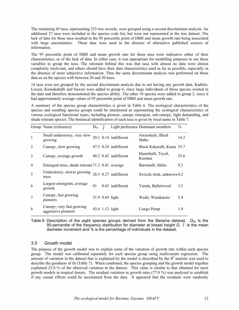
A summary of the species group characteristics is given in Table 6. The ecological characteristics of the species and resulting species groups could be interpreted as representing the ecological characteristics of various ecological functional types, including pioneer, canopy emergent, sub-canopy, light demanding, and shade tolerant species. The botanical identification of each taxa is given by local name in Table 7.

Group Name (reference) D95 I Light preference Dominant members %

1 Small understorey, very slow growing 20.1 0.14 indifferent Awasokule, Black

Maho 14.2

2 Canopy, slow growing 47.5 0.24 indifferent Black Kakaralli, Kauta 35.7

3 Canopy, average growth 48.2 0.42 indifferent Haiariballi, Trysil, Kurokai 25.6

4 Emergent trees, shade tolerant 71.3 0.41 average Baromalli, Maho 9.3

5 Understorey, slower growing trees 28.5 0.27 indifferent Swizzle stick, unknown 4.2

6 Largest emergents, average growth 91 0.43 indifferent Yarula, Bulletwood 3.5

7 Canopy, fast growing pioneers 51.9 0.69 light Waiki, Warakaioro 5.4

8 Canopy, very fast growing aggressive pioneers 43.6 1.12 light Congo Pump 1.9

Table 6 Description of the eight species groups derived from the Barama dataset. D95 is the 95-percentile of the frequency distribution for diameter at breast height D, I is the mean diameter increment and % is the percentage of individuals in the dataset.

3.5 Growth model The purpose of the growth model was to explain some of the variation of growth rate within each species group. The model was calibrated separately for each species group using multivariate regression. The amount of variation in the dataset that is explained by the model is described by the R2 statistic was used to describe the goodness of fit (Table 7). When combined, the species grouping and the growth model together explained 23.0 % of the observed variation in the dataset. This value is similar to that obtained for most growth models in tropical forests. The residual variation in growth rates (77.0 %) was analysed to establish if any casual effects could be ascertained from the data. It appeared that the residuals were randomly


distributed and it is assumed that this variation results from effects including measurement error, genetic effect and site specific effects and events such as pests, diseases and weather. It should be noted that a further, more in-depth study could investigate whether climbers or crown form affect growth rates. This was not attempted in the current study.

Group a0 a1 a2 a3 a4 R2 (%)

1 -1.4549 1.466 0.000 -0.0079 0.0603 9.4

2 0.0056 0.035 0.080 -0.0128 0.0038 4.9

3 0.0101 0.103 0.065 -0.0252 -0.2604 10.6

4 0.0006 0.014 0.021 -0.0305 0.2027 4.7

5 0.0134 0.116 0.129 -0.0210 -0.1684 7.5

6 0.0025 0.023 0.024 -0.0236 0.0854 8.6

7 0.0090 0.141 0.058 -0.0509 -0.2628 7.1

8 0.0103 0.145 0.072 -0.0363 0.2791 2.6

Table 7 Parameters for the Barama growth model (eqn. 1) and the associated goodness of fit R2 (%) within each species group.

3.6 Recruitment model The probability of ingrowth was estimated at the scale of individual 10x10m gridsquares as a function of competition index C. The competition index was calculated for a “virtual” tree with D of 5 cm at the centre of each gridsquare. This was used to create a frequency distribution of the competition index for all gridsquares. The frequency distribution was generated using seven bins for competition index

Data from the permanent sample plots were analysed for each species group to record the number of gridsquares in which ingrowth was observed and its associated competition index. If more than one individual of a species group was observed, the gridsquare was recorded once for each individual. The probability of ingrowth F was calculated for observed data was calculated:

GNNF F= (15)

where NF is the number of gridsquares with recruitment and NG is the total number of gridsquares within the stated competition index range. The probability of recruitment was modelled using equation 7 as a function of predicted growth rate I’ calculated for each species group within a specified competition index bin. These data were then used to calibrate equation 7 using regression.

The data points used for regression (one for each combination of species group and competition index bin) were weighted by the the number of grid-squares in each growth rate bin multiplied by five times the number of ingrowth observations for that bin total number of sub-plots in each growth rate bin. The calculation of R2 was suitably adjusted to include the weighting.

The resulting regressions produced value for R2 ranging from 48 to 98 %.

No data were available to estimate TI, the ingrowth time parameter. This was estimated for each species group from the mean observed diameter increment for trees in the 5-6 cm size class. The distribution of observed increments were not normally distributed and the value of the 75-percentile of I was used to calculate TI:

75I

5I

T = (16)


The estimate is subject to a significant uncertainty since it is not based on data. Alternative methods of calculation, such as the mode or geometric mean would be equally applicable.

Final recruitment parameter values are given in Table 8.

Group c1 c2 C3 c4 R2 TI

1 -10.220 -0.63 7.051 10.252 51.7 46

2 2.595 -0.69 -1.863 -2.548 75.4 37

3 0.001 -8.24 0.252 0.041 83.6 34

4 0.000 -7.71 0.021 0.006 94.7 24

5 -0.796 -0.34 0.361 0.798 48.0 27

6 0.000 -7.48 0.054 -0.001 61.8 27

7 0.000 -9.08 0.120 -0.004 90.5 14

8 0.000 -6.32 0.041 -0.027 98.2 5

Table 8 Parameter values for the recruitment model (eqn. 7)

3.7 Mortality model The mortality probability was modelled as a function of diameter. The calibration was achieved using the assumption that the diameter distribution for each species group in primary forest does not change with time. The potential problem with the approach is that clearly some of the forest represented by the data had been heavily logged (indicated by the large ingrowth of Congo Pump trees, relative to the pre-existing population). The history of individual plots was not reliably recorded with this dataset. A heavily logged forest may be expected to show a significantly different DBH distribution to that of natural forest.

If the mortality model were developed using the DBH distribution from logged over forest rather than unlogged natural forest, what would be the effect? The resulting mortality model would be such as to maintain the DBH distribution in its prior state; i.e., logged over. The whole forest model would not be expected to regenerate a natural forest. To ameliorate this effect, data were selected from plots that showed less than 5 % reduction in total basal area during the first measurement interval. As has already been noted, there was reason to believe that observations from the first survey were not as reliable as subsequent observations, but there was no choice, since this was the only available indicator of plot history.

Data were used from all plots that were not labelled as “abandoned”, did not decrease in basal area by more than 5 % over the first survey interval, and were not plot numbers: 6, 8, 10, 11, 28, 30, 31, 32, 33 or 42 (these were rejected due to data recording anomalies identified during exploratory analysis). The remaining 12 plots used in this analysis were: 1, 15, 17, 18, 21, 24, 26, 29, 36, 39, 49 and 50. DBH observations from survey 2 were used, since these were found to be more reliable than those from survey 1.

The DBH observations were grouped into DBH bins, whose width was dependent on species group: some species had DBH distributions from 5 cm to 120 cm, others from 5 cm to 30 cm. The bins needed to be of equal width, to start at 5 cm and to have a boundary at 20 cm, in order to use all the data and correctly handle the reduced sampling of smaller DBH trees. The optimal bin width was that producing 10 bins for each species group, but this didn’t necessarily form a boundary at 20 cm as required. The optimal bin width was thus given, for each species group, by:

optbinwidth = (maxdbh+1 – 5)/10 (17)

and the actual bin width to be used was:

binwidth = 15/ int( (15/optbinwidth)+0.5 ) (18)


The mean DBH for each bin was used as the x co-ordinate, rather than the mid-point of the bin, since the distribution was curved. The number of live tree observations for small trees was adjusted to compensate for the lack of sampling in these DBH regions. Most 1 ha plots included 0.2 ha of forest where all trees from 5-20 cm were measured. Exploratory analysis showed that plot 1 had only 0.12 ha, however, and plot 26 had only 0.16 ha. Thus the 12 plots used in this analysis had a total sample of 2.28 ha that included observations of small trees. The number of live trees in bins that had a mean DBH less than 20 was multiplied by 12/2.28 to compensate for lesser sampling (2.28 ha compared to 12 ha for the larger trees). Generally this did not lead to step-functions in the DBH frequency distribution, indicating that sampling of trees below 20 cm was sufficient for scaling up.

The shape of the size class distribution was modelled for each species group as a function of mean DBH D : )5(

2)5(

031 −−−− += DpDp

L epepN (19)

where NL is the number of live trees in a size class and p0, p1, p2 and p3 are constants evaluated by regression..

A typical DBH frequency distribution is classically referred to as an “inverse-J” distribution which can be modelled by a negative exponential functional. Several of the species groups in the Barama dataset exhibited more complex distributions (groups 3, 4, 5, 6 and 7), and a combination of two negative exponentials was required to model these groups.

The probability of mortality was calculated for each combination of species group and diameter size class. The assumption was made that the mortality probability is the same as the fractional decrease in numbers of live trees within a size-class, when that size-class experiences one year’s growth, required to maintain the diameter distribution. The growth equation (1) was applied to the mean DBH ( D ) using a value of zero for the competition index C to predict the mean diameter of the size class after one years’ growth ( 1' +tD ). The probability of mortality, M, was then calculated, for each species group and diameter size class, as:

DDDM t 1' +−

= (20)

The probability distribution of natural mortality with diameter for each species group was modelled using equation 8 and the values of parameters evaluated by regression. Parameter m0 represents the probability calculated for the smallest diameter class. Parameter D95 represents the 95-percentile point in the DBH distribution. Parameter m5 was evaluated by tuning the model to meet the requirement of dynamic equilibrium in unlogged primary forest. The parameters used in the mortality model are shown in Table 9.

Group Bin width m0 m1 m2 m3 m4 m5 D95 R2 (%)

1 3 1.6 -97.5 0.0103 -0.6562 99.1 0.03 20.1 100.0

2 7.5 1.0 0.7 0.0541 0.0409 0.4 0.05 47.5 100.0

3 7.5 2.0 4.8 0.0383 0.0707 -1.1 0.20 48.2 99.8

4 15 0.63 -0.58 0.1765 -0.0028 1.0 0.20 71.3 93.0

5 5 0.85 4.78 0.0649 0.2104 -0.7 0.03 28.5 100.0

6 15 0.75 2.0 0.0689 0.0021 0.5 0.10 91.0 99.6

7 7.5 8.0 106.71 0.0033 0.2918 -101.6 0.25 51.9 90.1

8 5 6.75 8.63 0.2528 0.0014 2.6 0.4 43.6 99.2

Table 9 Parameters for the mortality model, equation 8, with the bin-width of diameter used in calibration and the goodness of fit statistic, R2 .


Removing damaged trees The death of trees damaged by other trees dying and falling in the SYMFOR framework is simulated independently from natural mortality. The Barama data did not contain information that was useful in analysing the effects of damage. Some modelling of damage was required, however, and, lacking more relevant data, those from the Tropenbos dataset were used.

Small tree data generation Data representing small trees (5-20 cm) were generated for the model using equation 9. This equation was calibrated by generating a diameter frequency distribution for each species group for the sub-plots containing trees in the 5-20 cm size class. A frequency distribution of DBH was generated using data from 10 of the 15 plots. The other five plots were retained for validation of the procedure. The frequency distribution was generated using 3 cm size classes to generate 5 bins in the 5 to 20 cm range for each species group. The analysis utilised data from the 1993 survey as these data represented unlogged primary forest. The parameter g was determined by regression. The total number of trees per hectare of each species group (nt) in the size class of 5 to 20 cm was determined as the average from the 10 plots used in the size class distribution. The parameter values for each species group are shown in Table 10.

Group g nt

1 0.35 304

2 0.16 293

3 0.23 223

4 0.14 53

5 0.19 59

6 0.16 25

7 0.25 25

8 0.00 0

Table 10 Parameters used in the generation of small trees (5 ≤ D < 20 cm) using equation 9.

Species group 8 does not have any trees in the generated set because of its pioneer characteristics: if and when the canopy is opened significantly, this group would be expected to be recruited. The above parameter values were calibrated using data from unlogged forest, where there would be little canopy opening and thus little opportunity for pioneer species.

3.8 Evaluating and tuning the model The Barama model described above was implemented in SYMFOR framework. The model was tested using data from primary forest using the hypothesis that such forest should remain in dynamic equilibrium. This hypothesis was used as a basis to evaluate and tune the parameters of the model.

Initial evaluation The parameters that were varied as a result of this process were those considered to have the largest uncertainty resulting from the process of calibration:

• Mortality probability slope parameter for trees with large DBH values (m5);

• Mortality probability for small trees (m0);

• Mortality probability constant component (m4); and

• The overall recruitment probability (r1, r3 and r4: scaled together by the same amount).


Changes to these parameters were made incrementally over many repeated simulations. The parameters of the model demonstrated significant interactions often resulting from the underlying ecological nature of the model.

The performance of the model was evaluated using descriptive data output by the model at intervals during an extended simulation of 350 years. The basal area and number of stems within a species group were used to evaluate the model. It was expected that, whilst these values would vary with time in individual simulations, the mean of many simulations over time would remain unchanged.

Initial analysis of the model demonstrated that some of the parameters needed to be altered in order to achieve adequate performance. Selected model parameter values were tuned to improve performance in order to demonstrate a dynamic equilibrium in primary forest.


4 Discussion The characteristics of the Barama model are discussed in terms of the characteristics of the species groups derived from the data and a series of figures demonstrating the performance of the resulting model in primary forest and after simulated logging.

4.1 Simulations of primary (unlogged) and logged forest. The Barama model was tested in the SYMFOR framework. These applications are illustrated here.

The predicted growth rates for each species group are shown as Figure 3. Groups 1 and 5 are small, slow growing species. The highest growth rates were predicted for group 8 which is dominated by Congo Pump. The largest trees were from species group 6, dominated by Yarula and Bulletwood.

Figure 3 Predicted growth rates as a function of DBH. These rates were calculated for average competition (C = 0). The values are shown for the range from the minimum diameter of 5 cm up to the 99 percentile of the diameter frequency distribution for each species group.

The performance of the model was assessed by examining changes in the basal area and number of stems in each species group over time for unlogged primary forest. Figure 4 show one example simulation reporting the total basal area of the plot (all species groups,). The total basal area shows some interannual variability, but the trend is that total basal area remains relatively constant.

Ecological models interact with management models in the SYMFOR framework. The purpose of the framework is to provide a tool to support analysis of management and policy options for tropical forests. A simple logging treatment was simulated in the SYMFOR framework by removing the twenty largest trees in the one hectare plot. It should be noted that this level of extraction is many times more severe than current management practice in Guyana, and that the examples presented here are intended only to illustrate the performance of the model, and the interaction between the management and ecological models.


Figure 4 Variation in total basal area with time for 1 ha of unlogged primary forest. No management interventions wer simulated. This figure was taken directly from the time-series plotter in SYMFOR.

Figure 5 The sum of volume over all trees of each species group against time, showing forest development after logging. The forest from which the initialisation data were taken was unlogged, but logging was simulated (the largest 20 stems removed) in the first year of the run. 10 replicate runs were made, and the figure shows the mean results. A dynamic equilibrium appears to be established after approximately 150 years.


The management treatment was applied in this example to a one-hectare plot. The total volume (Figure 5) and number of stems (Figure 6) of each species group and balance between groups changed significantly following logging. The time required to reach a equilibrium between the groups is predicted to be around 150 years. This is similar to the comparable length of time for forests in Southeast Asia using similar analysis with the East Kalimantan model in the SYMFOR framework, and much faster than the comparable length of time for the model developed using the Tropenbos data. The reason for this latter difference is likely to be the much lower annual growth rates observed in central Guyana compared to NorthWest Guyana.

Figure 6 The number of trees of each species group against time, showing forest development after logging. The forest from which the initialisation data were taken was unlogged, but logging was simulated (the largest 20 stems removed) in the first year of the run. 10 replicate runs were made, and the figure shows the mean results.


5 Assumptions and limitations

5.1 Assumptions This section describes the assumptions required for the development and implementation of the Barama ecological model described in this document. Other models within the SYMFOR framework, including management models, that have their own associated assumptions that are not described here.

Data generation 1. The number of small trees in each species group with DBH in the range of 5 to 20 cm is the same in

every plot at the start of a simulation;

2. The small trees with DBH from 5 cm to 20 cm are established at random locations within the plot at the start of each simulation;

Growth model 3. Trees grow deterministically as a function of their species group, diameter and competition

environment;

4. Trees cannot decrease in stem diameter;

5. Competition is only caused by larger neighbouring trees within a 30 m radius of the tree;

6. No competition is experienced by a tree from neighbouring trees that are more than 30 m away;

7. Competition does not increase as a function of distance to a neighbouring tree for distances less than 3 m;

8. Small trees with diameters of less than 20 cm only produce competition for other trees in the same 10x10m grid square. This competition is density dependant and not related to distance;

Recruitment model 9. The probability of recruitment is a function of predicted growth rate;

10. The probability of recruitment may be non-zero even when the predicted growth rate is zero;

11. Seedlings and saplings with a diameter between 0 cm and 5 cm grow with the same diameter increment as trees with a DBH between 5 cm and 6 cm;

12. A constant supply of seedlings exists for all species groups, except shortly after an area has been cleared (as part of a management process);

Mortality model 13. Mortality is stochastic (a random event), and is described as a function of species group and

diameter;

14. The probability of a tree falling immediately after natural death is 50 %. All other trees are assumed to rot whilst standing and cause no additional damage to the residual stand;

15. The area under which damage may occur resulting from a falling tree is described by a kite-shape;

16. There are no catastrophic mortality events (drought, flood, hurricane, etc) described in the model, and the effects of such processes are captured in the mean rates of mortality;

Other assumptions 17. The behaviour of all trees within a species group is specified in the same way;

18. Trees at the edge of the simulated plot interact with trees on the other side of the plot, through plot-wrapping;


19. All sites are equivalent, in terms of their ability to support tree species compositions and diameter distributions;

20. All sites are equivalent, in terms of their suitability and access for logging and other management activities;

21. Non-modelled phenomena (such as climate, the presence of climbers, pests, disease, watercourses, slope, soil-types, etc.) are constant over time and are the same as for the data used for calibration;

22. The calculations of stem basal area and volume assume that all trees are circular in cross-section;

23. The calculation of stem volume assumes that all trees have the same taper and volume to basal area ratios;

In a given simulated year, the forest processes are simulated in the following order: management, growth, mortality, recruitment.

5.2 Limitations The model should only be applied to areas of forest with similar soils, species composition and tree density as the plots used to calibrate the Barama model. The rates of growth, recruitment and mortality should be similar to those observed in the Barama sample plots. In practice, this means primary or managed natural forests in the Guyana shield in north-eastern South America on the same soils as Barama.

The suitability of the model should be evaluated before it applied to new areas or forest types. Data from the new area should be compared with those used for calibration of the Barama model. The nature of the comparison will depend on whether repeated diameter measurements are available to estimate growth rates.

In all cases the user should compare:

• Stand basal area and volume

• Stand density

• Species composition by individual species and ecological species groups. This comparison should consider the number of stems in each taxa and their total basal area.

If repeated measurements are available from permanent sample plots, these should be used to calculate mean diameter increments for each species groups. These should be compared with the values reported in Table 7.

The method of comparison will need to be subjective and result in an assessment of how similar the new area is to the Barama plots used for calibration.. In the absence of sufficient information for the above analysis, a more simple comparison should be made with whatever data is available, and suitable provisos appended to the description of any simulation results.


6 Conclusions The Barama ecological model has been developed, calibrated and implemented within the SYMFOR framework. This implementation was then tested and tuned against the criteria that the structure of an unlogged primary forest should not change significantly with time.

The ecological species groupings and initial simulations with the model describe ecologically relevant characteristics and processes in the forest. The results indicate that this forest is characterised by relatively slow growing species and that this forest type requires very long periods to recover after major disturbance.

The model is suitable for use with data from Barama, North West Guyana, or other areas of similar forest. Subsequent distributions of SYMFOR will include this ecological model, which is called “Guyana-Barama”.

Applications of the model will be published separately.


7 Acknowledgement The authors would like to acknowledge the staff of Barama Company Limited, Guyana Forestry Commission and the DFID GFC-support project for the provision of the data necessary for this work, assistance in data processing and their comments on the model.


8 References Alder, D., 2000. Development of growth models for applications in Guyana. Technical report for the Guyana

Forestry Commission Support Project, 47 pgs.

Alder, D., 2001. Pers. Comm. Excerpt from: Unknown author (unknown year). ECTF manual of research methods. ECTF consultancy report for the Barama Company Limited, Georgetown, Guyana.

Bird, N., 2001. On: The low levels of natural damage observed in forests in Guyana. Pers. Comm.

Phillips, P.D., Brash, T.E., Yasman, I., Subagyo, P., van Gardingen, P.R., 2002a. An individual-based spatially explicit tree growth model for forests in East Kalimantan (Indonesian Borneo). Ecol. Model. (in press).

Phillips, P.D., van der Hout, P., Arets, E.J.M.M., Zagt, R.J., van Gardingen, P.R., 2002b. Modelling the natural forest processes using data from the Tropenbos plots at Pibiri, Guyana. SYMFOR technical note series no. 9, The University of Edinburgh, Edinburgh, 25pp. http://www.symfor.org/technical/index.html

Phillips, P.D. and van Gardingen, P.R., 2001. The SYMFOR framework for individual-based spatial ecological and silvicultural forest models. SYMFOR Technical Notes Series No. 8, The University of Edinburgh. http://www.symfor.org/technical/framework.pdf

Phillips, P.D., 2001. Development of Modelling Objectives, Guyana: Back to Office Report. The University of Edinburgh, Edinburgh, 30 pgs. http://www.symfor.org/btor/Guyana_jun01.pdf

Phillips, P.D., van der Hout, P., Zagt, R.J., van Gardingen, P.R., 2002. An ecological model for the management of natural forests derived from the Tropenbos permanent sample plots at Pibiri, Guyana. SYMFOR Technical Notes Series No. 9, The University of Edinburgh. http://www.symfor.org/technical/pibiri.pdf

ter Steege, H., 2000. Plant diversity in Guyana: with recommendations for a protected areas strategy. Tropenbos Series 18, Tropenbos Foundation, Wageningen, Netherlands.

van Gardingen, P.R., 2001a. Project Memorandum (Exit Strategy) FRP project R6915. The University of Edinburgh, Edinburgh, 89 pgs.

van Gardingen, P.R., 2001b. Partnership Building FRP Projects R6915, R7278, ZF0151: Back to Office Report. The University of Edinburgh. 90 pgs. http://www.symfor.org/btor/partnership_mar01.pdf


9 Appendix A – The model parameters Table 11 shows the model parameters as described in the text, a summary of their usage, and the corresponding variable name in the SYMFOR computer program code.

Parameter Name in SYMFOR Usage

a0 – a4 p0 – p4 (species group) Growth model coefficients

b0 – b2 dicomp1, dicomp2, dicomp3 Diameter-independent competition model coefficients

r1 – r4 i1 – i4 (species group) Recruitment model coefficients

m0 – m5 b0 – b5 (species group) Mortality model coefficients

D95 p95 (species group) An effective maximum tree DBH

7.5 cm mbinwidth The width of the smallest DBH bin for mortality modelling

TI ingrowthtime (species group) The minimum time for a seed to reach a DBH of 5 cm

G gendist (species group) Coefficient in the model of DBH distribution for small trees

nt ntreesph (species group) The number of trees per ha to be created at model initialisation

5 cm dbhmin The minimum DBH of trees to be created at model initialisation

20 cm dbhfill The maximum DBH of trees to be created at model initialisation

fC a (species group) The fraction of tree height at which the crown begins

Hm maxheight (species group) The maximum height of a tree of any diameter

s startslope (species group) A coefficient in the equation relating height to DBH

fV formheight (species group) The ratio of basal area to modelled timber volume

Table 11 A summary of the model parameters.


10 Appendix B – scientific names of dominant taxa Table 12 shows the scientific name for each of the dominant taxa, labelled by vernacular name, with their species group.

Vernacular Group Family Genus Species

Awasokule 1 Guttiferae Tovomita

Black maho 1 Sterculiaceae Sterculia exsucca

Black kakaralli 2 Lecythidaceae Eschweilera sagotiana

Kauta 2 Chrysobalanaceae Licania guianensis

Haiariballi 3 Papilionaceae Alexa

Trysil 3 Mimosaceae Pentaclethra odorata

Kurokai 3 Burseraceae Protium dacandrum

Baromalli 4 Bombaceae Catostemma

Maho 4 Sterculiaceae Sterculia pruriens

Swizzle stick 5 Euphorbiaceae Mabea

Unknown 5

Bulletwood 6 Sapotaceae Manilkara bidentata

Yarula 6 Apocynaceae Aspidosperma

Waiki 7 Mimosaceae Inga rubiginosa

Warakaioro 7 Flacourtaceae Laetia procera

Congo pump 8 Moraceae Cecropia angulata

Table 12 The scientific names of the dominant species in each group, corresponding to the local (vernacular) names used elsewhere.

an ecological model for the management of natural … ecological model for barama, guyana. draft ii...

Documents