I. l.cport No.

TX-91/1221-lF

An Assessment of Transportation Infrastructure Needs

7. AWaor(a)

William F. McFarland, Margaret K. Chui and Jeffery L Memmott

9. ~ Orplllilolica ,._ - ~

Texas Transportation Institute The Texas A&M University System College Station, Texas 77843-3135

Texas Department of Transportation Transportation Planning Division P.O. Box 5051, Austin, Texas 78763

U. SllFJ' ''Y N-

TECHNICAL REPORT ST AND ARD TITI..E PAGE

~ . ...-Due f ebruan:

121, 1991

•ulv 1991 Revised

l ........... ~a,._No.

Research Report 1221-lF 10

• w~dy No. 2-1-88/90..1221

II, C- ,.. 0.. No.

Final - Jan. 88 to Aug. 90

Researcb Study Title: An Assessment of Transportation Infrastructure Needs

16. Aholnld Four reports recently published by the Federal Highway AdlilllllStration (.t WA), tne American Association of Highway and Transportation Officials (AASHTO), the National Council on Public Works Improvement, and the Congressional Budget Office ( CBO) present information that is important in evaluating highway needs in the United States. The objective of this study is to provide a comparison and critique of these four reports. Special emphasis is placed on evaluating the rate-of-return analysis for highway investment in the Congressional Budget Office's report entitled New Directions for the Nation's Public Works, which was published in September, 1988.

Even using the CBO procedure and the CBO's assumed (implicit) useful lives, it can be concluded that about $25 billion dollars of investment in 1985 (and increasing over time at the same rate as traffic growth) is economically justified for highway investment on existing locations, as compared to an actual expenditure of about $13 billion in 1985. However, the CBO uses the assumption that investments made at the end of the analysis period give only 10 years of benefits. Using a more realistic useful life for highway investments would justify a somewhat higher investment level, probably considerably more than· double current capital spending.

The corrected results using CBO's own analysis procedure support the National Council on Public Works Improvement's recommendation that capital spending for highways should be _ ... 1 ___ ... ..J-,.t..1- ..J

17. Key Words

Infrastructure Investment, Investment analysis, Highway needs, Benefit·cost, Rates of return

11• DIMriloutD ~o restrictions. This document is

available to the public through the National Technical Information Service, 5285 Port Royal Road, Springfield, VA 22161

19. Securk)< Cllooit. (ol thio -') 31. Socuriry Cloooit. (al thio .....> 21. No.of Pa..,.

Unclassified Unclassified 86

J:'nnTi noT J:' t 7M '7 111:..AO\

AN ASSESSMENT OF

TRANSPORTATION INFRASTRUCfURE NEEDS

Report Prepared for

Texas Department of Transportation

by

William F. McFarland

Margaret K.. Chui

and

Jeffery L Memmott

Texas Transportation Institute College Station, Texas 77843

February 1991 July 1991/Revised

METRIC (SI*) CONVERSION FACTORS

APPROXIMATE CONVERSIONS TO SI UNITS APPROXIMATE CONVERSIONS TO SI UNITS Symbol wtMlft You Know Multiply By To Find Symbol Symbol W...n You Know Multiply By To Find Syrftbol

LENGTH LENGTH .. -In centimetres - mm millimetres 0.039 Inches In

Inches 2.54 cm - m metres 3.28 feet ft ft feet 0.3048 metres m

metres 1.09 yards yd yd yards 0.914

- m metru m km kilometres 0.621 miles ml

ml miles 1.81 kllometrea km --- AREA --AREA - mm• millimetres squared 0.0016 In• - square Inches

ln1 square lnchee MS.2 centimetres squared cm• - mt metres squared 10.76' square feet ft1

ft• square feet 0.0929 metres squared mt - km1 kilometres squared 0.39 square miles mil -yd• square yards 0.836 metres squared m' .. ha hectores (10 000 m') 2.53 acres ac -m11 square mlles 2.59 kilometres squared km1 -ac acres 0.395 hectares ha MASS (weight) --

i::: - g grams 0.0353 ounces oz

MASS (weight) - kg kilograms 2.205 pounds lb

- Mg megagrams (1 000 kg) 1.103 short tons T O.l ounces 28.35 -grams g lb pounds 0.454 kilograms kg .. T short tons (2000 lb) 0.907 megagrams Mg VOLUME

ml mlllllitres 0.034 fluld ounces fl oz L litres 0.264 gallons gal ...

VOLUME m• metres cubed 35.315 cubic feet ft1 - m• metres cubed 1.308 cubic yards yd• fl oz fluld ounces 29.57 millllltres ml - ...

~

gal gallons 3.785 litres L -tt• cubic feet 0.0328 metres cubed m•

.. TEMPERATURE (exact) - -yd• cubic yards 0.0785 metres cubed m• -- = °C Celsius 915 (then Fahrenheit Of

NOTE: Volumes greater then 1000 L shall be shown In m•. - ... temperature add 32) temperature = - = Of - .. Of 32 98.1 212 - - -f' ' '?'' ~4;0 I' 't?0 • b/~· I ,t!"'. • ,2tl°J TEMPERATURE (exact) ; -i ~ = -.&0 f -io I 0 io I I 80 r Bo I 100 .. - ~ ~ ~ •F Fahrenheit 519 (after Celslus °C temperature subtracting 32) temperature These factors conform to the requirement of FHWA Order 5190.1A.

• SI Is the symbol for the lntematlonal System of Measurements

PREFACE

The authors would like to thank Mr. Tom Griebel, Director of the Planning and Policy Division of the Texas Department of Transportation for serving as technical advisor on this study. Mr. Harry Caldwell and Ms. Regina McElroy of the Federal Highway Administration, U.S. Department of Transportation, provided us with the United States data set used in the analysis of rates of return reported in Chapter m of the report. They also provided information on the assumptions and methodology used in the original FHW A analysis that was later used in the Congressional Budget Office study that is discussed in this report. Special thanks go to Dennis Christiansen, Tim Lomax, Mark Goode, and Dock Burke of the Texas Transportation Institute staff for their assistance with this research.

DISCLAIMER STATEMENT

The contents of this report reflect the views of the authors and do not necessarily reflect the official views or policies of the Texas State Department of Highways and Public Transportation. This report does not constitute a standard, a specification, or a regulation.

iii

EXECUTIVE SUMMARY

The objective of this study is to provide a comparison and critique of four recently­published reports that present evaluations of highway needs in the United States:

1. American Association of State Highway and Transportation Officials, Keepin& A.merica Movinia The Bottom Line: A Summary of Surface Trans.portation Investment Requirements. 1988-2020. Washington, D.C., September 1988.

2. Federal Highway Administration, The Future National Hi"hway Pro&ram: 1991 and Beyond. Wor.lcini Paper No. 13. Hi&hway Perfonnance and Investment Analysis, Washington, D.C., December 1987.

3. National Council on Public Works Improvement, Fra~le Foundations: A Report on America's Public Works, Final Report to the President and Congress, U.S. Government Printing Office, February 1988.

4. Congressional Budget Office, New Directions for the Nation's Public Works, U.S. Government Printing Office, September 1988.

For evaluating general transportation needs, AASHTO's Bottom Line is the most comprehensive report of the four in that it provides detailed estimates of needs for highway and road expenditures and for transit. FHWA's Workin& Paper 13 is important because it provides detailed benefit-cost ratios for highway expenditures and also because it provides background for better understanding the CBO report. The National Council on Public Works Improvement is a very important general report that gives recommendations for several types of infrastructure investment. The report basically recommends a doubling of infrastructure investment on the basis that the infrastructure is deteriorating in the U.S. and is vital for future economic growth. The CBO report follows the National Council report in evaluating needs for investment in several types of infrastructure and includes chapters on highways, mass transit, aviation, water transportation, and wastewater treatment.

Most previous estimates of highway and bridge needs have used engineering standards. These estimates typically define geometric and structural standards, and determine the amount of investment that will be needed over some period of time (such as 20 years) to bring highways and bridges up to the desired standard and to keep them at this standard throughout the 20 years. This type of analysis is the basis for the needs analysis of the Highway Performance Monitoring System (HPMS) which is used by the Federal Highway Administration to develop needs estimates. FHW A's needs estimates are reported to the U. S. Congress at two-year intervals. The HPMS analytical procedure includes detailed procedures for determining the types of investment needed on existing highways in the United States to maintain stated levels of service. HPMS also includes procedures for estimating highway user costs at different levels of service, corresponding to different levels of highway investment

iv

In addition to the engineering standards method, three other basic methods that have been used in recent studies to estimate highway investment needs include: (1) use ofbenefit­cost analysis to determine the level of highway investment that is economically justified, (2) use of rate-of-return analysis to determine the level of highway investment that is economically justified, and (3) estimation of the amount of investment in highways needed to sustain future economic growth.

One of these four methods of determining highway needs is used in each of the four studies reviewed in this report. AASHTO's Bottom Line report mainly uses the method of determining the level of investment needed to maintain different levels of engineering standards, even though the report does present some information on user costs and benefits. FHW A's :Workin& Paper 13 uses benefit-cost analysis to evaluate different investment scenarios. The CBO's New Directions report evaluates selected investment scenarios using the internal rate of return as an indicator of economic desirability. The National Council of Public Works Improvement's Fra~le Foundations report uses economic growth criteria as the principal reason for recommending an increase in investment in highways and other infrastructure.

Three of the above studies use HPMS output as the principal basis for evaluating highway investment needs. The AASHTO study uses the HPMS output for several scenarios directly. The FHWA and CBO reports use HPMS output as the basis for economic calculations, benefit-cost analysis in FHWA's Workini Paper 13 and rate-of-return analysis in the CBO report.

The AASHTO Bottom Line report projects surface transportation requirements for the years 1988 through 2020. The report uses the HPMS national database as the basis for making highway estimates and uses the national bridge inventory as the basis for making estimates of bridge investment needs. Highway maintenance and operation costs are estimated by adjusting current levels of these expenditures.

In general, the AASHTO report shows that there is a large backlog of highways and bridges that need capital improvement; base needs are growing; and there will be new requirements for future capacity, on existing and new locations. At current spending levels, highway performance will decline and the needs backlog will grow. Highway performance is measured by a composite index that considers pavement condition, motorist safety, and service, as measured by vehicle speeds and congestion. AASHTO also shows that vehicle operating costs will increase if increased investment is not made in highways.

The goal of the extensive study made by the National Council on Public Works Improvement (the "Council") was to determine the level of investment needed in infrastructure investment in the United States. The Council uses two principal criteria, in addition to previous needs studies such as those cited above, for evaluating the need for future infrastructure investment. The first of these is future industrial demand based on infrastructure use per dollar of output. The second measure is capital outlays for

v

infrastructure as a percent of GNP and as a percent of private investment.

The Council presents data showing that the investment in public works in the United States has declined as a percent of Gross National Product (GNP); the decline in capital expenditures for highways, streets, roads, and bridges as a percent of GNP has been especially large. The Council's major recommendation for future investment in public works is:

... the Council recommends a national commitment, shared by all levels of government, the private sector, and the public, to vastly improve America's infrastructure. Such a commitment could require an increase of up to 100 percent in the amount of capital the nation invests each year in new and existing public works. In 1985, this amount was approximately $45 billion.

The main objective of the CBO study was to evaluate the National Council's report and needs estimates. The main basis for this critique is the CBO's use of FHW A's HPMS data to estimate the rate of return on future highway investment in the United States. The CBO report is somewhat like the FHW A's Working Paper 13 in that each presents an economic analysis of investment scenarios, but the CBO puts the analysis in terms of rates of return instead of benefit-cost ratios.

The principal highway analysis of the CBO report is based on an analysis of what the CBO refers to as "maintenance" strategies. This could be misleading because these strategies include all types of HPMS model expenditures, most of which are capital investments that have relatively long service lives. These capital investments include lane widening, adding lanes, major reconstruction, and pavement overlays. The main thrust of the highway investment section of the CBO report is to estimate rates of return for various levels and types of investment in highway facilities. The source of information for these calculations is the analysis package developed by the Federal Highway Administration, called the Highway Performance Monitoring System.

One of the major objectives of the present TI1 study is to evaluate the rates of return developed by the CBO from the FHW A data. The actual computer runs used by the CBO were made by FHW A and provided to CBO; but the rates of return were developed by the CBO from the FHW A data. The national HPMS data set used for the CBO report was obtained and the TI1 copy of the HPMS analysis package was used to duplicate as nearly as possible the runs made by FHW A and used by CBO in their report. Additional runs were made using different investment levels. The rate of return calculations on those investment levels were estimated using the same procedure used by CBO. The evaluation allows for a comprehensive critique of the methodology and accuracy of the highway investment calculations in the CBO report. This also gives a much clearer picture of the validity of the conclusions reached in the CBO report.

Three major technical criticisms are made of the CBO report. ::E.im, the report

vi

(implicitly) uses very short useful lives for major highway improvements; benefits are considered for only 10 years for major investments made at the end of the investment period (year 2000) even though these types of facilities historically have had useful lives of greater than 40 years, as shown in the HPMS documentation reports. This use of shorter lives has a major impact on rates of return, and probably is the main reason that the CBO analysis shows small or even negative returns for some investment levels. Second, the CBO only uses the HPMS estimates of user cost savings in the year 2000 to estimate highway benefits, even though HPMS output provides estimates for intermediate years. The end-of-period estimates should be used since these are technically superior estimates than the CBO estimates. They use the actual HPMS intermediate output as well as the end-of-period output. This report shows how much this affects the CBO calculations. Ihi.r.Q, in its rate-of­return analysis, the CBO fails to calculate rates of return for a wide enough range of investment levels and this leads to erroneous interpretation of needed highway investments.

The Congressional Budget Office is to be commended for its attempt to develop rates of return for highway investments. This analysis, together with that performed by FHWA in WorkinK Paper 13, promises to give a better indication of the economically justified level of expenditure on highways. In this respect, the analysis technique afforded by the HPMS data and analytical programs provides a tremendous advancement in the state of the art for evaluating needs for this important public works investment. This is undoubtedly one of the most comprehensive and accurate procedures available for making this type of analysis for any type of public work. Nevertheless, the CBO study does not include estimates of rates of return for a wide enough range of investment levels. This study extends the CBO analysis by calculating rates of return for a wider range of investment levels. This analysis of a full range of investment levels considerably changes the conclusions reached from this type of analysis, indicating that a higher level of highway spending is desirable than that implied by the CBO report.

Even using the CBO procedure and the CBO's assumed (implicit) useful lives, it can be concluded that about $25 billion dollars of investment in 1985 (and increasing over time at the same rate as traffic growth) is economically justified. However, the unrealistic assumption in the CBO report that the last investments give only 10 years of benefits should be taken into consideration; using a more realistic useful life for highway investments would justify a somewhat higher investment level, probably considerably more than double current capital spending.

The extended results developed in this study using the CBO's analysis procedure support the National Council on Public Works Improvement's recommendation that capital spending for highways should be at least doubled.

vii

TABLE OF CONTENTS

Page METRIC CONVERSION FACTORS . . . . . . . . . . . . . . . . . . . . . . . . . . . . . . . . . . . ii PREF ACE . . . . . . • . . . . . • . • . . . . . . . . . . . . . . . . . . . • . . . . . . . . . . . . . . . . . . . . iii DISCLAI?dERSTATEMENT ...........•.•.....•.•..•.......•........ iii E.XECUTI'VE. SUMMARY • . . . • . . . . . . . . . . . . . • . . . . . . • . . . . . . . . . . . . . . . . iv T.ABLE OF CONIE~ . . . . . . . . . . . . . . . . . . . . . . . . . . . . . . . . . . . . . . . . . . . viii UST 0 F TABLES . . . . • . . . . . . . . . . . . . . . . . . . . . . . . . . . . . . . . . . . . . . . . . . . . . . ix UST OF FIGURES . . . . . . . . . . . . . . . .. . . . . . . . . . . . . . . . . . . . . . . . . . . . . . . . . xi

I. IN'1R.ODUCTION . . . . . . . . . . • . . . . . . . . . . . . • . . . . . . . . . . . . . . . . . . . . . . . . 1

Background . . . . . . . . . . . . . . . . . . . . . . . . . . . . . . . . . . . . . . . . . . . . . . . . . . 1 Purpose and Contents of Report . . . . . . . . . . . . . . . . . . . . . . . . . . . . . . . . . . 1

II. REVIEW AND CRIDQUE OF FOUR REPORTS . . . . . . . . . . . . . . . . . . . . . . 3

The HPMS Analytical Process . . . . . . . . . . . . . . . . . . . . . . . . . . . . . . . . . . . . 3 AASHfO's Bottom Line . . . . . . . . . . . . . . . . . . . . . . . . . . . . . . . . . . . . . . . . 6 FHWA's Workini Paper 13 . . . . . . . . . . . . . . . . . . . . . . . . . . . . . . . . . . . . . 17 National Council on Public Works Improvement's Fragile Foundations Report . . . . . . . . . . . . . . . . . . . . . . . . . . . . . . . . . . . . . 19 CBO New Directions in Public Works . . . . . . . . . . . . . . . . . . . . . . . . . . . . . 22 Concluding Comments on the Four Reports . . . . . . . . . . . . . . . . . . . . . . . . . 29

III. EVALUATION AND CRIDQUE OF CBO ANALYSIS USING U.S. DATA . 33

Data V aria ti on . . . . . . . . . . . . . . . . . . . . . . . . . . . . . . . . . . . . . . . . . . . . . . 33 User Costs Calculation . . . . . . . . . . . . . . . . . . . . . . . . . . . . . . . . . . . . . . . . . 34 Traffic Growth Rates . . . . . . . . . . . . . . . . . . . . . . . . . . . . . . . . . . . . . . . . . . 36 Funding I..evels • . . . . . . . . . . . . . . . . . . . . . . . . . . . . . . . . . . . • . . . . . . . . . 36 User Costs and Savings . . . . . . . . . . . . . . . . . . . . . . . . . . . . . . . . . . . . . . . . 36 Internal Rates of Return . . . . . . . . . . . . . . . . . . . . . . . . . . . . . . . . . . . . . . . 44 Summary and Concluding Comments . . . . . . . . . . . . . . . . . . . . . . . . . . . . . . 52

N. OTIIER ASPECT'S OF TIIE CBO STUDY . . . . . • . . . . . . . . . . . . . . . . . . . . 53

V. INVESTMENT ANALYSIS FOR TEXAS . . . . . . . . . . . . . . . . . . . . . . . . . . • . 56

Traffic Growth Rates and Budget Levels . . . . . . . . . . . . . . . • . • . . • . . . . . . 56 Incremental Internal Rate of Return . . . . . . . . . . . . . . . . . . • . • . . . . . . . . . 56

REFERENCES . • . . . . . . . . . . . . . . . . . . . . . . . . . . . . . . . . . . . . . . . . . . . . . . . . . 71

viii

LIST OF TABLES

Page Table 1. 1985 Highway and Road Related Spending in the United States, 1985

Billions of Dollars . . . . . . . . . . . . . . . . . . . . . . . . . . . . . . . . . . . . . . . . 9 Table 2. Annual Highway Investment Needs by Scenario as Estimated in

AASHTO's Bottom Line Report, for the Time Period 1988-2020, Billions of Dollars . . . . . . . . . . . . . . . . . . . . . . . . . . . . . . . . . . . . . . . 11

Table 3. Change in Composite Index in Percent, Weighted by Daily Vehicle Miles Traveled, for Each Scenario, for the Time Period 1988-2020 . . . 12

Table 4. Requirements for New Highways in Urbanized Areas of the United States, in Lane Miles, 1986-2005 . . . . . . . . . . . . . . . . . . . . . . . . . . . . 13

Table 5. AASHTO's Estimate of Annual Highway, Road, and Bridge Expenditure Requirements, 1988-2020, in Billions of Dollars . . . . . . . 15

Table 6. AASHTO's Estimate of Total Annual Surface Expenditure Requirements, 1988-2020, in Billions of Dollars . . . . . . . . . . . . . . . . . 16

Table 7. Incremental Benefit-cost Ratios for Selected Investment Scenarios, from FHWA's Workin~ Paper 13 . . . . . . . . . . . . . . . . . . . . . . . . . . . . 20

Table 8. Three National Needs Studies: Comparison of Annual Capital Investment Requirements, in Billions of 1982 Dollars . . . . . . . . . . . . . 23

Table 9. Prospective Total Returns on Investment for Five Highway Maintenance Strategies, Under Low and High Traffic Growth, Using 1985 Prices . . . . . . . . . . . . . . . . . . . . . . . . . . . . . . . . . . . . . . . 26

Table 10. Prospective Incremental Returns on Investment for Five Highway Maintenance Strategies, Under Low and High Traffic Growth, Using 1985 Prices . . . . . . . . . . . . . . . . . . . . . . . . . . . . . . . . . 27

Table 11. United States Investment Costs of Seven Funding Strategies, at Low and High Traffic Growth Rates, 1985-2000 . . . . . . . . . . . . . . . . . . . . . 37

Table 12a. United States High Growth Funding Distribution, by Period and by Functional Class, 1985-2000 . . . . . . . . . . . . . . . . . . . . . . . . . . . . . . . . 38

Table 12b. United States Low Growth Funding Distribution, by Period and by Functional Class, 1985-2000 . . . . . . . . . . . . . . . . . . . . . . . . . . . . . . . . 41

Table 13. United States Daily-Vehicle-Mile Traveled, in Million . . . . . . . . . . . . 45 Table 14. United States User Savings of Seven Funding Strategies,

at High and Low Growth Rates for 1990, 1995 and 2000 • . . . . . . . . . 46 Table 15. United States Incremental Investment Costs and Incremental User

Savings of Seven Funding Strategies, at High and Low Growth Rates for 1990, 1995, and 2000 . . . . . . . . . . . . . . . . . . . . . . . . . . . . . . . . . . 48

Table 16. Internal Rates of Return (IRR) on United States Investments and Incremental IRR Using Two Methods . . . . . • . . . . . . . . . . . . . . . . . . 49

Table 17. Texas Investment Costs of Six Funding Strategies, at High and Low Growth Rates, 1985-2000 . . . . . . . . . . . . . . . . . . . . . . . . . . . . . . . . . . 57

ix

Table 18a.

Table 18b.

Table 19. Table 20.

Table 21.

Table 22.

LIST OF TABLES (Continued)

Page Texas High Growth Funding Distribution, by Period and by Functional Oass, 1985-2000 . • . . . . • . . . • . . . • . • . . • . . . . . . . . . 58 Texas Low Growth Funding Distribution, by Period and by Functional Oass, 1985-2000 • . . . . . . . . . . . . . . . . . . . . . . . . . . . . 61 Texas Daily-Vehicle-Mile Traveled, in Million . . . . . . . . . . . . . . . . . . 64 Texas User Savings of Six Funding Strategies, at High and Low Growth Rates for 1990, 1995, and 2000 . . . . . . . . . . . . . . . . 65 Texas Incremental Investment Costs and Incremental User Savings of Six Funding Strategies, at High and Low Growth Rates for 1990, 1995, and 2000 . . . . . . . . . . . . . . . . . . . . . . . . . . . . . 66 Internal Rates of Return (IRR) on Texas Investments and Incremental IRR Using Two Methods . . . . . . . . . . . . . . . . . . . . . . . . . . . . . . . . . . 67

x

Figure 1. Figure 2.

LIST OF FIGURES

Page Typical HPMS Analysis Output . . . . . . . . . . . . . . . . . . . . . . . . . . . . . . 7 FHWA's HPMS Benefit-Cost Procedure Used in Working Paper 13 • . . . . . • . . . . . . . • . . . . . . . . . . . . . • • . . • . • . . . • . . . . . . . 18

Figure 3. Total Public Expenditures for Highways, Streets, Roads, and Bridges in the United States [3, Exhibit A-2, p. 132] . • . . . . . . . . . . . . 24

Figure 4. Plot of CBO's Incremental Internal Rates of Return for Five Funding Strategies, High Traffic Growth Rate (2.85 % per year) . . . . . . . . . . . 30

Figure 5. Plot of CBO's Incremental Internal Rates of Return for Five Funding Strategies, Low Traffic Growth Rate (2.15 % per year) . . . . . . . . . . . 31

Figure 6. Relations Between Initial Investment Costs and User Savings in United States for 1990, 1995, and 2000, High Growth Rate . . . . . . . . . . . . . . 47

Figure 7. United States Incremental Internal Rates of Return for Seven Funding Strategies, High Traffic Growth Rate (2.85 % per year) . . . . . . . . . . . 50

Figure 8. United States Incremental Internal Rates of Return for Seven Funding Strategies, Low Traffic Growth Rate (2.15 % per year) . . . . . . . . . . . 51

Figure 9. Texas Incremental Internal Rates of Return for Six Funding Strategies, High Traffic Growth Rate (3.83%) . . . . . . . . . . . . . . . . . . . . . . . . . . 68

Figure 10. Texas Incremental Internal Rates of Return for Six Funding Strategies, Low Traffic Growth Rate (2.86%) . . . . . . . . . . . . . . . . . . . . . . . . . . . 69

xi

I. INTRODUCTION

Background

Recent discussion and study of transportation infrastructure needs have centered around the programs to be developed after the Interstate Program is completed. Studies by the American Association of State Highway and Transportation Officials (AASHTO ), the Federal Highway Administration (FflWA), the Council on Public Works Improvement (the "Council"), and the Congressional Budget Office (CBO} have reported results based on somewhat comparable data and analyses but come to very different conclusions regarding future transportation funding needs.

The Congressional Budget Office (CBO) of the Congress of the United States published a report entitled New Directions for the Nation's Public Works [4], as required by Public Law 98-501. The purpose of this report is to provide the Congress with a critique of a previous report published by the Council on Public Works Improvement [3 ]. The CBO report covers highways, transit, aviation, water transportation, and wastewater treatment. FHWA and AASIITO also have recently published two additional analyses of the current status and future needs for transportation investment. These four reports will undoubtedly provide the basis for discussion and development of new federal and state policies for transportation in the U.S. Congress. The CBO study, in particular, is expected to be the starting point for upcoming discussions of federal policy.

The CBO report presents analyses (or scenarios) that could have a significant impact on future funding for highways and transit in Texas. The present study extends the analysis presented in the CBO report and reaches very different conclusions about the level of highway needs that are supported by rate-of-return analysis. Because of their large potential impact on transportation funding in Texas, transportation leaders in Texas need to have available to them a comprehensive analysis and critique of the four recent studies of transportation investment needs, especially the CBO study.

Purpose and Contents of Report

The purpose of this study is to make a detailed study of these four reports and other related studies and to develop additional data comparing the national results with the situation in Texas. The study is divided into four parts, listed below.

(1) Compare the four reports prepared by AASHfO, FflW A, the Council, and the CBO. This part of the study will present general information on the four studies, with special emphasis on the evaluations of the needed level of highway investment. This comparison is included in Chapter II of the report.

1

(2) Make a more detailed evaluation and critique of the investment analysis in the Congressional Budget Office's scenarios. This evaluation and. critique is included in Chapter III.

(3) Evaluate several statements in the CBO report in addition to the evaluation of investment scenarios. This is included in Chapter IV.

(4) Develop an investment analysis for Texas using procedures similar to those used by the Congressional Budget Office in their national study to determine how Texas conditions and needs relate to the nation's. The Texas investment analysis is in Chapter V.

2

II. REVIEW AND CRITIQUE OF FOUR REPORTS

Four reports recently published by the Federal Highway Administration (FHWA), the American Association of Highway and Transportation Officials (AASHTO), the Council on Public Works Improvement, and the Congressional Budget Office (CBO) present information that is important in evaluating highway needs in the United States. These reports are listed below.

1. American Association of State Highway and Transportation Officials, Keepini America Movini. The Bottom Line: A Sum.mazy of Surface TrailSJ}ortation Investment Requirements. 1988-2020, Washington, D.C., September 1988.

2. Federal Highway Administration, The Future National Hiihway Proifain: 1991 and Beyond. Workin& Paper No. 13. Hi&hway Performance and Investment Analysis, Washington, D.C., December 1987.

3. National Council on Public Works Improvement, Fragile Foundations: A Report on America's Public Works, Final Report to the President and Congress, U.S. Government Printing Office, February 1988.

4. Congressional Budget Office, New Directions for the Nation's Public Works, U.S. Government Printing Office, September 1988.

For evaluating general transportation needs, AASHTO's Bottom Line is the most comprehensive report of the four in that it provides detailed estimates of needs for highway and road expenditures and for transit. FHWA's Working Paper 13 is important because it gives detailed benefit-cost ratios for highway expenditures and also provides a good background for better understanding the CBO report. The National Council on Public Works Improvement report is a very important general report that gives recommendations for several types of infrastructure investment. The report basically recommends a doubling of infrastructure investment on the basis that the infrastructure is deteriorating in the U.S. and is vital for future economic growth. The CBO report follows the National Council report in evaluating needs for investment in several types of infrastructure and includes chapters on highways, mass transit, aviation, water transportation, and wastewater treatment.

The HPMS Analytical Process

An understanding of the Highway Performance Monitoring System (HPMS) is helpful in understanding the results of the needs estimates analyzed in the AASHTO, FHW A, and the CBO reports that are being reviewed. The following description of the HPMS Analytical Process is provided to assist the reader with this understanding. (This description is taken almost verbatim from the Bottom Line Appendix 1, pp. 1-4 ).

3

The HPMS model was developed by FHW A to provide improved information on present and future characteristics of the existing highway network. The database for the model is the information provided annually by the states for the HPMS sample sections on their highway system. The characteristics of these sample sections (around 100,000 sample sections nationally) are then used by the model to predict future characteristics of the statistically expanded highway systems given factors that would cause the highway systems to physically deteriorate (e.g. high truck volumes) or the level of service to decrease (e.g., limited highway capacity and large annual increase in traffic volumes).

The needs analysis determines the level of funding needed to keep the highway systems at a condition and performance level above pre-defined minimum tolerable conditions (MTC). [The minimum tolerable conditions used in the analysis are given in Appendix A of the Bottom Line Appendix 1 report.] In essence, the model examines each sample section in the database to determine if the section characteristics are greater than those listed in the Minimum Tolerable Conditions tables. The model then 'makes' improvements to those sample sections where deficiencies exist based on the following improvement priority:

o Capacity-Related Deficiency

- Operating speed - Volume/capacity ratio - Lane width

o Pavement Deficiency

o Alignment Deficiency (rural areas only)

The model considers three major types of improvements - reconstruction, widening, and resurfacing. [The definition of the specific improvement strategies is presented in Appendix B of the Bottom Line Appendix 1 report.] Once an improvement has been 'made' to a sample section, the section's data record is changed to reflect the upgrading received. The costs assigned to the improvement are nationwide average values for construction and right of way. The average values are calculated from the costs reported by the states, reduced to a cost per lane-mile basis. Each state has a weighting factor which adjusts the costs for each state.

For purposes of this analysis, all costs were expressed in 1985 dollars. However, we know that over the past 10 years average highway costs have increased about 4.3 percent per year. Therefore, the revenues needed to achieve the results shown must be increased to the target year dollars at a rate reflecting inevitable cost increases. Conversely, if funds do not increase with increasing costs, the resulting difference and service levels will show significantly poorer results.

4

To determine what happens to the highway system when different types and levels of improvements are made, the analytical process uses several types of analyses. The 2020 analysis uses a composite index approach which describes on the basis of 0 to 100 how well the system is performing. The composite index is the sum of three separate component indexes - condition, safety, and service. These individual indexes are based on the following measures:

o Condition - Pavement Type - Pavement Condition - Drainage Adequacy

o Safety - Lane Width - Shoulder Width - Median Width - Alignment Adequacy

o Service - Operating Speed - Volume-to-Capacity Ratio - Access Control

Each composite index is assigned a weight, the sum of which equals 100. Thus, for example, the weights for a rural collector could be 60 for condition, 30 for safety, and 10 for service.

Within each component index, the weights assigned to the individual component must add up to equal the weight assigned to that component index. In the example above, therefore, the weights assigned to the pavement type, pavement condition, and drainage adequacy must add up to equal 60. [Appendix C of the Bottom Line Appendix 1 report shows the component index weights by functional classification for the 1985 base case used in the Bottom Line analysis.] An increase in the composite index is thus an indication of how the highway system is performing, and the respective changes in the component indexes show what is happening to condition, safety, and service within the composite index determination.

The model described above can be used to analyze highway systems under various scenarios. Four investment scenarios were used in this analysis. A girrent investment scenario was used to examine the impact on the performance of the highway system of investing the amount of money invested in 1985 on all highways in the U.S. each year until 2020. The estimated 1985 capital expenditures were obtained from data furnished by the states on form FHWA 534. These include all projects on federal-aid systems utilizing state funds, including federal-aid funds. Local funds were estimated. Expenditures for most types

5

of improvements that are not addressed by the HPMS analysis (e.g., new bridges, bridge realignment, and bridge replacements) were also subtracted from the total. A maintain pavement scenario was used to determine the performance of the highway system if investment was limited only to keeping the pavement of our nation's highways in acceptable condition. This was done by allowing the model to only make investments in pavement improvement categories. A maintain composite index scenario was used to identify the level of funding necessary to keep our nation's highways at or near today's performance. Thus, sufficient funds were allocated for each period to keep the composite index at the same level as the previous time period. A constrained needs scenario was used to determine the level of funding needed to meet full needs of the highway system as determined by the model, but constrained in some cases because of insufficient right of way for widening. In many urban sample sections, for example, states have provided a code which does not allow the model to add lanes to the section when faced with capacity or safety deficiencies, in recognition of the serious right of way costs associated with widening in such a situation. Finally, an unconstrained needs scenario was used to determine the level of funding needed to meet full needs without the constraint on widening of the constrained needs scenario. This was done by overriding the non-widening code and enabling the model to add enough lanes to accommodate the traffic on the section.

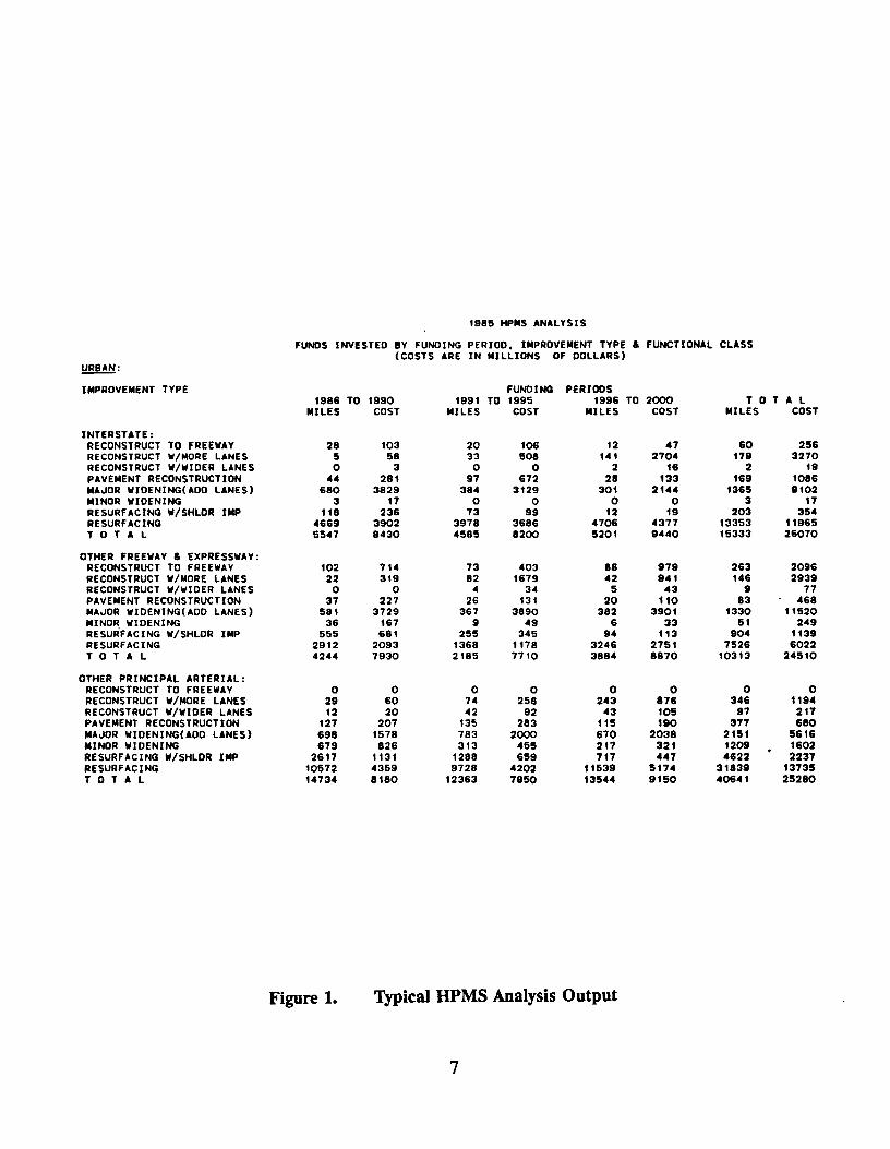
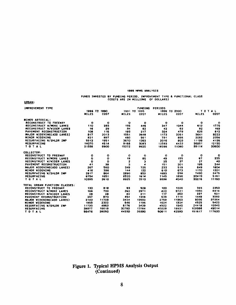
The HPMS Analytical Process was used to analyze the funding and performance characteristics under each scenario, for urban and rural areas, for six functionally classified systems, for eleven improvement types. Figure 1 shows a typical output from one of the analyses (referred to as Strategy 1 under high growth scenario for the US on p. 37 of this report) performed by the researchers at TTI.

AASHTO's Bottom Line

To provide background on the current level of highway, road, and bridge expenditures in the United States, the Bottom Line report includes a summary of expenses for the year 1985, the last year for which detailed expenditures were available at the time they published their report in September, 1988. This table is reproduced here as Table 1.

The AASHTO Bottom Line report generated estimates of highway investment needs for several scenarios, which are defined as follows [p.15]:

Current Investment Scenario - maintain spending at current levels.

Maintain Pavement Scenario - invest enough to keep pavements in an acceptable condition.

Maintain Service Scenario - limited investment is made in an attempt to maintain highway condition and service at current levels but some deterioration in service is allowed because of lack of investment to serve growing traffic.

6

1985 HPMS ANALYSIS

FUNDS INVESTED BY FUNDING PERIOD, IMPROVEMENT TYPE & FUNCTIONAL CLASS (COSTS ARE IN MILLIONS OF DOLLARS)

URBAN:

IMPROVEMENT TYPE FUNDING PERIODS 1986 TD 1990 1991 TD 1995 1996 TD 2000 T 0 T A L

MILES COST MILES COST MILES COST MILES COST

INTERSTATE: RECONSTRUCT TO FREEWAY 28 103 20 106 12 .. 7 60 256 RECONSTRUCT W/MORE LANES 5 58 33 508 141 2704 179 3270 RECONSTRUCT W/WIDER LANES 0 3 0 0 2 16 2 19 PAVEMENT RECONSTRUCTION 44 281 97 672 28 133 169 1086 MAJOR WIDENING(ADD LANES) 680 3829 384 3129 301 2144 1365 9102 MINOR WIDENING 3 17 0 0 0 0 3 17 RESURFACING W/SHLOR IMP 118 236 73 99 12 19 203 354 RESURFACING 4669 3902 3978 3686 4706 4377 13353 11965 T 0 T A L 5547 8430 4585 8200 5201 9440 15333 26070

OTHER FREEWAY & EXPRESSWAY: RECONSTRUCT TO FREEWAY 102 714 73 403 88 979 263 2096 RECONSTRUCT W/MORE LANES 22 319 82 1679 42 941 146 2939 RECONSTRUCT W/WJDER LANES 0 0 4 34 5 43 9 77 PAVEMENT RECONSTRUCTION 37 227 26 131 20 110 83 468 MAJOR WIDENING(ADD LANES) 581 3729 367 3890 382 3901 1330 11520 MINOR WIDENING 36 167 9 49 6 33 51 249 RESURFACING W/SHLDR IMP 555 681 255 345 94 113 904 1139 RESURFACING 2912 2093 1368 1178 3246 2751 7526 6022 T 0 T A L 4244 7930 2185 7710 3884 8870 10313 24510

OTHER PRINCIPAL ARTERIAL: RECONSTRUCT TO FREEWAY 0 0 0 0 0 0 0 0 RECONSTRUCT W/MORE LANES 29 60 74 258 243 876 346 1194 RECONSTRUCT W/WIDER LANES 12 20 42 92 43 105 97 217 PAVEMENT RECONSTRUCTION 127 207 135 283 115 190 377 680 MAJOR WIOENING(AOO LANES) 698 1578 783 2000 670 2038 2151 5616 MINOR WIDENING 679 826 313 455 217 321 1209 1602 RESURFACING W/SHLOR IMP 2617 1131 1288 659 717 447 4622 2237 RESURFACING 10572 4359 9728 4202 11539 5174 31839 13735 T 0 T A L 14734 8180 12363 7950 1354 .. 9150 40641 25280

Figure 1. Typical HPMS Analysis Output

7

1985 HPMS AHALYSlS

FUNOS INVESTED BY FUNDING PERIOD. IMPROVEMENT TVPE (COSTS ARE IN MILLIONS OF DOLLARS)

URBAN:

IMPROVEMENT TYPE FUNDING PERIODS 1986 TO 1990 1991 TO 1995 1996

Ml LES COST MILES COST MILES

MINOR ARTERIAL: RECONSTRUCT TO FREEWAY 0 0 0 0 0 RECONSTRUCT W/MORE LANES 110 285 155 446 347 RECONSTRUCT W/WIOER LANES 16 25 34 82 42 PAVEMENT RECONSTRUCTION 109 H6 193 2t7 324 MAJOR WIOENING(AOO LANES) 917 2013 1551 3848 1173 MINOR WIDENING 821 897 480 561 791 RESlJRFAClNG W/SHLDR IMP 5513 1951 3670 1382 2016 RESURFACING 14070 4614 9188 3083 13593 T 0 T A L 21556 9900 15272 9620 18286

COLLECTOR: RECONSTRUCT TO FREEWAY 0 0 0 0 0 RECONSTRUCT W/MORE LANES 0 0 18 BO 49 RECONSTRUCT W/WIOER LANES 0 0 2 3 25 PAVEMENT RECONSTRUCTION 41 39 3 4 151 MAJOR WlDENING(AOD LANES) 267 560 349 725 233 MINOR WIDENING 416 396 144 132 610 RESURFACING W/SHLDR IMP 29t7 96<1 2890 953 1683 RESURFACING 6754 1651 6520 '614 7145 T 0 T A L 10395 3610 9925 3510 9896

TOTAL URBAN FUNCTION CLASSES: RECONSTRUCT TO FREEWAY RECONSTRUCT W/MORE LANES RECONSTRUCT W/WIOER LANES PAVEMENT RECONSTRUCTION MAJOR WIOENING(AOO LANES) MINOR WIDENING RESURFACING W/SHLDR IMP RESURFACING T 0 T A L

130 818 93 509 100 f66 722 362 297' 822 28 48 82 2f1 117

357 870 454 1308 638 3143 11709 3.C3 .. 13592 2759 1955 2302 946 1196 1624

11720 4963 8176 3439 4522 38977 16619 30782 13764 40229 K476 38050 4030 36990 50811

Figure 1. Typical HPMS Analysis Output (Continued)

8

& FUNCTIONAL CLASS

TO 2000 T 0 T A L COST MILES COST

0 0 0 1044 6t2 '775

62 92 169 479 625 812

3361 3641 9222 898 2092 2356 803 11199 4136

4433 36851 12130 t 1080 55114 30600

0 0 0 155 67 235

37 27 40 201 195 244 519 849 1804 673 I 170 1201 558 7490 2 .. 75

1896 20419 5161 4040 30216 tH60

1026 323 2353 5721 t350 94'4

262 227 521 11'4 1449 3292

11963 9336 37264 1924 4S25 5422 1940 24418 10342

18631 109988 49014 42580 151617 117620

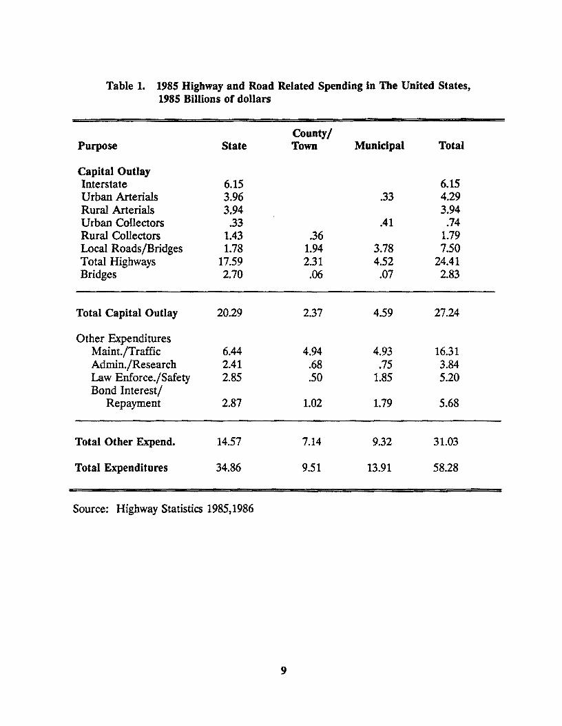
Table 1. 1985 Highway and Road Related Spending in The United States, 1985 Billions of dollars

County/ Purpose State Town Municipal Total

Capital Outlay Interstate 6.15 6.15 Urban Arterials 3.96 .33 4.29 Rural Arterials 3.94 3.94 Urban Collectors .33 .41 .74 Rural Collectors 1.43 .36 1.79 Local Roads/Bridges 1.78 1.94 3.78 7.50 Total Highways 17.59 2.31 4.52 24.41 Bridges 2.70 .06 .07 2.83

Total Capital Outlay 20.29 2.37 4.59 27.24

Other Expenditures Maint./Traffic 6.44 4.94 4.93 16.31 Admin./Research 2.41 .68 .75 3.84 Law Enforce./Safety 2.85 .50 1.85 5.20 Bond Interest/

Repayment 2.87 1.02 1.79 5.68

Total Other Expend. 14.57 7.14 9.32 31.03

Total Expenditures 34.86 9.51 13.91 58.28

Source: Highway Statistics 1985,1986

9

Constrained Improved Semce Scenario - attempt to meet deficiencies but limit widenings to the amount feasible without additional acquisition of right of way in new locations.

Improved Semce Scenario - make all investments required to meet identified deficiencies and respond to growth in travel demand.

The three last scenarios are considered the most realistic scenarios since they allow for investment to handle growing traffic and at least attempt to maintain current service. The annual highway investment required for each of these scenarios is shown in Table 2. Total annual investment for all roadways is shown in the last row of Table 2. For the last three scenarios, this cost ranges from $26.5 billion to $46.4 Billion. This does not include investment needs for local roads and for bridges. It also does not include costs for maintenance, traffic controls, administration, etc.

The AASHTO report does not attempt to provide a benefit-cost analysis or a rate-of­return analysis of the different investment scenarios, but a summary of a weighted index is given for each highway system for each scenario. This weighted index is an overall index that is based on how well highways in the United States are rated in terms of service (a measure of congestion), what condition they are in (especially how rough and deteriorated the pavements are), and how safe they are (as measured by number and severity of accidents). A perfect roadway would be rated to have a composite index of 100 in this rating procedure and the worst score would be zero. Table 3 shows the change in the composite index, in percent, weighted by daily vehicle miles traveled, for the different highway systems for each investment scenario. The first four scenarios have mainly negative numbers showing that these scenarios will show a deterioration in overall service, even though the Constrained Improved Scenario does show some improvement on most rural highways. The last scenario, Improved Service, shows improvement in almost all categories.

One of the recurring questions that arises in any analysis that is based on the HPMS analysis technique is bow are lane mile requirements calculated and what are the needs for new lane miles, most of which will be needed in urban areas. The Bottom Line report includes estimates of the number of current lane miles in the United States in 1985, and estimates based on HPMS of the number of lane miles needed on roads that can be expanded in the existing right of way and number of lane miles needed on new rights of way and these are shown in Table 4. This table does not include existing or needed lane miles for the states of Indiana, L:>uisiana, Michigan, and Oklahoma because comparable data were not available. It is estimated that the number of lane miles required in the United States between years 1985 and 2005 are 75,400 lane miles on existing right of way and 102,200 on new locations.

The Constrained Improved Semce Scenario assumes investment is made for the lane miles needed on existing right of way and the Improved Semce Scenario assumes that enough investment is made to provide the lanes needed on both existing and new right of

10

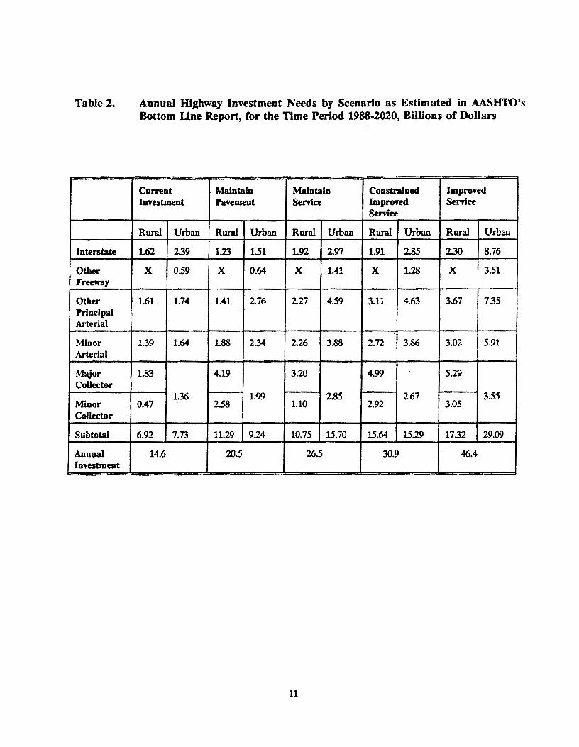
Table 2.

Interstate

Other Freeway

Other Principal Arterial

Minor Arterial

Major Collector

Minor Collector

Subtotal

Annual Investment

Annual Highway Investment Needs by Scenario as Estimated in AASHTO's Bottom Line Report, for the Time Period 1988-2020, Billions of Dollars

CWTent Maintain Maintain Constrained Improved Investment Pavement Senic:e Improved Senice

Service

Rural Urban Rural Urban Rural Urban Rural Urban Rural Urban

1.62 2.39 1.23 1.51 1.92 2.97 1.91 2.85 2.30 8.76

x 0.59 x 0.64 x 1.41 x 1.28 x 3.51

1.61 1.74 1.41 2.76 2.27 4.59 3.11 4.63 3.67 7.35

1.39 1.64 1.88 2.34 2.26 3.88 2.72 3.86 3.02 5.91

1.83 4.19 3.20 4.99 5.29

1.36 1.99 2.85 2.67 3.55 0.47 2.58 1.10 2.92 3.05

6.92 7.73 11.29 9.24 10.75 15.70 15.64 15.29 17.32 29.09

14.6 20.5 26.5 30.9 46.4

11

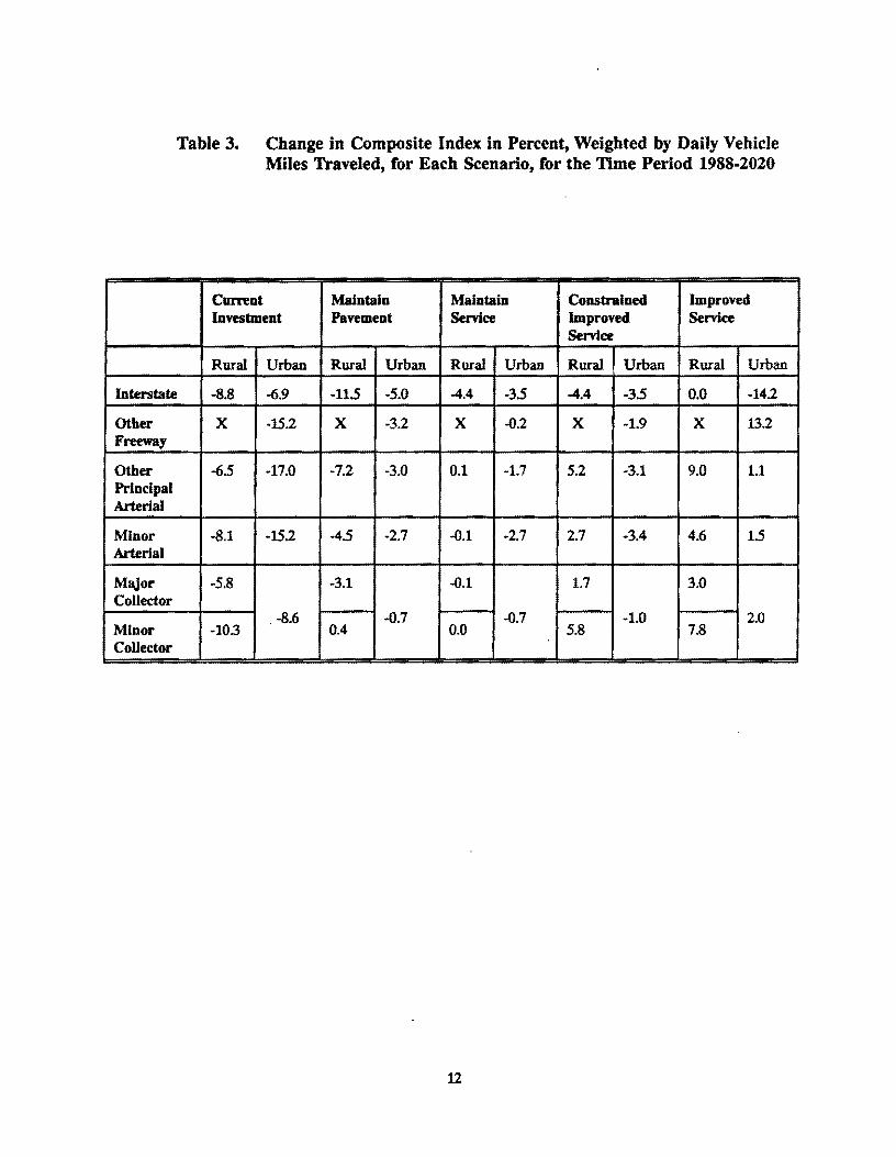
Table 3. Change in Composite Index in Percent, Weighted by Daily Vehicle Miles Traveled, for Each Scenario, for the Time Period 1988-2020

Cummt Maintain Maintain Constrained Improved Investment Pavement Senice Improved Senice

Se nice

Rural Urban Rural Urban Rural Urban Rural Urban Rural Urban

Interstate -8.8 -6.9 -11.5 -5.0 -4.4 -35 -4.4 -35 0.0 -14.2

Other x -15.2 x -3.2 x -0.2 x -1.9 x 13.2 Freeway

Other -6.S -17.0 -7.2 -3.0 0.1 -1.7 5.2 -3.1 9.0 1.1 Principal Arterial

Minor -8.1 -15.2 -4.S -2.7 -0.1 -2.7 2.7 -3.4 4.6 1.5 Arterial

Major -5.8 -3.1 -0.1 1.7 3.0 Collector

. -8.6 -0.7 -0.7 -1.0 2.0 Minor -103 0.4 0.0 5.8 7.8 Collector

12

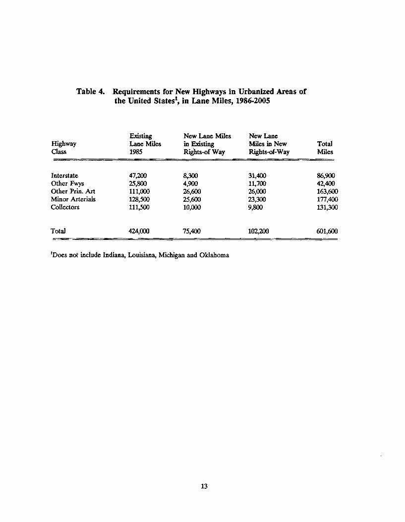
Table 4. Requirements for New Highways in Urbanized Areas of the United States1, in Lane Miles, 1986--2005

Existing New Lane Miles New Lane Highway Lane Miles in Existing Miles in New Class 1985 Rig'hts-of Way Rights-of· Way

Interstate 47;1iXJ 8,300 31,400 Other Fwys 25,800 4,900 11,700 Other Prin. Art 111,000 26,600 26,000 Minor Arterials 128,500 25,600 23,300 Collectors 111,500 10,000 9,800

Total 424,000 75,400 102,200

1Does not include Indiana, Louisiana, Michigan and Oklahoma

13

Total Miles

86,900 42,400 163,600 177,400 131,300

601,600

way. Providing these needed lanes is the main difference between the Maintain Senice Scenario and these two higher investment scenarios. Not providing these lanes leads to a considerable deterioration in the level of service on existing highways and is the principal reason for the deterioration in service shown in Table 3 for the lower levels of expenditure.

AASHTO's estimate of the total annual requirement for expenditures on highways, roads, and bridges is shown in Table 5. Note that the investment range shown for "low" and "high" are the annual highway investment estimates for the Maintain Service and Improved Senice scenarios from Table 2 ($26.5 billion and $46.4 billion, respectively). Table 6 shows total annual surface expenditure requirements for 1988-2020.

Based on the values in Table 5, AASIITO reaches the following conclusions:

*

*

Attempting to maintain service and the physical condition of the highway and road system at today's level through the year 2020 will require at least $80 billion per year. However, even at this funding level analyses show service is likely to deteriorate in some areas of the nation and on some highway systems.

An annual investment in highways and roads over the next 32 years [from 1988 to 2020] of approximately $100 billion is required to both maintain service and physical characteristics at today's level, and expand capacity to

accommodate expected future travel growth and improve current service levels.

It should be noted that the lower estimate of needs of $80 billion is the level of investment needed to maintain current service, the low level of the investment range for highways in Table 5, corresponding to the Maintain Senice scenario in Tables 2 and 3. Based on the levels of service in Table 3 for this scenario, it shows that if anything the AASHTO conclusion for service at the $80 billion level is overly optimistic. It also should be noted that this level of expenditure does not include any funds for new lanes, either on existing or new rights of way.

Although the AASHTO report does not provide a detailed analysis of road user costs, the following points are made:

1. The costs of the road are a minor, but absolutely crucial, part of total vehicle operating costs for private vehicle users. At about $400 a year per vehicle, road costs represent approximately 10 percent of total vehicle-related expenditures. It is this 10 percent that makes the nation's massive investment in freight, passenger transit, and personal use vehicles, and their supporting facilities, productive." (p.3)

14

Table S.

Program Area

Capital Outlays

Highways1

1...-0cal Roads Bridges

Subtotal

Other Outlays

Maint/Traffic J\dntln/Research Law Enf/Safety Debt Service

Subtotal

Total

AASHTO's Estimate of Annual Highway, Road, and Bridge Expenditure Requirements, 1988-2020, in Billions of Dollars

1988-2020 1985 Investment Range

Spending IA>w High

17.2 26.5 46.4 7.5 7.5 7.5 2.6 4.0 4.6

27.3 38.0 58.5

16.30 3.84 5.20 5.06

31.0 42.0 42.0

58.3 80.0 100.5

1Includes Interstate completion through 1991.

15

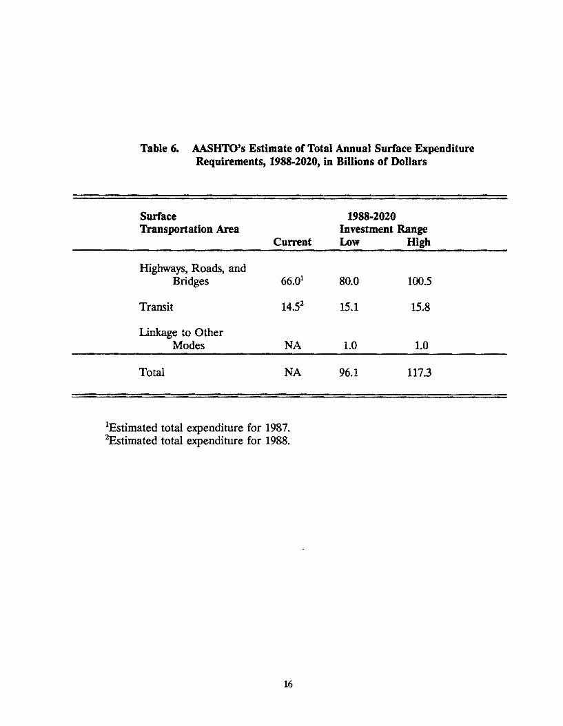
Table 6. AASHTO's Estimate or Total Annual Surface Expenditure Requirements, 1988-2020, in Billions or Dollars

Surface Transportation Area

Current

Highways, Roads, and Bridges 66.01

Transit 14.52

Linkage to Other Modes NA

Total NA

1Estimated total expenditure for 1987. 2Estimated total expenditure for 1988.

16

1988-2020 Investment Range Low High

80.0 100.5

15.1 15.8

1.0 1.0

96.1 117.3

2. In 1987, the total cost of the highway and road system cost users only 3.2 cents per vehicle mile (total expenditures of $66 billion divided by total miles of travel).

3. The AASHTO report also provides some estimates of increases in highway user costs from not providing a higher level of service (pp. 18-20). (The report also summarizes benefit estimates developed by FHWA in Workin& Paper 13, which is discussed in the following section of this chapter.)

FHWA's Workin1 Paper 13

In 1987 and 1988, as part of their evaluation of the status and future direction of the national highway program, the Federal Highway Administration developed a series of 19 working papers, with the general title of The Future National Hi1:hway Pro&ram - 1990 and Beyond; Workini Paper# 13 in this series has the subtitle of "Highway Performance and Investment Analysis" [2]. This working paper is important in several respects. First, it provides a comprehensive analysis of the level of investment and associated user costs for several highway investment scenarios. These analyses are of interest not only for the specific estimates but also because they provide the basis for the benefit/ cost ratios reported in AASIITO's Bottom Line report [1, p. 20] and also are the basis for the benefit and cost estimates for the rate-of-return analysis in the Congressional Budget Report [4].

Workin& Paper 13 uses the 1985 HPMS database for the United States. The HPMS analysis programs are used for four five-year funding periods encompassing the years from 1986 through 2005. The method used is summarized below [2, p. 3]:

Figure 2 is an abbreviated flow chart of the study procedure that was used. The first step was to establish five future funding scenarios between the years 1986 and 2005 that range from 20 percent below current funding to "full needs" funding. These investment scenarios were formulated for each highway functional class in rural, small urban, and urbanized areas. The scenarios were intended to encompass a reasonable range for investment policy consideration.

The different investment scenarios were used individually as inputs to the HPMS Needs/Investment Model, which estimates the future highway physical and operating conditions that will result from a given stream of available funding. The 1985 HPMS highway condition data set was used in the Needs/Investment Model to represent the base year highway and street conditions.

Next, the highway condition results from the Investment Model were translated by the HPMS Impact Model into user impacts (user operating costs,

17

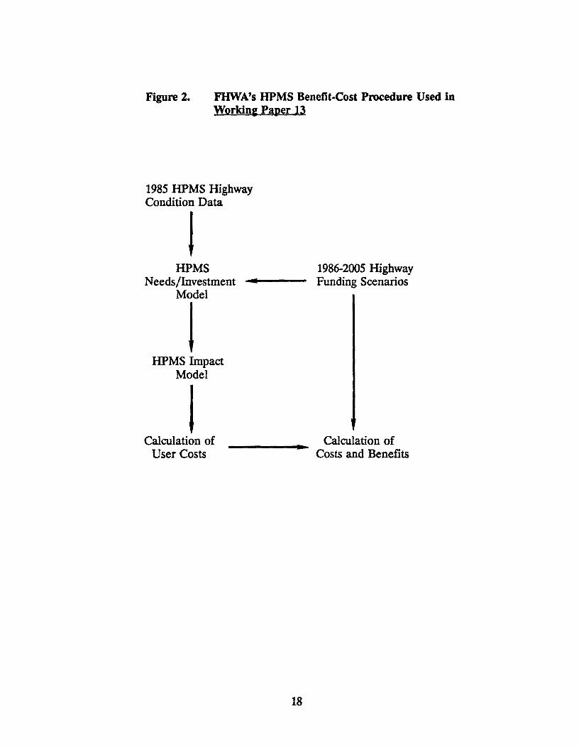
Figure 2. FHWA's HPMS Benefit-Cost Procedure Used in Workin1 Paper 13

1985 HPMS Highway Condition Data

l HPMS

Needs/Investment Model

l HPMS Impact

Model

' Calculation of User Costs

18

1986-2005 Highway Funding Scenarios

Calculation of Costs and Benefits

accident rates, and average travel speeds). These impacts were, in turn, converted into dollar estimates of actual user costs (operating costs, accident costs, and travel time costs) by applying the microcomputer spreadsheet algorithm that is used in FHW A's biennial "Needs Report" to Congress.

The steps above resulted in 20..year streams of highway investments and highway user costs at each funding level for each functional class in rural, small urban, and urbanized areas. Benefit-cost ratios were then determined by the following:

o calculating the annual difference between the highway expenditure under each pair of successive funding scenarios.

o calculating the annual difference between the resulting user costs for the two scenarios.

o calculating the 1985 new present values of the expenditure and user cost differences.

o dividing the discounted decrease in user costs (the benefits) by the discounted increase in expenditure (the costs) necessary to achieve them.

The resulting quotients for each pair of funding scenarios then represent an estimate of the reduction in user costs per dollar increase in highway investment.

Workin& Paper 13 is, as the name indicates, a working paper and does not attempt to provide a detailed analysis of all types of highway expenditures. It is of special interest in two respects, however: ( 1) it gives a description and analysis of several scenarios that are similar to those in the CBO study, and (2) the study does document in detail the procedure used to calculate user cost that are further used to calculate benefit·cost ratios for several investment levels. These benefit-cost ratios are shown here in Table 7.

The basic difference between it and the AASHTO Bottom Line analysis is that Workini Paper 13 uses a shorter time period and also uses scenarios that involve changing current funding by given percentages or that represent full needs.

National Council on Public Works Improvement's Fra&il~ Foundations Report

The National Council on Public Works Improvement (the "Council") was created by Public Works Improvement Act of 1984 (P.L 98-501) to assess the state of America's

19

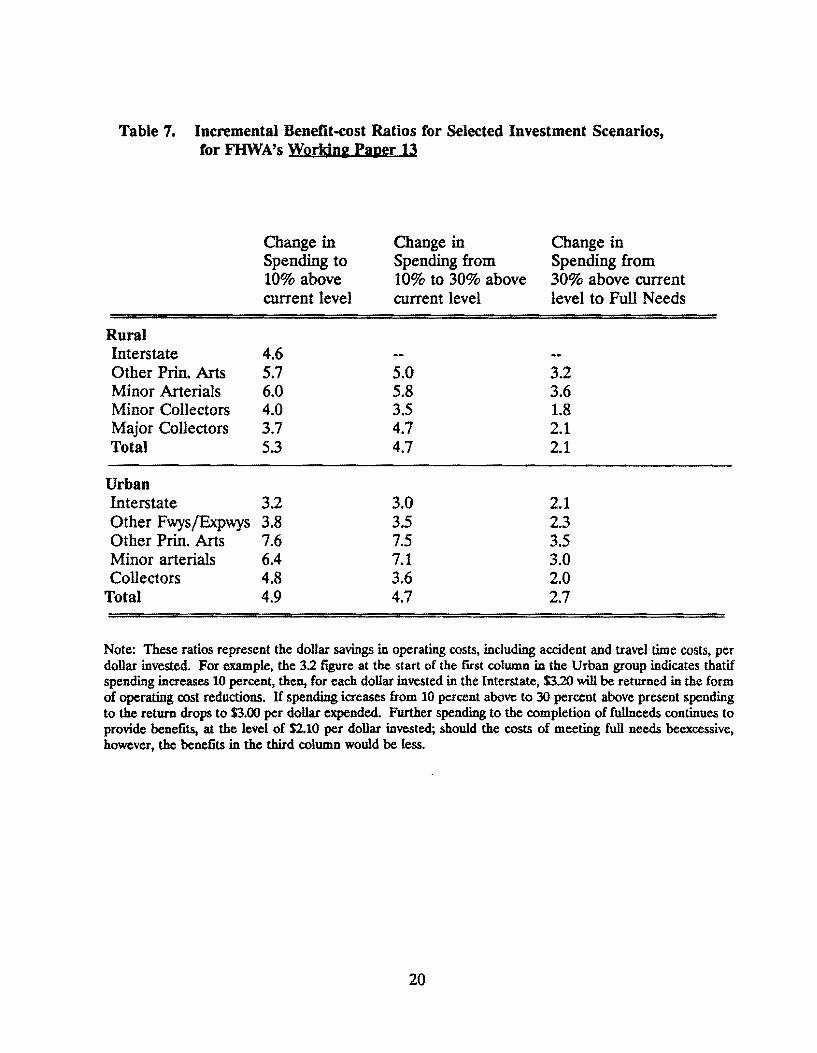
Table 7. Incremental Benefit-cost Ratios for Selected Investment Scenarios, for FHWA's Working Paper 13

Change in Change in Change in Spending to Spending from Spending from 10% above 10% to 30% above 30% above current current level current level level to Full Needs

Rural Interstate 4.6 Other Prin. Arts 5.7 5.0 3.2 Minor Arterials 6.0 5.8 3.6 Minor Collectors 4.0 3.5 1.8 Major Collectors 3.7 4.7 2.1 Total 5.3 4.7 2.1

Urban Interstate 3.2 3.0 2.1 Other Fwys/Expwys 3.8 3.5 2.3 Other Prin. Arts 7.6 7.5 3.5 Minor arterials 6.4 7.1 3.0 Collectors 4.8 3.6 2.0

Total 4.9 4.7 2.7

Note: These ratios represent the dollar savings in operating costs, including accident and travel time costs, per dollar invested. For example, the 3.2 figure at the start of the first column in the Urban group indicates thatif spending increases 10 percent, then, for each dollar invested in the Interstate, $3.20 will be returned in the form of operating cost reductions. If spending icreases from 10 percent above to 30 percent above present spending to the return drops to $3.00 per dollar expended. Further spending to the completion of fullneeds continues to provide benefits, at the level of $2.10 per dollar invested; should the costs of meeting full needs beexcessive, however, the benefits in the third column would be less.

20

infrastructure. The findings of the Council were published in February, 1988 in a final report to the President and Congress entitled Fra~le Foundations: A Report on America's Public Works. (A copy of P.L 98-501 is included as Appendix ill of the Council's report.) In addition, numerous background papers were prepared by the Council and others that provide additional related information. The Council's scope of study was very broad and included nine categories of public works and services: highways, roads, streets, and bridges; airports and airways; mass transit; intermodal transportation; water resources; water supply; wastewater management; solid waste; and hazardous waste. The primary concern of the present study was to review the Council's recommendations for highway investment needs as presented in the Council's final report

The Fra~le foundations report is quite different from the other three reports reviewed in this study in that it is very general in recommendations, as might be expected given the broad scope of the effort. The Council recommends evaluation of the performance of individual public works in four "performance measures": availability of physical assets, both public and private; delivery of service; quality of service; and economic performance.

The Council divides economic performance measures into two broad categories, economic efficiency and cost-effectiveness. The Council states that "the economic efficiency of a project or program is reflected by the excess of benefits over costs" whereas "cost­effectiveness provides simpler measures of services delivered per dollar spent" [3, p. 51].

In discussing economic efficiency, the Council notes that use of new present values calculations (benefits minus costs) can be used for evaluating economic efficiency and such evaluations are " ... analogous to private sector capital budgeting models where the firm's profit reflects net benefits." [3, p. 51]. Nevertheless, the Council notes that calculations of the economic efficiency of public works projects are not widely used:

[Performance analysis using benefits and costs] ... is not used systematically to evaluate governmental investments (except by the Corps of Engineers). It is difficult to use rate-of-return analysis to rank and choose among alternative government investments, in part, because it is difficult to define and value future public benefits. Moreover, using rate-of-return analysis for entire public works programs would require far greater data collection than is now used to support program decisions. Special factors also affect the assessment of government spending; for example, when considering the efficiency of the Interstate Highway System, national defense must be taken into account.

The time lag between expenditures and delivery of infrastructure services makes it difficult to measure program investment efficiency. Finally, an often overlooked measurement problem concerns the interaction of public and private investments. For example, the private efficiency of highway and aviation services depends on their use by privately owned and operated vehicles and aircraft. [3, p. 51.]

21

The Council notes that there have been more than a dozen national needs estimates since 1980, giving projections of all public works services. Three typical annual needs estimates are summarized in Table 8, representing studies by the Associated General Contractors, the CBO, and the Joint Economic Committee, as summarized by Peterson in a study prepared for the Council [40). The Council further says that needs estimates usually emphasize capital investment and do not evaluate possible changes in policy that could lead to reduced capital requirements. Also," ... studies must take care to control for inclusion of operation and maintenance expenditures, the periods of time over which estimates are made, the assumptions about economic growth and inflation built into the estimates, and the level of government and private involvement" [3, p. 38].

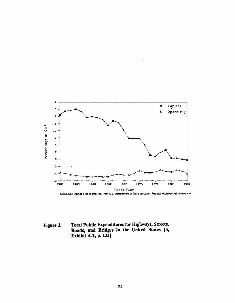
The Council presents data showing that the investment in public works in the United States has declined as a percent of Gross National Product; the decline in capital expenditures for highways, streets, roads, and bridges as a percent of GNP has been especially large, as shown in Figure 3, from the Council's final report [3, p. 132]. The Council's major recommendation for future investment in public works is:

... the Council recommends a national commitment, shared by all levels of government, the private sector, and the public, to vastly improve America's infrastructure. Such a commitment could require an increase of up to 100 percent in the amount of capital the nation invests each year in new and existing public works. In 1985, this amount was approximately $45 billion.

CBO New Directions in Public Works

The Congressional Budget Office prepared a critique of the Council's FraW:Ie Foundations report. A major point on which the CBO disagreed with the Council's finding on highways investment needs is about the availability of data for calculating economic performance measures for highway investment. The CBO proceeded to use data developed by FHWA, using the HPMS output based on 1985 data tapes to develop internal rates of return for total and marginal (or incremental) investment for different investment scenarios.

The internal rate of return represents the average earning power of the money used in a project over its life. It serves as a useful measure of how much a project is worth. The higher the internal rate of return, the higher the return of the dollar investment. It is equal to the discount rate that makes the net present value equal zero and is calculated as follows.

22

Table 8. Three National Needs Studies: Comparison of Annual Capital Investment Requirements, in Billions of 1982 Dollars

Infrastructur~ Cat~~Qll: AGC Stud)'.: CBO Stud:t me Stua:t (19 yr avge.)1 (1983-1990) (1983·2000)

Highways and bridges $ 62.82 $ 27.2 $ 40.0

Other transportation (mass transit, railroa~ airports, ports, locks, waterways )3

17.5 11.1 9.9

Drinking water 6.9 7.7 5.3

Wastewater treatment 25.4 6.6 9.1

Drainage _i2 NA 4

Total $ 118.2 $ 52.6 $ 64.3

1The time frame for addressing needs varied by specific infrastructure category from five to 25 years. 2Highways only. Bridges were estimated separately at an additional, one-time repair cost of $51. 7 billion. 3Needs for locks and waterways were not available from the JEC study; and needs for railroads were not available from the CBO study. 4Included under wastewater treatment.

SOURCE: George Peterson, et. al., Infrastructure Needs Studies: A Cridque, a paper prepared for the National Council on Public Works Improvement by The Urban Institute, July 1, 1986.

23

0... z u

, , ~ 13

l.Z v-ll

1.0

.9

.8

.7

.6

\ \ • •

Fiscal Year

• C~p1tal I Opr.!rnling 1

SOURCE: Apogee Research Inc. from U.S. Department of Transportation, Federal Highway Administration

Figure 3. Total Public Expenditures for Highways, Streets, Roads, and Bridges in the United States [3, Exhibit A-2, p. 132]

24

26 16

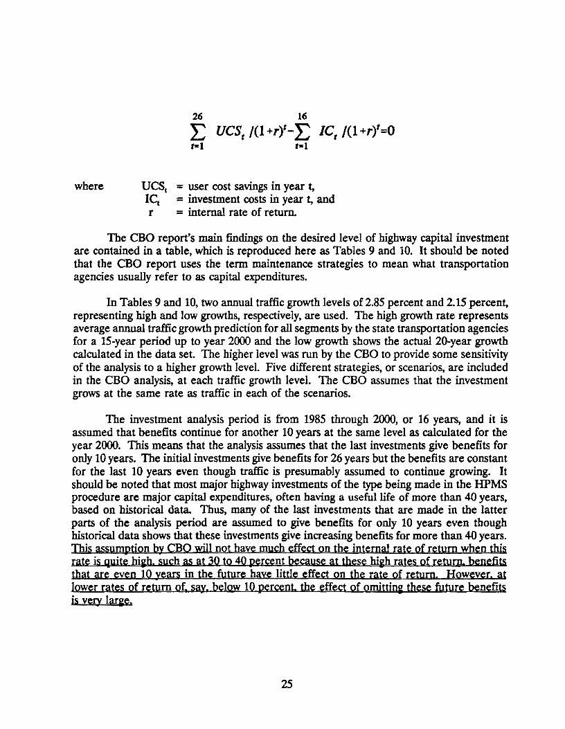
L UCS, /(1 +r)'-L JC, /(1 +r)'=O ~1 ~1

where ucst = user cost savings in year t, ICi = investment costs in year t, and r = internal rate of return.

The CBO report's main findings on the desired level of highway capital investment are contained in a table, which is reproduced here as Tables 9 and 10. It should be noted that the CBO report uses the term maintenance strategies to mean what transportation agencies usually refer to as capital expenditures.

In Tables 9 and 10, two annual traffic growth levels of 2.85 percent and 2.15 percent, representing high and low growths, respectively, are used. The high growth rate represents average annual traffic growth prediction for all segments by the state transportation agencies for a 15-year period up to year 2000 and the low growth shows the actual 20-year growth calculated in the data set. The higher level was run by the CBO to provide some sensitivity of the analysis to a higher growth level. Five different strategies, or scenarios, are included in the CBO analysis, at each traffic growth level. The CBO assumes that the investment grows at the same rate as traffic in each of the scenarios.

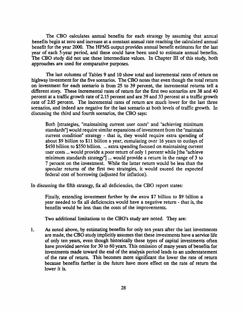
The investment analysis period is from 1985 through 2000, or 16 years, and it is assumed that benefits continue for another 10 years at the same level as calculated for the year 2000. This means that the analysis assumes that the last investments give benefits for only 10 years. The initial investments give benefits for 26 years but the benefits are constant for the last 10 years even though traffic is presumably assumed to continue growing. It should be noted that most major highway investments of the type being made in the HPMS procedure are major capital expenditures, often having a useful life of more than 40 years, based on historical data. Thus, many of the last investments that are made in the latter parts of the analysis period are assumed to give benefits for only 10 years even though historical data shows that these investments give increasing benefits for more than 40 years. This assumption by CBO will not have much effect on the internal rate of return when this rate is quite hi&}l. such as at 30 to 40 percent because at these high rates of return. benefits that are even 10 years in the future have little effect on the rate of return. However. at lower rates of return of. say. below 10 percent the effect of omittin& these future benefits is very lar~.

25

Table 9. Prospective Total Returns on Investment for Five Highway Maintenance Strategies, Under Low and High Traffic Growth, Using 1985 Prices

User Savings Investment Cost, 1985-2000 Per 1,000 Return om

Maintenance (In bWions of doUars)1 Vehicle Investment Strategy Cumulative Per Year Miler (Pen:ent)

Low Trame Growth (2.15 percent g:rowth a year in vehicle miles)

Maintain Current Spending 250 13 255 38 Maintain Current Highway

Conditions 279 15 316 38 Maintain Current User

Cost Levels 446 24 344 30 Achieve Minimum Standards 497 26 357 28 Fa: All Deficiencies 617 33 360 25

High Traffic Growth (2.85 percent growth a year in vehicle miles)

Maintain Current Spending 264 13 255 39 Maintain Current Highway

Conditions 315 16 316 38 Maintain Current User

Cost Levels 498 25 355 30 Achieve Minimum Standards 546 27 365 29 F'sx All Deficiencies 708 36 370 25

1Investment costs are assumed to increase in proportion to traffic growth, under each strategy. per year costs shown are for 1985, the first year of investment under each strategy.

The

2savings in this column show savings in 2000 when compared with the trend in transport costs that would follow from deteriorating road conditions under .a "No Maintenance" strategy.

SOURCE: Congressional Budget Office, based on data in Federal Highway Administration. The Status of the Nation's Hiahways: Conditions and Performance (June 1987).

26

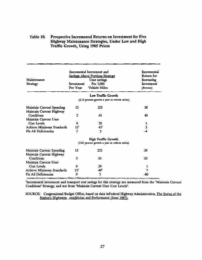
Table 10. Prospective Incremental Returns on Investment for Five Highway Maintenance Strategies, Under Low and High Traffic Growth, Using 1985 Prices

Maintenance Strategy

Maintain Current Spending Maintain Current Highway

Conditions Maintain Current User

Cost Levels Achieve Minimum Standards Fix: All Deficiencies

Maintain Current Spending Maintain Current Highway

Conditions Maintain Current User

Cost Levels Achieve Minimum Standards Fix All Deficiencies

Incremental Investment and Sayings Move Previous Strategy

Investment Per Year

User savings Per 1,000

Vehicle Miles

Low Trame Growth (2.15 pen:cnt growth a year in vehicle miles}

13

2

9 11• 7

255

61

28 411

3

High Traffic Growth (2.85 pen:cnt growth a year in vehicle miles)

13

3

9 111

9

255

61

39 491

5

Incremental Return for Increasing Investment (Percent)

38

40

1 3

4

39

33

1 7

-80

1Incremental investment and transport cost savings for this strategy are measured from the "Maintain Current Conditions" Strategy, and not from "Maintain Current User Cost Levels".

SOURCE: Congressional Budget Office, based on data inFederal Highway Administration, The Status of the Nation's Highways: conditioins and Performance (June 1987).

27

The CBO calculates annual benefits for each strategy by assuming that annual benefits begin at zero and increase at a constant annual rate reaching the calculated annual benefit for the year 2000. The HPMS output provides annual benefit estimates for the last year of each 5-year period, and these could have been used to estimate annual benefits. The CBO study did not use these intermediate values. In Chapter ill of this study, both approaches are used for comparative purposes.

The last columns of Tables 9 and 10 show total and incremental rates of return on highway investment for the five scenarios. The CBO notes that even though the total return on investment for each scenario is from 25 to 39 percent, the incremental returns tell a different story. These incremental rates of return for the first two scenarios are 38 and 40 percent at a traffic growth rate of 2.15 percent and are 39 and 33 percent at a traffic growth rate of 2.85 percent. The incremental rates of return are much lower for the last three scenarios, and indeed are negative for the last scenario at both levels of traffic growth. In discussing the third and fourth scenarios, the CBO says:

Both [strategies, "maintaining current user costs" and "achieving minimum standards"] would require similar expansions of investment from the "maintain current condition" strategy - that is, they would require extra spending of about $9 billion to $11 billion a year, cumulating over 16 years to outlays of $450 billion to $550 billion. ... extra spending focused on maintaining current user costs ... would provide a poor return of only 1 percent while [the "achieve minimum standards strategy"] ... would provide a return in the range of 3 to 7 percent on the investment While the latter return would be less than the specular returns of the first two strategies, it would exceed the expected federal cost of borrowing (adjusted for inflation).

In discussing the fifth strategy, fix all deficiencies, the CBO report states:

Finally, extending investment further by the extra $7 billion to $9 billion a year needed to fix all deficiencies would have a negative return - that is, the benefits would be less than the costs of the improvements.

Two additional limitations to the CBO's study are noted. They are:

1. As noted above, by estimating benefits for only ten years after the last investments are made, the CBO study implicitly assumes that these investments have a service life of only ten years, even though historically these types of capital investments often have provided service for 30 to 60 years. This omission of many years of benefits for investments made toward the end of the analysis period leads to an understatement of the rate of return. This becomes more significant the lower the rate of return because benefits farther in the future have more effect on the rate of return the lower it is.

28

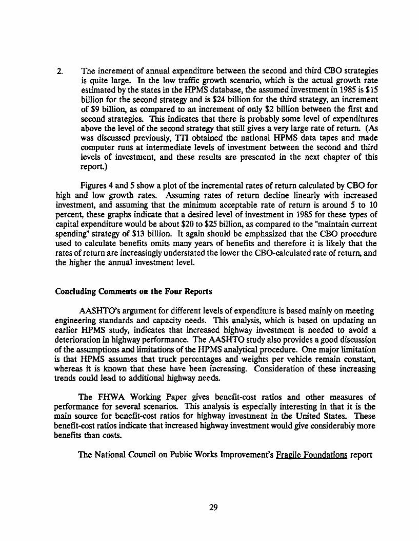
2. The increment of annual expenditure between the second and third CBO strategies is quite large. In the low traffic growth scenario, which is the actual growth rate estimated by the states in the HPMS database, the assumed investment in 1985 is $15 billion for the second strategy and is $24 billion for the third strategy, an increment of $9 billion, as compared to an increment of only $2 billion between the first and second strategies. This indicates that there is probably some level of expenditures above the level of the second strategy that still gives a very large rate of return. (As was discussed previously, TI1 obtained the national HPMS data tapes and made computer runs at intermediate levels of investment between the second and third levels of investment, and these results are presented in the next chapter of this report.)

Figures 4 and 5 show a plot of the incremental rates of return calculated by CBO for high and low growth rates. Assuming rates of return decline linearly with increased investment, and assuming that the minimum acceptable rate of return is around 5 to 10 percent, these graphs indicate that a desired level of investment in 1985 for these types of capital expenditure would be about $20 to $25 billion, as compared to the "maintain current spending" strategy of $13 billion. It again should be emphasized that the CBO procedure used to calculate benefits omits many years of benefits and therefore it is likely that the rates of return are increasingly understated the lower the CBO-calculated rate of return, and the higher the annual investment level.

Concluding Comments on the Four Reports

AASHTO's argument for different levels of expenditure is based mainly on meeting engineering standards and capacity needs. This analysis, which is based on updating an earlier HPMS study, indicates that increased highway investment is needed to avoid a deterioration in highway performance. The AASHTO study also provides a good discussion of the assumptions and limitations of the HPMS analytical procedure. One major limitation is that HPMS assumes that truck percentages and weights per vehicle remain constant, whereas it is known that these have been increasing. Consideration of these increasing trends could lead to additional highway needs.

The FHWA Working Paper gives benefit-cost ratios and other measures of performance for several scenarios. This analysis is especially interesting in that it is the main source for benefit-cost ratios for highway investment in the United States. These benefit-cost ratios indicate that increased highway investment would give considerably more benefits than costs.

The National Council on Public Works Improvement's Fraiile Foundations report

29

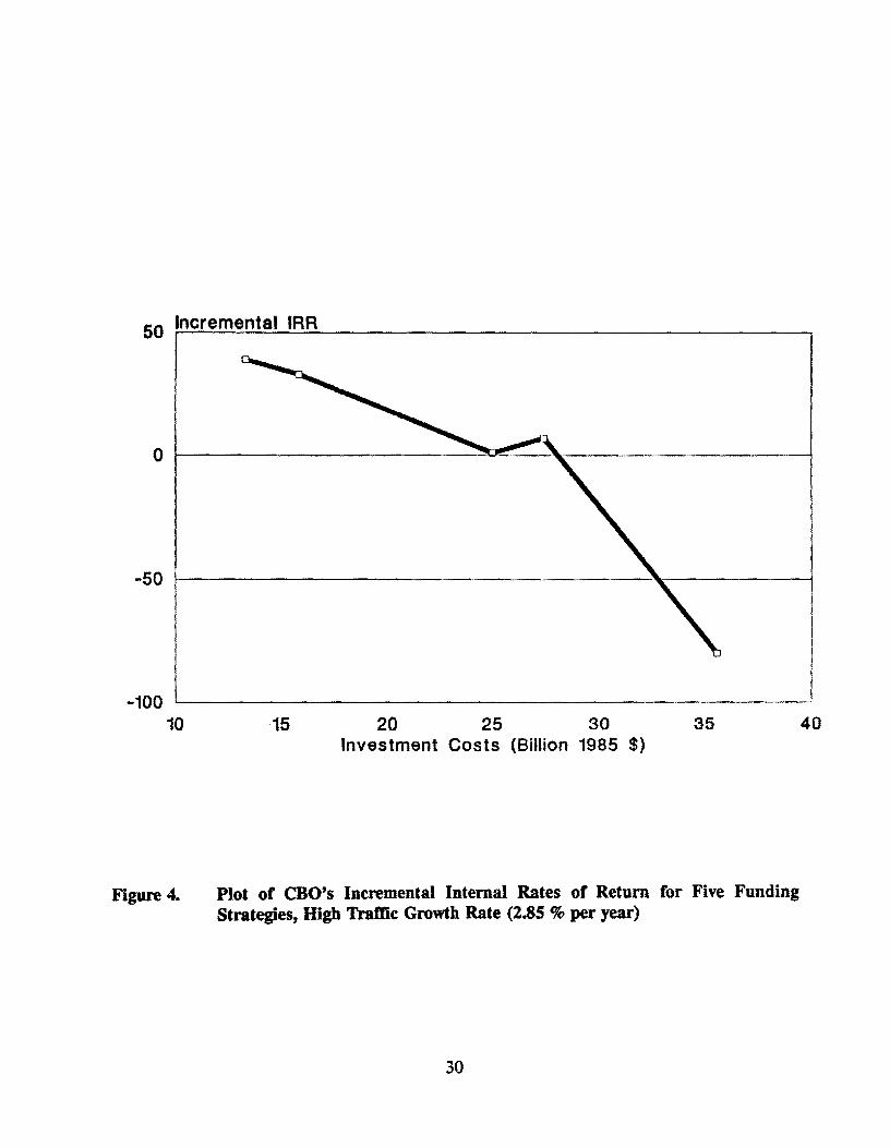
50 Incremental IRR

-100 10

Figure 4.

20 25 30 35 Investment Costs (Billion 1985 $)

Plot of CBO's Incremental Internal Rates of Return for Five Funding Strategies, High Traffic Growth Rate (2.85 % per year)

30

40

50 Incremental IRR

-10 ....._~~~~~~~~~~~~~~~~~~~~~~~~~---' 10

Figure S.

15 20 25 30 35 Investment Costs (Billion 1985 $)

Plot of CBO's Incremental Internal Rates of Return for Five Funding Strategies, Low Traffic Growth Rate (2.15 % per year)

31

is quite different from the other reports in that more emphasis is placed on the role of investment in public works in increasing economic growth in the economy. The Council states that investment in public works perhaps should be increased by 100 percent.

The CBO report is somewhat like the FHW A W orkini Paper 13 in terms of using an economic analysis, but the CBO puts the analysis in terms of rates of return instead of benefit-cost ratios.

The Congressional Budget Office is to be commended for its attempt to develop rates of return for highway investments. This analysis, together with that performed by FHW A in WorkinK Paper 13, promises to give a better indication of the economically justified level of expenditure on highways. In this respect, the analysis technique afforded by the HPMS data and analytical programs provides a tremendous advancement in the state of the art for evaluating needs for this important public works investment. This is undoubtedly the most comprehensive and accurate procedure available for making this type of analysis for any type of public work.

A limitation of the CBO study is that it did not develop rates of return for a wide enough range of investment levels. This weakens some of the report's conclusions. This is considered in detail in the following chapter of this report. It should be noted that:

1. The CBO uses relatively short (implicit) useful lives of from 10 to 25 years for highway investments that historically have been useful for from 30 to 60 years in many situations. The CBO's assumptions about useful lives may be relatively accurate for pavement overlays but for major capital expenditures such as adding lanes, widening, and improving facilities, these lives are too short. Using internal rate-of -return analysis, these errors in length of lives do not have much effect on rates of return that are hi~ but the lower the rate of return, the greater the effect. If the CBO had used longer service lives, they probably would not have calculated negative rates of return at the higher levels of investment.

2. Other estimation techniques are used that lead to an understatement of benefits, including relatively low values of time and costs for fatalities. By using final year estimates of benefits and not using values that are calculated by HPMS for intermediate years, the rates of return are understated.

32

III. EVALUATION AND CRITIQUE OF CBO ANALYSIS USING U.S. DATA

The principal analysis of highway investment in the CBO report is the estimation of rates of return for various levels and types of investment in highway facilities. The CBO estimates are based on several computer runs made by the FHW A using the HPMS analysis package. These FHW A computer runs were made to evaluate selected strategies and were not intended to cover a full range of investment levels. This resulted in some large gaps between the budget levels of the CBO scenarios. These gaps need to be filled to determine more precisely the level of highway investment that is justified on the basis of incremental internal rates of return (IRR's ).

TTI researchers contacted the CBO and FHW A and discussed the assumptions that were used in the development of rates of return that are presented in the CBO report. Also, the national HPMS data set was obtained from FHWA and the TTI copy of the HPMS analysis package was used to duplicate the runs made by FHWA and used by CBO in their report. Additional runs were made using different investment levels. The rate-of· return calculations on those investment levels were made in an attempt to duplicate the CBO results. Although there were some minor differences in the results of the TI1 results and the CBO report, probably because of small differences in the data that we obtained from FHW A or in the analysis programs, the TTI results were very similar to the CBO results when the same scenarios were studied.

Data Variation

Comparison of the results from data used in the analysis reported in the CBO report and from the data tape provided us by FHW A showed a slight variation. Thorough examination between the two sources has failed to reveal any concrete basis for the difference, based on the information available to us. Therefore, it is concluded that the 1985 HPMS data that FHWA used to run the analyses used by the CBO is slightly different from the data set that TTI received from FHW A Every year, each state submits its initial HPMS section data update at a certain date, and provides a final updated version later. The only available analysis that we could compare was the high traffic growth for the year 2000. The daily vehicle-miles traveled (DVM1j in the TI1 data set are consistently lower, ranging from as low as 2.6 percent in the urban other freeway/ expressway category to as high as 9.4 percent in the rural major collector category, giving an overall difference across all categories a 6.7 percent. Given the relatively small differences and the information available to us, it was decided that the HPMS analyses performed using the TTI data set should be legitimate for the purpose of the study.

The user costs and savings analyses in the CBO report are from results obtained in the FHW A report of the Secretary of Transportation to the United States Congress titled "'The Status of the Nation's Highways: Conditions and Performance" published in June 1987 [6]. The 1985 VMT are mentioned in Table ID·2 which match those in Hiihway Statistics.

33

However, it is not clear whether or not the analyses were run based on those VMT's as there is no mention of them in Chapter ill. As mentioned above, the only information we could compare is on DVMT from the HPMS output of year 2000 assuming a traffic growth of 2.85 percent. In our 1985 HPMS data tape, there are five missing states, namely Alaska, Indiana, LI>uisiana, Michigan, and Oklahoma. From the base year analysis, we have obtained DVMT by rural/urban and by functional class. It is found that our results match fairly closely with those published in Hi&hway Statistics for the same year after DVMT of the five missing states were deducted. Actually, the percentage differences between the HifUiway Statistics and ours range as low as -0.2 percent for the urban other freeway/ expressway category and as high as 5 percent in the urban collector category.

User Costs Calculation

From the Impact Analysis and Need Analysis in HPMS, operating costs and accident rates of the three accident types, namely fatal, injury, and property damage, per 1,000 VMT are output directly per 1,000 VMT for the last year of each analysis period. Using accident rate factors, the three accident rates are first converted into numbers of fatalities, numbers of nonfatal injuries, and number of damaged vehicles. By multiplying unit accident costs to the respective accident numbers, accident costs by accident type per 1,000 VMT are obtained, and the summation of the three types of unit accident costs yields the unit total accident costs per 1,000 VMT. Amounts of travel time for traveling 1,000 VMT for each of the seven vehicle types are calculated by dividing 1,000 VMT by the average traveling speed output from HPMS. By applying the vehicle mix, also an output item, and the respective unit travel time costs by vehicle type to the travel times by vehicle type, time costs per 1,000 VMT are obtained. Thus the three described user costs, operating costs, accident costs, and time costs, are in dollars per 1,000 VMT and are referred to as unit user costs. By multiplying DVMT, another HPMS output item, to the unit user costs gives daily user costs of the three categories which are further multiplied by 365 days to yield annual user costs by category. The summation of the three annual user costs categories results in total user costs. Since algorithms and defaults used in the development of user cost relationships in the current version of HPMS were based on 1980 data, procedures and factors used in updating to 1985 described in the report to Congress [6] are followed in this study. A brief discussion on each of these is presented below.

Operatina: Costs

Algorithms used for determining relationships between highway characteristics and the resulting vehicle operating costs output from the current HPMS Impact Model were based on 1980 data. Although revisions of updating unit costs to reflect current vehicle characteristics are being undertaken, these revisions were not available in time for this study. Therefore, the unit operating costs output from HPMS are updated to 1985 from 1980 using the Gross National Product implicit price deflators, with the resulting factor used being

34

1.2975.

Dme Costs

Unit costs for the seven vehicle types used by FHWA [6] were taken from "Time Values per Vehicle Hour for Seven Vehicle Oasses" [17] and were updated from 1980 to 1985 dollars using the Consumer Price Index (CPI). They are listed as follows:

Light Auto (Small Passenger Cars) Heavy Auto (Large Passenger Cars) Pickup/Van Single Unit Truck, 2-Axle Single Unit Truck, 3+-Axle Multi Unit Truck, 4-Axle Multi Unit Truck, 5+-Axle

Accident Costs

$ 7.23 7.23 8.81 9.76

13.00 14.30 14.30

Conversion factors to tum fatal, nonfatal injury, and PDO (property damage only) accident rates into numbers of fatalities, non-fatal injuries, and damaged vehicles in the CBO report were taken from "The Economic Cost to Society of Motor Vehicle Accidents" by the National Highway Traffic Safety Administration (NHfSA) [16] published in 1983 but based on 1980 data. These factors were further calibrated so that the HPMS base year analysis accident output would match the actual 1985 statistics for non-local highway accidents in the States included in the data set. These calibrated factors for the three accident types are as follows.

Fatalities per Fatal Accident 1.128 Nonfatal Injuries per Fatal Accident 1.081 Injuries per injury Accident 2.209 Damaged Vehicles per PDO 1. 700

The number of injuries consists of injuries from both fatal accidents and injury accidents. Unit accident costs adopted were from the same source and were updated to 1985 dollars using the CPI. They are listed as follows.

Per Fatality Per Nonfatal Injury Per Damaged Vehicle

$ 349,345 5,010

612

It is to be noted that the cost per fatality used here represents only the economic cost and not the full loss from accident death.

35

Trame Growth Rates

FHW A used two annual traffic growth rates of 2.85 percent and 2.15 percent in their 15 year (1985-2000) analyses, with the first referred to as high growth and the second as low growth. The high growth rate represents average annual traffic growth prediction for all segments by the state transportation agencies for a 15-year period up to year 2000 and the low growth shows the actual 20-year growth predicted in the data set. The use of two growth rates in the analyses provides some sensitivity of traffic growth. This study adopts the same two growth rates.

Funding Levels

A total of seven funding strategies were used, with Strategy 2 very close to the current budget of 13 billion 1985 dollars. Strategy 5 represents constrained full needs, Strategy 6 unconstrained full needs but with the number of lanes restricted to 12 at the maximum, while Strategy 7 represents unconstrained full needs with no lane restriction. Each funding level is assumed to grow over the 15 year period (1985-2000) at the same two traffic growth rates discussed above. For the high traffic growth rate consideration, Strategy 2 bas an initial investment cost of $12.28 billion in 1985, and a total cost of $245 billion (in 1985 dollars) for the 15 years period. Meanwhile the same strategy under low traffic prediction costs $12.04 billion for 1985 and $227 billion for the 15 years. The cumulative and initial funding levels for the seven strategies under both high and low growth are given in Table 11. With the exception of the three full needs strategies, funding allocation across functional classes used in this study is based initially on what FHW A used as shown in Table IV-17 [6], then further refined by switching funding from functional classes that have excess funding at the end of a period to classes that have high increases in operating costs or lower average speed from period to period. The final funding allocation by rural/urban and by functional class used in the analyses to produce the obtained user cost savings is shown in Tables 12a and 12b for high and low growth rates, respectively.

User Costs and Savings

Operating costs, accident costs, and time costs per 1,000 VMT for the end year of each analysis period are calculated for each functional class following the same procedures and updating factors used by FHW A [6] and described above. Each of them is then multiplied by the VMT for the respective year and functional class to yield the total operating costs, total accident costs, and total time costs for the end year of each period, and the sum of the three costs constitutes total user costs for the end year of each period for

36

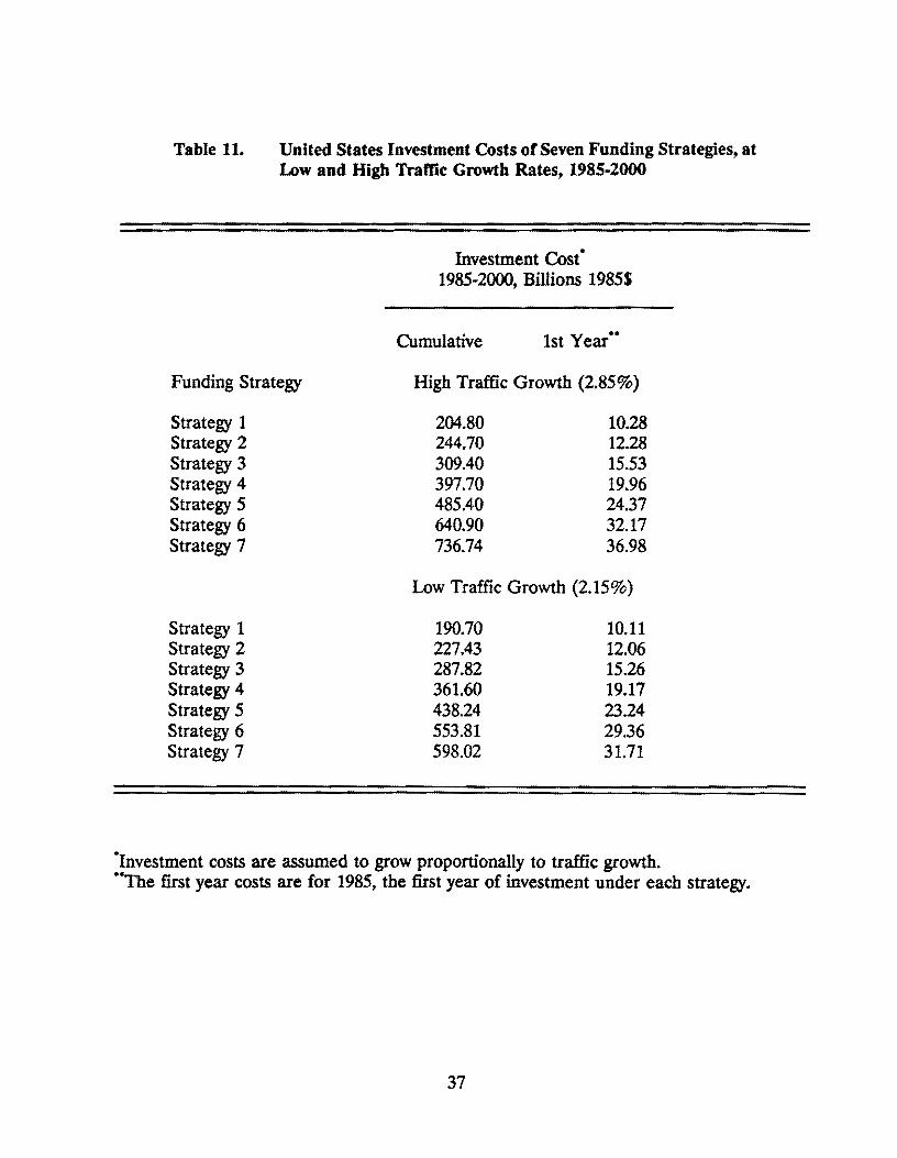
Table 11. United States Investment Costs of Seven Funding Strategies, at Low and High Trame Growth Rates, 1985-2000

Investment Cost· 1985-2000, Billions 1985$

Cumulative 1st Year ..

Funding Strategy High Traffic Growth (2.85%)

Strategy 1 Strategy 2 Strategy 3 Strategy 4 Strategy 5 Strategy 6 Strategy 7

Strategy 1 Strategy 2 Strategy 3 Strategy 4 Strategy 5 Strategy 6 Strategy 7

204.80 244.70 309.40 397.70 485.40 640.90 736.74

10.28 12.28 15.53 19.96 24.37 32.17 36.98

Low Traffic Growth (2.15%)

190.70 227.43 287.82 361.60 438.24 553.81 598.02

10.11 12.06 15.26 19.17 23.24 29.36 31.71

·1nvestment costs are assumed to grow proportionally to traffic growth. ··The first year costs are for 1985, the first year of investment under each strategy.

37

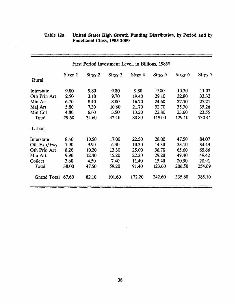
Table Ua. United States High Growth Funding Distribution, by Period and by Functional Class, 1985-2000

First Period Investment Level, in Billions, 1985$

Strgy 1 Strgy 2 Strgy 3 Strgy 4 Strgy 5 Strgy 6 Strgy 7 Rural

Interstate 9.80 9.80 9.80 9.80 9.80 10.30 11.07 0th Prin Art 2.50 3.10 9.70 19.40 29.10 32.80 33.32 Min Art 6.70 8.40 8.80 16.70 24.60 27.10 27.21 Maj Art 5.80 7.30 10.60 21.70 32.70 35.30 35.26 Min Col 4.80 6.00 3.50 13.20 22.80 23.60 23.55

Total 29.60 34.60 42.40 80.80 119.00 129.10 130.41

Urban

Interstate 8.40 10.50 17.00 22.50 28.00 47.50 84.07 0th Exp/Fwy 7.90 9.90 6.30 10.30 14.30 23.10 34.43 0th Prin Art 8.20 10.20 13.30 25.00 36.70 65.60 65.86 Min Art 9.90 12.40 15.20 22.20 29.20 49.40 49.42 Collect 3.60 4.50 7.40 11.40 15.40 20.90 20.91

Total 38.00 47.50 59.20 91.40 123.60 206.50 254.69

Grand Total 67.60 82.10 101.60 172.20 242.60 335.60 385.10

38

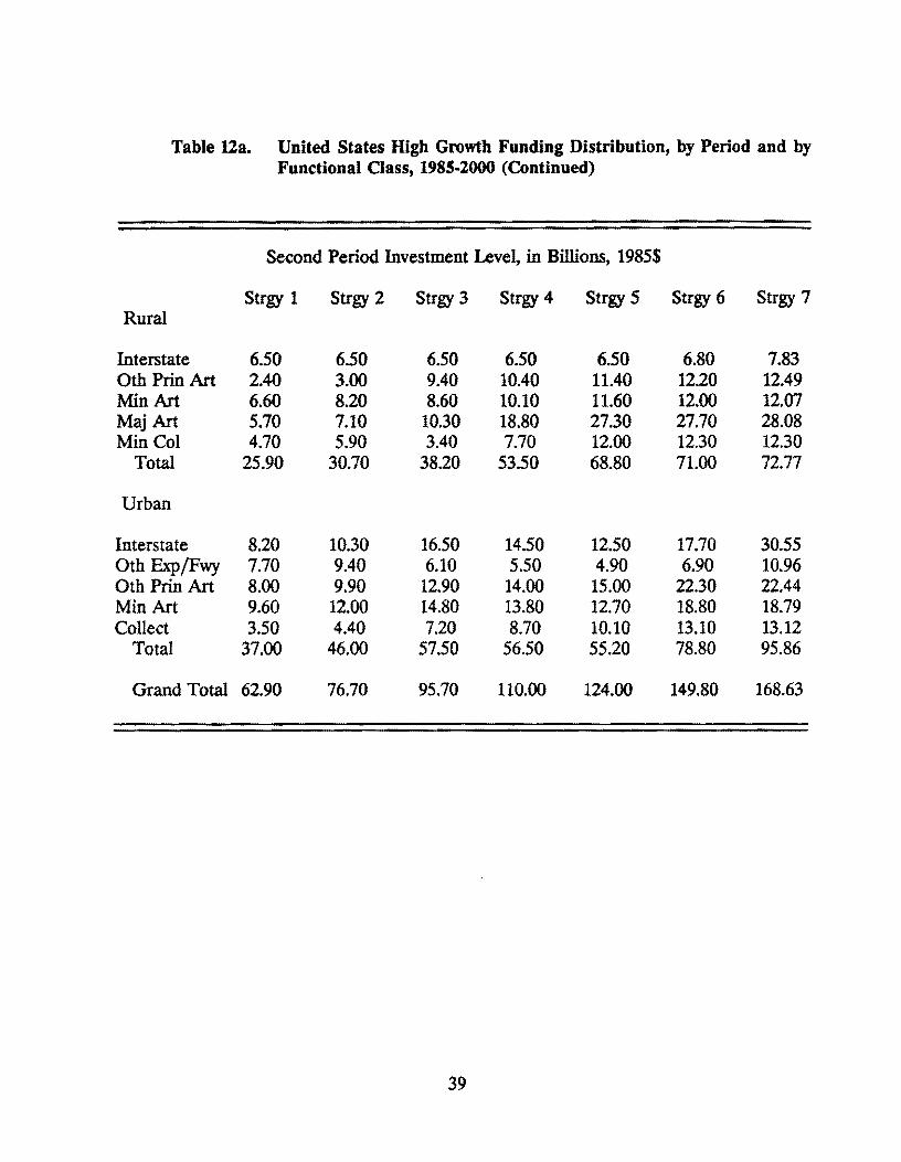
Table Ua. United States High Growth Funding Distribution, by Period and by Functional Class, 1985-2000 (Continued)

Second Period Investment Level, in Billions, 1985$

Strgy 1 Strgy 2 Strgy 3 Strgy 4 Strgy S Strgy 6 Strgy 7 Rural

Interstate 6.50 6.50 6.50 6.50 6.50 6.80 7.83 0th Prin Art 2.40 3.00 9.40 10.40 11.40 12.20 12.49 MinArt 6.60 8.20 8.60 10.10 11.60 12.00 12.07 Maj Art 5.70 7.10 10.30 18.80 27.30 27.70 28.08 Min Col 4.70 5.90 3.40 7.70 12.00 12.30 12.30

Total 25.90 30.70 38.20 53.50 68.80 71.00 72.77

Urban

Interstate 8.20 10.30 16.50 14.50 12.50 17.70 30.55 0th Exp/Fwy 7.70 9.40 6.10 5.50 4.90 6.90 10.96 0th Prin Art 8.00 9.90 12.90 14.00 15.00 22.30 22.44 Min Art 9.60 12.00 14.80 13.80 12.70 18.80 18.79 Collect 3.50 4.40 7.20 8.70 10.10 13.10 13.12

Total 37.00 46.00 57.50 56.50 55.20 78.80 95.86

Grand Total 62.90 76.70 95.70 110.00 124.00 149.80 168.63

39

Table Ila. United States High Growth Funding Distribution, by Period and by Functional Class, 1985-2000 (Continued)

1bird Period Investment Level, in Billions, 1985$

Strgy 1 Strgy 2 Strgy 3 Strgy 4 Strgy 5 Strgy 6 Strgy 7 Rural

Interstate 9.40 9.40 9.40 9.40 9.40 9.90 11.61 0th Prin Art 2.80 3.50 10.80 11.40 11.90 13.10 13.59 Min Art 7.60 9.40 9.80 9.70 9.50 10.40 11.02 Maj Art 6.50 8.20 11.90 13.60 15.30 15.80 15.82 Min Col 5.40 6.80 3.90 7.40 10.90 11.00 10.95

Total 31.70 37.30 45.80 51.50 57.00 60.20 62.99

Urban

Interstate 9.40 11.80 19.00 16.70 14.50 20.20 34.47 0th Exp/Fwy 8.90 6.50 7.00 6.80 6.60 10.90 19.71 0th Prin Art 9.20 11.40 14.90 16.90 18.80 29.50 31.22 Min Art 11.10 13.80 17.10 14.90 12.90 20.90 20.92 Collect 4.00 5.10 8.30 8.70 9.00 13.80 13.77

Total 42.60 48.60 66.30 64.00 61.80 95.30 120.02

Grand Total 74.30 85.90 112.10 115.50 118.80 155.50 183.01 Overall Inv 204.80 244.70 309.40 397.70 485.40 640.90 736.74

40

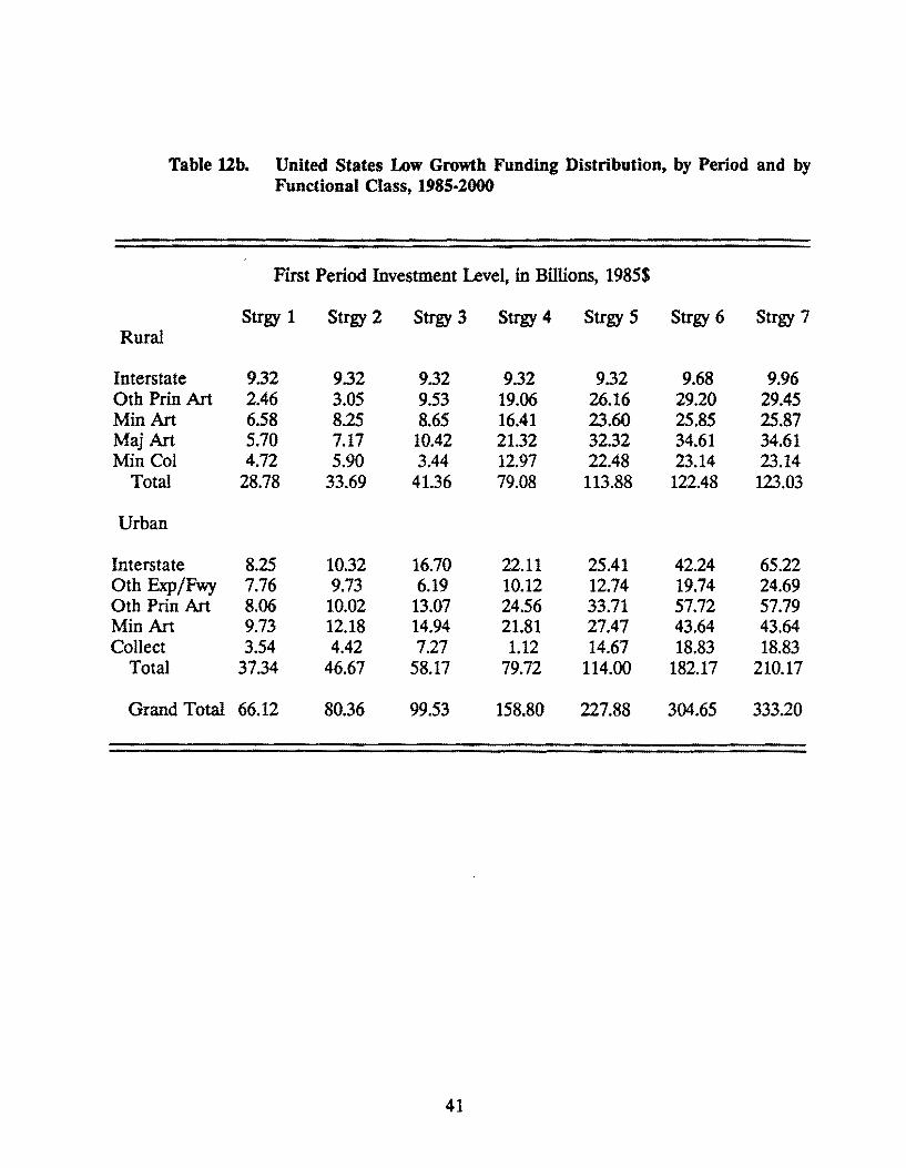
Table 12b. United States I.ow Growth Funding Distribution, by Period and by Functional Class, 1985·2000

First Period Investment Level, in Billions, 1985$

Strgy 1 Strgy 2 Strgy 3 Strgy 4 Strgy S Strgy 6 Strgy 7 Rural

Interstate 9.32 9.32 9.32 9.32 9.32 9.68 9.96 0th Prin Art 2.46 3.05 9.53 19.06 26.16 29.20 29.45 Min Art 6.58 8.25 8.65 16.41 23.60 25.85 25.87 Maj Art 5.70 7.17 10.42 21.32 32.32 34.61 34.61 Min Col 4.72 5.90 3.44 12.97 22.48 23.14 23.14

Total 28.78 33.69 41.36 79.08 113.88 122.48 123.03

Urban

Interstate 8.25 10.32 16.70 22.11 25.41 42.24 65.22 0th Exp/Fwy 7.76 9.73 6.19 10.12 12.74 19.74 24.69 0th Prin Art 8.06 10.02 13.07 24.56 33.71 57.72 57.79 Min Art 9.73 12.18 14.94 21.81 27.47 43.64 43.64 Collect 3.54 4.42 7.27 1.12 14.67 18.83 18.83

Total 37.34 46.67 58.17 79.72 114.00 182.17 210.17

Grand Total 66.12 80.36 99.53 158.80 227.88 304.65 333.20

41

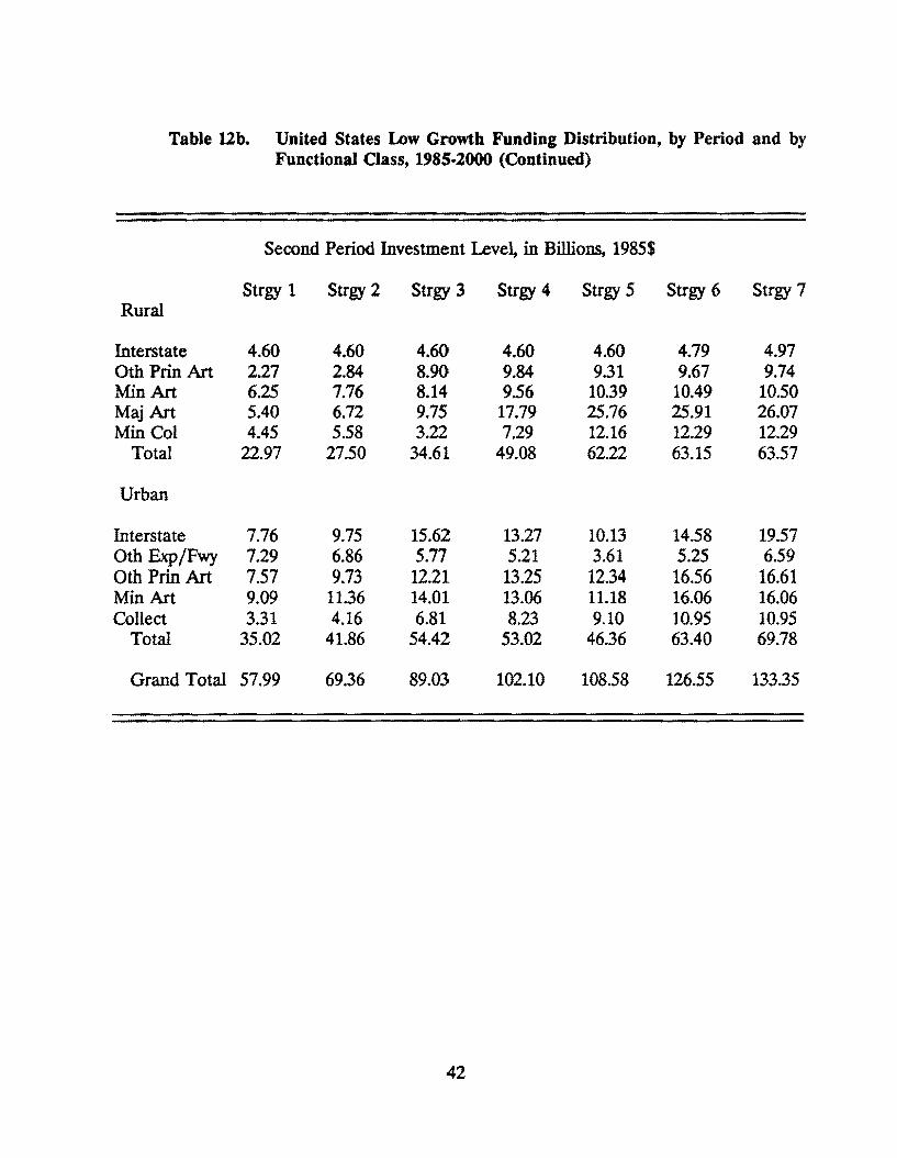
Table 12b. United States Low Growth Funding Distribution, by Period and by Functional Class, 1985·2000 (Continued)

Second Period Investment Level, in Billions, 1985$

Strgy 1 Strgy 2 Strgy 3 Strgy 4 Strgy 5 Strgy 6 Strgy 7 Rural

Interstate 4.60 4.60 4.60 4.60 4.60 4.79 4.97 0th Prin Art 2.27 2.84 8.90 9.84 9.31 9.67 9.74 Min Art 6.25 7.76 8.14 9.56 10.39 10.49 10.50 Maj Art 5.40 6.72 9.75 17.79 25.76 25.91 26.07 Min Col 4.45 5.58 3.22 7.29 12.16 12.29 12.29

Total 22.97 27.50 34.61 49.08 62.22 63.15 63.57

Urban

Interstate 7.76 9.75 15.62 13.27 10.13 14.58 19.57 0th Exp/Fwy 7.29 6.86 5.77 5.21 3.61 5.25 6.59 0th Prin Art 7.57 9.73 12.21 13.25 12.34 16.56 16.61 Min Art 9.09 11.36 14.01 13.06 11.18 16.06 16.06 Collect 3.31 4.16 6.81 8.23 9.10 10.95 10.95

Total 35.02 41.86 54.42 53.02 46.36 63.40 69.78

Grand Total 57.99 69.36 89.03 102.10 108.58 126.55 133.35

42

Table 12b. United States Low Growth Funding Distribution, by Period and by Functional Class, 1985-2000 (Continued)

Third Period Investment Level, in Billions, 1985$

Strgy 1 Strgy 2 Strgy 3 Strgy 4 Strgy 5 Strgy 6 Strgy 7 Rural

Interstate 8.07 8.07 8.07 8.07 8.07 8.33 8.79 0th Prin Art 2.56 3.20 9.88 10.43 8.99 9.74 9.79 Min Art 6.95 8.60 8.96 8.87 7.62 7.91 7.91 Maj Art 5.95 7.50 10.89 12.44 13.96 14.14 14.32 Min Col 4.94 6.22 3.57 6.77 9.64 9.42 9.42

Total 28.47 33.59 41.37 46.58 48.28 49.54 50.23

Urban

Interstate 8.60 10.79 14.62 10.84 10.85 14.25 19.87 0th Exp/Fwy 7.30 5.60 6.40 6.22 5.67 7.34 9.34 0th Prin Art 8.42 10.43 13.63 15.46 18.57 27.11 27.66 Min Art 10.15 12.62 15.64 13.63 10.49 14.22 14.22 Collect 3.66 4.67 7.59 7.96 7.92 10.15 10.15

Total 38.13 44.11 57.88 54.11 53.50 73.07 81.24

Grand Total 66.60 77.70 99.25 100.69 101.78 122.61 131.47 Overall Inv 190.71 227.42 287.81 361.59 438.24 553.81 598.02

43

each functional class. Total user costs for each strategy is the summation of total user costs of all functional classes and the unit total user costs in 1,000 VMT are obtained after dividing total user costs by the appropriate DVMT. Unit total user savings (in 1,000 VMT) for each strategy results when units total user costs of each strategy is compared to the 'Non­Maintain' strategy. Table 13 shows DVMT for all functional classes in both rural and urban for the two traffic growth rates output from HPMS Impact Analysis. In year 2000, if traffic grows annually at 2.85 percent (high growth rate), a total of 5,768 million DVMT would result as compared to 5,142 million DVMT for the low traffic growth scenario. Total user savings for 1990, 1995, and 2000 for each strategy under high and low growths are given in Table 14. Figure 6 illustrates the relationship between initial investment costs and user savings at the end of the three periods· under the high growth scenario. Incremental investment costs for the first year and incremental user savings for the years 1990, 1995, and 2000 are obtained separately when investment costs and user savings of one strategy are compared to those of the strategy with immediately higher funding level; these are shown in Table 15.

Internal Rates of Return

111 researchers used two methods of calculating the internal rate of return. The first method, which is the one used by the CBO, calculates user cost savings for the year 2000 and assumes that annual benefits begin in 1985 and grow at a constant annual rate to reach the annual savings for the year 2000 in the sixteenth year; it further assumes that annual benefits for an additional 10 years from 2001 to 2010 are the same as annual benefits in year 2000. The second method uses the HPMS user savings for the end years of each of the three periods and the benefits are calculated between those points assuming a constant growth rate. The savings of the last year in the last period (2000) are assumed constant over the next 10 years, the same as for the first method.

Incremental internal rates of return are calculated using the differential between investment costs and user savings between one strategy and the next higher funding level strategy. They represent the marginal returns of investments and are valuable information for planning decisions. Internal rates of return and incremental internal rates of return for each strategy under high and low growths for the two methods are presented in Table 16. The second method using user cost savings for the end years of the three periods shows higher internal rates of return than does the less accurate method used by CBO, under both high and low growths, within most of the investment range under study as demonstrated in Figures 7 and 8.

44

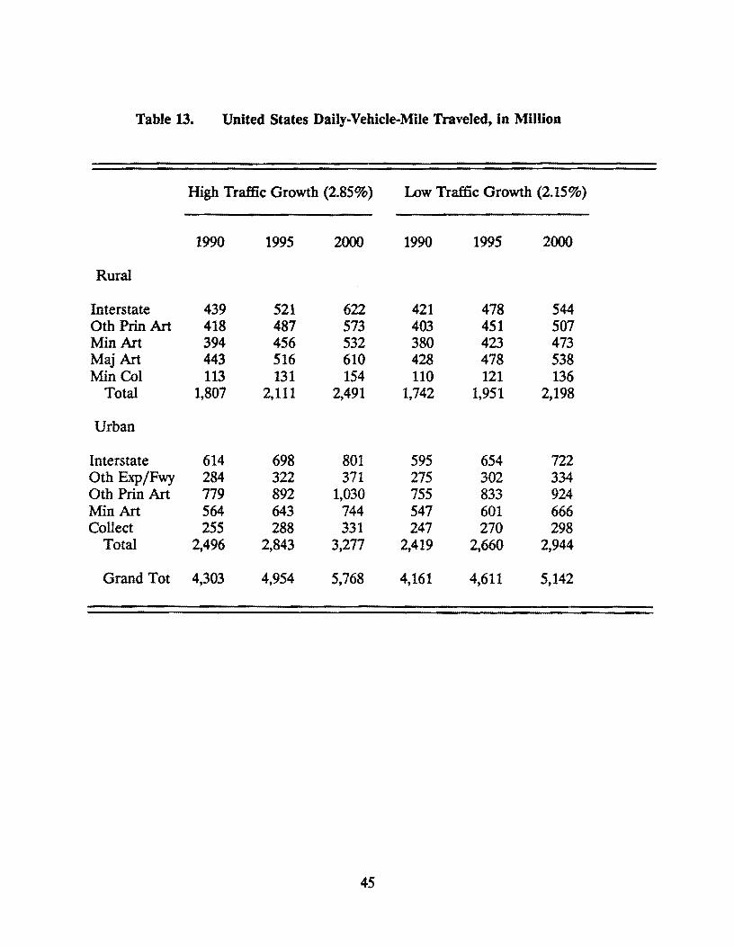
Table 13. United States Daily-Vehicle-Mile Traveled, in Million

High Traffic Growth (2.85%) Low Traffic Growth (2.15%)

1990 1995 2000 1990 1995 2000

Rural

Interstate 439 521 622 421 478 544 0th Prin Art 418 487 573 403 451 507 Min Art 394 456 532 380 423 473 Maj Art 443 516 610 428 478 538 Min Col 113 131 154 110 121 136

Total 1,807 2,111 2,491 1,742 1,951 2,198

Urban

Interstate 614 698 801 595 654 722 0th Exp/Fwy 284 322 371 275 302 334 0th Prin Art 779 892 1,030 755 833 924 Min Art 564 643 744 547 601 666 Collect 255 288 331 247 270 298

Total 2,496 2,843 3,277 2,419 2,660 2,944

Grand Tot 4,303 4,954 5,768 4,161 4,611 5,142

45

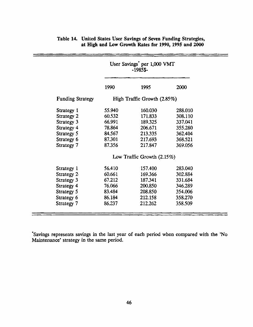
Table 14. United States User Savings of Seven Funding Strategies, at High and Low Growth Rates for 1990, 1995 and 2000

Funding Strategy

Strategy 1 Strategy 2 Strategy 3 Strategy 4 Strategy 5 Strategy 6 Strategy 7

Strategy 1 Strategy 2· Strategy 3 Strategy 4 Strategy 5 Strategy 6 Strategy 7

User Savings· per 1,000 VMT -1985$-

1990 1995 2000

High Traffic Growth (2.85%)

55.940 160.030 288.010 60.532 171.833 308.110 66.991 189.325 337.041 78.864 206.671 355.280 84.567 213.335 362.404 87.301 217.693 368.521 87.356 217.847 369.056

Low Traffic Growth (2.15 % )

56.410 157.400 283.040 60.661 169.366 302.884 67.212 187.341 331.684 76.066 200.850 346.289 83.484 208.850 354.006 86.184 212.158 358.270 86.237 212.262 358.509

·savings represents savings in the last year of each period when compared with the 'No Maintenance' strategy in the same period.

46

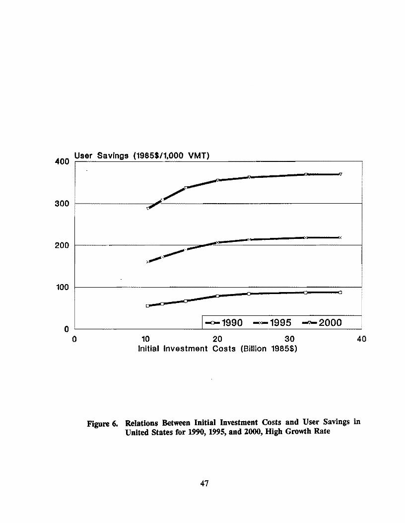
400 User Savings (1985$/1.000 VMT)

300

200

100

0 0

7 'ii rrfJi

,,,,-R

/''-~· ,

>..,,~-----

,,,,. ... ..0 <J D

~ ..-P'2

l-ci-1990 -x-1995 ~2000

10 20 30 40 Initial Investment Costs (Billion 1985$)

Figure 6. Relations Between Initial Investment Costs and User Savings in United States for 1990, 1995, and 2000, High Growth Rate

47

Table 15. United States Incremental Investment Costs and Incremental User Savings of Seven Funding Strategies, at High and Low Growth Rates for 1990, 1995, and 2000

Incremental User Savings· per 1,000 VMT

Incremental -1985$-Investment -Billion 1985$-1st Year •• 1990 1995 2000

Funding Strategy High Traffic Growth (2.85%)

Strategy 1 10.28 55.940 160.030 288.010 Strategy 2 2.00 4.592 11.803 20.100 Strategy 3 3.25 6.459 17.492 28.931 Strategy 4 4.43 11.873 17.346 18.239 Strategy 5 4.40 5.703 6.664 7.124 Strategy 6 7.81 2.734 4.358 6.117 Strategy 7 4.81 .055 .154 .535

Low Traffic Growth (2.15%)

Strategy 1 10.11 56.000 158.000 283.000 Strategy 2 1.95 4.251 11.966 19.844 Strategy 3 3.20 6.551 17.975 28.800 Strategy 4 3.91 8.854 13.509 14.605 Strategy 5 4.06 7.418 8.000 7.717 Strategy 6 6.13 2.700 3.308 4.264 Strategy 7 2.34 .053 .104 .239

·savings represents savings in the last year of each period when compared with the 'No Maintenance' strategy in the same period . .. The first year costs are for 1985, the first year of investment under each strategy.

48

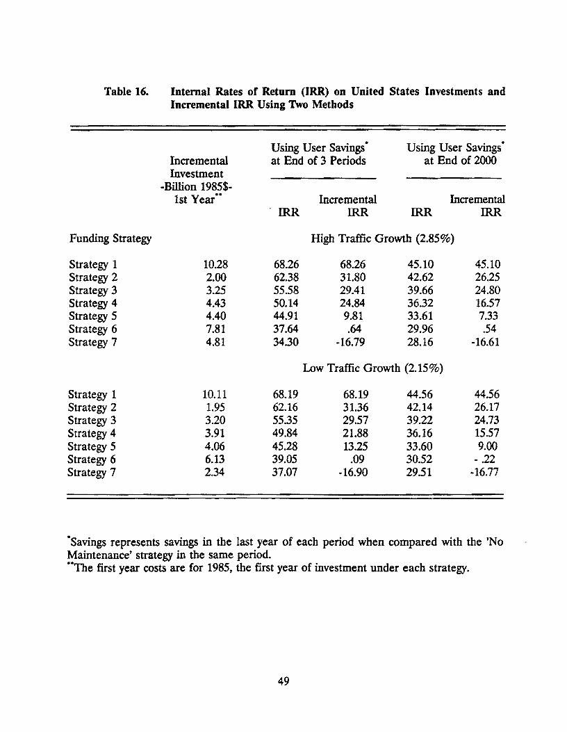
Table 16. Internal Rates of Return (IRR) on United States Investments and Incremental IRR Using Two Methods

Using User Savings • Using User Savings .

Incremental at End of 3 Periods at End of 2000 Investment

-Billion 1985$-1st Year •• Incremental Incremental

. IRR IRR IRR IRR

Funding Strategy High Traffic Growth (2.85%)

Strategy 1 10.28 68.26 68.26 45.10 45.10 Strategy 2 2.00 62.38 31.80 42.62 26.25 Strategy 3 3.25 55.58 29.41 39.66 24.80 Strategy 4 4.43 50.14 24.84 36.32 16.57 Strategy 5 4.40 44.91 9.81 33.61 7.33 Strategy 6 7.81 37.64 .64 29.96 .54 Strategy 7 4.81 34.30 -16.79 28.16 -16.61

Low Traffic Growth (2.15%)

Strategy 1 10.11 68.19 68.19 44.56 44.56 Strategy 2 1.95 62.16 31.36 42.14 26.17 Strategy 3 3.20 55.35 29.57 39.22 24.73 Strategy 4 3.91 49.84 21.88 36.16 15.57 Strategy 5 4.06 45.28 13.25 33.60 9.00 Strategy 6 6.13 39.05 .09 30.52 - .22 Strategy 7 2.34 37.07 -16.90 29.51 -16.77

"Savings represents savings in the last year of each period when compared with the 'No Maintenance' strategy in the same period . .. The first year costs are for 1985, the first year of investment under each strategy.

49

-50

-100 0

' ' -a-TTI Using User Savings of 3 Periods -~ TTI Using User Savings of Year 2000 -c- CBO

Figure 7.

10 20 30 Initial Investment Costs (Billion 1985$)

United States Incremental Internal Rates of Return for Seven Funding Strategies, High Trame Growth Rate (2.85 % per year)

50

40

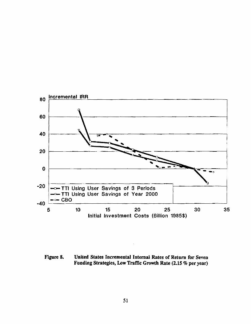
80 Incremental IRA,:__ __________ ~-----------.

40 i-----

·20 .....a-TTI Using User Savings of 3 Periods -"-TTI Using User Savings of Year 2000 -o- CBO

-40 L--~-~--------------'--~----~ 5 10 15 20 25 30 35

Figure 8.

Initial Investment Costs (Billion 1985$)

United States Incremental Internal Rates of Return for Seven Funding Strategies, Low Trame Growth Rate (2.15 % per year)

51

Summary and Concluding Comments

As noted previously in Chapter Il, the CBO report emphasizes the point that the "maintain current user cost levels" strategy (corresponding to first year spending of about $24 billion) gives an incremental internal rate of return (IRR) of only one percent. This incremental IRR is calculated for the $11 billion increment of spending in going from annual spending of $13 billion to $24 billion. This strategy corresponds roughly to strategy 5 in Table 16; Strategy 5 in the TI1 runs has $24.37 billion in the high traffic growth scenario and $23.24 billion in the low traffic growth scenario; however, the TI1 computer runs use smaller increments so that intermediate investment levels can be evaluated.

In the TI1 runs, Strategy 5 shows incremental rates of return of 7.33 percent and 9.00 percent for the two growth levels (last column of Table 16) if the CBO method of calculating benefits is used, with estimation of user savings based on benefits at the end of year 2000. If user savings at the end of 3 periods are used, the corresponding rates of return for Strategy 5 are 9.81 percent for high traffic growth and 13.25 percent for low traffic growth.

It should be noted that, although the CBO report presents rates of return for two traffic growth rates, the actual traffic growth rates that appear in the HPMS data base are what the CBO refers to as the "low growth rates"; these low growth rates are the actual predicted traffic growth rates. Therefore, using the actual predicted t~affic growth rates, and using the end-of-period benefit estimates - which are the more accurate of the two sets of estimates, the incremental rate of return is 13.25 percent for Strategy 5, with a spending level in the first year of $23.24 billion.

At the intermediate point of $19.96 billion (Strategy 4 in Table 16), which is an increase of over 50 percent above current spending levels, the incremental internal rate of return (IRR) ranges from 15.57 percent to 24.84 percent depending on the benefit­calculation method and the traffic growth rate, as shown in Table 16. These are very high rates of return, especially when it is considered that they are "real" rates of return, i.e., do not include benefits that have been increased by inflation. (Investments made by consumers in the United States usually return only about 3 to 5 percent in real terms.)

Extending the CBO analysis to cover a wider range on investment levels leads to the conclusion that additional investment in highways in the United States would give very high incremental internal rates of return. Even using the conservative benefit estimation procedure used in the CBO report, it is concluded that roughly doubling current expenditures would be justified on the basis of rate-of ·return analysis.

52

IV. OTIIER ASPECTS OF THE CBO STUDY

Several statements in the CBO report tend to support one of two general conclusions. Em the report seems to support the viewpoint that the federal role in highways should be reduced. Second. the report implies that the highway system is now complete and needs only be "maintained"; related to this is the CBO,s rate.of-return analysis that implies that increased highway investment would have a very low incremental rate of return.

Examples of questionable state~ents in the CBO report are listed below with comments.

"Both the short-term and the long-term goals of the federal government in the highway sector have been mostly achieved. The Interstate system is virtually finished; the rehabilitation work needed is well in hand." (p.4)

There has been a continuing important federal role in highway investment since highway motor vehicles became an important form of transportation. This role has emphasized principal arterials from the beginning and the Interstate system was a continuation of this role. The AASHTO Bottom Line report documents, using the HPMS data base, the many needs for new investment, mainly in the primary routes of the highway system. Although there are needs for operation and maintenance, there also are major continuing needs for major capital improvements that probably only will be made if there is a continuing federal-state-local relationship. Unlike most public works improvements, there are procedures, based on the HPMS data and analytical procedures, for making fairly accurate evaluations of the investment needs. The rate.of-return analysis presented in Chapter ill of this report indicates a considerable increase in highway capital spending is needed.

"-increasingly the highways are not financed by taxes on highway users, and the priorities set for capital spending are often unrelated to the merits of the investment projects." (p.4)

Taxes on highway users have been and probably will continue to be the major source of funds for highway spending. Even at the local level of government, where property taxes are used partially to finance highways, the taxes can reasonably be viewed as taxes on users in that the highways provide transportation access to property.

"Highway managers are demonstrating diminishing interest in construction projects." (p.5)

53

The basis for this statement is unclear. It may be related to the CBO's definition of construction projects as construction of new highways on new locations.

"The goal set out in 1956 - to develop a national highway network based on Interstate, Primary, and Secondary highway systems - has largely been attained." (p.5)

Since motorized highway transportation became important in the United States, the federal role in promoting the construction of a system of major arterial highways has been important and continuing. This started with principal primary routes in rural areas and later was expanded to the major secondary roads and urban extensions of these routes through the urban areas. The Interstate was simply an important extension of this system to include new locations so that controlled access highways could be built. There is a continuing need to improve and expand this system. This needed investment is well documented in several studies.

"The capacity of the existing major network is broadly sufficient for its traffic. Nationally, 85 percent of rural highway capacity is unused and the main urban networks are only 40 percent used on average. But 45 percent of urban interstates and one-third of other main urban arterial highways have used rates above 70 percent. These high levels of urban traffic congestion are found primarily in the systems of only nine states--Alabama, California, Connecticut, Georgia, Massachusetts, New Jersey, New York, Pennsylvania, and Texas." (p. S)

The 85 percent of rural highway mileage and the 40 percent of urban mileage with a low volume to capacity ratio (less than 0.21) are dominated by low-volume collector roads. If only interstate and other principal arterials are examined, the percentages drop dramatically to 46 percent for rural highways and 12 percent for urban highways. In addition, the amount of urban congestion in the United States is not dominated by the states listed in the paragraph. If those states are excluded from the totals, there are still 35 percent of the urban interstate mileage with volume to capacity ratios above 0.7, and 21 percent of other urban freeways and expressways.

Another point should be made. The use of a 0.7 volume to capacity (v/c) ratio as the cutoff for congested highways significantly understates actual congestion problems. Even with an average v / c ratio of 0.5, the peak period could experience significant congestion, with v / c ratios near or exceeding 1.0. H a more realistic measure of congested mileage is used, with a v/c ratio greater than 0.4 (the next category given in Highway Statistics), urban interstate mileage is 76 percent congested and other urban freeway mileage is 62 percent congested. Even excluding the nine states listed above, urban interstate mileage is 68 percent congested and other urban freeway mileage is 49 percent congested. These percentages do not support the conclusion that the major highway network capacity in the

54

U. S. is sufficient for the traffic it is carrying.

"1be national truck network covers 181,000 miles of Interstate and Primary highways and can carry the largest double trailer trucks between the largest road freight centers without requiring major reconstruction. Ille structural adequacy of the highway system to cope with developments in trucking technology is not seriously questioned. 11 (pp.5-6)

As noted in the AASIITO Bottom Une report, the HPMS analytical procedure assumes that truck traffic as a percentage of total traffic remains constant Truck loads have actually been growing at a substantially faster rate than traffic, especially on main rural highways. Therefore, the rate-of-return analysis based on the HPMS model and data probably understates the benefits from increased investment in highways since higher truck loads increase pavement and bridge deterioration.

55

V. INVESTMENT ANALYSIS FOR TEXAS

A separate analysis was made of internal rates of return for highway investment in Texas to determine how these rates compare with the national rates of return. One of the points recognized in the CBO report was that conditions vary among the states, although no analysis was presented for specific states. It is of interest to determine how Texas' values compare to the national estimates, specifically what rates of return can Texas expect to have on its highway investment, and how do these compare to the national estimates. To develop estimates of user cost savings and internal rates of return for highway investment in Texas, a range of investment scenarios were studied using Texas HPMS data from the 1985 HPMS national data tape.

Trame Growth Rates and Budget Levels

Using the 1985 HPMS data for Texas, the projected high and low traffic growth rates were found to be 3.83 % and 2.86 %. Six funding strategies were studied. In the high growth scenario the lowest budget for Strategy 1, starts in year 1 at an annual budget of $0.S billion dollars. Strategy 2 begins with a initial budget of $0.75 billion per year and Strategy 3 begins at $0.99 billion per year. Strategy 4 represents the constrained full needs strategy and begins at $1.56 billion per year and Strategy S represents unconstrained full needs with a first-year budget of $1.95 billion; both Strategies 4 ancj 5 were run with lane restrictions. Strategy 6 was run as unconstrained full needs with no lane restrictions and has an initial-year budget of $2.89 billion. As with the national study, annual budgets are assumed to grow at the same rate as the traffic growth rate.

Table 17 shows the cumulative investment costs for the 15-year period and the first year costs in 1985 dollars for the two growth rates. The funding distribution across functional classes for each of the 5-year period of the five strategies under high and low traffic growth rate predictions are shown in Tables 18a and 18b. Table 19 shows AADT (average annual daily traffic volume) traveled in Texas in 1990, 1995, and 2000 under the high and low growth assumptions. User savings and incremental user savings at the end of each of the three periods are shown in Tables 20 and 21, respectively. The internal rates of return and the incremental internal rates of return are given in Table 22. Figures 9 and 10 illustrate graphically the incremental internal rates of return of the six strategies under the high and low traffic growth rates.

Incremental Internal Rate of Return

Overall, incremental internal rates of return are higher for Texas highway investments than the national investments. This result is caused by the relatively high traffic volumes of highways in Texas as compared to average highways in the nation. The last incremental rates of return, between constrained full needs and unconstrained full needs, under both the

56

Table 17. Texas Investment Costs of Six Funding Strategies, at High and Low Growth Rates, 1985-2000

Investment Cost· 1985-2000, Billions 1985$

Cumulative 1st Year··

Funding Strategy High Traffic Growth (3.83%)

Strategy 1 Strategy 2 Strategy 3 Strategy 4 Strategy 5 Strategy 6

10.75 16.12 21.41 33.49 41.99 62.17

.50

.75

.99 1.56 1.95 2.89

Low Traffic Growth (2.86%)

Strategy 1 Strategy 2 Strategy 3 Strategy 4 Strategy 5 Strategy 6

9.96 14.96 19.82 29.23 35.31 43.56

"Investment costs are assumed to grow proportionally to traffic growth .

.50

.75

.99 1.47 1.77 2.16

.. The first year costs are for 1985, the first year of investment under each strategy.

57

Table 18a. Texas High Growth Funding Distribution, by Period and by Functional Class, 1985-2000

First Period Investment Level, in Billions, 1985$

Strgy 1 Strgy 2 Strgy 3 Strgy 4 Strgy 5 Strgy 6 Rural

Interstate .10 .15 .20 .42 .44 .55 0th Prin Art .30 .45 .59 1.89 1.98 2.00 MinArt .10 .15 .20 .66 .66 .66 Maj Art .30 .45 .59 3.13 3.13 3.13 Min Col .13 .20 .26 1.05 1.11 1.11

Total .93 1.40 1.84 7.15 7.32 7.45

Urban

Interstate .53 .79 1.06 3.10 4.59 11.06 0th Exp/Fwy .40 .59 .79 1.37 2.05 4.60 0th Prin Art .56 .84 1.12 2.12 3.08 3.17 Min Art .53 .79 1.06 2.75 3.89 3.89 Collect .36 .54 .73 1.27 1.75 1.75

Total 2.38 3.55 4.76 10.61 15.36 24.47

Grand Total 3.31 4.95 6.60 17.76 22.68 31.92

58

Table 18a. Texas High Growth Funding Distribution, by Period and by Functional Class, 1985-2000 (Continued)

Second Period Investment Level, in Billions, 1985$

Strgy 1 Strgy 2 Strgy 3 Strgy 4 Strgy 5 Strgy 6 Rural

Interstate .10 .15 .20 .36 .38 .41 0th Prin Art .30 .46 .61 1.04 1.06 1.07 Min Art .10 .15 .20 .63 .63 .63 Maj Art .30 .46 .61 1.58 1.58 1.59 Min Col .14 .20 .27 .58 .61 .61

Total .94 1.42 1.89 4.19 4.26 4.31

Urban

Interstate .54 .81 1.08 .77 1.06 3.33 0th Exp/Fwy .41 .61 .81 .68 .93 2.43 0th Prin Art .57 .86 1.15 1.12 1.77 1.87 Min Art .54 .81 1.08 1.23 1.53 1.53 Collect .37 .56 .74 .37 .44 .44

Total 2.43 3.65 4.86 4.17 5.73 9.60

Grand Total 3.37 5.07 6.75 8.36 9.99 13.91

59

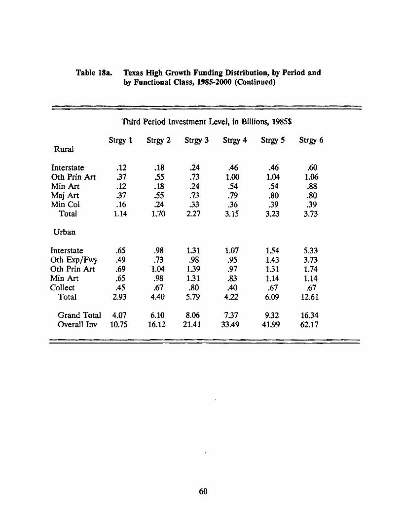
Table 18a. Texas High Growth Funding Distribution, by Period and by Functional Class, 1985-2000 (Continued)

Third Period Investment Level, in Billions, 1985$

Strgy 1 Strgy 2 Strgy 3 Strgy 4 Strgy 5 Strgy 6 Rural

Interstate .12 .18 .24 .46 .46 .60 0th Prin Art .37 .55 .73 1.00 1.04 1.06 Min Art .12 .18 .24 .54 .54 .88 Maj Art .37 .55 .73 .79 .80 .80 Min Col .16 .24 .33 .36 .39 .39

Total 1.14 1.70 2.27 3.15 3.23 3.73

Urban

Interstate .65 .98 1.31 1.07 1.54 5.33 0th Exp/Fwy .49 .73 .98 .95 1.43 3.73 0th Prin Art .69 1.04 1.39 .97 1.31 1.74 Min Art .65 .98 1.31 .83 1.14 1.14 Collect .45 .67 .80 .40 .67 .67

Total 2.93 4.40 5.79 4.22 6.09 12.61

Grand Total 4.07 6.10 8.06 7.37 9.32 16.34 Overall Inv 10.75 16.12 21.41 33.49 41.99 62.17

60

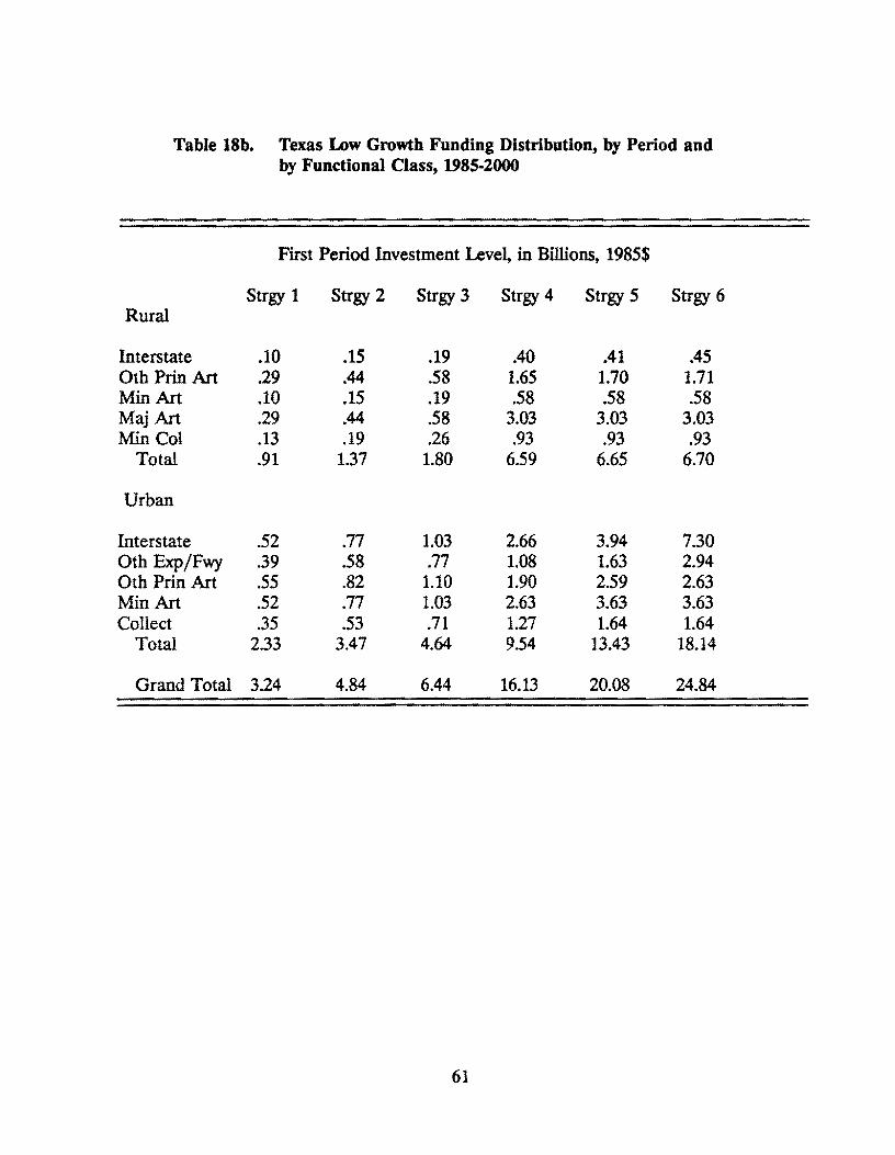
Table 18b. Texas Low Growth Funding Distribution, by Period and by Functional Class, 1985-2000

First Period Investment Level, in Billions, 1985$

Strgy 1 Strgy 2 Strgy 3 Strgy 4 Strgy S Strgy 6 Rural

Interstate .10 .15 .19 .40 .41 .45 0th Prin Art .29 .44 .58 1.65 1.70 1.71 Min Art .10 .15 .19 .58 .58 .58 Maj Art .29 .44 .58 3.03 3.03 3.03 Min Col .13 .19 .26 .93 .93 .93

Total .91 1.37 1.80 6.59 6.65 6.70

Urban

Interstate .52 .77 1.03 2.66 3.94 7.30 0th Exp/Fwy .39 .58 .77 1.08 1.63 2.94 0th Prin Art .55 .82 1.10 1.90 2.59 2.63 Min Art .52 .77 1.03 2.63 3.63 3.63 Collect .35 .53 .71 1.27 1.64 1.64

Total 2.33 3.47 4.64 9.54 13.43 18.14

Grand Total 3.24 4.84 6.44 16.13 20.08 24.84

61

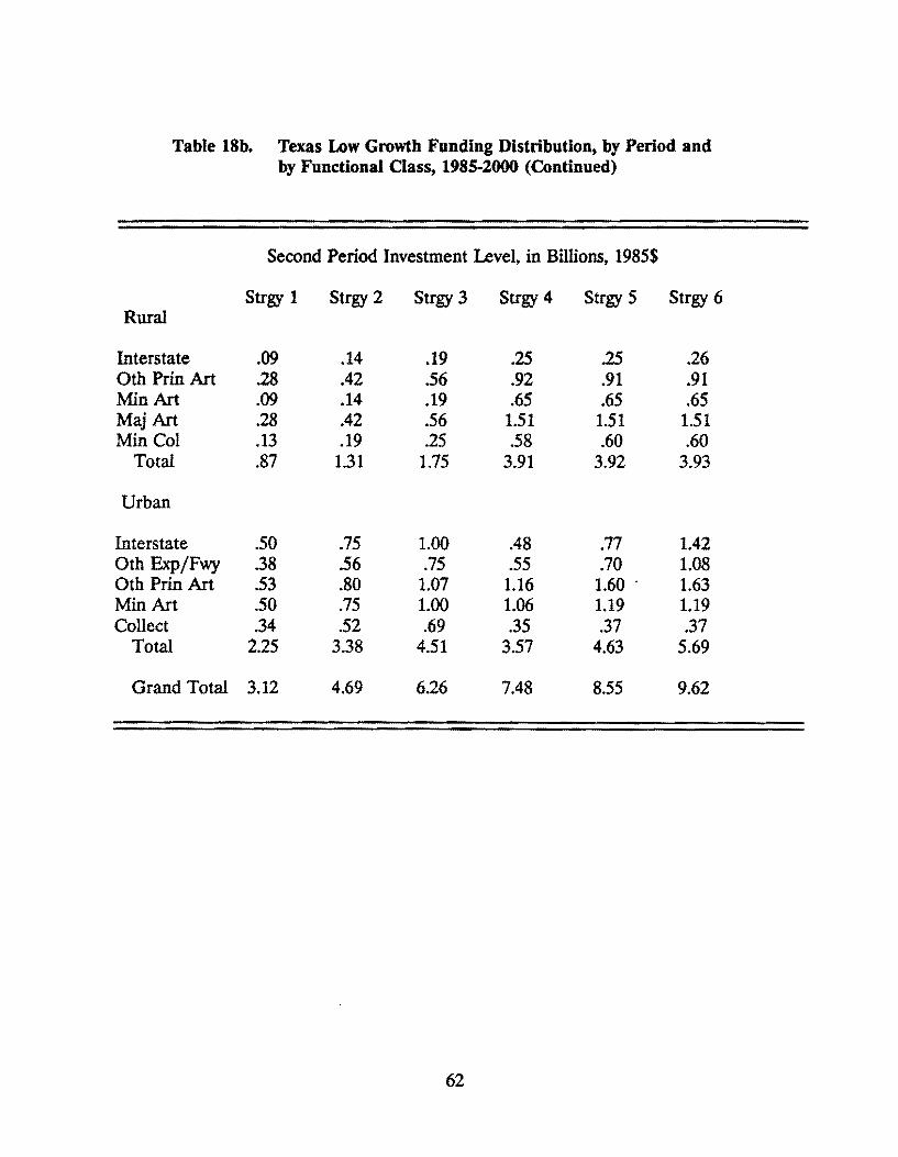
Table 18b. Texas Low Growth Funding Distribution, by Period and by Functional Class, 1985-2000 (Continued)

Second Period Investment Level, in Billions, 1985$

Strgy 1 Strgy 2 Strgy 3 Strgy 4 Strgy 5 Strgy 6 Rural

Interstate .09 .14 .19 .25 .25 .26 0th Prin Art .28 .42 .56 .92 .91 .91 Min Art .09 .14 .19 .65 .65 .65 Maj Art .28 .42 .56 1.51 1.51 1.51 Min Col .13 .19 .25 .58 .60 .60

Total .87 1.31 1.75 3.91 3.92 3.93

Urban

Interstate .50 .75 1.00 .48 .77 1.42 0th Exp/Fwy 38 .56 .75 .55 .70 1.08 0th Prin Art .53 .80 1.07 1.16 1.60 . 1.63 Min Art .50 .75 1.00 1.06 1.19 1.19 Collect .34 .52 .69 .35 .37 .37

Total 2.25 3.38 4.51 3.57 4.63 5.69

Grand Total 3.12 4.69 6.26 7.48 8.55 9.62

62

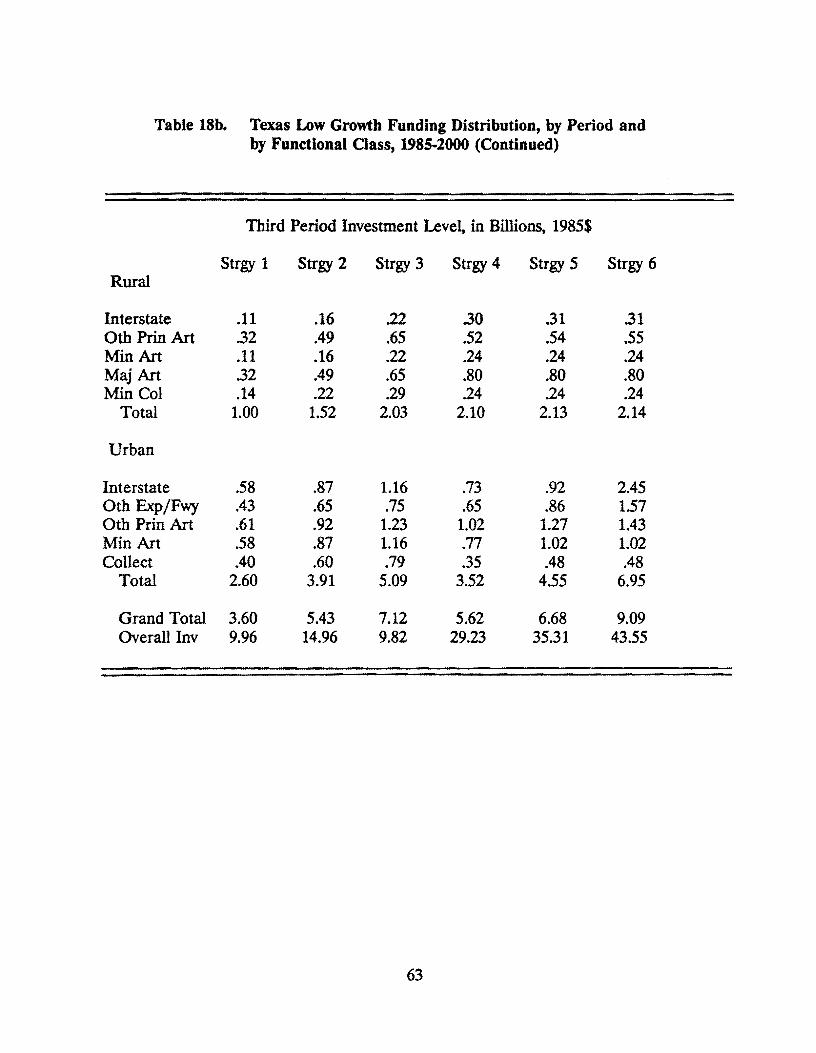
Table 18b. Texas Low Growth Funding Distribution, by Period and by Functional Class, 1985-2000 (Continued)

Third Period Investment Level. in Billions, 1985$

Strgy 1 Strgy 2 Strgy 3 Strgy 4 Strgy 5 Strgy 6 Rural

Interstate .11 .16 .22 .30 .31 .31 0th Prin Art .32 .49 .65 .52 .54 .55 Min Art .11 .16 .22 .24 .24 .24 Maj Art .32 .49 .65 .80 .80 .80 Min Col .14 .22 .29 .24 .24 .24

Total 1.00 1.52 2.03 2.10 2.13 2.14

Urban

Interstate .58 .87 1.16 .73 .92 2.45 0th Exp/Fwy .43 .65 .75 .65 .86 1.57 0th Prin Art .61 .92 1.23 1.02 1.27 1.43 Min Art .58 .87 1.16 .77 1.02 1.02 Collect .40 .60 .79 .35 .48 .48

Total 2.60 3.91 5.09 3.52 4.55 6.95

Grand Total 3.60 5.43 7.12 5.62 6.68 9.09 Overall Inv 9.96 14.96 9.82 29.23 35.31 43.55

63

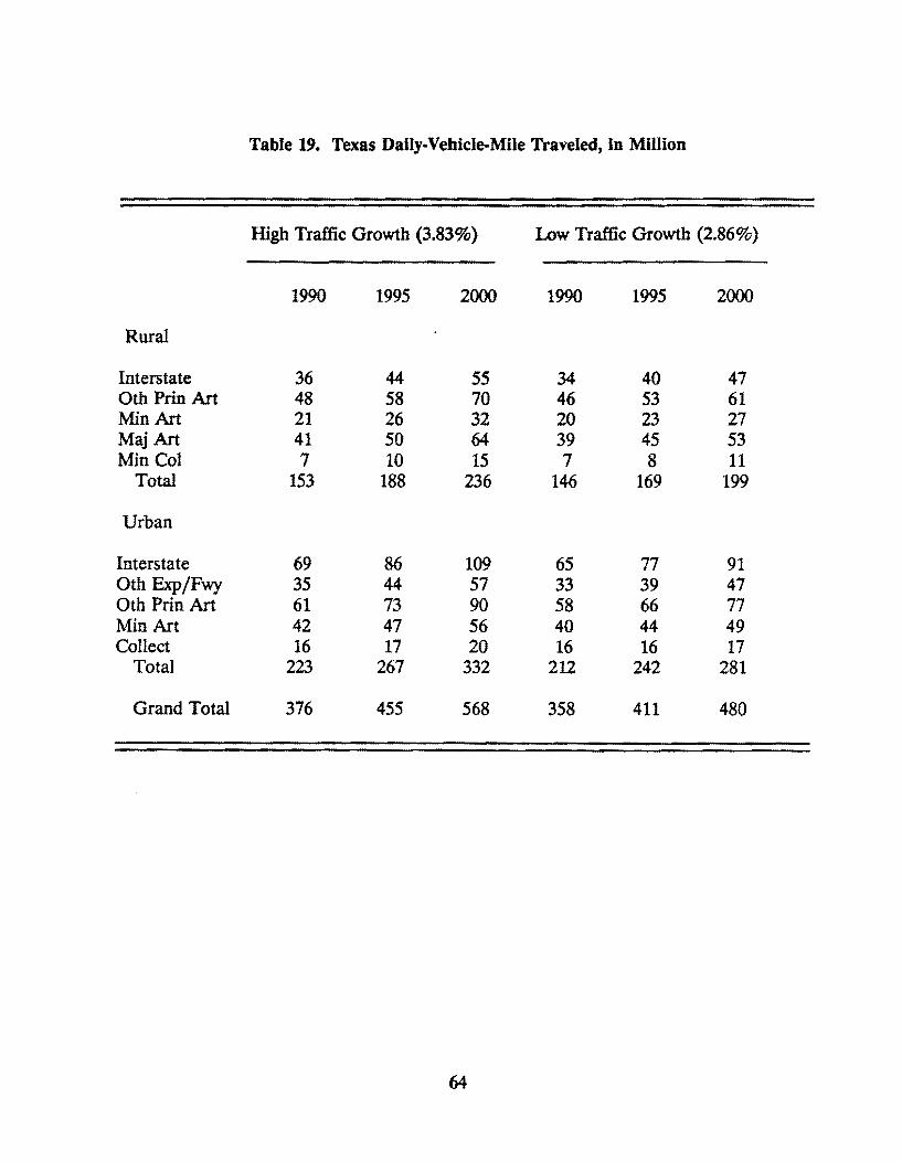
Table 19. Texas Daily-Vehicle-Mile Traveled, in Million

High Traffic Growth (3.83%) 1.Dw Traffic Growth (2.86%)

1990 1995 2000 1990 1995 2000

Rural

Interstate 36 44 55 34 40 47 0th Prin Art 48 58 70 46 53 61 Min Art 21 26 32 20 23 27 Maj Art 41 50 64 39 45 53 Min Col 7 10 15 7 8 11

Total 153 188 236 146 169 199

Urban

Interstate 69 86 109 65 77 91 0th Exp/Fwy 35 44 57 33 39 47 0th Prin Art 61 73 90 58 66 77 Min Art 42 47 56 40 44 49 Collect 16 17 20 16 16 17

Total 223 267 332 212 242 281

Grand Total 376 455 568 358 411 480

64

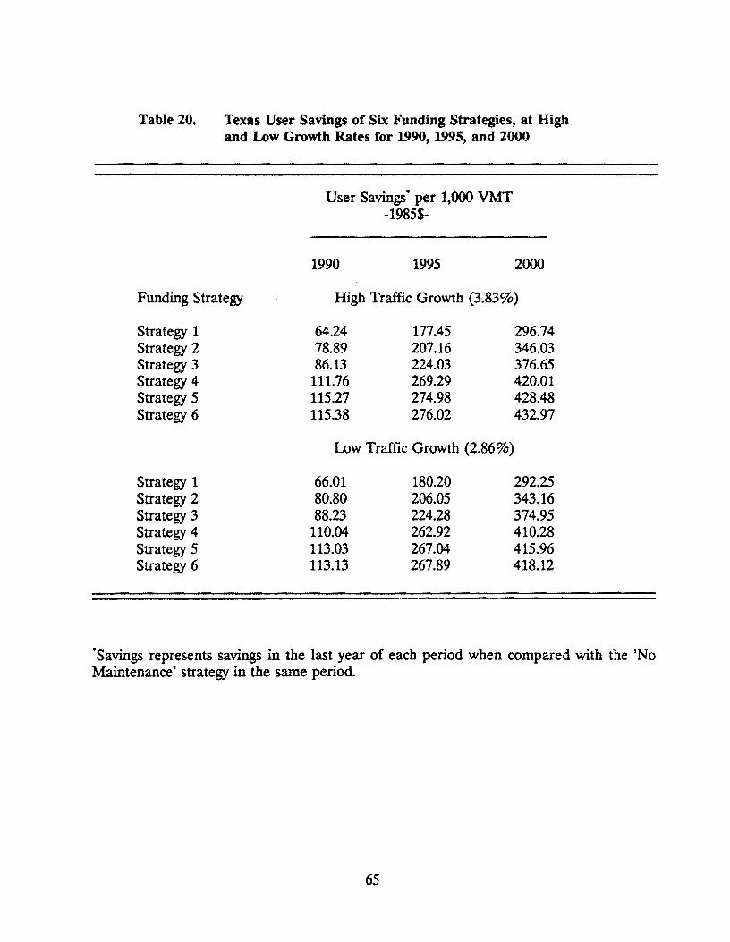
Table 20. Texas User Savings or Six Funding Strategies, at High and Low Growth Rates for 1990, 1995, and 2000

Funding Strategy

Strategy 1 Strategy 2 Strategy 3 Strategy 4 Strategy 5 Strategy 6

Strategy 1 Strategy 2 Strategy 3 Strategy 4 Strategy 5 Strategy 6

User Savings· per 1,000 VMT -1985$-

1990 1995 2000

High Traffic Growth (3.83%)

64.24 177.45 296.74 78.89 207.16 346.03 86.13 224.03 376.65

111.76 269.29 420.01 115.27 274.98 428.48 115.38 276.02 432.97

Low Traffic Growth (2.86%)

66.01 180.20 292.25 80.80 206.05 343.16 88.23 224.28 374.95

110.04 262.92 410.28 113.03 267.04 415.96 113.13 267.89 418.12

·savings represents savings in the last year of each period when compared with the 'No Maintenance' strategy in the same period.

65

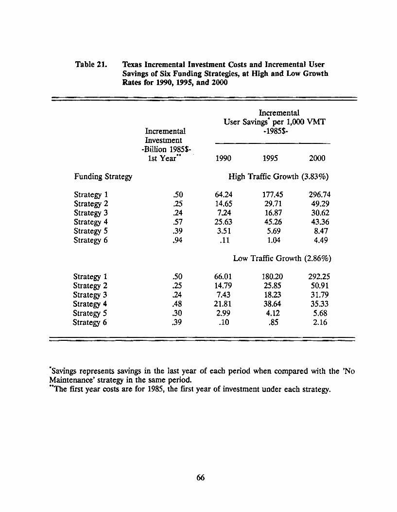
Table 21. Texas Incremental Investment Costs and Incremental User Savings or Six Funding Strategies, at High and 1..-0w Growth Rates ror 1990, 1995, and 2000

Incremental User Savings• per 1,000 VMT

Incremental -1985$-Investment

-Billion 1985$-1st Year

.. 1990 1995 2000

Funding Strategy High Traffic Growth (3.83%)

Strategy 1 .50 64.24 177.45 296.74 Strategy 2 .25 14.65 29.71 49.29 Strategy 3 .24 7.24 16.87 30.62 Strategy 4 .57 25.63 45.26 43.36 Strategy 5 .39 3.51 5.69 8.47 Strategy 6 .94 .11 1.04 4.49

Low Traffic Growth (2.86%)

Strategy 1 .50 66.01 180.20 292.25 Strategy 2 .25 14.79 25.85 50.91 Strategy 3 .24 7.43 18.23 31.79 Strategy 4 .48 21.81 38.64 35.33 Strategy 5 .30 2.99 4.12 5.68 Strategy 6 .39 .10 .85 2.16

·savings represents savings in the last year of each period when compared with the 'No Maintenance' strategy in the same period • .. The first year costs are for 1985, the first year of investment under each strategy.

66

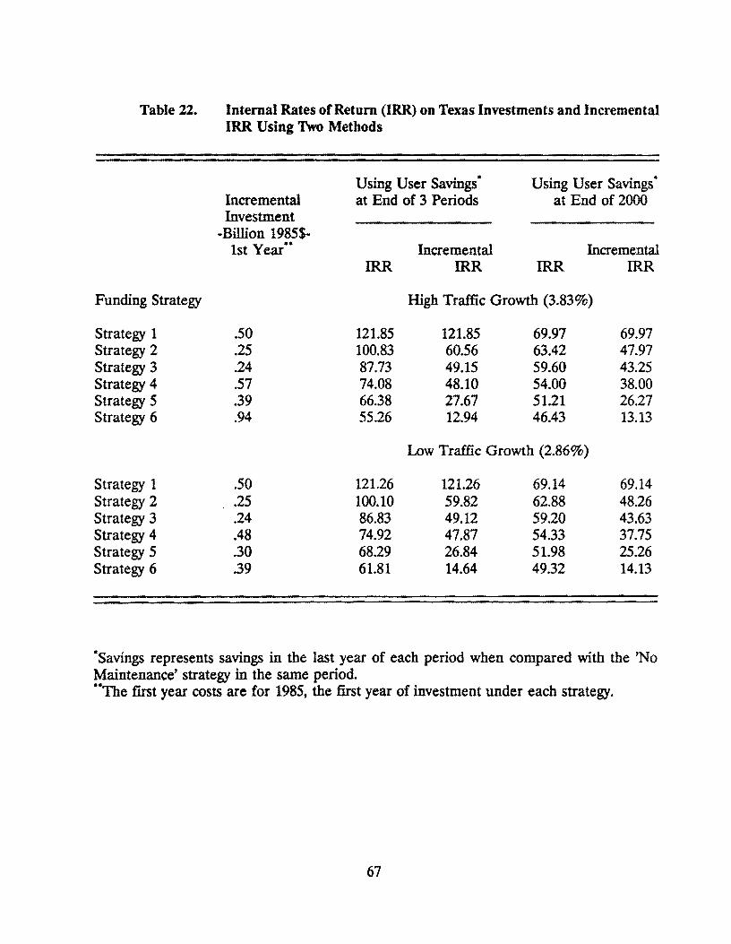
Table 22.

Funding Strategy

Strategy 1 Strategy 2 Strategy 3 Strategy 4 Strategy 5 Strategy 6

Strategy 1 Strategy 2 Strategy 3 Strategy 4 Strategy 5 Strategy 6

Internal Rates of Return (IRR) on Texas Investments and Incremental IRR Using Two Methods

Using User Savings • Using User Savings .

Incremental at End of 3 Periods at End of 2000 Investment

-Billion 1985$-1st Year •• Incremental Incremental

IRR IRR IRR IRR

High Traffic Growth (3.83%)

.50 121.85 121.85 69.97 69.97

.25 100.83 60.56 63.42 47.97

.24 87.73 49.15 59.60 43.25

.57 74.08 48.10 54.00 38.00

.39 66.38 27.67 51.21 26.27

.94 55.26 12.94 46.43 13.13

Low Traffic Growth (2.86%)

.50 121.26 121.26 69.14 69.14

.25 100.10 59.82 62.88 48.26

.24 86.83 49.12 59.20 43.63

.48 74.92 47.87 54.33 37.75

.30 68.29 26.84 51.98 25.26

.39 61.81 14.64 49.32 14.13

·savings represents savings in the last year of each period when compared with the 'No Maintenance' strategy in the same period . .. The first year costs are for 1985, the first year of investment under each strategy.

67

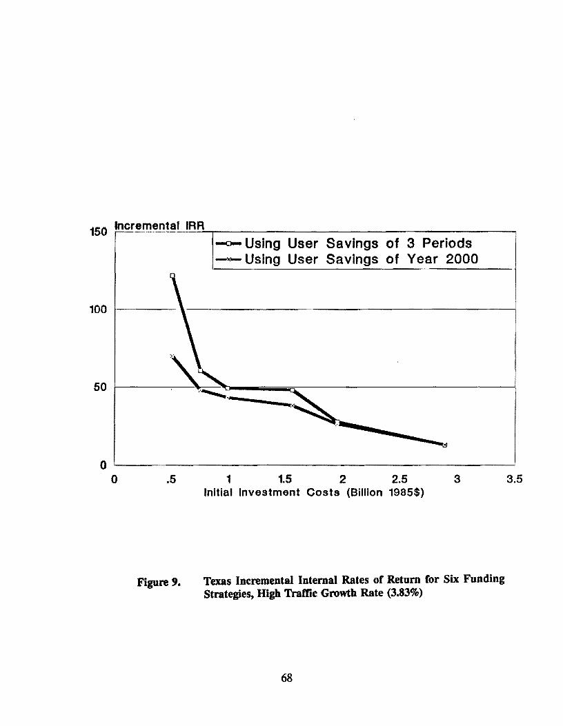
150 Incremental IRA

-c:::i- Using User Savings of 3 Periods -x- Using User Savings of Year 2000

0 '--~~~~~~~~~~~~~~~~~~~~~~~~

0 .5

Figure 9.

1 1.5 2 2.5 3 Initial Investment Costs (Billion 1985$}

Texas Incremental Internal Rates of Return for Six Funding Strategies, High Trame Growth Rate (3.83%)

68

3.5

150 Incremental IRR

0 0

--o- Using User Savings of 3 Periods -- Using User Savings of Year 2000

.5 1 1.5 2 2.5 Initial Investment Costs (Billion 1985$)

Figure 10. Texas Incremental Internal Rates of Return for Six Funding Strategies, Low Trame Growth Rate (2.86%)

69

high and low growth rates are unexpectedly high, as shown in Table 22, especially compared to the national results. While Strategy 7 for the United States (unconstrained, no lane restrictions, full needs) yields a negative incremental internal rate of return of -16 percent a similar strategy for Texas (Texas Strategy 6) still gives a high return of 13 to 14 percent, depending on the growth rate used. A major cause for the higher rates of return in Texas are the high returns on the urban Interstates and other freeway/ expressways categories in the unconstrained full needs scenario. Because of the widening feasibility under the unconstrained definition, with an unUmited budget, these two categories can be widened to reduce congestion and decrease user costs. Among the 148 sections of urban interstate highways, there were 21 sections which were widened to the maximum 12 lanes in the constrained scenario while 80 sections were widened in the unconstrained scenario.

In the unconstrained full needs scenario (Strategy 6), when the number of lanes is assumed to be unlimited, some sections were widened to as many as 31 lanes, and many were widened to 22 and 26 lanes. These results indicate that additional lanes probably will be needed to accommodate expected future traffic growth in these traffic corridors. Compared to the nation, Texas is predicted to have annual traffic growth rates of 3.14 percent and 3.10 percent for the urban Interstate and other freeway/expressway categories, respectively, while 2.07 percent and 1.88 percent growth rates are predicted nationally for the corresponding functional classes. At the last increment of expenditure studied, at funding of unconstrained full needs, highway investment in Texas is estimated to give a marginal rate of return of 13 to 14 percent, as shown in Table 22.

70

REFERENCES

1. American Association of State Highway and Transportation Officials, Keepina America Movina. The Bottom Line: A Sum.mazy of Surface Transportation Investment Requirements. 1988-2020. Washington, D.C., September, 1988.

2. Federal Highway Administration, The Future National Hiahway Pro~am: 1991 and Beyond. Workini Paper No. 13. Highway Performance and Investment Analysis, Washington, D.C., December, 1987.

3. National Council on Public Works Improvement, Fraiile Foundations: A Report on America's Public Works, Final Report to the President and Congress, U.S. Government Printing Office, February, 1988.

4. Congressional Budget Office, New Directions for the Nation's Public Works, U.S. Government Printing Office, September, 1988.

5. Transportation Research Board, National Research Council, A Look Ahead: Year 2020, Special Report 220, Washington, D.C., Transportation Research Board, 1988.

6. Federal Highway Administration, The Status of the Nation's Highways: Conditions and Performance, Report of the Secretary of Transportation to the United States Congress, pursuant to Section 307( e) of Title 23, United States Code, June, 1987, Washington, D.C., U.S. Government Printing Office, June, 1987. (This is the ninth in a series of Biennial reports to Congress pursuant to Section 307 of Title 23, United States Code.)

7. Pisarski, Alan E., The Nation's Public Works: A Report on Highways. Streets. Roads. and Bridges, Background paper prepared for the National Council on Public Works Improvement, May, 1987.

8. Aschauer, David A, "Rx for Productivity: Build Infrastructure," Chicago Fed Letter, Chicago, The Federal Reserve Bank of Chicago, Number 13, September, 1988.

9. "America is Buckling and Leaking," New.York Times, June 24, 1988.

10. Aschauer, David A, "Is Public Expenditure Productive?," Federal Reserve Bank of Chicago, 1989.

11. Senate Hearings, Subcommittee on Water Resources, Transportation, and Infrastructure, October 21, 1987. Also October 6, 1987. Also November 4, 1987.

12. Office of Management and Budget, Supplement to Special Analysis D, May, 1988.

71

13. Congressional Budget Office, U.S. Congress, Federal Policies for Infrastructure Management, June, U.S. Government Printing Office, 1986.

14. Association of General Contractors, America's Infrastructure, 1985.

15. Kaplan, Marshall, Hard Choices. A Report on the Increasina Gap Between America's Infrastructure Needs and Our Ability to Pay for Them: A Study. February, Washington, D.C., U.S. Government Printing Office, 1984.

16. National Highway Traffic Safety Administration (NHTSA), The Economic Cost to Society of Motor vehicle Accidents, Washington, D.C., 1983.

17. EXP Associates, ''Time Values per Vehicle Hour for Seven Vehicle Classes," March 1983.

18. American Association of State Highway and Transportation Officials, Keeping America Moving: Highway Needs. Structural Issues and Highway Operations, Report of the Transportation 2020 Highway Technical Advisory Committee {HTAC), Appendix 1 to The Bottom Line, Washington, D.C., September, 1988.

19. American Association of State Highway and Transportation Officials, Keeping America Moving: Public Transportation Needs, Report of the Transportation 2020 Modal Technical Advisory Committee (MT AC), Appendix 2 to The Bottom Line, Washington, D.C., September, 1988.

20. American Association of State Highway and Transportation Officials, Keeping America Moving: Modal Interlink Needs for Air. Water and Rail, Report of the Transportation 2020 Modal Technical Advisory Committee (MTAC), Washington, D.C., September, 1988.

21. Highway Users Federation, Beyond the Interstate: A Look at the Factors that Will Influence American Highway Mobility in the 1990's and into the 21st Century, Washington, D.C., no date (ca. 1988).

22. Highway Users Federation, Transportation Issues 1987, Washington, D.C., 1987.

23. Federal Highway Administration, Feasibility of a National Weight-Distance Tax, Forthcoming in CBO study.

24. Congressional Budget Office, U.S. Congress, federal Policies for Infrastructure Management, June, 1986.

25. Transportation Research Board, Designing Safer Roads: Practices for Resurfacing.

72

Restoration, and Rehabilitation. Special Report 214, Washington, D.C., Transportation Research Board, 1987.

26. Federal Highway Administration, Interstate Gap Study, Report of the Secretary of Transportation to the United States Congress, 1977.

27. House Banking and Currency Committee, The Urban Mass Transportation Act of .12.M., Report No. 204 to Accompany H.R. 3881, April 9, 1963.

28. George W. Hilton, The Urban Mass Transportation Assistance PrOifa.tl1 American Enterprise Institute Evaluation Studies, No. 17, Washington, D.C., June, 1974.

29. Senate Hearings, Subcommittee on Water Resources, Transportation, and Infrastructure, October 21, 1987. Also October 6, 1987. Also November 4, 1987.

30. Office of Management and Budget, Supplement to Special Analysis B, May, 1988.

31. Congressional Budget Office, U.S. Congress, Federal Policies for Infrastructure Manaiement, Washington, D.C., June, 1986.

32. Association of General Contractors, America's Infrastructure. 1984?.

33. Joint Economic Committee, U.S. Congress, Hard Choices, Washington, D.C., U.S. Government Printing Office, February, 1984.

34. Tresch, Richard, Public Finance: A Normative Theoty, Plano, Texas: Business Publications, Inc., 1981.

35. Apogee Research, Inc., Infrastructure Issues Problems and General Solutions, Report prepared for the National Council on Public Works Improvement, October, 1986.

36. Apogee Research, Inc., The Nation's Public Works: A Report on Airports and Airways. Background paper prepared for the National Council on Public Works Improvement, May, 1987.

37. Kirby, Ronald F., and Arlee T. Reno, The Nation's Public Works: A Report on Mass Transit, Background paper prepared for the National Council on Public Works Improvement, May, 1987.

38. Revis, Joseph S. and Curtis Tarnoff, The Nation's Public Works: A Report on Intermodal Transportation, Background paper prepared for the National Council on Public Works Improvement, May, 1987.

39. National Council on Public Works Improvement, The Nation's Public Works:

73

Definina the Issues, Washington, D.C., 1986.

40. Peterson, George E., Ted Miller, Nancy Humphrey, and Christopher Walker, Infrastructure Needs Studies: A Critiqye, The Urban Institute, July, 1986.

41. Federal Highway Administration, The Future National Hi~hway Proifam: 1991 and Beyond, Washington, D.C., 1987 and 1988. A series of working papers entitled:

No. 1 Changing Demographics and Economic Base No. 2 Trends and Forecasts of Highway Passenger Travel No. 3 Trends and Forecasts of Highway Freight Travel No. 4 Advancements in Highway Materials and Construction Technology No. 5 Advancements in Automobile Technology No. 6 Advancements in Truck Technology No. 7 Advancements in Vehicle and Traffic Control Technology No. 8 Advancements in Telecommunications and Computer Technology Affecting

Highway Travel No. 9 National Defense Highway Requirements No.10 Urban and Suburban Highway Congestion No.11 Intercity and Interstate Travel and Network Congestion No.12 Highway Requirements for Freight Movement No.13 Highway Performance and Investment Analysis No.14 Overall Highway System Requirements and Investment Levels No.15 Federal Role Determination Criteria No.16 Federal Highway Investment Program Structure No.17 Federal Mandates for Highway Operations and Safety No.18 State, Local, and Private Roles No.19 External Federal Policies

42. Apogee Research, Inc., The Uses and Misuses of Infrastructure Needs Surveys and Inventories, July, 1986.

43. Cucitti, Peggy and E. Sam Overman, The Assessment of Investment Needs: A Review of Current Estimates and Awroaches, Center for Public Private Sector Cooperation, Graduate School of Public Affairs, University of Colorado at Denver, July, 1986.

44. Hulten, Charles R. and George E. Peterson, 'The Public Capital Stock: Needs, Trends, and Performance," American Economic Review, May, 1984, pp. 166-173.

74