AGRICULTURAL ECONOMICS

ELSEVIER Agricultural Economics 15 (1996) 47-60

An application of cointegration theory in the estimation of the Almost Ideal Demand system for food consumption in Bulgaria

K.G. Balcombe a, J.R. Davis b,*

a Department of Agricultural Economics, Wye College, University of London, Kent, TN25 5AH, UK b CERT, Department of Economics, Heriot Watt Business School, Heriot Watt University, Edinburgh EH14 4AS, UK

Accepted 26 April 1996

Abstract

The Almost Ideal Demand system is applied to consumption in Bulgaria. It is argued that the conventional estimation of the Almost Ideal model should be done within the framework of contemporary time series methodology. In this paper, the canonical cointegrating regression procedure of Park is applied. It is argued that the results of the Almost Ideal Demand system that are presented are consistent with both theory and 'casual' observation of consumer behaviour in Bulgaria.

1. Introduction

The Almost Ideal Demand system (Deaton and Muellbauer, 1980a) is derived from the static theory of optimising household behaviour. Households are assumed to have fundamentally similar preferences and choose their optimal bundle of homogeneous goods at one point in time, given perfect informa­tion. The estimation of the Almost Ideal (AI) model to available time series data is the application of a static model (using a flexible but nevertheless restric­tive functional form) to what must be assumed to be an evolution of the collective, dynamic, optimising behaviour of non-homogeneous households, making decisions based on partial information.

The estimation of the AI model and other models of a similar 'duality' in nature (Antle and Capalbo, 1988), using time series data, has been increasingly popular. Considerable energy has been devoted to

' Corresponding author.

the analysis of the appropriateness of the functional forms and their ability to approximate the behaviour of 'rational' agents (Christensen et al., 1975; Lau, 1986) and to allow aggregation across consumer groups. The theory of estimation and inference has, for the most part, been confined to the issue of whether to use maximum likelihood (ML) in the estimation of the AI model or to use the Seemingly Unrelated Regression (SUR) method applied to lin­ear approximations of the AI model. In either case the underlying 'static' assumptions such as homo­geneity and symmetry (see Section 5) have been tested using the classical rules of inference under the implicit assumption that the regressors are stationary and ergodic processes (Hamilton, 1994, pp. 45-46).

Since the publication of Deaton and Muellbauer's paper (Deaton and Muellbauer, 1980a), there has been considerable advancement in the theory con­cerning the estimation and inference in systems that have stochastic processes which are clearly not of the stationary and ergodic type. The work of many authors, notably in the early 1980s, such as Granger

0169-5150/96/$15.00 Copyright© 1996 Elsevier Science B.V. All rights reserved. Pll SO 169-5150(96)0 1190-5

48 K.G. Balcombe, J.R. Davis/ Agricultural Economics 15 ( 1996) 47-60

(1981), Granger and Weiss (1983), Phillips (1986, 1987), Engle and Granger (1987), did much to ad­vance time series analysis on two united fronts. The first front was the question of estimation and infer­ence with non-stationary variables, and the second was the methodological approach to modelling which was, in part, to view the use of static theory as the 'long run equilibrium' and to unite this with the concept of 'cointegration'. Subsequent work by writ­ers such as Stock and Watson (1988), Park and Phillips (1988, 1989), Johansen (1988), Phillips and Ouliaris (1990), Phillips and Hansen (1990), Saikko­nen (1991) and Park (1992) has catalogued and developed techniques for estimation and inference about long run equilibrium relationships between variables with unit roots at the zero frequency. The cointegration framework has become the new paradigm within time series econometrics (although not without its critics: Sims, 1988). However, much contemporary work using 'duality based' models (such as the AI system) continues to ignore these developments within time series analysis, with a few exceptions (Ogaki and Park, 1989; Clark and Young­blood, 1992).

Duality based models provide a guide to the selection of appropriate transformations of the data and a set of restrictions on the parameters of the system. Integration and cointegration theory provides the avenue through which static theory may be ap­plied in the empirical context. It also provides the theoretical basis and framework, when applied to duality based models, for the testing of the static rationality propositions of utility maximisation or profit maximisation as 'long run' conditions. Cointe­gration is as much about the relevant exogeneity conditions needed for valid estimation and inference, as about whether the regression is 'spurious' (in the sense of Granger and Newbold, 1986, p. 205). In this paper an equally important role is given to the consideration of the underlying data-generating pro­cess and structural model suggested by the AI frame­work. It is also stressed that what is at issue here is whether the innovations in the errors of the demand equations are independent of the price innovations: a condition that is unlikely to be fulfilled.

In this paper the canonical cointegrating regres­sion (CCR; Park, 1992) procedure is employed in estimating the almost ideal demand system for food

consumption in Bulgaria. The relevance of this pro­cedure along with other issues is discussed in Sec­tion 2. In Section 3 Section 4 the Bulgarian economy is overviewed along with the data used in estimation. In Section 5 the AI model is presented in its theoreti­cal form, and in Section 6 the consequences of estimating the linear approximation of the AI model is discussed. In Section 7 Section 8 the empirical results are presented and discussed. Where it is necessary, the use of the techniques is supported with Monte Carlo evidence in Appendix B. An outline of the estimation procedure is presented in Appendix A.

2. Issues in estimation

In this section several issues are emphasised. First, the AI model is interpreted as a set of long run equilibrium equations. In all likelihood the specifica­tion of this static system neglects the existence of lag structures. Consequently, the error structure in AI models would be serially correlated, and possibly heteroscedastic as well. Second, the existence of a set of supply equations almost certainly implies that the error terms in the AI model are not independent of the regressors. Third, the data used in estimating the models cannot a priori be assumed to be station­ary.

The utility in claiming that the equations represent equilibrium relationships is that, providing the data have trends, the estimated parameter values (using Ordinary Least Squares (OLS), SUR or ML) con­verge (superconsistently) to their long run population values, if the error structures obey conditions that are weaker than stationarity (Phillips, 1987). The signifi­cance of this result is that the existence of depen­dence between the errors in the equations and the innovations in the regressors does not cause inconsis­tency of the parameter estimates. On the other hand, the application of Wald, Likelihood Ratio (LR) or Lagrangian Multiplier (LM) (Godfrey, 1988, pp. 1-39) tests is invalidated in circumstances where the errors are not strictly exogenous to the regressors (Park, 1992, p. 129).

It is wise to be circumspect in accepting claims that the conventional estimation techniques will al­ways produce consistent estimates of structural pa­rameters in a cointegrating regression. There may

K.G. Balcombe, J.R. Davis/ Agricultural Economics /5 ( 1996) 47-60 49

exist up to n - 1 cointegrating relationships between n variables with a unit root and the zero frequency (Johansen, 1988). The structural relationship may I:~present one such cointegrating vector, but the esti­mated relationship may be some combination· of these cointegrating relationships. Alternatively, there may be omitted variables that are cointegrated with Ulose in the model. Furthermore, the data may have unit roots at non-zero (seasonal) frequencies and it is possible that there are several cointegrating relation­ships between just two variables at their seasonal frequencies (Engle et al., 1993). If the seasonality is deterministic (in the manner of Eq. (2.6) in Section 5) or the cointegrating vectors are the same at all frequencies, then the estimates remain consistent.

The primary aim in this paper is to examine the consumption behaviour of Bulgarian households. The p11per ignores the possibility that the data may have unit . roots at non-zero frequencies. Seasonality is treated· in a deterministic manner. The dynamics of ;onsumption behaviour (error correction models, etc.) are not modelled and the possibility that prices are themselves cointegrated is not considered. The focus is upon the AI model as a guide to the specification of a set of long run equilibrium relations between ',!ariables. that have univariate behaviour consistent with.the unit root hypothesis. A major concern is that hypothesis tests are constructed in a valid way. The CCR.procedure is among the range of options now available Jo estimate these cointegrating relations while allowing for the fact that the error terms may not be strictly exogenous to the regressors in the model. In previous studies employing 'duality based' models, it has been common to reject assumptions that are intrinsic to the construction of these models (see Section 5, Eqs. (1.5), (1.6) and (1.7)). However, tl)e . auxiliary hypotheses employed in conducting inference are, arguably, less believable than the main hypotheses which they purport to test. '! In addition to the issues raised above, the merits

of the linear approximation of the AI system is c.onsidered. As can be examined in Section 5, the AI model is not linear. Deaton and Muellbauer ( 1980a) suggested that an approximation of the price index known as Stone's index could serve as a useful simplification. Alternatively, the CCR procedure could be adapted by using an iterative estimation procedure and then employing the CCR procedure at

the last stage of estimation. Of concern is whether the linear approximation works, and whether the univariate behaviour of the data has anything to do with its performance. Previous papers have tended to focus on what happens to ·the parameter estimates (Pashardes, 1992) but have not considered its impact on inference.

Finally, estimation has been done over a period of rapid structural change in the Bulgarian economy: The use of pretransformation price data may intro­duce additional bias in the results, to the extent that the regulated prices of goods on the market deviate from the true cost of purchase to the consumer 1•

However, providing the wedge between observed prices and 'true' prices is of a stationary order then there should be efficiency gains in the use of this data, which outways the bias that is introduced. Testing for structural stability within the cointegra­tion framework is a complicated issue (Hansen, 1992; Zivot and Andrews, 1992). The issue is further com­plicated by the fact that we have relatively small sample sizes over which we could estimate separate long run variance-covariance matrices so as to per­form modified Chow tests or pursue the type of recursive tests discussed in the papers directly above. Tests for structural change are not presented in this paper, and a dummy variable is placed at the point of liberalisation. The short sample size and the struc­tural change are undeniably problematic. The inclu­sion of transition dummy may not fully account for the structural change. Moreover, the methods being used rely on asymptotic results. In defence. of the work, two points are noted: first, a change in the distribution of the conditioning variables (prices), does not necessarily negate the possibility of having stable structural parameters of a system (Engle et al., 1983). Second, the existence of structural break will tend to cause a failure to reject the· hypothesis of non-cointegration.

3. An overview of the Bulgarian economy and restructuring

Macroeconomic imbalances in Bulgaria are the product of a tightly controlled system of central

1 Which would also include the costs ~f queuing, etc.

50 K.G.·Balcombe, J.R. Davis/ Agricultural Economics 15 (1996) 47-60

planning. This remained intact until 1989. The sys­tem redirected economic growth towards heavy in­dustry and away from areas of comparative advan­tage like agriculture. Bulgaria became increasingly dependent upon its specialisation within the Come­con (CMEA) area, and neglected efficiency issues in the allocation of resources. For almost 40 years this strategy was able to generate a growth rate of 4-5% per annum. However, by the 1980s the limits of this strategy were reached progressively as economic de­terioration set in. This deterioration was masked by

· official statistics which overstated growth and living standards during the period. In 1989 for the first time in a decade, real net material product officially de­clined (National Statistics Institute, 1990).

The economic and political transformation in Bul­garia commenced in November 1989. Macroeco­nomic reform, including substantial price liberalisa­tion, commenced in January 1991. The short run effect of internal convertibility of the Bulgarian lev was a devaluation to one-twentieth of the prereform value. Following price liberalisation, the rate of in­flation as measured by the consumer price index (taken as 100% on I May 1990) was 50.6% by the end of 1990. It was 473.7% for the whole of 1991, 79.5% in 1992 2 and 63.9% in 1993. Interest rates jumped to 60% in nominal terms, while in real terms they continued to be negative.

These conditions, coupled with the uncertainties for production created by the cessation of central planning and the disappearance of traditional export markets, brought about deep recession. The negative economic growth of -9.1% in 1990 accelerated to -17% in 1991, and unemployment rose from 1.6% to 11.7%. respectively (OECD, 1992). Preliminary data for 1993 shows a negative growth of - 3:5% in real terms and unemployment approaching 16% (Bulgarian National Bank, 1993). The net effect was that, whilst nominal incomes grew five-fold from 1990 to 1992, real incomes for the same period fell by about two-thirds.

The price liberalisation of 1991 was regarded as a prerequisite to an improvement in the range and

2 This is the consumer price index published by the National Statistics Institute, Sofia. According to the Bulgarian National Bank, inflation in 1992 was 90%.

quality of goods and services characteristic of a market economy, because prices had been main~ tained at artificially low levels 3• Some of the ex;­pected benefits of liberalisation appeared quite quickly. In particular, queues for basic foodstuffs soon disappeared. This was partly as a result o,f improvements in domestic availability, helped not by improvements in production and distribution, but by the loss of export markets particularly in the former Soviet Union. It was also assisted by a contraction in consumption of many foods.

4. The data for the AI demand system

The model is estimated using monthly household budget survey data, monthly consumption data in kilogram per capita, expenditure and unit value data calculated from a National Statistical Institute (NSI) of Bulgaria survey (1992). The period over which estimation took place was from January 1989 to December 1992. inclusive. The main source of infor.~ mation used in this model is based on the household budget survey because it provides comparability over several years in fine commodity detail and at a low level of aggregation. During 1992 some changes were introduced in the grouping of products and services for which expenditures were recorded. These changes were not judged to make serious difficulty . for analysis.

The household budget surveys are based on a random sample of households covering all regions in the country and all social groups. The number of households covered in the survey varies annually, averaging about 2500 households and 7700 respon­dents. Since 1992 the NSI of Bulgaria has made ail attempt to cover new social groups which emerged during the postreform period (i.e. the self-employe~· and the unemployed). Reported maximum statistical errors in the survey are relatively small: 1.5% for income, and 2.8% for expenditures, including 2% for expenditure on food. In 1991 and 1992 the survey

3 Two systems of protection from the effects of food pric~ liberalisation are in operation: the projected price system, and th,e indexation of social benefits, wages and pensions to the price of food.

K.G. Balcombe, J.R. Davis/ Agricultural Economics 15 ( 1996) 47-60 51

covered 2508 households. The 1992 sample was based on the occupation of the head of a household and included 1252 pensioners and other economi­cally non-active persons, 1087 hired persons, 75 unemployed, 70 self-employed and 24 members of producer cooperatives.

The prices used in the model are undeflated unit values 4• These reflect the price per unit of consump­tion of a particular commodity. No prices per se are collected in the consumer budget survey. Unit values are calculated from survey information on expendi­tures and consumption.

The number of goods to be considered is limited to the commodities that are central to the average Bulgarian diet: bread, milk, cheese, meat; other foods including fats, sugar, vegetables, fruit and alcohol. Bread (white and Dobrudja), milk and yoghurt, cheese (white and yellow) and meat (all types) ac­counted for 42% of food expenditure in 1989 and 48% in 1992. Recognising that these products make up the major part of food consumption, they have been the principal products subject to price monitor­ing. The model has also used non-food expenditure data. This data includes: clothes and shoes, home appliances, culture, hygiene, communications and transport. The products analysed accounted for 62% of food expenditure and 43% of total expenditure.

5. Theoretical model

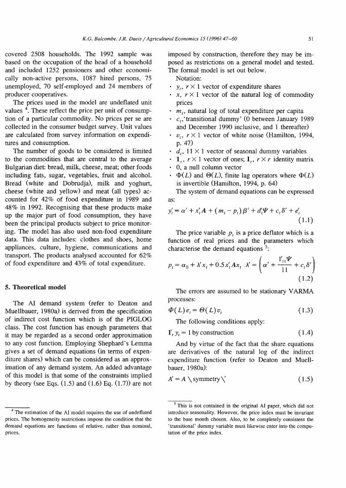
The AI demand system (refer to Deaton and Muellbauer, 1980a) is derived from the specification of indirect cost function which is of the PIGLOG class. The cost function has enough parameters that it may be regarded as a second order approximation to any cost function. Employing Shephard's Lemma gives a set of demand equations (in terms of expen­diture shares) which can be considered as an approx­imation of any demand system. An added advantage of this model is that some of the constraints implied by theory (see Eqs. (1.5) and (1.6) Eq. (1.7)) are not

4 The estimation of the AI model requires the use of undeflated prices. The homogeneity restrictions impose the condition that the demand equations are functions of relative, rather than nominal, prices.

imposed by construction, therefore they may be im­posed as restrictions on a general model and tested. The formal model is set out below.

Notation: Yt> r X 1 vector of expenditure shares x, r X 1 vector of the natural log of commodity prices m 1, natural log of total expenditure per capita c1,'transitional dummy' (0 between January 1989 and December 1990 inclusive, and 1 thereafter)

• v,. r X 1 vector of white noise (Hamilton, 1994, p. 47)

as:

d,. 11 X 1 vector of seasonal dummy variables lr, r X 1 vector of ones; Ir, r X r identity matrix 0, a null column vector cf>(L) and ®(L), finite lag operators where cf>(L) is invertible (Hamilton, 1994, p. 64) The system of demand equations can be expressed

y; =a'+ x;A + (m 1 - p,)/3' + d',P+ c1 8' + e; ( 1.1)

The price variable p 1 is a price deflator which is a function of real prices and the parameters which characterise the demand equations 5 :

+ ,, + 0 5 I A " = ~' + - 1- 1- + c "' ( I' p ) p 1 = a 0 llX1 • x, X 1 ll .... II ,u

( 1.2)

The errors are assumed to be stationary VARMA processes:

<P(L)e,= B(L)v,

The following conditions apply:

l'rY1 =I by construction

( 1.3)

( I.4)

And by virtue of the fact that the share equations are derivatives of the natural log of the indirect expenditure function (refer to Deaton and Muell­bauer, I980a):

A' = A \symmetry\' ( 1.5)

5 This is not contained in the original AI paper, which did not introduce seasonality. However, the price index must be invariant to the base month chosen. Also, to be completely consistent the 'transitional' dummy variable must likewise enter into the compu­tation of the price index.

52 K.G. Balcombe, J.R. Davis/ Agricultural Economics 15 ( 1996) 47-60

fr A= 0' \homogeneity\' and by 1.5 = A.lr = 0

( 1.6)

l'ra= 1 \additivity\' ( 1.7)

Hence it follows from the above conditions (Eqs. (1.4), (1.5), (1.6) and (1.7)) that:

fr/3=0', P.lr=O, frB=O' andl'r<P- 1(L)

.@( L) =0' ( 1.8)

The demand elasticities are (for derivation see Ray, 1980):

Uncompensated price gM ,1

=w(y1)-1(A-f3(A'+x'1A))-lr (2.0)

Expenditure YJ1 = w( g1)- 1 f3 + lr (2.1)

Compensated price gu,1 = gM,t + f3y; (2.2)

where w( y) is a square diagonal matrix with the share vector as its diagonal elements. The Hessian of the indirect cost function is:

(2.3)

An additional requirement of the model is that this Hessian matrix is semi-negative definite at all points in the data set. This cannot be imposed a priori using linear restrictions (Lau, 1978). The addi­tivity conditions imply that the variance-covariance matrix of the errors is singular. Therefore, any esti­mation technique which incorporates the inverse of covariance matrix (or a long run covariance matrix) must eliminate one of the equations. In the following one of the equations is eliminated and the notation is simplified in the following way:

y; = ( .Y; ,yr.J where y1 = ( r- 1) X 1 vector of shares

(2.4)

q;=(1,d~,c1 )

Y'=(yT, ... y1)

P' = ( PT, .. · P1)

M' = (mT, ... m 1)

E' = ( eT' .. . e I)

Z= (Q,X,M-P) K= (X,M-P)

The reduced version of Eq. (1.1) is written as

Y=ZTI +E (2.5)

where TI = (TI'1 ,TI'2 )' is partitioned conformably with Z = (Q,K). The stochastic component is represented as:

<Pk(L)(1-L)k1 =JL+Ed1 +l9k(L)u1 (2.6)

where <l>k(L) and ®k(L) are finite polynomial lag operators, <l>k(L) is invertable and u1 is a white noise vector. Furthermore, it is possible that past errors in the share equations are not strictly exoge­nous to the innovations in k 1• When it is considered that these are demand equations, it is likely that past disequilibrium (within the cointegration framework we interpret e1 to be disequilibrium) would impact on prices contemporaneously or through time. There­fore, the long run covariance matrix is defined as:

00

-00

and w; = ( e~ ,Llk~) 00

A= LT(i), F= T(O) +A i= I

(2.7)

(2.8)

The relevant partitioning of these matrices is:

nl2] J2 where fl II = ( r - 1) X ( r- 1) 21

(2.9)

and r, T(O) and A are partitioned in the same manner.

This is presented as part of the model so as to emphasise the fact that it is not, in general, justifi­able to assume that A 12 , A 21 or T(0) 12 are zero matrices. In the stationary world the main considera­tion is that T(0) 12 is zero. The application of a generalised least squares procedure accounting for any serial correlation in the error structure would (where T(0) 12 = 0) lead to consistent parameter esti­mates and asymptotically valid Wald tests. In the non stationary case, however, the fact that A 12 is not the null matrix would cause the W aid tests to be invalid. On the other hand, in the non-stationary case we no longer require T(0) 12 to be the null matrix in order to get the consistency of the parameter esti­mates. This is important because the estimation of the AI set of equations neglects the existence of a set of supply equations. Consequently, the simultaneous equation bias is eliminated asymptotically in the

K.G. Balcombe, J.R. Davis j Agricultural Economics 15 ( 1996) 47-60 53

non-stationary case, providing the system is cointe­grated and the set of cointegrating vectors is unique. The CCR procedure transforms the data so that the influence of the errors in equations on the innova­tions in the regressors is removed asymptotically. However, the CCR procedure is designed for a linear model. Clearly, the AI model presented above is non-linear in its parameters. How to adapt Park's procedure to the AI model is now considered.

6. Dealing with non-linearity

If the matrix P was observable then we could proceed according to the standard CCR procedure (see Appendix A). The non-linearity of the AI model may be avoided using Stone's approximation: - I Pr=YtXt (3.0)

This follows the suggestion of Deaton and Muell­bauer who demonstrate that the Stone's index (Stone, 1954) can have a close linear association with the index in Eq. (1.2). Alternatively, researchers have opted for maximum likelihood estimation. and in doing so neglected other issues such as serial correla­tion or the consideration of unit roots. Maximum likelihood can easily accommodate the specification of unit roots. However, the joint treatment of unit roots and serial correlation proves to be more diffi­cult (i.e. the case where A 12 =I= 0). There are, there­fore, considerable advantages in estimating Stone's

Table I Unit root tests

Variable Levels ADF: P = 2

Bread share -2.34 Milk share -1.67 Cheese share -2.09 Meat share -2.40 Other food share -3.50 Bread price -0.88 Milk price -0.84 Cheese price -0.83 Meat price -0.72 Other food price - 1.29 Non-food price -0.86 Real expenditure -2.59

Critical values: ' 10%, - 2.63; ' ' 5%, - 2.9. ADF, augmented Dickey-Fuller.

Levels Z1

0.35 -0.54

0.52 0.02

-0.10 -0.18 -0.04

1.68 2.14 1.25 1.22 6.61

approximation, if it works, since the methods sug­gested by Phillips and Hansen (1990) and Park (1992) would be applicable (since they are for linear mod­els).

This does not exhaust the options. Deaton and Muellbauer hint at the fact that an iterative approach could be taken where the Stone's index was used in the first instance, estimated by SUR, and then the index computed and used in a second stage of esti­mation and so on (Deaton and Muellbauer, 1980a, p. 321). The details of the iterative approach to the estimation of the full AI model are presented in Appendix A. Standard errors are computed (and W ald tests) in the last stage: treating the estimated price index as being a 'given' random variable. The iterative technique also allows the use of the CCR procededure at the last stage of estimation. The salient results of a Monte Carlo study are presented in Appendix B. In short, there are considerable dif­ferences between the AI system and the linear ap­proximation of the AI system when conducting infer­ence using standard or modified (see Appendix A) W ald tests. The technique is applied to the Bulgarian case in Section 8.

7. Univariate behaviour of the data-testing for unit roots

In this paper attention is restricted to the case of deterministic seasonality. Nevertheless, the issue of

First difference ADF: P = 2 First differenfe Z1

-4.3 ' ' -28.01 '. -4.3 ' ' -26.1 ' ' -3.37 ' ' -25.07 ' ' -4.09 '' -11.1'*

-3.79 ** -19.40'' -4.05 • ' -6.16 * * -3.34 ' ' -6.51 • ' -3.71 •• -7.24'' -3.39 •• -6.21 • ' -2.75 ' -6.43 ' ' -4.70 •• - 16.8 ' • -3.86 * ' -21.1 ''

54 K.G. Balcombe, J.R. Davis/ Agricultural Economics 15 ( 1996) 47-60

seasonality complicates the testing of unit roots. Engle et al. (1993), suggest that in testing for unit roots at the zero frequency is most easily achieved by smoothing the data (y) by using S(L)y1 = (1-L)- 1(1- U)y1 then conducting the standard aug­mented Dickey and Fuller (1979) tests. This proce­dure would be valid, in the case of stochastic or deterministic roots. The problem with this procedure that is has low power in small samples. Conse­quently, testing for unit roots will often result in the failure to reject unit roots in stationary series (espe­cially in the case of the monthly data). The same problem arises if 12 lags are placed in the auxiliary regression. Consequently, the augmented Dickey­Fuller (ADF) tests conducted are:

p

J.kjt = C'-j + pkj,t- 1 L 'Y; J.kj,t- i + 'Y12 J.kj,t- 12

i= 1

+ ej,t where p< 12 (3.1)

The results of the ADF test for each element of k 1

Eq. (2.6) and the expenditure shares also are pre­sented in Table 1. Providing the serial correlation can be approximated in a small number of lags in the auxiliary regression above then the null hypothesis of a unit root can be tested using the standard Dickey-Fuller critical values (Hamilton, 1994, Table B.6, Case 2). Also presented are the Z1 (Phillips and Ouliaris, 1990) tests for a unit root which have the same critical values as the ADF tests. It may be observed that the results are consistent with the hypothesis that all variables are integrated of order one at the zero frequency.

8. Results: the CCR procedure applied to Bulgar­ian consumption data

In this section the results of the CCR procedure are presented. The summary statistics and standard errors are presented for the five equations used in estimation; however, the parameter estimates and elasticities are calculated for all six equations using the parameter restrictions. The parameter estimates are for the restricted version of the model. In addi­tion to the restrictions of homogeneity and symme­try, two further restrictions have been imposed on the diagonal of the price coefficient matrix. Both

Table 2 I Summary statistics

R 2 F statistic b Prob (F) DW ADF a Z a I

Bread 0.93 20.90 Milk 0.91 14.63 Cheese 0.97 42.66 Meat 0.88 10.97 Other 0.95 9.43 food

8.66e-12 2.26 -4.35 '' -5.45 '' 6.93-12 1.73 -3.02 -5.52 •• 8.42e-16 2.59 -6.64 * * -7.71 * * 2.294e-08 1.71 - 4.29 • • -4.48 •• 9.346e-14 1.89 -4.53 '' -5.12 ''

The unit root tests are for the original restricted estimates before the data was modified. a DF and Z1 critical values: - 3.89; ' * 5%, - 4.21. b The F tests presented are conventional ones (on the transformed data). ADF, augmented Dickey-Fuller; DW.

restrictions were within the 95% confidence intervals of the parameter estimates as computed on the basis of the modified standard errors. These restrictions were imposed so that the own compensated price elasticities were (nearly) negative. The test for all restrictions imposed simultaneously is presented in Table 2.

First, it can be observed (Table 2) that a large proportion of the sample variation in the share data is explained in each equation. The dummy variables contribute considerably to the high R 2 (about 20% in each equation). Most importantly, each of the equa­tions with the exception of the milk equation reject the hypothesis of no cointegration at the 5% level of significance for both the Dickey-Fuller tests and the Phillips' Z1 tests. All equations appear to be cointe­grated according to the Z 1 tests. Therefore, on the basis of the evidence we can proceed under the assumption that the restricted parameter estimates of the AI model form cointegrating vectors.

8.1. Testing restrictions

Many empirical studies using duality based mod­els have rejected the restrictions (Eq. (1.5) Eq. (1.6)) which are intrinsic to the construction of these mod­els. Consequently, researchers have then been faced with a choice as to whether to proceed with a restricted or unrestricted version of the model, know­ing that the decision to work with an unrestricted model casts aside the theoretical underpinning of the model. Alternatively, if the restrictions are imposed

K.G. Balcombe, J.R. Davis/ Agricultural Economics 15 ( 1996) 47-60 55

Table 3 Modified Wald tests of restrictions

Restriction Wald test Prob (Wald)

I. Homogeneity 7.76 0.17 2. Symmetry 15.79 0.11 3. Collective (I+ 2)+ 22.30 0.10 diagonal restrictions 4. Seasonality a 541.69 3.6e-81

a The test for the removal of the seasonal dummies in Table 3, as with all the tests in that table, are constructed using the modified Wald test (see Appendix A).

but rejected on the basis of the usual Wald, LM, or LR tests then the results are open to criticism. As can been seen from the results below (Table 3), the symmetry and homogeneity restrictions are not re­jected at the I 0% level of significance (although only slightly below) in the case of the Bulgarian data when using the modified W aid test 6 • Once again the reader is referred to the Monte Carlo results pre­sented in Appendix B. The results tended to indicate an over-rejection of these hypotheses in finite sam­ples even when using the modified W ald test. In view of the results, it is the contention here that the restrictions on the model should be treated as a maintained hypothesis.

8.2. Parameter estimates

The parameter estimates are not easily interpreted by themselves and are therefore omitted. The elastic­ities presented in Tables 4 and 5 are more easily interpreted and therefore we will spend more time discussing these in Section 8.3. Notably, all the transitional dummies were significant.

8.3. Elasticities

The elasticity estimates are presented in Tables 4 and 5. A necessary condition for concavity of the

6 We do not present the results here, but the application of the standard Wald test (applied to the OLD estimates of the system) rejected the restrictions at extremely low level of significance. However, the restrictions are also not rejected if the variables are transformed to take account of a first order vector autoregression in the residuals.

Table 4 Price elasticities

Price

Bread Milk Cheese Meat Other Non-food food

Bread -0.44 -0.27 0.14 0.18 0.15 -0.29 (- 0.38) (- 0.25) (0.18) (0.28) (0.25) (- 0.09)

Milk -0.68 -0.59 0.61 0.16 0.56 -0.42 (- 0.64) (- 0.57) (0.64) (0.23) (0.63) (- 0.29)

Cheese 0.18 0.36 -0.88 -0.09 -0.01 -0.25 (0.27) (0.40) (- 0.82) (0.05) (0.04) (0.04)

Meat 0.11 0.04 -0.02 -0.71 0.01 -0.08 (0.19) (0.08) (0.02) (- 0.58) (0.13) (0.15)

Other food 0.09 0.15 -0.01 0.02 -0.29 -0.27 (0.13) (0.17) (0.01) (0.07) (- 0.23)(- 0.15)

Non-food -0.23 -0.14 -0.13 -0.22 -0.47 -0.61 ( -0.01)( -0.06) (0.00) (0.12)( -0.13) (0.06)

The elasticities are calculated according to Eqs. (2.0), (2.1) and (2.2). The uncompensated elasticities (including the expenditure effect) are presented without parentheses. The compensated elas­ticities are presented in parentheses.

cost function is that the compensated own-price elas­ticities should be negative. This can be seen from Eq. (2.3). A negative definite Hessian matrix re­quires that w(y){;u,t is also negative definite. A necessary but not sufficient condition is that ~u.1 has negative diagonal elements. As can be seen, all but the 'non-food' own price compensated elasticity have negative values (after the two diagonal restrictions for meat and 'non-food'). However, the 'non-food' item has a value close to zero.

The elasticities are functions of the price and level of expenditure shares and therefore vary over the data set. The elasticities below were calculated at the last point in the data set. It is more usual to evaluate the elasticities at the mean point in the data set, however, the rationale for this practice is unclear when the data are not stationary. Researchers have generally taken average values and then discussed whether the concavity holds at that point. The under­lying motivation behind this practice is the argument that AI or the Translog models, among others, are

Table 5 Expenditure elasticities

Bread Milk Cheese Meat Other food Non-food

0.52 0.35 0.79 0.65 0.31 1.81

56 K.G. Balcombe, J.R. Davis/ Agricultural Ecorwmics 15 ( 1996) 47-60

local Taylor approximations of arbitrary functions. The fact that the data contain trends opens up some rather awkward issues which we do not wish to discuss in this paper, other than to note that the elasticities here (and we believe in other data sets also) can be rather sensitive to the choice of values at which the elasticities are evaluated. The elastici­ties calculated at the mean value of the data set (not presented here), provided roughly equivalent results but were not robust at all points in the data set. The choice of end values rather than mean values is based on the fact that the elasticities are themselves non-stationary random variables. Consequently, choosing the end points of the data set may most closely reflect elasticities at the end of the sample period

The expenditure elasticities (Table 4) are reason­able although quite low. They are all positive and are thus estimated to be normal goods. With the excep­tion of 'non-foods' they are expenditure inelastic. The relative orders of magnitude of the other coeffi­cients are reasonable, being highest for cheese and meat. The large expenditure elasticity for 'non-foods' suggests that these are goods for which expenditure shares rise with income. This is important in Bul­garia, because with declining real incomes 'non-food' items will face considerable reductions in demand, with consumers maintaining their consumption of food items, particularly bread, milk and 'other foods'.

All of the uncompensated own-price elasticities shown in Table 4 are negative and inelastic. The largest own-price effects are for cheese (- 0.88) and meat( -0.71), and 'non-foods'( -0.61), while the smallest are for 'other foods'(- 0.29) and bread (- 0.44). The compensated own-price elasticities for most items are not substantially different to the uncompensated elasticities. The exception is the 'non-food' group since a rise or fall in the price of this group would have considerable expenditure ef­fects due to its large share of budget expenditure. The approximately zero own-price elasticity for 'non-food' suggests that, in aggregate, there is a negligible substitution away from non-food items (towards food items) once the expenditure effect is accounted for.

The compensated cross-price elasticities reflect several important points. First, non-food items have small or negligible compensated cross-price effects

with respect to most of the food items, although gross complementarity arises through differential ex­penditure effects. Second, there are substantial price effects across the food items, both before and after compensating for the expenditure effects. Third, sub­stitutability is more common than complementarity across the food items. The notable exception is between milk and bread, which appear to be comple­ments.

The reported coefficients for the model seem to confirm observations of Bulgarian consumer be­haviour. The traditional Bulgarian diet, at its most basic level, relies heavily upon bread and dairy produce. Following the February 1991 price liberali­sation, consumers responded by increasing their bread consumption. The results are consistent with the observation that during times of great hardship, bread is substituted for items such as cheese and meat. However, inspection of the price data indicates that the massive increase in bread consumption was also due to a substantial fall in the price of bread relative to cheese, milk and 'other food' items immediately after the price liberalisation. The temporary shift in consumption patterns could be explained by: first, a fall in the real price of bread relative to other impor­tant food items; and second, its low expenditure elasticity in conjunction with a fall in expenditure.

The results are broadly consistent with other stud­ies. Michalek and Keyzer (1992) presented AI elas­ticity estimates for several comparable food items in eight European countries. The price elasticity esti­mates presented here for bread and milk fall within the ranges that are estimated in that paper. The price elasticity for meat (- 0.71) is smaller than the lowest elasticity estimated by Michalek and Keyzer ( 1992) (- 0.58). Estimates of price elasticities in the Czech Republic and Poland were presented by Ratinger (1993) and Safin (1995) respectively. In both cases the elasticity estimates for bread and cheese were less negative although comparable (they fell within the range [ -0.15, -0.21]). However, both studies gave smaller elasticities for meat (- 0.8 and less than - 0.97). The income elasticities for the bread, milk and meat items were positive and inelastic in all cases except for negative income effect for bread estimated by Safin.

In view of the comments made at the end of Section 2, it remains to make some qualifications to

K.G. Balcombe, J.R. Davis j Agricultural Economics 15 ( 1996) 47-60 57

the results above. There may be bias in the results due to the instability in the data generating process of the observable prices and quantities. This bias is more likely to be in a downwards (in absolute value) direction for the estimated parameters of the food equations. How this effects the estimated elasticities, however, is not immediately clear. A revision down­wards of the own price coefficients in the model would tend to make the own-price elasticities more elastic. Also, a revision downwards (again in abso­lute terms) of the expenditure coefficients of food items would tend to give larger expenditure elastici­ties for the food items.

9. Policy implications

Policy implications may be discussed in the light of the April 1994 Gatt Agreement at Marrakech. The indirect effects of the decisions taken at the Mar­rakech Round suggest that the world price of the most heavily subsidised international agricultural products (i.e. cereals) would rise over the following 6 years. Those that were not heavily subsidised (i.e. pork and beef) would rise marginally. The agricul­tural components of the GA TI Agreement came into effect in June 1995.

Bulgaria is a signatory to this agreement and will therefore be expected to significantly reduce non­tariff barriers, reduce export subsidies, and reduce production and trade distorting domestic support. Were Bulgaria to become a signatory to the Mar­rakech Round and accept its main provisions, com­pliance would necessitate a reform of existing trade restrictions, price controls and credit subsidies. Changing the foreign trade regime too would proba­bly lead to upward pressure on farm and domestic retail prices.

Holding all other factors constant, the price of bread would rise. The estimated bread (- 0.44) elas­ticity suggests that consumption of bread would de­cline by almost half of the price rise (a politically sensitive issue). The increase in world prices and reduction in export barriers would encourage Bulgar­ian producers to produce more cereal for exports. However, food consumption among low income con­sumers could be adversely affected by a price rise.

Given the comparatively high estimated own-price elasticity of demand for meat (- 0.71), a marginal

rise in world prices and the inflationary impact of trade liberalisation on the domestic price level would have a significant impact on meat consumption. The consumption of meat, which is already a compara­tively expensive product in Bulgaria, would decline sharply. The price of milk was highly subsidised in Bulgaria (as in many other parts of Europe). Thus, given the estimated own-price elasticity of demand (- 0.61) for milk and cheese (- 0.88), if the price of milk rises as a result of the GATT Agreement, there could be a large decline in consumption of this product in Bulgaria. This may have a significant effect on the pattern of milk production and con­sumption in Bulgaria.

The estimated demand elasticities may also be useful in the context of determining the effects of an increase in VAT 7 on non-food and certain food products. Consumers would probably switch to un­taxed commodities or to cheaper substitutes, thus reducing consumption of the affected good and po­tential tax revenues. The compensated cross-price elasticities of demand presented in Table 4 show that there is a small substitution effect between non-food expenditures and all the food product groups (ex­cluding meat and milk). Thus, an increase in VAT on non-food products would result in a shift from these products to food products. The estimated de­mand elasticities may also be useful in the context of determining the effects of exchange rate policies (domestic currency effects for consumption) and to assess the effects of subsidies via the budget on consumption.

10. Conclusions

This paper has demonstrated that the Almost Ideal Demand system can be estimated by employing the CCR procedure of Park ( 1992). It has argued that there are considerable advantages in employing the full AI model as opposed to a linear approximation and that this does not present insurmountable prob­lems when applying linear cointegration techniques. When applied to Bulgarian consumption data, it

7 The basic foods that will be exempt from VAT (commenced in April 1994) for the first 3 years of its introduction are: bread, meat, milk (and milk products), vegetable oils and sugar.

58 K.G. Balcombe, J.R. Davis/ Agricultural Economics 15 ( 1996) 47-60

yielded results that are consistent with both con­sumer theory and 'casual' observations of consumer behaviour in Bulgaria. The estimated coefficients suggest that Bulgarian consumers are rationally de­ciding their preferences subject to a budget con­straint in the context of sharply rising nominal prices and declining real incomes. The estimates may prove useful to decision makers in considering the implica­tions of policy regimes which may effect the relative prices of food items and the incomes of consumers.

Appendix A. Estimation outline

The following outline uses the notation in Section 5.

fi=(Z'Z)- 1Z'Y (A.1)

t=(n-q)- 1i'i

= ( n - q)- 1 ( Y- zri)' ( Y- zri:) (A.2)

where n - q is degrees of freedom in each equation.

G=f:®(Z'Z)- 1

RVec(O) = T RVec(fi) = r where R is restriction matrix.

(A.3)

(A.4)

Vec(fiR) = Vec(fi) + GR' ( RGR') - 1 ( T- r) (A.5)

Extracting the appropriate rows and columns from fiR the price index in Eq. 1.2 can then be con­structed. Deaton and Muellbauer ( 1980a) argue that the price index can be interpreted as the cost of subsistence. The intercept parameter cannot be esti­mated and with normalised prices is set to the level of income needed by the ith household for subsis­tence. We choose not to normalise prices and instead we construct:

/3, = a0 + x x, + o.sx', A'x, (A.6)

where ao is chosen such that PT = InK + mTO < K

at some point T. The value of ao does not directly enter into the

calculation of the elasticities but it influences the intercept values in each of the share equations which enter into the calculation of the price elasticities. The

interpretation of K is the proportion of nominal income needed for subsistence at time T. Our proce­dure allows for the setting of K anywhere between 0 and 1. In the paper the value was set at 0.65 at T = 48. The results were largely invariant to the setting of K within a range of ± 0.2. Likewise the value of T chosen did not have a large impact on the results.

The matrix Z1 is reconstructed and steps A.1-A.6 repeated. Z2 constructed and the process continues until convergence takes place after k iterations. In the paper we used no mathematical convergence criteria. The procedure we have written allows the number of iterations to be specified directly. An upper limit of 20 iterations is specified and the path for p1 in A.6 is graphed against time at specified numbers of iterations. Convergence (or lack of it) can be observed visually. In the paper the estimates are for five iterations and estimates after 20 itera­tions are virtually identical.

Providing the estimates have converged Park's CCR procedure is then constructed according to Park (1992) (Eqs. 26 and 27). The parameters used in the transformation of the variables are the restricted estimates from the last iteration of A.5. The long run variance-covariance matrix in Eq. 2.7 of this paper is estimated by using the estimated residuals from A.2 after the kth iteration. The kernel used in the procedure was Andrews (1991) spectral kernel (Hamilton, 1994, p. 284). Using the notation in Section 6 of the paper:

(A.7)

from Eq. 2.8 where f 2 is a 2r X (r + 1) matrix. A -1 A A A

T(i)=(n-q) W~W-;whereW~;

= (w,_;····wpO .... ,o) (A.8)

fi=f'(O)+nE1 u( u )(f'(v)+f''(v)) v~ 1 bw + 1

3 ( sin(67T%/5) where v(%) = 2 6 m;s

(67T%/5) 7T70

-cos(67T%/5)) (A.9)

k,* =k,- (f'(0)- 1f 2 )'w, (A.lO)

K.G. Balcombe, J.R. Davis/ Agricultural Economics 15 ( 1996) 47-60 59

Denote the reconstructed matrix at the final stage as Z *. Once again the matrices are constructed with the transformed variables and the steps A.l-A.5 performed with Z * replacing Z. Using fi * =

(Z*'Z*)- 1Z*'Y*, the modified Wald tests are then constructed as:

W * = ( RVec( TI) - T )'

( R ( w 11.2 ® ( z *I z * ) - I) R')- I

( RVec(TI) - T) (A.12)

where w 11.2 is defined in Park (1992, Eq. (11)). Under the null hypothesis W * should have an

approximately chi-square distribution with rank(R) degrees of freedom. Some Monte Carlo evidence demonstrating that this leads to consistent estimates and hypothesis tests is given in Appendix B.

Appendix C. Result of Monte Carlo trials

In the following Monte Carlo study, the data were generated according to a three equation theoretical AI system obeying symmetry and homogeneity. All trials were on the basis of 1000 models generated at 25, 50, 100, and 250, 500 observations with alterna­tive correlation structures in both the errors and explanatory variables. In each case the error structure was strictly exogenous to the explanatory variables except for the last case. In all cases the errors were stationary and the serial correlation was autoregres­sive. There was no dependence between the price data.

Where explanatory data and error structure were white noise: Wald tests rejected the null hypothe­ses of symmetry and homogeneity individually and collectively at approximately the correct per­centage of the time (i.e. approx. 10% at the 10% level of significance). There was no appreciable superiority of either technique. Serial correlation in the explanatory variables in­duced the estimation using the Stone's Index to over-reject symmetry and homogeneity. The over -rejection grew progressively worse as the

serial correlation in the explanatory data ap­proached the unit root. The tests showed no signs of improvement with larger sample sizes. The iterative technique continued to reject the true hypotheses approximately the correct proportion of the time (including the case of the unit root) at all sample sizes. A positive vector autoregression in the error structure also induced over rejection of the hy­potheses in both cases. It did not affect the consis­tency of the results. The specification of an itera­tive procedure correcting for a vector autoregres­sion in the errors provided consistent W aid tests in the case of the iterative technique. In small samples there was still a tendency to over reject true hypotheses. Unit roots were specified in the price data along with serial correlation in the errors and correla­tions between the innovations in the regresssors and the errors. Using the iterative technique stan­dard estimation (i.e. not applying the CCR at the last stage of estimation) proved to be consistent but induced even larger over-rejections of the symmetry and homogeneity conditions (rejecting the null in excess of 90% of the time at the I 0% of significance). The application of Parks CCR procedure improved this substantially yet contin­ued to over-reject the null (approx. 25% at the 10% level of significance) in samples of 50 (using a bandwidth parameter of 5). It continued to improve as we increased the sample size, yet even at 500 observations continued to reject the null at about 15% at the 10% level of significance.

References

Andrews, D.W.K., 1991. Heteroskedasticity and autocorrelation consistent covariance matrix estimation. Econometrica, 59: 817-858.

Antle, J.M. and Capalbo, S., 1988. Agricultural Activity Measure­ment and Explanation: Resources for the Future. Washington, DC.

Bulgarian National Bank, 1993. January-June 1993 Report, Sofia. Christensen, L.R., Jorgenson, D.W. and L.J. Lau, 1975. Transcen­

dendal logarithmic utility functions. Am. Econ. Rev., 65: 367-383.

Clark, J.S. and Youngblood, C.E., 1992. Estimating duality mod­els with biased technical change: a time series approach. Am. J. Agric. Econ., 74: 353-360.

60 K.G. Balcombe, J.R. Davis/ Agricultural Economics 15 (1996) 47-60

Deaton, A. and Muellbauer, J., 1980a. An almost ideal demand system. Am. Econ. Rev., 70: 312-325.

Dickey, D.A. and Fuller, W.A., 1979. Distributions of the estima­tors for autoregressive time series with a unit root. J. Am. Stat. Assoc., 79: 355-367.

Engle, R.F. and Granger, C.W.J., 1987. Cointegration and error correction: representation, estimation and testing. Economet­rica, 55: 251-276.

Engle, R.F., Richard, J.F. and Hendry, D., 1983. Exogeneity. Econometrica, 51: 277-304.

Engle, R.F., Granger, C.W.J., Hylleberg, S. and Lee, H.S., 1993. Seasonal cointegration: the Japanese consumption function. J. Econometrics, 55: 275-298.

Godfrey, L.G., 1988. Mispecification Tests in Econometrics. Econometric Society Monographs. Cambridge University Press, Cambridge.

Granger, C.W.J., 1981. Some properties of time series data and their use in econometric model specification. J. Econometrics, 16: 121-130.

Granger, C.W.J. and Newbold, P., 1986. Forecasting Economic Time Series, 2nd edn. Economic Theory, Econometrics, and Mathematical Economics. Academic Press, California.

Granger, C.W.J. and Weiss, A.A., 1983. Time series analysis of error correction models. In: S. Karlin, T. Amemiya and L.A. Goodman (Editors), Studies in Econometrics, Time Series and Multivariate Statistics. Academic Press, New York.

Hamilton, J.D., 1994. Time Series Analysis. Princeton University Press, Princeton.

Hansen, B.E., 1992. Tests for parameter instability in regressions with I(!) processes. J. Bus. Econ. Stat., 10: 321-335.

Johansen, S., 1988. Statistical analysis of cointegrating vectors. J. Econ. Dyn. Control, 12: 215-254.

Lau, L.J., 1978. Testing and imposing monotonicity, convexity and quasi-concavity constraints. In: I. Fuss (Editor), Produc­tion Economics: A Dual Approach to Theory and Application. North-Holland, Amsterdam.

Lau, L.J., 1986. Functional forms in econometric model building. In: Z. Griliches and M. D. Intrilligator (Editors), Handbook of Econometrics, North-Holland, Amsterdam.

National Statistics Institute, 1989/1990/1991/1992. Households Budget Survey, NSI, Sofia.

Michalek, J. and Keyzer, M.A., 1992. Estimation of a two-LES AIDS consumer demand system for eight EC countries. Eur. Rev. Agric. Econ., 19: 137-163.

OECD, 1992. Reports on progress in economic transformation: Bulgarian Agriculture. OECD working paper, Paris.

Ogaki, M. and Park, J. Y ., 1989. A cointegration approach to estimating preference parameters. Rochester Center for Eco­nomic Research Working Paper No. 209. University of Rochester, Rochester.

Park, J.Y., 1992. Canonical cointegrating regression. Economet­rica, 60(1): 119-143.

Park, J.Y. and Phillips, P.C.B., 1988. Statistical inference in regressions with integrated processes: Part 1. Econometric Theory, 4: 468-498.

Park, J.Y. and Phillips, P.C.B., 1989. Statistical inference in regressions with integrated processes: Part 2. Econometric Theory, 5: 95-132.

Pashardes, P., 1992. Bias in estimating the almost ideal demand system with the Stones' Index approximation. Institute for Fiscal Studies Paper W92j9, London.

Phillips, P.C.B., 1986. Understanding spurious regressions in econometrics. J. Econometrics, 33: 311-340.

Phillips, P.C.B., 1987. Time series regression with unit roots. Econometrica, 55: 227-301.

Phillips, P.C.B. and Hansen, B.E., 1990. Statistical inference in instrumental variables regression with 1(1) processes. Rev. Econ. Stud., 57: 99-125.

Phillips, P.C.B. and Ouliaris, S., 1990. Asymptotic properties of residual based tests for cointegration. Econometrica, 58: 165-193.

Ratinger, T., 1993. The own, cross and expenditure elasticities of demand for selected food groups: in the Czech Republic under economic transition 1990-92. Unpublished Mimeo.

Ray, R., 1980. Analysis of a time series of household expenditure surveys for India. Rev. Econ. Stat., 62: 595-602.

Safm, M., 1995. Direct and indirect policy impacts on the Polish livestock sector and the perspective of the accession to the European Union. Ph.D. Dissertation, Wye College, University of London.

Saikkonen, P., 1991. Asymptotically efficient estimation of coin­tegration regressions. Econometric Theory, 7: 1-21.

Sims, C.A., 1988. Bayesian scepticism on unit root econometrics. J. Econ. Dyn. Control, 12: 436-474.

Stock, J.H. and Watson, M.W., 1988. Variable trends in economic time series. J. Econ. Perspect., 2: 147-174.

Stone, J.R.N., 1954. The Measurement of Consumers Expenditure and Behaviour in the United Kingdom 1920-1938, Vol. I. Cambridge University Press, Cambridge.

Zivot, E. and Andrews, D.W.K., 1992. Further evidence on the great crash, the oil price shock and the unit root hypothesis. J. Bus. Econ. Stat., 10: 251-270.