a nonlinear perturbation theory for estimation and … · a nonlinear perturbation theory for...
TRANSCRIPT

A NONLINEAR PERTURBATION THEORYFOR ESTIMATION AND CONTROL OFTIME-DISCRETE STOCHASTIC SYSTEMS
H. W. Sorenson
January 1968Report No. 68-2
https://ntrs.nasa.gov/search.jsp?R=19680007449 2018-06-14T11:24:47+00:00Z

Report No. 68-2
January1968
A NONLINEAR PERTURBATION THEORY FOR ESTIMATION AND CONTROL
OF TIME-DISCRETE STOCHASTIC SYSTEMS
It. W. SORENSON
DEPARTMENT OF ENGINEERING
UNIVERSITY OF CALIFORNIA
LOS ANGELES
L
FOREWORD
The research described in this report, "A Nonlinear Perturba-
tion for Estimation and Control of Time-Discrete Stochastic
Systems," Number 68-2, by H. _'. Sorenson, was carried out un-
der the direction of C. T. Leondes in the Department of Engi-
neering, University of California, Los Angeles.
This project is supported in part by the National Aeronautics
and Specce Administration Grant NsG 237-52 to the Institute of
Geophysics and Interplanetary Physics of the University.
This report is based on a Doctor of Philosophy dissertation
submitted by the author.
ii

TABLE OF CONTENTS
LIST OF FIGURES
LIST OF TABLES
NOMENCLATURE
ABSTRACT
CHAPTER ONE - GENERALDISCUSSIONAND PROBLEMSTATE ME NT
1.1 The General Problem
1.2 Previous Results
1.3 Preview of Coming Attractions
CHAPTER TWO - THE BAYESIAN APPROACH
2.1 Optimal Estimation and Control for Stochastic Time-
Discrete Systems
2.1.1 The Minimum Mean-Square Estimation Problem
2.1.2 The Control Problem
2.2 The A Posteriori Conditional Density Function
2.2.1 Recursion Relation for p(.__/z_
2.2.2 The A Posteriori Density Function for Prediction
and Smoothing
2.3 Characteristic Function Equivalents
CHAPTER THREE - THE LINEAR, TIME-DISCRETE STOCHASTIC
CONTROL PROBLEM
Minimum Mean-Square Estimates
The Linear Feedback Control Law
vi
vii
viii
xi
1
2
9
13
19
20
20
22
27
27
30
33
39
4O
5O
iii

CHAPTER FOUR - A GENERALIZATION OF THE KALMAN FILTER
4.1 An A Postertort Gaussian Density for Filtering of Non-
linear Systems
4.2 On the Approximation of Nonlinear Systems
4.2.1 Relation to the Kalman Filter
4.2.2 Choice of the Nominal
4.2.3 Conclusions
4.3 On the Control of a Linear Plant using Nonlinear
Measurement Data
CHAPTER FIVE - FILTERING FOR NAVIGATION OF A SPACECRAFT
5.1 The Space Navigation Problem
5.1.1 The Mathematical Model
5.1.2 The Estimation Policies
5, 2 Numerical Results
5.2.1 When Linear Theory is Valid
5.2.2 Orbit Rectification to the Rescue
5.3 Conclusions of the Computational Study
CHAPTER SIX - APPROXIMATION OF THE A POSTERIORI DENSITY
FUNCTION FOR NONLINEAR SYSTEMS
6.1 The Approximation Procedure
6.2 The Conditional Density for a Second Order System
6.3 On Extending the Use of Linear Filters
CHAPTER SEVEN - NUMERICAL COMPARISON OF LINEAR AND
NONLINEAR FILTERING TECHNIQUES
7.1 The General Problem
57
58
66
67
69
71
72
77
77
78
81
87
89
92
101
103
104
109
118
129
130
iv

7.2 Filters Based Upon a Gaussian Density
7.3 Estimators Based Upon Nongaussian Densities
7.3.1 Nonlinear, Nongaussian Filters
7.3.2 A Poor Density Approximation
7.4 Summary of Results
CHAPTER EIGHT - SUMMARY AND CONCLUDING REMARKS
8.1 Summary
8.2 General Conclusions and Suggestions for Future Research
REFERENCES
APPENDIX A - GAUSSIAN A POSTERIORI DENSITY FUNCTION
APPENDIX B - MATHEMATICAL MODEL FOR THE SPACE
NAVIGATION PROBLEM
APPENDIX C - GRAM-CHARLIER AND EDGEWORTH EXPANSIONS
APPENDIX D - DERIVATION OF NONGAUSSIAN A POSTERIORI
DENSITY FUNCTION
APPENDIX E - MOMENTS OF A DISTRIBUTION
132
142
143
148
151
155
155
161
167
173
185
195
205
227
V

5.1
5.2
7.1(a_
7.1(b)
7. i(c)
7.2
7.3
7.4(a)
7.4(t))
7.4(c)
7.5(a)
7.5(t))
B-1
C-1
C-2
C-3
LIST OF FIGURES
Error in Linear Approximation - Case 1
Error in Linear Approximation - Case 2
Comparison of Gaussian Estimators - Noise-free Plant
Comparison of Gaussian Estimators - Noise-free Plant
Comparison of Gaussian Estimators - Noise-free Plant
Comparison of Gaussian Estimators - Noisy Plant
Comparison of Gaussian Estimators - Large Initial
Perturbation
Comparison of Gaussian and Nongaussian Estimators -
Noise-free Plant
Comparison of Gaussian and Nongaussian Estimators -
Noise-free Plant
Comparison of Gaussian and Nongaussian Estimators -
Noise-free Plant
Filter Response for Large Initial Perturbations
Filter Response for Large Initial Perturbations
Geometry of Angular Measurements
Series Approximations to Uniform Probability Density
Approximation of k2-distribution for n = 1
Approximation of 7_2-distribution for n = 4
91
96
135
137
138
140
141
145
146
147
149
150
189
202
203
204
vi
5. l(a)
5.10))
5.2(a)
5.2(b)
6.1
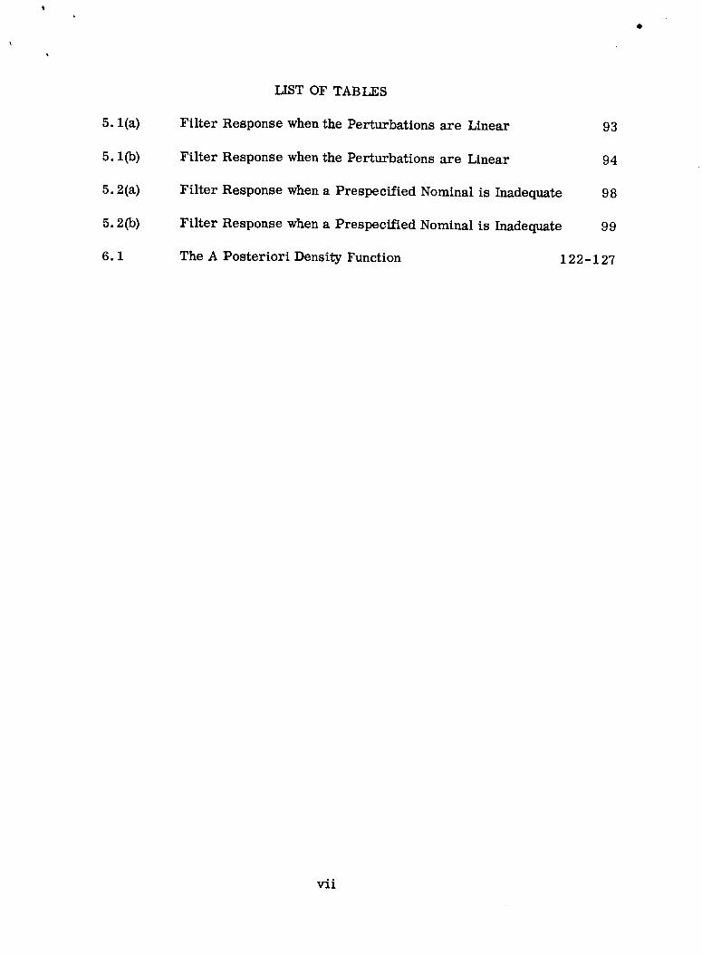
LIST OF TABLES
Filter Response when the Perturbations are Linear 93
Filter Response when the Perturbations are Linear 94
Filter Response when a Prespecified Nominal is Inadequate 98
Filter Response when a Prespectfied Nominal is Inadequate 99
The A Posteriori Density Function 1 22-127
vii

aq
-fk
h-k
1
_N-k
iJk
M0
Pk/k+y
NOMENCLATURE
expected value of the initial state
quantity describing the nonlinear measurement effects when
expressed in terms of the state x k
quantity describing the nonlinear measurement effects when
expressed in terms of the centered variable _k = Xk - _k"
The _k represents the conditional mean provided by a linear
approximation.
function that relates past and current state:
= !k(Xk_ 1, Uk_1, k_l)
function that relates measurement and state:
z k = hk(__ k, v k)
linear observation matrix containing the first partial
derivatives of h k with respect to x k
the i th Hermite ' "_olynuiill_t
criterion for establishing the optimal control at tN_ k. The
optimal control is chosen to minimize the conditional
expectation of _x_N-k
the second order observation matrix containing the second
partial derivatives of h k with respect to the state x k
covariance matrix for the initial state
eovariance matrix of the a posteriori density function of the
state x k conditioned on the measurements zk +¥
viii
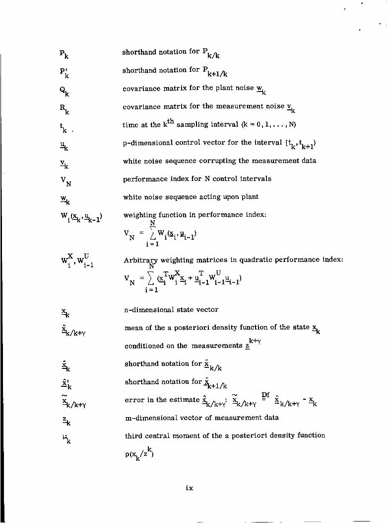
Pk
!
Pk
%
R k
t k .
V N
W_i ,wiU_l
_k/k+¥
shorthand notation for Pk/k
shorthand notation for Pk+l/k
covarianee matrix for the plant noise -_k
covariance matrix for the measurement noise -Yk
time at the k th sampling interval (k = O, 1,..., N)
p-dimensional control vector for the interval [t k, tk+l)
white noise sequence corrupting the measurement data
performance index for N control intervals
white noise sequence acting upon plant
weighting function in performance index:NV_
VN = LWi(xi'ui-1)
i=1
Arbitrary weighting matrices in quadratic performance index:
=Zi=1
n-dimensional state vector
mean of the a posteriori density function of the state _k
conditioned on the measurements zk +Y
shorthand notation for _k/k
shorthand notation for __-Xk+l/k
^ _ Df ^
error in the estimate _k/k+y: _c/k+y = Xk/k+¥ - _k
m-dimensional vector of measurement data
third central moment of the a posteriori density function
p%/z
ix

_k
I
5kj
_( )
exp( )
( )k
(_)
(_)k
( )*
( )T
-i( )
p( )
p(a/b)
<o( )
E( )
E(a/b)
(of
8f i
Dfa = b
fourth central moment of the a posteriori density function
p%/z5
identity matrix
Kronecker delta
Dirac delta function
exponential function
the quantity ( ) at t k
the quantity ( ) is a vector
the collection (_)1' (-)2"" (-)k
the nominal value of ( )
the matrix transpose of ( )
the matrix inverse of ( )
the probability density function of ( )
the conditional probability density function of a given b
the characteristic function of ( )
the expected value of ( )
the expected value of a given b
the matrix of partial derivatives of the components fi of f
taken with respect to the components x i of x
the matrix of second partial derivatives of the i th component
of f taken with respect to the components x i of x
the quantity a is defined to be equivalent to b
X

ABSTRACT
The problem of determining optimal estimation and control policies from
noisy measurement data for time-discrete, stochastic, dynamical systems is
considered in this dissertation. The method that is proposed here for the
solution of these problems represents a generalization of the common approach
that is based on the application of linear theory. In applying linear theory, it
is assumed that the state and measurement perturbations of the actual system
relative to an arbitrary system can be described by linear equations. Then,
it is possible to apply well-known linear techniques to estimate the state
perturbations and to determine the desired control corrections. In this
investigation, terms of higher order than first are retained in describing the
perturbations. The determination of estimation and control policies for the
resulting nonlinear systems is then accomplished within the framework of the
so-called Bayesian approach.
The general solution of the estimation and control problems can be
a posteriori density function p(xk/Z_ of the state conditionedestablished if the
upon all past and current measurement data is known. It is not possible to
express this density in a closed-form in most cases, so a principal concern
in this study is with the approximation, rather than the precise determination,
p(__/z_. A general procedure for approximating the densities is proposedof the
and then applied to a specific nonlinear system. For this system, the plant and
measurement noise is assumed to be additive and gaussian. Then, the a
posteriori density is approximated by a truncated Edgeworth expansion that
includes the fourth central moments. Using this form for the approximation,
xi

recurrence relations for the moments of the distribution are developed.
These equations can be simplified in a straightforward manner to yield several
other approximations. This includes a gaussian approximation that is more
general than the results obtained by first assuming a linear model.
The estimation problem was considered in some detail. Techniques are
suggested that allow the range of applicability of linear theory to be consider-
ably extended. This extension is illustrated by numerical examples in which
the estimates obtained from the standard Kalman filter, modified Kalman
filters, and the nonlinear filters are compared. The proposed modifications
are seen to yield significant improvements in many cases. These results
suggest that for many problems it might be fruitful to explore these and other
modified linear techniques before attempting to apply a nonlinear theory.
However, problems do exist that require the use of nonlinear methods. The
approach suggested here leads to results that are reasonable for use with
digital computers and appears to warrant further investigation.
xii

CHAPTER ONE
GENERAL DISCUSSION AND PROBLEM STATEMENT
The Austrian physicist Ludwig Boltzmann is reputed to have once
remarked that "there is nothing more practical than a good theory". Believing
this aphorism to be a worthy engineering watchword, it is the intent in this
study to investigate the problem of establishing estimation and control policies
for stochastic dynamical systems by considering a general theory, namely, the
so-called Bayesian approach. As with many such pithy statements, one or
more words can be subject to diverse interpretation. In Boltzmann's phrase,
the key word would appear to be "good", and we suggest that for many engineers,
it might be defined in the following, almost circular, manner. A theory is good
if it leads to the understanding and solution, either analytically or numerically,
of practical problems. Thus, after formulating the general problem and theory
in Chapters 1 and 2, considerable emphasis is placed upon the application of the
theory and the development of computatiunal a_uL.......... _dm_.
In Section 1.1, the mathematical model and the general problem are
stated and many of the terms and notations that appear throughout the text are
introduced and discussed. Results that have appeared in the literature relative
to the general topic considered in this study are reviewed in Section 1.2. This
discussion can by no means be considered to exhaust the subject. Additional
references appear throughout the text. In the final section of this chapter, the
theory that is proposed here for the solution of the estimation and control prob-
lems is presented. Also, an outline of the contents of Chapters 2 through 8 is
provided.

1.1 THE GENERAL PROBLEM
As has beenstated, the problem of determining estimation and control
policies for stochastic dynamical systems is to be considered. Before stating
these problems, several terms needto be defined.
First, it is important to recognize the precise meaning of "stochastic"
as used here. Certainly, it implies the probabilistic nature of the investiga-
tion but, moreover, we use it to imply that the a priori distributions of all
_random quantities are completely known. In this sense, we follow Bellman
[ 1, 2] who has suggested that a system be called adaptive when parameters of
the distributions are unknown and must be "learned". This is in contrast to
the case in which a parameter of the dynamical system is unknown but has an
a priori distribution that is completely defined. This example would still be a
stochastic problem, although the parameter must be estimated (or learned}.
Only N-stage, time-discrete systems are considered in the ensuing dis-
cussion. In general, the state [3] x k of the dynamical system is assumed to
evolve according to the nonlinear difference equation
x k = fk(Xk_l, Uk_l, Wk_l) k = 1,... ,S (I)
where the state x k is n-dimensional. The p-dimensional vector Uk_ 1 des-
cribes the control parameters that are to be selected according to a prescribed
control law. At each time, the system is disturbed by the random noise Wk_ 1.
k-1Throughout the discussion, the sequence* w is assumed to have a known
k* The notation a is used to designate the collection a(ao, a 1 .... ,ak).
probability density p(__...-1)t_and to be independentfrom one sampling time to the
next. That is,
P W(-_'o'Wl' ,.W_k) Df (w__... = p :
Sequences having this characteristic shallbe referred to as white noise
sequences (notto be confused with white noise processes which have a con-
siderably differentcharacter).
The notation that is used follows Fel'dbaum [4-9] and has the disadvan-
tage that the argument of a function serves a dual purpose. Itis used to name
the function (as is done above) and is also treated as a variable name (e.g., it
is treated as the variable of integration). The meaning should be clear from
the context.
The initialcondition for the statex is also a random variable with a_O
known probability density px(_xo).Note that the probability density is assumed
to exist in this and all other examples. This does not represent a significant
restriction and could be replaced in each instance by the Radon-Nikodym deri-
vative. The x is assumed to be independent of the noise sequences inthe-o
plant and measurements.
The function f--kin (I)is considered to be known. This relation is fre-
quently referred to as the plant equation and the fixed system that defines f-k
as the plant.
The behavior of the plant is generally observed imperfectly through the
measurement of quantities _ that are functionally related to the state variables
and which contain random errors.
the known relation
These data are assumed to be described by

Zk = hk(Xk, Vk) k = O,1,...,N-I (II)
where z k is a m-dimensional vector. The noise v k is supposed to be a mem-
ber of a white noise sequence with known density P(Vk).
Equations (I) and (II) constitute the basic mathematical model for the
study. Note that equations that are deemed to be of particular importance shall
be denoted with the Roman numeral as has been done for (I) and (II). Arabic
symbols shall be used for equations having a more secondary nature. The
subscripts E and C will be used for equations that are significant for either the
estimation or the control problem, but not both.
It is now possible to give a more explicit definition of the estimation and
control problems.
ESTIMATION: The estimation problem is essentially concerned with the
k+¥determination of the state x k from the measurement data z The problem
separates naturally into three subproblems.
1) Filtering: estimate x k from all past and current measurement
data zk (i.e., ¥ = 0)m
2) Prediction: predict x k from past data (i. e., ¥ < 0)
3) Smoothing: estimate x k using future data as well as past and
current data (i. e., y > 0).
All three cases shall be dealt with in the succeeding pages, but the greatest
emphasis is placed upon the filtering problem. In particular, we shall con-
sider the recursive filtering problem in which the estimate _-k shall be based
upon _k-1 and z k.
4
Because of the presence of noise in the plant and measurement equations,
it is, in general, not possible to determine x k precisely from the data zk +Y.
Instead, the estimate _k/k+y must be chosen to approximate x k in some well-
defined sense. Suppose the error in the estimate is denoted as Xk/k+ ¥ and is
defined as
~ WXk/k+y k/k+y
The error criteria that is selected generally has the form of E{_(Xk/k+ _ ]
where _ is positive and spherically symmetric. That is, it is true that
and such that if
then
_a e_a
0 < %0(Xk/k+¥) = _(-Xk/k+ Y)
x ( )-k/k+y ]Xk/k+¥
.,-_(i) , ~(2)
%0(Xk/k+)) _ ¢P(Xk/k+ _)
Examples of error criteria that satisfy these conditions are:
1) Minimum mean-square error.
For this criteria, the estimate is chosen to cause
E[__T "_ k+y]k/k+¥ Xk/ = minimum.
2) Minimum absolute deviation.
In this case the estimate is chosen so that
[ l k/k+¥1 I = minimum.

It is well-known and will be demonstrated in Section 2.1 that the mean
square error is minimized by choosing_k/k+y to be the mean of the conditional
p(.X_k/k+Y). It is also known [10] that in the scalar case the minimumdensity
absolute deviation is obtainedby choosingthe estimate to be the median of
k+7p(xk/z ).
For the scalar case, Sherman [11] has pointed out the following lemma.
LEMMA: For the rp defined above and if P is a probability distribution on the
reals which is symmetric and unimodal with mode at the origin so that P(X) =
1 - P (-X) at each continuity point of P and P is convex for X ,_ 0, then
J%(x) dP(X) - a) dP(X)
for each real a, when the integrals exist; if either integral diverges, the one
on the right does.
This implies that for conditional distributions satisfying the conditions of
the lemma, the estimate for error criteria E[r_ (Xk/k+_)] is the same as for
the minimum mean-square error criteria. Thus, estimates based on the latter
criteria can encompass a much larger class then is popularly believed. For
the remainder of this discussion, only mean-square estimates shall be con-
sidered. Thus, the estimates will be selected to minimize
-_ _-T _- (IIIE)_(Xk/k+¥) = E [ Xk/k+ ¥ Xk/k+y]
An additional criteria for selecting the estimate would be to select
_k/k+y as the maximum value of the conditional density function P(xk/k+Y ) .
This is sometimes referred to as the "most probable" estimate and is the mode
of the distribution. Cox [12] has considered this estimate in considerable detail.

It has the disadvantage that there is nonatural measure of error to attribute to
the estimate.
CONTROL: The plant (1)is causedto behavein a particular manner through
N-1the selection of the control vectors u . The rule according to which the u k
are selected at each sampling time (k = 0, 1 .... ,N-l) is called the control law
for the system. As was true in the choice of estimates discussed above, the
means of establishing the control law is somewhat arbitrary. In the following,
we shall assume that the control is chosen to minimize the expected value of
the performance index
N
V N =_ Wi(x i, ui_ 1) (IIIC)
i=1
The W. are specified functions of the state and control variables and shall be1
required to be nonnegative and spherically sysmmetric. A familiar example and
one that will be used later is the quadratic index
N
T wXx + T UVN = _ (xi _ -i Ui-lWi-lUi-1)
i=1
where the ¢ and W Ui-1 are arbitrary, non-negative definite weighting matrices.
kThe behavior of the system is observed through the measurement data z
so the control law is taken as a function of these data. That is, at each sampl-
ing time tk, to g tk a tN_l, the control is computed according to
u k = U k [ ?-Y]
The y has been included to indicate that the control might be based on
past data only. Physical realizability considerations require that y > 0 since
the control could not be expected to depend upon fftture measurements.
7

It would appear that a more general control law could be obtained if u k
were allowed to be a random {rather than deterministic} function of the meas-
urement data. Fel'dbaum considered this possibility and found [5] that the
generalization did not provide any benefit in the cases that he considered.
Sworder [ 13, 14] has shown that it is sufficient to consider deterministic con-
trol laws for Bayesian control policies.
The form of the optimal control law for a given system {I) and perform-
ance index (IIIc) depends upon the nature of the observational information that
is assumed to be available to the controller. The two conditions that are of
greatest interest occur when ¥ = 0 and when ¥ = k. The former results in a
feedback (or closed-loop} control law, whereas the latter leads to an open-
loop control law. In deterministic problems, there is no difference between
the two types of control.
In open-loop control, the entire control policy is established by the
initial conditions whether this is represented by x or measurements made' _O
prior to the initiation of control. This can be modified to a policy that has been
referred to as an open-loop feedback control law. In this case, the control
policy is computed anew at each t k by treating t k as the initial time and by
ignoring the fact that new data will be available at later times. Open-loop,
feedback control might be expected to produce a policy that is superior to open-
loop control but inferior to feedback control. Dreyfus [ 15] demonstrated that
this intuitive idea is valid for a simple stochastic control problem. Katz [ 16]
shows that the feedback policy provides a lower bound for the value of the
performance index when the systems are time-continuous.
8
A fourth alternative has beensuggestedby Simon [ 17] and has been
called a certainty equivalence control policy. In this case the random variables
are replaced by their unconditional mean values and the problem is treated as
deterministic. This policy has been shown to provide a solution to the stochas-
tic control problem for linear systems containing white noise sequences and with
a quadratic performance index. This situation is discussed in Chapter 3.
The problem of determining feedback control policies is considered in
Chapters 2 and 3.
1.2 PREVIOUS RESULTS
Research into the stochastic control problem has quite naturally taken
two avenues of approach. In the preceding section, the problem has been posed
in terms of a time-discrete system involving difference equations and a finite
number of observation and control times. It could reasonably have been stated
instead in terms of a time-continuous system with a differential equation model
and continuous measurement and control processes. Since dynamical systems
are usually described by differential equations, it could be concluded that this
would be the more natural model. A considerable amount of research effort
has been expended in this area. For a summary, see References 18 or 19.
More recent results than those described in the aforementioned references
have been published by Buoy [20], Bass [21], Mortensen [22], and
Fisher [23]. The first two have dealt with the estimation problem, whereas
Mortensen has presented a very general and mathematically sophisticated
solution of the control problem. Fisher considered the estimation problem

from the point of view of approximating the a posteriori density function of a
time-continuous system.
There are advantages and disadvantages to both formulations. The
principal disadvantage of the time-discrete model arises from the fact that, as
has already been mentioned, a dynamical system is generally described by a
system of differential equations. In order to obtain the time-discrete model,
it is necessary to reduce the system to the form described by (I) and this
requirement engenders a problem of considerable significance. On the other
hand, it is believed that the formulation presented in Section 1.1 is more
realistic for several reasons.
(1) Measurement data are usually available only at discrete times.
(2) In many complex systems, the control is determined with the
aid of digital computer so the control is changed at discrete
times.
(3) In the time-continuous case, white noise processes are generally
assumed to act on the plant and measurement process and such
noise is physically unrealizable.
(4) Last, and not least, the general solution of the time-continuous
estimation and control problems yields systems of complicated
partial differential-integral equations that must be solved. The
difficulties inherent in obtaining numerical solutions to practical
problems using this formulation appear to be excessive.
10

When(1)and (II) are linear, the noise is Gaussian, and a minimum mean-
square error criteria and a quadratic performance index are utilized, the
solutions to the estimation and control problem are well-established. There
have been manyworkers in this area, but many of the better known results have
been attributed to R. E. Kalman [24,25,26]. It was suggestedby Kalman and
Koepcke [27] that for linear systems the estimation and control problems
could be considered separately. That is, the estimates canbe computedas
though the control is a knownfunction of time and the control law found for the
deterministic problem canbe used for the stochastic control law. The control
is computedaccording to
Uk = Ak_k
where hk describes the deterministic control law, and _k has replaced x k•
This result has been stated as a "Separation Theorem" andwas first proven
independentlyby Gunckel [28] and by Joseph [29].
For nonlinear systems, an approachthat is commonly used in practice
involves the use of linear perturbation techniques [30]. First, a nominal or
reference solution of (I) is assumedto exist that provides a "good" approxima-
tion to the actual behavior of the system. The approximation is "good" if the
difference 5x betweenthe nominal andactual states canbe accurately described
by a system of linear difference equations
6x k = _k,k_15Xk_l+Fk,k_lUk_ l+Ak,k_ lwk_l
and the difference in the measurements 6 z k is given by
11

6z k = Hk6X k + v-k
This approach has yielded many satisfactory results, but several weak-
nesses have become apparent. For example,
(1) There is no easily obtained criteria for judging the validity of the
linear approximations.
(2) The filter does notbehave satisfactorily when the measurement
noise is small. Pines and Denham [31] have attributed this to the
absence of second order terms in the expansion of the measure-
ment equations.
(3) This procedure lacks generality. It provides little insight into the
techniques for considering more general systems.
It has been suggested by several people that it would be more appropriate
to formulate the problem in terms of the a posteriori density function p_k/zk).
In a series of four papers, Fel'dbaum [4 -7] dealt with the control problem
and derived several basic results. Ho and Lee [32] considered the estimation
problem. Aoki [33] has conducted an extensive investigation of both problems.
These results are contained in his forthcoming book. In an excellent doctoral
dissertation, Sworder [13, 14] has considered the control problem using a
game-theoretic formulation. Stratonovich [34] dealt with the a posteriori
density for time-discrete and time-continuous systems.
P(Xk/zk ) theoretically provides the solution to both theKnowledge of
estimation and control problems. The estimates _k and control u k are
required at each sampling instant so it is necessary to know P(Xk/Z k) for
12

every tk.
according to the recursion relation
It is not difficult to show (see Chapter 2} that P(Xk/Z _ evolves
where
and
p(_xk/zk -1)
P(Xk/Z _ =
k-1
P(Xk/Z )P(Zk/X k)
z /z k-1P(-k - )
k-1= ._p(_xk/g )P(_-k/Xk_l,Uk_l ) dX-k_ 1
p(__k/k-l)
The denominator of (IV) does not involve x k
(IV)
constant.
= _p__k/k-1)p(z_k/Xk ) dx_k
and plays the role of a normalizing
The general concept of dealing with the a posteriori density is referred
to as the Bayesian approach to estimation and control. Unfortunately, it is not
possible to solve (IV) in closed form for most problems. (The major exception
occurs for linear systems.) Furthermore, the computational requirements
for solving (IV) numerically become astronomically large for almost any non-
trivial problem. Thus, it becomes apparent that approximations must be intro-
duced that will reduce the complexity of the problem without destroying its
character.
i. 3 PREVIEW OF COMING ATTRACTIONS
Since one must know: P(Xk/zk) before proceeding with the solution of the
estimation and control problems, it is the intention in this investigation to
develop a means of approximating the density. It is believed that a combina-
tion of perturbative and Bayesian techniques will permit the development of a
13

theory that is at once more general than the linear theory but more computa-
The procedure that istionally attractive than the general Bayesian approach.
proposed for achieving this meld is described below.
(1) At each sampling time t k, nominal valuest for Xk_ 1, Uk_ 1, and
Wk_ 1 are assumed. Then the fk is expanded in a Taylor Series.
The measurement equation h k is expanded about fk _-1 u*' -k-l'
P(Xk/k) must be assumed. This form is required to(2) A form for
be true for all k.
(3) The a priori statistics for the plant and measurement noise and
the expansions of f-k and h k are introduced into (IV). Only those
terms are retained that yield the desired form for P(Xk/Zk).
The application of this procedure to a system leads to several questions
concerning the resulting approximation.
(1) Does the approximation describe p_k/Z k) accurately enough to
have confidence in the validity of the estimation and control policies
that are subsequently derived7
(2) Does the approximation lead to estimation and control policies
that provide a significant improvement over linear policies7
A question that is related to the preceding one can be phrased in the
following manner.
t nominal values are denoted by the superscript *
14

(3) Can special techniques be developed that extend the range of
applicability of linear theory and thereby eliminate the need for
nonlinear considerations in many problems ?
In this study, several specific approximations are developed. Then,
these questions are considered by examining the estimates of the state of a
dynamical system that are obtained from the approximations. This is accom-
plished through digital simulation.
In Chapter 2, the general Bayesian approach is discussed. The solution
of the minimum mean-square estimation problem is shown to be the conditional
mean. Conditions that the control must satisfy for the performance index (IIIc)
to be minimized are derived in terms of the a posteriori density. Then,
equations which describe the a posteriori density p_k/k+¥) (for any integer ¥)
are derived. These results have appeared [33,14, 32,35] before in the litera-
ture. In addition, the relations describing the p(_k/k+¥) are rewritten in
terms of characteristic functions. It has been found in Chapter 3 that the
characteristic function formulation can reduce the amount of algebraic manipu-
lation required in the solution of a problem.
The Bayesian approach is applied to the linear stochastic control problem
in Chapter 3. It is used to obtain the Kalman filter equations [24,30 ], Rauch's
smoothing equations [36], and to prove the Separation Principle. It is seen
from the proof that the Separation Principle is valid because the error covari-
ante matrix for this case does not depend upon the measurement data.
15
The procedure stated at the start of this section is applied in Chapter 4
under the constraint that P(Xk/Z_ is Gaussian. It is demonstrated that the
filter equations that are obtained are no_._tthe linear Kalman equations. Instead,
second order terms appear and the conditional covariance becomes a function
of the measurement data. This is a distinct departure from the Kalman filter
in which the conditional covariance is independent of the measurements. It is,
however, characteristic of nonlinear estimates. It is further observed that a
distinct simplification in the filter is obtained by requiring the nominal value
for _k-1 to be _k-l" The control of a linear system with nonlinear measure-
ments is considered, and it is suggested that the Separation Principle is no
longer valid.
The problem of estimating the state of a spacecraft moving in a nearly
circular, 100 nautical orbit about the Earth from horizon sensor measurements
is considered in Chapter 5. A digital computer program simulation was set up
to simulate the physical system and the techniques and results obtained in
Chapters 3 and 4 are utilized. The linear filter of Chapter 3 and the nonlinear
filter of Chapter 4 are compared. In addition, techniques for extending the
range of the linear filter are proposed and used. Several interesting con-
clusions are suggested by these numerical results.
In Chapter 6, attention is restricted to the nonlinear estimation problem.
In this chapter, the a posteriori density is approximated by a truncated
Edgeworth expansion. All considerations are limited to scalar plant and
measurement equations, and approximations retaining third and fourth order
16

conditional moments are derived. It is seen that the approximation is achieved
by developing recurrence relations for the moments of the distribution.
The results of Chapter 6 are applied to a simple problem in Chapter 7.
Filters based on a linear theory are exercised and compared with the filters
produced by the approximations. "Modified" linear techniques are also
examined.
The major results and conclusions provided by this study are summarized
in Chapter 8. The contents of each chapter are described in Section 8.1, and
the reader might consult that discussion before proceeding through Chapters 2
through 7.
17

PRECEDI_Q P_B BLANK. NOT' FIL_ED.
CHAPTER TWO
THE BAYESIAN APPROACH
In the so-called "Bayesian approach" to the problems of determining
estimation and control policies for stochastic systems, one is concerned first
of all with the determination of the a posteriori density function P(xk/k+Y).
This density function provides all of the data required for the solution of these
problems. To see that this is indeed the case, the following section shall be
devoted to the solution of the minimum mean-square estimation problem and
the optimal control problem. In this discussion, it is assumed that the nec-
essary density functions are available. The solution of these problems provide
a means for determining "best estimates" and "optimal controllers" if the
P(Xk/z_k+Y } is known. In Section 2.2 it is demonstrated that the a posteriori
density can be determined from the a priori statistics specified for the plant
and measurement noise. Naturally, the functions fk and h k enter these con-
siderations. In the concluding section of this chapter, the relations describing
the a posteriori density are rewritten in terms of characteristic functions.
Reference will be made frequently in this and subsequent chapters to
three properties of conditional density functions [ 37 ].
1. For random variables a and b with joint probability density
function p(a, b_), the conditional density of a, given b, is defined
as
p(alb__) - p(a, b) _:p(b) (2.1)
19

2. For random variables a, bb_, andc_,
p(a, b_l_c)= p(blc) p(alb_, c) (2.2)
This is known as the chain rule.
3. For random variables a, b_, and c,
p(__h) -- _p(__lb_,c) p(b__) db (2.3)
This is the integrated form of the chain rule and represents one
version of the Chapman-Kolmogorov equation.
Note that the definition of conditional densities (2.1) can be rewritten as
p(alb) = p(b_la_) p(a_) (2.4)p(b_)
This relation is known as Bayes' rule and is the source for the term Bayesian
as used in this and other chapters.
Note that the integration indicated in (2.3) involves vector variables.
The single integral sign will be used for both scalar and vector variables and
db_ will be used to describe the differential dbldb 2. .. dbn. When more than one
vector is involved, the differential will be written as d(a, b,... ,z).
2.1 OPTIMAL ESTIMATION AND CONTROL FOR STOCHASTIC TIME-
DISCRETE SYSTEMS
The mean-square estimation problem and the optimal control problem
shall be solved in this section in terms of the a posteriori density function.
2.1.1 The Minimum Mean-Square Estimation Problem
The solution of the minimum mean-square estimation problem [ 38 ] is
provided by the following lemma.
2O

LEMMA 2.1: Suppose that a random variable x is to be estimated from the
known variables* zq. The x and z2 have the joint probability density function
p(x, zq). The estimate _¢ is to be chosen as a function of the zq so thatD
^ ifEl(x- x) T - x)] = minimum
Then, the mean-square estimate of _ is
= E[xi q] (VE)
Proof: Write E[(_ - x)T(_ - x)] in terms of the joint density function.
E[(_-x)T(:_-x)].....: ,;(_-x)T(_-x)p(x,zq)d(x,z q) (2.5)
From (2.1), the density function can be written as
z2) = P(x/zq)p(zq)
Thus, (2.5) is equivalent to
E[ (_ - x)T (__ _ x)] = f[_(_ - x)T (__ _ x_)p(_x/zq)dx_ j p(.z_q)dzq
Consider the integral in brackets. Since _ depends only upon the zq,
the integral can be written as
.;(__- x_)T (_ _ x_)p(_x/zq)dx_^T^
= x x- 2xT Etx/z q] + EtxTx/z q]
= (__ E[x_jzq] )T(_ _ E[x/zq] ) + E[xTx/z q]
- [ E [x__/zq] ] TE [x_Jzq] (2.6)
By definition this quantity is positive, so to minimize E[(_ - x_)T(_- x)], it is
sufficient to minimize (2.6). Only the first term involves _, and the smallest
value that it can assume is zero. Thus, the minimizing estimate is given by
f = E[x/z q] Q.E.D.
* Recall that the set _1' z2'"" ,Zq) is denoted by zq.
21

This lemma shows that the conditional mean provides the mean-square
estimate of x. Certainly, if one knows the a posteriori density functionm
p_/z_q), then the estimation problem has in principle been solved. Other
estimates such as those given by the mode or by the median of the distribution
are also established from knowledge of pi_/zq).
The conditional mean provides an unbiased estimate of a variable x.
That is, it is true that
E[x] = E[_].
This is verified in the following manner.
By definition, one has
Eta) = ,F p %dzJ
But _ is the conditional mean, som
Eta] = .[[_x_p_./zq)dx_} p_q)dz q
From 2.1, it follows that
EEJ = Iw _,
Integrate with respect to zq. Then,
E[__]= ]'__p_
Df= E [x]
2.1.2 The Control Problem
N-1Suppose that a feedback control policy u is to be determined for the
system (I) and (II) that minimizes (HIc). It shall be shown that
LEMMA 2.2: The optimal feedback control policy for the system (I) - (II) and
performance index (IIIc) is the control that causes
22
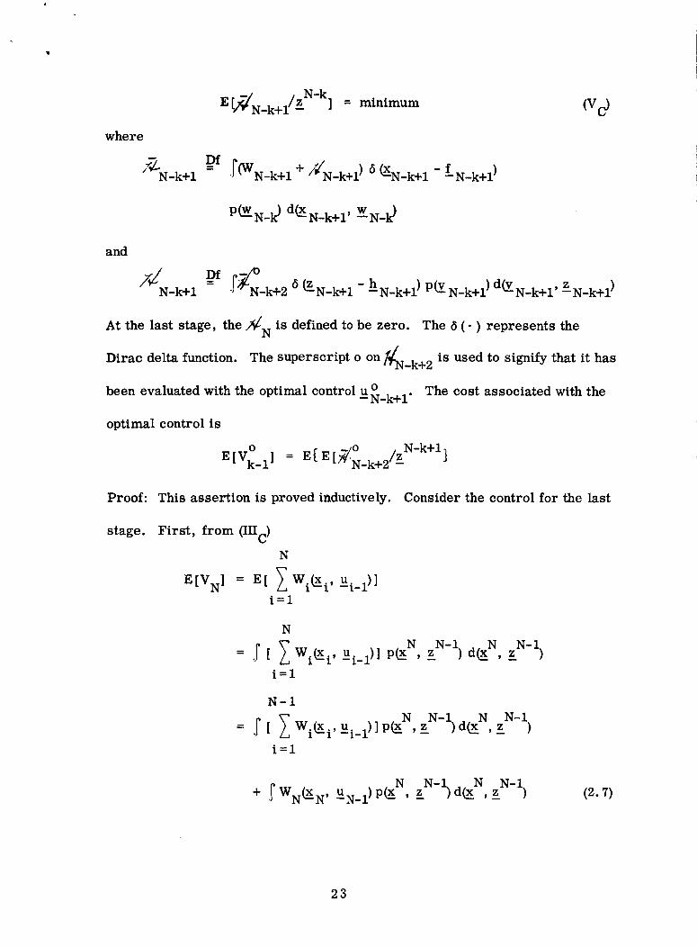
- N-kE [2_/N_k+l/z ] = minimum
where
_,_-_+1=_,r%-k+_+%___+_)_%__+_-
P(_'N-_ d(-_N-k+l' WN-_
and
1_N_k._ D_r_= ' -k+2 6 (_-N-k+l
(vC)
f-N_k+l )
- hN_k+ I)P(-ZN_k+l )d(Y-N_k+ I,ZN_k+ I)
At the last stage, the/V_ N is defined to be zero. The 6 (-) represents the
Dirac delta function. The superscript o on if-N-k+2 is used to signify that it has
been evaluated with the optimal control o The cost associated with theUN_k+ I"
optimal control is
o _/o . N-k+l _E[Vk_l] = E{E[?CN_k+2/z J
Proof: This assertion is proved inductively. Consider the control for the last
First, from (IIIc)
N
E[VN] = E[ lWi(_i' Ui-l) l
i=l
N
t[ Zw_c_,u___>]pc_", z2-_>d__,z2-_)i=1
stage.
N-1
; [ Zw,_.,,u,_l>)p=_,_z_-l>d_.N,___-_>i=1
+ [ WN(_XN ' UN-I )p_N, _zN-l)d(_x_N,_zN-I) (2.7)
23

N-1
The integrand of the first term does not contain x N or z , so an integration
will eliminate these variables. The control UN_ 1 enters only the last integral
so no other terms need to be considered in determining the optimal control for
the last stage. Let
E[Vll =Dr _WN(_N ' UN_l)P(xN, _zN-1) d(x- N, _zN-l) (2.8)
N-Using the integrated chain rule (2.3), p(N, z % can be written as
peN,__N-1)= p_N/xN-l_,__N-1)p_N-1,z_N-5
p(_N-1 N-1 s - N-1 N-1= ,z )Jp(__N/X ,z ,WN_l)
p(_wN_i/xN-l, d-l)dw N_ i
But WN_ I is a white noise sequence, so
p(__N_i/d-i N-I,z ) = p(EN_I)
N-1and since z defines UN_ 1, it is clear from (I) that
N-1P(__N/X:-I, z ,WN_ I) = p(__N/XN_I,UN_I,WN_I)
= 6(_N-L N)
where 5 (") represents the Dirac delta function. Thus,
Substituting this into (2.8), E iV1] becomes
= __ ,_ ,W_N__)
Let
N __Dr._WN(.X_N,UN_I)6 (_N - f--N)P('V-N-I)d('_N'WN-I)
24
Then
E[VI] N-I N-l)_.-_NP(__N_I,z )d(._N_l,Z
where the integration with respect to Nx__-2 has been performed.
further modified to
_.tv_ = ;_;_%_/zY-_)%__C_"-I)dzY-_0
The E [Vl] will be minimized by the control UN_ 1 that causes
[ _N/Z N-l] = minimumE
= 1,This verifies (Vc) for k
oUN_ 1 by so that
This can be
Denote the value of >_N that is evaluated with
(2.9)
0 o
Suppose that the optimal controls UN_k+l,... ,UN_ 1
ing to (Vc) and that the expected cost associated with these (k-l) stages is
Then, using the Principle of Optimality, it follows that
_.tvkl= ;W,__k+_%__+ru,__k_'_-_+_,z'%dC_N-_+_,z'%_o
+ E [Vk_l]
Let us rewrite the second term
o_ = j_fgN_k+2P(_X_- o N-k+l, _zN-k+l) d(.N-k+l, _zN-k+l)EtV k 1]
are computed accord-
(2.10)
25

But
z N-p(_N-k+l__ k)_ , N-k+l N-k= Jp(Z_N_k+i/x ,z ,VN_k+ i)
• , N-k+l, z_N-k)dv_N_k+lP(Y-N_k+I/x
From the assumption on the noise and from (II), this reduces to
p_N-k+l, zN-k+l N-k+l, zN-k) _5_ ) = p(x _ (9-N_k+ 1 - hN_k+ 1)
P(Y-N_k+l)dVN_k+ 1
O
Using this result, E[Vk_I] becomes
o _ o N-k+l N-E[Vk_I ] = :_S_k+2 5 (Z_s_k+l - hN_k+l)p(y_N_k+l)p(_ _ /z
N-k+l, zN-k+l).d(.ZN_k+I,x
Let
Df o-- F N_k+26 N-k+l - hN_k+l)p (y_N_k+l)d(.VN_k+1,ZN_k+ I)
So
,z N-O _ N-k+l, zN-_dC-k+l - k) (2.11)E[Vk_ll = J/_N_k+lP(_X_ -
Introducing (2.11) into (2.10) yields
, N-k+lE[Vk] = _(WN_k+ 1 + __k+l)P(__
Proceed as was done to obtain (2.9).
N-p_N-k+l,z k) = p( N-k
, N-
It follows that
N--
,z k) 16(XN_k+ 1 _ fN_k+l)P(.W_N__dWN_k (2.12)
26
Let
so that
Df
P (-_.N_k'x--.N_k+l)
E[Vk] = j N_k+iP(_N_k, - _ _
f'[eZ,_ x .zN-kdx - zN-k N-k= J J. N_k+iP(XN_k/Z -_ ==N_kJp(9_ "_dz
The optimal control must satisfy (Vc) and the cost is
.-_ . N-kE[V_] = E[E[._N_k+I/Z ]}
This completes the proof of the lemma. Q.E.D.
The optimal feedback control problem has been solved in principle if the
a posteriori density pQxk/z_ is known for all k. Similar results can be found
in [5,13,33].
2.2 THE A POSTERIORI CONDITIONAL DENSITY FUNCTION
In the preceding section, it was shown that the a posteriori density func-
tion provides all of the information required to determine optimal estimation
and control policies. In this section, equations governing the structure of
p_k/k+Y) shall be derived.
2.2.1 Recursion Relation for p_k/Z_5
density p(__/z_ can be described by an integral recurrence relation.The
This fact shall be stated as a lemma and then proven.
27

LEMMA2.3: For the system (I) - (II) and a non.randomizedcontrol policy, the
a posteriori density function p(_._._/z?}evolves according to
• "zk-I p z /p%/_ )%_)p_/k) = _/_k-1 (Iv)p%_ )
where
/ /z k-1= JP% __:r:_--,)P%-_- )¢%-i (2.13)
and
pz(.zk/z_k-:l" ) = _p(_y__/z_k-1)pz(z,k/.X::k)% (2.14>
The initial condition p x(X.o/Z) is given by
P z(.._/.._,o)P x(.._ )
p%/Zo) = P%) (2.15)
where
p%) = .i'p%/+.,:,)pmo)__o
Proof: The initial condition can be established directly from Bayes rule (2.4).
Thus, consider arbitrary k.
From the chain rule (2.2), one sees that
k-1p%,__/z_+ ) = p%/z_pz%/_"I)
SO
p%,_/zJ-_)
But the chain rule also enables us to write
28

%/z )= P%_k- )P%-)pt_, k-1 _ / ,,k-1 /zk-1
This can be simplified to
p(_xk, Z_k/zk- 1) k-1_ : p_l_p_lzL )
since, from the noise assumptions in (1) and (I1), it is true that _k given Y_k is
k-1independent ofz . Thus,
P_k/k- 1) p_/y_k )
k-1 (IV)
p%/_ )
This relation proves (IV). It remains to verify (2.13) and (2.14).
From the integrated chain rule (2.3),
k-1P%/z_ ) = _P%/_kr zk-1 /_k-1_- )PLy_l- )_-1
But zk-1 defines _k-1 so
k-i , k-ip%/_ )= fP%/_k_l__l)P%_l/z _ )d%_1
The integrated chain rule also allows one to write
=
This completes the proof. Q.E.D.
The p Z(Zk/z_k-i) in (IV)does not depend upon _k' so itcan be seen to be
nothing more than a normalization constant. The basic structure for the
recursion relation is provided by the numerator. Itshould be noted in passing
that itis not possible in general to perform the integrationindicated in (2.13)
k-ito obtain a closed-form for p(__/z _ ).
---K--
29

2.2.2 The A Posteriori Density Function for Prediction and Smoothing
Equation (IV) provides the basic formula for filtering and control pur-
poses. Occasions do arise when it is desirable to obtain predicted or smoothed
estimates of _k' so it is necessary to determine the density p_k/Z_ k+Y) for
y i_ 0. For this case the control variables will be eliminated thereby reducing
the plant equation to
LEMMA 2.4: For the system (IE) - (If),the a posteriori density function
/zk-Y_p(_xk _ _ fory>0 is
/zk-¥_d/-- ,p(_X__y _ , x___l ""'_k-_ (VIE)
The proof of this statement follows immediately from the repeated application
of the integrated chain rule. See the derivation of (2.13) for the case when
y=lo
The derivation of the smoothing density is somewhat more involved. The
result can be stated as follows.
LEMMA 2.5: For the system (IE) - (II) the a posteriori conditional densiiy
function p(___y/Z_ for y > 0 is given by
p%_¥/z5=/zy- , . . . ,
where p Z__k,...' z'--y+l/X'--y)_ --K is computed recursively according to
3O

p z(_,... ,._=¥+i/__y)
_%-y+,%-y)%-y+,
'' '"Z-k ....y+2/_k y+l)P z(=_k¥+i/_k y+1 )
(2.16)
The initial condition for this relation is (i. e., ¥ = 1)
Proof: The proof shall be inductive. Let ¥ = 1 and consider
_%__,_,___)= _%__._._j,_%_(_%k-i k-i k-i
= p%,%/___,__ )p%_J_ )pc_ )
= _,_/___)p__,/_-_pc_ _-_)
, • • / • - /zk-1 zk-1= P%/_k _k-_)P%_k-,)P%-i = )P(_ )
= p Z(Zk/Xk) p(xk/Xk _ 1)P% _ 1/zk- 1) P(.z_k-l)_
Furthermore, it is true that
p%_l,!ik, 5 = p%_l,Xk/zk)p__ k)
= ,c__,._/zS, z_/_-'),(_'-_)
Equating (2.18) and (2.19) and rearranging terms, one obtains
_%)_%%__)___/F _)p%_l,_k/_k) =
Integrate with respect to _k" Then
(2.17)
(2.18)
(2.19)
31

where, by the integrated chain rule (2.3),
This proves (2.16) and (VII E) for ¥ = 1.
Suppose that (VII E) and (2.16) are true for y = j-1 and let ¥ = j.
as for ¥ = 1. Then it follows that
p_,_j,__j+_,z_: p%.,,,._,_m/_,_j+?
P%-j+I/_k-j)P(-_-j/k-j)p_k-j)
and, also that
, zkPQ-Y-_-j'_k-j+l - )
Proceed
(2.20)
= P(-'xk-j'_k-j+l P )''"
p Z(Zk_j+l/k-J) p(z_k-j ) (2.21)
Equate (2.20) and (2.21) to obtain
p%-j/_-J)p%-j+l/_,-j)p% '''',_,-j+l/_,-j+?
_-J'_-J+J_) : _z%/z_k-J)..._z%_j+j_-J)
Integrate with respect to _k-j+l" Then
p%_/__k): _-{_-%_,-" ,_-m/_-j )_z%/z__-_)..._z%_j+j_-J)
where from the integrated chain rule, it is true that
pz%,..., __j+l/_,_j) : rpz%,... ,_,_j+l/_,_j+l)
p%_j+l/_-j)%-j+l
By the chain rule (2.2), it is apparent that
32

p%.,,,.__j÷J__m) : p%.,,,.__j÷2/__m)p%_m/__m)
This completes the proof of VII E and (2.16). Q.E.D.
2.3 CHARACTERISTIC FUNCTION EQUIVALENTS
Relations for the a posteriori conditional density function p(x,/z k+¥)
were derived in the preceding section. It is, of course, possible to obtain
from these relations their characteristic function equivalents. These relations
are to be derived and exhibited in this section. The characteristic functions
are introduced primarily for future reference. It has been found that in many
cases the problem solutions are most easily obtained using the characteristic
function formulation. The reader is encouraged to perform the derivations in
Chapter 3 by using the probability density relations of Section 2.2.
Recall that the characteristic function _ and the probability density func-
and
tion p associated with a random variable x form a Fourier transform pair [ 10].
1 :(e. 2el
J
LEMMA 2.6:
o_
p(_x) = --1 _ exp(-is-Tx-)_°(_) ds(_)n _oa
Consider the characteristic function for p(_.xk/zk )
Thecharacteristicf_ction_%) forp%/zk)is
as described by (IV).
1
n+m - k-1(m p%/__ )
• T T_exp[-' S_k/k-l-_k) _k- is__v -_k ]
cPs(._k/k_1)cP(-_v)d(-Y-_,_v, -_k/k_1) (viii)
33

where <0S(Sk/k_l)andW(_ are the characteristic functions associated with
p(__xk/zk-1)andpZ(Zk/!_k) , respectively. The characteristic function _0S(Sk/k_ 1)
is given by
i ]'e_pE-i% T T_ - __/k_1)_ -i_k_1__I(2TT)2n
(2.23)
where _p_) is the characteristic function associated with p_k/Xk_l,Uk_l).
Also,
z /zk-1 - i T _ iT k]Pz(_k _ ) (2TT)n+m _exp[-i_k/k-l_k
_%/k-1)_%)d% '_'_/k-1 )(2.24)
The characteristic function cOS(So)for pX(Xo/Z) is
v%) =(2TT)n+mpZ(_)
yexpI-i sC_u - s_o)Tx - i Tzol
(2.25)
The _ SCan) is the characteristic function for p_o ).
Proof: The proof follows directly from the definitions (2.22) and from (IV).
The characteristic function of p_k/k) is
=. T k-11 ;exp [ i .Sk _k ]P(_Y.xk/z )P Z_k/_k>dX- k
(2.26)
But
p(_yxk/zk-1 ) -(1)n.Fexp[-isk_k_l_Xk]CP S(Sk/k_l)d-Sk/k-1
(2.27)
34

and from (I1) it is clear that
-- 1 rexp[-isTz. ]_o(s)ds
(2_m " -v-x --v- -v
Substitute (2.27) and (2.28) into (2.26) and (VIII) follows directly.
The characteristic function _(Sk/k_l) is given by
._exp " T k-i= [ 1Sk/k_lXk] p_k/Z )dx_k_°(Sk/k_1)
But from (I)
P%/%-l'"k-1)
so from (2.13)
= 1 rexp[_isTx, ]¢p(s )ds
(2_)n _ -w-x _ -w
T1 _exp[-i s(_w- _k/k-1 ) _k - i'_k-Tiy_:k-1]
(2_) 2n
This proves (2.23). The p Z_k/zk-1)_
(2.28)
•
can be written in terms of characteristic
functions directly from (2.14). The characteristic function _ S(So) follows
immediately from (2.15) Q.E.D.
The characteristic function for the smoothing density follows immediately
from (VI).
(__/z_k-Y) for >LEMMA 2.7: The characteristic function equivalent of p y 0 is
T T= __y_fexp1 [-i S(_wk_1 - Sk ) _!k - iSwk_2_k_l]...
_°(Sk/k-_ (
(IX E )
T T
exp [-iSwk_¥Xk_¥+l - iSwXk_v]
d(-Xk_l,•••,_k_y,_wk_l, •••,_k/k_¥)
35

LEMMA 2.8" The characteristic function for the smoothing density is
I J'e_pE-i%_y(217)[(y+l)m+nI k_l P(9_ /zJ)
j=k-Y ]+1 --
k-1
exp [-i ZT k/k-y
-_j+l/j_+,l_(Sk-¥)_-¥+,/k-y )j=k-¥
k/k-yd%_¥,___, gk-y+,/k-y'
T
-__y/k) __¥]
(XE )
where for this instance, we introduce the notation
k/k-y Df
_k-y+l/k-y = _(g-k/k-y' " " ' '_k-y+l, k-,/)
The density p Z(Zk,... ,Zk_¥+l/_k__ has the characteristic function
¥-1
.[exp [i( _ T k k._k_j/k_y_zk_j) ]pz__y+i/Xk_y)d z_k_y+l) (2.29)j=O
where
k
(_)
¥-2
[(y-i)re+n] gk-j/k-y+l )j=0
T T
-i_v.Zk_y+ 1 - i_v_Xk_y+ 1]
k/k-y+l
¢9_(-_k_y+2/k_y+l)q°s(_° s(_J
d k/k-¥+l_[_k-y+2/k-y+l'_v'/_k-y+l)
(2.30)
36
The characteristic function for p Z_.k/Xk_l ) is
(2n)n+ m _exp[-i s_v - ._k/k_l )Tz.k -i s__]
(2.31)
The proof of this result is straightforward and shall be omitted.
37

PRECEDtt_G _E BkANi_ NOT FIU_D.
CHAPTER THREE
THE LINEAR, TIME-DISCRETE STOCHASTIC CONTROL PROBLEM
The model of Chapter 1 shall be specialized to that of a linear system.
The results presented in this chapter are not new but have been included to
illustrate the application of the general theory of Chapter 2 to a problem of
fundamental importance. It is believed that this discussion indicates the rela-
tive ease with which many of the most important results of the theory of linear
systems are obtained using the Bayesian approach.
Assume that the plant is described by the linear, difference equation
: k,k-14-1 +rk,k-l -* + (I-L>
and the state is measured imperfectly according to
-_k : Hk_ +Zk (II-L)
The white noise sequences [_W_} and [vj _ shall be explicitly assumed to be
gaussian as is the distribution of the initial state x . The symbol L has been--O
appended to the equation numbers to emphasize that the systems are linear.
The densities for plant noise w., measurement noise v., and initial-3 -3
condition x are--O
I T_-Ip(_wj) = [(2_)nlQjl]-l/2exp -'zw. _. w.7.-3 3--3
(3.1)
1v?RJvp(y.j) = [(2_)mlRjl]-l/2exp-__j j -3 (3.2)
p X(Xo) : [(2_)nIMoll-1/2exp - _ x(_Xo- a_) (3.3)
39
In order to write (3.1) - (3.3), it is necessary to assume that the covariance
matrix of each distribution is positive-definite. If the matrix were singular,
one could always consider the variable in the subspace spanned by the eigen-
vectors corresponding to the nonzero eigenvalues of the covariance matrix [ 10].
The covariance matrix of the transformed variable in the reduced space would
be positive-definite. This difficulty can also be avoided by allowing the char-
acteristic function to be the defining relation for the distribution and restrict-
ing consideration to this function [ 24]. The latter alternative shall be utilized
in Section 3.1.
The control variables will be selected so that the expected value of the
quadratic performance index
N
VN = + --_-lUWi -=-i-lU) (IIIc- L)
i=1
is minimized. The mean-square error criteria
^ T ^E[_ k - _k ) (..xk - Xk)] = minimum (IIIE-L}
will be seen in Section 3.2 to be required in the solution of the control problem
for the estimate of the state. Mean-square estimates are Considered in Sec-
tion 3.1 as a preliminary to the discussion of the control problem.
3.1 MINIMUM MEAN-SQUARE ESTIMATES
The model for the plant will be simplified in this section by the omission
Then, the state evolves in accordance with
_k = _k,k-l_k-1 + -W-k-1 (IE-L)
of the control terms.
40
It was shown in Section 2. i that the estimate resulting from the minimum
mean-square error criteria is given by the conditional mean of the a posteriori
density function. This is true for all three aspects (i. e., filtering, prediction,
and smoothing) of the estimation problem and the solution to each shall be
presented.
Two general results [ 10, 39 ] will be used in the discussion.
(1) 1 _exp[isTx_]dx_ = 6s_) (3.4)
(2_)n
where 5 (") is the Dirac delta function
n• r_ ,1/2 .1 T.-1
(2) __coexp[_Tz - zTAz]dz_ _ =(T_V) exp[_ A _] (3.5)
for any complex _1and positive-definite A.
LEMMA 3.1:
is gaussian
with mean value
where
The a posteriori density P(Xk/Z_ for the system (IE-L) - (II-L)
1C% ^ T -1[(2rr)nlPkI]-l/2exp - 2 - _k) Pk (-_ - _k)] (XI)
= _k,k-1 -1 (3.7)
, T , T -1K k = PkHk(HkPkH _ + Rk) (3.8)
, cTPk = _k,k-lPk-1 k,k-1 +Qk-1 (3.9)
and covariance matrix
41

(3.10)
At tO
the mean value is
= a + Ko{Z'-o - H a) (3.11}--O -- O"
where
K = M HT(H M HT+ -1 (3.12)o oo o oo Ro)
and the covariance matrix is
P = M -K H M (3.13)O O O O O
The equations described by this lemma constitute the so-called Kalman
filter [25, 30]. Within the framework of the Bayesian approach, the proof has
been found to be established most easily using the characteristic function formu-
lation described in Section 2.3. Note again that with this approach, the covari-
ance matrices need not be positive-definite.
Proof: Let us first establish the initial conditions (3.11) - (3.13). From (3.3)
it follows that the characteristic function for x is-o
exp[i s T 1 T°0S(_rn) = -m-a - -2_mS MO_TnS} (3.14)
and from (II-L) and (3.2) the characteristic function of z given x is--O --0
1 sTR s }cps(_ = exp[i_v sTHo-ox -__v o-v
Substitute (3.14) and (3.15) into (2.25) and let
Df 1k =
o (2_)n+mp z(__)
(3.15)
42
&
--0- HTs )x -isTz + is T 1a- sTM s
--m-- 2-211 o--In
_lsTR s .] d(s _,s ,x)2-'v o-v --rn-v -o
Integrate with respect to x and use (3.4). Then--O
; 0%cpS(So)= k° 5(H +s - exp[-is z• -'O "_"O
T 1 T+is a-_s M s
--m-- v. --Ill o-'m
l sTR S_n s_-- s ,1 d ,2-v o--v
After integrating with respect to _n' this becomes
1 sTM s ] exp Hoa_) H M s ]cps_) = k exp[i.soTa - ]_o o-o _ s_[-i z(Z° - -0 -- 0 0"-0
_ lz_.vsT (Ho M o HTo + Ro)S-v]dS-v
Using (3.5) and evaluating p(.Zo),this reduces to
1 T_2S(So) = exp[ i_osT [a_ + K ° z(z° - Hoa_)] - _ S_o [M ° -
But (3.16) is the characteristic function equivalent of (XI) with mean and
covariance described by (3.11) - (3.13).
To verify (3.6) - (3.10) assume that the lemma is true for tk_ 1
q_(Sk/k_l). From (IE-L) and (3.11)
cps(_ = exp[_w_k,k_iXk_I"T _ 21CQk_iSw ] (3.17)
Substitute (3.17) and %0S_k_l) into (2.23).
manner that
KoHoM0]s] (3.16)
and form
It follows in a straightforward
• T ^, 1 T%0S(Sk/k_l) = exp[lSk/k_l _ - _.Sk/k_lP_k/k_l] (3. is)
43
where _ and P_ are defined by (3.7) and (3.9). Note that this provides a solu-
tion of the one-stage prediction problem.
The proof of (XI) with (3.6), (3.8), and (3.10) proceeds in a manner that
is identical with that used to derive (3.11) - (3.13) except that _ and P_
replace a and M .-- O
Q.E.D.
It can be proven immediately from (IXE) that the prediction problem has
the following solution.
LEMMA 3.2" The a posteriori density p(_k/k-¥), y > 0, for the system (IE-L) -
(IIE-L) is gaussian
pL..x.xklk-¥) = [(2rr)nlPk/k_.yl1-1/2
1{ ^ T -1_xp__ %/k-y - r_/k--r) r'k/k-¥%/k-¥ - _/k-r _} (xm
with mean value
gk,_-,( = _k,k-'_-¥ (a.19)
and covariance computed recursively from
T (3.20)Pk/k-y = l}k,k-lPk-1/k-y_k,k-1 + Qk-1
where
+Pk-y+l/k-y = ¢k-y+l,k-yPk-y_k-y T,k-Y Qk-y
The proof was established to a major extent in the derivation of (3.18).
The remainder of the proof shall be omitted.
44

The solution of the smoothing problem requires more involved algebraic
manipulations than were required for the prediction and smoothing problems.
The equations stated in the following lemma were first derived by Rauch [ 36].
LEMMA 3.3: The a posteriori density p(___y/z___--
(IIE-L) is gaussian
=
with mean value
A
where
and covariance
Proof:
, ¥> 0, for the system (IE-L) =
[ (2_)n i pk_y/k i ]-1/2 (XIII)
1 ^ T -i ^
exp - _ [%-¥,'k- N-¥/k _ Pk-¥/k %-¥/k - N-¥/k _t
^
_-¥ + ck-_,tr_-¥+l/k - )k-_,+l,k-'_-¥) (3.21)
Ck_y = Pk_y_k_y?i/k_yP_-_iy+ 1 (3.22)
Pk-y/k = Pk-¥ + Ck-y(Pk-7+i/k - Pk-y+l)Ck-y
These relations shall only be verified for a one and two-stage
processes.
Consider a one-stage problem (i. e., ¥ = 1).
(3.17) into (2.31).
_o%/k_1) -
(3.23)
Then, substitute (3.15) and
This yields
1 fexp[_i S_v -is(_ T T(2n)n+ m - =qk/k_l )T_ k - HkS.v) %]
i s_RI _ +s_TQk_lS_.WL) dz(_,X:k,._,,.+.,S_.w) (3.24)-.+
45

Integrate with respect to -_k and _k" These integrations will introduce the delta
T
functions 5 S(Sv - __k/k_l ) and 6 s(sw - HkS_v). Next, integrate relative to --wS and
then with respect to s . This leads to--V
= 1 . T 1 T
q°(qk/k-1) (2_)n+m exp[l_k/k-lHk_k,k-l_k-1 - 2 _k/k-i
(HkQk_lH _ + Rk)__k/k_l] (3.25)
kThe characteristic function for _k-1 given z according to (XE) is
_S_.k_1/Q = kk_l/k_exp[_iS(Ek_l T . T- _k-1/k ) _k-1 -r-ffk/k-l_k]
where
cPs('_k-1)%°('qk/k-1)d(z'xk-1'"_k-1'"q'k/k-1)
kk-i/kDf 1
2n.[(y+l)m+n]_,_ / k-l,l-,C._.kiZ J
From (3.25) and (XI), this becomes
T .T .T_%__ik) -- _<_i/kJ'expti%__ik - ___ + ik,k__</k__) _-_
T T ^ 1 T
-i-qk/k-l-Ek + i_-l_k-1 - 7 _k-iPk-l_k-i
i T T
- _._k/k_l(RkQk_iHk + Rk)_qk/k_l]d(___l,._k/k_l,._k_I)
Integrationwith respect to _k-i introduces the delta function 5 s(sk_i/k- -_k-I
+ _T Tk,k_lH_.%/k_l). This is removedby integratingwithrespect to -%-1"
Then
46

_%-_/k)
This integral is evaluated by inspection by applying (3.5).
• T ^ 1 T
= _-_/k e'_[_-_/k-r-_-_ - _ _-_/kPk-_-_/k ]
^ T T _ T T']'exp[[i(I-Ik(I'k,k-1/_:k-1 - _k) - '_'k-1/kPk-1 k,k-lHl¢ ]'qk/k-1
1 T , T- _k/k_l(HkPkH + Rk)_k/k_l]d_k/k_l (3.26)
After the constant
kk_i/k is determined, (3.26) becomes
T ^
cPS_.k_l/k) = exp[i_Sk_l/k___l/k
The mean value is
--where
1 T
- _ -_k-1/'kPk-1/lc_k-1/k I
+_-1_% -_*k,k-1_i)
(3.27)
Kk_l/k =
and the covariance is
(3.28)
T T , T -1Pk_l_k,k_lI-I_ (I-IkPkI-Ii_ + Rk) (3.29)
Pk-1/k = Pk-1- Kk-1/'kHk_k,k-lPk-1 (3.30)
Equations (3.28) - (3.30) do not appear to have the form described by the
lemma, but it will be shown that they are equivalent.
To prove the equivalence of (3.28) - (3.30) and (3.21) - (3.23) observe
that (3.30) can be written as
T p,-1Pk-i/k= Pk-1-Pk-1*k,k-1k 5,_ k,k-Pk-1
But from (3.10)
-1
_"k :i-1V,_
SO
47

Pk-i/k=Pk-1÷Pk-1_k,_-P_-1_Pk-P_P_-1_k,k-Pk-1
But this is in accord with (3.23) when ¥ = 1 and the definition of Ck_ 1 is
introduced. (3.28) reduces to (3.21) by recalling from (3.6) - (3.8) that
%% 5_k,_-_ _ _ _ %,k_
This allows (3.28) to be written as
^ ^ Pk-l_k, T- -_k _k, ^%-i/k= %-i + Ip_ i _ k_1%¢_i)
which completes the proof for ¥ = i.
The derivation of the smoothing density for y > i becomes considerably
more involved. For y = 2, one finds thatrD_(_k/k_2,.qk_i/k_2) is
where
(2TT)m+n:P(-qk/k_2' _k_ 1/k_2 )
• T T
exp [1(_k,k-iHk'qk/k- 1
_k-l,k-2_k_2 ]
T T+ Hk_rqk_L/k_ 2)
1 T T
exp [- _ [_/k-2 gk-1/k-21
Df (_k,k-i ,Tk +Nk/k-2 = Hk %-2_k-i Qk-I)H_
Nk_i/k_2 Df Q T= Hk_ 1 k_2Hk_2 + Rk_ 1
÷_
48

Df } TAk_2 = Itk k,k_l%_2Hk_l
Then, after considerable manipulation, one obtains
where
• T ^ 1 T pcPS(_k-2/k) = exp[l_k-2/k_-2/k-2_k-2/k k-2/k-_k-2/k ]
and
(3.32)
!!k-2/k _k-2 + Pk-2}k - k-2Pl_ -1 T T , T -1= (nkPkE +Rk)
z(-zk - ttk}k, k_2_k_2 )+ Pk_1/kPkllPl__141
, T -i ^(I'Ik_lPk_lI'Ii¢_l + Rk_ 1) z(._k - tik_l}k_l, k_2YXk_2)l (3.33)
T , -i -i , TPk-2/k = Pk-2 - Pk-2}k-l,k-2[Pk-1 Pk-1/kPk-lPk-lltk-1
, T(Hk_iPk_iHl__l + Rk_l)-iHk_l
T T , T -1 }+ P{c_lPk_l_k,k_lI-Ii_(I-IkPkI-Ik + R k) I1k k,k_l ]
}k-l, k-2Pk-2 (3.34)
(3.33) and (3.34) can be shown to be equivalent to (3.21) and (3.23).
Q.E.D.
The preceding lemmas provide the complete solution of the estimation
problem for linear systems. The filter equations will be required in the dis-
cussion of the stochastic control problem as presented in the next section.
49
3.2 THE LINEAR FEEDBACK CONTROLLAW
In this section the control law for the system (I-L) - (II-L) is derived
under the constraint that the control minimizes the expectedvalue of the
performance index (IIIc-L). Before dealing with this problem, a result from
the theory of optimal control of deterministic systems shall be stated.
Supposethat the plant is described by
= k,k_lr _l + rk,k_l _l
and that _k is known at each sampling time t k. The control policy that mini-
mizes (IIIc-L) under these constraints is given by the following lemma [40].
The optimal control _ for the system (3.35) and performanceLEMMA 3. 4:
index (IIIc-L) is described by
O
UN_k_l = - hN_k_N_k,N_k_lXN_k_l (XIV)
T I1, F + U -1hN-k = (FN-k,N-k-1 N-k N-k,N-k-1 WN-k-1)
where
W !
FN-k, N-k- iI]N-k(3.36)
[I, = _ T W_N (3.37)N-k N-k+1, N-k_IN-k+l_N-k+l, N-k + -k
' - II' I" (3,38)IIN-k = IIN-k N-k N-k,N-k-lhN-k
For k = 0, the [IN+1 appearing in (3.37) is taken to be identicallyzero.
Itis interestingto observe the similarity of (3.36) - (3.38) to the gain and
covariance matrices (3.8) - (3.10) of the optimal filter. This similarity has
5O

been recognized by Kalman and formalized in terms of a "Duality Principle"
[26,40].
The control law (XIV) has be_n included because it plays a fundamental
role in the solution of the stochastic control law. This problem has the solu-
tion described in the following statement.
SEPARATION PRINCIPLE: For the model described by (I-L), (II-L), and
(IIIc-L), the optimal stochastic control law is described by
o = -A _ ^UN-k- 1 N-k N-k, N-k- lXN-k - 1
where AN_ k is defined by (3.36) - (3.38). The _N-k-1 is the minimum mean-
square estimate of the state XN_k_ 1 as obtained from the measurement data
N-k-1 N-k-2z . In obtaining the estimate, the u
function.
is treated as a deterministic
Proof: The proof of this principle is obtained through the direct application
of the lemma of Section 2.1.2. Consider the last stage.
T T U'_N = _(-_N_-N + UN-IWN-I-UN-I)
5 (-_N- _N, N-IXN-I - FN, N-IUN-I - WN-l)
p(_w.N_1)d_N, WN_ 1) (3.39)
Carry out the indicated integrations. This yields
T T T T/_N = XN-I_N,N-IW_N_N,N-IXN-I + 2XN-I_N,N-IWIN, N-IUN-I
T U T+ UN_I(WN_I + FN,N_IWX_N,N_I)UN_ l+trace [WNQN_I] (3.40)
The control u.._. is to be chosen to minimize the conditional expectation of_...--IN .L iN
51

T TE[_/N/z_N-I ] = E[XN_I_N,N_IW_N_N,N_IXN_I ]
T T+ 2UN_IFN, N_I_N_N, N_I_N_ i
+ UN_I(WN_I + FN, N-1)UN_I
+ trace [W_NQN_ 1] (3.41)
where we used the fact that
_N-I = E [xN_ _i/z N-I]_
N--1 . N-2^
Since XN_ 1 assumes that z m given, the controls uare known and
can be treated as deterministic forcing functions. Then, from Reference 30
we know that the error in the estimate is independent of a known function.
It follows immediately from (3.41) that the control that minimizes
E [/_N/zN-1 ] is
U - T (3.42)o T + WN_I ) 1FN, N_IV_N_N,N_IXN_ IUN-I = -(FN,N-IV_N N,N-I
Let
[I' Df= W_NN
and
U - T tDr (r_ W r + WN_1)AN = I_,N-1 N N,N-I N,N-IIIN
Then, (3.42} satisfies the statement of the Separation Principle for the last
stage.
Consider a two-stage problem. The control for the last stage is given by
(3.42) and, using it, one can form/_o N"
52

--o T T ,_N = X-N-I _N, N- IIIN_N, N-IXN-I
T T II'-2XN-I_N,N-I _N, A _ :_N-I N N,N-I-N-I
^T T , ^+ XN_ I_N, N-IIINFN, N_IANSN, N-IXN-I
X
+ trace [WNQN_ 1]
At this point recall that the estimate can be stated as
A
[_k-1 = Xk-1 + [_k-1
Use this relation to eliminate XN_ 1 in (3.43).
_z N is seen to be
_--zo T T
'_N = XN-I_N, N-1IIN_N, N -lxN-1
T w _+x TI_ N N_III_FN, N_IAN_N,N_IXN_I
--N--
+ trace [_NNQN_I]
where
= [I' - If'[IN N NI?N,N-IAN
The fiN agrees with (3.38).
E [Vl]
(3.43)
After regrouping terms, the
(3.44)
The cost associated with the optimal control is
--o N-I
E{E [_-_/z ]}
E{E[_xNTISN, T II _ N-IN-1 N N,N-lXN-1 Iz ]
T [[' F -_ _T , N-1+trace _N,N-1 N N,N-1AN_N,N-1E[XN-lXN-1 _z 1}
+ trace [W_NQN_ 1]
53
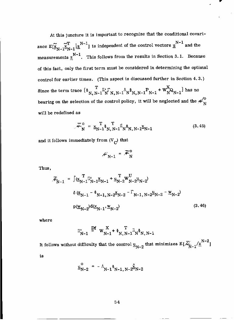
At this juncture it is important to recognize that the conditional covari-
_-_ _ , N-1. N-Iante E[XN_iXN_iIz ] is independent of the control vectors u and the
N-Imeasurements z . This follows from the results in Section 3.i. Because
of this fact, only the first term must be considered in determining the optimal
control for earlier times. (This aspect is discussed further in Section 4.3.)
Since the term trace [_N T_II1EN, N_IAN_N, N_IPN_I + W_NQN_ 1]has no
bearing on the selection of the control policy, it will be neglected and the _N
will be redefined as
and it follows immediately from (V C) that
_J"N- 1 N
Thus,
;(x T [I' x + T U' I_-i N-I-N-I UN-2WN-2P-N-2)
(_N-I - _N-I, N-2XN-2 - FN-I, N-2_N-2 - WN-2)
P(_-N_2) d(-_N_I, WN_2 ) (3.46)
where
It follows without difficulty that the control UN_ 2
is
o _ :_UN_ 2 AN_I_N_I, N-2_N-2
WNX-I + CN,T-IIIN_N, N-I
that minimizes E[_ N_ i/zN-2]_
54

where AN_ I is defined by (3.36) - (3.38). The proof for any k assuming that the
O
"_N-k-2 is (again, retaining only those terms that depend upon the control)
T T_N-k+2 = XN-k+l_N-k÷2, N-k+iIIN-k+2 _N-k+2, N-k+IXN-k+l
is obtained directly from (Vc).
Q.E.D.
This completes the solution of the optimal stochastic control problem for
the linear system (I-L) - (H-L) and the quadratic performance index (IIIc-L) .
By necessity, the discussion has been restricted to the most important aspects
of the problem. The reader is directed to References 40 to 44 for a more
detailed examination of the linear problem.
55

PRECEDTT_G_I _;I]BLANK NOT FILMED.
CHAPTER FOUR
A GENERALIZATION OF THE KALMAN FILTER
In this chapter, the perfurbative Bayesian scheme described in Section
1.3 is applied to the problem of determining an approximation to the a posteriori
density function associated with a nonlinear system. In compliance with the
aforementioned technique, the form of the density must be specified. It shall
be required to be gaussian for all k. This leads to a natural generalization of
the Kalman filter and suggests several interesting conclusions.
The approximation that is described in this chapter represents a generali-
zation of a result obtained by Aoki [33]. Results obtained by other investiga-
tors also indicate that the Kalman filter does not represent the most general
gaussian approximation. This problem has been considered for time-continuous
systems by Bucy [20], Bass et al [21], and Fisher [23]. Jazwinski [45] has
dealt with cases that involve discrete measurement data. His result has the
disadvantage that it does no___treduce to the Kalman filter when the nonlinear
effects are set equal to zero. It is shown in Section 4.2 that the equations
derived here do reduce to Kalman's relations.
The general result is stated in Section 4.1, and an outline of the deriva-
tion is presented. Several interesting conclusions follow from this result, and
these aspects are discussed in Section 4.2. The control of a system described
by a linear plant and nonlinear measurements is discussed in the light of this
approximation, and it is suggested that the Separation Principle is no longer
valid for this system.
57

The filter resulting from this approximation is utilized in Chapters 5
and 7 to determine its behavior relative to linear and other nonlinear filters.
The results that are obtained, particularly those in Chapter 7, suggest that one
must approach the problem of approximating the a posteriori density with
caution because it appears that the estimates provided by this filter are biased.
This undesirable feature is discussed in more detail below. Another gaussian
approximation is discussed in Chapters 6 and 7.
4.1 AN A POSTERIORI GAUSSLAN DENSITY FOR FILTERING OF NONLINEAR
SYSTEMS
Consider a system in which the state _k evolves according to the non-
linear difference equation
where _k is n-dimensional.
with mean and covariance
S[_wj] = 0_ for allj
E[wj_] = QkSkj
Note that no control terms are included in (I-N)
The measurement data -_k are described by
--
where _k is m-dimensional.
mean and covariance
: +
The additive noise -_-k-1
The additive noise -_k
(I-N)
is a gaussian sequence
E [y_] = O for all j
(II-N)
is a gaussian sequence with
58

The sequences{_yk] and [_Wk] are assumedto be independent.
E[_ T] =- 0 for allk,j.
The initial state x"-O
covariance
Also, the x"-O
That is
is taken to be a gaussian random variable with mean and
txl = a
E[_xu_] = M°
is independent of the noise sequences.
The covariance matrices {tL],K {Qk ]' and M shall be assumed to beO
positive-definite in much of the succeeding presentation, but this is not a
severe restriction. If any of these matrices were singular, an appropriate
linear transformation would yield random variables of smaller dimension that
have positive-definite covariance matrices and the derivation would be carried
out in terms of the new variables. Further, the restriction can be seen to be
relaxed in the final relations that are obtained for the estimation policy.
The noise has been assumed to be additive in (I-N) and (H-N) in order to
simplify the densities p(xk/_k_l ) and p Z(_k/Xk ). If non-additive noise were
assumed, it would be necessary to introduce the Jacobians of f-k and _k with
the concomitant complications.
59

The procedure described in Section 1.3 shall be used to approximate the
p(_x_/k). It will be assumedthat nominal valuesa posteriori density function
will permit the conditional density p(__xk/z__k) to beare available that
gaussian for all k. Taylor series expansions of the _-k and _k will be intro-
duced using the nominal values of the state. This procedure leads to a generali-
zation of the results for linear systems (i. e., of the Kalman filter).
Before proceeding further, let us introduce some of the notations that
will appear. Let
8f
Fk Df= (_)=k+l, =
" ' " n
1 naxk evaluated with
with the superscripts denote the component of the vector. The first partial
derivatives of _+1 with respect to _k+l are
Df 3_k+l ,
The derivatives are evaluated with
Df
=
Second partial derivatives are also used.
portent of _k+l and _k+l are denoted as
.thThe second partials of the i com-
6O
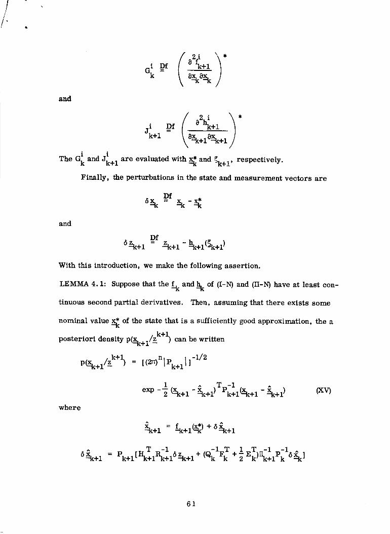
//" .
(2i 1i Df 8fk+l
% -- a%a%
and
The Gk and iJk+l are evaluated with _ and _k+l' respectively.
Finally, the perturbations in the state and measurement vectors are
Df6%-- %-%_
and
Df
With this introduction, we make the following assertion.
LEMMA 4.1: Suppose that the [k and _k of (I-N) and (H-N) have at least con-
tinuous second partial derivatives. Then, assuming that there exists some
nominal value _ of the state that is a sufficiently good approximation, the a
• . k+lposteriori density P_Xk+l/Z ) can be written
p%+/_+_ --I_nIPk+_Ij-_P
where
1 ^ Tp-iexp--_%+1- %_+1) k+1%+1
^ A
_+_ = _+_) +_+_
-_k+l) Ocv)
= p T -i z -i T 1 T -i -i ^
61

At tO
-i FkPkF:)-i T -i -I= - 2 Ek_k+lFkQ kPk+l (Qk +
m
ET--I T R-I- i ik _k+lEk Hk+ 1 k+lllk+l _ l- + - Jk+lYk+l
i=l
the density is gaussian with mean-0
= x*+5£"-O --O --O
and covariance P .0
^ °•>5x = Po[H R z +M a]-'O O ,
m
P = [HTR-IH -ZJi i + _1]-1
o o o o oy ° Mi=1
Most of the quantities appearing in (XV) have already been defined.
ithe Yk+l are components of the vector
Df -i
Zk+l = 1 k+16- +1
andn
.T
Ek Df Z i -i -i
i=l
Df T -i -i[Ik+l = FkQk Fk+Pk
.T1 th -1
The flk is the i row ofO. •"K
However,
As was shown in Section 2.1, the minimum mean-square estimate is
provided by _k+l" Note that Pk+l is a covariance matrix, so it must always
be non-negative definite and preferably should be positive-definite. The man-
ner in which the second order terms enter the defining relation suggests that
Pk+l might lose this sign-definiteness if the magnitude of these terms becomes
too large. This can provide a criteria for judging when the nominal no longer
62

provides a reference that is adequate for the gaussian property to remain
valid.
Proof: In the subsequent pages, only a detailed outline of the proof is given.
The complete derivation is found in Appendix A.
The a priori statistics for x, [Ki] , and [Xi} are gaussian and described
by (3.1) - (3.3). The desired recursion relations are obtained inductively.
• k+l
First, the initial density function p x_/z) is determined, and then p(__Xk+l/Z )
is derived after assuming the gaussian form for p(xk/z_.
p%/x) = kvoxp- % (4.
Expand h in a Taylor series about x* and retain only the quadratic terms in--O --0
6x that appear in _ - h__)TRolZ(_ ° - h__). Then"-0
1 zTR-16 zpz(_/_)) = k exp - 7 [6 - 25zTR-IH 6x
V "O O -'O -'O O O --O
+ 6x_oT[HTR-IHO O O
m
- JoYo ]5-ox]
i=l
(4.2)
where the notation has been defined above. The nature of the approximation of
pz_/Xo) (and, more generally, the pZ__k/Xk))has been found to a criticalcon-
cern in attempting to describe the p_k/Z_. This aspect will be discussed in
Chapter 6.
Substitution of (3.3) and (4.2) into (2.15) yields
1 1 ^p%/z) = ko exp- _ [X(_o- X__o)TP° %- x)] (4.3)
where
= x*+5_--O --0 --O
63

6:_ = [HTR-16z +M-16a]-o Po- o o -o o -
m
Po = [HTR:IHo- Z iiJoyo +M-I -lo ]
i=1
and
Df6a = a -x*
m _ _0
The minimum mean-square estimate of x"-0
• k+lA posteriori density p(_xk+l/Z - )
given the dataz is_ .--O --O
To determine the relations for an arbitrary sampling time, assume at
t k that
1 ^ T -1p(_xk/zk ) = k kexp _[% ] (4.4)- -Kk) Pk _k--Y-_k )
The derivation of p%+l/zk+l)is_ accomplished according to the following steps.
1. Formp%+1/5.
From (3.1) and (l-N), it is clear that
1 TP_k+i/!!k ) = k exp _ [(_k+l - (4.w - - _k+l ) Qk%+l f-k+l )} 5)
Expand f-k+l in a Taylor series and retain only the quadratic terms (and lower
order) in 5 _k in the exponent. This result in combination with (4.4) produces
p (y._+ i/z_ kkkw exp 1- kN k - _ [64+1%16!ik+1 + 6_Pkl6_k
where
T -I Pkl6 _k ]6_k = BktFkQ k 5%+1+
64
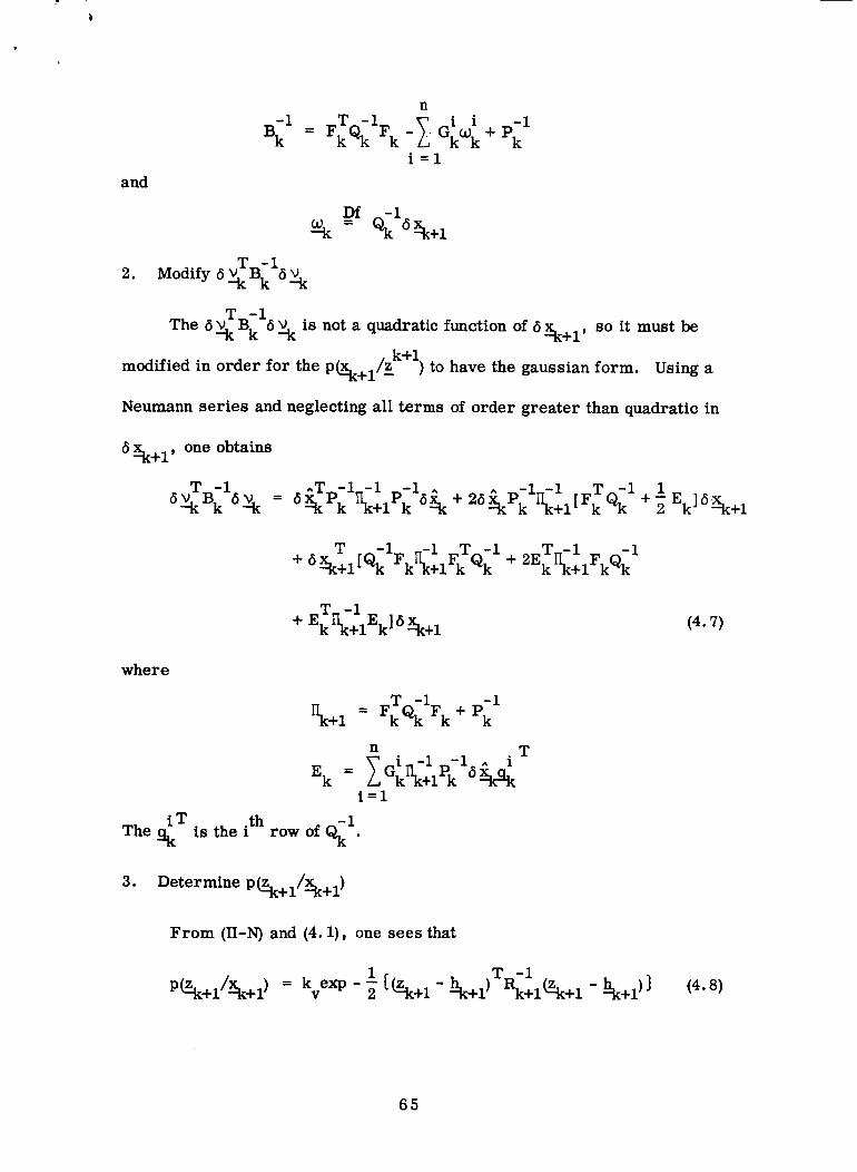
and
n
-1 FT-1 F i i -Bk k% k-I + Pkl= Gk_0 k
i=l
Df -i
-_k = Qk 6_k+1
2. _odify_Bk1_
_Bkl5 is not a quadratic function of 6 _k+l' so it must beThe 6 _k
• /zk+lmodified in order for the pt.xk+1 _ )to have the gaussian form. Using a
Neumann series and neglecting allterms of order greater than quadratic in
5 _tk+ I, one obtains.... -I -i T -i 1
T -_ -_ T -_ T--_F -_+ 5%+1[ % FkRk+lFk Qk + 2EkRk+l kQk
(4.7)
where
The _k is the
-1= FT--IF +Pk
Rk+l k Qk k
n .T
= Gi_-i R-16 ^Zk I kt_ +I k
i=l
-i
row of Qk "
3. Determine PZQ_k+i/[_k+I)
From (H-N) and (4.i), one sees that
p%+/%+1_ = kve_P- _ _%+1- _k+l) k+1%+1(4.S)
65

Expand_k+l
P%+/_k+l)
in a Taylor series and retain only the appropriate terms. Then
=kV
.
that
Form P Z(_k+l/Z_
1 T_-I 6exp-_ [_+iKk+1_k+lJ
m
1 T R-I _ ji i .exp-_{6Y_k:l[Hk+l k+lHk+l _ k+lYk+l 1
i=1
z T -16Xk+ 1 - 26=.k+iRk+iHk+15 Xk+l ] (4.9)
It follows in a straightforward manner from (IV), (4.6), (4.7), and (4.9)
kkkwkv exp 1 {szkTiRk+16 ^ T -1kk+ikNk - _ %÷i - _%÷Pk÷1_k÷1
where 5-k+l
5.
_,+ - Pk _k+iPk ]
and Pk+l shall be defined below.
•k+l
Form p(__+l/Z )
(4.10)
Performing the operations indicated by (IV), the a posteriori density is
found to be given by (XV) thereby completing the proof.
Q.E.D.
4.2 ON THE APPROXIMATION OF NONLINEAR SYSTEMS
Commonly, the analysis of the nonlinear system (I-N) and (H-N) is
approached by introducing linear perturbation theory. This requires the choice
of nominal values _-1 for the state. Then, the linear perturbation equations
are
66

= Fk r -i + (4.11)
where the F k and Hk have been defined in Section 4.1. The choice of the
nominal is made somewhat arbitrarily, and its adequacy is gauged by the sub-
sequent results.
Assuming that (4.11) and (4.12) are accurate representations of the
deviations from the nominal, the problem of estimating _k reduces to the
simpler problem of estimatingSx k. Since this system is linear and the noise
sequences are gaussian, the recursive minimum mean-square estimate of 5_k
is given by the Kalman filter equations of Section 3.1. The result of the pre-
ceding section gives a generalization of this linear approximation, and in so
doing, provides insight into other aspects of the problem, including the choice
of the nominal.
4.2.1 Relation to the Kalman Filter
In this section we shall demonstrate that (XV) reduces to the Kalman case
when the matrices containing the second partial derivatives are identically zero.
Let
i = ji = 0 for all i,jGk k+l
Then, it is true that
The equation for _i_k+l
Ek=- O.
in (XV) reduces to
T -1 - - -= Pk+l[I-Ik+lRk+16z.k+l + QkiFkl]kllPklS_k ]
67
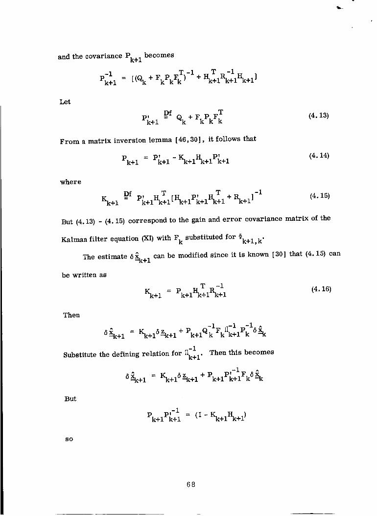
and the covariance Pk+l becomes
-1 = [(% + FkPkF[)-I T -1Pk+l + Hk+iRk+iHk+l ]
Let
p, Df Tk+l = Qk + FkPk F (4.13)
From a matrix inversion lemma [46,30], it follows that
= p' p'Pk+l k+l - Kk+lHk+l k+l (4.14)
where
Kk+l __Drp, _ T , T -i (4.15)k+iHk+l [Hk+iPk+iHk+l + Rk+ I]
But (4.13) - (4.15) correspond to the gain and error covariance matrix of the
Kalman filterequation (El)with Fk substituted for #k+l,k"
The estimate 5_k+l can be modified since itis known [30 ] that (4.15) can
be written as
= p - TR-1Kk+l k+1 +1 k+l (4.16)
Then
6__k+ 1 = Kk+16_k+ 1 + P_ _Q-1F_II-1 p-15:_k+l K k k+l k --k
Substitutethe defining relation for II-I Then this becomesk+l"
I--1 A
6!_k+ 1 = Kk+16_k+l + Pk+lPk+lFk6!! k
But
-1Pk+lP_+l = (I - Kk+lHk+l)
SO
68

A
6%+I = Fk6 % + -Hk+iFk 1
which is the Kalman estimate.
4.2.2 Choice of the Nominal
The values of the state that are chosen as the nominal will obviously play
a key role in determining the validity of the approximation. For many prob-
lems (e. g., space navigation), it is convenient to specify a nominal before the
system is in operation and to then compute many of the quantities required by
the filter off-line. This policy minimizes the amount of computation that must
be performed while the system is in operation. It has been suggested that it is
not always desirable to prespecify the nominal because the quality of the linear
approximation is caused to deteriorate more rapidly° The filter described by
(XV) provides analytical corroboration of this intuitive idea and demonstrates
that the best choice of nominal at each sampling time tk+ 1 is the _k"
In (XV) suppose that the nominal is selected as
with this nominal, it is obvious from
that
5_k - 0.
The estimate (XV) reduces immediately to
-1(4.17)
69

Furthermore, from the definition of Ek, observe that
Ek-- 0.
Therefore,
m
- _ T R-I i i -iPk+l 1 "k+l k+l k+l= + - Jk+lYk+l ] (4.18)
i=1
Certainly (4.17) and (4.18) are simpler in appearance than their counterparts
i from the plant hasin (XV). In fact, one notices that the second order term G k
disappeared entirely. The error covariance matrix Pk+l contains the second
order measurement effects jik+l' and these terms cause the Pk+l to depend
upon the measurement data. This is in sharp contrast with the Kalman filter
in which the error covariance matrix and, therefore, the gain can be computed
off-line.
With this choice of nominal, the minimum mean-square estimate is seen
to be
=f ^ +
is defined by (4.16) and
=
where Kk+ 1
- hk+l _(_k+l)] (4.19)
in (4.18) can be written in a form that is more computationally
L Df , -1 T -1 -1Pk+1 = [(Pk+l) + I'Ik+1Rk'_lI'Ik+1]
The Pk+l
attractive. Let
By a matrix inversion lemma, this is equal to
+R-I -i p,k+l ) Hk+l k+l
p L _ p, T p, Tk+l = Pl_+l k+iHl{+l(Hk+l k+lHk+l
70

With this definition, (4.18) becomes
m
= pL ji i pL -iPk+l k+l[ I- ( _ k+lYk+l) k+l]
i=l
When the second order terms are not present, this becomes
=pLPk+l k+l
and we note that P Lk+l is the error covariance matrix of the Kalman filter.
4.2.3 Conclusions
The preceding development has produced several interesting results.
1) Linearization of the nonlinear plant and measurement equations
about some nominal does no.__tprovide the most general form for
the mean and covariance of a gaussian conditional probability
density function P(Xk/Z__.
2) Expansion of the nonlinear plant and measurement equations about
arbitrary nominal values subject to the constraint that the density
P(Xk/Z_ must be gausstan produces mean and covariance that
depend upon the second order terms of the expansions. In con-
trast with the Kalman filter, the covariance depends upon the
measurement data.
3) If for each k the plant equation _-k is expanded about the conditional
mean _k-l' all second order terms from the plant equation are
eliminated in the relation for _k" The covariance still depends
upon the measurement data and contains second order terms of
the measurement equation.
71

4) The defining relation for the conditional variance Pk+l contains
negative terms that could destroy the positive- (or non-negative-)
definiteness property required for this matrix. If such a situation
were to arise, it would suggest that the nominal values were no
longer an adequate reference and would suggest that a nongaussian
conditional density function is required.
The disadvantages inherent in these results arise primarily through the
increased number of computations that must be performed on-line. That is, if
s,
the minimum mean-square estimate provided by _k+l in (4.20) is used, the
error covariance matrix must be computed during the operation of the system
described by (I-N) and (II-N). In the Kalman filter, this matrix does not depend
upon the measurements, so it can be computed in advance if the nominal has
been specified. Also, if the estimate is treated as the nominal, it is necessary
to compute all system matrices on-line since the Fk, Hk, and jik+l are all
computed using the nominal values. Thus, the computational load is greatly
increased if this formulation is to be implemented. Additional remarks regard-
ing the nonlinear filter of Section 4.1 are found in Chapters 5 and 7.
4.3 ON THE CONTROL OF A LINEAR PLANT USING NONLINEAR
MEASUREMENT DATA
In this section, no formal results are to be exhibited. Rather, the filter
derived in Section 4.1 will be utilized to suggest that the Separation Principle
of Section 3.2 cannot be extended to the situation in which the plant is given by
: tk, k-lX'--1--K + Fk, k-lU'--1--K + -_-k- 1 (I-L)
72
and the measurements are described by
(II-1_
As in Chapter 3, consider the problem of establishing the control policy
for the system (I-L) - (II-N) that minimizes the quadratic performance index
(IIIc-L) under the constraint on _k that the a posteriori density remain gaussian
for all k.
For the last stage, the function _ is easily seen to be (re: equation
3.40)
T= xNTI_N,N_IWX N N,N_IXN_I
T T
+ 2 XN_I_N, N_IW_N, N_IUN_ I
+ T . U TUN_I(WN_ I + FN, N_IWXiN, N_I)UN_ l+trace [W_NQN_I]
The control that minimizes E[_.N/zN-1]_ is
(4.2i)
O
UN_ 1 = - AN_N,N_I_N_ I (4.22)
where AN is defined by (3.42). In this case the estimate is not given by the
N-2Kalman filter equations. It follows from Section 4.1 and the fact that the u
is known that
_N-I = _N-I,N-2_N-2 + KN-I(_N-I - HN-I_N-I,N-2_N-2 )
where
+ (I- KN_IHN_I)FN_I, N_2_N_2
T -i
KN_ I = PN_IHN_IRN_I
m
, ,-= - HN_IRN_IHN_I - I JN_IYN_ I
i=1
(4.23)
73

pt = TN-I _N-I, N-2PN-2_N-I, N-2 + QN-I
Thus, the Separation Principle is valid for a_single-stage problem.
Unfortunately, it does not appear to be possible to extend this to multi-stage
problems. We shall consider a two-stage problem and indicate the reason for
the added difficulty.
problem.
t _ oAs in (3.43) of Section 3.2, he_- N can be written as
-o T T
N = XN-I_N, N-I[IN_N,N-IX-N-I
From/_'N-I
No attempt will be made to derive the control law for this
+xT_ T rl'--N-I N, N-I _N, N-IAN_N, N-IXN-I
+ trace (W_NQN_I)
according to (Vc)
= _ZN6 _-N-1 -hN-1)P(Y-N-I)d(Y-N-I'ZN- 1)
= X_N_I_N, N_IHN_N, N_lXN_I + trace ( QN_I)
+ _N, N-1H_{VN, N-IAN_N, N-lXN-I
(4.24)
6 _N-I - hN-I)P(Y-N-I)d(Y-N-lZN-I) (4.25)
In contrast with the linear filter, the term involving XN_ I does contribute
to the control. To verify this, we shall perform the integration of (4.25) with
respect to ZN_ 1. Then, as indicated in the formation of_N_l in (Vc), one
must integrate with respect to XN_ 1. After these two integrations are performed,
the error can be written as
74

XN_1 = _N_I,N_2XN_2 + KN_I[hN_1 + VN_1 - HN_1
(_N-I, N-2_N-2 + FN-I, N-2UN-2 )] - WN-2
As has been indicated in Section (4.1), the hN is approximately
hN-1 = HN- lXN -1 + v2h
(4.26)
(4.27)
where
V 2hDf
T 1XN-?N-IXN-I
i
T m
X--N_IJN_IXN_ I
Introducing (4.27) into (4.26), one obtains
N N
XN_ I = _N_I,N_2_N_2+KN_I[HN_IXN_I + v2h-+VN_I
- HN_I(_N_I,N_2_N_ 2 + FN_I, N_2_N_2)] - EN_ 2
But XN_ I is described by (I-L) so thisbecomes
XN_ I = (I - KN_IHN_I)(_N_I,N_2_N_ 2 - Ek_l ) + KN_IV 2h+KN_IZN_I
At this juncture, let us recall thatin the linear problem, the V 2h would
be identicallyzero and the gain KN_ I is independent of the measurements.
Thus, as was stated in Chapter 3, the term involving XN_ I does not contribute
to the control policy. It is this fact that permits the proof of the Separation
Principle for linear systems. It is clear from (4.15) and (I(%/")that KN_ 1
depends upon the measurement data ZN_ 1 and must, therefore, contain the
75

control UN_ 2. Furthermore, the v2h depends upon XN_l, so from (I-L), it
2h_must be true that _7 must contain UN_ 2.
2 _"The V h and the KN_ 1 do not allow the term involving XN_ 1 in (4.25) to
be neglected in determining the control policy. This was necessary in estab-
lishing the Separation Principle in Section 3.2. Of course, if one were to con-
tinue the derivation, it might be found that the control is unaffected by these
terms, but this would be surprising.
76

CHAPTER FIVE
FILTERING FOR NAVIGATION OF A SPACECRAFT
Several of the results of Chapters 3 and 4 are applied to the problem of
estimating the state of a spacecraft. The linear filter of Chapter 3 is utilized
for the greater part of the study contained in this chapter. In many cases,
linear perturbation theory is found to adequately describe the physical system,
so one would expect the linear filter to perform "satisfactorily". Occasions do
arise, however, when the nonlinear effects seriously affect and sometimes
even destroy the validity of the output of the linear filter. It is the intent in
this chapter to illustrate both of these situations. Then, several techniques
are investigated which allow the range of applicability of linear theory to be
considerably extended. Finally, the nonlinear filter of Chapter 4 is applied to
the problem to illustrate the effect of including nonlinear terms. These results,
unfortunately, are of a somewhat disappointing nature.
The basic problem and the mathematical model are discussed in Section
5.1. The numerical results obtained from the digital computer simulation of
the problem are presented in Section 5.2. The conclusions that can be drawn
from these results are presented in Section 5.3.
5.1 THE SPACE NAVIGATION PROBLEM
The objective in this chapter is to consider the applicability of perturba-
tive techniques to a significant nonlinear problem. In particular, the problem
of estimating the position and velocity (i. e., the state) of a spacecraft moving
in a nearly circular orbit about the Earth is studied. The estimates are to be
based upon the measurements provided by a horizon sensor aboardthe craft.
77
Several different estimation policies are utilized, although the linear
filter described by (XI) provides the basic configuration. The policies are
listed and described below. Before discussing them, the basic mathematical
model shall be presented. A more detailed discussion can be found in
Appendix B.
5.1.1 The Mathematical Model
For this study, the Earth shall be assumed to be spherical with radius r o
and to have a spherical gravity potential U described by
U -R
The _ is a constant equal to the product of the mass of the Earth and the uni-
versal gravitational constant. Let R be the distance from the center of the
Earth to the spacecraft.
A coordinate system is defined to be a nonrotating cartesian system with
origin at the center of the Earth. The coordinate axes shall be denoted by X, Y,
Z. The motion shall be assumed to occur, primarily, in the X-Y plane. In
this system, the equations of motion for the spacecraft are known to be
= - R (5.i)-- R 3 --
In order to use state vector notation, (5.1) must be reduced to a first order
differential equation. This is accomplished by defining the state x to be the
six-dimensional vector formed from the components of the position R and
velocity _ vectors.
78

X
J
v
Df
X
Y
Z
X1
X 2
X 3
X 4
X 5
X 6w
Then, the state is seen to evolve according to
/tt V
i
i
v -R- 3!
IXf_(_x) (5.2)
For this system we shall assume that the plant does no___tcontain any noise, so
(5.2) provides the specific form for the plant equation (I) to be considered in
this example.
The position and velocity of the spacecraft are to be estimated using the
angular measurements from a horizon sensor. This instrument is assumed
to measure:
(1) the direction of the local vertical relative to the X-axis of the
coordinate system• The direction is specified by the two angles
and 5, where _ is the angle between the X-Y plane and the line
of sight and 5 is the angle between the X-axis and the projection
of the line of sight onto the X-Y plane.
(2) the subtended Earth angle ft. The fl is defined as the angle between
the line of sight to the edge of the planet and the local vertical•
79

These angles are depicted in Figure B-1 of Appendix B and are given by
-1 X3= - sin
R
-i6 = sin
X 2
2 .2,1/2(X 1 + A2)
r-1 o
= sin R
(5.3)
Let
6 (5.4)
Assume the measurements contain an additive, gaussian white noise sequence.
Then, (5.4) completes the definition of the measurement equation (II-N) for
this example.
The nonlinear equations (5.2) and (5.4) must be expanded in Taylor series
relative to some choice of nominal values for the state. To apply the Kalman
filter of Chapter 3, the system must be reduced to a linear model, whereas
second order terms are required for the filter of Chapter 4. Assume that the
required nominal x* exists and expand (5.2) and (5.3) in a Taylor series. In
this chapter the plant equation will always be assumed to be linear, so one gets
6x_ = F6x (5.5)
where F is the matrix containing the partial derivatives of f__with respect to
x. Let
Df6X = X-X*
8O

The solution of (5.5) is known to have the form [3]
5Kk = }k,k_15Kk_1
is the state transition matrix and is the solution ofwhere _k, k-1
with initial condition
_=F_
(5.6)
(to, to) = I
For the dynamical system (5.2), it is possible to obtain I in a closed form [55].
The solution is presented in Appendix B. Equation (5.6) will serve as the plant
equation for the perturbed state. Note again that no noise appears in this
relation.
The first and second order partial derivatives of a, 5, and fl are formed
in a straightforward manner. They are presented in Appendix B. In many
instances, the partial derivatives are very difficult to determine analytically
because of the complicated nature of the equations. Wengert [47] has sug-
gested a procedure for determining these derivatives in terms of elementary
functions that seems to be quite reasonable. Wilkins [48] applied this approach
to a complicated system and concluded that the method was very satisfactory.
We mention this work because it appears to be a necessary consideration for
the development of a practical nonlinear perturbation theory.
5.1.2 The Estimation Policies
Most of the results presented in the next section are based upon the
linear filter described by Lemma 3.1 of Chapter 3. Five different policies are
examined using the linear filter. Two additional policies are investigated using
81
the nonlinear filter described by Lemma 4.1 of Chapter 4. Each of the policies
is discussed in the detail deemed necessary in the succeeding paragraphs.
(L-l) Linear filter with a prespecified nominal
The linearization is performed relative to a circular orbit at a
100 n. mile altitude. This nominal is used throughout the flight
and the filter equations (XI) are utilized.
(L-2) Linear filter using _k-1 as the nominal state at each tk
It was observed in Section 4.2 that the most appropriate choice
A
of nominal at each sampling time tk is the estimate _k-l" Thus,
at every sampling time, the nominal is selected to be
The linearization is accomplished relative to this nominal, and (XI)
is again utilized. In this case, observe that
6_k_l = 0
after the change of nominal has been completed. This procedure
shall be referred to as rectification.
Rectification has a disadvantage in that all of the system matrices
(i. e., _k,k-l' Hk' etc.) must be recomputed at each sampling time.
If a prespecified nominal is used, the system can be computed and
stored prior to the actual realization of the system.
error covariance matrix Pk and the gain matrix Kk
computed. This results in a considerable reduction of on-line
computation. On the other hand, the additional on-line computation
In fact, the
can also be pre-
82

(L-3)
does not represent a significant restriction in many cases, so
rectification provides a very sensible means of extending linear
theory.
Two means of extending the linear theory without resorting to orbit
rectification are suggested. The first can be applied to systems
containing plant noise as well as measurement noise.
policy is restricted to systems with noise-free plants.
regarding these policies follow immediately.
Modified Observation Matrix H k
The approach used in establishing this policy shall be discussed in
somewhat greater detail in Chapter 6. For the moment, consider
the measurements to be described by (II-N).
-- +
Assuming a nominal, expand _k in a Taylor series and retain the
thfirst and second order terms. The i component is given by
z - Ni
j =lOX k j =1./=1
As has been noted, the ith row of the observation matrix H k is
partial derivatives are evaluated with the nominal values _. )
The second
More details
83

In approximating _k by HkS_k, it is clear that the secondorder
(andhigher) terms are neglected. But this can be circumvented
to a certain extent through the following artifice.
predicted estimate of 5Y_k (i. e., E [5 Xk/5 zk-1]}.
and the plant equations.^
depends upon 6 _k-1
then
Consider the
This estimate
If the plant is linear,
5_k' = _k,k_lS_k_l
As long as the error in this estimate is small compared to the
estimate itself, (5.7) can be approximated by
A
In (5.8), the 5 _' has been substituted for the state perturba-
tions 5 _k" The relationship between the measurements and the
state is linear, but it contains the second order partial derivatives.
The elements of the observation matrix are redefined as
(5.9).. " n 82h_
This modified observation matrix is used in conjunction with the
linear filter and prespecified nominal described in Case (L-l},
and constitutes the third policy. Note that if rectification is
utilized, the predicted estimate is identically zero and Hk is
reduced to the first order terms.
84

(L-4) Re-estimation of the initial state
Since there is no noise in the plant, a smoothed estimate of the
initial state deviation can be easily determined from 6 _k" In
particular, assuming that
6_k = _k,o6_o
it follows that
^
6X/k
(5.10)
where 5 _k is the estimate provided by the linear filter equations.
A
Using the smoothed estimate 6 _o/k and the true equations of motion,
one can determine an estimate of the current deviation that elimi-
nates the errors that accrue through the linear approximation of the
A
plant behavior. To determine this estimate, let Xo/kbe the estimate
of the initial state
^ = x*+5_Xo/k -o -o/k
Then, the estimate of the current state can be computed as
The _k needs to be computed only when it is actually required
(e. g., when a guidance maneuver is to be introduced that is based
u_o__ or_ _ _ _or*_ ,o_o_t_o.o_,_a__ pre-
specified.
85

(L-5) Rectification using a smoothed estimate
It is possible at each sampling time t k to form a smoothed estimate
6 _k-1/k using (3-28). One would expect that this estimate would
A
generally be superior to 6 _k-1 since it is based upon more data.
Then, let the nominal state be selected as
A
= +
-- A
The old nominal __1 ) is computed from 6_k_1 as discussed in
Case (L-2). The smoothed estimate is only used to modify the
A
nominal so the estimatc of the perturbation 6 r_k_ 1 used in comput-
ing 6 _k is set equal to -6 _k-1/k" This policy essentially doubles
the computational requirements required in Case (L-2).
This completes the definition of the estimation policies that are investigated
using the linear filter. Cases (L-l) and (L-2) are repeated using the nonlinear
filter described in Chapter 4.
(N-l) Nonlinear filter with a prespecified nominal
^
(N-2) Nonlinear filter using Xk_ 1 as the nominal state at each tk
These policies describe the basic nature of the numerical investigation.
These cases were investigated for a variety of sampling intervals, instrument
accuracies, deviations in initial conditions, and random noise sequences. The
data that are presented in Section 4.2 are representative of the type of results
that were obtained. In order to most clearly demonstrate the character of the
results, a minimum amount of data has been included.
86

Two types of data are presented. Certainly, the error covariance matrix
Pk should describe the effectiveness of the filtering procedure if the model is
accurate. Since we are approximating a nonlinear system, the Pk does not
always reflect the covariance of the error in the estimate, so a Monte Carlo [61]
simulation (i. e., a random number generator is used to simulate the noise in
the measurements) is performed to obtain samples of the actual error in the
estimate. These errors are compared with the semi-axes of the position and
velocity error ellipsoids [ 10,30] in an effort to determine if the error covari-
ance matrix is a valid measure of the errors.
5.2 NUMERICAL RESULTS
The trajectory that is examined is approximately a circular orbit at
100 n. miles altitude. The constants assumed for the Earth model are [63]
1016= 1.4076539 x ft31sec2/
r = 20,925,738.0 ft.O
The initial conditions for the nominal (i. e., before any measurements) are
designed to give a 100 n. mile circular orbit based on these constants.
R
m 21533391i 010 ; V = 25,567. 728
0 0
The initial conditions for the actual trajectory are unknown, but the deviation
from the nominal is assumed to belong to a gaussian ensemble with mean zero
and prescribed covariance matrix M . The M is assumed to be diagonal with0 O
the general form
87
Mo
where 2 and a 2 are the variances of the position and velocity deviations,p v
respectively. The a 2 and cr2 represent parameters that can be varied for thep v
study and the values that are used will be stated below. These statistics are
used in conjunction with a gaussian random number generator to establish the
initial conditions for the actual trajectory.
The noise corrupting the measurements is also assumed to be gaussian
and has mean zero and covariance matrix R k. The R k is treated as having the
form
R k
2
I °1S
a __°and a 2 represent the variance of the noise in the local verticalwhere theL S
2 2and subtended angles, respectively. Frequently it will be true that o"L = O"s.
The values for these constants will be stated below.
The time interval between measurements provides another parameter for
the study. Several different intervals were considered, but only results relat-
ing to a sampling interval of 10 minutes will be presented. Since the period of
the orbit is approximately 90 minutes, this sampling interval results in meas-
urement data being available at every 40 degrees of subtended arc. The other
intervals that were investigated did not measurably change the conclusions
88

suggested by this sample rate. It should be noted that Meditch [49] has shown
that the system is not observable if measurement data are available only at
intervals of 180 degrees of subtended arc.
5.2.1 When Linear Theory is Valid
The Kalman filter has been applied [49-53] to the problem of estimating
the state of a spacecraft for a variety of missions and has, in general, proved
to give satisfactory results. Mendelsohn [54] has discussed a case in which it
has not given satisfactory results, however. Many of these studies have dealt
entirely with the error covariance matrix Pk and have not involved any Monte
Carlo simulation. Such a procedure is entirely justified if the system were
actually linear. But since a nonlinear system is being approximated by a
linear system, the validity of Pk as a measure of the response of the filter
depends heavily upon the accuracy of the approximation. In this paragraph, we
consider a case in which the linear system (5.6) apparently provides a good
approximation to the behavior of the actual trajectory relative to the pre-
specified nominal.
For the remainder of this paragraph, let
2o" = (5,000 ft) 2
P2
o" = (5 ft/sec)2-V
The initial conditions for the actual trajectory are selected from an ensemble
described by these statistics. For the data in Table 5.1, the initial deviations
are
89

- -223961824192
X(to) - x*(to) = -3.9
3.5
-4.0
At any time tk, the deviation should be described approximately by
-%-1 o% -
if (5.6)is adequate. The error in X-component of position and of velocity are
depicted in Figure 5.1 for five orbital revolutions for one particular set of
initialconditions. This trajectory appears to be representative for the group
that were simulated.
It is clear from Figure 5.1 that the error is oscillatory and has an in-
creasing amplitude. In this case the errors do not appear to be significant,
so one would expect that linear theory is adequate. To see that this intuitive
idea is true, consider the following case.
2 2 degrees) 2(;L = (_s = (0.I
Sampling interval = i0 minutes
All of the estimation policies described in Section 5.i.2 were applied to
this configuration. Results for Cases (L-l), (L-2), (N-l) and (N-2) are con-
rained in Table 5. l(a). Cases (L-3), (L-4), and (L-5) are described by
Table 5. l(b). Only two revolutions are studied for Case (L-5) because of the
number of computations that are involved.
90

q.I
0 0
0 4
\i
bI
"_ , / <ooo _ ', / ,
t
__'_ _ ,
t
!
NI
0Ir
° im u _
I ,I '
!
l <_I
' It It
, I d
I
I I
I
I 'I !t
,,, _ i /
", I /
• Io
-_ d
/
°//
!
_ 0
4
I I I0 0 0 0
I0
!
IIf
/ °
•[_0I x scl_ 'X 9 ~ ao.z.z_ _4_.oOIaAX__OI x _ 'X 9 ~ .zo.z.z_ uo_.;._socIXuol_xo._dd V .z_ou]q u3 zo.za_
IO
c4!
Ic_
!
O
oI
elO
&
_De_
t_O
t_
g
91

The results in Table 5.1 verify that the linear model is an excellent
approximation. First, observe that the axes* of the error ellipsoids provide an
accurate measure of the error in the estimate. Second, it is clear that the
results are essentially the same for every filter configuration. As a precursor
of things to come, it can be seen that rectification of the nominal does result
in a smaller actual error in many cases, particularly for the last two orbital
revolutions. The error covariance matrix is unaffected, however.
5.2.2 Orbit Rectification to the Rescue
In this paragraph a trajectory is considered for which linear theory
proves to be totally inadequate for the description of the state perturbation.
For this case, the statistics of the initial perturbation are taken to be
a = 50,000 ft.P
a = 50 ft/sec.v
Several different sets of initial perturbations were studied. In the results
below, these conditions were
40058
75488
35676X(to) - x*(to) = -29.8
-125.4
3.5
In Figure 5.2 the error in the linear approximation in the X and X compo-
nents is depicted. Note that on the scale used, the errors in Figure 5.1 could
not be distinguished from the axis of abscissas. From the magnitude of these
The direction of the axis is not exactly in the direction of the coordinate axes
so the magnitudes are listed according to the coordinate axis that is most
closely aligned.
92

Time Component
(L-l)
TABLE 5. l(a)
Filter Response when the Perturbations are Linear
G =5000ft;G=5 fpsP v
CrL = _Y = 0.1 degrees
Prespeclfied Nominal
5400 X, ft -5639Y, ft 16082
Z,ft 4108
X, fps -20.7
Y. ,fps 0.8
Z,fps -6.1
10800 X, ft -4573
Y,ft 3016
Z,ft 2075
X, fps -4.3
Y, fps 3.4
_., fps -7.5
16200 X, ft 1457
Y, ft -9920
Z, ft 1899
X, fps I0.0
Y, fps 7.4
7., fps -6.8
21600 X, ft -1696
Y, ft 2258
Z,ft 497
_,fps -1.0_', fps -0.2
Z,fps -7.3
27000 X, ft -3442
Y,ft 3800
Z, ft 1392
_:, fps -3.3
Y, fps -2.0
7-, fps -7.7
Error in
Estimate
Axes of Error
Ellipsoids
(N-i) (L-i) (N-I)
-5639 2468 2467
16069 16428 16435
4108 4798 4798
-20.7 18.7 18.7
0.8 2.9 2.9
-6.1 4.9 4.9
-4566 2078 2076
2999 14645 14658
2074 4599 4599
-4.2 16.6 16.6
3.4 2.4 2.5
-7.5 4.8 4.8
1463 1833 1833
-9934 12735 12734
1899 4405 4405
10.0 14.4 14.4
7.4 2.2 2.2
-6.8 4.7 4.7
-1695 1661 1660
2251 11322 11316
497 4218 4219
-1.0 12. S 12.8
-0.2 2.0 2.0
-7.3 4.7 4.7
-3445 1530 1530
3801 10262 10246
1393 4042 4043
-3.3 11.6 11.6
-2.0 1.8 1.8
-7.7 4.7 4.6
Rectification
Error in
Estimate
(L-2) (L-2)
-5608 -5605
16071 16044
4107 4107
-20.7 -20.7
0.8 0.8
-6.1 -6. i
-4516 -4505
2896 2858
2073 2O72
-4.1 -4.1
3.5 3.5
-7.5 -7.5
1565 1580
-10056 -10090
1898 1898
10.2 10.2
7.5 7.5
-6.8 -6.8
-1187 -1180
1625 1618
496 496
-0.2 -0.2
0.3 0.3
-7.3 -7.3
-2603 -2559
3000 2995
1397 1392
-2.3 -2.3
-1.1 -1.1
-7.7 -7.7
Axes of Error
Ellipsoids
(L-2) (N-2)
2478 2478
16433 16446
4798 4798
18.7 18.7
2.9 2.9
4.9 4.9
2100 2098
14638 14650
4599 4600
16.6 16.6
2.5 2.5
4.8 4.8
1846 1845
12598 12600
4406 4406
14.3 14.3
2.2 2.2
4.7 4.7
1665 1665
11214 11211
4219 4220
12.7 12.7
2.0 2.0
4.7 4.7
1535 1535
10346 10346
4044 4044
11.7 11.7
1.8 1.8
4.7 4.7
93

TABLE 5. l(b)
Filter Response when the Perturbations are Linear
% --5000 % --5a L = as = 0.1 degree
Time
54OO
10800
16200
21600
27000
Component
X, ft
Y, ft
Z, ft
X, fps
_', fps
_, fps
X, ft
Y, ft
Z, ft
X., fps
.Y, _sZ, fps
X, ft
Y, ft
Z, ft
X, fps
Y, fps
7., fps
X, ft
Y, ft
Z, ft
"X, fpsY, fps
Z, fps
X, ft
Y, ft
.z, ftX, fps
%', fps
_, _ps
Prespecified Nominal
Error in Estimate
(L-3)
-5634
16062
4109
-20.7
0.8
-6.1
-4576
3019
2075
-4.3
3.4
-7.5
1461
-9943
1899
i0.0
7.4
-6.8
-1679
2220
498
-1.0
-0.1
-7.3
-3354
3675
1392
-3.2
-1.9
-7.7
Initial I CurrentState State
(L-4)
-3438 -5623
4281 16087
4734 4110
i. 8 -20.8
3.3 0.7
-5.4 -6.1
-3860 -4558
5165 3015
3605 2076
2.1 -4.3
4.7 3.4
-6.5 -7.5
-2296 1467
4628 -9905
2917 1900
1.5 10.0
3.1 7.4
-5.4 -6.8
-1229 -1656
5587 2252
3474 499
3.0 -1.0
1.5 -0.2
-6.1 -7.3
-1418 -3433
5499 3806
3397 1396
2.8 -3.3
1.7 -2.0
-5. I -7.7
Axes
of
Error Ellipsoid
(L-3) (L-4)
2468 2468
16422 16428
4798 4798
18.7 18.7
2.9 2.9
4.9 4.9
2079 2078
14635 14645
4599 4599
16.6 16.6
2.5 2.4
4.8 4.8
1834 1833
12728 12735
4405 4405
14.4 14.4
2.2 2.2
4.7 4.7
Rectification
Error Axes
in of Error
Estimate Ellipsoid
(L-S) (L-5)
-5585 2468
16072 16432
4108 4799
-20.7 18.7
0.7 2.9
-6.1 4.9
-4485 2090
2852 14629
2072 4600
-4.0 16.6
3.5 2.5
-7.5 4.8
No
Data
1661 1661
11316 11322
4218 4218
12.8 12.8
2.0 2.0
4.7 4.7
No
Data
1531 1530
10256 10262
4042 4042
11.6 11.6
1.8 1.8
4.6 4.7
No
Data
94

errors, one would suspect that a linear estimation theory could not provide
satisfactory results. As shall be shown, this suspicion is entirely valid for
the case in which the original nominal is retained throughout the duration of
the flight. However, rectification of the nominal provides a striking improve-
Once again, consider the followingment in the accuracy of the estimates.
cases
2 2 degrees)2a L = o" = (0.1S
Sampling interval = 10 minutes
Results for cases (L-l), (L-2), (N-l), (N-2) are stated in Table 5.2(a).
It is interesting to examine these data in more detail. First, the error in the
estimate for Case (L-l) becomes intolerable and at no time does the error
ellipsoid describe the error. This disparity is a manifestation of the nonlinear
effects upon the estimated procedure. The error in the estimate during the
second and third orbits has a remarkable correlation with the error in the
For example, the error in the linear approximation oflinear approximation.
16200 seconds is
[x(16,200) - x*(16,200)] - _(16,200, 0)5_. ° =
-259,423
-196,697
-2,262
226.6
-304.1
-6.5
Comparing this with the error in the estimate given in Table 5.2(a), one
observes that the error can be attributed almost entirely to the linear approxi-
mation error. This is important when considering the effects of the estimation
policy (L-4).
95
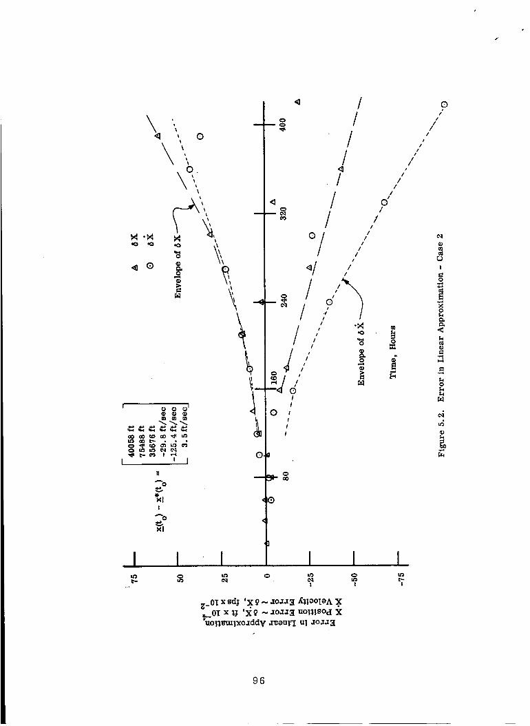
I
O.
60 6O
I
m _ m
I ' I
II
!
A 0
0m n _
0
°/
o/
I
/
/
I
#
Q.
/////
/ !
o'/
!I
I
II
I
/
/
/I
/I
l
m
0
I I I I,, |
0u_!
z_OI x sd_ 'X 9 -- zo_ _!_oIoA .X_OI x _J 'X 9 "_ -_o_z_uo1_.sod Xuol%_'mIxo._dd V z_out'I el ._o_._
0/
/t
//
/I
i /
//
/P
/
I
2
0
e_
.=.
0
M
e_
!
96

I
When the nonlinear filter (i. e., Case (N-l)) is used, an improvement in
the estimate is obtained, particularly during the first orbit. It is apparent that
the general behavior of the filter is not greatly affected and that it is the non-
linearities arising in the dynamics that are completely dominant. Again, the
error covariance matrix does not provide a valid measure of the actual error
in the estimate.
The most significant result appears when examining the effect of rectify-
ing the nominal at each sampling time. For this case, the error in the estimate
is greatly reduced compared with Cases (L-l) and (N-l) and does, in fact,
correspond with the errors predicted by the error covariance matrix. It is
also seen that the error covariance matrix does not appear to be significantly
different from the values obtained for the preceding cases.
The introduction of the nonlinear filter has an unexpected effect upon the
estimate judging by the tabulated data. In almost every instance, in the table,
the error in the estimate is larger although the error covariance matrix is not
affected to any great extent. These results suggest a problem that is consid-
ered in more detail in Chapter 7. However, the tabulated data are somewhat
misleading. For example, an examination of the error in the estimate of the
X component of position for the first ten observations indicates that the non-
linear filter provides a more accurate estimate at about half of the observation
times (six out of ten). This is typical of the response that is observed for all
components of the state vector and leads one to conclude that the nonlinear
term does not provide any appreciable benefit.
97

TABLE 5.2(a)
Filter Response when a Prespeeifled Nominal is Inadequate
a =50,000ft;a =50 fpsp v
a L = a s = 0.1 degree
Time Component
5400 X, ft
Y, ft
Z,ftX, fps
_,fps7., fps
10800 X,ft
Y, ft
Z,ft
_:,_ps_',fpsZ,fps
16200 X, ft
Y,ft
Z,ft
X,fps
Y,fps
Z,fps
21600 X, ft
Y,ft
Z,ft
X, fps_r, fps
Z,fps
27000 X, ft
Y,ft
Z,ft
:_, fps
Y,fps
z,_ps
Prespecified Nominal
Error in Axes of Error
Estimate Ellipsoids
(L-l) (N-l)
-36783 -3456!
-52744 -38406
10599 9398
59.9 50.8
-23.7 -30. c
-24.8 -24.
-137029 -13632£
-93000 -85475
18163 _ 16819
106.9 103.4
-123.2 -127.8
-19.6 -19.2
-275523 -275099
-194631 -188665
8883 8553
228.5 226.4
-284.2 -288.3
-13.6 -14. i
-7. xl06 -6. xl06
11. xl06 i0. xl08
4871 5401
-12653 -11391
-8068 -7767
-14.5 -14.9
-11.x106 -11. x106
14. xl06 14. xl06
4998 5300
-16318 -15027
-14123 -13717
-7.2 -8.4
Rectification
Error in
Estimate
(L-l) (N-l) (L-2) (N-2)
4352 4418 6028 7420
18118 18492 -1898 -3176
16562 15771 10499 10597
20.1 20.2 3.9 7.0
4.7 4.9 -4.8 -5.2
19.6 18.7 -23.4 -23.5
2852 2941 2078 2742
15504 15550 -3730 -4276
12034 11425 18521 18615
17.5 17.4 2.1 3.6
3.3 3.4 0.5 0.6
14.4 13.7 -17.8 -17.8
2271 2356 10845 11244
13620 13620 -14723 -14884
9915 9410 9490 9517
15.5 15.2 16.5 17.2
2.6 2.7 8.9 9.1
11.9 11.4 -11.3 -11.4
1946 2061 7128 7348
12210 11564 -8310 -8281
8625 8188 6108 6110
13.9 13.2 8.8 9.3
2.3 2.4 9.1 9.0
10.4 9.9 -11.7 -11.7
1732 1861 -3567 -3357
11131 10385 987 1055
7736 7339 7067 7055
12.7 11.9 -3.3 -3.0
2.0 2.2 -1.7 -1.6
9.3 8.9 -4.1 -4.1
Axes of Error
Ellipsoids
(L-2) (N-2)
4038 4034
17306 17284
16507 16603
19.5 19.5
4.2 4.2
19.5 19.5
2528 2528
15099 15113
11991 12013
17.2 17.2
2.8 2.8
14.4 14.4
1989 1987
13264 13280
9873 9890
15.1 15.1
2.3 2.3
11.9 11.9
1700 11983
11961 1699
8588 8600
13.7 13.7
2.0 2.0
10.4 10.4
11138 11142
1518 1519
7709 7704
1.8 1.8
12.8 12.8
9.4 9.4
98

Time
§400
10800
16200
21600
27000
TABLE 5.2(b)
Filter Response when a Prespeclfled Nominal is Inadequate
=50,000ft;_ =50 fpsp v
_L = _s = 0. i degree
Component
X, ftY, ft
z, ftX, fps_, fps_., fps
X, R
Y, ft
z, ftX, fps_', fpsi, fps
X, ft
Y, ft
z, ftx,_.Y,fp8Z, fps
X, ft
Y, ft
z,RX, fps_, fpsi, fps
X, R
Y, ft
Z, ft
_, fpsY, _s
Prespecified Nominal
Error in Estimate
(L-3)
126 7280
-85954 -4225510876 -13085
94.0 51.3-55.4 -13.0
-24.8 20.7
-63848 16695
-202314 -4908418615 -21664
222.6 55.1-139.2 -21.8
-19.6 8.8
218704 18586
-235101 -55435
9876 -12567
252.1 55.8-319.9 -23.3
-13.8 1.6
-6 x 10⁶ 4 x 10⁶
11x106 36x106
8294 -10529-12135 -4978
-7754 -227
-15.3 0.4
-11 x 106 5 x 10⁶
13x106 13x106
9545 -8284-13809 -5 x 10³
-12500 -239
-10.0 -9.5
Axe sInitial Current of
State State Error Ellipsoid(L-4) (L-4) (L-4)
2618 4233 435224762 18534 18118
-9605 16511 16562
-27.7 20.6 20.1-18.5 4.5 4.7
14.5 19.5 19.6
11685 2730 2852
9309 16115 15504
-17514 11997 12034-9.1 18.2 17.5
-24.0 3.1 3.3
17.3 14.4 14.4
12733 2159 227180 14009 13620
-10006 9884 9915
-4.3 15.9 15.5-19.6 2.5 2.6
9.1 11.9 11.9
33 x 106 1852 194634x 106 11564 12210
-51634 8601 862535 x 103 13.2 13.932 x 10³ 2.2 2.3
40.1 10.4 10.4
-37 x 106 1672 1732
-9 x 10⁶ 9746 11132
-54342 7725 77369 x 103 11.1 12.7
-38x 103 2.0 2.0
29.1 9.3 9.3
Rectification
Error Axesin of Error
Estimate Ellipsoid(L-5) (L-5)
5189 4058
-1129 1734510541 16520
1.8 19.4
-5.7 4.3-23.5 19.6
1653 2556
-3398 15085
18578 119951.2 17.1
0.5 2.9
-17.8 14.4
No
Data
No
Data
No
Data
00

The effects of introducing estimation policies (L-3), (L-4) and (L-5) are
described in Table 5.2(b). The modification of the observation matrix does not
improve the filter behavior according to the data in the tabulation. These data
are somewhat misleading because a reduction of the error is actually observed
during most of the first orbital revolution. However, the nonlinear plant effects
become significant and prevent policy (L-3) from providing a significant
improvement.
Estimation policy (L-4) is observed to provide a significant improvement
in the estimate of 5_k until 21,600 seconds (i.e., through the first four revolu-
tions). It was observed that the accuracy of the estimate deteriorates catastro-
phically at the end of the fourth revolution. The reason for the sudden deteriora-
tion is difficult to explain. The estimate of the initial state is well-behaved
until this time, although the error is surprisingly large when compared with
the error in the estimate of the current state that is obtained directly from it.
It is significant that the error covariance matrix provides a reasonably accurate
description of the actual error in the estimate prior to 21,600 seconds. This
poliey appears to be worthy of further consideration.
Only two revolutions of the trajectory were studied for the smoothing
policy (L-5) because of the computational load involved. Use of the smoothed
estimate to establish the nominal appears to reduce, generally, the error
resulting from policy (L-2). The error covariance matrix is not significantly
changed, however, so the improvement would appear to be negligible.
i00
5.3 CONCLUSIONS OF THE COMPUTATIONAL STUDY
Several estimation policies have been employed in order to determine the
state of a spacecraft moving in nearly circular orbit around the Earth. A
variety of trajectories and instrument configurations were examined in con-
junction with these policies and the results suggest the conclusions that follow.
(1) Rectification of the nominal at each sampling time allows a striking
and significant extension of the linear theory to cases that suggest
the need for more sophisticated filtering techniques when the
nominal is restricted to be prespecified.
(2) When there is no plant noise, continual estimation of the initial
state and the subsequent use of this estimate in conjunction with
the nonlinear plant equation provides a significant improvement in
the estimate of the current state over the linear estimate. With
this policy, the nominal is prespecified so the number of on-line
computations that must be performed is significantly reduced.
(3) The nonlinear filter of Chapter 4 provides no useful improvement
over the results obtained with a linear filter.
Other conclusions are suggested by the results but not as vividly as the preced-
ing three. Some of these aspects (e. g., Case (L-3) is reconsidered) will be
discussed in Chapter 7.
101

PRE_(3 _roE B_AI_IKT_O7 t_L_ED.
CHAPTER SIX
APPROXIMATION OF THE A POSTERIORI DENSITY
,FUNCTION FOR NONLINEAR SYSTEMS
It has been pointed out earlier that knowledge of the a posteriori density
P(Xk/k) provides all of the information required to solve the estimation and
control problems. It has also been stated that, in general, it is not possible
to determine P(Xk/Z_ in a convenient, analytical form from the recurrence
relation (IV) that describes the behavior of the density from one sampling time
to the next. In this chapter, an approach is presented that provides an approxi-
mation of the true density function when P(Xk/Z_ is nearly gaussian.
In Section 6.1, the general procedure is discussed and the means by which
this procedure is implemented is described. Attention is restricted primarily
to the estimation problem but the means of extending this approach to include
control terms is described. Relations defining the approximate conditional
density are stated in Section 6.2 for a scalar, second order system. Although
a scalar system is considered, the relations can be generalized to the multi-
variable case without additional conceptual difficulties. The notation required
to describe the relations becomes considerably more cumbersome, however.
The approximate density function for this system provides insight into the
effect of nonlinear terms on the character of the density. These aspects are
also discussed.
A means of extending the existing linear theory is discussed in Section
6.3. This discussion is related to estimation policy (L-3) of Chapter 5 and
103
deals with an unsophisticated means for improving the behavior of the Kalman
filter. This technique is exercised in the numerical examples contained in
Chapter 7.
6.1 THE APPROXIMATION PROCEDURE
The procedure that is proposed here is a generalization of the technique
that is commonly used in applying linear estimation and control policies to
nonlinear systems and was stated earlier in Section 1.3. Suppose that it is
desired to estimate the state of the nonlinear, scalar system
xk = _(__i)+wk_I (6.i)
from measurements described by
zk -- _(x k) +vk (6.2)
The Wk_ 1 and v k are assumed to be samples from gaussian sequences with
known statistics.
To determine the a posteriori density function for this system, the
following procedure is suggested.
(A) Assume that fk and h k can be written in a Taylor series relative
to some nominal values of the state x__ 1.
To apply linear theory, one must assume that the perturbations
from the nominal can be described by the first order terms of the
Taylor series.
/z k(B) Assume that p(x k ) has the same form for every sampling time.
When the system is linear, this requirement is satisfied naturally
because P(Xk/zk) is always gaussian. Densities having this
104

(c)
character have been referred to as being of the "reproducing
type" [56].
Assume either
(1) fk and hk are approximated by a specific number of terms
of the Taylor series expansion
or
(2) Allow the number of terms that are to be retained to be
/z kdetermined by the form assumed for p(x k ).
Then, introduce the expansions of fk and hk, and the density
functions for the noise sequences into (IV) and establish recur-
rence relations for the moments of P(Xk/zk ) subject to restrictions
(1) or (2).
The manner in which (C) is accomplished depends on the form of the
density assumed in (B). For example, in Chapter 4, P(Xk/zk ) was assumed
to be gaussian. Then, recurrence relations for the mean _k and the covariance
Pk were derived under the restriction that only the terms of the Taylor series
that permitted the gaussian assumption to be satisfied precisely were to be
retained. This procedure led to a generalization of the Kalman filter. In
Section 6.2, a gaussian approximation is derived that is different than that of
Chapter 4. The differences between the two formulations are seen in Chapter
7 to give significantly different numerical results and to point out the need for
caution in the manner in which the approximation is established.
105
The form that is selected for the density (in accordance with the require-
ment [B]) is arbitrary. In this discussion, a form is selected that approxi-
mates a density function but is not a true density because the approximation
can sometimes assume negative values. This form has been chosen because
it allows one to make use of the fact that P(Xk/Z_ should be approximately
gausstan for many problems of practical interest.
It is possible to write many density functions as a series of orthogonal
polynomials associated with some distribution function [ 10,37 ]. When this
distribution function is gaussian, the orthogonal polynomials are the Hermite
and the resulting expansion is referred to as the Gram-Charlier series. An
asymptotic expansion closely related to this is the Edgeworth series [ 10 ].
These series will be stated here, but they are discussed in more detail in
Appendix C.
Consider a random variable _ with a known density function, and let x
be the normalized random variable
_-mX --
a
where m and a are the mean and standard deviation of _. Denote the probability
density for x by f(x) and let ¢(x) represent the gaussian distribution with mean
zero and unit variance. Then, the Gram-Charlier expansion of f(x) is
1 1f(x) = ¢ (x) [ 1 + _-. c3H3(x) + _ c4H4(x) + ...... ] (6.3)
The I-In(X) are the Hermite polynomials [ 10]. They satisfy the recurrence
relation
106

Hn+l(X) = XHn(X) - nHn_l(X )
where
Ho(X) = 1
Hi(x) = x
The coefficients c i have been called quasi-moments by Stratonovich [ 57,58]
and are defined to be
U3----- m i
c3 3ff
c4 - 4 - 3(I
o
The _k are central moments of _.
The Edgeworth expansion is closely related and is given by
1 10 2f(x) = _ (x) [ 1 + c3H3(x) + 4-_ c4H4 (x) + _.' c3H6 (x) + .... ] (6.4)
Only terms containing the fourth central moment and less have been included
in (6.3) and (6.4). Additional terms are given in Appendix C. Note that the
Edgeworth expansion contains one more term that the Gram-Charlier when the
series is truncated at this point•
of P(Xk/Z _ required by (B) shall be assumed to be truncationsThe form
of the Edgeworth expansion. In Section 6.2 the terms stated explicitly in (6.4)
are retained. The approximation for fewer terms is obtained immediately
from the general result of that section. The truncation of the expansion shall
107

r
be considered to result in the higher order moments corresponding with the
same order moments of _(x). This assumption will be used in the determina-
k-1tion of the prediction density P(Xk/Z ).
The approximation for P(Xk/Z_ using the procedure (A) - (C) is deter-
mined by establishing recurrence relations for the moments appearing in the
truncated Edgeworth expansion. The determination of the relations is dis-
cussed in Section 6.2.
Attention in this chapter has been restricted to the estimation problem.
Thus, in (6.1) the control variables _k-1 do not appear. If the control problem
were to be considered, the preceding discussion would remain valid. It would
be necessary, however, to assume nominal values for the control and to
obtain the Taylor series for fk in terms of perturbations in both the state and
the control variables. The problem of determining the control law is attacked
by the methods of Section 2.1 and is accomplished after the recurrence
relations for the moments of P(Xk/Z_ have been determined. The discussion
of Section 4.3 indicates the nature of some of the difficulties that are encoun-
tered in trying to establish the control law. Note that the determination of the
P(Xk/Z _ immediately provides the solution of the minimumprobability density
mean-square estimation problem, whereas knowledge of P(Xk/Z _ only supplies
the information that is required before solution of the control problem can be
attempted.
108
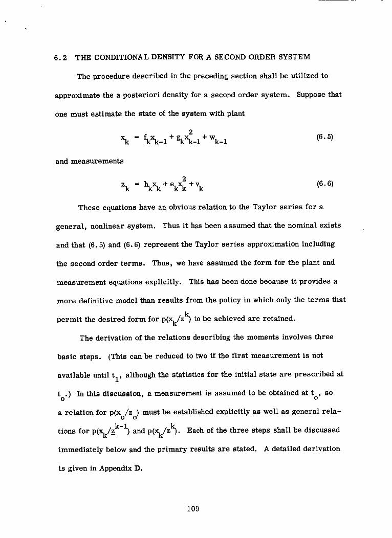
6.2
approximate the a posteriori density for a second order system.
one must estimate the state of the system with plant
2xk = _xk_1+gkxk_l+Wk_1
THE CONDITIONAL DENSITY FOR A SECOND ORDER SYSTEM
The procedure described in the preceding section shall be utilized to
Suppose that
and measurements
(6.5)
2zk = hk_ + ekxk +vk _6.6_
These equations have an obvious relation to the Taylor series for a
general, nonlinear system. Thus it has been assumed that the nominal exists
and that (6.5) and (6.6) represent the Taylor series approximation including
the second order terms. Thus, we have assumed the form for the plant and
measurement equations explicitly. This has been done because it provides a
more definitive model than results from the policy in which only the terms that
permit the desired form for P(Xk/zk) to be achieved are retained.
The derivation of the relations describing the moments involves three
basic steps. (This can be reduced to two if the first measurement is not
available until t 1, although the statistics for the initial state are prescribed at
t .) In this discussion, a measurement is assumed to be obtained at t , soO O
a relation for P(Xo/Zo) must be established explicitly as well as general rela-
k-1 ktions for p(xk/z ) and P(Xk/Z-" ). Each of the three steps shall be discussed
immediately below and the primary results are stated. A detailed derivation
is given in Appendix D.
109

(1) Determination of P(Xo/Zo)
The initial a posteriori density is obtained from (2.15)
P(Zo/Xo) P(X O)
P(Xo/Zo) = p(Zo ) (2.15)
The distribution for the initial state has been assumed to be gaussian. The
conditional density p(Zo/X o) is determined from (6.6) and the distribution for
v k •
p(Zo/Xo) = p(z ° - hoX ° - eoX2o)
2z -h x -e x
1 o oo oo)2k exp- (v 2 rO
Since e is non-zero, this density is obviously no_._tgaussian. This termO
must be approximated in order to obtain a P(Xo/Zo) having the form (6.4).
This approximation is accomplished in the following manner. The p(Zo/Xo)
can be rewritten as
z -hx
1 o 00)2p(Zo/Xo) = k exp-v _( 2r
o
2 3 24
_1 (-2e z x +2h e x +eoXo)o o o o o o } (6.7){exp 2 2
ro
For an alternate approach, refer to Chapter 4. Introduce (6.7) and P(Xo) into
(2.15) and rewrite as
1P(Xo/Zo) = kconeXp-_ (
A
X -
o _o )2 [exp B(xo)]1"[
O
(6.8)
ii0

where kcon
represents terms that are independent of xO
h21 Df o 1
2 2 2r m
O 0 O
h z
I)f 2 oo a= o +r m
O O
(including p(Zo) ), and
2 x 3 4e -2z x +2h +e xDf o oo oo oo
S(Xo) - 2 ( 2 )ro
o
If the measurements were linear, then e would be identically zero ando
and rr2o would be the mean and variance of P(Xo/Zo). Thus, they are a scalax
version of the Kalnmn filter equations.
It is necessary to determine the moments of P(Xo/Zo) from (6.8) in order
to put the a posteriori density into the form required by (6.4). This is not
immediately possible because of the last factor. If exp B(Xo) can be approxi-
mated by a power series, then it becomes a simple matter to determine the
moments. One could approximate this term by
÷ 1 B2(Xo) (6.9)exp B(Xo) = 1 + B(Xo) 2_
Numerical results indicate that this is not an adequate approximation in many
instances. In this chapter, the B is rewritten in terms of the linear estimate
A. That is, one sees from the definition of B that it has the form
0
B(Xo) = b2X2o+b3X3o +b4 4
111
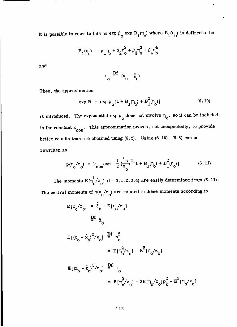
It is possible to rewrite this as exp flo exp Bl(_o) where Bl(rlo) is defined to be
B l(rlo) = fll_o +_ 2rl_ +_ 3_3o + fl4rl4o
and
Df ^= (x° _ )"qo o
Then, the approximation
2exp B = exp flo[1 + Bl(rlo) + Bl(_o)] (6.10)
is introduced. The exponential exp rio does not involve _o' so it can be included
in the constant k . This approximation proves, not unexpectedly, to providecon
better results than are obtained using (6.9). Using (6.10), (6.8) can be
rewritten as
1 rlo2 2
p(_o/Zo) = kconeXp - _ (---=") [1 + BI(_ o) + Bl(_o)]0
(6.11)
The moments E [rllo/Zo ] (i = 0, 1, 2,3,4) are easily determined from (6.11).
The central moments of P(Xo/Zo) are related to these moments according to
= + E ['Qo/Zo]E [xolzol
Df ^= X
0
_o)2/Zo] Df 2E [ (x ° - = Po
= E[rl2o/Zo ] - E2[rlo/Zo]
_o)3/Zo] DfE [ (x ° - = tJ- o
/z - 2 E 3E[Vl3o/Zo ] - 3E[_ ° olPk - [Vlo/Zo]
112

E [(x0 - _o)4/Zo] =Dr _o
= E[_4o/Zo] - 4_toE[_o/Zo] - 6p2oE2[_o/Zo] - E4[_o/Zo]
From (6.4) the approximation to P(Xo/Zo) is seen to be
P(Xo/Zo) = k exp 1 +1o - 2(_o )211 3! c3H3(_o) +_!c4H4(_o)+_'!c3H6(_o)]10 2
where
x-_Df o o
o Po
Df o
e 3 = --_
Po
0-3
c 4 -- _
Po
The complete definition of this density is contained in Table 6.1 and in
Appendix D. To repeat, the principal approximation involved in determining
P(Xo/Zo), aside from the general form, occurs in the simplification of exp B.
This approximation reoccurs in the determination of P(Xk/zk ) from (IV).
k-1(2) Determination of P(Xk/Z )
The prediction density is determined from (2.13).
k-i k-ip%/z ) = p%_l/z )P/Xk/Xkl dXk_1
P k-1Assume that (Xk_l/Z ) has the form prescribed by (6.4).
(6.5) and the density for Wk_ 1 that
(2. 13)
It follows from
113

2
i Xk- _-i - _Xk-1)2 (6.12)P(Xk/Xk_l) = k exp-_(
w qk-1
It becomes clear upon a moments reflection that the integration required by
(2.13) cannot be directly accomplished. Fortunately, this is not necessary.
k-1Because the approximation calls for the moments of P(Xk/Z ), con-
sider their direct calculation from (2.13). For i = 1,2, 3,4,
i- k-i i k-i
_t_/_. I : ..F_p%/_)<_<
Substitute (2.13) into (6.13) and iterate the integrals. Then
i- k-1 zk-1 i / ]EExklzi: .FP%_ll){,Fxkp(xkxk-1)'_'_'k-_
The innermost integration is easily accomplished and produces
2
E[_I:__II: _kxk_1+gkXk_l
: +
3/ 2 2 3EExk__1i: 3O__lCfkxk_l+gkxk_l)+(_xk_I+gk__l)
(6.13)
(6.14)
4 / 4 2 .2 2 2 4EiXkXk_l] = 3qk-1+ 6(_Xk-1+ gk_k-1j %-1 + ¢fk_k-1+ gkxk-1)
The moments E [x_/z k-l] are easily determined from (6.14). To this
point, no approximations have been introduced other than the original assump-
tions associated with the form of P(Xk_l/zk-1) and with (6.5) and (6.6). In
establishing the E [x_/z k-l] , it is found that for this problem, the fifth through
eighth central moments of P(Xk_l/zk-1 ) are required. These have not been
computed (although they could be determined when the first four moments of
114

the a posteriori density are established). To approximate these moments, we
assume that they are identical with the gaussian moments. That is, we let
_5 = ta7 = 0
6
_t6 = 5Pk
This constitutes the only additional assumption involved in determining
/z k-1p(x k ). The equations are summarized in Table 6.1 and Appendix D.
(3) Determination of P(Xk/Z _
The P(Xk/Z _ is determined from (IV).
= (iv)
p(zk/zk'l )
The derivation is quite similar to that provided for P(Xo/Zo) in Section 6.2.1.
In that case, P(Xo) was gaussian, whereas its counterpart in IV (i. e., the
k-1P(Xk/Z ) ) has the Edgeworth form. Thus, the approximation of the factor
exp B(Xk) that arises through the nonlinearities in the measurement device is
performed in exactly the same manner. The algebraic manipulations are
more involved in this case because the Hermite polynomials must be rewritten
in terms of the centered variable
Df ^
^
where {k
is referred to Appendix D.
is the linear estimate. For the details of the derivation, the reader
The general relations that result are stated in
Table 6.1.
115

The moment relations for simpler density approximations are obtained
without difficulty from the tabulated equations. In fact, one obtains another
gaussian, but nonlinear, filter directly by eliminating all of the terms that are
associated with the Hermite polynomials H 3, H4, and H6. This gaussian filter
is distinctly different from that of Chapter 4 and shall be seen to give different
(and more satisfactory) results in Chapter 7.
It is hoped that the discussion has been sufficiently clear to indicate the
ease with which more terms in the Edgeworth series or in the power series
approximation of exp B 1 could be included. This system illustrates all of the
problems that would be encountered in including additional terms in the
expansions.
The relations in Table 6.1 that describe the calculation of the central
moments of a posteriori densities can be described in general by two terms.
The first term represents the moments associated with the linear moments
gk and _ . To these moments are added perturbation terms that account for
the nonlinearities. It may not be immediately obvious that this is the case for
P(Xo/Zo) and P(Xk/zk), but it is more readily seen for P(Xk/zk-1 }. It is
particularly interesting to note the effect of plant nonlinearities on the sym-
k-1metry of the distribution. For the sake of discussion, suppose that P(Xk_i/z )
4is gaussian so that _k-1 is identically zero and '_k-1 is 3Pk_ 1. Then, the
_k/k-i has the form
2^ 4 3 4 4 ^2 6_k/k-1 = 6_gkPk-1 ÷ 33_kgkXk-1Pk-1 + gk (2 Pk-lXk-1- 2Pk-1)
116

Naturally, if the plant is linear, then gk is identically zero and so
k/k-1 = 0.
However, when gk is non-zero, it is clear that _k/k-1 in general will be non-
zero thereby reflecting the loss of symmetry of the distribution. The sym-
metry of P(Xk/Z _ is also destroyed in general by nonlinear measurement
terms. The approximation of the a posteriori density by a gaussian distribu-
tion (e. g., in the case of the Kalman filter) might be suspected of resulting in
a mean value that is biased away from the true mean because of the unsym-
metric nature of the true density. This is seen to indeed to the case in some
of the numerical results of the next chapter.
2, _k' Vk all dependIt should also be noted that the central moments Pk
upon the measurement data because the term Bl(Vlk) contains the data explicitly
in the coefficients. This would have to be taken into account in the derivation
of optimal control policies using this density approximation.
Relations defining the moments of the a posteriort density, particularly
P(Xk/Z_, can be determined using different approximation techniques. Itfor
has already been noted that the exp B(Xk) can be written immediately in a power
series in x k rather than first rewriting it in terms of the centered variable _k:
It is not surprising that the former does not give as good an approximation for
an equivalent number of terms in the power series. Another variation is pos-
sible in the way in which the _k is defined. One can follow the procedure used
in Chapter 4 and include all terms of the second order in x k in the _k and w2k"
Then, one obtains
117
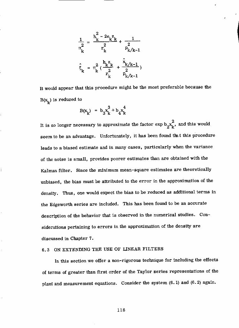
1 h_ - 2ekz k 1_ +
2 2 2
_k rk Pk/k-i
_k = 17k ( _ + 2 )
rk Pk/k-1
It would appear that this procedure might be the most preferable because the
B(Xk) is reduced to
B(Xk) = b3x _ + b4x _
2It is no longer necessary to approximate the factor exp b2Xk, and this would
seem to be an advantage. Unfortunately, it has been found that this procedure
leads to a biased estimate and in many cases, particularly when the variance
of the noise is small, provides poorer estimates than are obtained with the
Kalman filter. Since the minimum mean-square estimates are theoretically
unbiased, the bias must be attributed to the error in the approximation of the
density. Thus, one would expect the bias to be reduced as additional terms in
the Edgeworth series are included. This has been found to be an accurate
description of the behavior that is observed in the numerical studies. Con-
siderations pertaining to errors in the approximation of the density are
discussed in Chapter 7.
6.3 ON EXTENDING THE USE OF LINEAR FILTERS
In this section we offer a non-rigorous technique for including the effects
of terms of greater than first order of the Taylor series representations of the
plant and measurement equations. Consider the system (6.1) and (6.2) again.
118

Assume that a nominal x__ 1
6xk
6z k
where
exists and let (6.1) and (6.2) be represented by
1 x2k + (6.14)= f_6xk_1+_f_'6 -1 Wk-1
1= l_(Sx, k +_hl_'6Xl_ +V k
IX6xk_I = xk_I-x__I
IX
_ xk-fk(__1)
IX
5z k = z k - hk[fk(Xl__l)]
(6.15)
To apply a linear filter, one must represent the evolution of 6 x k by a linear
difference equation and 6 zk by a linear relation with the state. The obvious
procedure for (6.14) and (6.15) is to neglect the second order derivatives f_'
and h_'. Consider an alternative procedure.
At the sampling time tk, one has an estimate of the state 6 Xk_ 1. Let
5 Xk_ 1 be written as
_k-1 = 6_-1 - 6_k-1
Then
6_ = _6__I+_'(__i- 6__i)6__I+Wk_I
} f_, i ~ + wk 1 (6.16)= (fk+ 6xk-1)SXk-1-2 fk'6Xk-laXk-1 -
Now, neglect only the term } f_'5Xk_l. As long as 5 xk_ 1 is sma11
compared with 6Xk-l' one would expect (6.16) to provide a better approxima-
tion of the behavior of the plant than when the second order effects are
119

1neglected entirely. Then, the factor (f_ + _ f_t 6 _k_1 ) will serve as the linear
plant approximation. The prediction of the state at t k is seen to be given by
6Xk/k_1 : + 7 6xk_l)6xk_1 (6.17)
and the variance is
2 1 ^ ,22 2Pk/k-1 = (f_ + 2 _' 5 Xk_l) Pk-1 + qk-1 (6.18)
Compare this result with the more precise relations found in Table 6. l(b).
k-1Suppose that P(Xk_l/Z ) are gaussian so that
_k-1 = 0
4
'Ok_ 1 = 3Pk_ 1
Then, the predicted mean and variance are seen to be
5Xk/k-1 = (fl_ +1 ,, ^ 1.,, 22 fl_ 5 Xk_l) 6 Xk-1 +2 I1¢ Pk-1
and
2 1 _,, ^ 2 2Pk/k-1 = (f_ +2'f'k 5Xk-1) Pk-l+q_-l+_f_ ' 4Pk-1
Thus, the approximations (6.17) and (6.18) are seen to cause the terms
1 fvv 2 and 3 4k _k-1 _ f_v Pk-1 to be neglected from the mean and variance equations,
respectively. In many cases, one would not expect this omission to be
significant.
A similar procedure can be employed for 5 z k. The predicted estimate
Xk/k-1 is used in rewriting (6.15) as
6 Zk = _ + i h_' 5 _/k-1 )6Xk + Vk (6.19)
120

The equations (6.16) and (6.19) are linear in the state perturbations. In
the use of the linear filter, the plant Fk and measurement coefficients Hk can
now be treated as
i -I! ^
Fk __Df_+2_5xk_1
Of course, if the nominal is rectified with 5 Xk-1 at every time tk, then after
the rectification
5Xk_ I = 6 = O.
so the second order derivatives are eliminated.
This technique is applied in Chapter 7 and produces some interesting
results.
121

(a)
TABLE 6.1
The A Posteriori Density Function
The A Posteriori Density P(Xo/Z o) for the Initial Sampling Time
P(Xo/ZO) 1 (Co)2= k exp-_ [io
_O =
10+ _.t c3H3(_o) +_.I c4H4(_o) + _-.I c23H6 (_o) ]
A
X -XO 0
Po
_to
C3 = - -'_
Po
0
c4 =-_-3
Po
Central Moments:
= _ +E['qo/Z o]O 0
Po --
22 E[,qo/Zo] _ E2[_o/Zo ]
3/z - [_o/Zo]p 2 E 3_o = E[Tlo o ] - 3E - [_o/Zo]
4/z .'Co = E[_ ° o ] - 4_oE[_o/Zo] - 6p2oE2[_o/Zo] - E4[_o/Zo]
and
E [_lo/Zo ]
E[n:li i 2
+ E [r_oBl(Tlo)] + E ['NoBl(r_o)]
I+E[BI] +E[B 2]
The expected values are obtained relative to the density
P(rlo) = ,4_'_o
122
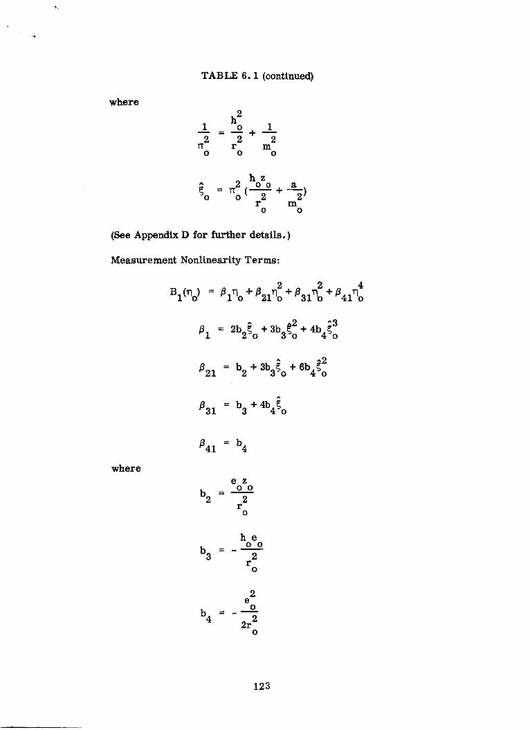
where
TABLE 6.1 (continued)
h21 o 1
2 2 2r m
O o O
h z
2 oo .._--_ (--T+ )_o or m
o o
(See Appendix D for further details. )
Measurement Nonlinearity Terms:
2 2 4
Bl(rlo) = Blrlo + B21rlo + B31r_o +/341rlo
÷
/321 = b2 + 3b3_o + 6b4
A
/331 = b3 + b4_o
where
/341 -- b 4
e zO O
b2 - 2r
o
h eO O
b 3 = _ --_r
o
2e
o
b 4 = __2r 2
o
123
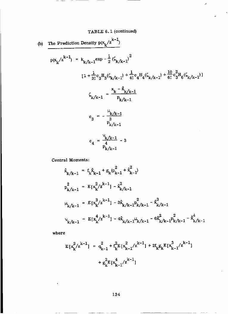
(b)
TABLE 6.1 (continued)
The Prediction Density P(Xk/zk-l)
1 2
P(Xk/Zk-l) = kk/k_lexp - _ (_k/k-i)
1 I0 2 -[i + _. c3H3(_k/k_ I)+ _, c4H4(%/k_ I) + _.,-.,c3H6 (_k/k-1)]
_k/k-1 -Pk/k-1
_k/k-ic3 3
Pk/k-1
=_-3c4 4
Pk/k-1
Central Moments:
: + +
2 = E 2. k-1 ,,2Pk/k-1 [Xk/Z ] - Xk/k-1
= E 3/zk-1 " 2 ,,3_k/k-i [Xk ] - 3xk/k-lpk/k-I - Xk/k-i
Vk/k-i
where
2- k-1E [xk/z 1
4-k-i ^
= ZlXk/Z ] - 4Xk/k_lUk/k_ 1
2 _ 2 - k-i= qk-1 + E[Xk_l/Z ]
6^2 2- Xk/k-lPk/k-1- 4/k-1
+ 2f.kgkE[__l/zk-l]
2 4 , k-1
+ gk E [Xk_i/z l
124

and
TABLE 6.1 (continued)
3-k-1 2 ^ .3El 3 /zk-1] + 3_gkE [ 4 /zk-1]: _%__Xk/k__z[_/_ I +% Xk-1 Xk-I
3_k_Z,5 /,k_,,+,_Z,4/,k-,,+ Xk_1 -
.4E( 4 /zk-1)+,,E,__/-1_1_'_+_ _-_
+ _%_.(__i/_)+ _-i
+_¢.4_,,,,.,.-_,,-¢_4_,,,,.'-_,
(_ 2 +^2z _/k-l) = Pk-1 Xk-1
^3 2E(x__i/k =1) " ,_ + 10Xk_lPk_ I= _k-1k-1+io i_k_i
'_,4-/-" ° '_&"k-'÷_°'_= 5pk_1+ Xk_l__l
_1 p ^6+15 - k-1 +xk-1
Eta,1/k-ll = ^ 6 + +
2.^ 5 2 ^7+ LXk_IPk-i + :_-i
t s /k-11 =E Xk_ 1
,,5
+xk_ 1
7Pk_ I + _ -
28 _6 2 ^8+ __1%_i + _-i
125

(c)
TABLE 6.1 (continued)
The A Posteriori Density P(Xk/Z_
1- +_'. c3H6(_k) lP(Xk/zk ) = kk exp _ (%)2[ 1 + _,.c3H3(_ k) + _.,c4H4(%) i0 2
_k =Pk
c3 =--" {Pk
--_-sc4 4
Pk
Central Moments:
2 2/zk.Pk = E[_ j
3/zk
- E [_k/Z k]
3E [_]k/zk] pk E 3 /z k-_ _ [_ J
_k = E[_/_k] - %E[_/_'k]- 6p_S2[_/zk]- _4[_/_k]
where
B(_)= 2Df 1 + BI(_ k) + B l(_k)
= 3_ c 1 i0 2Df i + 3Hs(BR) + _.,c4H4(_ k) + _. CsH6(B k)
126

TABLE 6.i (continued)
2 2 2
_k rk Pk/k-1
^ 2 _"k + _/k-1_k = nk ( 2 2 )
rk Pk/k-1
The BI(Tlo) are defined in the same manner as in Part I with the
trivial change of subscript. The Hi(_k) and the E [v_/z k] are defined
in Appendix D.
127

, ppRECED_G pAGE BLANK NOT FkME •
CHAPTER SEVEN
NUMERICAL COMPARISON OF LINEAR AND NONLINEAR
FILTERING TECHNIQUES
It has already been pointed out that simpler approximations can be
obtained from the density approximation described in the preceding chapter by
neglecting either terms of the Edgeworth expansion or terms of the power
series expansion of exp B(Xk). Each of the approximations in the resulting
hierarchy describe a minimum mean-square estimator (i. e., the conditional
mean provides the estimate). In this chapter, the adequacy of each density
approximation is investigated by examining the behavior of the estimates of
the state of a dynamical system. These estimates are compared with those
obtained from the linear estimator of Chapter 3, the nonlinear estimator of
Chapter 4, and the modified linear estimator of Section 6.3. The system that
is considered is simple. Nonetheless, it appears to illustrate the important
characteristics as clearly as the more complicated systems that have been
investigated.
The mathematical model and the computer program are described briefly
in Section 7.1. The parameters and estimation policies that are considered
are also discussed. The approximation of the true P(Xk/Z _ by a gaussian
density provides an interesting class of filters. They are discussed in
Section 7.2. The filters resulting from the Edgeworth expansion approxima-
tion (i. e., the nongaussian version) are investigated in Section 7.3. Conclu-
sions suggested by the results of Sections 7.2 and 7.3 are stated and
discussed in Section 7.4.
129

7.1 THE GENERAL PROBLEM
Consider a scalar system with plant described by
= xk_I+wk_1 (7.i)
The state is to be estimated from measurement data that are related to the
state according to
2zk = x k+v k (k=0,1,...) (7.2)
The initial state x and the plant and measurement noise sequences w., v.o J 3
are gaussian with known statistics.
E[Xol = a
_ 2E[(x ° a) 2] = mo
E[Vk] = 0 = E[Wk] for allk
2 2 2EIv ] = r k ; E[Wk] = qk
2 2 2The variances m o, r k, qk will constitute the basic parameters for the
2 2 2
study. The mo and r k will always be greater than zero, whereas qk will be
set equal to zero in many cases. The actual values assigned to these param-
eters will be specified later.
The estimation policies are based upon the use of perturbation theory.
Two different nominals will be utilized. First, the nominal will be chosen to
be E [Xo], and this value will be retained throughout the observation policy.
As an alternative choice, the nominal will be rectified at each sampling time to
be the minimum mean-square estimate (as in Chapter 5). The results obtained
with each of these choices for the nominal will be compared. In each case,
130

the perturbation equations have the form
6_k = 6,,__i+_k_I
26,.k = + +
where
_"_-1= "_-1-"_-1
6xk =Xk-q
(7.3)
(7.4)
A digital computer program was developed to simulate this system and
to exercise several different estimation policies. The initial state and the
noise sequences were obtained from a gaussian random number generator [61].
All of the computations were accomplished using double precision arithmetic.
The results that appear in subsequent sections represent a single
realization of the random sequence. The size of the computer program
coupled with the nature of the double precision computations on the particular
IBM 7040 that was used precluded the possibility of a complete Monte Carlo
simulation. That is, it did not appear to be feasible to obtain the number of
runs necessary to compute significant sample means and variances (i. e.,
apparently at least 1000 realizations are required [31]). Instead, the data
presented below represent the behavior of each filter when the same noise
sequences are encountered. It is reasonable to expect in the comparison of two
filters that the one that gives the better response for a given noise realization
will be generally more effective. Enough cases were simulated to indicate
131
that the results that are presented are representative of the type of behavior
that shouldbe expected.
The filter configurations that are examined are to a major extent obtained
from the density approximation derived in Chapter 6. As has been mentioned
earlier, different density approximations are obtained from the most general
expression by eliminating the Hermite polynomial terms (i. e., H6, H4, H3)
and/or by including only one term in the power series expansion of exp B
rather than two. Additional density approximations are provided by the results
of Chapter 4. This gaussian approximation is investigated in Section 7.2 to
show the effect of different approaches and to indicate that not all approxima-
tions should be expected to provide satisfactory results.
7.2 FILTERS BASED UPON A GAUSSIAN DENSITY
Four different filters are investigated in this section; two of them are
linear whereas the _ther two are not.
(G-l) Linear (Kalman filter): This filter is described in Chapter 3.
(G-2) Linear filter with modified system matrices: The Kalman filter
is utilized, but the system matrices are modified in accordance
with the discussion of Section 6.3. In this example, the linear
relation between the measurement and state perturbations is
=
132

(G-3) Gaussian nonlinear filter Number 1: The Hermtte polynomial
terms H3, H4, and H6 are eliminated and the linear moments
are modified because of the presence of the nonlinear measure-
ment term exp B. See Section 6.2 for further discussion.
(G-4) Gaussian nonlinear filter Number 2: The gaussian approximation
of Chapter 4 is considered.
These four filter configurations were exercised with a variety of noise
realizations and a priori statistics. The results for a particular noise
realization is depicted in Figures 7.1 through 7.3. These data indicate the
relative behavior of the filters when acting upon the same measurement data.
The system yielding the results shown in Figure 7.1 contained no plant
noise. The standard deviation of the initial perturbation was assumed to be
10 percent of the mean value of the initial state.
E[Xo] = 1
E[(x °- 1)2] Dr= m2O
= 0.01
The initial perturbation was obtained from a gaussian random number generator
and was
5x = -0.044789270
Before an observation is processed, the estimate of the perturbation is zero,
so the initial error is 6 x .O
In Figure 7. l(a), the measurement noise has a standard deviation equal
to 1 percent of the nominal state
133

EE J= 0. 0001
The standard deviation of the error in the estimate (i. e., pk ) was found
to be approximately the same for all configurations. Thus, only the standard
deviation from the linear filter (i. e., Case G-l) was plotted.
Note first that the error in the linear estimate exceeds the statistic on
the eleventh measurement and remains larger thereafter. Although taken by
itself, this behavior is not impossible, it nonetheless describes a common
occurrence in the application of linear filters to nonlinear problems. As was
noted in Chapter 5, a sufficiently accurate measurement device will often
cause the statistic to be a poor measure of the actual error because of the
importance of the neglected nonlinear effects [ 31 ].
The general character of the response of filters (G-2) and (G-3) is simi-
lar to that observed with (G-l), but the magnitude of the error is considerably
reduced for these two configurations. It is of further interest to note that
(G-2) and (G-3) give essentially the same results.
When the filter of Chapter 4 is used, the results are very disappointing.
In fact, the error inthe estimate is seen to be considerably increased and
suggests that the estimate contains a bias error. Since the conditional mean
is theoretically unbiased, a bias error could enter only because the approxi-
mation of the true density is poor. One would expect that the error would be
decreased by improving the density approximation. Although not discussed at
length here, such an improvement was attempted and the response was observed
to improve.
134

m
m
I
0
I
I!1
0
0
I I o
0
Ic_I
135

The results shown in Figure 7. l(a) are based upon a single prespectfied
nominal. The filter response, when the nominal is rectified at each sampling
time, can be seen by referring to Figure 7. l(b).
Cases (G-l) and (G-2) are theoretically identical.
Under this condition,
It is particularly interesting
to observe that Case (G-l) in Figure 7. l(b) is essentially identical with Case
(G-2) of Figure 7. l(a). Thus, the modification of the system matrices for
policies based on a single nominal has the same effect as rectification of the
nominal at each sampling time.
Rectification of the nominal is seen to cause all four cases to give
basically the same results. This implies that the nonlinear effects are
eliminated to a major extent. This becomes more true as the number of
samples that have been processed increases.
The standard deviation of measurement noise is increased from 0.01 to
0.1 for the results shown in Figure 7.1(c). One observes that the four filter
configurations provide very similar behavior. This result indicates that the
magnitude of the measurement noise is more significant than the nonlinearities.
Further verification of this statement was provided by finding that rectifica-
tion does not appreciably influence the results. These data have not been
included.
When noise is included in the plant, the filter response is affected in a
striking manner. As is known, the presence of plant noise prevents the error
variance from vanishing and causes it to approach some nonzero value. As is
seen in Figure 7.2, plant noise with a variance of 0. 0001 leads to a limiting
136

cq
t>--'"
o L L,c; c; _ c/
z01 x eqmnT:_B.wuT .m.la[/[
o
{CDnn
o_
,.-4
Lu
137

c'qoo I
rn v
""4 I I I
I I I I
°-__or,,l
e&
!l°illo. ,
I I
)
m
C
P m
!_
m
I s
, /
, I
_I0 v _ C'g
iOi x e_nI_e_t ul -TO-_-_Ot
8
O)
r_
° I
!
138

value of approximately
within three samples.
Pco _ 0.00455
One is hard-pressed to judge that one filter provides a
more satisfactory response than any other. Naturally, as the level of plant
noise decreases, one approaches the behavior shown in Figure 7. l(a). It was
also found that rectification does not affect the results of Figure 7.2 in any
significant manner.
2The nonlinear effects can be amplified by increasing m since the initial
o
state perturbation is based upon the initial statistics. To obtain an additional
2insight into these effects, the m was chosen to be
O
2m =0.1
O
This led to an initial perturbation of
8x = -0.14163609o
The behavior observed in Figure 7. l(a) is aggravated by this increased pertur-
bation. The results for a noise-free plant, measurement noise variance of
0.0001, and prespecified nominal are depicted in Figure 7.3. The inadequacy
of the standard deviation Pk as a measure of the error is revealed more clearly
than in the preceding data. The linear filter (G-I) and the filter (G-4) are seen
to exhibit a definite bias because of the lnvariance of the error. The fact that
(G-4) leads to a deterioration of the accuracy of the estimate is even more
apparent. Possibly the most interesting aspect of these data stems from the
realization that the modified linear filter (G-2) produces consistently better
139

140

IZII
I
f
I
f
!
l
I
i-I I
°
I
•_J ,,i
°_ _
I
I
I
X%
/
JJ
UI I
_ d
m
A _ _ A
l I I I
I I I I I
i
gOI x o_nT_SH UT -_o_._
oo
0
I
0
_8
m
0
0
141

results than the nonlinear filter (G-3). However, all of the filters lead to
results that consistently disagree with Pk" This case will be discussed further
in the next section.
One would expect, judging from past results, that rectification would
improve the filter performance. It is noteworthy that when the nominal is
rectified, the results do improve and, in fact, the response is described quite
adequately by (G-2) in Figure 7.3. Thus, once again for this example, Case
(G-2) appears to be equivalent with rectification of the nominal.
7.3 ESTIMATORS BASED UPON NONGAUSSIAN DENSITIES
In this section, the Kalman filter is compared v_ th the filters provided
by the Edgeworth series approximations. The results are based upon the
approximation
1 2expB 1 _ I+B I+_.,B 1
where B 1 is defined in Chapter 6. It was found that it was necessary in most
instances to use the two-term approximation as opposed to
expB 1 _ I+B 1
in order to obtain sensible behavior for the second and fourth central moments.
This aspect is discussed briefly in Section 7.3.2.
The nonlinear filters are identified by the highest order Hermtte poly-
nomial that is included. Thus, the estimate provided by most general expan-
sion is referred to as the H 6 filter. Simpler models for the nongaussian
densities yield, then, the H 3 and H4 filters.
142

7.3. i Nonlinear a Nongaussian Filters
Let us consider the response of this group of nonlinear filters for the
cases investigated in the preceding section. In all of these cases, let
E [Xo] = i
First, suppose that
2m = 0.01
O
2
rk = 0.0001
2
qk=O
The initial perturbation is
5x = -0.04478927o
and the measurement noise realization is identical with that contained in the
data of Figure 7.1.
The results based on the Kalman filter that were included in Figure 7.1
are repeated in Figure 7.4. It was found that the gaussian, nonlinear filter
and the H3 filter provided essentially the same response. This is seen by
comparing Figure 7.1 and 7.4. In addition, the H4 filter exhibited essentially
the same response as the H6 filter. Possibly the most significant difference
that is observed is that Pk for the H4 and H6 filters is considerably larger than
for any of the lower order filters. This results in a greater sensitivity of the
conditional mean to current measurements. This is reflected, unfortunately,
by the larger error that is observed during the fourteenth through seventeenth
samples. The error is compatible with the statistic Pk' however.
143
A prespecified nominal is used in the data for Figure 7.4(a). When the
nominal is rectified, the results obtained with all of the filters tend to be
essentially the same. These data are depicted in Figure 7.4(b) and again
indicate the manner in which rectification seems to eliminate the nonlinear
effects.
When the measurement noise is increased (as was done in Figure 7.1(c) ),
the linear filter gives the same response as the gaussian, nonlinear filter
(G-3) and as the H3 filter. The H4 and H6 filter again are adversely affected
during the fourteenth through seventeenth samples.
Plant noise causes the same response for the H3, H4, and H6 filters as
was described for the nonlinear gaussian filter (G-3) in the preceding section.
These results will not be repeated here.
When the nonlinearity is made more significant by increasing the state
perturbation, the nonlinear filters are seen to provide a response that is con-
siderably different from that observed for the gausstan estimators. As seen
in Figure 7.5(a), the Pk for the H3, H4, and H6 filters is larger than for the
gausstan filters. Thus, the Pk appears to be a more accurate measure of the
error for these filters. Also note that the Pk is a random variable for the
nonlinear filters, so the Pk is not as well-behaved. Comparison of Figures
7.3 and 7.5 indicate that the error in the estimate from the modified linear
filter (G-2) is subject to less violent changes, but that the H. filters givel
estimates that appear to cope with the nonlinearity more adequately. These
filters are more sensitive to the actual measurement noise, however.
144

QO
M
!I
III/IIII
IIIIIIII
I
I
0
m
0
0
o
0
v
Ol,li
I ! I I
I
145
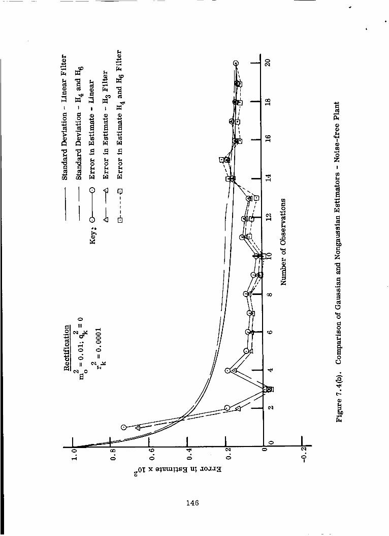
I
co.,,=4
0
!
0
*_...I
Ill
txO
0
r_
II1
0r_
.2.
.,..4
I i
_OI x _a!_s_ u_ ._o.x_
I
I
146

I I I I I
0 0
m IlQ _
,_ °°_
01
!!°III-- 0
I I0 (2o
•.; c;
oo
¢)oo
,,g
Icg
e
I
(1)O)
I(1)
0
I
0
m
r_
0
0
0r_
A
ov
,ql
147

Orbit rectification improves the estimate for every case but particularly
for the linear filter. The H4 and H 6 filters appear to provide the better res-
ponse during a major portion of the interval. However, these filters again
are more sensitive to the large measurement noise values that are present in
the fourteenth through seventeenth samples. These results are presented in
Figure 7.5(b).
7.3.2 A Poor Density Approximation
One difficulty manifested itself in some of the cases that were simulated
although not in any of the results that have been presented above. It was found
that the second and fourth central moments occasionally assumed negative
values. This was observed for every one of the nongausstan filters, although
it occurred most frequently among the approximations that used
exp B I = i + B I.
The inclusion of the second order term eliminated the problem to a major
extent, although it did not eliminate it entirely when a large state perturbation
was experienced. This suggests that it might be appropriate to include the
third order term (i. e., 1/3! B31) in order to improve the approximation of
exp B 1. Alternatively, the negative moments could be interpreted as implying
that additional terms of the Edgeworth expansion should be included in order to
of P(Xk/Z _. As has been pointed out, the truncatedimprove the approximation
Edgeworth expansion is not a true density because negative values are assumed
for some values of x k. This could result in erroneous values for the moments.
148

I I I I I
0 0
I °
I I I I I I I I o
_OT _ _,_p,e_ _z_.zo.z.z:_
149

q
I I I I I I
iii .oo
0
0
e_ oi_ i . 0
ml c_laEtoc_._
@
n I I Ir.D _ ¢q 0
I/
/
/I
/
I I I I• • ° °
0 0 0 0
_OI x o:_m_aT_e H u I .XO.LZH
150

7.4 SUMMARY OF RESULTS
Several conclusions can be drawn from the numerical results of the
preceding sections. Although the data are based on a very simple system,
more complicated systems have been investigated and appear to corroborate
the conclusions that are stated below.
Before proceeding to any statements regarding the merits and demerits of
the various estimation policies, it is necessary to recognize the following.
(0) Unless the measurement noise and/or the plant noise is "small",
the linear filter gives essentially the same result as the considerably
more complicated nonlinear filters. No attempt shall be made to
clarify the circumstances which one can determine if the noise is
sufficiently "small" to warrant consideration of the nonlinear
filter.
With this provision in mind, it is possible to consider the relative behavior of
the filter configurations.
Of the three conclusions stated at the end of Chapter 5, the one dealing
with rectification is further substantiated in this chapter, and the one dealing
with the nonlinear filter of Chapter 4 can be strengthened.
(1) Rectification of the nominal at each sampling time causes the
behavior of the linear filter to be considerably improved. After
a sufficiently large number of measurement samples, the linear
filter yields essentially the same response as considerably more
complicated systems.
151

(2) The gaussian, nonlinear filter of Chapter 4 is not satisfactory.
It does, in fact, appear to yield an estimate that contains a bias
which causes it to yield poorer results than even the linear filter.
Thus, one must be cautious when deriving an approximation of
a posteriori density.
Several other significant results were obtained. The filter configuration (G-2)
based upon modification of the linear system matrices and concomitant applica-
tion of the linear filter provided a number of suggestive results.
(3) The filter configuration (G-2) yields the same behavior for the
prespecified nominal that is observed when rectification of the
nominal is introduced. This estimation policy was utilized in
Chapter 5, but did not provide such striking results. This can be
attributed to the fact that the plant nonlinearities were not included
in the modification of the system matrices because of the inherent
difficulties. As was observed, it was these effects that were
dominant, however.
(4) The gaussian nonlinear filter obtained from the general approxima-
tion of Chapter 6 yielded results that are comparable with (G-3).
Since the filter (G-3) involves many more computations, one would
question its usefulness. It might prove useful in the determination
of a control policy if one were dealing with that problem.
The Edgeworth approximation provided three filter configurations.
Their behavior shall be summarized in the following manner.
152

(5) The tt4 and H6 filters yielded esse_tally identical results, whereas
H3 can be more closely identified with the gaussian nonlinear
filter (G-3).
(6) The conditional variance is generally larger than that for the
linear and other lower order filters, and in many cases appears
to be a more adequate measure of the error in the estimate.
(7) The estimation error for the H6 filter is more sensitive to the
measurement noise realization than is the lower order filters.
This would appear to be a manifestation of the larger values
observed for the variance.
The sensitivity of the filter response to the method of approximation is
certainly an important consideration. For the example discussed in this
chapter, the following conclusions become apparent.
(8) The approximation of the nonlinear measurement effects (i. e., the
factor exp B1) is of supreme importance. It was found that the
B 1 should be written in terms of the centered variable
k-:k
where Ck is the linear estimate rather than leaving it as a poly-
nomial in x k. Furthermore, the number of terms retained in the
power series approximation of exp B 1 also has a significant effect.
In general, at least terms including the quadratic must be included.
153

It was found that the quality of the approximation of exp B 1 could be
judged to an extent by the behavior of the second and fourth central moments
_k and Vk" These quantities, which should be positive, sometimes assumed
negative values. This was particularly true when exp B 1 was approximated
by the first order terms of the power series.
154

CHAPTER EIGHT
SUMMARY AND CONCLUDING REMARKS
The general problem of determining the optimal control policy for a
stochastic, time-discrete, dynamical system was posed in Chapter 1. The
general solution of this problem, assuming knowledge of the a posteriori den-
sity P(Xk/Z_, was presented in Chapter 2, but more specialized problems
were considered thereafter. Attention was restricted primarily to the prob-
approximating the density p(_k/_Z_. The adequacy of each approximationlem of
was evaluated by examining the behavior of the resulting minimum mean-
square estimate. Estimates from both linear and nonlinear filters were
compared. The class of linear filters that were considered included several
that are based on techniques for extending the range of applicability of the
general linear theory.
In the following section, the problem dealt with in each of the preceding
chapters is described, and the principal results are summarized. The major
conclusions of the study and suggestions for future research are discussed in
Section 8.2.
8.1 SUMMARY
CHAPTER 1: The optimal stochastic control problem is described in the
following manner.
according to
where _k-1
Suppose that the state of a dynamical system evolves
is the control vector and .W.k_l is a random sequence with known
155

statistics.
by
The control policy is to be based upon measurement data described
"_k = -hk(-'_' Y-k) (II)
where Xk is another random sequence, independent of the -_'k-l' with known
statistics. Then, choose the control vectors to minimize the expected value of
N
vN = wi%, i-ll (InE i=1
The general approach to the solution of this problem and the related problem
of state estimation is then described.
CHAPTER 2: The general stochastic control problem stated in Chapter 1 is
considered. In particular, it is shown that knowledge of the a posteriori den-
sity p_k/z_ provides the general solution of the minimum mean-square error
and the stochastic control problem. The p(_x_/z_ isestimation problem then
shown to evolve according to an integral recurrence relation. Relations des-
cribing the prediction and smoothing densities p(___+y/Z_ and p(..Xk_y/Z _ are
also derived. In some instances, the application of the general relations to
a specific system is simplified by working with the equivalent relations involv-
ing characteristic functions. These relations are derived.
CHAPTER 3: The linear, gaussian, optimal stochastic control problem is
considered. It is shown that the solution of this problem separates into the
dissimilar problems of state estimation and deterministic, optimal control.
Furthermore, it is seen that the separation occurs because the error covari-
ance matrix of the estimation problem does no__._tinvolve the measurement data.
156
The solutions of the three aspects of the linear estimation problems (i. e.,
smoothing, filtering, and prediction) are presented.
CHAPTER 4: Attention is restricted primarily to the problem of approximating
the a posteriort density for a system with the plant equation
and the measurement data
-- + (I-N)
=
The noise sequences are assumed to be gaussian and the approximation
is established under the constraint that the density pQxk/z _ is gaussian. This
procedure leads to a generalization of the Kalman filter of Chapter 3. It is seen
that the error covariance matrix becomes a function of the measurement data.
Furthermore, it is seen that the choice of the most recent minimum mean-
square estimate as the nominal leads to a considerable simplification of the
equations.
The problem of determining the control policy for a linear plant from
measurements that bear a nonlinear relation to the state is considered briefly.
It is suggested that the Separation Principle for completely linear systems is
no longer valid because of the dependence of the error covariance matrix upon
the measurement data.
CHAPTER 5: The problem of estimating the state of a spacecraft in a nearly
circular orbit from the angular measurements provided by a horizon sensor
is considered. A nominal is assumed and the results of Chapters 3 and 4 are
157

utilized in this numerical investigation. Several estimation policies are
implemented. Briefly, these policies are-
(l) Kalman filter using a single prespecified nominal
A
(2) Kalman filter using the _Xk_1 as the nominal at each sampling time
tk (the policy of updating the nominal is referred to as rectifica-
tion)
(3) Kalman filter with modified system matrices and prespectfied
nominal (the manner in which the system matrices are modified
is discussed in more detail in Section 6.3)
(4) Continual re-estimation of the initial state using linear theory
with subsequent updating of the estimate of _k using the nonlinear
plant equations
(5)
(6)
Rectification using a smoothed estimate
Nonlinear filter of Chapter 4 (referred to as (G-4) with a pre-
specified nominal)
Nonlinear filter (G-4) with rectification.(7)
Of these seven estimation policies, rectification was found to significantly
extend the range of linear theory and provided the most satisfactory results in
those cases in which policy (1) was found to be inadequate. Policy (4) was also
seen to provide excellent results and has the advantage over the rectification
policy that the system matrices do not have to be recomputed at each sampling
time. It was established that the estimates provided by the nonlinear filter did
not, in general, differ from those obtained with the linear filter. Only the
158

nonlinear measurementeffects were included, however, so this apparent
ineffectualness could be attributed in part to the dominant role played by the
plant nonlinearities. This filter is discussed further in Chapter 7.
CHAPTER 6: A procedure for approximating the a posteriori density P(Xk/Z _
is proposed. It is suggested that this procedure be implemented using a
truncation of an Edgeworth series to approximate the density at each sampling
time. The P(Xk/Z _ associated with a second order, scalar system
2
xk = fkXk_l + gkXk_l + Wk_ 1
zk = hkX k+ek_+v k
where Wk_ I and vk are gausslan is approximated by establishing recurrence
relations for the firstfour moments of the distribution. Itis shown that the
moments for the prediction density P(Xk/zk- _ can be obtained without difficulty.
It is necessary to approximate the nonlinear measurement effects which appear
as a factor exp B. This is accomplished by expressing B as a polynomial in
terms of the variable
where _k is the linear estimate of xk, and then expressing exp B I as a power
series
i 2expB I = I+BI+2-_BI+...
Several different approximations can be obtained from the general result of
this chapter including a gaussian approximation that differs from that found in
Chapter 4.
159

Finally, a technique is suggestedfor improving the approximation
provided by linear theory. This procedure results in the use of second order
terms of the Taylor series expansion of the plant and measurement equations.
CHAPTER 7: The filters deriving from the density approximations of Chapters
3, 4, and 6 are applied to the problem of estimating the state of the system.
= k-1+Wk-1
2
-- k+vk
R was found that the variance of the plant and/or the measurement noise had
to be "sufficientlyN small before the nonlinear filtersprovided results that
differed significantlyfrom those obtained with the linear filter. In the eases
in which the linear and nonlinear filtersgave different results, the response of
the linear filterwas benefitted significantlyby rectificationof the nominal.
Furthermore, the filterof Chapter 4 was observed to yield generally unsatis-
factory results. The estimate provided by this approximation appeared to be
biased.
The gausslan filterobtained from the general results in Chapter 6 gave
satisfactory results in most cases but did not perform significantlybetter
than the modified linear filter. In fact, the modified linear filterappeared to
provide the same behavior with a single prespecified nominal that the linear
filterexhibited with rectification. The two policies result in essentially
equivalent response.
q
160

The most general nonlinear filter consistently yielded values for the
conditional variance that were larger than those obtained from the linear filter.
In many cases, the larger values appeared to more adequately describe the
error. This filter was more sensitive to the magnitude of the actual measure-
ment noise realization. A more complete summary and discussion of the
numerical results is given in Section 7.4.
8.2 GENERAL CONCLUSIONS AND SUGGESTIONS FOR FUTURE RESEARCH
A procedure for approximating the a posteriori density function has been
suggested and has been seen to lead to a straightforward means of accomplish-
ing this objective. Several questions arise concerning the quality of the
approximations that result. The behavior of the specific approximations con-
sidered in this investigation and the conclusions that derive therefrom are
discussed in Section 7.4 and shall no_ttbe restated here. In the remaining
paragraphs, some general questions relating to the application of the theory
and the method of approach are discussed. Topics that require additional
investigation and areas for future research are included throughout the
discussion.
I. The mathematical model upon which the study is based assumes a time-
discrete formulation. Some of the reasons for the use of this model have been
discussed in Chapter 1. On the other hand, one major difficulty is created by
the use of a time-discrete model that must be overcome before the theory can
be applied. In particular, many dynamical systems are described by differen-
tial equations rather than difference equations. Although these differential
161

equations can be solved numerically, it is often impossible to obtain an analytic
form for the solution. Thus, the application of the perturbation theory sug-
gested here is complicated by the difficulties inherent in determining the partial
derivatives required for the Taylor series expansion of the plant equation.
This difficulty is circumvented in using a linear theory by performing the
linearization in terms of the differential equations. It is, then, a straight-
forward matter to establish the state transition matrix and thereby to establish
a linear difference equation. It was seen in Chapter 5 that the nonlinear plant
effects can be dominant if specialized techniques such as rectification cannot
be used. Thus, this aspect cannot be ignored and would appear to require
considerable additional research.
IIo The relations that are obtained by the application d this nonlinear pertur-
bation theory are considerably more involved than the well-known results for
linear systems. Their implementation for use with a multidimensional sys-
tem would appear to lead to a significant computational burden. Thus, one
should examine the possibility of developing special techniques that would
enable the utilization of linear theory for problems which at first glance would
seem to require more sophisticated methods. This has been shown by example
to be possible for estimation problems. It is not clear if analogous policies
can be developed for systems involving control considerations that will
prove to be as fruitful. In many control problems, the nominal control policy
is selected so that prescribed trajectory constraints are satisfied. Thus, one
cannot arbitrarily modify the nominal without first verifying that the constraints
162

will be satisfied by the new nominal. This restriction would seriously hamper
the use of a rectification policy. Thus, the development of specialized methods
for extending the range of applicability of linear theory for control problems
appears to be worthy of consideration.
III. The validity of the approximations has been tested by observing the
behavior of the conditional mean (i. e., the minimum mean-square estimate)
for specific nonlinear systems. It has been found that the estimates behave
satisfactorily in many cases and do provide an improvement relative to the
output of a linear filter. However, the approximations were observed to
deteriorate quite radically for many problems in which the nonlinear plant and
measurement effects were large. The deterioration was marked by the appear-
ance of negative values for the second and fourth central moments. Since
this is theoretically impossible, such behavior must be attributed to the in-
accuracy of the approximation. The truncated Edgeworth series that were
used for the approximation are not true probability density functions because
they can assume negative values for some values of the argument. These
approximations do not provide the only possibility that could be investigated.
interesting to assume that P(Xk/Z _ belongs to a particular class ofIt would be
parametric distributions (e. g., the Pearson distributions). The parameters
would then be determined from the system characteristics. The use of a true
density for the approximation might cause the moments to behave more
satisfactorily.
163
IV. Examination of the behavior of the moments provides an indirect method
of judging the quality of the approximation. It would be desirable to compare
the approximation with the actual a posteriori density. This could be done for
a simple system with a static plant and nonlinear measurements corrupted by
gaussian noise. That is, consider the system
x k = x for all k
zk = hk(X) + v k
Let x and v k be gaussian and independent.
be written as
p(zk/x) p(x)p(x/z_ =
p(z_
It is possible to form p(zk/x) and p(x) and
p( .b : rp(zk/x)p(x)
so the density can be written explicitly.
The a posteriori density can
k 1 z i - h(x) 2
= II exp-_ [ ri " ]P(zk/x) kk i = i
and
p(x) = k exp- 1 x-a 2xO
Thus, one could compute p(zk/x) for this simple system and compare it with
the results given by the approximation. One could also examine the p(zk/x)
to determine some asymptotic properties of the density and verify that the
approximation exhibits these characteristics.
164

V. Little consideration has been givento the problem of establishing control
policies for nonlinear systems. In Chapter 4, it was suggested that the
Separation Principle is not valid for a linear plant when the measurements are
nonlinear. The density approximation of Chapter 6 could be used to develop
perturbative control laws, and it would be interesting to investigate the policies
that result. In fact, these approximations might have their greatest use in the
development of nonlinear stochastic control policies. This should provide a
fertile area for future investigations.
165

.
.
1
.
.
.
.
e
B
10.
11.
12.
REFERENCES
Bellman, R. and R. Kalaba, "A Mathematical Theory of Adaptive
Control Processes," Proc. Nat. Acad. Set., Vol. 45, 1959,
pp. 1288-1290.
Bellman, R., Adaptive Control Processes: A Guided Tour, Princeton
University Press, Princeton, New Jersey, 1961.
Zadeh, L. A. and C. A. Desoer, Linear System Theory: The State
Space Approach, McGraw-Hill, New York, 1963.
Fel'dbaum, A. A., "Dual Control Theory - I," Automation and Remote
Control, Vol. 21, No. 9, September 1960, pp. 874-880, (translation).
Fel'dbaum, A. A., "Dual Control Theory - II," Automation and
Remote Control, Vol. 21, No. 11, November 1960, pp. 1033-1039,
(translation).
Fel'dbaum, A. A., "Dual Control Theory - HI," Automation and
Remote Control, Vol. 22, No. 1, January 1961, pp. 1-12,
(translation).
Fel'dbaum, A. A., "Dual Control Theory - IV," Automation and
Remote Control, Vol. 22, No. 2, February 1961, pp. 109-121,
(translation).
Fel'dbaum, A. A., "On the Optimal Control of Markov Objects,"
Automation and Remote Control, Vol. 23, No. 8, August 1962,
pp. 927-941, (translation).
Fel'dbaum, A. A., Optimal Control Systems, (Translated by
A. Kraiman), Academic Press, New York, 1965.
J
Cramer, H., Mathematical Methods of Statistics, Princeton University
Press, Princeton, New Jersey, 1961.
Sherman, S., "Non-Mean-Square Error Criteria," IRE Trans. on
Information Theory, IT-4, 125-126, 1958.
Cox, H., "On the Estimation of State Variables and Parameters for
Noisy Dynamic Systems," IEEE Trans. on Auto. Control, AC-9, No. 1,
January 1964, pp. 5-12.
167

13.
14.
15.
16.
17.
18.
19.
20.
21.
22.
23.
24.
25.
Sworder, D. D.,
Control Systems,
UCLA, 1964.
Synthesis of Optimal_ Discrete Time D AdaptivePh.D. Dissertation, Dept. of Engineering,
Sworder, D. D., Optimal Adaptive Control Systems, Academic Press,
New York, 1966.
Dreyfus, S. E., "Some Types of Optimal Control of Stochastic Systems, n
SIAM Journal on Control_ Series A, Vol. 2, No. 1, 1964.
Katz, S., "Best End-point Control of Noisy Systems, " J. Electronics
and Control, Vol. 12, 1962, pp. 323-343.
Simon, H. A., "Dynamic Programming Under Uncertainty with a
Quadratic Criterion Function, " Econometrica, Vol. 24, 1956,
pp. 74-81.
Wonham, W. M., "Stochastic Problems in Optimal Control," RIAS
Technical Report 63-14, May 1963.
Sorenson, H. W., "Some Aspects of Optimal Stochastic Control Theory,"
AC Electronics Division of General Motors Corporation Technical
Report ACRD-LAS-0037, February 1965.
Bucy, R. S., "Nonlinear Filtering Theory, ' IEEE Trans. on Auto.
Cont., Vol. AC-10, No. 2, April 1965, p. 198.
Bass, R. W., L. Schwartz, and V. D. Norum, "Optimal Multichannel
Nonlinear Filtering, " Hughes Aircraft Report No. SSD50064R, August
1965.
Mortensen, R. E., Optimal Control of Continuous-Time StochasticSystems, Ph.D. Dissertation, Dept. of Engineering, University
of California at Berkeley, 1966.
Fisher, J. R., Conditional Probability Density Functions and Optimal
Nonlinear Estimation, Ph.D. Dissertation, Dept. of Engineering,
UCLA, 1966.
Kalman, R. E., "Fundamental Study of Adaptive Control Systems, "
Tech. Report ASD-TR-61, Vol. 1, 1962.
Kalman, R. E., "A New Approach to Linear Filtering and Prediction
Problems," J. Basic Engr., Vol. 82D, March 1960, pp. 35-45.
168

26.
27.
28.
29.
30.
31.
32.
33.
34.
35.
36.
37.
38.
Kalman, R. E. and R. Bucy, "New Results in Linear Filtering and
Prediction Theory," J. Basic Engr., Vol. 83D, March 1961, pp. 95-108.
Kalman, R. E. and R. W. Koepcke, "Optimal Synthesis of Linear
Sampling Control Systems Using Generalized Performance Indexes,
Trans. ASME, Vol. 80, November 1958, pp. 1820-1826.
Gunckel, T. L. and G. F. Franklin, "A General Solution for Linear,
Sampled-Data Control, " J. Basic Engr., Vol. 85, 1963, pp. 197-203.
Joseph, P. and J. T. Tou, "On Linear Control Theory, " AIEE Trans.
(Appl. and Ind.), Vol. 80, 1961, pp. 193-196.
Sorenson, H. W., nKalman Filtering Techniques, " Chapter 6 in
Advances in Control System_ Volume 3, edited by C. T. Leondes,
Academic Press, New York, 1966.
Denham, W. F. and S. Pines, "Sequential Estimation When Measure-
ment Function Nonlinearity Is Comparable to Measurement Error,"
AIAA Journal, Vol. 4, No. 6, June 1966, pp. 1071-1076.
Ho, Y. C. and R. C. K. Lee, 'A Bayesian Approach to Problems in
Stochastic Estimation and Control," Joint Automatic Control Conference,
1964, pp. 382-387.
Aoki, M., Optimization of Stochastic Systems: Topics in Discrete-
Time Stochastic and Adaptive Systems Optimization, Academic Press,
New York, 1966.
Stratonovich, R. L., "Conditional Markov Processes," Theory of
Probability_ and Its Auulication, Vol. 5, 1960, (translation).
Lee, R. C. K., Optimal Estimation_ Identification_ and Control,
Research Monograph No. 28, The M.I.T. Press, Cambridge, Mass.,
1964.
Rauch, H. E., F. Tung, C. T. Striebel, "Maximum Likelihood
Estimates of Linear Dynamic Systems," AIAA Journal, Vol. 3, No. 8,
August 1965, pp. 1445-1450.
Papoulis, A., Probability, Random Variables I and Stochastic Processes,McGraw-Hill, New York, 1965.
Doob, J. L., Stochastic Processes, Wiley, 1953.
169
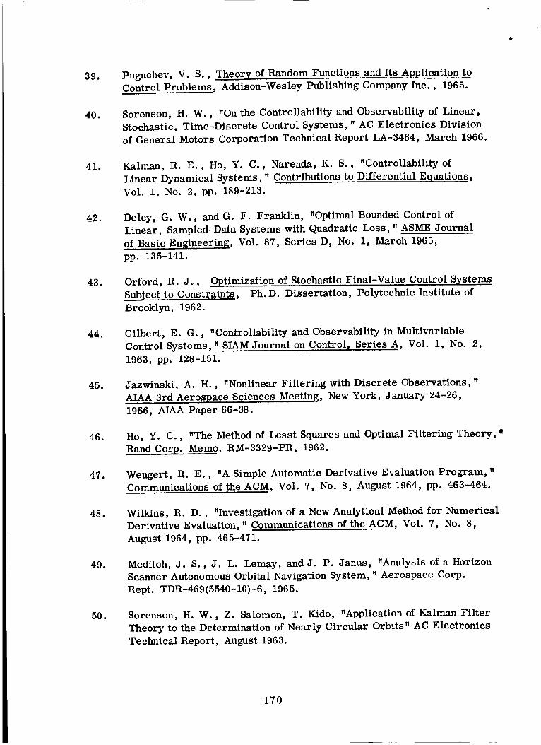
39.
40.
41.
42.
43.
44.
45.
46.
47.
48.
49.
50.
Pugachev, V. S., Theory of Random Functions and Its Application to
Control Problems, Addison-Wesley Publishing Company Inc., 1965.
Sorenson, H. W., "On the Controllability and Observability of Linear,
Stochastic, Time-Discrete Control Systems, n AC Electronics Division
of General Motors Corporation Technical Report LA-3464, March 1966.
Kalman, R. E., Ho, Y. C., Narenda, K. S., "Controllability of
Linear Dynamical Systems, " Contributions to Differential Equations,
Vol. 1, No. 2, pp. 189-213.
Deley, G. W., and G. F. Franklin, "Optimal Bounded Control of
Linear, Sampled-Data Systems with Quadratic Loss, " ASME Journal
of Basic Engineering, Vol. 87, Series D, No. 1, March 1965,
pp. 135-141.
Orford, R. J., Optimization of Stochastic Final-Value Control Systems
Subject to Constraints, Ph.D. Dissertation, Polytechnic Institute of
Brooklyn, 1962.
Gilbert, E. G., nControllability and Observability in Multivariable
Control Systems, " SIAM Journal on Control, Series A, Vol. 1, No. 2,
1963, pp. 128-151.
Jazwinski, A. H., _Nonlinear Filtering with Discrete Observations,
AIAA 3rd Aerospace Sciences Meeting, New York, January 24-26,
1966, AIAA Paper 66-38.
Ho, Y. C., "The Method of Least Squares and Optimal Filtering Theory, "
Rand Corp. Memo. RM-3329-PR, 1962.
Wengert, R. E., "A Simple Automatic Derivative Evaluation Program, "
Communications of the ACM, Vol. 7, No. 8, August 1964, pp. 463-464.
Wilkins, R. D., "Investigation of a New Analytical Method for Numerical
Derivative Evaluation," Communications of the ACM, Vol. 7, No. 8,
August 1964, pp. 465-471.
Meditch, J. S., J. L. Lemay, and J. P. Janus, "Analysis of a Horizon
Scanner Autonomous Orbital Navigation System," Aerospace Corp.
Rept. TDR-469(5540-10)-6, 1965.
Sorenson, H. W., Z. Salomon, T. Kido, "Application of Kalman Filter
Theory to the Determination of Nearly Circular Orbits" AC Electronics
Technical Report, August 1963.
170

51.
52.
53.
54.
55.
56.
57.
58.
59.
60.
61.
62.
Smith, G. L., S. F. Schmidt, L. A. McGee, "Application of
Statistical Filter Theory to the Optimal Estimation of Position and
Velocity on Board a Circumlunar Vehicle, " NASA TR-R-135, 1962.
Friedlander, A. L., A Midcourse Guidance Procedure for Electrically
Propelled Interplanetary. Spacecraft, M.S. Thesis, Case Institute
of Technology, 1963.
Dusek, H. M., "Theory of Error Compensation in Astro-Inertial
Guidance Systems for Low-thrust Space Missions, " Progres in
Astronautics and Aeronautics, Vol. 13, Academic Press, 1964.
Mendelsohn, J., W. O'Dwyer, and A. Kaerchner, "A Numerical
Comparison of Two Orbit Determination Methods," Transactions of
the Ninth Symposium of Ballistic Missiles, Vol. 1, DDC, 1964.
Danby, J. M. A., "Matrix Methods in the Calculation and Analysis of
Orbits," AIAA Journal, Vol. 2, No. 1, January 1964.
Spragins, J. D. (Jr.), "Reproducing Distributions for Machine Learning,"
Stanford Electronics Laboratories, Systems Theory Laboratory Techni-
cal Report No. 6103-7, November 1963.
Stratonovich, R. L., "Topics in the Theory of Random Noise, Volume I,"
(Revised English Edition, Translated from the Russian by R. A. Silverman),
Gordon and Beach Science Publishers, Inc., New York, 1963.
Kuznetsov, P. I., R. L. Stratonovich, and V. I. Tikhonov, "Quasi-
Moment Functions in the Theory of Random Processes, " Theory of
Probability and Its Application, Vol. 5, No. 1, 1960, pp. 80-97.
Friedman, B., Principles and Techniques of Applied Mathematics,
Wiley, 1956.
Moulton, F. R., Celestial Mechanics, The Macmillan Company,
15th Printing, 1962.
Kahn, H., "Applications of Monte Carlo," Rand Corporation Research
Memorandum, RM-1237-AEC, April 1954.
Kuznetsov, P. I., R. L. Stratonovich, and V. I. Tikhonov, Nonlinear
Transformations of Stochastic Processes (Translation Edited by
J. Wise and D. C. Cooper), Pergamon Press, London, 1965.
171

63. Clarke, V. C. (Jr.), nConstants and Related Data for Use in Trajectory
Calculations as Adopted by the Ad Hoc NASA Standard Constant Com-
mittee, n J.P.L. Technical Report, No. 32-604, March 1964.
172

APPENDIX A
GAUSSIAN A POSTERIORI DENSITY FUNCTION
Let the state be n-dimensional and suppose that m measurements are
available at each sampling time.
to the relationship
The conditional density evolves according
where
and
p /zk_1) (A.I)
k-i
P(_Xk/[ ) =/zk-
]'P(._xk_1 _ 1)P(_.x._/_k_l)dX_k_1
k-i /zk-I zpz(._kl_): .pp(_.x__ )PZ(.z.kl%)dx_k
The initial density p X(Xo/Z.o) is determined from
Pz(._o/X)P x(__o )
px(._o/%): .Fpz(.%/xo)Px(_x.o)dx__,_(A.2)
The conditions that the plant and measurement equations must satisfy
so that p(K_k/Z__ can be represented by
1 ^ T-1p(__/zk) = kk exp _ [(__ ._k)] (A. 3)- -%)Pk-1%-
shall be determined.
The initial state and the measurement and plant noise are assumed to
have gaussian distributions.
i [% a )TMolx_o )] (A.4)px(.Xo) = k oexp-_ -_ -a
173
p_ = kwexp-_[ Q ] (A. 5)
pv%) = k exp-_[ R ]Y(A.6)
First, determine the density p X_o/Z_o). Since the measurement noise is
additive, it follows that
p%/_o) = kve_ - _ _% - (A. 7)
Expand h in a Taylor series• It can be written as"0
1
_%1 = h_o_*o>+Ho6X_o+_% (A.71
where
H0
Df
Df
8h10
v-_x1 " • •0
8h nO
8X 1 "..0
6 xTj 15 x"o o --_
5 xTj25 x-'_ O "-O
5 xTjm6 x_ O _
m
Oh10
a_o
8h nO
a_o
174

The ji are defined asO
ji Df=0
The superscript on the hO
82h i 82h iO ... O
aXlaX 1 8XlSX
a2hi a2hiO ... O
%XnSX 1 ax 8xn n
is used to designate the i th component of the vector
h •
"O
Using the expansion in (A. 7) and keeping only the quadratic terms, the
p z(z.u/Xo ) becomes
pz(_z/x) = k exp- 1 T o16Zv _ [6 R - 25zTR-IH 6x--O O O --O
zTR -1+6xTHTR-IH-oo o o6X-o-6--o o _o ]
The term involving rl must be rewritten in terms of 5 x . Let--O --O
Df= R-15z
Y-o o -o
Thenm
_oY'u = [6xTj16X-oo -o'"6 J 6x] Yo
m
i=l
m
Yo
m
6x T i i"-o ( _JoYo
i=i
)6x"-0
175
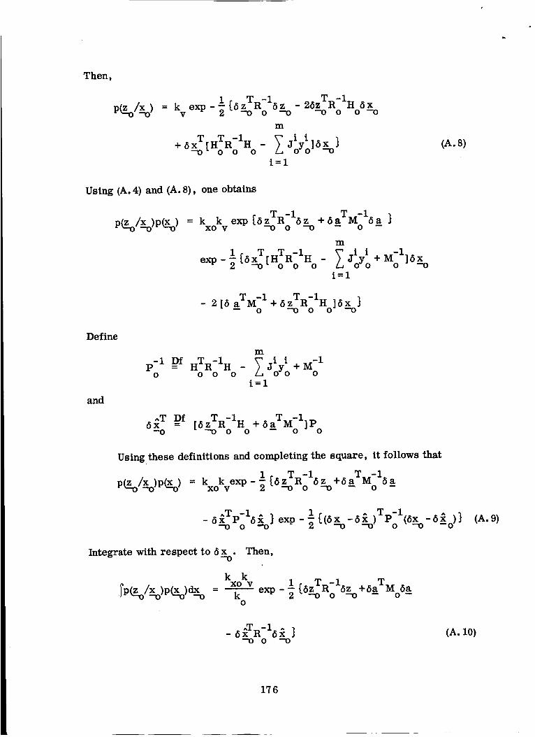
Then,
= k exp--[6 R z - 6xV _- "0 "0 0 0 -'0
m
_ ji i,_+ 6xT[HTR-1H _ oYoj°x-o}
"-0 0 0 0
i=1
(A. 8)
Using (A. 4) and (A. 8), one obtains
exp - _
m
JJoi=1
-2[5_aTM -lo +SgRolHo ]6x]
Define
m
Z ii M-1p-1 =Dr HTR-1H _ J oYo+0 0 0 0 0
i=1
and
6_T Df= _ :lHo aTM-1-o [5 R + 6 ]P-- O 0
Using these definitions and completing the square, it follows that
p z_/x)p%) = k k exp- 1 aTM-16xo v _ [6zTR-16z +6 a-'O O --O " O --
- 6 xTp-15 _ } exp - 1 l(6xu-'o o -o _ [(fix_o-6x_u)TP: -6X_*o)] (A. 9)
Integrate with respect to 5._o. Then,
,_Pz(__o/X)Px(.X,.o)__.u
k k
_ xo v 1 g 15zk exp-7[6 R: +6aTM 6a0
0
_ }-'o 0 -'0
(A.ZO)
176

where k0
is the normalization constant.
ko = [ (2E)n(det Po ) ] -1/2
From (A. 2), (A. 9) and (A. 10), one sees that
1 __u)TPol(5 x __.o)]pX(Xo/Z ) = k oexp-_[6x-6 -6
This can be rewritten as
p%/_) = koe_P-_[%-%) vo %-
where
= x*+6_-'O -'O "-O
The density has the desired form at t .o
Assume at tk that
i ^ T -I
- %_ Pk_% _%_
_, /zk+l.Now, derive pt._ 1 _ • First, form
p%+1/%)= k e_ - 1[%+1 T -iw : -_+9 % %: - _+: >}
Assume a nominal _ and let
Expand f-k+l
in 6Xk
(A. 11)
(A. 12)
(A. 13)
(A. 14)
:k+i= _+imP
in a Taylor series about _ and retain only second order terms
177
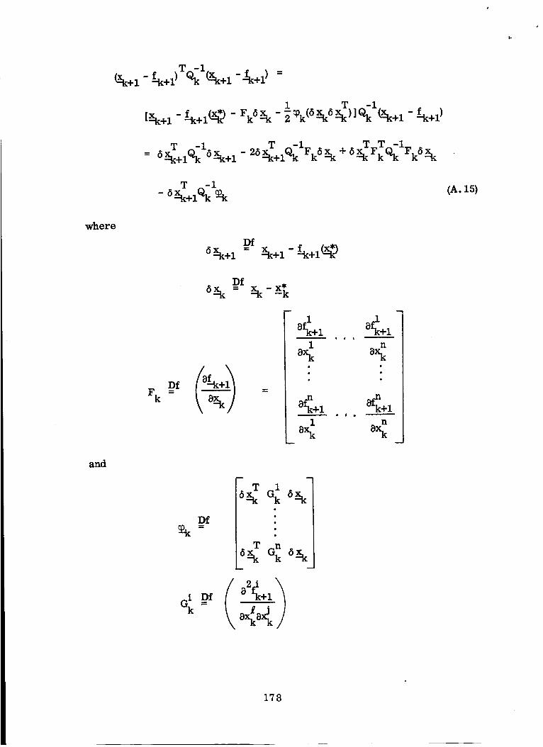
_ f T -1_+_ _+_ % %+_-&+_--
%+1_ %+1
6 T _-i- _+1% (A. 15)
where
Df
6_k+l = _+i - &+_t_
and
Df
F k =
Df
1
1a_
i DfG k =
I M
1 6x k5_ G k
n
_ Qk 6%
• # •
178

For the moment, let
-- +1
Then, it can easily be shown that
n
T -1
i=l
Using (A. 13) through (A. 15), we obtain
1 T -ip(x:k/z_P(Xk+l/Xk) = kkk w exp _ [6- _+1% 6%+i
Let
n
exp - _ - +
i=1
- + 6 ^Tp-i-9"[6_+1%1Fk /!k k ]6%]
n
Bkl =Dr FkQklFk - Z Gk wi+ Pk 1
i=l
= [6_+iQk Yk+5 P
By completing the square, (A. 16) becomes
p_/!Sp_+/%_= kkkw
(A. 16)
e_-E _+i - -
exp - '_{(6Xk _k
179
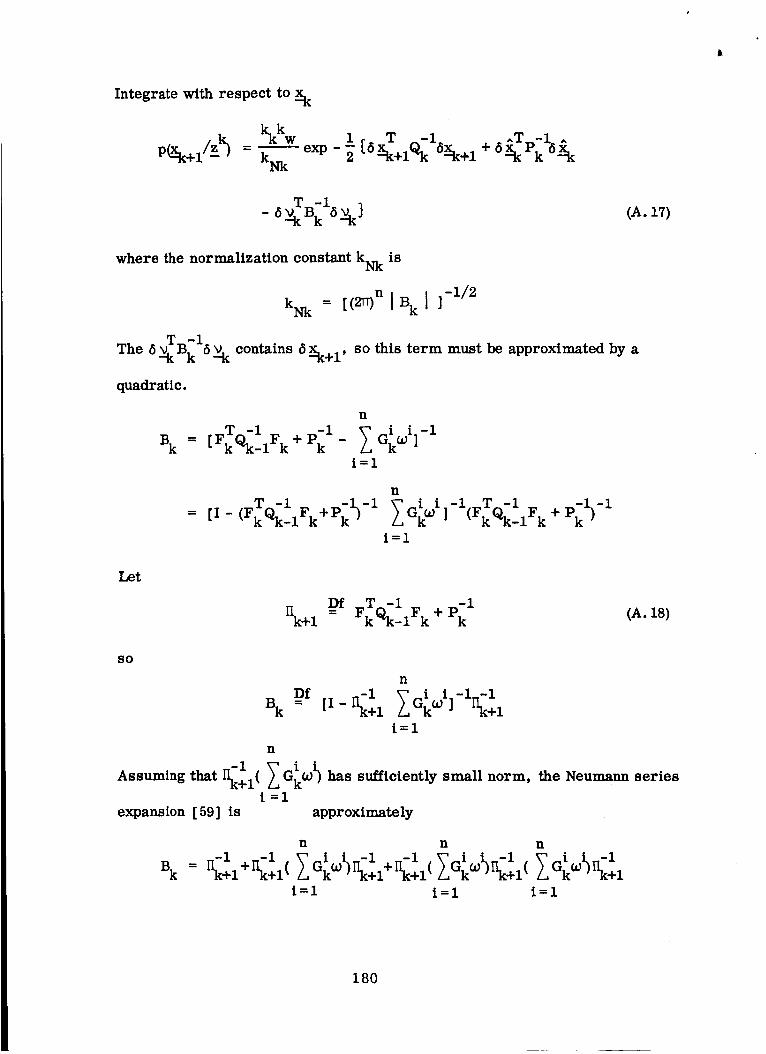
Integrate with respect to _k
kkkw
kNk
1 T -iexp - 7 {6Xk+lQk 6Xk+l
-__
where the normalization constant kNk is
kNk = [(2TT)n IB k i ]
The 6_BklSy.k contains _k+l'
quadratic.
-1/2
so this term must be approximated by a
n
T-1 - _i i.-1Bk [ Fk Qk- iFk + Pk I Z= _ LikO0 J
i=l
(A. 17)
n
Z " -__-_ _a_-_Gk00 ] (FkQk_IF k +=t,-(,_Qa__,,_+_;5-*i=l
Let
Df T -i -i
[Ik+l = FkQk-iFk + Pk (A. 18)
SO
n
v _ i i-i-I
t=1
n
-1Assuming that IIk+ 1( Z Gk OOi)has sufficiently small
i=1expansion [ 59] is approximately
norm, the Neumann series
Bk =
n n n-1 -1 i " -1 -1 i " -1 _i i--1
i=l i=l i=l
180
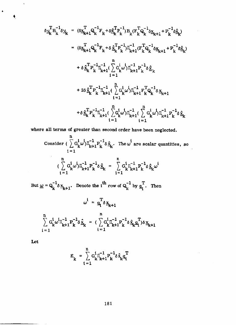
_L
= _% k )_-_( k% 6%+_
n
._,-_ -_ _ -_ -_ .+_ k_÷_(Z%__ _x_i=l
n^T -i -i i " -i T -i
i=l
n n
^T -i -i i " -i G i i -i p-i ^
i=l i=l
where all terms of greater than second order have been neglected.
n
i -i -IConsider ( ZGk_k;iPk 6&.
i=l
The i are scalar quantities, so
n n
Z.a
i=l i=l
_16Xk÷l. Denote the i th _1 TBut _ = row of by _i " Then
n
i i-i -iUk(_ Hk+IP k 6&
i=1
n
i_-i p-i ^ T
i=l
Let
E k
n
Z i -i -i
i=l
181

Then
_kPk_k+Pk6%
^T-i-i T-_ ^T-i-i+ [25_P k Rk+IFkQ k +6Y_kP k Rk+iEk]6_k+l
T -i -i T -i T -i F -I+ET -i E+62_k+l[Q k FkRk_IFkQ k +2EkRk_ I kQk kRk_l k]6Xk÷l (A. 19)
The introduction of (A. 19) into (A. 17) gives
i T -i -i -i T -i T -i -i T -IexP-216%÷l[Qk -Qk FkRk+iFk% - 2ZkRk+iFkQk -ZkRk+iZk]6%÷l
26_TP-I--IF -i i- _k k I_(+1[ kQk ÷2Zk]6Y_k÷l} (A.20)
The density pZ_k+i/Xk÷1) is
i T -i
p z_k+l/Xk+l ) = kvexp - 2 [Z_k÷l-_k÷l) Rk+l Z_k÷1 - _k÷l )_
Following the procedure used for pz(_/Xo), this becomes
i T -i
pz(9.k+i/Ytk+l)= k exp _ [5v - %+iRk_ _k+1}
I. T T R-Iexp -_ _6Y_k+l[Ilk+I k+iHk+l -
T -i-26%+iRk£1Hk+16_k+1]
m
ji i ,k+lYk+l] 5_k+l
i=l
(A.2i)
182

Then, one sees that
kNk
1 T -i
exp - _ [6 z.k+lRk+l 6_'k+l
^T -i -i -i -i ^
+ 6/_k(Pk - Pk Rk+iPk )5_k]
1 T -i _ -exp- _ [6%+iPk+lSXk+l 25_+iPk+llS/_k+l } (A. 22)
where
-1 Df Q_I -1 F -1 F T -1 T -1 -1 ET_-I EPk+l = -Qk kKk+l k% -2ZkKk+lFkQk - kllk+l k
m
T -1 i l- Jk+lYk+l
t--1
^T Df ^T -i -i F -i+i E T -i5_k+1 = [6/_kPk Ilk+l( kQk 2 k )+5"_k+iRk+lI'Ik+l]Pk+l
Completing the square and integrating with respect to 5 _k+l gives
p%+d'--5 kkkkvkk+_kNkexp-_{6%+1Rk;16%+1
^T -i -i-i -i ^ ^T p-i .,,+5/_k(Pk -Pk Rk_'lPk )5/_k- 5/_k+1 k+10/_k+l J (A.23)
where
kk+l = [ (211)n I Pk + i I ]
Division of (A. 22) by (A. 23) yields p(___+l/k+_.
-1/2
i ^ Tp-i ^= kk+lexP-_[(5/f_k+l-5!!k+1) k+l(5/f_k+l-5/f_k+l)}
1. ^ Tp-i ^: kk+lexp- 7 t(-.Xk+l-/!k+1) k+l(-Xk+l- !£k+1)] (A. 24)
183

PRECED]1QG P_K_E BLANK NOT FILM IED.
APPENDIX B
MATHEMATICAL MODEL FOR THE SPACE NAVIGATION PROBLEM
The digital computer program utilized for the study presented in
Chapter 5 has been developed by the AC Electronics Division of General Motors
Corporation to investigate the general problem of guidance and navigation for
interplanetary space vehicles. In this appendix, the general equations that
are relevant to the problem of Chapter 5 shall be stated with a minimum of
accompanying discussion.
The motion of the spacecraft has been assumed to occur about a single
central body as described by (5.1), so analytical solutions of the equations
are possible. Thus, the position and velocity at any sampling time are
obtained from explicit analytical expressions rather than by numerical inte-
gration. These expressions are well-known [60].
For this model, it is possible to obtain explicit expressions for the state
transition matrix appearing in (5.6) [55].
Let
When the nominal is contained in the X-Y plane, the _i have the form
1 L '15:1L °1: 2 r:i:,51 ; =
0 _33 0 _36
(B. I)
185

_3[_41 _42 0
--j° i oL o 0 _63
_4 = _54 _55
0 0 _66
Let the eccentric anomaly at tk be Ek and let the eccentricity and mean
angular rate be e and n. Define Sk and Ck as
sinE k = Sk ; cosE k = Ck
Then, the elements of the submatrices are
= 1 [ C2(l+e_e 2)_11 (l_e)2(l_e Ck )
+ Ck(2+e+2e2-e3 )
-2- 5e+2e 2+3EkSk]
0i= A-7 r(l-e)(l-e Ck) Sk (l-Ck)
_21
Jl - e 2
(1-e)2(l-e CQ[SkCk(l+e) + Sk(2-e) - 3EkCk]
= i [Ck2 + Ck(-l-2e+e2 ) + i]_22 (l-e)(l-e Ck)
(Ck - e)
_33 - (l-e)
_i4 = (i-e) Sk + 2]n(1-e Ck) [-Ck(l+e)
_i -.e2 [Ck(2_e)_15 = (l-e)n(l-e Ck) + 2Ck(l+e ) - 4 - e + 3EkSk]
186

2
t25 = _ 1n(1-e Ok--_ [SkCk(2+e+e2 ) + 2Sk
Sk(1-e )
n
(l-e) 2(1.e Ok) 3
(1-e) (1-e Ck) 3
+ 8kO,k(-2.Se+2e5
+ 8k (l"l'e+3e2-e 5 + 3Ek (Ck_e)J
_51 = ._-e
(1-e)2(1-eck)-3
_52nS.
(l-e) (1-e Ck,) 3
+ C/_(,?,+Se) - Ck (l+e)
- 1 - 3e + e 2+ 3EkSk]
EeC_- ,.Ck ÷_÷._ 2j
<}44= _ [Ck('e+e'?') 2C_(I-/-e)+ ?Ck +1-e](1-e Cl_a
(1-e)(i-e Ck,)3 - SkCk(',_-e )
187

Sk%/1-_---_ 2_ 2C k +2-e]- [e Ck(1-e Ck)3
_55(1-e Ck)3
[-C3(2e+e2+e 3) + C2(4+5e+5e 2)
-Ck(l+3e ) - 2 - 3e - e 2 + 3(l+e)EkSk]
(l-e) Ck
_66 - (1-e Ck)
The computation of the transition matrix is carried out in an in-plane
cartesian coordinate system and then transformed using a rotation matrix
into the basic nonrotating cartesian system. The evaluation of the two body
equations and the transition matrix equations provides the nominal and actual
trajectories and the linear model.
A horizon sensor has been assumed to be available to provide data for
navigation purposes. This instrument provides a measurement of the direction
of the line of sight to the center of a reference body relative to a nonrotating
reference frame and a measurement of the angle subtended by the reference
body. These angles are depicted in Figure B-1.
These measurements are described by the three angles, _, 5, and _.
The local vertical is defined by the elevation angle _ and the azimuth angle 6.
The _ is defined to be positive when the vehicle is below the X-Y plane and 6
is measured counterclockwise from the X axis.
X 3-- - -1 (B.--2)
188

Earth
Center
Z
Vehicle
L
v
Figure B-1. Geometry of Angular Measurements
X
r xsin-1 2
-1• COS
X 1
where
9. 9._ y2_ 1/2R = (XI+X 2 ...3,
The subtended angle fi is given by
(B-3)
where
r-1 o
= sin _- (B-4)
r = radius of reference body.O
Both the first and second order partial derivatives are required for the
navigation procedure. The first order observation matrix Hk is, in general,
189

More specifically, this can be written as
H k =
m
0a__q._ aa__q__ a___q__
8X 1 8X 2 8x 3
8X I
06 86
8X 2 8X 3
8X 2 8X 3
0 0 0
0 0 0
0 0 0
(B-5)
where the derivatives taken with respect to the velocity components of the state
vector (i. e., X 4, X 5, X 6) are identically zero as indicated. Denote the non-
zero submatrix as Hl(t Q.
-sin a cos 6
It follows that
-sin _ sin 6 2+ 1/2--(X 1
R R R 2
2-sin 2 6 cos 6 0
X 2 X 1
-X 1 tan/3 -X 2 tan/3 -X 3 tan
Next, let
R 2 R 2 R 2
1Jk
(B.-6)
190

where
2ay
32y
8XlSX 2
28y
8XlaX 6
28y
8X28X 1
28y
eeoeeeeeeeeeo=eeeeooeoe
28y
8X6X 1
28y
2ay
There is no dependence upon velocity, so the partial derivatives relative to
velocity components are identically zero.
isubmatrix by Jl(tk) (i = 1, 2, 3). Then,
m
j111
1Jk(tk) = J21
u31
1 1
J12 J13
1 1
J22 J23
j1 T132 u33
Denote the upper left-hand (3x3)
(B-7)
1
Jll
-sinX 2
[sin25 - 2--1R 2 ]
1J12
X 2 sin _ cos 5
R
sin26[2___R2 + 2
X 2
1J13 = cos5 (1-2sin 2_)
R 2
1
J21
X 2 sin _ cos 5
R2 +
[ R 2
sin 2 5
2X2
191
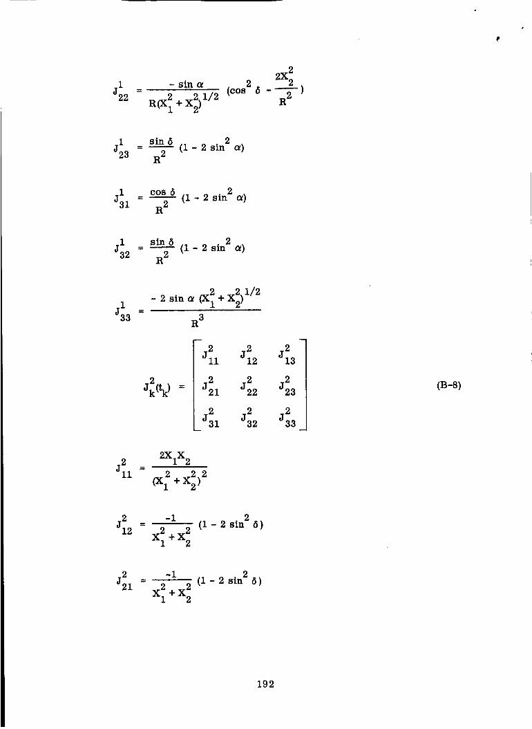
1J22
- sin(cos 2 5 -
2
2X 2
R 2 )
1J23
sin5 (i- 2 sin2 _)
R 2
1
J31cos 6 (1-2 sin 2 u)
R 2
jl32
_ sin6 (1 - 2 sin 2 _)R 2
1J33
2 _ i/2- 2 sin_ (XI+X )
R 3
2
Jll
2= J21
2J31
2J12
j222
2J32
2J13
2J23
2
J33
(B-8)
j211
2XIX 2
2 2)2(XI + X 2
2J12
-1
2 +X_X 1
(1 - 2 sin 2 5)
2J21
-1m
2+ 2X 1 X 2
(1 - 2 sin 2 5)
192

2
J22
-2XIX 2
2 2 2 2 2J31 = 0 = J32 = J33 = J13 = J23
Jk(tk )
-3
Jll
3= J21
3
J31
3 3-J12 J13
3 3J22 J23
3 3J32 J33
(B-9)
3 - tan t3 (1Jll = R 2
2 2X 1 tan 2 _ 2)[ 1
r 2 R 2 )0
XlX 2 tanj3 =
12 R 22 +r0
XIX 3 tanj3 _
13 R 2
9.( tan2 r_ ÷ )
12 _"O
X1X 2 tan3J21 -
R 2
÷ 2( r2 R-2)
0
3 - tan/3 (1J22 = R 2
2tan2_ 2X_X 2
2 R2ro
3J23
X2X 3 tan
R 2
2
ro
193

3 XlX3tan_ (tan_22J31 - R 2 r
O
X2X3tanj3 _
32 R 2 (R--2+ 2ro
3 -tan (1J33 = R 2
Note that the ffil(t _ are symmetric.
2 2X 2X 3 tan 2/3 - 3)
r 2 R 20
The preceding equations provide the complete model for the system. To
accomplish the Monte Carlo simulation, the actual trajectory of the spacecraft
is computed in addition to the nominal trajectory. The initial deviation of the
ensemble with mean zero and covariance matrix M (see (3.3)) is selectedO
using a gaussian random number generator [61].
It is the state of the actual trajectory that is to be estimated. The
measurement data are computed from the nominal and actual trajectories. The
exact measurement values are corrupted by adding at each time numbers from
a gaussian random number generator assuming the ensemble has mean zero
and covariance matrix R k.
194

APPENDIX C
GRAM-CHARUER AND EDGEWORTH EXPANSIONS
The Gram-Charlier and Edgeworth [10,23, 39] expansions have been
utilized in Chapter 6 to approximate the a posteriori density function P(Xk/Z _.
The purpose of this appendix is to discuss these expansions and to demonstrate
by example the nature of the approximation of various truncations to some
well-known density functions.
C. 1 FORMAL DEVELOPMENT OF THE GRAM-CHARLIER EXPANSION
Consider a random variable _ with a known density function and let x
be the normalized random variable
_-mX --
The m and a are the mean and standard deviation associated with _. Denote
the density function for x by f(x) and let *(x) represent the gausstan density
function with mean zero and unit variance.
Consider an expansion of f(x) having the form
C
f(x)= Co*(X)+ Cl,'(x)+ T.,2,"(x)+ ... (c.i)
where ,(k)(x)is the kth derivative of , and the ck are the constants. The
derivatives ,(k)are related to the Hermite polynomials according to [i0]
2
t_'d_ne -x2/2 = (-1)nHn(x)e-X /2 (C. 2)
The Hermite polynomials satisfy the orthogonality condition
tz'l mn 2/2dx <i Jr Hm,..,-- n! form n4-_ (x)e-X = = (c.3)0 for m _ n
195
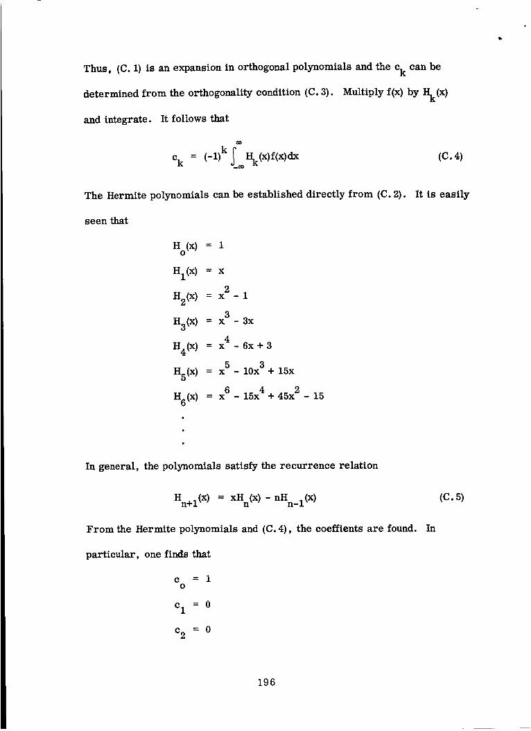
Thus, (C. 1) is an expansion in orthogonal polynomials and the ck
determined from the orthogonality condition (C. 3).
and integrate. Itfollows that
ck = (-l)k_o Hk(x)f(x)dx
can be
Multiply f(x) by Hk(X )
(C. 4)
The Hermite polynomials can be established directly from (C. 2).
seen that
H (x) = 10
HI(X ) = x
2
H2(x ) = x -1
3H3(x ) = x - 3x
4
H4(x ) = x -6x+3
5 _ 10x 3 + 15xH5(x) = x
6_ 15x 4+45x 2_ 15H6(x ) =x
In general, the polynomials satisfy the recurrence relation
It is easily
Hn+l(X ) = XHn(X)- nHn_l(X)
From the Hermite polynomials and (C. 4), the coeffients are found.
particular, one finds that
C = 1O
Cl = 0
c2 =0
(c. 5)
In
196
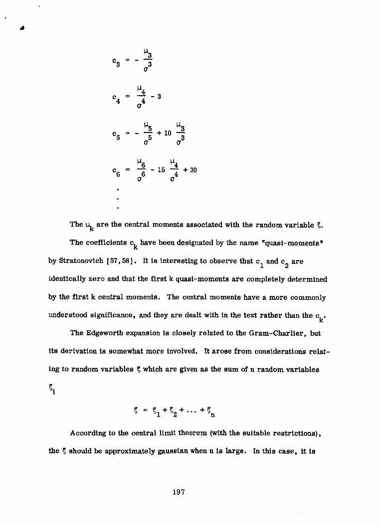
_3
C3 = - "-'_"G
c4 = --4 -3(T
_5 kz3
c5 = - 5 + 10 3O" Cr
c6 - 6 - 15 -_G G
+ 30
The _k
The coefficients ck
by Stratonovtch [ 57,58 ].
are the central moments associated with the random variable _.
have been designated by the name "quasi-moments"
It is interesting to observe that c I and c2 are
identically zero and that the first k quasi-moments are completely determined
by the first k central moments. The central moments have a more commonly
understood significance, and they are dealt with in the text rather than the ck.
The Edgeworth expansion is closely related to the Gram-Charlier, but
its derivation is somewhat more involved. It arose from considerations relat-
ing to random variables _ which are given as the sum of n random variables
= _1+_2 +''" +_n
According to the central limit theorem (with the suitable restrictions),
the _ should be approximately gaussian when n is large. In this case, tt is
197

desirable that all terms of the same order in n be included when the expansion
is truncated. It was found that under this constraint, the expansion for the
normalized variable x is
f(x) = ,(x)
1 c3,(3) (x)+ 3!
1 + 10 c23,(6)(x)+ c4'(4)(x)
1 35 280 c33¢(9)+ _.v c5'(5)(x) +_-.v c3c4_/(7)(x) +-_".v (x)
+ .... (C.6)
where terms of the same order in n are stated on the same line. The details
regarding the derivation of (C. 6) shall be omitted.
The Gram-Charlier and Edgeworth expansions can be written in terms
of the characteristic functions of f(x) and ,(x). Let _0(s) be the characteristic
function of f(x)
o(s) = ®eiSXf(x)dx
The Fourier transform of the derivative of a gaussian density is given by
ffeiSX_(k)(x)dx = (-is)ke -s2/2 , k=O,1,...
so the Gram-Charlier expansion becomes
m
-s2/211 c3 c4c_(s)= e +_., (-is)3+_ (-is)4+...]
(C. 7)
(c.8)
198

C. 2 APPROXIMATION OF DENSITIES USING THE EXPANSIONS
In this section we attempt to approximate densities that are distinctly
nongaussian in order to examine the effects of various truncations of the
expansions. First, consider a uniform distribution
p(g) = 12_ha-h_a+h
Lo elsewhere
The moments of this distribution are known to be
m = a
cr2 = h2/3
_3 = 0 = _5
-- h%
_6 = h6/v
We shall only consider truncations of the expansions that contain at most the
first six moments.
The density for the normalized variable is
( __L_I - d-_'_ _j-_"f(x) = z4-g' x
0 elsewhere
This density is symmetric about the mean, so the Gram-Charlier and Edgeworth
expansions are identical through the sixth order moments. We shall consider
the following approximations to f(x).
Case 1: f(x) = _(x)
199
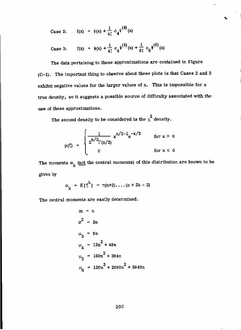
1 c4_(4)Case 2: f(x) = _(x) +_. (x)
1Case 3: f(x) = _(x)+_.v c45(4)(x)+ _,vc6'(6)(x)
The data pertaining to these approximations are contained in Figure
(C-I). The important thing to observe about these plots is that Cases 2 and 3
exhibitnegative values for the larger values of x. This is impossible for a
true density, so itsuggests a posslble source of difficultyassociated with the
use of these approximations.
2The second density to be considered is the X density.
i n/2-1e-X/2 for x > 0p(_) = 2n/2r(n/2)
0 forx< 0
The moments c_k _ the central moments) of this distribution are known to be
given by
olk = E[_k] = "rl(n+2) .... (n+2k-2)
The central moments are easily determined.
m=n
2 = 2n
_3 = 8n
_4 = 12n2 + 48n
_5 = 160n2 + 384n
_6 = 120n3 + 2080n2 + 3840n
2OO

The density for the associated normalized variable x is
_x+n
" 12n)1/2 (_/-2_ x +n)n/2-1e 2f(x) = 2n/2I'(n/2)
L °This density is approximated for two values of n.
the results for n = 1 and Figure C-3 depicts the approximations for n = 4.
These cases are plotted in each of these figures.
1 c3_/(3)(x)Case 1: f(x) = _(x) + 3--
1Case 2: f(x) = _/(x) + 3"-_c3 _/(3)(x) +_._ c4 _(4)(x)
1 c3_(3)(x) _.tc4_/(4)(x)Case 3: f(x) = _(x) +_.T + +
x> -(n/2) 1/2
x < - (n/2) 1/2
Figure C-2 contains
The latter two have been included because they illustrate the differences
between the approximations provided by the Gram-Charlier and by Edgeworth
expansions. Both of these cases include the fourth order moments, but no
moments of higher order. The Edgeworth expansion is seen to provide a
significantly better approximation in each case.
201

¢) ¢)
III
I I
o.
Q)
• \ _ ° .
!
!
m I
0
0
0*p.I
*r..l
.r..l
I
202

q) _ q)_o _ no
cd cd
S
//
/f
!
203
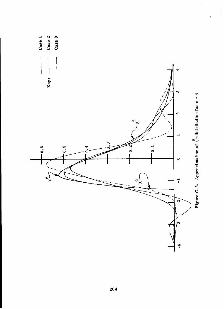
/J
//
204

APPENDIX D
DERIVATION OF NONGAUSSIAN A POSTERIORI DENSITY FUNCTION
In this appendix equations defining the moments of the most general
a posteriori density function considered in this investigation are derived.
Attention is restricted to scalar plant and measurement equations. The
techniques used in the derivation can be applied to more general density
functions and/or more general system equations (including multidimensional
systems). Increased generality leads only to algebraic difficulties, not con-
ceptual difficulties.
Suppose that the plant and measurement equations are described by
2xk = fkXk_l + gkXk_1 + Wk_ 1 (D. i)
zk --hk_k+ek_+vk (D.2)
where the additive noise [wk] and Ivk] are white, gaussian sequences. The
initial state x is also gaussian. The system (D. 1) and (D. 2) can be consideredO
to represent the second-order Taylor series expansion of some more general
nonlinear system.
sampling time by
p(_/z k)
where
The a posteriori density shall be approximated at each
kk exp _ 1 2 1 1= _ _k[I+_c3H3¢_)+_.,%H4(_
102. _,+ _.Tc3n6(_,k) ] (D. 3)
_k-Pk
205

C3 =---_
Pk
'_k
c4 - 4 - 3
Pk
and
H3(_k) =_3k_3_k
4. 6 2H4(_ =_ k _k + 3
H6(_k) =_k- 15_ +45_k- 1
2The xk is the mean value and Pk' _k' Vk are the second, third, and
fourth central moments of P(Xk/Z _. Relations defining the moments are
derived below. In the derivation, use is made of general relations between
the moments and central moments of a distribution and also of the special
properties of the moments of a gausstan distribution. Relationships of this
nature are summarized in Appendix E.
D. 1 INITIAL SAMPLING TIME
Since the x is assumed to be gaussian and since a measurement z isO O
assumed to be available, the initial sampling time is a special case of the
more general results presented in Section D. 3. According to (2.15)
P(Xo/Zo) = P(Zo/Xo)P(Xo)
J'p(zo/Xo)p (Xo)dx°
206

From (D. 2), it is true that
k1 (Zo - hoXo - ex2)2
exp - 2r
o
21 (Zo - hoXo)
= kv exp - _ 2r
o
21 (-2e zxO0 0
exp - _'
x 3 2 4e ÷+2ho o o eoXo)
2r
o
It is necessary to approximate the second exponential. Let
2ez he e
I_ oo 2 oo 3 o 42 x -_x -_xB(x°) - r r 2r 2o 2 o o
0 0 0
(D. 4)
and let
e zDf o o
b2 - 2r
0
h eDf o o
b3- --7-r
o
2e
IX ob4 = _--
2r 2O
Before dealing further with the second factor, let us form P(Xo/Zo).
Df 1k t =
O fp(Zo/Xo)P(Xo)dXo
Let
207

Then,
x -a z -hx1 ---o 2 1 o o O)2ex p
P(Xo/Zo) = k'k k exp - _ -m¢-"_---) exp - _ ( 2 B(Xo)OVX 0 r
• o
Combining the two gaussian terms and completing the square, one gets
P(Xo/Z o)
2 ^2
1 a 2 z 1 o_o_ )exp-_(= k'k k exp-_(---_+ 2
ovx m r _ o0 0 o
_°)2exp B(Xo)
where
h21 o 1
2 2 2r m
o o o
h z
2( 020_o = _o _ +-_a2)r m
0 0
and 2The _o o
were linear.
would be the conditional mean and variance if the measurements
The factor exp B(x o) then serves as a correction to the linear
results.
Now, rewrite B(x o) in terms of the variable _o' That is, let
_A÷_A÷_,X'o: _o÷_,Xo-_o)÷_._(Xo-_o)_
+_3_(_o-_o)3+_4_(Xo- _o)4
The values of the fit that satisfy the equality are easily determined to be
_._o ^_o'_Yofll = + 3b3_ +
208

^ ^2821 = b 2 + 3b3_ o + 6b4_ °
A
_31 = b3 + 4b4_o
_41 = b4
The constant _o can be considered separately. Define BI(_ o) as
2 3 4Bl(_o) =Df _1_] ° + _21_ ° + _31rio + _41t]o
where
_o Xo o
Now, let us approximate exp Bl(_o ) by a power series. Then,
1. Sl(rlo) ]2 3exp BI(_o) = 1 + BI(_o) + 21 [ + °[BI(_o)]
Terms of greater than second order shall be neglected. Let
B2(_o) Df 1 ]2= _[B!(r_ o)
2 3 4 5 6 7= /_22rlo + _32r]o + _42r]o + _5r]o + _6_o + _7r]o
where
_22 = ,8 /2
Df_32 = _1_21
Df 2= ( 21
Df
+ 2 i 3 )/2
(D. 5)
209

_6 Df= (/331+2 2921fl41)/2
_7 Df= _31/341
Thus,
P(Xo/Zo).- = k'k kovx
1 2 z 2 _2
exp- o o2-2 )m r
o o o
1 rlo. 2
eXPgoeX p - _ (_--) [i +Bl(rlo) +B2(_]o)]o
The constant [k k exp - 1/2 (a /m ° + z /r - /_ )exp 9o ] will be cancelledv x
by the corresponding term in o_P(Zo/Xo)P(Xo)dX o. Define the constant ko to be
ko
2 z 2 _21 a + o o
= k'k k exp-_( ) exp9 °ovx 2 2 2m r
o o o
1 1
=O O
-- J'exp - _ (_--_°)2 [ 1 + Bl(_o)+B2(rlo) ] drlo]O
-1
Note the change of variable for the integration. Thus
1 1k
O 1 + E[B1] + E[B2]
and
1 [4_-_rr exp-_ [i+Bl(_o)P(Xo/Zo) = I+E[BI] +E[B2] o o
+ B2(rlo)] ]
(D.6)
210

The expected value is obviously taken relative to the gaussian density
11,/_:'rr° exp- 112('nolrro)2.
To cause P(Xo/Zo) to assume the form prescribed by (D. 3), determine
the moments E [r_1o/Zo]
^ i ^ i
E [(x° - _o) /Zo] = _(x° - _o)P(Xo/Zo)dX °
i
I E_r_1fE_+_oBi%)1 + E(B1) + E(B2) n°
i 1 _o)2+ _oB2(_o ) ] exp - _ d_o]O
• i E [ _ioB2(r_o ) ]i Z[_o] + E [_oBl(_o) ] += (D.7)
E [_o/Zo] 1 + E[BI] + E[B2]
The expectations indicated in (D. 7) are easily determined.
E[B1] = E[fil,'qo+fi21_2o+fi31_3o+fi41v_4 o]
2= fl21rr ° + 3fl41_
3 4 5 6 7 8E [B2] = E [f122rlo2 + f132rlo + _42rlo + fl5rlo + fl6rlo + _7_o + f18_o ]
= + + ÷
This follows from the fact [10] thatfor a gaussian variable rl°with
mean zero and standard derivation rro
0 , t=1,3,5,...E[_io] =
(t-1) n i , i=2,4,6,...O
211

The E [_oBl(_o ) ] and E [_ B2(_o) ] are determined in the same manner.
The central moments can be determined directly from the E [_o/Zo].
For example,
By definition,
SO
E[no/Z °] = E[(x o- _o)/Zo]
^ /Zolx = E[x °o
= E [Xo/Zol - _o
= _ + E[_o/Zo] (D.8)O O
Thus, the E (_o/Zo) provides a correction to the conditional mean obtained from
the linear density.
But
The variance is determined by considering the second moment.
E[rl2/Zo I = E[(x ° - _o)2/Zo ]
E [[(xO ^ ^ - ^ 2/z O]= _xo)+ (xo _o)]
= E[(Xo - Xo)2/Zo ] + 2E[(Xo - Xo)/Zo ](Xo - _o) + (Xo - _o)
E[Xo-Xo/Zo ] = Xo- _o = 0.
A
o- _o = E[_o/Zo]
and
212

SO
2 Df _o)2/Zo]Po = E [(x° -
= E[T]_/Zo] - E2[_o/Z o] (D. 9)
The third and fourth central moments are found in the same manner and are
given by
_o = E[(Xo - Xo)3/Zo ]
/Z -= E[_]o o] 3E[_]o/Zo]Po2 E3[_o/Z o]
_o = E[(Xo - Xo)4/Zo]
= s[_/Zol-4%zE_o/Zo]-6p2oZ2E_o/-o]-_4[no/,oi
This completes the derivation of the moments for the first sampling time.
D. 2 THE PREDICTION DENSITY P(Xk/zk-1 )
The density P(Xk/zk-1), according to (2.13), is given in general by
p(xk/,k-:fp(xk_/zk
(D. 10)
(D. Ii)
It is necessary to proceed carefully in determining this density.
if one attempts to establish k-1P(Xk/Z ) directly from the formula, it becomes
apparent that one is led to a hopeless morass of algebraic manipulation. On
the other hand, it has been pointed out that the object of the approximation
procedure is to determine the moments of the distribution. That is, it is
In particular,
desired to determine
E[4/zk-1 ] = jxkP(Xkri /zk-1_)dXk (D.12)
213

This can be written as
i- k-i
E [Xk/Z ]
i k-i
: ;xyp%_/_ )p%/xk____ _
Iterating the integrals, this becomes
i- k-1 k-1 iEtxk/_ I : ..TP(Xk_/_')t;j'xkp(xk/xk_l)<'_b/;tds<_l
The innermost integration can be easily accomplished because of the assump-
tions on the plant. Consider the mean value.
2
1 xk - (_xk-1 + gkxk-1) leixl<EtS</___.l : k i'xk exp -'_ [ qk-1
It follows immediately that
Thus,
2
Et_k/xi<-_l : _xk-1 + gks<-i
E [Xk/zk-i ]
k-i
From the definitionof P(Xk_i/z ),
EiXk/zk-li : __l+
Df ,,
: _/k-1
2 k-i: ,f_fkxk-_+gkXk-1)P%-i/_)<5<-1
one obtains immediately
2 ^2
gk(Pk_l + Xk_ I)
Continue in the same manner to determine the higher order moments.
2 2 2 2E[xk/xk-l] : %-1 + (f'kxk-:l.+ gkxk-1)
and so
2. k-i 2E [XklZ ] = qk-i +
(D. 13)
Thus,
2 k-i_E[Xk_l/z I+2_E 3 /k-1 2E 4 /_k-1lXk_1 _4"g k [Xk_1 ]
214
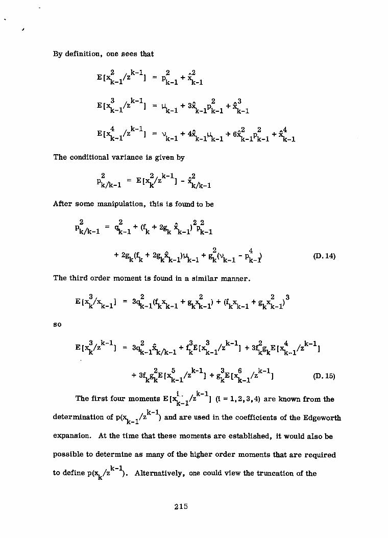
By definition, one sees that
2 • k-1 2 ,,2E[Xk_i/z ] = Pk-i + Xk-I
3 , k-1 ,, 2 <E[Xk-1/z ] = t_k-1 + 3Xk-lPk-1 + -1
4 k-1 ^
E[xk-1/z ] = _k-I + 49'k-1t'Ik-1
The conditional variance is given by
2 = E[x_/zk-l], 9_/k_ 1Pk/k-1
_^2 2 ,,4
+ UXk-lPk-i +-kx-1
After some manipulation, this is found to be
2 2 ,, .22Pk/k-I = qk-i + (fk+ 2gk Xk-l) Pk-i
2 4
+ 2gk(fk + 2gk%-l)_k-i + gk(_k-1 - Pk-_
The third order moment is found in a similar manner.
3, ^2 .
SO
2 2 3+ gkXk_l )+ (fkXk_l + gkXk_l )
(D.14)
3.k-i 2 ^ 3 3 k-1 4 k-IEt_R/" I = 3%_iXk/k_I+_Z[_R_/" I+3{gkZrXk_/Z]
+ . /zk-1[Xk-i/z ] + gk [Xk-1 ] (D. 15)
i.. k-i
The firstfour moments E [Xk_l/Z ] (i= 1,2,3,4) are known from the
determination of P(Xk_l/zk-1 ) and are used in the coefficientsof the Edgeworth
expansion. At the time that these moments are established, itwould also be
possible to determine as many of the higher order moments that are required
to define P(Xk/zk-i ). Alternatively, one could view the truncation of the
215

Edgeworth expansion as implicitly requiring that the higher order moments
be the same as the basic gaussian density. Then,
_5 = _t7 = 0
6
_6 = 5Pk-1
8
_t8 = 7Pk_ 1
This assumption will be used here. Then,
[ 5 /zk-1] = " 10^3 2 ^5xk_I _-i"k-i+i°_-i_k-i+ _k-lPk-1+_-i
6_ = 5Pk_ 1
^4 ^6+15_k_iPk-1+_-1
2" ^5 2 ^7+ __iPk_1+h_-1
[ 8 /zk-ll 8 + 70Xk_l_k_l + 56 _l_k_lE Xk_ I = 7Pk_1 + 140 _ip -i
28 ^6 2 ^8+ Xk_iPk_l + Xk-1
The third central moment is related to the E [x_/z k-l] according to
3- k-i 2 ^3
_k/k-I = E(Xk/Z ) - 3Xklk-lPklk-i- Xklk-i
The analytic expression for the _k/k-i shall be derived for future reference.
It is not necessary since (D. 15), (D. 16) and the relations for the moments
E [X__l/zk-l] can be used to determine _k/k-l"
216

In particular, after considerable manipulation, one finds
2 ^ 4 ^ _^2 2
+3%gk(1_-iPk-1-xk-_k-1-6xk-1%-i-2Pk-i_-2
3 6 + 4 ^2 2 2+gk(Tpk_l33Pk_lxk_l- 3Pk_pk_l-12___pk_1__1
The fourth order moment is determined from
4/EEXkXk-11=3q__l+6(_kxk_1+ 2 2 2 2 4gk_k-1_ qk-1+(_kXk-1+gkXk-1)
Thus,
E (x_/z k-1 )
(D. 17)
4 4 k-1
3 7 k-1 4 8 . k-1+ 4fkgkE (Xk_l/Z ) +gkE(Xk_l/z )
The fourth central moment is determined from E(x_/z k-l)
_^2 2 ^_k/k-1=_.(_l_k-1)_4_/k_1_/k_1__/k_lpk/k_1__Ik-1
(D. 18)
(D. 19)
Equations (D. 18) and (D. 19) serve to define Vk/k-l"
This completes the derivation of P(Xk/zk- _. Recall that the only approxt-
mation is in the number of terms retained in the expansion and in the moments
of greater than fourth order.
217

D.3 THE GENEP_LRELATION FOR P(Xk/Zk)
The general relations for the moments of P(Xk/Z _ are derived in a
k-1manner similar to that utilized in Section D. 1. The density P(Xk/Z ) has the
form given by (D. 3) rather than the gaussian P(Xo), so the derivation is some-
what more complicated algebraically.
Let
According to (IV), the P(Xk/Z_ is described by
P(Xk/zk-1) p(zk/xk)
p(zk/zk-1 )
Df 1
k_- p(zk/zk_l)
Then
1P(Xk/zk ) = kl_kk/k_lkv exp - _(
2Zk - kkXk - ekXk 2 1 2
rk ) exp - _(_k/k_l)
where
1 1 + i0 2[i + _, c3H3(_.k/k_l} + _.,c4H4(_k/k_ I) _.,c3H6(_k/k_ 1)
(Xk-Ck/k_ =
Pk/k-1
This can be rewritten as
(D. 20)
218
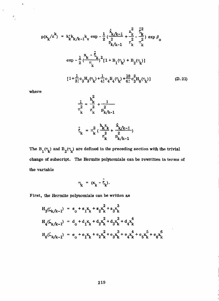
e
A
i xk/k-i
Pk/k-i
zk
+-_--_)rk _k
exp-_ TTk )2[i + Bl(_k ) + B2(_k)]
where
[i+'_.,OsHs('qk)+_c4H4<'qk)i02+_-.I c3H6(T _ ]
i h_ i- ÷
2 2 2
TTk rk Pk/k-i
(D. 2i)
A
_. )rk Pk/k-I
The Bl(_]k) and B2(r _ are defined in the preceding section with the trivial
change of subscript. The Hermite polynomials can be rewritten in terms of
the variable
First, the Hermite polynomials can be written as
H3(C,k/k 1) = s- O
H4(Ck/k_ 1) = do
H6(Ck/k 1) = e- O
2 3
+sixk +s2xk +SaXk
+ dlX k + d2x_+ d3x_+ d4x _
+elx k+e2x k+e 3 +e 4 +e5x k+e6x k
219

where
SO
^3
Df xk/k-__3_k/k-1_= -( 3 Pk/k-1
Pk/k-i
^2
Df _ 1
s 1 3( 3 Pk/k- 1Pk/k-1
A
s2 = -3 3'
Pk/k-1
Df 1
s3 = 3
Pk/k-1
and
do
^4 ^2
Df __6 _ +34 2
Pk/k-1 Pk/k-1
d 1
^3 ^
Df-4( 4 - 2
Pk/k-i Pk/k-i
^2
d2 = 6( - 2 ')
Pk/k-1 Pk/k-i
d3 --17_4-_4
Pk/k-1
Df 1d4 - 4
Pk/k-1
220
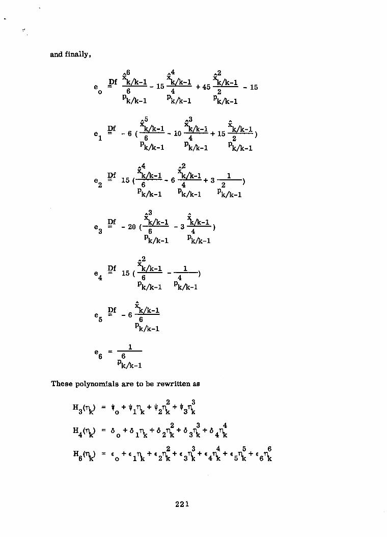
and finally,
eo
Df
^6 ^4 ^2
Xk/k-i - i5 Xk/k-i + 45 Xkfk-i6 4 2
Pk/k-I Pk/k-i Pk/k-i
- 15
eI
,,5
6
Pk/k-i
A3
_ 10 -_-:._ + 15 _/k-I )4 2
Pk/k-I Pk/k-i
^4 ^2
e 2 = 15( -6 +3 2 )
Pk/k-1 Pk/k-I Pk/k-i
e3
^3
Xk/k-i _ 3_--._)-20( 6 4Pk/k-i Pk/k-i
e4
Df
.,2
Xk/k-__41-_---)is( 6
Pk/k-i Pk/k-1
e 5
^
_Dr 6 _k/k-_6
Pk/k-i
1
e6 - 6
Pk/k-1
These polynomials are to be rewritten as
, 2H3(_k) = *o + *l_k + 2_k + *3_
H4(_k) = 5 +51_k+52r_+53_+54r_O
H6(_k) = co
2 3 4 5 6
221

The coefficients that satisfy the equality are found to be
_o_So÷_*__÷ s_^2
_1 = Sl ÷ 2S2_k ÷ 3s3_I_
_2 = s2 + 3S3_k
_3 = s3
50 0 k
51 = dl + 2d2_k + 3d3 + 4d4
52 = d2 + 3d3_k + 6d4_
^
= d 3 4d4_ k53 +
64
E0
E1
E2
E3 =
E4 =
5
d 4
e +el_ k+e 2 +e 3 + +e 5 +e 60
e_÷_e_÷ _o_÷ _e_÷_e_÷ 6o6_e_÷_e_÷6o_÷_Oe_÷_Oeo_o_+_e_÷_0o_÷_Oeo_e 4 + 5.5_ k + 15e6 _2
e 5 + 6e6_ k
E6 = e 6
222

c"
Let
Dfk --
0
^ 2 _2i Xk/k-1 Zk k
k_kvkk/k_ 1 exp - _ (2 + -2 - --2) exp _o
Pk/k-i rk Wk
1 1
0 O
1 (_k)211+ B12exp - 2 _k + B2]
1 10 -1+r., + +r.' l
Then,
k) 1p(xklz =+ 1 +I I0 2
E{[I+B l+B21[I _'!c3H3 _.vc4H4+_'!c3H6]]
i
O
1 (_k)2 [I+B 1"_exp - _ _k + B2I
1 1 +10 2[I+_Ic3H3+_.vc4H4 _.v c3H6]] (D. 22)
The moments E [_/z k] are computed in a straightforward manner. The
products of the polynomial terms appearing in (D. 22) are required. These
products are stated below for reference.
BIH 3 = So_l_ k + (So_21 + Slfll)_ + (So_31 + Sl/321+ S_l) _
6 7
+ (s?41 + s3f131)_ k + s3f141_ k
BIH 4 = dofll_ k + (doff21 + dlfll) _ + (doff31 + dlf121 + d2fll) _
4+ (doff41+ dlfl31+ d2_21 + dsfll)_k + (dlfl41+d2fl31+d3fl21+d4/_l)_
+ (d2f141+ d3f131+ d4f121)'r_+ (d3f141+ d4f131)_l_+ d4f141B_
223

B1H 6
B2H 3 =
B2H 4 =
_leo_k+ (_lel+fl21eo)_ + (_le2+_21el+fl31eo)r_
+¢1e3 + 2 e2 + 31el + 41eo) +¢1 4 + 2 e3 + 31e2
+ (_1e5 +f121e4 +f131e3 +f141e2)_ + (_le6 +f121e5 +f131e4 +fl4e3)r_
+ _821e6 +#31e5 +#41e4)_ + _31e6 +#4e5)_ + _41e6_ 0
s#22_ + (Slf122 + Sof132)_ + (Soft42 + Slfl32 +S 2_22 )lq4k
+ (So_5 + si_42 + S2f132+ s3f122)_ + (Soft6+Slfl5+ S2_42 + S3f132)+_
+ (Soft 7 +s i_6+ s2_ 5+ s3f142)_ + (Soft8 + Slfl7 + s2f16 + s3f15)_
ii+ (Sl_8+s2_ 7+ s3_6)_ + (s2fl8 + s3f17)_O + s3flSr _
do_22_+ (do_32 + dlf122)_ + (do_42 + dlf132+ d2f122)_
+ (d°_5 +dlf142+ d2f132+d3f122)_ + (do_6+ d1_5+ d2_42+d3f132+ d4f122)_
+ (do_7+dlfl6+d2f15+d3_42+ d4_32)_ + (do_8+ dlfl7+d2f16+d3f15+d4_42)_
+ (dlfl8+ d2f17 + d3f16 + d4fl5)r_+ + + 10(d2fl 8 d3fl 7 d4fl6)rlk
12+ (d3f18+ d4f17) r_l+ (d4f18) rtk
eof122_+ (e 1_22+ eo_32) r_+ (eo_42+ e 1_32+ e2_22) _
eft ,6+(e°_5+e1/_42+e2f132+e3f122)r_+(eo_6+el_5+e2_42+e3_32 + 4 22)_k
+ (eo_ 7+ e1_6+ e2_5+ e3_42+ e4f132+e5f122)r_
+ (eofl8+ e 1_7 +e 2fl6+ e3_5 +e4 _42 +e 5fl32 +e 6fl22)_
+ (elfl8+ e2f17+ e3f16+ e4f15+ e5f142 + e6f132 ) v_
10 11+ (e2f18+ e3f17+ e4_6+ esf15+ e6f142)rl k + (e3_8+ e4f17+ esf16 + e6_G)rl k
12 13 14+ (e4fl8+e5fl7+e6_6)rlk + (e5_8+e6fl7)Vlk +e6fl8rl k
%
224

After the moments E [r_/zk]t (l = 1, 2, 3,4) have been computed, the central
moments required for the Edgeworth expansion are computed from (D. 8)
through (D. 11) with the obvious change of subscript. This completes the
derivation.
225

e_RECI_D'II_G 1_8 BLANK NOT FIL_ED.
APPENDIX E
MOMENTS OF A DISTRIBUTION
The relation between the moments and the central moments are presented
in this appendix to provide a convenient reference. The central moments
through the twentieth are included.
5.1 MOMENTS OF A GENERAL DISTRIBUTION
Consider a random variable _ with finite moments of all order. The
central moments are related to the moments according to the following
schedule.
= a
E[(_ - a) 2] (y2
E[(_-a) 3] __Dr
E[(g - a) 4] =
E[(_-a) 5] __Dr
E[(_-a) 6] Df
E[(_ - a) 7]
E[_ 2] - a 2
U3
E[_ 3] - 3a 23
-a
%
E [_4] _ 4ala 3 _ 6a2o.2 _ a 4
U5
E[_5] _ 5ma4 _ 10a2 3 _ 10a3 2 _ a 5
= E[_ 6 ] - 6a_ 5 - 15a21.t4 - 20a31_3 - 15a 42 _ a 6
Df
E[_ 7 ] - 7al_ 6 - 21a2_5- 35a3bL4 - 35a41j3 - 21a 52 _ a 7
227

E[(_ - a)8] =Df
E[(_ - a)9]
%
= E[_8I - 8a_ 7 - 28a2_6 - 56a3_5 - 70a4_4
_56a5_3 - 28a6_ 2 _a 8
Df= _9
= E [_9] _ 9sP8 _ 36a2_7 _ 84a3_6 _ 126a4_5
- 126a5_4 - 84a6_3 -36aTff 2 a 9
E[(_ - a)II] =Dr
E[(_ - a)121 =Dr
E[(_ - a) 14] =Dr
_i0
E [_i0] _ 10a_ 9 _ 45a2_8 _ 120a3_7 _ 210a4_6
- 252a5_5 - 210a6_4 - 120a7_3 - 45aSff2 _ aI0
_11
E[_ 11] - lla_10 - 55a2_9 - 165a3_8 - 330a4_7 -462a5_6
- 462a6_5 - 330a7_4 - 165a8_5 - 55a9c 2 _ a ll
_12
E [_12] _ 12_lla _ 66_10 a2 _ 220_9a
- 792_7 a5 - 924_6 a6 - 792_5 a7
220_t3a9 66_2a10 12
3 4- 495_8a
8
- 495_4a
_113
E[g 13] - 13_12a- 78P.ll a2 - 286_10 a3 - 715_.9a4
- 1287_aga5 - 1716_a7a6 - 1716_6 a7 - 1287_t5a8
715_t4a9 286_3 al0 78_2 all 13
_14
E[_ 14] - 14_13a - 91_12 a2 - 364_11 a3 - 1001_t104
- 2002_9 a5- 3003_8a 6 - 3432_t7a7 - 3003_t6a8
- 2002_5 a9 - 1001_4 alO - 364_t3all - 91_2 a12
14-a
e
228

= _.5 2 455_12a3 - z365_zl 4= z[_zsl - 15_.l_a- xos_13a -
5_ 5oo5_.96 - 6435_.8aT- 6435_ as- 3003_tlOa 11 12
9 3003_t5#0 - 1365_4a - 455_3a.5005_.6a -
13 15
_ 105_2a - a
4
_16 2 _ 560_.z3a3 - is2o_12az[_161 z6_5a- _2o_14a s
- 7 12870_8a5 6 11440_9a -
- 4368_tlla - 8008_i0 a -I0 Ii . 1820_t4J2
9 _ 8008_6a - 4368_5a_ 11440_a
2 14 1613_1206 a -a
- 560_3a
4
E [_171 17_16 a - 136_tlSa " 680_t14a- "I 8
5 _ 12376_tll 6 - 19448_tlOa - 24310_9a_6188_tlZa 12
9 i0 _ 12376_6 a11 - 6188_5a
14 _ 136(_ a
_ 2380_4 a13 - 680_3a
a)_Sl D_Z [(_- =
4
_18 Z 3 3060_14 a
E [_18 ] _ 18_1_a - 153_16 a - 816_15a "6 '7
5
8 486g0_9 9 - 43"_58_8a- 43758_t10a - 13
12
1E 18 564_6a - 8 568_5a_ 318_4_a - 18
14 15. 153_a 16 -a
229

$
E[(_ - a)19] D_ _192 3 4
E[_ 19] - 19_19 a - 171_t17a - 969_16 a - 3876_15 a
5 6 7
_11628_14a - 27132_13a - 50388_t12a
8 9 10- 75582_11a - 92378_10 a - 92378_9a
11
- 75582_8a
14- 11628_5a
12 13
- 50388_7a - 27132_t6a
15 16
- 3876_4a - 969_3a
1712a 17 19-- -- a
E[(_ - a)2°] Df
=
_20
E [_20] _ 20_19a_ 190_18 a2 _ 1140_17 a3 - 4845_16 4
- I5504_15 aS- 38760_14 a6 - 77520_13 a7
8 9 10
- 125970_12 a - 167960_11 a - 184756_10 a
11 12 _ 77520_7 a13
15 16- 167960_9a - 125970_8a
14 _ 4845_4 a- 38760_6a - 15504_5a
17 _ 190a2a 18 _ a 20- 1140_a
E.2 MOMENTS OF A GAUSSIAN DISTRIBUTION
The central moments of a gausstan distribution have the properties that
_i = 0 , i=3,5,7,9, ....
_i --(i- i)_, i _ 4,6,s,...
Thus, the relations of the preceding section can be simplified for this distribu-
tion. These relations shall be stated explicitly below because they are of
considerable importance in the approximations presented elsewhere in this
document.
230

't
Let _ be a gaussian random variable with mean value a and variance (r 2.
s[_] =
s[_ 2] =
E[_ 3] =
E[_ 4] =
E[_ 5] =
E[_ 6] =
E[_ 7 ] =
E[g 8] =
E [_91 =
E[g I°] =
El{ II] =
E[_12] =
E[_ 13]
E [ _141
E[_ 16]
a
2 2O" +a
a(3ff 2 + a 2)
34 + 6a2(r 2 + a4
a(15 + 102a2+ 4)
5(76 + 454a 2 + 15a2a 4 + a 6
a(356 + 105o-4a2 + 812a 4 + a6)
7 8 + 1406a 2 + 2104a 4 + 280"2a 6 + a 8
a(63 8 + 4206a 2 + 3784a 4 + 362a 6 + a 8)
90 .10 + 3150-8a 2 + 10500.6a 4 + 6304a 6 + 45cr2a 8 + a 10
a(99(r 10 + l155q8a 2 + 23106a 4 + 9904a 6 + 55(r2a 8 + a 10)
11(y 12 + 594(rlOa 2 + 34658a 4 + 46206a 6 + 14854a 8
+ 66_2a 10 + a 12
a(1430 "12 + 25740"10a2 + 90098a 4 4-85800"6a 6 + 21450"4a 8
+ 780.2a 10 + a 12)
130 "14 + 10010"12a2 + 90090"10a4 + 210218a 6 + 150150 "6a8
+ 3003o-4a 10 + 912a 12 + a 14
a(195o "14 + 50050.12a2 + 270270.10a4 + 450450.8a 6
+ 25025O-6a 8 + 40950.4a 10 + 1050-2a 12 + a 14)
15o -16 + 1560o.14a2 + 200200r12a4 + 72072o.10a6
+ 900908a 8 + 400406a 10 + 54604a 12
+ 1202a 14 + a 16
231

a(255_16 + 88400.14a2+ 680680.124 + i75032(_10a6
+ i701700.8a 8 + 61880O-6a 10 + 7140a4a 12
+ 1360. 214 + a I6)
170 "18 + 22950.16a2 + 39780(714a4 + 204204(r12a6
+ 393822fflOa8 + 306306G8a 10 + 92820Cr6a 12
+ 91800.4a 14+ 1530.2a 16 + a 18
a(323Cr 18 + 145350.16a2 + 151164Cr14a4 + 554268(_12a6
+ 8314020.10a8 + 529074ffSa 10 + 135660(_6a 12
+ 116280.4a 14+ 171a2a 16 + a 18)
19or 20 + 3230Cr18a2 + 726750.16a4 + 503880(714a6
+ i3856700.12a8 + 1662804GlOalO + 881790_8a 12
+ 14535o.416 + 1900. 218 + a 20+ 193800G6a 14
e
232