AN ANALYSIS OF THE

DETERMINANTS OF FIJI’S IMPORTS

Annie Rogers

Working Paper

2000/03

May 2000

Economics Department

Reserve Bank of Fiji

Suva

Fiji

The author is grateful for helpful suggestions/comments from Mr.Steven Morling. The views expressed herein are those of the author andmay not necessarily reflect the views of the Reserve Bank of Fiji.

Abstract

In Fiji, imports as a share of GDP has been rising strongly,

particularly over the past three decades. Over these years imports have

fluctuated considerably, generally in line with fluctuations in aggregate

demand.

Fiji is a small island state, heavily dependent on external trade for

many of our essential goods. It is vital, therefore to always ensure that

we have adequate foreign reserves to pay for our import needs. It is

therefore important that we understand the factors determining import

demand and underpinning its growth and fluctuations. This will facilitate

balance of payments projections and allow for better forecasting of

foreign reserve levels.

In this paper, the behaviour of Fiji’s imports during the period

1968-1998 is studied and important factors that determine imports are

identified. The estimation of an error correction model enables the

separation of the short- and long-run elements of this relationship. The

study shows imports and domestic demand move contemporaneously in

the short-run in an almost one-for-one fashion. The real effective

exchange rate is also found to be a strong determinant of imports in the

short-term. In the long-run, domestic demand is the major determinant

of movements in imports in Fiji.

2

1.0 Introduction

One of the main objectives of monetary policy in Fiji is t o

maintain an adequate level of foreign reserves. To forecast the level of

foreign reserves requires substantive analysis of the components of the

balance of payments. Improvements in the balance of payments can

eventuate through changes in the current account or the capital account.

Within the trade component of the current account, a positive change is

determined by a reduction in imports or an expansion in exports. It is

therefore important for policymakers to identify the trends in both

elements of the trade account, in conjunction with other components of

the current account and the capital account, in order to better predict

the level of foreign reserves. This study endeavours to contribute to this

task by attempting to identify factors contributing to import growth. A

study carried out by Prasad (2000) analyses the determinants of exports

in Fiji.

Some understanding of import demand will also help formulate

policy on current and capital account liberalisation in Fiji. Knowing for

example, the extent to which changes in economic activity will likely

reduce or increase the amount of foreign currency flowing from the

country as import payments and having at hand a model which

facilitates the projection of these amounts is a useful tool to anticipate

balance of payments movements. It will also facilitate foreign reserves

forecasting.

Many overseas studies, including studies of developing countries,

find domestic activity/income and relative prices have a strong

correlation with imports, with many of these studies finding income t o

3

be the principal determinant of imports (Krugman, 1988; Horton and

Wilkinson, 1989; Wilkinson 1992; Catao and Falcetti, 1999; Reinhart,

1995; Senhadhi, 1998; Clarida, 1994; Goldstein and Khan, 1985; Yuan

and Kochhar, 1994).

To date, very little empirical research has been undertaken t o

identify the determinants of imports in Fiji. A paper by Joynson (1997)

provides some preliminary analysis. This paper found domestic demand

to be the dominant influence on imports in Fiji. Movements in the real

effective exchange rate were also found to play an important role.

The empirical model developed by this study will help explain

movements in imports and will also be useful for forecasting.

Unfortunately data on volumes of imported goods are not available,

constraining this study to an examination of the behaviour of the value

of imports. The study estimates the short- and long-run determinants of

Fiji’s imports by applying an error-correction approach to time series

analysis. Section two discusses the behaviour of imports in relation t o

economic activity, the real effective exchange rate, tariffs and oil

prices. Section 3 develops a conceptual framework for the analysis of

imports. In Section 4 the data required for estimation are described, and

the estimation procedure and diagnostics are discussed. Section 5

presents the results, both for the long- and short-run, and these results

and their implications are discussed in the final section.

4

2.0 Trends in Imports

It is not surprising to note that imports has been expanding in

Fiji, particularly in the past decade, given the country’s move towards

trade liberalisation. Trade liberalisation has continued in line with

agreements Fiji has entered into with organisations such as the World

Trade Organisation and has resulted in tariff rates being progressively

reduced.

Analysis of the import penetration ratio confirms Fiji’s outward

orientation. As shown in Figure 1 imports as a share of real GDP has

exhibited a trend rise, with the import penetration ratio now standing at

around 60 percent, compared with around 8 percent three decades ago.

FIGURE 1 Import Pen etration Ratio

05

1015

2025

30

354045

5055

6065

1968 1971 1974 1977 1980 1983 1986 1989 1992 1995 1998

%

Figure 2 shows imports expanded in most years over the past

three decades.1 Fiji’s imports mainly originate from Australia, followed

by the United States, New Zealand, Japan and the United Kingdom.

1 Data includes imports of aircraft.

5

These countries have consistently been the source of approximately 70-

75 percent of all imports over the past three decades.

FIGURE 2 Imports

(An nual perce nt ch ange)

-15- 10

- 50

510

1520

25

30

3540

4550

1969 1971197319751977197919811983 198519871989 1991199319951997

%

2.1 Domestic Activity

Theory on the marginal propensity to import suggests that a

certain proportion of an increase in income will be spent on purchases

of imports, suggesting that higher incomes should lead to higher

imports.2 If spending exceeds domestic supply, the shortfall will result in

higher imports. Therefore, the most important factor expected t o

influence the value of imports is the pace of domestic economic activity

and income changes.

2 All else equal, the higher are countries’ incomes per person the higher is trade (Frankel and Romer(1996); Frankel, Stein and Wei (1993)).

6

The relationship between economic activity and real imports is

shown in Figure 3, where the annual change in real gross domestic

product3 (GDP) is compared with imports.4 It is apparent that a strong

positive correlation exists between real GDP and imports. This

relationship was borne out by regression results of the study, which

showed real GDP and imports moving in an almost one-for-one fashion

in the short-run. The graph shows the pattern of growth in Fiji has been

very volatile5 over the study period and that changes in growth

generally move together with changes in imports. It is also evident that

the change in imports is more than proportional to that in GDP and this

appears to occur in most cycles of economic activity. Generally,

recessions have been accompanied by a fall in imports in the

corresponding and/or following year.6 A pickup in growth has generally

been accompanied by higher imports.

3 Real GNE was considered the appropriate activity variable as it represents domestic demand forgoods. However, due to the unavailability of real GNE data spanning the entire study period, realGDP was used instead. However the explanatory power afforded to activity is generally not alteredmuch by the choice of activity variable (Horton and Wilkinson (1989); Wilkinson (1992)).4 Unless otherwise specified, imports refer to the value of imports of goods and exclude “large items”such as aircraft. These items do not typically respond to changes in domestic demand.5 Williams and Morling (2000) describe more fully patterns of economic growth in Fiji over the sameperiod.6 Similar results were found in Dwyer and Kent (1993).

7

FIGURE 3 Real Imports and Economic Growth

(Annual percent change)

-25

-20

-15

-10

-5

0

5

10

15

20

25

1969 1973 1977 1981 1985 1989 1993 1997

%

Real Imports Economic Growth

Real imports = nominal imports/import prices

-

2.2 The Real Effective Exchange Rate

Fiji’s international trade performance is influenced, to some

extent, by the maintenance of a relatively stable real effective exchange

rate (REER). Its stability ensures that exporters can secure markets

abroad and achieve returns without undue exchange rate risk concerns.

Relative prices determine how much demand is spilled offshore.

8

FIGURE 4Real Imports and the Real Effective Exchange Rate

-25

-20

-15

-10

-5

0

5

10

15

20

25

1969 1973 1977 1981 1985 1989 1993 1997

%

0

20

40

60

80

100

120

140

160

Index

Real Imports(LHS)

REER(RHS)

Theoretically, movements in the REER are positively correlated

with the growth in real imports. This implies that an appreciation of the

REER will be a lower cost of imports, all other factors held constant.

This could lead to an increase in real imports demanded. Conversely a

fall or depreciation of the REER will be reflected in a higher cost for

imports leading to a decline in the volume demanded.

The graph above suggests movements in the REER for most

periods of the study have not particularly influenced imports. This was

likely due to the relative stability of the REER over this period.

However, in the devaluation years of 1987 and 1998 import volumes

declined quite substantially. This suggests that the weaker REER, which

has been translated into a higher cost of imports, has caused some

decline in imports in these years.

9

2.3 Tariff Reforms

The Fiji economy is more outwardly oriented today than it was a

decade or so ago, largely due to a trade liberalization policy that began

around 1988. Trade deregulation and tariff reforms were undertaken in

an attempt to align domestic and world prices.

Around this time over 50 percent of imports into Fiji were subject

to licensing requirements. In the August 1989 mini-Budget the

Government announced a major series of trade policy reforms. The

centrepiece of the reforms was the complete removal of import license

control on a large number of commodity imports. At the same time,

tariffs were adjusted on these items to provide alternative protection t o

local producers. Under this move, licenses on 31 categories of goods

were initially replaced with high tariffs of between 50-70 percent of the

value of imported goods.

In recent years Government has progressively reduced these high

tariff levels to bring down prices for consumers and as a continuing

signal for local industries to become competitive. In the 1991 budget the

standard fiscal tariff was reduced from 50 percent to 40 percent, and

then cut further to 30 percent in the 1992 budget. 1993 saw the general

tariff level reduced to 25 percent and then cut further to 22.5 percent in

the 1995 budget.

In the 1998 budget, however, tariff rates on items, which were

manufactured locally, were increased to a band at 35 percent. Also,

tariffs on most items that were not produced locally were reduced to a

standard rate of 10 percent. However, immediately after the January

1998 devaluation the government cut tariffs to reflect the change in

10

international competitiveness of domestic producers. In line with this

the duty on equivalent imported items manufactured locally was reduced

to 30 percent. The 1999 Budget outlined further tariff reductions. In

late August 1999, reductions in tariffs on some basic and essential food

items came into effect. Further reductions in fiscal duties were

foreshadowed in the 2000 Budget.

For 2000, Fiji’s tariff structure is divided into 3 bands for selected

industries and products. The tariff rates applicable in each band are 10

percent, 15 percent and 27 percent.

Despite the considerable erosion of tariff and non-tariff barriers

over recent years, growth in imports cannot automatically be attributed

to this factor although theoretically a rise in imports is expected as

tariffs fall. The relationship between real imports and average tariff

levels7 is shown in Figure 6. A negative correlation, as expected, was

generally observed suggesting a rise (fall) in tariff levels would result in

lower (higher) imports. Regression results from the study, however,

revealed only a weak negative correlation.8

7 Total duty paid on imports as a proportion of the total value of imports. Total duty comprises fiscalduty, customs duty and VAT. The introduction of VAT from 1st July 1992 led to the reduction in thelevel of import (fiscal) duties from 50% to 25%. Customs (and excise) duties have also been abolishedfrom this date other than on alcohol and tobacco products.8 Dwyer and Kent (1993) found the effective rate of assistance, used as a proxy for openness in theirstudy on Australia’s imports did not help explain the growth in aggregate imports, however it did proveto be a significant explanator of consumption and intermediate imports which account for the bulk ofAustralia’s total imports. It was found that a substantial share of the growth in these imports could beexplained by the reduction in protection.

11

FIGURE 5Real Imports and Average Tariffs

-25

-20

-15

-10

-5

0

5

10

15

20

25

1969 1973 1977 1981 1985 1989 1993 1997

%

0

5

10

15

20

Level

Real Imports(LHS)

Average Tariffs(RHS)

The apparent rise in average tariffs is due to the imposition of

VAT, from July 1993 that replaced higher fiscal duties that were earlier

levied, and is also likely to be influenced by better compliance and the

reduction of concessions.

2.4 Oil Prices

Over the past three decades oil prices have risen quite

substantially. However, as the graph below shows there has not been

much correlation between oil prices and imports. In the years of the oil

price shocks of 1974 and 1979/80 some decline in import volumes is

evident, however, other years in which oil prices fell, such as in 1986,

1991/92 and 1998, import volumes also declined.

12

FIGURE 6Real Imports and Oil Prices

-25

-20

-15

-10

-5

0

5

10

15

20

25

1969 1973 1977 1981 1985 1989 1993 1997

%

0

10

20

30

40Level

Real Imports(LHS)

Oil Prices(RHS)

3.0 The Conceptual Framework

Conventionally an import function is specified as a partial

adjustment model in which there is a time lag before the effect of

income changes is felt on import demand. The partial adjustment model

is basically a short-run model and neglects analysis of the very long-

term. Error correction models, on the other hand, isolate both the long-

and short-run behavioural responses while at the same time allowing for

lagged adjustment towards equilibrium by incorporating an error-

correction term. To allow for both long- and short-run analysis an

error-correction model was therefore used in this study. It is also

considered appropriate as full adjustment will likely not occur within a

short time frame due to costs involved in making short-run changes in

import volumes and as often trade contracts have already been entered

into.

13

A behavioural relationship can be specified to represent the

demand for imports, which in its simplest form could be a function of

domestic income. This study incorporates real GDP as an explanatory

variable and also takes into account changes in the real effective

exchange rate, and average tariff levels on imports.

The coefficient on the domestic activity variable shows the

response of imports to a change in income, or alternatively, the

marginal propensity to import, which measures the fraction of an extra

dollar of income earned that is spent on imports. This shows the extent

to which increases in disposable income will reflect in a deterioration in

the trade balance, via increases in imports, rather than in higher

domestic absorption.

A real effective exchange rate variable was also included in the

model. Movements in the REER affect resource allocation by changing

the country’s competitiveness in the international arena. A declining

REER effectively increases our competitiveness and supports our

exports but is reflected in higher import costs.

The import function was augmented with a term for average tariff

levels.

An increase in relative prices would be expected to lead to a

decline in the quantity of imports demanded. Both buoyant domestic

activity and a reduction in average tariffs would likely increase the

quantity of imports demanded.

The dependent variable, imports, depends upon importers’ desire

to purchase foreign goods as well as a shortfall in domestic supply. The

equilibrium quantity of imports is the product of interaction between

demand and supply in the market for importables. Demand can be

14

satisfied from two sources: the foreign supply of imports or the

domestic supply of substitutes.

However the determinants of supply are more complex than

those of demand (Leamer and Stern (1970)). A small country

assumption was invoked whereby an infinite elasticity of supply is

assumed so that the equilibrium quantity of imports can be related solely

to changes in demand (Murray and Ginman (1976)).

An import price deflator is not available for Fiji. A proxy was

constructed (see Appendix) to control for the effects of import prices

on nominal import values. While the import deflator would normally be

constrained to 1 in an import equation, there is a risk that if the proxy

measure is a weak indicator of import prices, the other coefficients in

the equation would be biased by the imposition of the unit constraint.

Accordingly, the price term was unconstrained in the estimation. The

estimated coefficient was significantly different from 1, confirming that

the constraint would have been inappropriate. A caveat to the results,

therefore, is that the price effects are only weakly controlled in the

equation.

15

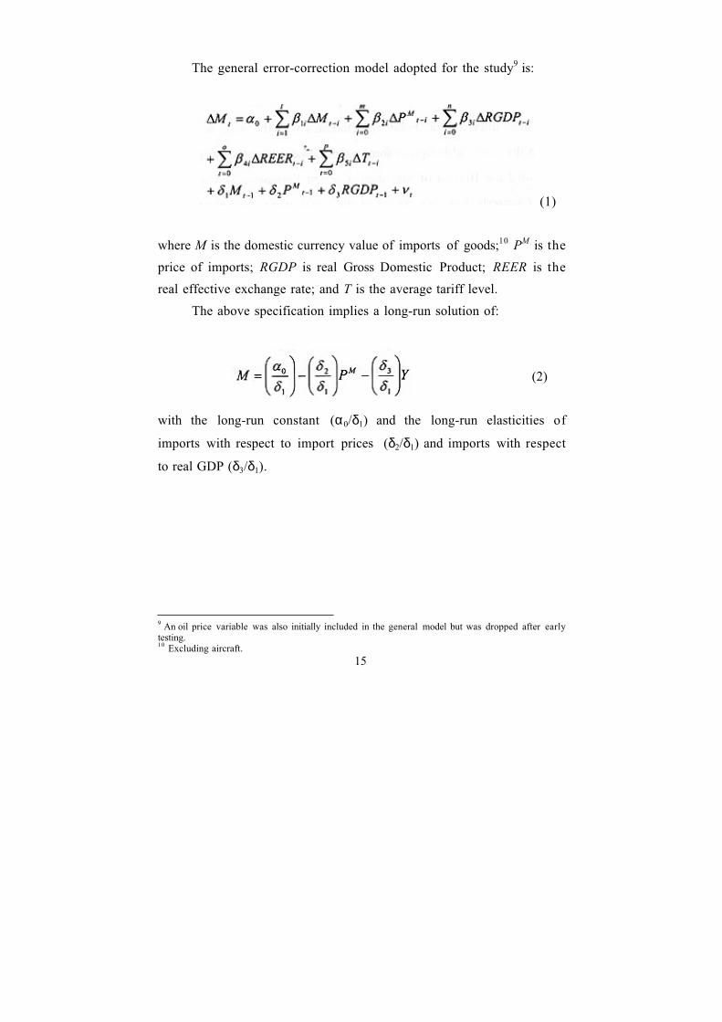
The general error-correction model adopted for the study9 is:

(1)

where M is the domestic currency value of imports of goods;10 PM is the

price of imports; RGDP is real Gross Domestic Product; REER is the

real effective exchange rate; and T is the average tariff level.

The above specification implies a long-run solution of:

(2)

with the long-run constant (α0/δ1) and the long-run elasticities of

imports with respect to import prices (δ2/δ1) and imports with respect

to real GDP (δ3/δ1).

9 An oil price variable was also initially included in the general model but was dropped after earlytesting.10 Excluding aircraft.

16

4.0 Empirical Results

4.1 Data

The IMF International Financial Statistics was the main source of

data used in the study, although in some cases domestic sources were

used. These included the Bureau of Statistics’ Current Economic

Statistics and the RBF’s Quarterly Reviews. Some of the series were

constructed from primary data. The Appendix provides a description of

data sources and details methods of construction.

Valid estimation of the model requires an examination of the

time-series properties of the data. Firstly all time series used in the

estimation process were tested for stationarity. Table 1 shows the results

of the standard Augmented Dickey-Fuller (ADF) (Said and Dickey 1984)

and the Phillips and Perron (1988) tests where a unit root null

hypothesis is tested against a stationary alternative.

Empirically, (the logs of) imports, import prices, domestic

output, the real effective exchange rate, tariffs and oil prices were found

to be integrated of order 1.

17

Table 1: Unit Root Tests

Estimation period: 1968 - 1998

Variable Dickey – Fuller Test Phillips – Perron Test

I(1) I(2) I(1) I(2)

Value of Imports -2.378 -2.835 -2.526 -4.745**

Import prices -1.337 -4.434** -1.465 - 3.243*

Gross DomesticProduct

-3.066* -3.524* -2.775 - 6.189**

Real effectiveexchange rate

-0.487 -3.054* -0.481 -2.677

Tariffs

Oil Prices

-1.370

-2.598

-3.015*

-3.509*

-1.474

-2.330

-4.904*

-5.870**

Notes: **(*) denotes significance at the one (five) per cent levels. The criticalvalues for the Augmented Dickey – Fuller tests I(1) are –3.675 and –2.967 atthe one and five percent levels respectively. The critical values for the Phillips– Perron tests are –3.666 and –2.963 at the one and five percent levelsrespectively.

4.2 Estimation

The model, specified in equation 1, is estimated as an unrestricted

error correction model (ECM) over the period 1968 to 1998. This

approach is recommended over the two-step Engle-Granger procedure,

which provides an alternative way to separate the long-and short-run

properties of the relationship.

This specification has an added advantage in that it isolates the

speed of the adjustment parameter, δ1, which indicates how quickly the

system returns to equilibrium following a random shock. The error

correction coefficient also tests for cointegration. When variables are

cointegrated, it implies that there is some adjustment process that

returns variables to their long-run relationship following a shock. A

18

general unrestricted ECM was estimated and the results are presented in

Table 3. In order to improve the accuracy of the significant coefficient

estimates, those variables whose coefficients were statistically

insignificant were excluded from the model.

4.3 Diagnostics

Before analysing the results, statistical properties of the model

were first assessed. Diagnostic tests were carried out to test for

normality, serial correlation, autoregressive conditional

heteroskedasticity, heteroskedasticity, specification error and stability.

The results of these diagnostic tests are reported in Table 2, and suggest

that the model is reasonably well specified. These results showed the

residuals are normally distributed, homoskedastic and serially

uncorrelated and the parameters appear to be stable.

19

Table 2: Diagnostics

Probability

Normality:

Jarque-Bera statistic χ2-statistic 0.877 0.645

Serial Correlation:

Breusch-Godfrey Serial F-statistic 4.136 0.321

Correlation LM Test χ2-statistic 8.778 0.246

AR Cond. Heteroskedasticity

ARCH LM Test F-statistic 0.165 0.688

χ2-statistic 0.176 0.675

Heteroskedasticity:

White Heteroskedasticity Test F-statistic

χ2-statistic

0.461

9.029

0.922

0.829

Stability:

Chow Breakpoint Test(mid sample)

F-statisticsL-R statistic

0.925 12.730

0.5250.121

Chow Forecast Test(1990-1998)

F-statisticsL-R statistic

1.297 14.839

0.3960.001

Specification Error:

Ramsey RESET Test F-statistics

L-R statistic

0.812

2.342

0.458

0.310

Notes: **(*) denotes significance at the one (five) per cent levels. No terms weresignificant at these levels. LR is a likelihood ratio statistic.

5.0 Results

The results presented in Table 3 suggest that domestic activity

and the real effective exchange rate have an important role to play in

influencing imports in Fiji. The explanatory power of the ECM model is

20

relatively high at around 75 percent. The results show that the value of

imports depend positively on the level of GDP and the real effective

exchange rate and negatively, to a small extent, on tariffs. Also, the

study found that the long-run output elasticity of imports is considerably

higher, almost double, than that in the short run.

Figure 7 shows that the model fits the data quite well. The

equation’s standard error is 0.06 percent, indicating that about two

thirds of the time, the predicted value is within about 6 percentage

points of the actual value.

This suggests that there is still a substantial margin of error and

has important implications for any forecasting of imports which may be

undertaken and which may underpin policy decisions. The model,

however, can reasonably be used for predictive purposes and in

forecasting expected values of imports.

Long run

The long-run coefficient for real GDP suggests a roughly two-fold

increase in the value of imports in line with increases in output.11 The

results suggest that increased growth will likely result in a substantial

increase in imports in the long run. This shows that income increases

are likely to be reflected in higher consumption and given the limited

range of consumption and investment goods produced domestically, the

stronger demand is likely to translate into higher imports.12

11 The value of the coefficient may be understated because of the less than unit coefficient on theunrestricted price term.

21

Table 3: Determinants of Imports (Unrestricted ECM)

Dependent variable: growth in imports; estimation period 1968 - 1998

Explanatory variables: short run (1) (2)

Constant -6.6425(-2.618)*

∆ Import pricest 0.5291(2.462)*

∆ Real Gross Domestic Productt 0.9031 (2.941)**

∆ Real Effective Exchange Ratet 0.7579 (2.831)**

∆ Tariffst -0.0178 (-1.943)

Explanatory variables: long run

Imports value t-1 -0.7331 (-3.757)**

Real Gross Domestic Product t-1 1.2908

(2.691)**

1.7608 (5.973)**

Import prices t-1 0.4120

(3.800)**

0.5621

(4.655)**

Summary statistics

Adjusted R2 0.749

σ 0.062

Notes: t-values are in parentheses. **(*) denotes significance at the one (five) percent levels. For the long-run explanatory variables, the implied long-runcoefficients (column 2) were calculated as the ratio of the relevant long-runECM coefficients to the long-run coefficient on the lagged dependentvariable; the Bewley transformation was applied to obtain interpretable t-statistics. The cointegration test proposed by Kremers, Ericsson and Dolado(1992) is employed. σ is the standard error of the equation.

12 Reinhart (1995) found an income elasticity of industrial countries’ demand for imports of 2.5,compared with an elasticity of 1.22 for developing countries. See also Clarida (1994) and Marquez(1989).

22

FIGURE 7 Actual and Predicted Imports (Value) Growth

-0.18

-0.12

-0.06

0.00

0.06

0.12

0.18

0.24

0.30

0.36

0.42

1969 1973 1977 1981 1985 1989 1993 1997

Log Diff

Actual

Fitted

Short-run

The most prominent factor determining imports in the short-run

appears to be domestic income. The coefficient on the real GDP term is

close to one indicating that in the short run imports have grown close t o

one-for-one with output growth in the Fiji economy. A one percent

increase in GDP would cause imports, after controlling for prices, t o

increase by around 0.9 percent, confirming the pace of domestic demand

as a very important factor. This is in line with various studies, which

have shown domestic activity to be the principal determinant of

imports in other countries.

The next most important factor determining imports was the

REER. A one percent increase in the REER causes imports to rise by

around 0.8 percent. Given that an increase in the REER effectively

reduces the cost of imports, this result implies a rise in volumes

imported.13

13 See Cerra and Dayal-Gulati (1999). Reinhart (1995) found relative prices were importantdeterminants of imports in 11 out of 12 countries studied.

23

A small negative correlation between imports and average tariff

levels was evident with a one percent fall in average tariffs resulting in

only a marginal increase in imports. This suggests that lower average

tariffs, as measured in the study, only very marginally explains the

growth in imports in Fiji.14 However as imports are not a homogenous

bundle of goods, aggregating imports, as done in this study, may mask

important differences in the effect of falling tariff levels on the market

for different categories of imports.15

Other quantitative restrictions were tested within the scope of

the model, but were removed following tests, which showed a lack of

significance.

6.0 Conclusions

This paper has estimated an import function for Fiji on the basis

of cointegration analysis and an error correction model. It incorporates

real GDP, import prices and real effective exchange rate variables, as

well as a measure for average tariffs. Use of the error-correction

methodology allowed the long- and the short-run elements of the

relationship between the variables to be determined.

The results of the study show movements in domestic demand and

the real effective exchange rate predominantly explain movements in

imports.

The results emphasised the strong effect domestic activity has on

imports. It also showed that a higher cost of imported goods due to a

14 An earlier study, Joynson (1997), included foreign exchange reserves and the provision ofdomestic credit variables but found they are not constraining factors on the value of imports in Fiji.15 See Dwyer and Kent (1993).

24

depreciation of the REER will likely lead to a decline in the value of

goods imported. With an exchange rate depreciation, imports would

become relatively more expensive and would likely lead to lower

volumes imported.

Fiji’s economy is heavily dependent on a few major sectors such

as sugar, garments and tourism. Fluctuations in production and earnings

in these sectors lead to fluctuations in overall output of the economy

and result in swings in imports and our balance of payments position.

Monetary and fiscal policies, therefore, are needed to moderate swings

in output and to help achieve a steady and sustainable growth in real

GDP. This will also help moderate swings in imports and our foreign

reserves.

In the long-term the key risk to the balance of payments is Fiji’s

dependence on a few commodities to support its export earnings. Limited

production capacity and rising import demand, places pressure on the

balance of payments. A possible downturn in the sugar industry and any

weakness in the garment industry in the future would weaken the export

earnings base of the economy. It is important, therefore for production to

be diversified, in order to weaken this strong reliance on only a few major

export industries and to decrease imports. Strategic plans also need to be

put in place to increase productivity and international competitiveness in

our export industries so that the export sectors of the economy can face

competition as preferential access, under which most of our major exports

are traded, is eroded or expires. A freeing up of the economy should also

25

be undertaken so that resources may be employed where there is excess

demand.

More effective policy, therefore, should concentrate on

expanding our export-base and limiting the inflow of imports through

the development of “efficient” domestic producers where a comparative

advantage exists.

26

Appendix

Data Sources and Construction

Series Sources and Construction

Imports Import values of goods, exclusive of aircraft (fob).

IMF International Financial Statistics Yearbook (1998);Budget 2000;Bureau of Statistics.

Import prices Calculated as an index of export unit values of Fiji’s five major tradingpartners (in $US), weighted by their respective import share, converted intodomestic currency at period average official exchange rates.

IMF International Financial Statistics Yearbook (1998);IMF International Financial Statistics, various issues;IMF, Direction of Trade Statistics, various issues.

GrossDomesticProduct

Gross domestic product at constant factor cost.

IMF International Financial Statistics Yearbook (1998);Bureau of Statistics, Current Economic Statistics, various issues;Reserve Bank of Fiji, Quarterly Review (1999).

Real effectiveexchange rate

AverageTariffs

Real effective exchange rate as calculated by the Reserve Bank of Fiji. Forthe period prior to 1979 an index was constructed using the trade-weightedconsumer prices indices and bilateral exchange rates of Fiji’s five majortrading partners.

IMF International Financial Statistics Yearbook (1998);IMF International Financial Statistics, various issues;Reserve Bank of Fiji, Quarterly Review (1999).

Total duty paid on imports as a proportion of the total value of imports. Totalduty comprises fiscal duty, customs duty and Value Added Tax.

Ministry of Finance and Ministry of National Planning, Budget Address;Supplement to the Budget Address, various issues;Bureau of Statistics, Current Economic Statistics, various issues.

27

References

Banerjee, A., J. Dolado, J.W. Galbraith and D.H. Hendry (1993). Co-

integration, Error-Correction, and the Econometric Analysis of

Non-Stationary Data, Oxford University Press, Oxford.

Bewley, R.A. (1979). The Direct Estimation of the Equilibrium

Response in a Linear Dynamic Model, Economic Letters, 3, pp.

357-361.

Catao, L. and E. Falcetti (1999). Determinants of Argentina’s External

Trade, IMF Staff Paper, 99/121.

Cerra, V. and A. Dayal-Gulati (1999). China’s Trade Flows: Changing

Price Sensitivities and the Reform Process, IMF Working Paper

99/1.

Clarida, R.H. (1994). Co-integration, Aggregate Consumption, and the

Demand for Imports: A Structural Econometric Investigation,

American Economic Review, 84, pp. 298-308.

Dwyer, J. and C. Kent (1993). A Re-examination of the Determinants

of Australia’s Imports, Reserve Bank of Australia Research

Discussion Paper 9312.

Frankel, J., E. Stein and S. Wei (1993). Trading Blocs and the

Americas: The Natural and the Unnatural, and the Super-natural,

Journal of Development Economics, 47, pp. 61-95.

28

Frankel, J. and D. Romer (1996). Trade and Growth: An Empirical

Investigation, National Bureau of Economic Research Working

Paper 5476.

Goldstein, M. and M.S. Khan (1985). Income and Price Effects in

Foreign Trade, Handbook of International Economics, 2, pp.

1041-105.

Horton, T. and J. Wilkinson (1989). An Analysis of the Determinants

of Imports, Reserve Bank of Australia Research Discussion Paper

8910.

Joynson, N. (1997). Determinants of Import Values, Reserve Bank of

Fiji, Working Paper, unpublished.

Kremers, J.J.M., N.R. Ericsson and J.J. Dolado (1992). The Power of

Cointegration Tests, Oxford Bulletin of Economics and Statistics,

54(3), pp. 325-348.

Krugman, P. (1988). Differences in Income Elasticities and Trends in

Real Exchange Rates, National Bureau of Economic Research

Working Paper 2761.

Leamer, E.E. and R.M. Stern (1970). Quantitative International

Economics, Allyn and Bacon, Boston, pp.2-40.

29

MacKinnon, J.G. (1991). Critical Values for Cointegration Tests in R.F.

Engle and C.W.J. Granger (eds.), Modeling Long-Run Economic

Relationships, Oxford University Press.

Marquez, J. (1989). Income and Price Elasticities of Foreign Trade

Flows: Econometric Estimation and Analysis of the U.S. Trade

Deficit in L.R. Klein and J. Marquez (eds.), Economics in Theory

and Practice: An Eclectic Approach, Kluwer Academic Publishers,

the Netherlands, pp.126-76.

Mazarei, A. (1995). Imports Under a Foreign Exchange Constraint: The

Case of the Islamic Republic of Iran, IMF Working Paper 95/97.

Murray, T. and P.J. Ginman (1976). An Empirical Examination of the

Traditional Aggregate Import Demand Model, The Review of

Economics and Statistics, LVIII(I) pp. 75-80.

Perron, P. (1988). Trends and Random Walks in Macroeconomic Time

Series: Further Evidence from a New Approach, Journal of

Economic Dynamics and Control, 12(2/3).

Phillips, P. and P. Perron (1988). Testing for a Unit Root in Time

Series Regression, Biometrika, 75, pp. 335-346.

Prasad, S. (2000). Determinants of Exports in Fiji, Reserve Bank of Fiji,

Working Paper, underway.

Reinhart, C.M. (1995). Devaluation, Relative Prices and International

Trade, IMF Staff Papers, 42(2), pp. 290-312.

30

Said, S.E. and D.A. Dickey (1984). Testing for Unit Roots in

Autoregressive Moving Average Models of Unknown Order,

Biometrika, 71, pp. 599-607.

Senhadhi, A. (1998). Time-Series Estimation of Structural Import

Demand Equations, IMF Staff Papers, 45(2), pp. 236-268.

Wilkinson, J. (1992). Explaining Australia’s Imports: 1974-1989,

Economic Record, 68(201), pp.151-164.

Williams, G. and S. Morling (2000). Modelling Output Fluctuations in

Fiji, Reserve Bank of Fiji, Working Paper 00/01.

World Bank (1990). Fiji: Challenges for Development, Report No 7724-

Fiji, pp. 18-34.

Yuan, M. and K. Kochar (1994). China’s Imports: An Empirical

Analysis Using Johansen’s Cointegration Approach, IMF Working

Paper 94/145.