a dynamic analysis of france’s external trade determinants … · determinants of merchandise...

A DYNAMIC ANALYSIS OF FRANCE’s EXTERNAL TRADE

Determinants of Merchandise Imports and Exports

and their Role in the Trade Surplus of the 1990s

by

Tassos Belessiotis and Giuseppe Carone (*)

(*) The authors are, respectively, economist at the National Economies Directorate, DG-II A-3, EC

Commission, Brussels, and research economist, Istituto Nazionale per lo Studio della Congiuntura(ISCO), Roma. We wish to thank Nathalie Darnaut who read various drafts of the paper andprepared the material for section II.a, and especially Antonio Cabral for supporting the project andfor many very helpful comments which clarified the argument. The paper, responsibility for whichremains ours, reflects the authors’ opinions and not the Commission’s or ISCO’s.

A DYNAMIC ANALYSIS OF FRANCE’s EXTERNAL TRADE

Determinants of Merchandise Imports and Exports

and their Role in the Trade Surplus of the 1990s

I. Introduction........................................................................................................................1II. Some salient features of France’s external performance in recent years .........................4II. a 7UDGH�SDWWHUQV��4II. b 'HYHORSPHQWV�LQ�SULFH�DQG�FRVW�FRPSHWLWLYHQHVV��6II. c ,PSRUW�SHQHWUDWLRQ��H[SRUW�LPSRUW�UDWLRV��DQG�H[SRUW�PDUNHW�VKDUHV ��10II. d 'HPDQG�GHYHORSPHQWV�LQ�)UDQFH�DQG�DEURDG..............................................................13III. Factors underlying the trade surplus of the 1990s ..........................................................15IV. Econometric methodology and modelling strategy..........................................................17,9��D 6SHFLILFDWLRQ�RI�WUDGH�IXQFWLRQV .....................................................................................17,9��E (FRQRPHWULF�PHWKRGRORJ\ ............................................................................................19,9��E�� 8QLW�URRW�DQDO\VLV ..........................................................................................................20,9��E�� &RLQWHJUDWLRQ�DQDO\VLV��21V. Determinants of imports: Specification and estimation results.......................................24VI. Hysteresis in imports and stability of the estimates.........................................................30VII. Determinants of exports: Specification and estimation results.......................................34VIII. Hysteresis in exports and stability of the estimates.........................................................39IX. France’s external constraint and economic growth .........................................................41X. The trade surplus of the 1990s: Evidence from simulations ..........................................44XI. Concluding remarks ........................................................................................................46

Annex A: Sources and time-series properties of the data...............................................................48Annex B: Further cointegration results, import equations ...............................................................50Annex C: Stability of dynamic import equations ..............................................................................53Annex D: Stability of coefficients of dynamic import equations.......................................................54Annex E: Further cointegration results, export equations ...............................................................57Annex F: Stability of cointegration vectors, export equations .........................................................59Annex G: Stability of dynamic export equations ..............................................................................60Annex H: Stability of coefficients of dynamic export equations.......................................................61

References .........................................................................................................................................64

A DYNAMIC ANALYSIS OF FRANCE’s EXTERNAL TRADEDeterminants of Merchandise Imports and Exportsand their Role in the Trade Surplus of the 1990s

,��,QWURGXFWLRQ

One of the striking characteristics of France’s economic performance since the beginning ofthe present decade has been the strength of the external accounts. In particular, on the basisof national accounts data, since 1989 the current account and the non-energy trade balancehave recorded rising surpluses, which in 1996 amounted to 1.7 % of GDP and to close to 1.5% of GDP, respectively. The service balance, on the other hand, has registered persistentsurpluses which averaged between 1 and 1.4 percent of GDP in the 1990s. The largestcomponent of merchandise trade is trade in manufactured goods1. The balance onmanufacturing trade recorded surpluses throughout the period following the 1973 oil crisis tothe late 1980s. The manufacturing trade balance slipped into deficit in the period 1987-1991but subsequently moved into surplus which rose to almost 1 % of GDP in 1996. Graph 1presents quarterly data on the evolution of these variables from the beginning of the 1970s tothe end of 1996; data adjusted for inflation present a similar picture. It is clear that sincemovements in the current account are dominated by movements in the non-energy and, inparticular, in the manufacturing trade balance throughout this period the sources of thecurrent account improvement in the 1990s are likely to be those explaining the improvementof the manufacturing trade balance.

Awareness of the importance of developments in France’s external transactions became morepronounced following the commitment to sustain a stable franc in the ERM. Externalaccounts deficits were considered as leading to devaluations and, consequently, exchangerate stability required that the trade balance was not systematically in deficit, in order not toundermine exchange and the stability2. Since the dominant component of France’s externaltransactions is trade in manufactures, the commitment to a stable franc inevitably implied thenecessity to strengthen the manufacturing trade balance, principally through improvements incompetitiveness. These took the form of cost and price restraint which has had a beneficialeffect on export growth and on the manufacturing trade balance, and on supporting theexternal value of the franc3.

Graph 1 also shows the importance of manufacturing in France’s external and, morespecifically, in non-energy trade. Over much of the period since the beginning of the 1970speaks and troughs in the former coincide with peaks and troughs in the latter, while the level

1 Developments in the overall merchandise trade balance over the period since the early 1970s to 1987 have

been the result of persistent deficits in energy trade largely offsetting surpluses in trade in manufacturesand in agricultural and food products. Since 1985 the deficit in energy trade has been diminishing and by1994 it was back to its value of the early 1970s of around F 75 billion (FOB-CIF basis). The principalcontributor to the merchandise trade deficits of the period 1987-1992 was the deficit in trade inmanufactures.

2 See Bonnaz et Paquier (1993).3 The policy of strengthening competitiveness through price and cost restraint rather than through nominal

exchange depreciation is associated with the notion of competitive disinflation; Muet (1992) andBlanchard and Muet (1992) discuss these issues in detail.

- 2 -

of the manufacturing trade balance accounts on average for virtually the level of the non-energy trade balance. This relationship has been particularly close in the period up to thesecond half of the 1980s. Since then, a systematic deviation has emerged where the level ofthe manufacturing trade balance has been lower than the level of the non-energy tradebalance. Furthermore, since 1987 improvements in the non-energy trade balance have beenlarger than those in trade in manufactures where notably larger deficits have been recordeduntil late 1991. Clearly, marked improvements in non-manufacturing, non-energy trade (thatis, trade in agricultural and food commodities) are at the background of these developments.By 1996, the non-energy trade balance had registered surpluses amounting to over 1 percentof GDP while the manufacturing trade balance had recovered from a peak deficit of 0.7percent of GDP recorded at the end of the 1980s and in the beginning of the 1990s to asurplus of 0.7 percent of GDP in the first three quarters of 1996. This improvement hastaken place against a background of turbulence in the ERM marked by the substantialnominal and real depreciations of the exchange rate for the Italian lira, the Spanish peseta,the Portuguese escudo, and the British and the Irish pound against the French franc4.

4 The bilateral nominal French franc exchange rate for the lira and the peseta peaked at 37.9% and 26.2%,

respectively, in April 1995 relative to January 1990; the exchange rate for the escudo peaked at 14.9% inDecember 1995; and the exchange rate for the Irish pound and for sterling peaked at 12.7% and 19.7%,respectively, in November 1995. The Swedish krona was not part of the ERM in the early 1990s when italso experienced substantial depreciations against the ERM currencies. Between January 1990 andSeptember 1992 the krona exchange rate in the European currencies was stable, but from September 1992to December 1993 the krona/French franc nominal exchange rate had appreciated by 31.4%, and therewas another sharp appreciation in April 1995 when relative to September 1992 it had appreciated by39.4%. Some of this has now unwound but the krona remains around 22% of its French franc value inSeptember 1992. Bilateral real exchange rates, more on which is discussed in section II.b below, showsimilar behaviour.

Graph 1Non-energy, manufacturing, and current account balance

(percent of GDP)

-2

-1

0

1

2

3

70 72 74 76 78 80 82 84 86 88 90 92 94 96

Manufactures Non-energy Current account

Source: Commission services

- 3 -

There are three significant factors which have undoubtedly contributed to France’s externalperformance in recent years. First, the different cyclical position of France relative to itsmain trading partners; secondly, relative price developments which have moved to France’sadvantage or disadvantage principally, but not exclusively, as a result of nominal and realexchange rate changes; and, third, supply improvements which have promoted exportexpansion and import substitution, principally through gains in cost and pricecompetitiveness but also through improvements in non-price competitiveness associated withchanging technology through new investment5 in the trading sectors of the economy,increased export capacity, productivity-induced relative price changes etc. The impact of thefirst two factors has likely dominated, especially in short-term developments, the latter’sinfluence on France’s trade. Ultimately, however, many supply-side improvements haveundoubtedly themselves taken the form of improvements in France’s relative costs andrelative prices.

The purpose of the present paper is to review the sources of France’s trade surplus in recentyears and to attribute trade balance movements strictly to those determinants of trade flowssuggested by economic theory. These determinants are price and/or cost developments, anddemand in France and in the rest of the world. Nominal exchange rate movements in the1990s have been perceived as playing a significant role in France’s trade performance,particularly during the depreciation episodes of 1992 and 1993, since they were considered tohave imparted a competitive advantage to those trading partners whose currency haddepreciated against the franc; ceteris paribus, and assuming that the nominal depreciationled to a real exchange depreciation, imports would increase and exports would decline, andthe trade surplus in real terms would decline. This could have permanent effects on the tradebalance since, according to some models of international trade, prolonged exchange rateappreciations, or depreciations can induce hysteresis phenomena (see Baldwin (1988), forexample). At the same time, slow growth in France relative to the rest of the world in the1990s would be expected to have led to a widening of the trade surplus. These two factorshave a conflicting impact on trade balance movements, and since income elasticities aregenerally substantially larger than relative price elasticities it is possible to argue that theemergence of the trade surplus since the beginning of the 1990s is dominated by relativedemand movements. A primary objective of the paper is to examine the empirical supportfor these propositions and to analyse the dynamics of adjustment of trade flows to changes incompetitiveness and in relative demand. To do so, a cointegration/error-correction model isapplied to flows of both imports and exports, and the estimates of key elasticities obtainedare instrumental in shedding light on this question.

The paper, in addition to the introduction, is organized as follows: Section II reviews somesalient characteristics of France’s trade in recent years in terms of trade patterns, price andcost competitiveness developments, import penetration and export market performance, andin terms of demand developments in France and abroad; section III discusses an accountingdecomposition of movements in the non-energy and in the manufacturing trade balance overthe period 1990 to 1996 according to the state of price competitiveness and of relativedemand; section IV presents the econometric methodology used in the empirical work;section V examines the error-correction model for non-energy and manufacturing imports;

5 Francq et Lamoit (1990) attribute the better export performance of Germany compared to France to

Germany’s investment dynamism. More investment in the internationally trading sector of the economymakes possible, among other things, greater than otherwise response to demand shocks. Investment inGermany’s manufacturing sector during the post-1985 recovery of world trade notably exceeded thecorresponding investment in France - see Francq et Lamoit (1990).

- 4 -

section VI examines the possibility of hysteresis in imports through equation stability tests;section VII examines the corresponding model for non-energy and manufacturing exportsand section VIII reviews the question of hysteresis in exports again through equation stabilitytests; section IX uses elasticity estimates from the econometric estimation to shed light onthe relationship between the trade balance and demand and competitiveness developments;section X presents simulation results for the non-energy and the manufacturing trade balancesince the beginning of the 1990s where the contribution of price competitiveness and ofrelative demand is evaluated; and, finally, section XI presents conclusions.

There are eight annexes complementing the paper. The sources and the time seriesproperties of the data are presented in Annex A; Annexes B, C and D present additionalcointegration results and further evidence on the stability of the import equations; andAnnexes E, F, G, and H are devoted to reviewing further cointegration results and toexamining the stability of the export functions.

,,��6RPH�VDOLHQW�IHDWXUHV�RI�)UDQFH¶V�H[WHUQDO�SHUIRUPDQFH�LQ�UHFHQW�\HDUV

,,��D 7UDGH�SDWWHUQV

Most of France’s international trade is conducted with other European and, more specifically,European Union States, reflecting the progressive liberalization of the past thirty or so yearsundertaken in the context of European integration. According to customs data (which are notimmediately comparable to the national accounts data shown in Graph 1 and usedsubsequently in the empirical work), the average share of intra-EU merchandise exports inthe decade of the 1970s was 56.6%; as can be seen in Table 1, this share declined marginallyin the 1980s, but advanced to 61.3% in the first half of the 1990s. Intra-EU exports of

manufacturedgoods advancedeven moremarkedly betweenthe 1970s and the1990s, rising bysome 6.2percentage pointsof the total to58.6%. Theorigin ofmerchandiseimports, on theother hand, hasshown morediverse patterns.The share of intra-EU imports rosefrom 54.3% of

total merchandise imports in the 1970s to 63.9% in the first half of the 1990s, an increase ofalmost ten percentage points in twenty five years. However, opportunities to widen thesources of imports have also expanded during this period. Imports of manufactures, the mosthighly income-elastic component of merchandise imports, have increasingly been sourced

Table 1The composition of non-energy trade and of trade in manufactures

(annual averages as percent of total; balances in Ecu million, customs data)

Intra-EU Extra-EU

1970-79 1980-89 1990-94 1970-79 1980-89 1990-94

Merchandise exports 56.6 55.9 61.3 43.4 44.1 38.7

RI�ZKLFK��1RQ�HQHUJ\�H[SRUWV 56.4 55.6 61.2 43.6 44.4 38.8

([SRUWV�RI�PDQXIDFWXUHV 52.4 52.2 58.6 47.6 47.8 41.4

Merchandise imports 54.3 59.2 63.9 45.7 40.8 36.1

RI�ZKLFK��1RQ�HQHUJ\�LPSRUWV 64.1 67.7 67.5 35.9 32.3 32.5

,PSRUWV�RI�PDQXIDFWXUHV 73.0 71.4 67.2 27.0 28.6 32.8

Merchandise trade balance -1004 -12432 -8735 -2541 -2332 2876

RI�ZKLFK��1RQ�HQHUJ\EDODQFH

-464 -8635 -7688 4497 15120 13664

%DODQFH�RQ�PDQXIDFWXUHV -2563 -12614 -13772 6573 13872 9744

Non-energy is defined as total merchandise exports (imports) net of exports (imports) of fuel products, SITC3; manufactures are defined by the sum of SITC 6, 7 and 8.

Source: Calculated from original customs data from Eurostat: ([WHUQDO�7UDGH, various issues.

- 5 -

outside the Union, with the latter’s share falling from an average of 73% of total imports ofmanufactures in the 1970s to an average of 67.2% in more recent years.

France’s merchandise trade balance was in deficit in the decade of the 1970s, and the largestdeficit was recorded with the non-EU world - see Table 1. In the 1980s, the intra-EU deficitwidened sharply while the non-EU balance changed from a deficit to a large surplus, whichhas been sustained into the 1990s. The intra-EU non-energy balance has continued to recorddeficits during the past twenty five years. These, however, have been offset by large extra-EU surpluses. The balance on trade in manufactures has also been in deficit with the EUtrading partners, which has increased over time, but in surplus with the rest of the world, thepeak of which occurred in the 1980s. The extra-EU trade surplus in manufactures in recentyears has been diminishing while the intra-EU deficit has increased over time, from ECU 2.5billion in the 1970s to ECU 13.8 billion the first half of the 1990s.

Table 2 shows the changing pattern of France’s trade over a quarter century since 1970,depicted by the index of revealed comparative advantage6. The index, which is boundedbetween -1 and 1, is defined as�K� �^;LM��0LM`�^;LM��0LM`� where ;��0� is exports (imports) innominal terms, i = commodity (non-energy and manufactures, respectively), and j = export

destination (import origin).Positive values of the indexcorrespond to a surplus in thecommodity in question, negativeto a deficit. The index shows thatFrance in the 1970s had acomparative disadvantage with itsEU trading partners in both non-energy trade and in trade inmanufactures. However, this waslargely offset by a comparativeadvantage against the rest of theworld. This pattern has persistedthroughout the period underreview. France’s comparativedisadvantage against its EUpartners deteriorated significantly

in the 1980s, with the value of the index in the case of non-energy trade decreasing from -0.01 in the 1970s to -0.07 in the 1980s, and in the case of trade in manufactures from -0.08 to-0.15. During the same period, however, France improved its comparative advantage in itsextra-EU trade, with the index in the case of non-energy trade rising from 0.15 in the 1970sto 0.19 in the 1980s, although in the case of trade in manufactures there was a decrease from0.35 to 0.26. In its intra-EU trade in the 1990s France saw an improvement in both its non-energy trade and in its trade in manufactures, where in both cases the index of comparativeadvantage increased by around 50%. However, in its extra-EU trade France experienced a

6 The index was devised and first used in Balassa and Nolan (1989), among others. Since only observed

data is used, the index reflects the revealed rather than the “true”, structural, comparative advantage. Theindex here is calculated on one-digit SITC and it is perhaps less informative than an index calculated on amore detailed level. The index is ordinal in that the larger its value the greater the revealed comparativeadvantage is. Clearly, having a comparative advantage in a particular commodity is not sufficient to havea trade surplus in that commodity; for this to happen, demand for this commodity at home must be lessthan demand abroad.

Table 2Indices of revealed comparative advantage: Non-energy trade

and in trade in manufactures(annual averages)

Intra-EU Extra-EU

1970-1979

1980-1989

1990-1994

1970-1979

1980-1989

1990-1994

Non-energy -0.01 -0.07 -0.03 0.15 0.19 0.10

Manufactures -0.08 -0.15 -0.08 0.35 0.26 0.10

The index is defined as h = {;LM��0LM`�^;LM��0LM}, where ;�0� is exports (imports) innominal terms, L = non-energy (manufactures) and M = destination (origin); non-energy is defined as total merchandise exports (imports) net of exports(imports) of fuel products, SITC 3; manufactures is the sum of SITC 6, 7 and 8.

Source: Calculated from original data from Eurostat: ([WHUQDO� 7UDGH, variousissues.

- 6 -

deterioration, with the surpluses of the 1980s diminishing and, in the case of trade inmanufactures the index declined from 0.35 in the decade of the 1970s to 0.10 in the first halfof the 1990s. These trends stand in some contrast with the improvement in France’s intra-EU trade in manufactures.

These developments indicate that France’s non-energy trade surplus of the 1990s issingularly the result of improving trading opportunities outside the EU; within the EUFrance experienced persistent deficits. Trade in manufactures recorded diminishingsurpluses with the rest of the world, but widening intra-EU deficits. We consider nextdevelopments in price and cost competitiveness, with particular emphasis on developmentsin the 1990s, which have undoubtedly played a role in these trade movements.

,,��E 'HYHORSPHQWV�LQ�SULFH�DQG�FRVW�FRPSHWLWLYHQHVV

Movements in France’s price and cost competitiveness since 1970, measured bycorresponding real exchange rates, have been erratic. The French franc has been particularlyvolatile against the basket of IC-23, where since 1986 significant deviations between thedifferent measures of the real exchange rate (relative GDP deflators, unit labour costs, andunit wage costs in manufacturing) have emerged - see Graph 2. These most likely reflect the

impact of improvements inFrance’s productivity and wagemoderation compared to thesetrading partners. These realexchange rate movements arealso dominated by swings in theUS dollar. The low point of theseries and, correspondingly, thelargest gain in competitivenesssince 1980 took place between1980:Q3 and 1989:Q3; Duringthis period, the real exchangerate depreciated by between 13%and 17.9%, depending on theindex. Two sub-periods withinthe overall period can bedistinguished. First, the francdepreciated markedly in real

terms from the beginning of the 1980s to the beginning of 1985, reflecting the large dollarappreciation of the early Reagan years. With the Plaza accords of the spring 1985 the initialreal depreciation of the French franc was reversed. Secondly, there was a considerable lossof competitiveness during the period from the Plaza accords to the February 1987 Louvreaccords, but it was also subsequently reversed. Since 1989 much of the early gains incompetitiveness against the IC-23 were reversed, and by 1996 the real exchange rate hadappreciated by between 7% and 10%.

Trends in price and cost competitiveness measured against the 14 EU partners are shown inGraph 3. Here, the swings in competitiveness have been less wide compared to IC-23,although the timing of peaks and troughs in the real exchange rates series coincide broadlywith developments against the IC-23. Limited exchange rate flexibility within the ERMcontributed to lessening the volatility of the real exchange rate for the French franc against

Graph 2Real exchange rates for the French franc against IC-23

(logarithmic scale, 1980=100)

4.40

4.45

4.50

4.55

4.60

4.65

70 72 74 76 78 80 82 84 86 88 90 92 94 96

GDP deflators Unit labour costs Unit wage costs


- 7 -

the Union currencies. There wasa marked deterioration incompetitiveness in the early1980s, but from 1986 onwardsFrance’s competitiveness againstthe 14 other Member Statesimproved dramatically. Betweenthe beginning of 1986 and thebeginning of 1992 the realexchange rate for the French francagainst the EU trading partnersdepreciated by 12% in terms ofrelative GDP deflators, by 16% interms of relative unit labour costsin the total economy, and by14.6% in terms of relative unitwage costs in manufacturing.These gains in competitivenesstook place within the context ofthe ERM. Despite realignmentsduring the early part of thisperiod, since 1987 the hardeningof the ERM virtually ruled outdepreciations and there was nonefor the French franc7. Therefore,these gains in price and costcompetitiveness reflectedprimarily favourable movementsin France’s prices and costsassociated with the policy ofcompetitive disinflation.

Competitiveness gains against agroup of EU Member Stateswhich subsequently experienced

substantial nominal depreciations are shown in Graph 4. The group in question is Italy,Portugal, Spain, Sweden and the UK Between the beginning of 1986 and the beginning of1992 the real exchange rate for the French franc against this basket of currencies depreciatedby 16.4% measured by relative GDP deflators, by 22.5% measured by relative unit labourcosts in the total economy, and by 15% measured by relative unit wage costs inmanufacturing. It is possible to see the subsequent reversal of these gains as a correction ofprevious competitiveness misalignments of the French franc relative to these currencies.

The French franc has appreciated markedly in the 1990s, both in nominal and in real terms,and this real exchange appreciation was particularly pronounced following the ERMturbulence of the summer of 1992, of the spring of 1993 and of the spring of 19958, thus

7 In fact, between the summer of 1987 and September 1992 there were only a 8% depreciation of the Irish

pound and a 3.7% depreciation of the Italian lira.8 The beginning of the 1990s has been a particularly unstable period for the ERM. In September 1992 there

was a generalized 3.5% devaluation of all 10 participating currencies against the DM; during the same

Graph 4Real exchange rates for the French franc against

the currency basket of Italy, Portugal, Spain, Sweden, UK(logarithmic scale, 1980=100)

4.3

4.4

4.5

4.6

4.7

4.8

70 72 74 76 78 80 82 84 86 88 90 92 94 96



Graph 3Real exchange rates for the French franc against 14 EU currencies

(logarithmic scale, 1980=100)

4.40

4.45

4.50

4.55

4.60

4.65

4.70

70 72 74 76 78 80 82 84 86 88 90 92 94 96



- 8 -

reversing a long period of real exchange depreciation which had started in the first quarter of1986 and lasted until the beginning of 1992. Graphs 3 and 4 show that the real appreciationsince the beginning of 1992 has especially taken place against the basket of currencies ofItaly, Portugal, Spain, Sweden and the UK (heretofore denoted as EC-5), currencies whichhave devalued substantially in recent years. Between the first quarter of 1992 and the firstquarter of 1996 the real exchange rate for the French franc appreciated by 23.8% measuredby relative GDP deflators, by 30.9% measured by relative unit labour costs in the totaleconomy, and by 28% measured by relative unit wage costs in manufacturing. Thesedepreciations should in principle be expected to have adversely affected France’s trade in the1990s In contrast, however, France’s trade performance during this period, measured by theincreasing external surpluses, has been very robust, suggesting that perhaps the real

appreciation has had littleeffect on France’s trade flows.As will be seen in section IX,this indeed has been the case.

Graph 5 shows theimplications of changes in costcompetitiveness for inflation inthe import price ofmanufactures over the period1985:Q1-1996:Q3. The dataused are the manufactures’import price, and the realexchange rate of the Frenchfranc against the IC-23, the 14EU partners and the basketcomposed of the currencies ofItaly, Portugal, Spain, Swedenand the UK; a 4-quartermoving average is also used totake account of lags in the

effects of competitiveness changes on prices and to iron out the effect of differences incyclical positions (the same moving average is used in Graphs 6, 7 and 8 below). Importprices appear to have changed less than competitiveness, especially in the post-1992 periodand, in general changes in cost competitiveness have been partly offset by opposite changesin import prices. This was the case both during the depreciation of the French real exchangerate in the second half of the 1980s and in the appreciation of the most recent period. Where,however, these movements are particularly pronounced is in the case of the real appreciationagainst the basket of the five depreciating EU currencies. As can be seen in Graph 5, thelarge deterioration in cost competitiveness of France against Italy, Portugal, Spain, Sweden

month sterling and the lira withdrew from the ERM and were devalued substantially, while the peseta wasdevalued by 5% and two months later by another 6% together with the escudo. In February 1993 the Irishpound was devalued by 10% and in May the peseta and the escudo were devalued by, respectively, 8%and 6.5%, against their central rates. Finally, in March 1995 the peseta lost another 7% and the escudoanother 3.5%, against their central rates. The experience of the Swedish krona was more episodic. Thekrona was following a tight peg to the ECU until it was abandoned in November 1992 when the krona lostaround 15% against the DM. By September 1993 the krona had devalued by a cumulative 31% vis-à-visthe DM, and by April 1995 it was down 41.1% compared to its October 1992 value. These devaluationsaffected very adversely the price and cost competitiveness of France.

Graph 5Changes in cost competitiveness and in the import price of manufactures

(4-quarter moving averages of the French franc real exchange rate,in terms of relative unit wage costs in manufacturing,

logarithmic quarter-to-quarter changes)

-0.04

-0.02

0.00

0.02

0.04

0.06

85 86 87 88 89 90 91 92 93 94 95 96

Import price of manufacturesUnit wage costs IC-23

Unit wage costs EC-14Unit wage costs EC-5


- 9 -

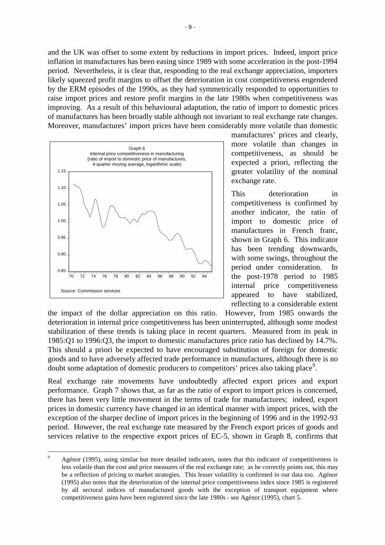
and the UK was offset to some extent by reductions in import prices. Indeed, import priceinflation in manufactures has been easing since 1989 with some acceleration in the post-1994period. Nevertheless, it is clear that, responding to the real exchange appreciation, importerslikely squeezed profit margins to offset the deterioration in cost competitiveness engenderedby the ERM episodes of the 1990s, as they had symmetrically responded to opportunities toraise import prices and restore profit margins in the late 1980s when competitiveness wasimproving. As a result of this behavioural adaptation, the ratio of import to domestic pricesof manufactures has been broadly stable although not invariant to real exchange rate changes.Moreover, manufactures’ import prices have been considerably more volatile than domestic

manufactures’ prices and clearly,more volatile than changes incompetitiveness, as should beexpected a priori, reflecting thegreater volatility of the nominalexchange rate.

This deterioration incompetitiveness is confirmed byanother indicator, the ratio ofimport to domestic price ofmanufactures in French franc,shown in Graph 6. This indicatorhas been trending downwards,with some swings, throughout theperiod under consideration. Inthe post-1978 period to 1985internal price competitivenessappeared to have stabilized,reflecting to a considerable extent

the impact of the dollar appreciation on this ratio. However, from 1985 onwards thedeterioration in internal price competitiveness has been uninterrupted, although some modeststabilization of these trends is taking place in recent quarters. Measured from its peak in1985:Q1 to 1996:Q3, the import to domestic manufactures price ratio has declined by 14.7%.This should a priori be expected to have encouraged substitution of foreign for domesticgoods and to have adversely affected trade performance in manufactures, although there is nodoubt some adaptation of domestic producers to competitors’ prices also taking place9.

Real exchange rate movements have undoubtedly affected export prices and exportperformance. Graph 7 shows that, as far as the ratio of export to import prices is concerned,there has been very little movement in the terms of trade for manufactures; indeed, exportprices in domestic currency have changed in an identical manner with import prices, with theexception of the sharper decline of import prices in the beginning of 1996 and in the 1992-93period. However, the real exchange rate measured by the French export prices of goods andservices relative to the respective export prices of EC-5, shown in Graph 8, confirms that

9 Agénor (1995), using similar but more detailed indicators, notes that this indicator of competitiveness is

less volatile than the cost and price measures of the real exchange rate; as he correctly points out, this maybe a reflection of pricing to market strategies. This lesser volatility is confirmed in our data too. Agénor(1995) also notes that the deterioration of the internal price competitiveness index since 1985 is registeredby all sectoral indices of manufactured goods with the exception of transport equipment wherecompetitiveness gains have been registered since the late 1980s - see Agénor (1995), chart 5.

Graph 6Internal price competitiveness in manufacturing

(ratio of import to domestic price of manufactures,4-quarter moving average, logarithmic scale)

0.85

0.90

0.95

1.00

1.05

1.10

1.15

70 72 74 76 78 80 82 84 86 88 90 92 94


- 10 -

there has been a substantial loss of competitiveness in recent years, mirroring thedeterioration of competitiveness during the 1984-86 period against these same five MemberStates.

The behaviour of export prices suggests that French exporters responded to changes incompetitiveness in a symmetrical way to foreign suppliers of manufactured goods to France.There is also a notable coincidence of the sharp real appreciation of the French franc in 1992and the deceleration in the rise of export prices of manufactures. This likely suggestsstrategic behaviour on the part of French exporters in response to changes in costcompetitiveness, or pricing to market, taking the form of a reduction of their export prices topartially or wholly offset the deterioration in competitiveness10. Agénor (1995) notes thatFrench exporters trade off competitiveness and profitability, and he quotes evidence thatFrench franc-denominated prices are very sensitive to exchange rate movement; thus, in thecase of a franc appreciation, exporters appear to prefer to squeeze profits and to stabilize thelocal price in the destination market rather than increase export prices and endanger theirmarket share.

The more restrained response of import and export prices to changes in price and costcompetitiveness suggests that the competitiveness effects in trade flows may be smaller thansuggested by the actual size of the real appreciation of the French franc in recent years. Thissuggests that the appropriate relative price variable in the empirical work ought to be definednot in terms of the nominal exchange rate and relative costs or prices but by the actual pricesin common currency observed in the market. However, this was possible to do only in theimport equations - see section V and VII below.

,,��F ,PSRUW�SHQHWUDWLRQ��H[SRUW�LPSRUW�UDWLRV��DQG�H[SRUW�PDUNHW�VKDUHV

The internationalization of the French economy over the past thirty or so years is revealed bythe increase in the share of imports in domestic spending. EU and multilateral tradeliberalization since the beginning of the 1970s have played an important role in import

10 Clearly, French exporters may also have chosen to diversify towards high value-added products the

demand for which is less price elastic; to test this hypothesis more detailed data than presently availablewould be required.

Graph 8Changes in relative export prices, French franc in EC-5

(goods and services, 4-quarter moving average,logarithmic quarter-to-quarter changes)

4.50

4.55

4.60

4.65

4.70

4.75

70 72 74 76 78 80 82 84 86 88 90 92 94


Graph 7Terms of trade

Changes in export and import price of manufactures(4-quarter moving average, logarithmic quarter-to-quarter changes)

-0.02

-0.01

0.00

0.01

0.02

85 86 87 88 89 90 91 92 93 94 95 96

Export price Import price


- 11 -

penetration. At the same time, however, competitiveness developments may also have beena factor in import penetration, but, given the wide swings in competitiveness over this perioddiscussed in the previous section, it is likely that competitiveness has played a lesssystematic role11.

Graph 9 presents quantity measures of import penetration for total imports of goods andservices, imports of goods, non-energy imports and imports of manufactures over the period1970 to 1995. The data are ratios of domestic demand in constant (1980) prices. The datashow that the rise in the share of imports in domestic demand has been most rapid in the caseof non-energy and manufactured goods, undoubtedly reflecting the high income elasticity ofdemand for such goods12. The ratio of imports of goods and services in domestic demandhas risen from around 44% in 1970 to around 73% in 1996, an increase of some thirty

percentage points; the ratio ofimports of goods in domesticdemand has risen over the sameperiod by some 26 points to 65% in1996; the share of non-energyimports in domestic demand hasrisen by around 31 points to over55%; and the share of importedmanufactured goods in domesticdemand has risen by around 28percentage points to around 48% in1996. Amongst imports ofmanufactured goods, imports ofhousehold equipment goods is thelargest component, followed bymachinery and transport equipmentwhile current consumption goodswas a smaller category13. The datain Graph 9 appear to suggest that,

despite the increasing openness of the French economy over the past quarter century, the rateof growth of import penetration has slowed down in the 1990s, perhaps reflecting the impactof the slow growth and of the 1993 recession as well as the real appreciation of the Frenchfranc during this period on the demand for imports.

The relative performance in exports and imports, another indicator of competitiveness, ispresented in Graphs 10a and 10b. The data represent 4-quarter moving averages ofexport/import ratios for non-energy and for manufactured goods (Graph 10a) and for fourcategories of manufactured goods in constant prices (Graph 10b). There has been a smoothdecline in the non-energy and manufactures ratios since their peak of 1975. These ratios,

11 It is possible, however, that competitiveness misalignments, which lead to trade hysteresis, have also been

a significant factor in import penetration. In trade hysteresis the loss in competitiveness during the 1990s,for example, may have permanently raised import penetration, as the gains in competitiveness during thedollar appreciation of the early 1980s may have permanently lowered import penetration; see Baldwin(1988). Hysteresis in trade volumes is discussed in sections VI and VIII below.

12 Smoothing the data in the sample 1970:Q1-1996:Q4 yields a trend value of 0.005 for total imports, 0.004for imports of goods, 0.009 for non-energy imports and 0.01 for imports of manufactures.

13 According to data in Agénor (1995), chart 6, household equipment goods represented over 60% ofdomestic demand in 1994, machinery and transport equipment was around 50%, and current consumptiongoods were around 30%.

Graph 9Import penetration

(as percent of domestic demand, 1980 prices, logarithmic scale)

2.8

3.0

3.2

3.4

3.6

3.8

4.0

4.2

4.4

70 72 74 76 78 80 82 84 86 88 90 92 94 96

Total importsImports of goods

Non-energy importsImports of manufactures


- 12 -

while fluctuating around adownward trend, reached anotherpeak in the period of the dollarappreciation during the early1980s. Subsequently, however,coinciding with the dollardepreciation, there was a sharpdeterioration in the export/importratio which lasted until thebeginning of the 1990s. Between1988 and 1991 exportperformance relative to importsstabilized, and since 1991 therehas been some continuous andconsiderable recovery in exportperformance compared to imports,although the export/import ratioremains substantially below itsvalues in the pre-1985 period. Ina manner parallel to the 1985-88period, the franc appreciation ofrecent years could be expected tohave affected negatively theexport/import ratio by reducingexports and encouraging imports.The data suggest that this has notbeen the case. Since the early1990s export performance hasoutstripped import growth withthe result that there has been amarked recovery in theexport/import ratios.

Graph 10b shows that thedeterioration of the export/import ratio for manufactures masks important differences at amore disaggregated level. Of the four categories of imports shown, the most markeddeterioration is in the case of transport equipment and automobiles. While there has beenlittle change in the ratio for household equipment up to the late 1980s, it has subsequentlyshown a modest increase. There was a notable increase in the export/import ratio forprofessional equipment starting in the aftermath of the first oil shock and lasting until thePlaza accords; it subsequently decreased but again since the late 1980s there has been somemodest recovery. The ratio for current consumption goods has also declined in the early partof the sample, but it has stabilized since the beginning of the 1980s and has been virtuallyflat since then. The data in Graph 10b confirm the recovery in the relative export/importperformance since the beginning of the present decade presented in the aggregate data ofGraph 10a.

Graph 10aExport/import ratios, manufactures and non-energy

(4-quarter moving average, 1980 prices)

0.8

0.9

1.0

1.1

1.2

1.3

70 72 74 76 78 80 82 84 86 88 90 92 94 96

Manufactures Non-energy

Graph 10bExport/import ratio in manufactures

(4-quarter moving average, 1980 prices)

0.0

0.5

1.0

1.5

2.0

2.5

3.0

70 72 74 76 78 80 82 84 86 88 90 92 94 96

Current consumption goodsProfessional equipment

Household equipmentTransport equipment and cars


- 13 -

Graph 11 presents alternativeindicators of export performancefor the French manufacturingsector. The data, which is from theOECD14, shows France’s exportmarket growth and her relativeexport performance inmanufactures. Export marketgrowth is a weighted average of allimports, in volume terms, by alltrading partners to which Franceexports; relative exportperformance measures the ratio ofFrance’s export volumes to theexport market. As can be seen inthe Graph, market growthfluctuates widely, consistent withcyclical developments in thetrading partners’ economies.

France’s market share declined sharply in the beginning of the 1980s, then it gained grounduntil the late 1980s when there was another sharp loss of market share in the beginning of the1990s. Since 1993, however, market growth has rebounded significantly. Exportperformance, on the other hand, which contrasts potential to actual exports, shows thatexport performance has deteriorated markedly in the period since the Plaza accords.Notwithstanding the sharp increase in market growth in the post-1983 to the late 1980speriod, France has experienced a trend decline in its export performance in the sense thatactual exports have fallen short of the export market growth. The deterioration wasparticularly pronounced until 1989 and it has continued, albeit at a slower pace, beyond1994.

Developments in market share and in export performance in manufactures may not becorrelated closely with developments in price and cost competitiveness discussed earlier.First, there are long and possibly variable lags between changes in apparent competitivenessand changes in trade flows; secondly, changes in cyclical positions most certainly dominateprice and cost competitiveness in trade flows adjustments; and, thirdly, as noted previously,exchange rate and cost indices of competitiveness disregard the fact that manufactures areimperfect substitutes with other internationally traded and also domestically producedmanufactures and, as a result, they fail to acknowledge pricing-to-market behaviour. As aresult, trade flows adjustments in response to changes in competitiveness and in relativecyclical positions can only be approximated by a dynamic model of the kind used in sectionsV and VII.

,,��G 'HPDQG�GHYHORSPHQWV�LQ�)UDQFH�DQG�DEURDG

The cyclical position of France relative to the rest of the world has been an importantdeterminant of movements in the external accounts; it is also likely that this factor hasplayed a dominant role in the surplus of the 1990s since empirical evidence suggests that the

14 OECD (1996); for a review of the construction of these data and other technical documentation see

Durand et al. (1992).

Graph 11Relative export performance

and export market growth in manufacturing(4-quarter moving average, normalized data, index 1980 = 100)

-2.0

-1.5

-1.0

-0.5

0.0

0.5

1.0

1.5

-3

-2

-1

0

1

2

76 78 80 82 84 86 88 90 92 94

Export performance Market growth (right scale)

Source: Commission services based on OECD data

- 14 -

demand elasticity of trade flows is substantially larger than the relative price orcompetitiveness elasticity. Clearly, small movements in France’s cyclical position againstthe rest of the world can have large effects on the trade balance, such that only unreasonablylarge movements in competitiveness would generate; as will be seen later, the evidencecollected in section IX supports well this hypothesis.

Much of the 1970s to the beginning of the 1980s domestic demand in France and abroaddeveloped in step. Deviations from these trends emerged in the 1980s and becameparticularly pronounced in the 1990s. Graph 12 presents developments in domestic demandin France and in the rest of the world (the exact composition of the world demand variable isdiscussed in section VII, footnote 58), as well as on Commission data for France and the IC-19 and the EC-14 (index of double export weighted national final uses including stocks in1990 prices, annual data), over the period 1980:Q1 - 1996:Q3; the level of the indices isshown in panels (a) and (b), respectively, and the growth differential (4th/4th) betweenFrance and the rest of the world based on the data of panel (a) is shown in panel (c). In thesecond half of the 1980s the level of demand in France grew in parallel with demand abroadand the growth differential fluctuated around zero. However, since 1990 the index fordomestic demand in France has started to deviate significantly from its past trend and to fallbelow the corresponding index for world demand, which has developed broadly in line withits trend of the past decade The Commission data confirm that while the drop in domesticdemand in France was not particularly marked relative to her EC trading partners, it wasnotably greater when measured against the IC-19. The growth differential became

Graph 12Domestic demand in France and the world

(a) Level (1980=100) (b) Relative domestic demand (1991=100)

90

100

110

120

130

140

82 83 84 85 86 87 88 89 90 91 92 93 94 95 96

France World

96

98

100

102

104

106

80 81 82 83 84 85 86 87 88 89 90 91 92 93 94 95 96

Relative to EC-14 Relative to IC-19

(c) Growth differential (France-World, data from panel (a))

-6

-4

-2

0

2

4

6

82 83 84 85 86 87 88 89 90 91 92 93 94 95 96


- 15 -

particularly large from the beginning of 1991 onwards, peaking at 3.3% in 1992:Q215. Thisnegative differential persisted for about 13 quarters until the second quarter of 1994;subsequently, however, growth in world domestic demand outstripped growth in France overmuch of the period between the first quarter of 1995 and the third quarter of 1996. This isthe period when France’s external surplus also developed.

Movements in the external balance are highly correlated with differences in domesticdemand growth between France and the rest of the world. Over the period 1970:Q1 -1996:Q3 the simple correlation coefficient for the non-energy trade balance is -0.61, for themanufacturing trade balance -0.63, and for the current account balance -0.62. Thesecoefficients are suggestive of the substantial dependence of the external accounts on cyclicaldevelopments in France and abroad. Large and sustained deviations of France’s demandgrowth from the rest of the world would tend to reduce (increase) imports and raise (lower)exports, thus contributing to an incipient increase in the external imbalances.

,,,��)DFWRUV�XQGHUO\LQJ�WKH�WUDGH�VXUSOXV�RI�WKH��V

The current account, merchandise trade, and manufacturing trade surpluses of the 1990s havebeen principally the result of trade volume changes rather than price changes. To decomposethe contribution of volume and price effects in movements in these balances, the followingidentity is used:

%W� �3[W ;W��3PW 0W (1)

where B is the balance in question, 3[�and ;�are the export price deflator and the volume ofexports, and 3P and 0 is the import price deflator and the volume of imports, respectively.Totally differentiating (1) and collecting terms, we have the following decomposition:

G%W� �>G;W 3[W��G0W 3PW@��>G3[W ;W��G3PW 0W@

��>G3[W G;W@��>G3PW G0W@ (2)

where the first difference operator is G� �=W��=W��. The first term in brackets is the export andimport volume contribution, respectively, to adjustments in the balance; the second bracketprovides the contribution of the terms of trade changes; and the third and fourth terms arecross-terms of the interaction of volume and price changes. Applying this decomposition tothe French, national accounts, trade data for the period 1990-95 we obtain the resultsreported in Table 316.

Over the period 1990-95 the non-energy trade balance registered a cumulative surplus of FF115.5 billion, and the manufacturing trade balance a cumulative surplus of FF 111.5 billion;thus, the dominant component of the surplus in recent years derives from the goodperformance in trade in manufactures. This is clearly confirmed by the cumulative change inexports of manufactures during this period which, at FF 284.6 billion, were equivalent to

15 Differentials of comparable size have coincided with unstable macroeconomic policies; large demand

growth differentials in France’s favour were recorded during the period 1981:Q4-1982:Q4 of theMitterrand socialist expansion; the Delors reversal of this expansion led to correspondingly large negativegrowth differentials in the period 1983:Q2-1985:Q1.

16 See Mastropasqua and Vona (1988) for a similar decomposition of the US trade balance movements in the1980s.

- 16 -

87.3% of the cumulative change in non-energy exports. The cumulative increase in non-energy imports is also dominated by imports of manufactures which, in the period 1990-95represented approximately 84% of the cumulative change in non-energy imports.

The data in Table 3 show that the largest rise in the surplus occurred in 1992 and also in1993, the years of slow growth and of recession. While there has been some positivecontribution from terms of trade effects throughout the period, these were also particularlyprominent in 1993. It is clear that during 1992-93 export prices were more resilient to thedecline in demand, evidenced by the fall in export volumes, than import prices which likelyresponded more vigorously to the fall in French imports (by FF 50 billion in the case of non-

energy imports and byFF 57 billion in the caseof imports ofmanufactures).

These beneficial effectsof the recession on thetrade balances werereversed, but on amodest scale, with therecovery of the post-1993 period. The non-energy trade balancedeteriorated by some FF8 billion in 1994,notably as a result of thesharp recovery in thedemand for importswhich outstripped therise in exports. Inmanufacturing trade,however, the rise in

exports was significantly larger than the rise in imports with the result that the manufacturingtrade balance has continued to record improvements albeit substantially smaller than those ofthe 1991-93 period.

A notable feature of the data is that the deterioration in price and cost competitiveness duringthe 1990s does not appear to have contributed adversely to trade balance movements. Withthe exception of 1994 and 1995 in the case of manufactures, the terms of trade effects havemade a positive but relatively small contribution to changes in the trade balance in the 1990s.It is possible to note that should competitiveness have remained at the same level as in thelate 1980s the potential improvement in France’s trade balance, ceteris paribus, would nothave been affected significantly. On the other hand, had domestic demand remained at itstrend value during the second half of the 1980s, there likely would have been, ceteris paribus,no improvement in France’s external performance. Finally, together with the evidencesuggested in Graph 11, it is likely that had export performance kept up with France’sinternational market growth, certainly in the post-Plaza accords period as a whole and morespecifically during the post-1989 period, France’s external performance would have beenmarkedly better.

Table 3Decomposition of non-energy and manufacturing trade balance

(in billion of francs)

1990 1991 1992 1993 1994 1995 Cumulative

Non-energy trade

Change in trade balance 2.3 16.6 47.8 43.0 -7.8 13.6 115.5

due to: ([SRUW�YROXPH 56.7 45.8 57.5 -15.8 80.3 101.4 325.9

,PSRUW�YROXPH 67.0 29.2 11.6 -49.7 90.9 85.3 234.4

7HUPV�RI�WUDGH 11.7 0.1 3.1 10.3 3.0 2.4 30.6

2WKHU 0.9 -0.2 -1.5 2.2 -1.1 -1.6 -1.3

Residual 0.0 -0.1 -0.3 -3.4 -0.9 -0.9 -2.5

Trade in manufactures

Change in trade balance -0.8 23.0 39.3 39.3 4.2 6.5 111.5

due to: ([SRUW�YROXPH 50.2 40.1 44.7 -31.5 87.9 93.2 284.6

,PSRUW�YROXPH 60.3 18.1 9.4 -56.7 81.1 84.6 196.8

7HUPV�RI�WUDGH 8.6 0.5 4.7 19.4 -2.5 -2.0 28.7

2WKHU 0.7 0.3 0.7 2.8 -0.3 -0.1 -4.1

Residual 0.0 -0.2 -1.4 -2.5 -0.2 0.0 -4.3

The entries in the table are based on the decomposition, according to equation (2), discussed inthe text; “Other” refers to the cross-terms in equation (2) of the text.

Source: Calculations based on original INSEE data; see Annex A.

- 17 -

The decomposition of Table 3 is only indicative of the behavioural adjustments in export andimport functions in response to the competitiveness and output shocks which have occurredin recent years. An exact quantitative evaluation requires estimates of the export and importfunctions with respect to the determinants postulated by economic theory. Moreover, as theimpact of these shocks on trade flows is likely not instantaneous, it is essential to obtainestimates of the lags which typically characterize adjustments in trade flows17. Finally, onemethod of uncovering the sources of the external surplus of recent years would be throughthe use of simulations. For these reasons, a more thorough econometric estimation approachis undertaken in subsequent sections.

,9��(FRQRPHWULF�PHWKRGRORJ\�DQG�PRGHOOLQJ�VWUDWHJ\

This section reviews the main methodological issues that impinge upon the specification andeconometric estimation of models of trade flows.

,9�D�6SHFLILFDWLRQ�RI�WUDGH�IXQFWLRQV

Conventionally, empirical analysis of trade flows has been carried out through a partial-equilibrium model based on the hypothesis of imperfect substitution between foreign anddomestic goods. The model assumes that, in a simplified two-country world, each countryproduces a single tradable good that is an imperfect substitute for the good produced in theother country. The simplest and most widely used procedure for estimating aggregate exportand import demand functions in this framework18 is based on the Marshallian demandfunction.

TThhee ggeenneerraall ffuunnccttiioonn ffoorr aaggggrreeggaattee iimmppoorrttss hhaass tthhee ffoolllloowwiinngg tthheeoorreettiiccaall ffoorrmm::

0G� �)�<��3P��3G� (3)

I�!��I��I�!��

where�0G�= volume of imports demanded, 3P = price of imports,�3G = domestic price ofimport-competing goods, and < = real domestic economic activity; IL are the expectedpartial derivatives with respect to the Lth argument. Equation (3) suggests that the demandfor imports is determined by the level of expenditure or income (or another scale variablethat captures domestic demand conditions) and by the price of imports and domesticsubstitutes measured in the same currency19. With homogeneity of degree zero in prices andnominal income, consistent with absence of money illusion, equation (3) can be re-writtenwith a relative price term:

0G� �)�<��53� (4)

17 One important effect, for example, is associated with the lagged response of volumes and the

instantaneous response of prices in the event of competitiveness shocks, giving rise to J-curve movementsin external balances; however, examination of such effects is beyond the scope of the present study.

18 For an excellent but somewhat dated survey of the literature on imperfect substitutes and perfectsubstitutes models in international trade, the latter implying the law of one price, see Goldstein and Khan(1985).

19 This is in accordance with conventional demand theory that assumes the consumer to maximize utilitysubject to a budget constraint and, for the case in which the importer is a producer, to maximizeproduction subject to a cost constraint; see Goldstein and Khan (1985).

- 18 -

I�!��I��

Correspondingly, the general function for aggregate exports has this theoretical form:

;G� �)�<Z��3[��( 3Z� (5)

I�!��I��I��!��

where ;G = volume of exports demanded by foreigners, <Z = world economic activity inconstant prices,� 3[ = price of exports, 3Z = foreign competitors’ prices in the country’sexport markets and ( = nominal exchange rate in units of foreign currency per unit of homecurrency; IL�are the expected partial derivatives of the export function with respect to the Lthargument. According to equation (5), the foreign country’s demand for exports is a functionof its real income or expenditure, of the price of the domestically produced substitute goodand of the price of the foreign competing good. As in equation (4), equation (5) can be re-written with a relative price term (3[�( 3Z��which can be viewed, alternatively, as the termsof trade or the real exchange rate. The use of this variable imposes the constraint ofhomogeneity in prices which is not testable.

;G� �)�<Z��3[�( 3Z� (6)

I�!��I��

The supply side function of the imperfect substitute model postulates that the quantitysupplied is a positive function of the own price and a negative function of the price ofdomestic goods in the exporting or importing country. The price elasticity of supply is oftenassumed to be infinity or at least largely independent of the quantity of trade. This allowsestimation of a single equation, reduced form, model by ordinary least squares since exportand import prices can be considered as exogenous. As stressed by Goldstein and Kahn(1985), this assumption appears more plausible for the case of imports rather than for thecase of exports since for a single country it is more difficult to increase its supply of exportswithout an increase in costs and thus in prices compared to the rest of the world .

Another basic assumption of the model is that exporters and importers are always on theirdemand schedules so that demand always equal the actual level of trade flows. However, itis generally recognised that imports and exports do not immediately adjust to their long-runequilibrium level, following a change in any of their determinants. To take into account theslow reaction of the economic agents to changes in the explanatory variables due toadjustment costs, inertia, habit or lags in perceiving changes, a simple first-order partial-adjustment mechanism has often been included in the equations, permitting a short-runadjustment towards the long-run equilibrium. More generally, the relaxation of theequilibrium hypothesis in the general function has usually been achieved by specifying adynamic model within the framework of a general distributed model with geometricallydeclining weights (the Koyck model) or, following Almon, by assuming that distributed lagcoefficients lie on an exact polynomial curve20. 20 One of the drawbacks of the partial-adjustment model is that it imposes the same geometrically weighted

lag distribution on both the real income and relative price variables, while trade flows are known to

- 19 -

,9�E��(FRQRPHWULF�PHWKRGRORJ\

Most of the empirical work on the OLS estimates of aggregate and disaggregated trade flowshas used variables in (log) levels rather than first-differenced or otherwise filtered data. Yet,in the case of non-stationarity21 of the time series involved in the analysis, estimatedcoefficients are likely to be inconsistent. In addition, the assumption of conventionalasymptotic econometric theory does not hold and the use of standard statistic tests is notvalid. Most often, to cope with the presence of autocorrelation in the residuals (arbitrarilyinterpreted as indicative of autoregressive errors) that often arises when quarterly data ofvariables in level are used, a re-estimation with Cochrane-Orcutt or other serial-correlationcorrection methods has been carried out. Yet, this procedure is justified and valid only inpresence of a “common factor”, otherwise it will give rise to inconsistent estimates22.

In some cases, to avoid obtaining inference from spurious regressions23 and problems in theerror process, only first-differenced time series have been employed in the estimation.However, such a modelling is valid only if the time series are not cointegrated. If the seriesare cointegrated, a model with only differenced variables will be misspecified and theestimates will be biased and inconsistent. Furthermore, such models do not includeinformation about the long-run equilibrium relationship between the variables.

The parametric error-correction methodology avoids the shortcomings of the conventionalleast squares regression. We have examined aggregate trade demand equations using thefollowing two-stage procedure. First, we have tested and estimated the cointegratingrelationship, by applying the Johansen maximum likelihood methodology to the aggregatenon-energy and manufacturing import and export functions derived from the imperfectsubstitution model. Then we have imposed this long-run result as an error correction

respond more rapidly to income changes than to price changes. Moreover, this model arbitrarily imposesrigid conditions, such as a specific pattern to lag structure estimates.

21 We adopt, as usual, the notation that a non-stationary variable ;t is integrated of order d (i.e. ,>G@� if itrequires to be differenced d times to become stationary �,>�@�, i.e. to remove the non-deterministic trend.Alternatively, if adding a time trend is sufficient to induce stationarity, the series is defined to be trendstationary. If ;W�∼�,>�@� then ∆;W�∼�,>�@, and when the data are in logarithms these changes (i.e. ∆ORJ;W� ORJ;W��ORJ;W�� ORJ�;W�;W�� are growth rates.

22 More formally, a linear regression equation relating a variable <W to its own lagged value and to the currentand lagged values of a regressor variable, ;W��<W�� α<W��;W��δ�;W��W� where |α|�� and �W�∼��σ�

��can be transformed into: <W� �α/\W��;W��δ�;W��W using the lag operator / (where /<W� �<W��RU��α/�<W� ��δ�/�;W��W� If the parameter δ� ��α� , then the last equation becomes: ��α/�<W� � ��α/�;W� � �� W where ��α/� is the common factor of the terms involving <W� and ;W� and implies anautoregressive error process. In fact, dividing both sides of the last equation by the common factor, weobtain: <W� ��;W��µW��α/�� ;W��εW where εW� ��W��α/�� or εW� ��εW��W, which represents the firstorder autoregressive process generating the error term. Only in this case (that is when the condition δ� ��α� holds) the use of Cochrane-Orcutt transformation (which, indeed, imposes a common-factor restrictionassuming an $5 error process) for removing a first order autocorrelation in the residuals may be optimal,and serial correlation can be considered a convenience rather than a nuisance, because it allows estimatesof only three parameters �α��and�σ�� instead of the four parameters �α��δ�and�σ�� of the first model;see Hendry and Mizon (1978).

23 Spurious regressions refer to relationships between the variables in an equation only due to correlatedstochastic time trends in the data.

- 20 -

mechanism to a single-equation-error-correction-model �6((&0�24 and we have estimatedthe short-run dynamics.

The explicit 6((&0 specification of the trade equations is:

∆PW�� $�/�∆PW��%�/�∆\W��&�/�∆USW��θ>PW��P W��@��W(7)

∆[W�� $�/�∆[W��%�/�∆\ZW��&�/�∆UHHUW��ϕ>[W��[ W��@��εW (8)

where $�/��%�/� and &�/� are finite polynomials and ∆ is the first difference operator. Theterm in squared brackets is the error-correction term, that is the deviation of actual importand export demand, PW and [W, from the long-run equilibrium or cointegrating relation, P Wand [ W, respectively. The equations have been estimates in log functional form, so that thecoefficients are elasticities.

,9�E��8QLW�URRW�DQDO\VLV

Before applying the cointegration and the error-correction methodology mentioned above itis necessary to determine the time-series properties (i.e. the order of integration) of eachvariable, by testing whether they are stationary or they include a stochastic trend25. Weemployed the most commonly used Dickey-Fuller (DF) and augmented Dickey-Fuller (ADF)univariate tests of the null hypothesis of a unit root in our observed time-series, against thealternative that the process is stationary26. In computing the ADF test we have employed upto four lags to remove residual autocorrelation in the quarterly data used here.

The results of the two tests are reported in Annex A and show that at the 5% significancelevel the null hypothesis of a unit root in the series under consideration cannot be rejected atleast in the sample period under examination (1970:Q1-1996:Q4)27. The only exception isthe real effective exchange rate defined in terms of unit wage costs in manufacturing against23 industrial countries and 20 industrial countries which appear to be ,��.

To examine the data for the presence of a second unit root, the DF and ADF tests wereapplied to the first differences in logs of the time series. The results indicate that thepresence of a second unit root is easily rejected; therefore, the first difference of all theseries under consideration is stationary, thus confirming that the series are likely to be ,>�@ in(log)level. Hence, with usual caveats arising from the low power (the tendency to under-reject the null of non-stationarity when it is false) and poor size (over-rejecting the nullhypothesis when it is true) of the tests in finite sample, and the problem of “near

�� The 6((&0 can be considered as a generalization of conventional partial adjustment model widely used

in the specification of import and export demand functions, and is consistent with optimizing behaviour ofeconomic agents in a dynamic environment.

25 A stochastic variable Yt generated by a first-order autoregressive process <W� �ρ<W�� µW is stationaryifρ⟨��. A stationary time-series tends to return to its mean value and fluctuate around it with a finitevariance.

26 For a survey on new extension of the Dickey-Fuller procedure and other alternative non-parametric tests,such as Phillips and Perron test, see the introduction of Banerjee and Hendry (1992) and the followingthree articles in the special issue of the Oxford Bulletin of Economics and Statistics.

27 In fact, the order of integration of a time-series is sensitive to the period over which the tests areperformed. The degree of integration is not necessarily an intrinsic property and could change overhistorical periods.

- 21 -

observational equivalence”28, it seems reasonable to carry out the analysis assuming that allthe variables in our information set, with the exception of the real exchange rates mentionedpreviously, are non-stationary, i.e. they contain a stochastic trend over the 1970:Q1-1996:Q4sample. Accordingly, standard asymptotic theory can not be applied estimating equationscontaining variables in level because the properties of the series do not satisfy the classicalassumptions of constant mean and variance which, on the contrary, evolve with time;standard errors of the parameters will be biased and could give rise to “spurious” regressionsin the non-cointegrated case29.

The same problem could arise if the levels of non-stationary variables were introduced inregressions that are formulated in differences (as it is done modelling an unrestricted errorcorrection model). In fact, if the regression is to have stationary residuals in order to avoidspurious regression when the variables are integrated, there must exist at least one linearcombination of the levels of variables which is stationary30. If it does exist, the variables aresaid to be cointegrated and the linear combination can be interpreted as a long-runequilibrium relationship which holds apart from a stationary stochastic error representingshort-run deviations. Therefore, we have first tested for the presence of cointegration amongthe variables of interest and then formulated the error-correction dynamic model.

,9�E��&RLQWHJUDWLRQ�DQDO\VLV

The cointegration methodology31, first proposed by Granger (1981), Engle-Granger (1987)and extended by Johansen (1988), is now commonly used in the construction of single-equation dynamic models. In our case, cointegration has been used to evaluate the long-runstationary steady-state between the level of imports and exports and their theoretically mostimportant determinants.

When there are more than two ,>�@ variables under consideration, as in our case, the mostcommon cointegration analysis proposed by Engle and Granger (EG), based on a OLS staticregression and on the DF and ADF cointegration tests of the residuals (using correct criticalvalues), has proved to be inefficient32. In finite samples the EG method is sensitive to the so-called direction normalisation rule, that is to the specific choice of the endogenous variableto put on the left-hand side of the equation. The method also ignores the possibility of morethan one cointegrating vectors when more than two variables are included in the analysis. Inaddition, the ADF test for cointegration imposes an implicit common factor restriction on the

28 In finite samples, any trend-stationary process could be approximated arbitrarily well by a unit root

process and vice versa; in addiction, the usual tests are not able to reject the null hypothesis if thedeterministic trend of the series has a single break. For this and other criticisms see Campbell and Perron(1991).

29 On this issue see Granger and Newbold (1974), Dickey and Fuller (1979) and Engle and Granger (1987).30 In a bivariate case, two variables �;��<� are said to be cointegrated of order one, i.e. &,>��@, if they are

individually ,>�@, but some linear combination (i.e. ;�α<) of the two is ,>�@; see Engle and Granger(1987).

31 Cointegration is a statistical property that describes the long-run behaviour of economic variables andprovides a formal underpinning to the use of the error-correction model (ECM) as it has beendemonstrated in the Granger Representation Theorem. A treatment of this topic is in Banerjee et al.(1993).

32 Stock (1987) has shown that if each variable is ,>�@ and if there is a cointegrating vector such that thelinear combination is ,>�@, then the OLS estimators of this vector are consistent and converge inprobability faster than in ordinary case, that is they are "super consistent". On the contrary, Banerjee etal. (1986) found with Monte Carlo simulations and asymptotic approximations that in finite samples theOLS procedure can lead to some bias which decreases only slowly as the sample size increases.

- 22 -

long-run model; if the restriction is not valid, the test loses power33. In view of theseconsiderations, we presently test the cointegration hypothesis using the more powerfulJohansen FIML (Full-Information Maximum Likelihood) approach in the multivariateframework.

The Johansen procedure is based on maximum likelihood estimation of a vectorautoregressive (VAR) system. It is a method for estimating both the distinct cointegratingvectors which may exist within a set of variables and for carrying out a range of statisticaltests. Given a 1[� vector of non-stationary ,�� variables ;W and considering a VAR modelof order p, with Gaussian errors, we obtain34:

;W� �&W��Π�;W��ΠS;W�S��εW (9)

where &W��is an 1×� vector of deterministic components (such as constants, dummies or driftterms), ΠL� � L� ��p are 1×1 parameter matrices, εW is a vector of white noise errors withcovariance matrix >0 and W� ��7�

By re-parametrizing35, the VAR can be transformed into a reduced-form error-correctionmodel or vector error-correction model (9(&0), in which we can directly distinguishbetween the effects related to the short-and long-run variation in the data:

∆;W� �&W��∑ΓL∆;W�L��Π�;W��εW (10)

where

ΓL ��Π�L��Π,��Π ��ΠL��ΠS��,��L ��S��

When there are more than two variables in the VAR, it is not necessary for all of them tohave the same order of integration. However, for every stationary variable included in theVAR, the number of cointegrating relationship will automatically increase correspondinglybecause each ,�� variable forms a cointegration relation by itself36. What really matters isthat the variables on both side of the 9(&0��were jointly “balanced” in order to preserve theassumption of a stationary (zero mean) error term εW�The matrices of parameters ( Γ, C and Π ) are estimated using maximum likelihood method.The choice of deterministic components (constant, trend) to introduce in the 9(&0,restricted to enter the cointegration space or unrestricted, influences the distribution of thecointegrating tests. In the formulation of the system the lag-length of the ∆;W�L should be highenough to assure a white noise disturbance vector εW. In the reduced-form model, which islikely to be heavily overparametrized, the short run dynamics is given by the elements ofmatrix ΓL. The estimates of these matrices is intended to correct the variation in ;W�related tothe short run. The cointegration test involves determining the rank of the matrix�Π, which

33 See Banerjee et al. (1993).34 Contrary to the approach of Engle and Granger, in this multivariate approach all the variables are

explicitly endogenous so it is not necessary to make any preliminary and arbitrary normalization.35 Adding and subtracting various lags or simply using the first-difference operator ∆, defined as ∆;W� �;W��

;W��. This re-parametrization leaves all the properties of the residual unchanged.36 As stressed by Harris (1995) “stationary variables might play a key role in establishing a sensible long-run

relationship between non-stationary variables, especially if theory a priori suggests that such variablesshould be included”, p. 80.

- 23 -

corresponds to the number of its non-zero eigenvalues, which contain information on thelong-run properties of the ;W variables. Therefore, the magnitude of the eigenvalues �λL�provides information on the presence of a cointegrating relation. For the eigenvectorscorresponding to the non-stationary part of the model (or “common trends”), λi ≅ 0 for L� �U��Q. In the situation where the components are non-stationary and integrated of order 1,the rank of the Π matrix determines the cointegration properties of ;W, that is the number ofcointegrating vectors in the system.

There can be three different cases for the rank of Π which are of particular importance37:

1) If U� �Q, that is the matrix�Π has full rank, this implies that all the n variablesin X are stationary.

2) If U� ��, that is Π� is a null matrix, this implies that no cointegrating vectorexists because all linear combination of ;�are ,>�@� In this case the reduced-form becomes a model of only differenced variables.

3) If ��U��Q, that is the matrix Π�has a reduced rank, then there are �Q�U� linearcombinations of ; which act as a common stochastic trend, and U�cointegratedlinear combinations.

Summing up, the hypothesis of cointegration is formulated as the hypothesis of reduced rankof the coefficients matrix Π. If this holds, the latter can be decomposed as: Π αβ¶ underthe Johansen ML procedure, where�� is the Q�×�U matrix of cointegrating vectors (each rowβL is a cointegrating vector) and α is the Q�[�U matrix of “weighting elements”. The matrix αcontains the adjustment coefficients which represent the feedback effects fromdisequilibrium to the dependent variables. In case of only one cointegrating vector, if a givencolumn of α�is not different from zero, except for the first entry, single-equation estimationof the relation will not lead to loss of information on cointegration and dynamic behaviour.This is because the right-hand variables can be considered weakly exogenous for the variableof interests38.

The stationary relations �¶;W�� are referred to as the cointegrating relations. The estimate ofß’ is obtained by solving an eigenvalue problem, whose solution is represented by theeigenvectors �L and the eigenvalues λL. When there is more than one cointegrating vector themultivariate model determines the cointegration space, instead of the individual vectors, andthis makes the analysis more complicated due to the difficulties of interpreting thecointegration space39.

For testing cointegration, the Johansen approach is based on sequential likelihood ratio testof the null hypothesis of Q�U unit roots against the alternative of Q�U�� unit roots. Twodifferent tests have been developed40:

1) The trace statistic test: λWUDFH� ��7�∑�L U��OQ��λL�� , r=0, 1,..n-1 were λL are theordered largest eigenvalues.

37 See Johansen and Juselius (1990) for a detailed exposition.38 See Banerjee et al. (1993).39 See Juselius (1992).40 The test strategy is the multivariate analogue of the Dickey-Fuller (DF) test. Critical value for these tests

have been tabulated by Johansen (1988), Johansen and Juselius (1990), Osterwald-Lenum (1992).

- 24 -

2) The max statistic test: λPD[� � �� 7OQ��λU�� which is based on the largesteigenvalue. In this case, as noted before, a small value of�λL implies that the unit roothypothesis cannot be rejected at the UWK level of significance, as in the case of scalarunit root tests41.

The trace test has been found to show more robustness to both skewness and excess kurtosisin the residuals than the λPD[ test42. As usual, if λWUDFH� or��λPD[ exceeds the critical value, thenull can be rejected in favour of the alternative. It should also be stressed that testing forcointegration by investigating for the number of U linearly independent columns in Π isequivalent to testing that the last �Q�U� columns of α�are insignificantly small.

In this multivariate framework, after testing hypotheses on the number of cointegratingrelationships, we can also test certain linear restrictions on �. This involves testingrestrictions of the form β� �+φ where + is the restriction matrix and� φ is the parametermatrix. To carry out this test the statistics: Q�∑U�L ��OQ�[��λ ��λ�] can be used; here λ

refers to eigenvalues derived under the parameter constrained and λ refers to unconstrainedeigenvalues. This is a likelihood ratio and the statistic is asymptotically distributed as χ�under the null.

9��'HWHUPLQDQWV�RI�LPSRUWV��6SHFLILFDWLRQ�DQG�HVWLPDWLRQ�UHVXOWV

The explicit restricted form of equation (4), the long-run demand for imports, has thefollowing form:

0W� �α��β ''2�W��γ 53W (11)

where all data are in logarithms and 0 = volume of imports, ''2� = domestic demandincluding stocks, and 53 is the relative price term, 53� �30�3'��where�3' = domestic priceof import-competing goods, and 30 = price of imports. The restricted equation assumes thatthe individual price terms have identical but opposite in sign coefficients, a restrictiongenerally supported by the data.

Equation (11) is assumed to represent the cointegrating, long-run, relationship betweenimports and their determinants. The short-term dynamics of adjustment of actual imports tothe level consistent with the long-term determinants is represented by an error-correctionprocess, an explicit form of equation (7), of the following form:

∆0W� �D��ΣDL:W�M��θ>0W��α��β ''2�W��J 53W��@

� �D��ΣDL:W�M��θ>(5W��@ (12)

where : is a vector of independent variables in first-difference form lagged j quarters whichincludes also values of the dependent variable starting from t-1 and lagged j quarters, θ is theerror-correction coefficient, and (5 is the error term from the cointegration vector which, for

41 In the trace test, the null hypothesis is that the number of cointegrating vectors (U) is less than or equal to Q

(where Q� � �� 1� against a general alternative that U� !� Q; in the maximum eigenvalue test thealternative hypothesis is explicit �U� �Q��.

42 See Cheung and Lai (1993).

- 25 -

cointegration, must be stationary. θ must be negative in order that values of imports larger(smaller) than the prediction of the cointegrating equation lead to reduction (increase) incurrent imports; thus, a negative value of θ ensures stability. The model is deliberatelyparsimonious in the choice of variables in order to test strictly the predictions of economictheory and the value of the error-correction approach to modelling the demand for imports.

The estimation strategy follows the two-step procedure. First, the cointegration vector (11)is obtained with the Johansen procedure through a search process based on the Pantulaprinciple43; as a result, only a constant term is included in the cointegration equation as wellas in the dynamic model; secondly, the error term of the cointegration vector is used as anindependent variable in the dynamic regressions (12). The data are all in logarithms, and themnemonics used in the regressions reported in Table 5 below are as follows: ''2�� =domestic demand including stocks (1980 prices); 303*'3 = ratio of import to GDPdeflator; 303''� = ratio of import to domestic demand deflator; I0304 = imports ofmanufactures (1980 prices); and 30'0$18 = ratio of import price to domestic price of

manufactures.

Two sets of regressionsare reported, equation (I)where the dependentvariable is non-energyimports and equation (III)where the dependentvariable is imports ofmanufactures.Furthermore, equation (I)is estimated with the ratioof the import to the GDPdeflator as the relativeprice term, and equation(II) with the ratio ofimport to the domesticdemand deflator as the

relative price term.

The results of cointegration tests, based on the Johansen method with a lag order of three in9(&0, are reported in Table 4. The test statistic is λWUDFH discussed previously. The Pantulasearch suggested that the long-run equations had intercepts but there was no trend in therelationship between import demand and its determinants; this specification not onlydescribed the data best but it also likely yielded Gaussian errors44. The results confirm thatthe variables in question are cointegrated, and in all cases the cointegration vector is unique.The null of no cointegration is rejected at the 99% level of significance in the case ofequations (II) and (III), and at the 95% level of significance in the case of equation (I), at thelargest eigenvalue. The somewhat lower level of significance at which cointegration issupported by the data in the case of the non-energy equation defined over the relative price ofthe ratio of import to the GDP deflator points to the presence of some instability, an issue towhich we will return once more in section VI. Nevertheless, the results support the

43 See Harris (1995), p. 97, on this.44 An alternative specification, where it was postulated that the long-run equation was defined over no

intercept or trend, yielded essentially robust results but unreasonably large elasticity estimates.

Table 4Imports, domestic demand and relative prices

Johansen likelihood ratio tests for cointegration, trace test

Nocointegration

At mostone vector

At most twovectors

Sample 1970:Q1-1996:Q3

(LJHQYDOXH ��

Non-energy imports, equation (I) 31.07* 9.10 2.46(LJHQYDOXH ��

Non-energy imports, equation (II) 37.45** 12.14 3.62(LJHQYDOXH ��

Imports of manufactures, equation(III)

39.59** 12.16 3.76*

The null hypotheses are that there is no cointegration, that there is at most onecointegration vector, and that there is at most two cointegration vectors; the 5% criticalvalues of the likelihood ratio statistic at the three largest eigenvalues reported for eachequation in the Table are 29.68, 15.41 and 3.76; the 1% critical values are,correspondingly, 35.65, 20.04 and 6.65; * (**) rejects the null at the 5% (1%) level ofsignificance; equations (I), (II), and (III) refer to those in Table 5.

- 26 -

hypothesis that there is a long-term relationship between imports, domestic demand andrelative prices, as postulated by economic theory, and that this relationship is unique. Thiscointegration vector can, therefore, be interpreted as representing the long-term demand forimports45.

The estimated long-run demand for imports is shown in the upper panel of Table 5. The firstadjustment weight suggests that a 1% deviation of actual imports from their predicted valuecauses an adjustment of non-energy imports equal to around 55% each quarter; in the case ofimports of manufactures, this adjustment is even faster, around 70% of the deviation in each

45 Cointegration is confirmed by unit root tests for the residuals of the estimated vectors. The ')�($')��

statistic for the error of equation (I) is -5.05 (-4.51); for the error of equation (II) it is -4.72 (-4.74); andfor the error of equation (III) it is -5.12 (-4.93). The critical value of the test statistic at the 99% (95%)level of significance is -3.50 (-2.89).

- 27 -

Table 5

Demand for importsRestricted cointegration/error correction model for imports, domestic demand, and relative

import/domestic price, 1970:Q1-1996:Q3(equations (I)-(III), standard errors in parentheses)

Non-energy imports Imports of manufactures

(I) (II) (III)

Cointegrating vector

DDO2 2.253 2.142 DDO2 2.357(0.051) (0.070) (0.055)

PMPGDP -0.201 - PMDMANU -0.404(0.066) (0.142)

PMPDD2 - -0.358 -(0.095)

Constant 18.806 16.949 Constant 19.988

ì1 -0.536 (0.155) -0.556 (0.142) ì1 -0.691 (0.145)ì2 -0.034 (0.057) -0.038 (0.053) ì2 -0.089 (0.048)ì3 0.057 (0.122) -0.018 (0.108) ì3 0.068 (0.084)

Short-term adjustment model

θ -0.272 -0.308 θ -0.519(0.126) (0.119) (0.120)

d(DDO2(-1) - 0.187 d(IMPMQ(-1)) 0.120(0.260) (0.091)

d(DDO2(-2)) 0.275 0.250 d(IMPMQ(-2)) 0.137(0.251) (0.253) (0.090)

d(DDO2(-3)) 0.380 0.392 d(DDO2(-3)) 0.456(0.247) (0.247) (0.285)

d(PMPGDP(-2)) -0.227 - d(PMDMANU(-2)) -0.209(0.132) (0.181)



d(PMPDD2(-2)) - -0.281 -(0.135)

d(PMPDD2(-4)) - -0.400 -(0.125)

Constant -10.213 -10.425 Constant -20.729(4.606) (4.031) (4.815)

R² 0.284 0.304 R² 0.311SER 0.024 0.024 SER 0.027DW 1.839 1.966 DW 1.922

Jarque-Bera χ² (2) 2.369 2.240 Jarque-Bera χ² (2) 1.279F(ARCH(4)) 0.791 (0.50) 1.001 (0.41) F(ARCH(4)) 1.200 (0.32)F(RESET) 0.813 (0.54) 1.119 (0.36) F(RESET) 1.277 (0.28)F(HET1) 1.174 (0.32) 0.463 (0.92) F(HET1) 1.086 (0.38)F(HET2) 1.032 (0.44) 0.367 (1.00) F(HET2) 0.909 (0.61)F(AR(4)) 1.705 (0.16) 0.954 (0.44) F(AR(4)) 1.674 (0.16)

ãi refers to the value of the adjustment coefficient in the import function entering the first, the second(DDO2) and third (relative price) equation, respectively, in the VAR; θ is the error correction term; d(Z)is the first-difference operator for Z; R² is the adjusted R²; SER is the standard error of the regression;DW is the Durbin-Watson statistic; the Jarque-Bera statistic for the normality of the residuals,distributed as χ² with two degrees of freedom, has a 95% critical value of 5.99; F(ARCH(4)) of lag order4 is the F test for autoregressive conditional heteroscedasticity (probability in parentheses); F(RESET)is Ramsey’s F statistic for specification error run on five fitted terms; F(HET1) is White’s F test forheteroscedasticity, no cross terms; F(HET2) is White’s F test for heteroscedasticity, with cross terms;F(AR(4)) is the LM test for serial correlation of order 4; sample 1970:1-1996:4.

- 28 -

11.0

11.2

11.4

11.6

11.8

12.0

12.2

12.4

10.8

11.0

11.2

11.4

11.6

11.8

12.0

12.2

12.4

74 76 78 80 82 84 86 88 90 92 94 96

Long-term Actual Simulated (right scale)

Graph 13aNon-energy imports: Long-term, actual, and simulated

(equation (I), logarithmic scale)

11.0

11.5

12.0

12.5

11.0

11.5

12.0

12.5

74 76 78 80 82 84 86 88 90 92 94 96


Graph 13bNon-energy imports: Long-term, actual, and simulated

(equation (II), logarithmic scale))

10.5

11.0

11.5

12.0

12.5

10.5

11.0

11.5

12.0

12.5

74 76 78 80 82 84 86 88 90 92 94 96


Graph 13cImports of manufactures: Long-term, actual, and simulated

(equation (III), logarithmic scale)

- 29 -

quarter. The remaining adjustment weights are of negligible value, implying thatdisequilibrium in the import demand equation causes adjustment only in that equation alone,supporting the hypothesis that domestic demand and the real exchange rate are weaklyexogenous for the parameters of the conditional import equation and also supporting thesingle-equation estimation procedure followed here46.

The estimated long-run import equations, where the cointegration space is restricted to onevector, have the following form:

,03121(� �� ''2�� 303*'3 (13)

,03121(� �� ''2�� 303''� (14)

,0304� �� ''2�� 30'0$18 (15)

where ,03121( = non-energy imports and ,0304 = imports of manufactures. The resultssuggest that imports of non-energy goods and imports of manufactures are almost equally, andhighly, elastic with respect to domestic demand, with the elasticity ranging from around 2.2 inthe case of non-energy imports to close to 2.4 in the case of imports of manufactured goods.This high elasticity explains the rapid rise of imports in domestic demand, shown by thepenetration ratios of Graph 947; this is a property of the sample period characterized by tradeliberalization and by rapid growth in intra-European and world trade. The estimates reportedpresently compare well with those of Germany (1.86) and that of the US (2.04) obtained inCarone (1995) for total imports of goods. In contrast, estimates reported in the Banque deFrance (1996) for imports of manufactures are substantially lower, and they are eitherrestricted to or estimated at around unity, but the equation includes an import penetration termwhich undoubtedly biases the estimate of the elasticity with respect to demand downwards.This is clearly a model-specific matter, reflecting different modelling strategies, choice ofvariables and sample size, as is also the case in Bonnaz et Paquier (1993) who estimate anelasticity for imports of manufactures with respect to domestic demand equal to unity and along-term price competitiveness elasticity of -0.7. Capet et Gudin de Vallerin (1993), from thesample 1970:Q1-1988:Q4, obtain a domestic demand elasticity of imports of manufacturesalso of unity and a price competitiveness coefficient of -0.81; their equation includes a relativecapacity utilization term and a time trend too48.

Similarly, the long-term demand elasticity estimates reported in Goldstein and Khan (1985) areobtained from earlier samples ending at the latest in 1980 and are undoubtedly contaminated

46 The exogeneity status of variables is not presently investigated further. For an overview of the three main

concepts of exogeneity (weak, strong and super) and their importance for conducting valid inference as wellas forecasting and policy analysis in a conditional econometric model see Engle, Hendry and Richard(1983), and Ericsson and Irons (1994).

47 Note also in this respect that a long-run elasticity of imports with respect to domestic demand exceedingunity is not admissible since it would imply that imports would ultimately dwarf domestic demand andoutput. However, it is quite conceivable, as the empirical evidence shows, that specific samples such as theone used here may be characterized by high values of this elasticity consistent with the rapid rise in importpenetration.

48 Capet et Gudin de Vallerin (1993) find two cointegration vectors for imports; although both vectors areeconomically meaningful, the presence of cyclical variables in the long-term relationship is problematic anddifficult to defend - see also footnote 51. The estimated demand elasticity in the present parsimoniousmodel may be a mixture of demand and of other factors which are not explicitly articulated here; as apossible alternative specification see the estimates in Temple and Urga (1997) where, on UK manufacturingdata, the demand elasticity is unity but the elasticity with respect to an OECD exports/domestic productionvariable is 1.55.

- 30 -

by, and reflect the importance of, restrictions in France’s trade during that time. Mostestimates surveyed in Goldstein and Khan (1985) range from 1.07 to 1.57 (see Table 4.3) andthey apply to total imports. Similar observations apply to the estimated price elasticity of theimport function. The long-run estimate for imports of manufactures reported in the Banque deFrance (1996) range from -0.56 to -0.94; Goldstein and Khan (1985) report estimates for totalimports ranging from -0.33 to -1.31 on samples ending at the latest again in 1980; finally,Carone (1995) finds relative price elasticities for Germany (-0.58), Japan (-0.59) and the US (-0.92) for imports of goods which are clearly higher than those obtained here. As notedpreviously, model specification, choice of variables and the data sample account for much ofthese differences.

Variance decomposition analysis attributes, among innovations in all variables, the dominantcontribution to forecast variance of the dependent variable to shocks in domestic demand49. Inequation (I) this was around 81% after five quarters but declined to around 75% after twentyquarters and to around 74% after 35 quarters; in equation (II) it was also around 75% after fivequarters but also declined to around 62% after 35 quarters; and in equation (III) it was around80% in after 5 quarters but fell to around 71% after 35 quarters. The contribution of the priceterm was less 2% in the beginning of the period in equation (I) but rose quickly to almost 10%after 6 quarters and to over 21% after 35 quarters; in equation (II), its contribution rose to over18% after 5 quarters and to around 35% after 35 quarters, and it continued to increase beyondthis horizon; finally, in equation (III) the contribution of the relative price term rose from over8% in the fifth quarter to over 14% in the twentieth and to over 15% in the thirty-fifth quarter.These results suggest that while demand shocks play a predominant role in importdetermination in the short-term, over longer horizons their contribution, while remainingimportant, diminishes. The opposite pattern is observed in competitiveness shocks50.

Results from the estimation of the short-term adjustment model are shown in the lower panelof Table 5. The equations were estimated in an unrestricted form and selectively laggedvariables with insignificant coefficients were dropped from the equation; the results reportedin the Table correspond to the final equations. The equations are well determined, as can beseen from the results of specification tests reported in the lower part of the Table. Moreover,the equations reproduce the actual data quite well in dynamic simulations (see Graphs 13a-13cfor within-sample simulations; out-of-sample simulations are discussed in section VI below).The lags in the final equations go as far back as four quarters in some cases.

The estimate for the error-correction coefficient, θ, is negative and statistically significant ineach of the three equations, supporting the hypothesis of stability and of cointegration. Thevalue of θ rises from -0.27 in the case of the first equation to -0.52 in the case of imports ofmanufactures. These estimates suggest that, depending on the equation, between around 30%and 52% of last period’s deviations from equilibrium relationship is corrected in the current

49 The cointegration-error correction framework ensures that the dynamic responses of the variables in the

system, resulting from variance decomposition exercises, where all variables are endogenous, are mutuallyconsistent. The ordering used in these variance decomposition exercises was domestic demand, relativeprice term, and imports; this suggests that imports is the contemporaneously “most” endogenous variable,the last equation in the three-equation VAR implicit in the error-correction model which depends on theother two equations. Alternative orderings produced virtually identical results. Therefore, the resultsdiscussed in the text are robust across alternative models.

50 In contrast to these results, and from an equation defining the dependent variable as the export/import ratioof manufactures, Agénor (1996) finds that shocks to price and non-price competitiveness account for about40% of the variation in the trade ratio, while shocks to domestic and foreign output account for around 30%.

- 31 -

period and, therefore, within less than a year the adjustment is complete51. Changes indomestic demand lead to changes in imports in the same direction but the effect is notinstantaneous; the one-quarter lagged value of the domestic demand variable is not significantin equation (I) but two- and three-quarter lags dominate. A similar pattern holds in equation(II) but, despite the high standard error, the one-quarter lag of this variable improved the fit. Athree-quarter lag in this variable in imports of manufactures is also found to have a sizeableeffect on current import adjustment. Somewhat surprisingly, changes in relative prices,defined over two- to four-quarter lags, exert a sizeable negative influence on importadjustment, a result which is particularly pronounced in the case of equation (III), imports ofmanufactures. The relative price elasticity of import demand suggests that exchange ratechanges, to the extent they are passed through into domestic prices, can have significant effectson trade balance movements in the short-run. Furthermore, to the extent that importedmanufactures are imperfect substitutes with domestically produced manufactures, there areopportunities for strategic price behaviour on the part of both importers and domesticproducers in the event of real exchange rate shocks. Finally, imports of manufactures aredependent on their own value lagged one and two quarters.

Graphs 13a-13c present actual, simulated, and long-term import demand data. The long-termdemand is defined by the cointegration vectors (13) - (15). The equations reproduce the datagenerally very well, especially in the case of imports of manufactures. The shifts in the long-term demand for imports in the three equations in 1973 reflect the impact of the first oil shock;the increase in imports in the period 1985-87 is likely associated with the rise in domesticdemand; the steep rise in imports in the post-1989 period likely reflects the impact of bothdemand developments and the emerging real franc appreciation; finally, since 1993 importsaccording to the long-term relationship have flattened out, again possibly reflecting slowdemand growth.

Equation (I) underpredicts import demand throughout the simulation period, while actualimports appear to be close to their long-term value over the sample. Equation (II) explains thedata very well and the long-term and actual data are again very close to each other, eventhough the equation fails to predict accurately the downturn in import demand in the 1992-94period. Equation (III), imports of manufactures, also behaves very well and has a smallerdeviation from the actual during this period. Predictions for the long-run demand for importsappear to be largely invariant to the relative price term used in the cointegration vector. Thus,the equation with the ratio of non-energy import prices to the GDP deflator as the realexchange rate (Graph 13a) predicts long-run demand for imports as well as when the relativeprice term is approximated by the ratio of the non-energy import price deflator to the deflatorof domestic demand (Graph 13b). It is likely that the rather high value of the error-correctioncoefficient of the each adjustment equation discussed previously contributes notably to thevery close approximation of the actual data in the simulations.

9,��+\VWHUHVLV�LQ�LPSRUWV�DQG�VWDELOLW\�RI�WKH�HVWLPDWHV

An important consideration in the analysis of trade flows is whether real exchange rate shockshave permanent effects on the behaviour of imports and exports. Conventional theory viewstrade flows as elastic with respect to the real exchange rate, and competitiveness shocks forcemovements along the import and export functions; once the shock is reversed the quantity of 51 Capet et Gudin de Vallerin (1993) estimate an error-correction coefficient of -0.21 in the imports of

manufactures equation. Their cointegration equation includes, apart from lagged domestic demand, pricecompetitiveness and imports, a relative capacity utilization term, intended to capture supply conditions in thedomestic and the international market; see also footnote 48.

- 32 -

imports and exports reverts to its original equilibrium. However, when real exchange rateshocks affect permanently trade flows, then imports and exports are characterized byhysteresis52. The empirical counterpart of hysteresis is the presence of structural breaks intrade flow equations associated with large competitiveness shocks53.

According to Baldwin’s (1988) version of the hysteresis model, large real exchange ratemisalignments are likely to induce entry and exit of firms which affect pricing behaviour. Inempirical studies, the data should, as a result, indicate the presence of a structural break in

pass-through equations;moreover, the model predictsthat import equations shouldexhibit an increase in theabsolute price elasticitysynchronous with thestructural break. In the presentsection, the import equationsestimated previously arereviewed to examine thepresence of hysteresischaracteristics taking the formof instability. While no directtest for hysteresis isperformed, the results aresuggestive rather thanconclusive concerninghysteresis54. The point ofreference is the franc realappreciation since thebeginning of 1992; evidencediscussed later indicates that

1992:Q2 represents a possible break point.

We first examine the stability of the long-term relationship. If there is hysteresis in importdemand, then the data should indicate that there is a structural break in the cointegratingrelationship taking the specific form of lack of cointegration in the post-break sample. Table 6

52 See Baldwin (1988), Mastropasqua and Vona (1989), Harris (1993) and Amano et. al. (1993), and

references therein. Amano et al. (1993) provide a very good review of the analytical and empirical issuesrelated to hysteresis in international trade.

53 Amano et. al. (1993) represent this succinctly with the following dynamic process: ;W� �D ;W��G =W where= is a vector of exogenous variables. Hysteresis occurs when the process has a unit root or when D� ��; inthis case the steady state solution for ; is not unique but depends on the initial value of ; and the path of =;shocks to = alter permanently the steady state. An alternative representation of hysteresis involves changesin parameter G of the process in response to large shocks in =. In trade flow equations, real exchange rateshocks in the Baldwin (1988) model correspond to large changes in = and affect, among other predictions,the price elasticity of the import function.

54 Clearly, a conclusive test of hysteresis would require a structural model since hysteresis is in fact a structuralbreak in conventional trade equations. This cannot be undertaken in the present paper. Moreover, the realappreciation of the French franc has occurred only in recent quarters and it would perhaps take data from acomplete cycle of appreciation and depreciation to establish conclusively whether there has been hysteresisin France’s trade flows or not.

Table 6Stability of long-term import equations

Johansen likelihood ratio tests for cointegration

Nocointegration

At most onevector

At most twovectors

Sample 1970:Q1-1992:Q2

(LJHQYDOXH ��

Non-energy imports, equation (i) 35.23* 15.36 1.45(LJHQYDOXH ��

Non-energy imports, equation (II) 42.62** 18.42* 2.03(LJHQYDOXH ��


37.54** 12.17 1.78

Sample 1970:Q1-1996:Q3

(LJHQYDOXH ��

Non-energy imports, equation (i) 31.07* 9.10 2.46(LJHQYDOXH ��

Non-energy imports, equation (II) 37.45** 12.14 3.62(LJHQYDOXH ��


39.59** 12.16 3.76*

The null hypotheses are that there is no cointegration, that there is at most onecointegration vector, and that there is at most two cointegration vectors; the 5%critical values of the likelihood ratio statistic at the three largest eigenvaluesreported for each equation in the Table are 29.68, 15.41 and 3.76; the 1% criticalvalues are, correspondingly, 35.65, 20.04 and 6.65; * (**) rejects the null at the 5%(1%) level of significance.

- 33 -

presents results of cointegration tests55, based on the Johansen maximum likelihood methodfor imports, domestic demand and relative prices, defined by the long-term equations (14)-(16)reported previously and over two samples, 1970:Q1-1992:Q2, and 1970:Q1-1996:Q3. Therejection of the null of no cointegration in the extended sample beyond 1992:Q2 wouldindicate the absence of structural changes in the long-term relationship and, consequently, theabsence of hysteresis; conversely, if the data indicate that there is no cointegration in thesample beyond the point of the presumed structural break, this would constitute evidence ofchanges in the relationship between imports and their postulated determinants56.

The results of cointegration tests suggest that the cointegration found in the shorter sampleholds well over the longer sample. At the largest eigenvalue the null of no cointegration isrejected at the 95% level of significance for equation (I), non-energy imports with the relativeprice term defined as the ratio of the import to the GDP deflator, and at the 99% level ofsignificance in the case of equations (II) and (III). Moreover, the uniqueness of the vector

cannot be generally rejected at stringentlevel of significance. Therefore, thereis no evidence that the long-run demandfor imports of non-energy goods and formanufactures has shifted between thetwo samples.

It is possible that the dynamic part ofthe import equations has been subject tobreaks and this possibility isinvestigated presently. The overallevidence supports rejection of structuralbreaks in the dynamic equation.Results from CUSUM and CUSUM ofsquares tests, reported in Annex D,confirm the absence of instability ineach of the import equations (I)-(III).Furthermore, detailed examination ofcoefficient stability in these equations,results of which are reported in Annex

E, also confirm that no coefficient has been subject to instability. Nevertheless, it is possiblethat instability has been a temporary event characterizing only a few observations in thesample, and that stability holds both prior to and after these observations. To review thispossibility Chow tests were employed. Since the franc appreciation has been particularlypronounced since 1992:Q2 a search for structural break at that quarter revealed that the datawould support this hypothesis in some cases. In order to implement the tests, the coefficient ofthe dynamic relative price terms in the short-term adjustment equations were multiplied by adummy variable with a value of one for the period 1992:Q2-1996:Q4, and zero otherwise.

The results are presented in Table 7. The data appear to support the hypothesis that there wasa structural break on the price term from the second quarter of 1992 onwards in the case of thetwo equations for non-energy imports; the probability value for the calculated F is 55 The cointegration vector has an intercept and it was assumed that there was no trend in the data-generating

process; the lag order used in the tests was three.56 Amano et al. (1993) also follow this procedure in their test of hysteresis on Canadian data. An alternative

test based on recursive eigenvalues is used to examine the stability of the long-term export functions; seesection VIII below and also Annex F.

Table 7

Stability of import equations:Tests for structural break in 1992:Q2(complete sample 1970:Q1-1996:Q4)

F Prob LR (χ²) Prob

1RQ�HQHUJ\�LPSRUWV��(TXDWLRQ��,�

Chow breakpoint test 3.135 0.008 - -

Chow forecast test - - 27.884 0.086

1RQ�HQHUJ\�LPSRUWV��(TXDWLRQ��,,�



,PSRUWV�RI�PDQXIDFWXUHV��(TXDWLRQ��,,,�



Prob is the probability of drawing an F or a χ² statistic of the valueshown in the Table from the respective distribution; the nullhypothesis is that there in no structural break, and probability valuesof 5% or less can be taken to indicate rejection of the null.

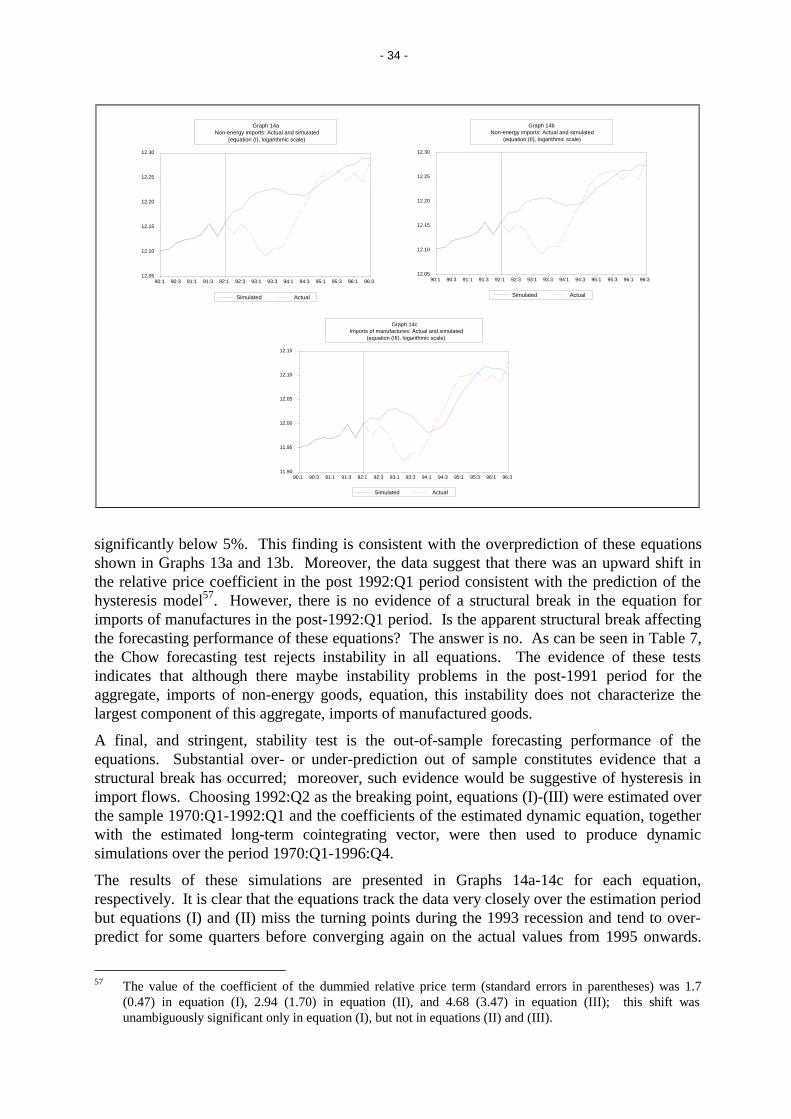
- 34 -

significantly below 5%. This finding is consistent with the overprediction of these equationsshown in Graphs 13a and 13b. Moreover, the data suggest that there was an upward shift inthe relative price coefficient in the post 1992:Q1 period consistent with the prediction of thehysteresis model57. However, there is no evidence of a structural break in the equation forimports of manufactures in the post-1992:Q1 period. Is the apparent structural break affectingthe forecasting performance of these equations? The answer is no. As can be seen in Table 7,the Chow forecasting test rejects instability in all equations. The evidence of these testsindicates that although there maybe instability problems in the post-1991 period for theaggregate, imports of non-energy goods, equation, this instability does not characterize thelargest component of this aggregate, imports of manufactured goods.

A final, and stringent, stability test is the out-of-sample forecasting performance of theequations. Substantial over- or under-prediction out of sample constitutes evidence that astructural break has occurred; moreover, such evidence would be suggestive of hysteresis inimport flows. Choosing 1992:Q2 as the breaking point, equations (I)-(III) were estimated overthe sample 1970:Q1-1992:Q1 and the coefficients of the estimated dynamic equation, togetherwith the estimated long-term cointegrating vector, were then used to produce dynamicsimulations over the period 1970:Q1-1996:Q4.

The results of these simulations are presented in Graphs 14a-14c for each equation,respectively. It is clear that the equations track the data very closely over the estimation periodbut equations (I) and (II) miss the turning points during the 1993 recession and tend to over-predict for some quarters before converging again on the actual values from 1995 onwards.

57 The value of the coefficient of the dummied relative price term (standard errors in parentheses) was 1.7

(0.47) in equation (I), 2.94 (1.70) in equation (II), and 4.68 (3.47) in equation (III); this shift wasunambiguously significant only in equation (I), but not in equations (II) and (III).

12.05

12.10

12.15

12.20

12.25

12.30

90:1 90:3 91:1 91:3 92:1 92:3 93:1 93:3 94:1 94:3 95:1 95:3 96:1 96:3

Simulated Actual

Graph 14aNon-energy imports: Actual and simulated

(equation (I), logarithmic scale)

12.05

12.10

12.15

12.20

12.25

12.30

90:1 90:3 91:1 91:3 92:1 92:3 93:1 93:3 94:1 94:3 95:1 95:3 96:1 96:3

Simulated Actual

Graph 14bNon-energy imports: Actual and simulated

(equation (II), logarithmic scale)

11.90

11.95

12.00

12.05

12.10

12.15

90:1 90:3 91:1 91:3 92:1 92:3 93:1 93:3 94:1 94:3 95:1 95:3 96:1 96:3

Simulated Actual

Graph 14cImports of manufactures: Actual and simulated

(equation (III), logarithmic scale)

- 35 -

However, equation (III), imports of manufactures, reproduces the data very well and shows noevidence of structural break. Since imports of manufactures represent the dominantcomponent of non-energy imports, the apparent modest instability of the non-energy importsequations may be a reflection of instability in the remaining components of the importaggregate. Finally, the evidence from the out-of-sample simulations is consistent with testresults for structural stability reported previously. It is possible to conclude, therefore, thatthere has been no hysteresis phenomena in French imports in recent years, and the simulationssuggest that the flattening out of import growth in the 1990s is likely the result of theslowdown of economic growth.

9,,��'HWHUPLQDQWV�RI�H[SRUWV��6SHFLILFDWLRQ�DQG�HVWLPDWLRQ�UHVXOWV

The estimated equation for the long-run demand for exports, in a specification similar to thatused for imports, has the following parsimonious form:

;W� �α��β <Z��γ 5((5W (16)

where all data are in logarithms, and ;�= volume of export goods, <Z = world demand58 and5((5�= real effective exchange rate (or a relative price term). Equation (16) is assumed torepresent the cointegrating, long-run relationship between exports, world demand and pricecompetitiveness.

The data and mnemonics used in the regression are as follows (all data are in logarithms):(;3121( = non-energy exports; (;304 = exports of manufactures; :''� = worlddomestic demand; (;8/&�� = real exchange rate in terms of relative unit labour costs in totaleconomy against 23 industrial countries; (;*'3�� real exchange rate in terms of relativeGDP deflators against 23 industrial countries; details of data sources are presented in AnnexA.

Three different equations have been estimated on quarterly data over the period 1970:Q1-1996:Q3: equation (IV), where the dependent variable is non-energy exports and the realeffective exchange rate is defined in terms of unit labour costs as a proxy for relative exportprices59; equation (V), where the dependent variable is again non-energy exports but the realeffective exchange rate is defined by relative GDP deflators against the IC-23; and equation(VI) where the dependent variable is exports of manufactures and the real effective exchangerate is defined by relative unit wage costs in manufacturing as a measure of competitiveness60.

58 The world domestic demand (WDD) has been computed as weighted average of the domestic demand in

the following industrial countries: USA, the United Kingdom, Austria, Belgium (GDP), Denmark, Canada,Japan, Germany, Italy, Netherlands , Switzerland, Norway, Finland, Australia, New Zealand, Portugal andSpain. Because of lack of data, the industrialising countries have not been included in the average. Datahave been taken from the WEFA-DRI database, and the main source is the OECD Quarterly NationalAccounts statistics. The weights have been calculated from IMF - Direction of Trade Statistics and arebased on 1970-1995 average of each country's shares in France’s total value of exports of goods.

59 A more appropriate index of relative prices or competitiveness, such as a real effective exchange rate basedon export prices of manufactured goods or of a wider aggregate, is not available. The one calculated by theInternational Monetary Fund covers a more limited period than considered in our analysis. Also, Marquez(1992) shows that, from US trade functions, it is difficult to distinguish empirically between different costand price indicators of international competitiveness.

60 In the Annex E are reported additional cointegration estimates for export equations (IV), (V) and (VI) basedon alternative definitions of competitiveness.

- 36 -

The use of the latter seemsmore appropriate than thatbased on GDP deflators.Real effective exchangerate based on GDPdeflators has been shownto be influenced by twofactors: first, relative unitlabour costs in the tradablesector and, secondly, theratio of unit labour costs intradeables and non-tradeables in eachcountry61. Both definitionsof competitiveness are notaccurately representative ofthe true competitive

position of export goods because they do not capture pricing-to-market behaviour. Not anychange in costs will be automatically and completely passed through to prices of exportedgoods, but also the evolution of unit labour costs and export prices may diverge because ofdifferent product composition of exports and domestic production. Therefore relative unitlabour cost and relative unit wage cost should be considered as ex-ante or underlying,potential, competitive position.

The lag length of the 9(&0 has been set at two, which has proved to be enough to ensureGaussian error terms. In order to decide the most appropriate way of modelling deterministiccomponents in the 9(&0 we have followed the procedure suggested in Johansen (1992b) and,as in the case of imports, based on Pantula principle (starting from the less restrictive model),testing the joint hypothesis of both the rank order and the deterministic components62. Asresult of the procedure, no deterministic variables has entered the cointegration space and the9(&0.

The results of tests on the number of the cointegration vectors are given in Table 8. Thereduced rank test statistics based on trace point to only one cointegrating relationship on theFrench export data. This result greatly simplifies the interpretation of the first vector β1 as along-run equilibrium relationship among export volume, world domestic demand and pricecompetitiveness. The coefficient estimates of the cointegrating relation are reported in theupper panel of Table 8. It is worth noting that the estimated long-run world demand andrelative price elasticities are consistent with those often found in other studies.63

The feedback coefficients in the first column of normalised α’ (reported in Table 9) representthe weights with which excess demand for exports enters the three equations of our system andcan be interpreted as the average speed of adjustment towards the estimated equilibriumrelationship. The first weight, (α1) is referred to the export demand equation and it impliesthat, in the case of model IV, a 1% deviation from equilibrium will be corrected by anadjustment of 0.05. % each quarter. The interesting result, also noted in the case of the import

61 See Marston (1987).62 See Harris (1995).63 For similar results based on cointegration and error-correction methodology see Capet and Gudin de

Vallerin (1993).

Table 8Exports, world demand and relative prices

Johansen likelihood ratio tests for cointegration, trace test

Nocointegration

At mostone vector

At most twovectors

Sample 1970:Q1-1996:Q3

(LJHQYDOXH ��

Non-energy exports, equation (IV) 31.06** 4.08 0.95(LJHQYDOXH ��

Non-energy exports, equation (V) 31.65** 4.98 1.31(LJHQYDOXH ��

Exports of manufactures, equation(VI)

29.89** 3.01 0.75

The null hypotheses are that there is no cointegration, that there is at most onecointegration vector, and that there is at most two cointegration vectors; the 5% criticalvalues of the likelihood ratio statistic at the three largest eigenvalues reported for eachequation in the Table are 24.3, 12.5 and 3.8; the 1% critical values are,correspondingly, 27.9, 16.3 and 6.5; * (**) rejects the null at the 5% (1%) level ofsignificance; equations (IV), (V), and (VI) refer to those in Table 9.

- 37 -

Table 9

Demand for exportsRestricted cointegration/error correction model for exports, world demand, and real effective

exchange rate, 1970:Q1-1996:Q3(equations (IV)-(VI), standard errors in parentheses)

Non-energy exports Exports of manufactures

(IV) (V) (VI)

Cointegrating vector

WDD 1.649 1.719 WDD 1.581(0.154) (0.139) (0.168)

EXULC23 -0.621 EXULC23 -0.552(0.166) (0.181)

EXPGDP23 -0.697(0.149)

ã1 -0.051 (0.012) -0.059 (0.015) ã1 -0.045 (0.012)ã2 -0.018 (0.004) -0.022 (0.005) ã2 -0.018 (0.004)ã3 -0.005 (0.011) -0.006 (0.013) ã3 -0.000 (0.010)

Short-term adjustment model

θ -0.045 -0.050 θ -0.027(0.013) (0.016) (0.012)

d(EXPNONE(-1)) -0.276 -0.239 d(EXPMQ(-1)) -0.269(0.094) (0.093) (0.095)

d(EXPNONE(-2)) -0.169 -0.162(0.091) (0.089)

d(WDD) 0.788 0.828 d(WDD) 1.0170.282) (0.282) (0.298)

d(WDD(-1)) 0.902 0.908 d(WDD(-1)) 0.746(0.303) (0.304) (0.298)

d(EXULC23) -0.139 d(EXULC23(-1)) -0.276(0.104) (0.111)

d(EXULC23(-1)) -0.169 d(EXULC23(-2)) -0.148(0.109) (0.012)

d(EXULC23(-2)) -0.146(0.107)

d(EXPGDP23(-1) -0.260(0.102)

R² 0.268 0.260 R² 0.260SER 0.020 0.020 SER 0.021DW 1.92 2.02 DW 2.00

Jarque-Bera χ² (2) 4.704 2.963 Jarque-Bera χ² (2) 1.666F(ARCH(4)) 0.415 (0.80) 0.295 (0.88) F(ARCH(4)) 0.700 (0.59)F(RESET) 1.200 (0.32) 1.518 (0.19) F(RESET) 1.189 (0.32)F(HET1) 0.972 (0.49) 1.043 (0.42) F(HET1) 1.170 (0.32)F(HET2) 0.799 (0.78) 0.832 (0.70) F(HET2) 0.643 (0.90)F(AR(4)) 0.415 (0.80) 0.191 (0.94) F(AR(4)) 1.455 (0.22)

ãi refers to the value of the adjustment coefficient on the export function entering the first, the second(WDD) and third (relative price) equation, respectively, in the VAR; θ is the error correction term; d(Z)is the first-difference operator for Z; SER is the standard error of the regression; DW is the Durbin-Watson statistic; the Jarque-Bera statistic for the normality of the residuals, distributed as χ² with twodegrees of freedom, has a 95% critical value of 5.99; F(ARCH(4)) of lag order 4 is the F test forautoregressive conditional heteroscedasticity (probability in parentheses); F(RESET) is Ramsey’s Fstatistic for specification error run on five fitted terms; F(HET1) is White’s F test for heteroscedasticity,no cross terms; F(HET2) is White’s F test for heteroscedasticity, with cross terms; F(AR(4)) is the LMtest for serial correlation of order 4; sample 1970:1-1996:4.

- 38 -

3.6

4.0

4.4

4.8

5.2

5.6

70 72 74 76 78 80 82 84 86 88 90 92 94 96

Long-term Actual Simulated

Graph 15aNon-energy exports: Long-term, actual, and simulated

(equation (IV), logarithmic scale)

3.6

4.0

4.4

4.8

5.2

5.6

70 72 74 76 78 80 82 84 86 88 90 92 94 96


Graph 15bNon-energy exports: Long-term, actual, and simulated

(equation (V), logarithmic scale))

3.6

4.0

4.4

4.8

5.2

5.6

70 72 74 76 78 80 82 84 86 88 90 92 94 96


Graph 15cExports of manufactures: Long-term, actual, and simulated

(equation (VI), logarithmic scale)

- 39 -

equation, is that α2 and α3 are virtually negligible, indicating that a disequilibrium in exportdemand induces adjustment only in the first (export demand) equation. As in the importequation, this legitimises the use of a single equation estimation, supporting the assumptionthat world domestic demand and real effective exchange rates are weakly exogenous64 for theparameters in the conditional export demand equation.

The estimated long-run export equations have the following form:

(;3121(� �� :''�� (;8/&�� (17)

(;3121(� �� :''�� (;3*'3�� (18)

(;304� �� :''�� (;8/&�� (19)

The results of the cointegrating equations imply that in the long-run the income elasticity ofexports is quite high (one-percentage point growth in world demand increases manufacturesexports by 1.58% and non-energy products by 1.65%), while the relative price elasticity islower (respectively only -0.55 and -0.62%). The most significant implication of this result, inaccordance with that found in the estimates of import functions, is that changes in France’strade balance will be dominated by real income (domestic demand) movements at home andabroad. The income responsiveness of exports is lower than the income elasticity of importsin all the three equations. This result, although problematic in terms of the external constrainton the rate of growth of economic activity in France, as will be discussed later (see sectionIX), is not surprising and is in accordance with the Houthakker-Magee (1969) asymmetry inthe estimated elasticities found for many industrialised countries. Yet, the high value ofestimated income elasticity may be due to the fact that the scale variable is likely to reflectalso the impact of other non-price effects, such as product diversification, quality differencesand above all supply-side effects. Furthermore, the high income elasticity may be also due tosome upward bias reflecting the effect of tariff reductions and other trade liberalisationpolicies, which is difficult to estimate separately because of the lack of data.

In order to test the robustness of these findings with respect to the choice of the relative priceterm we have re-estimated the long-run relationship using different competitiveness measures.The results of the Johansen cointegration analysis, reported separately in Annex E, Table E1,turned out to be very similar to those reported in Table 9.

In the next step of the analysis, the estimated cointegrating vector was embedded in a dynamicerror-correction model which was estimated by OLS. Its specification follows closely that ofthe imports equations (see equation (12) and the discussion in sections IV and V). Initially,four lags of the first-differenced variables were used, which provided a sufficientrepresentation of the process generating the quarterly time series. Then, following a general-to-specific simplification procedure, we have eliminated negligible and insignificant effectsthrough a sequential reduction. The final restricted conditional model resulting from thesimplification procedure are reported in the lower panel of Table 965. All regressioncoefficients show the expected signs and the diagnostic test statistics are quite satisfactory.The three models track the size and the direction of changes in the volume of non-energy andmanufactured exports fairly well (see Graphs 15a-15c).

64 See comment in footnote 46 on the exogeneity status of variables.65 Following the approach suggested by Hendry we have taken into account statistics associated with the

implied reductions, that is F statistic, Schwarz criterion and standard error of regression.

- 40 -

The parameter estimate on the error-correction term, that reflects the impact on ∆[ of having[W�� out of the long-run equilibrium condition, has the right sign (which must be negative forthe purpose of dynamic stability and cointegration) and appears significant at 5% level.Therefore, the deviation from the equilibrium due to random shocks represents a significantdeterminant of the export short-run dynamic behaviour. The estimates show a very slowadjustment to disequilibrium (3% each quarter for the export of manufactures and 4.5% forthe non-energy exports equation when relative unit labour costs is used) which can arise fromshocks in determinants of export demand, revealing the presence of large adjustment costs(such as transaction costs, search costs and costs linked to modifying capacity utilisation etc.)or other factors such as contract lags or order-delivery lags.

The estimates of the three equations satisfy all of the diagnostic statistics at their 95% criticalvalue, so the models have approximately white noise, homoschedastic, normally distributedresiduals, which can be considered innovations with respect to the current and laggedvariables in the regressions. None of the regression coefficients displays any evidence ofinstability66. Therefore, the estimated models seem general enough to capture all the salientfeatures of, and to provide an adequate representation of the process generating, the data;thus, it is possible to conclude that three satisfactory models for non-energy andmanufacturing good exports have been achieved.

In view of the fact that the dynamic equations explain the rate of changes in the exportvariables, the adjusted R2 value can be considered quite good (0.27 for equation IV and 0.26for equations V and VI). The estimated standard errors (around 0.020) are also small. Takinginto account the substantial fluctuations in the sample period, in particular those related to thetwo oil crises, the models explain the changes in export demand rather accurately (see also theplots of actual and fitted values in Graphs 15a-15c).

The evidence in Table 9 shows that both the short-run income and price elasticities are smallerthan the long-run elasticities. The size of the coefficients shows large and immediate effect ofa change in world demand on export demand for France’s commodities (the impact elasticity,that is the response in the current quarter is around 0,80 ), but a smaller, and one- or even two-quarter lagged, impact of a change in competitiveness is suggested by the estimates. This is acommon result in trade flows analysis where the data show that activity lags are much shorterthan price or competitiveness lags.

The timing of adjustment and the size of the export price elasticity are both important forissues of exchange rate adjustments. The results of our estimate show that competitivenesshas a predictable and systematic impact on export flows, but the elasticity is found to be lowand below unity. A depreciation of 10 per cent, if completely passed-through into exportprices, in our model will cause a reduction of almost 5 per cent in manufactures and non-energy export volumes but the reduction will take effect only after a quarter or two.

9,,,��+\VWHUHVLV�LQ�H[SRUWV�DQG�VWDELOLW\�RI�WKH�HVWLPDWHV

To investigate the issue of parameter constancy of our export models we turn now to results ofrecursive estimation. Structural instabilities may be interpreted as signalling hysteresisphenomena; in the event of competitiveness shocks, such as the real appreciation of theFrench franc through the first half 1990s, it is possible that this may have had adverse effects

66 Parameter instability statistics are based on the recent procedure suggested by Hansen (1992), which is

aimed to test the stability of each parameter individually and the stability of all the parameters jointly;results of these tests are available upon request.

- 41 -

on export performance67. In particular, theappreciation of the real exchange rate forthe French franc may have contributed topricing French exporters out of theinternational markets where Frenchproducts are imperfectly substitutable withother goods, and this is especially the casefor exports of manufactures. On the otherhand, it is possible that improved non-pricecompetitiveness may have boosted exportsabove traditional trends and also above thelevel predicted by the economicallyrelevant determinants.

As in the case of the import functions, wehave first examined the stability of long-term relationship, but unlike the testsreported in section VI, we have chosen hereto run a recursive ),0/ estimate of the9(&0 instead. The Graphs shown in

Annex F plot the recursive eigenvalues associate with each eigenvector. These plotscorrespond to the standard graphs of recursive parameter estimates in the usual models, sincenon-constancy of the weighting elements α and/or in the elements of matrix β would bereflected in the non-constancy of the eigenvalues68. For the three long-term export modelsthere is no evidence of parameter instability due to failure to account for structural breaks.Thus, the estimated cointegration vectors appear to be temporally stable.

Regarding the stability of the dynamic error-correction model, the Graphs in Annex G showthe result of the CUSUM and CUSUM of square tests; again, as in the case of imports, thereis no evidence of structural instabilities in the dynamic equations.

Further insights on the presence of instability in the equations are provided by graphs inAnnex H which plot the values of the recursively estimated coefficients of the dynamic modelalong with their (±2) standard errors, which provide an approximate 95% confidence interval.The intention here is to uncover evidence for instability with reference to the particularparameters of the equations. Again, all coefficients appear to remain inside the ex-antestandard errors for the entire period and vary little, confirming the structural stability of eachof the three models.

As a further test for the presence of structural breaks, possibly arising from the realappreciation of the French franc since the beginning of 1992, we have used Chow test forpredictive failure and Hendry’s forecasting test; we implemented the test, as in the case ofimports, by re-estimating the model up to 1992:Q1 and making one-step forecasts for theperiod ahead. Once again, there is no evidence of parameter instability (see the test statisticsin Table 10). This is in contrast to the findings in the case of imports, where there appears tohave been some instability problems, associated presumably with the competitiveness shockbeginning in 1992:Q1 especially in the case of non-energy imports, equations (I) and (II) - seeTable 7.

67 See Amano et. al. (1993) for a similar investigation of hysteresis in Canadian trade flows in response to the

Canadian dollar’s appreciation.68 See Harris (1995), p. 91.

Table 10

Stability of export equations: Tests for structural break in1992:Q2

(complete sample 1970:Q1-1996:Q4)

F Prob LR (χ²) Prob

1RQ�HQHUJ\�H[SRUWV��(TXDWLRQ��,9�



1RQ�HQHUJ\�H[SRUWV��(TXDWLRQ��9�



([SRUWV�RI�PDQXIDFWXUHV��(TXDWLRQ��9,�



Prob is the probability of drawing an F or a χ² statistic of thevalue shown in the Table from the respective distribution; thenull hypothesis is that there in no structural break, andprobability values of 5% or less can be taken to indicaterejection of the null.

- 42 -

A final test of the stability of the estimated dynamic models was performed in terms of theout-of-sample predictive power of the equations. As in the case of imports, the equationswere estimated up to 1992:Q1 and the coefficients so obtained were used to forecast out to1996:Q3. The quarterly predictive performance is each equation is shown in Graphs 16a-16c.The equations forecast generally well, and clearly better than the companion import equations- compare with results of the present Graphs with those presented in Graphs 14a-14c. Thethree equations tend to over-predict exports in the 1993 recession but, overall, the results arevery good since the deviations from actual are notably modest, especially considering thesharp movements in export volumes during this period. Thus, the evidence from the stabilitytests confirms that the estimated export functions are temporally stable.

,;��)UDQFH¶V�H[WHUQDO�FRQVWUDLQW�DQG�HFRQRPLF�JURZWK

The estimated long-run price and income elasticities of France’s trade flows allow acalculation of the severity of the external balance constraint on domestic policy choices and,more specifically, on the growth rate of domestic demand. Although France does not have atarget for its external accounts, the underlying demand and competitiveness elasticities oftrade flows impose constraints on demand growth given the state of the external accounts.Given these elasticities, demand or competitiveness shocks can explain movements in theexternal accounts such as the surplus of the 1990s. In particular, the external surplus willdecline (increase), ceteris paribus, if domestic demand grows faster (slower) than foreigndemand; alternatively, competitiveness elasticities, or the Marshall-Lerner condition, willdetermine, ceteris paribus, whether the nominal trade surplus will decline as a result of theexchange appreciation of the 1990s. Presently, the stylised model, first proposed by Johnson

4.95

5.00

5.05

5.10

5.15

5.20

5.25

5.30

90:1 90:3 91:1 91:3 92:1 92:3 93:1 93:3 94:1 94:3 95:1 95:3 96:1 96:3

Simulated Actual

Graph 16aNon-energy exports: Actual and simulated

(equation (IV), logarithmic scale)

4.95

5.00

5.05

5.10

5.15

5.20

5.25

5.30

90:1 90:3 91:1 91:3 92:1 92:3 93:1 93:3 94:1 94:3 95:1 95:3 96:1 96:3

Simulated Actual

Graph 16bNon-energy exports: Actual and simulated

(equation (V), logarithlic scale)

4.9

5.0

5.1

5.2

5.3

90:1 90:3 91:1 91:3 92:1 92:3 93:1 93:3 94:1 94:3 95:1 95:3 96:1 96:3

Simulated Actual

Graph 16cExports of manufactures: Actual and simulated

(equation (VI), logarithmic scale)

- 43 -

(1958) and subsequently used widely in the literature69 is the vehicle through which theanalysis is prepared.

The standard foreign trade demand functions, on which we have carried out econometricestimates, can be expressed as follows:

;� �<Zη[�\��3L�H3 �

η[�S (20)

0� �<ηP�\��H3 �3L�ηP�S (21)

where ; = volume of exports, 0 = volume of imports, <Z�= world demand, < = domesticdemand, 3L�= export or domestic prices, 3 = foreign prices in foreign currencies, H = nominalexchange rate, η[�\ = (foreign) demand elasticity of exports, η[�S = relative-price elasticity ofexports (absolute value),�ηP�\ = income elasticity of imports, ηP�S = relative-price elasticity ofimports (absolute value) and 3Z� �H3 = foreign prices in domestic currency.

In terms of rate of change (;¶�and 0¶), equations (20) and (21) can be written as follows:

;µ� �η[�\��<¶Z��η[�S��3¶L��η[�S�3¶�Z(22)

0¶� �ηP�\��<¶��ηP�S��3¶L��ηP�S�3¶�Z (23)

The trade balance in nominal terms is:

�9[��9P�� 3L� �;��3Z� �0 (24)

where 9[ = value of exports and 9P�= value of imports.

Differentiating equation (24) with respect to time, and noting this as G� �δI�δW, we obtain:

G�9[��9P�� ;G3L��3LG;��0G3Z��3ZG0� (25)

where, using the definitions ;� �9[�3L and 0� �9P�3Z and expressing the right hand in termsof rates of change, yields:

G�9[��9P�� 9[��3¶L��;¶��9P�3¶Z��0¶� (26)

Substituting from (23) and (24) we have:

G�9[��9P�� 9[�3¶L��η[�\�<¶Z��η[�S�3¶L��η[�S�3¶�Z��9P�3¶Z��ηP�\�<¶��ηP�S�3¶L�ηP�S3¶Z�� 9[��3¶L��η[�S��η[�S�3¶�Z��η[�\�<¶Z��9P�ηP�S��3¶L��ηP�S�3¶�Z��ηP�\<� (27)

69 See Thirlwall (1978), Rollet (1983), Carone (1995) and Castaldo, Palmisani and Rossi (1986) from which

material for this section has been drawn.

- 44 -

Imposing the invariance of trade balance condition, d(Vx - Vm) = 0, we can solve the (27) forthe rate of growth of domestic demand which is consistent with such invariance :

<¶� ��9[�9P�� η[�\�ηP�\� <¶Z��3µL� ��9[�9P�� η[�S��ηP�S�� ηP�\

��3¶Z� ��ηP�S��9[�9P�� η[�S�� ηP�\ (28)

On the assumption that trade balance is initially in equilibrium, (28) can be rewritten as:

<µ� ��η[�\�ηP�\�� <¶Z��3¶Z��3¶L�� ηP�S��η[�S�� ηP�\ (29)

Equations (28) and (29) are the basic analytical formulations of the external constraint, andshow the critical parameters which, given the evolution of world demand and of relativeprices or competitiveness, determine the rate of growth of domestic activity compatible withthe initial external imbalances (equation (28)), or with equilibrium in the external accounts(equation (29)). Correspondingly, for any rate of growth of domestic demand and evolution ofworld demand, these equations can be solved for the size of the change in competitiveness(that is in the nominal exchange rate or in relative costs or prices) which would be necessaryto achieve a given trade balance position. Finally, the equations summarize succinctly thefactors that impinge on external performance, and ultimately permit us to decompose the tradesurplus according to the contributing factors.

On the assumption of unchanged competitiveness �3¶L� � 3¶Z�, equation (28), in which thetrade balance is in disequilibrium, becomes:

<¶� �<¶Z��η[�\�ηP�\�� 9[�9P��3¶L� ��9[�9P��9P� ��ηP�\ (30)

while equation (30), where the trade balance is assumed to be in equilibrium �9[�9P� ��,becomes:

<µ� ��η[�\�ηP�\�� <¶Z (31)or

<¶�<¶Z� �η[�\�ηP�\ (32)

It is clear that, ceteris paribus, the external constraint is less binding on domestic economicgrowth, the higher is the ratio of income elasticities of exports and imports, �η[�\�ηP�\��moreover, in the case of equations (28) and (30) where 9[�≠�9P��the external constraint is lessbinding the higher is the export/import ratio, 9[�9P.

Measured values of the critical parameters, based on estimates reported in Tables B1 and E1of the Annexes (see the explanatory note in Table 11) are presented in Table 11. The ratio ofexport and import elasticities with respect to income is the dynamic Harrod foreign trademultiplier. In the case of France, and on the basis of our estimates, this ratio shows that thetrade balance (both for manufactures and for non-energy products) would act as a constrainton income or domestic demand growth since had it been greater than world demand growththe external surplus (deficit) would be smaller (larger), as can be seen from η[�\�ηP�\�<��. Onthe assumption of constant competitiveness and initially unbalanced trade, it is clear that,using the values of imports and exports in 1995, the maximum rate of growth of domesticdemand in 1995 which would have permitted to sustain a given trade balance position was

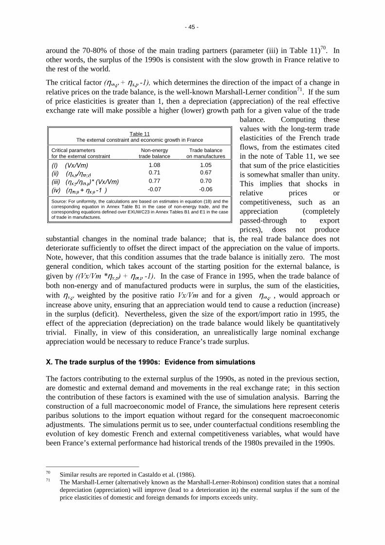
- 45 -

around the 70-80% of those of the main trading partners (parameter (iii) in Table 11)70. Inother words, the surplus of the 1990s is consistent with the slow growth in France relative tothe rest of the world.

The critical factor��ηP�S��η[�S�� which determines the direction of the impact of a change inrelative prices on the trade balance, is the well-known Marshall-Lerner condition71. If the sumof price elasticities is greater than 1, then a depreciation (appreciation) of the real effectiveexchange rate will make possible a higher (lower) growth path for a given value of the trade

balance. Computing thesevalues with the long-term tradeelasticities of the French tradeflows, from the estimates citedin the note of Table 11, we seethat sum of the price elasticitiesis somewhat smaller than unity.This implies that shocks inrelative prices orcompetitiveness, such as anappreciation (completelypassed-through to exportprices), does not produce

substantial changes in the nominal trade balance; that is, the real trade balance does notdeteriorate sufficiently to offset the direct impact of the appreciation on the value of imports.Note, however, that this condition assumes that the trade balance is initially zero. The mostgeneral condition, which takes account of the starting position for the external balance, isgiven by ��9[�9P� η[�S��ηP�S��. In the case of France in 1995, when the trade balance ofboth non-energy and of manufactured products were in surplus, the sum of the elasticities,with η[�S weighted by the positive ratio 9[�9P and for a given �ηP�S� , would approach orincrease above unity, ensuring that an appreciation would tend to cause a reduction (increase)in the surplus (deficit). Nevertheless, given the size of the export/import ratio in 1995, theeffect of the appreciation (depreciation) on the trade balance would likely be quantitativelytrivial. Finally, in view of this consideration, an unrealistically large nominal exchangeappreciation would be necessary to reduce France’s trade surplus.

;��7KH�WUDGH�VXUSOXV�RI�WKH��V��(YLGHQFH�IURP�VLPXODWLRQV

The factors contributing to the external surplus of the 1990s, as noted in the previous section,are domestic and external demand and movements in the real exchange rate; in this sectionthe contribution of these factors is examined with the use of simulation analysis. Barring theconstruction of a full macroeconomic model of France, the simulations here represent ceterisparibus solutions to the import equation without regard for the consequent macroeconomicadjustments. The simulations permit us to see, under counterfactual conditions resembling theevolution of key domestic French and external competitiveness variables, what would havebeen France’s external performance had historical trends of the 1980s prevailed in the 1990s.

70 Similar results are reported in Castaldo et al. (1986).71 The Marshall-Lerner (alternatively known as the Marshall-Lerner-Robinson) condition states that a nominal

depreciation (appreciation) will improve (lead to a deterioration in) the external surplus if the sum of theprice elasticities of domestic and foreign demands for imports exceeds unity.

Table 11The external constraint and economic growth in France

Critical parametersfor the external constraint

Non-energytrade balance

Trade balanceon manufactures

�,��9[�9P� 1.08 1.05

�LL��η[�\�ηP�\�0.71 0.67

�LLL��η[�\�ηP�\� ��9[�9P� 0.77 0.70

�LY��ηP�S��η[�S�� -0.07 -0.06

Source: For uniformity, the calculations are based on estimates in equation (18) and thecorresponding equation in Annex Table B1 in the case of non-energy trade, and thecorresponding equations defined over EXUWC23 in Annex Tables B1 and E1 in the caseof trade in manufactures.

- 46 -

A representative import equation estimatedpreviously is used to conduct thesimulations. Since there is no evidence ofinstability in the export functions, itconfirms that the source of the surpluscannot have been the superior exportperformance, because actual exports haveevolved according to the prediction of theequations. It is, rather, that in the importside of the accounts that the source of thesurplus can be found. Consequently, thesimulations have been based on an estimatedrepresentative import equation.

Graph 12 and the discussion in sections V,VII and IX have suggested that the slowgrowth of domestic demand in France haslikely been an important factor in theexternal surplus. One way to evaluate this isto assume that demand growth in France inthe 1990s has followed the same trend as inthe second half of the 1980s and, consistentwith the evidence from the stability tests,that there is no break in the relationshipbetween imports and domestic demand.Fitting a trend on domestic demand over theperiod 1985:Q1-1990:Q4 yields thefollowing equation: DDO2 = 1077.899 +31.35197*Time; this equation was used to

forecast domestic demand over the period 1991:Q1-1996:Q4, and the latter variable was usedto simulate the demand for imports over this period. Correspondingly, actual data formovements in the franc real exchange rate in the period 1990:Q1-1996:Q4 was used toconstruct the real exchange rate shock. Using as a representative demand for imports equation(I), demand for non-energy imports, the results shown in Graphs 17a and 17b are obtained. InGraph 17a the (logarithmic) level of non-energy imports in 1980 prices is presented, whileGraph 17b shows the deviation of imports from their actual value as percent of actualaccording to each shock.

As can be seen in Graphs 17a and 17b, the appreciation of the franc real exchange rate has,ceteris paribus, contributed to raising the demand for non-energy imports by as much as 13%at its peak in 1993:Q2. However, during the overall period the impact of the appreciation hasbeen modest; after 1993 import demand returns to its actual level and the impact of the realexchange rate shocks fades away, as can be seen from the convergence of actual and simulatedimports under this shock.

Substantially more pronounced is the impact of the domestic demand shock. Had domesticdemand followed the growth path of the second half of the 1980s, imports would haveincreased markedly in the 1990s, especially during the slow growth and the recession quartersof 1992 and 1993, as can be seen from Graph 17a. The recovery of domestic demand growthin 1994 and 1995, by bringing domestic demand closer to its trend value of the second half ofthe 1980s, contributed towards reducing the deviation between the simulated and actual

Graph 17aThe impact of the real exchange rate and of domestic demand

on non-energy imports(simulation results, equation (I), logarithmic scale)

11.4

11.6

11.8

12.0

12.2

12.4

12.6

12.8

80 81 82 83 84 85 86 87 88 89 90 91 92 93 94 95 96

Real exchange rate Domestic demand Actual imports

Graph 17bThe impact of the real exchange rate and of domestic demand

on non-energy imports(shock minus actual as percent of actual)

-10

0

10

20

30

40

50

90:1 90:3 91:1 91:3 92:1 92:3 93:1 93:3 94:1 94:3 95:1 95:3 96:1 96:3

Exchange rate shock Domestic demand shock

- 47 -

imports during this period. The results of this simulation show conclusively that a principalfactor in the external surplus of the 1990s can be found in the import side of the accounts,where the recession and slow growth of domestic demand have depressed imports. As can beseen from Graph 17b, the volume of non-energy imports in this counterfactual would havebeen on average over 30% higher than actual in the post-1993 period thus, ceteris paribus, notonly eliminating completely the external surplus but in fact causing the accounts to move intodeficit.

;,��&RQFOXGLQJ�UHPDUNV

France’s external performance since the beginning of the 1990s has been remarkable, with themerchandise trade and the current account balance rising to over 1.5% of GDP in 1996. Thesedevelopments have taken place against a loss of price and cost competitiveness, and in thecontext of slow growth in France relative to its major partners. It has been argued that theexternal surpluses are indicative of changing fortunes, characterized by improving tradeperformance symptomatic of structural changes in import and export equations. Closerreview of the data suggests that since 1990 the relatively larger rise in export than in importvolumes dominates the contribution of the terms of trade in movements in both the non-energy trade balance and in the balance on manufactures.

In the paper, the behavioural content of the trade flow adjustments in response tocompetitiveness and output shocks was developed in a cointegration/error-correctionframework. This framework permits the determination of the long-term equilibriumrelationship between imports, and exports, and their economic determinants while, at the sametime, it allows the characterization of adjustment towards equilibrium when deviations ofpredicted from actual trade flows emerge. This characterization is important since trade flowsrespond to shocks with variable lags and with varying weights. The results obtained in thesample of quarterly data starting in the beginning of the 1970s to the end of 1996 show thatthe coefficient adjustment in question is very large in the case of imports (where deviationsfrom equilibrium are virtually eliminated with a year) but substantially slower in the case ofexports. This implies that movements in the external accounts in response to shocks reflectpredominantly adjustments in the import side of the accounts.

Both the cointegration relationship and the dynamic adjustment part of the estimatedeconometric models for imports, and for exports, of non-energy products and formanufactures appear to be temporally stable. However, there is some qualified evidence ofinstability in some specifications of the import equations. This instability, which appears tobe temporary and does not affect the forecasting performance of the import equations, is likelyrelated to a temporary break in the competitiveness elasticity in the beginning of 1992 whenthe large real appreciation of the French franc commenced. While instability is hinted at inthe import equation for non-energy products, there is no evidence of instability in the case ofthe largest component of France’s imports, imports of manufactures. In view of the broadstability of the import functions, and together with the absence of evidence of instability in theexport functions, it is possible to reject the hypothesis that part of the surplus of the 1990s isin any way due to better performance in trade unrelated to historical relationships. Thestability tests also provide some preliminary, but not conclusive, evidence against thehypothesis of hysteresis in French trade flows as a result of the competitiveness shocks of the1990s.

The econometric results confirm that, consistent with earlier empirical work, the long-rundemand elasticity of imports and of exports is substantially higher than the competitiveness

- 48 -

elasticity. By implication, the demand shocks associated with the recession and slow growthof the first half of the 1990s have played a dominant role in the growth of imports below thepath observed during the high growth period of the second half of the 1980s. Simulationsshow that the dominant part of the surplus of the 1990s can be attributed immediately to thelower growth trajectory of domestic demand in France compared to its path in the second halfof the 1980s which has led to a decline in the volume of imports below their trajectory overthe second half of the 1980s. It is clear that, should recovery of growth at historical rates beachieved in coming quarters, the external accounts will undoubtedly see the disappearance ofthe surplus.

The importance of economic growth in determining movements in France’s external accountsin the 1990s can also be evaluated from the perspective of how binding the external constraintfor economic growth is. In particular, given the estimated trade flow elasticities with respectto demand and to competitiveness and given world demand growth, a given trade balance canbe solved either for the implicit domestic demand growth consistent with this configuration;or for the level of competitiveness consistent with a given trade balance. The empiricalestimates suggest that, not surprisingly, the external surplus is consistent with the slowdownon economic growth in France relative to her trading partners in the 1990s. Indeed, theestimates suggest that the good trade performance is consistent with demand growth in Francein the range of 70% to 80% of demand growth abroad.

Much concern has been raised by the ERM turbulence of 1992 and 1993 in its potentialadverse implications of the depreciations of several currencies for France’s price and costcompetitiveness, but the results obtained here do not support these concerns. France’s tradeflows are elastic with respect to competitiveness shocks although these elasticities are dwarfedby the demand elasticities. The estimates also suggest that there is a significant quantitativedifference between the competitiveness elasticity of exports compared to that of imports, withthe former being two to three times as large as the latter. However, for the trade balance, it isthe sum of the competitiveness elasticities that matter, and the estimates suggest that theMarshall-Lerner condition in the sample under review is just met. Consequently, the evidencedoes not lend to this issue, which so exercized the French authorities in the aftermath of theERM exchange rate crises of the early 1990s; however, although these shocks do not impingesignificantly on the trade balance, they will have significantly more impact on the export-oriented sector of the economy.

A fundamental change in EMU will be that nominal exchange rate adjustments will not beavailable to affect temporarily competitiveness. Consequently, sustaining goodcompetitiveness trends would require that, among others, favourable cost trends, or policies ofcompetitive disinflation, continue to prevail. There are undoubtedly limits to such policiesand, in an environment of low inflation and disciplined cost developments, such limits may berapidly reached. At the same time, it is likely that the synchronization of business cyclesacross the EU Member States will be reinforced through policy co-ordination, with the resultthat France’s demand-determined external account movements and the frequency of externalimbalances would tend to be reduced. In these circumstances, sustaining a good tradeperformance would require principally policies enhancing modernization and innovation ofthe enterprise sector as well as improvements in the quality of factor inputs in the competitivesector of the economy.

- 49 -

$11(;�$

6RXUFHV�DQG�7LPH�6HULHV�3URSHUWLHV�RI�WKH�'DWD

The principal source of the data is the INSEE databank 6pULHV�7ULPHVWULHOOHV�GH�&RPSWDELOLWp1DWLRQDOH� GH� O¶,16(( and all constant-price variables are 1980 prices. Real exchange ratevariables, also indexed at 1980=100, have been prepared in DG-II, Directorate D. Othervariables, denoted as calculated in Table A1, have been defined as combinations of theoriginal variables.

As noted in the text, it is essential that in order to obtain meaningful statistical results the timeseries used in the empirical work are stationary. Results of stationarity tests are presented inTable A1. All data are in logarithms. The equation used in the testing procedure was definedover an intercept alone; identical results were also obtained from an equation including a time

trend. For the majority of the data the null of nonstationarity cannot be rejected in level format either the 99% of the 95% level of significance. Correspondingly, the null of stationarity isoverwhelmingly accepted when the data is first differenced; thus such variables are integratedof order one �,��. One exception to this is the data for real exchange rate defined in terms ofrelative unit wage costs in manufacturing against the IC-23 and the IC-20. For these

Table A1Sources and time-series properties (stationarity tests) of the data

(Sample 1970:Q1-1996:Q4, except prices 1970:Q1-1996:Q3)

Level First difference

Variable Source DF ADF(4) DF ADF(4) ~I(z)

Domestic demand PDI_V008 -1.90 -2.48 -8.25 -4.67 I(1)

Non-energy imports P60_V008-P60_U038 -1.74 -1.82 -8.68 -5.83 I(1)

Imports of manufactures P60_V098 -1.66 -1.76 -9.68 -6.37 I(1)

Import price/GDP deflator Calculated -0.25 -0.09 -6.78 -5.65 I(1)

Import price/domestic demand deflator Calculated -0.27 -0.17 -6.59 -5.86 I(1)

Manufactures, import/domestic price Calculated -0.97 -0.86 -8.91 -5.51 I(1)

Non-energy exports P50_V0M8-P50_U038 -1.98 -1.88 -10.40 -4.35 I(1)

Exports of manufactures P50_V098 -1.96 -1.69 -10.40 -4.66 I(1)

World domestic demand Calculated 0.02 -0.19 -8.58 -3.98 I(1)

Real exchange rate IC-23, GDP deflators Commission services -2.22 -2.46 -7.56 -4.69 I(1)

Real exchange rate IC-20, GDP deflators Commission services -2.17 -2.37 -7.61 -4.66 I(1)

Real exchange rate EU-14, GDP deflators Commission services -2.49 -2.41 -8.75 -5.04 I(1)

Real exchange rate IC-23, unit labour costs Commission services -2.03 -2.11 -7.51 -4.82 I(1)

Real exchange rate IC-20, unit labour costs Commission services -1.97 -2.03 -7.56 -4.77 I(1)

Real exchange rate EU-14, unit labour costs Commission services -2.02 -1.98 -8.49 -4.76 I(1)

Real exchange rate IC-23, unit wage costs Commission services -2.66 -3.37 -7.49 -4.73 I(0)

Real exchange rate IC-20, unit wage costs Commission services -2.61 -3.28 -7.68 -4.69 I(0)

Real exchange rate EU-14, unit wage costs Commission services -2.58 -2.74 -8.59 -4.74 I(1)

DF and ADF statistics are the Dickey-Fuller and the augmented Dickey-Fuller statistics, respectively; ADF (4) isthe ADF statistic of order 4; the critical value of the DF and the ADF statistics, calculated by the MacKinnonmethod, at the 99% level of significance, is -3.50, and at the 95% level of significance it is -2.89; the teststatistics are obtained from an equation defined over an intercept; ~I(z) signifies that the order of integration is z;all constant-price variables are defined in 1980 prices.

The principal source of the data is the INSEE databank 6pULHV� 7ULPHVWULHOOHV� GH�&RPSWDELOLWp� 1DWLRQDOH� GH� O¶,16((, and each variable corresponds to the INSEE databank mnemonic indicated in the table; calculatedvalues are from the original data; the world demand series was prepared at ISCO; the source of the remainingdata is the Commission services and all measures of the real exchange rate have been prepared in DG-II,Directorate D-4.

- 50 -

variables, only the ')�statistics reject the null of stationarity in level form and these seriesappear to be ,�� however, the $')�� statistics suggest that these series are ,��. Finally,virtually all other variables are ,�� either by the ') or by the $')�� statistic, as can be seenfrom the results reported in the third and fourth columns of the Table.

- 51 -

$11(;�%

)XUWKHU�&RLQWHJUDWLRQ�5HVXOWV��,PSRUW�(TXDWLRQV��,��,,,�

This annex presents additional FIML cointegration estimates for import equations (I)-(III)based on alternative definitions of competitiveness. The estimation results reported insections V and VI were based on the price of imports relative to the relevant domesticdemand deflator, a strategy intended to capture pricing-to-market behaviour and similarphenomena. According to this view, competitiveness approximated by conventional realexchange rate variables would not be accurately representative of the true competitiveposition of exports and importers. However, competitiveness defined by real exchange ratesand by relative costs are important concept in themselves, widely used in empirical tradefunctions, and their role deserves investigation in quantitative import functions.

A review of the empirical importance of real exchange rate variables for French imports wasundertaken over the sample 1970:Q1 - 1996:Q4, and the results are presented in Table B1.The equations are cointegration vectors for non-energy imports and imports of manufacturesand domestic demand and the real exchange rate. In the first panel of the Table, referring tonon-energy imports, the real exchange rate variable is defined by the double export-weightedvalue of an index in terms of the relative GDP deflators; the second panel, also referring tonon-energy imports, shows the same cointegration results for the real exchange rate definedin terms of the relative unit labour costs in total economy; and the third panel presentscointegration results for imports of manufactures where the real exchange rate term isdefined by the relative unit wage costs in manufacturing. Three sets of results are reported ineach panel: first, results for the real exchange rate against the IC-23; secondly, results forthe real exchange rate against the IC-20; and, third, results for the real exchange rate againstthe 14 EU Member States. For each equation the relevant cointegration vector is also writtenout. The mnemonics used in the Table are as follows (all variables in logarithms):

,03121( = non-energy imports; ''2� = domestic demand including stocks; (;3*'3M= real exchange rate in terms of relative GDP deflators, j indexes the country group againstwhich the real exchange rate is measured, = 23, 20, 14; (;8/&M = real exchange rate interms of relative unit labour costs in total economy, j = 23, 20, 14; ,0304 = imports ofmanufactures; and (;8:&M = real exchange rate in terms of relative unit wage costs inmanufacturing, j = 23, 20, 14. All variables are in 1980 prices and the real exchange rateindices have a value of 100 in 1980. The statistical properties of the variables used arereported in the previous Annex, Table A1.

In the first panel, the result do not reject cointegration between non-energy imports, domesticdemand and the real exchange rate at the 95% level of significance, and at the largesteigenvalue the vector is unique. The long-term import equation has an identical domesticdemand and real exchange rate elasticity (2.4 and 0.2, respectively) irrespective of whetherthe real exchange rate is defined in terms of the IC-23 or the IC-20 industrial group. In thecase of imports of manufactures, however, the vector is determined at the 99% level ofsignificance and, while the domestic demand elasticity is not different from its valueestimated in the previous two equations, the real exchange rate elasticity against the EU-14,at 0.5, is more than twice as high as that reported in the previous equations.

- 52 -

Table B1Imports, domestic demand and the real exchange rate

Johansen likelihood ratio tests for cointegration(sample 1970:Q1 - 1996:Q4)

Nocointegration

At most onevector

At most twovectors

(LJHQYDOXH ��

Non-energy imports, equation (I) 30.22* 12.13 4.05*

Cointegrating vector: IMPNONE = 22.12 + 2.42*DDO2 + 0.23*EXPGDP23

(LJHQYDOXH 0.157 0.074 0.037

Non-energy imports, equation (I) 29.91* 12.04 4.01*


(LJHQYDOXH ��

Non-energy imports, equation (I) 37.88** 13.78 4.53*


(LJHQYDOXH ��

Non-energy imports, equation (II) 31.60* 11.21 4.08*

Cointegrating vector: IMPNONE = 22.01 + 2.45*DDO2 + 0.27*EXULC23

(LJHQYDOXH ��

Non-energy imports, equation (II) 31.08* 10.88 4.14*


(LJHQYDOXH ��

Non-energy imports, equation (II) 30.89* 11.07 3.72


(LJHQYDOXH ��

Imports of manufactures, equation (III) 40.17** 15.56* 4.03*

Cointegrating vector: IMPMQ = 23.77 + 2.51*DDO2 + 0.29*EXUWC23

(LJHQYDOXH ��

Imports of manufactures, equation (III) 39.80** 15.43* 3.96*


(LJHQYDOXH ��

Imports of manufactures, equation (III) 37.90** 12.96 4.70*


The null hypotheses are that there is no cointegration, that there is at most one cointegration vector,and that there is at most two cointegration vectors; the 5% critical values of the likelihood ratio statisticat the three largest eigenvalues reported for each equation in the Table are 29.68, 15.41 and 3.76; the1% critical values are, correspondingly, 35.65, 20.04 and 6.65; * (**) rejects the null at the 5% (1%)level of significance; equations (I), (II), and (III) refer to those in Table 5 of the main text.

- 53 -

These estimates appear to suggest that price competitiveness in manufacturing against theEU-14 group is quantitatively more important than compared to the other trading groupsbecause intra-EU real exchange rate shocks influence imports of manufactures significantlymore than other competitiveness shocks.

The results reported in the second panel suggest that while cointegration is generallysupported by the data, this occurs at only the 95% level of significance; no vector issignificant at a more stringent level. Thus, the definition of cost competitiveness by therelative unit labour costs in the total economy finds somewhat weaker support in the long-term import equations. Nevertheless, at this level of significance, the estimated domesticdemand elasticity of imports is virtually identical in the three equations. Moreover, theelasticity of imports with respect to the real exchange rate is identical in the three equations.

The third panel of the Table presents results for imports of manufactures with the costcompetitiveness term approximated by relative unit wage costs in manufacturing. In allequations the presence of cointegration is supported at the 99% level of significance,irrespective of whether the trading group is the IC-23, the IC-20, or the EU-14. A secondcointegration vector is supported at the 95% level of significance and arises from thestationarity of the competitiveness term. The practical implication of including a stationaryvariable in a 9(&0 is that the cointegration rank will increase and the additionalcointegration vector in β contains only this variable. These alternative cointegration vectorshad no economic meaning and, as a result, only one vector is reported. The results show thatthe domestic demand elasticity of imports is estimated to be 2.51 across the three equationsfor imports of manufactures. The real exchange rate elasticity, on the other hand, is lower inthe case of imports of manufactures against the EU-14 competitiveness .

The results of this Annex provide support for using alternative measures of competitivenesseven if they are not conceptually as defensible as the real exchange rate variables used in themain part of the paper. They also suggest that the assessment of competitiveness may needto be made on the basis of alternative measures since no one measure can be isolated as thebest among those available.

- 54 -

$11(;�&

6WDELOLW\�RI�'\QDPLF�,PSRUW�(TXDWLRQV��,��,,,�

Graphs C1-C3 present CUSUM and CUSUM of Squares tests and corresponding 5%significance levels for import equations (I)-(III).

Graph C1: Non-energy imports, equation (I)

-30

-20

-10

0

10

20

30

74 76 78 80 82 84 86 88 90 92 94 96

CUSUM 5% Significance

-0.2

0.0

0.2

0.4

0.6

0.8

1.0

1.2

74 76 78 80 82 84 86 88 90 92 94 96

CUSUM of Squares 5% Significance

Graph C2: Non-energy imports, equation (II)

-30

-20

-10

0

10

20

30

74 76 78 80 82 84 86 88 90 92 94 96


-0.2

0.0

0.2

0.4

0.6

0.8

1.0

1.2

74 76 78 80 82 84 86 88 90 92 94 96


Graph C3: Imports of manufactures, equation (III)

-30

-20

-10

0

10

20

30

74 76 78 80 82 84 86 88 90 92 94 96


-0.2

0.0

0.2

0.4

0.6

0.8

1.0

1.2

74 76 78 80 82 84 86 88 90 92 94 96


- 55 -

$11(;�'

6WDELOLW\�RI�&RHIILFLHQWV�RI�'\QDPLF�,PSRUW�(TXDWLRQV��,��,,,�

Stability tests for the coefficients of the short-term adjustment model of equations (I)-(III) arepresented, correspondingly, in Graphs D1-D3. The graphs show the recursive estimates foreach coefficient for the period 1970:Q1-1996:Q4, except the constant term which shows nosign of instability and was omitted for reasons of economy, and two standard errors. Theestimates confirm that the import equations are temporally stable.

Graph D1Coefficient stability of equation (I)

(Recursive estimates and two standard errors)

-2.0

-1.5

-1.0

-0.5

0.0

0.5

1.0

1.5

76 78 80 82 84 86 88 90 92 94 96

d(DDO2(-2)) estimates ± 2 S.E.

-1

0

1

2

3

76 78 80 82 84 86 88 90 92 94 96


-1.0

-0.8

-0.6

-0.4

-0.2

0.0

0.2

76 78 80 82 84 86 88 90 92 94 96

d(PMPGDP(-2)) estimates ± 2 S.E.

-0.8

-0.6

-0.4

-0.2

0.0

0.2

76 78 80 82 84 86 88 90 92 94 96


-1.2

-1.0

-0.8

-0.6

-0.4

-0.2

0.0

76 78 80 82 84 86 88 90 92 94 96


-0.8

-0.6

-0.4

-0.2

0.0

0.2

76 78 80 82 84 86 88 90 92 94 96

Error-correction coefficient ± 2 S.E.

- 56 -

Graph D2Coefficient stability of equation (II)


-2.0

-1.5

-1.0

-0.5

0.0

0.5

1.0

1.5

76 78 80 82 84 86 88 90 92 94 96


-3

-2

-1

0

1

2

76 78 80 82 84 86 88 90 92 94 96


-1

0

1

2

3

4

76 78 80 82 84 86 88 90 92 94 96


-1.0

-0.8

-0.6

-0.4

-0.2

0.0

0.2

76 78 80 82 84 86 88 90 92 94 96

d(PMPDD2(-2)) estimates ± 2 S.E.

-1.4

-1.2

-1.0

-0.8

-0.6

-0.4

-0.2

0.0

76 78 80 82 84 86 88 90 92 94 96

d(PMPDD2(-4)) estimates ± 2 S.E.

-0.8

-0.6

-0.4

-0.2

0.0

0.2

76 78 80 82 84 86 88 90 92 94 96


- 57 -

Graph D3Coefficient stability of equation (III)


-0.3

-0.2

-0.1

0.0

0.1

0.2

0.3

0.4

76 78 80 82 84 86 88 90 92 94 96

d(IMPMQ(-1)) estimates ± 2 S.E.

-0.4

-0.2

0.0

0.2

0.4

76 78 80 82 84 86 88 90 92 94 96

d(IMPMQ(-2)) estimates ± 2 S.E.

-1

0

1

2

3

4

76 78 80 82 84 86 88 90 92 94 96


-1.6

-1.2

-0.8

-0.4

0.0

0.4

76 78 80 82 84 86 88 90 92 94 96

d(PMDMANU(-2)) estimates ± 2 S.E.

-1.2

-1.0

-0.8

-0.6

-0.4

-0.2

0.0

0.2

0.4

76 78 80 82 84 86 88 90 92 94 96


-2.0

-1.5

-1.0

-0.5

0.0

76 78 80 82 84 86 88 90 92 94 96


-1.2

-1.0

-0.8

-0.6

-0.4

-0.2

0.0

76 78 80 82 84 86 88 90 92 94 96


- 58 -

$11(;�(

)XUWKHU�&RLQWHJUDWLRQ�5HVXOWV��([SRUW�(TXDWLRQV��,9��9,�

Additional results from the FIML estimation of cointegrating vectors for export equations(IV) -(VI) based on somewhat different definitions of competitiveness are reported in thepresent Annex. For purposes of comparison results of the estimates of the equationspresented in Table 9 of the text are also reported in Table E1. For both the aggregates underinvestigation(non-energy exports and exports of manufactures) cointegration testing andestimation have been carried out using as index of competitiveness measures of the realexchange rate based on relative unit labour costs in France against the IC-23, the IC-20 andthe EC-14; on relative GDP deflators against the same groups of countries; and on relativeunit wage costs in the manufacturing sector also against the same groups of countries. Moredetails on these variables are in Annex A, and further comments on the specification of thecointegration vectors can be found in Annex B where similar results for the import equationsare reported.

The mnemonics used in Table E1 are as follows (all variables in logarithms):

(;3121( = non-energy exports; :'' = world domestic demand; (;3*'3M = realexchange rate in terms of relative GDP deflators, M indexes the country group against whichthe real exchange rate is measured, = 23, 20, 14; (;8/&M = real exchange rate in terms ofrelative unit labour costs in total economy, M = 23, 20, 14; (;304 = exports ofmanufactures; and (;8:&M = real exchange rate in terms of relative unit wage costs inmanufacturing, M = 23, 20, 14. All variables are in 1980 prices and the real exchange rateindices have a value of 100 in 1980. The statistical properties of the variables used arereported in the previous Annex, Table A1.

The results of the econometric analysis suggest that cointegration is generally supported bythe data at 99% level of significance and in all cases the vector is unique. This contrasts withthe results for the cointegration tests for the equations for non-energy imports, where the nullof no cointegration was rejected at the 95% but not at the 99% level of significance for thereasons discussed in Annex B- see Table B1.

The results also show that there are only slight differences in the estimated elasticities for theequations based of alternative definitions of competitiveness. Income elasticities range froma high of 1.72 in the case of the equation defined over (;3*'3�� to a low of 1.60 in thecase of exports of manufactures defined over (;8:&��. The price elasticities range from0.55 in the case of exports of manufactures defined over (;8:&�� to 0.69 in the case ofnon-energy exports defined either over (;3*'3�� or over (;3*'3��.

The lowest competitiveness elasticities in the long-term export demand functions are in thecase where the real exchange rate refers to the EC-14 group. As noted in Annex B,alternative measures of competitiveness give consistently good estimates of the elasticity oftrade flows with respect to the real exchange rate and no a priori measure of competitivenesscan be singled out as being the best. Although on theoretical grounds some measures can berejected, the broadly similar estimates that the various measures examined here yield suggestthat, depending on the use of the equations, little information is lost when alternativemeasures of the real exchange rate are used.

- 59 -

Table E1Exports, world demand and the real exchange rate

Johansen likelihood ratio tests (trace test) for cointegration(sample 1970:Q1 - 1996:Q3)

Nocointegration

At most onevector

At most twovectors

(LJHQYDOXH ��

Non-energy export, equation (IV) 31.64** 5.07 1.30

Cointegrating vector: EXPNONE = 1.72*WDD - 0.69*EXPGDP23

(LJHQYDOXH ��



(LJHQYDOXH ��



(LJHQYDOXH ��

Non-energy export, equation (V) 31.06** 4.08 0.95

Cointegrating vector: EXPNONE = 1.64*WDD - 0.62*EXULC23

(LJHQYDOXH ��



(LJHQYDOXH ��



(LJHQYDOXH ��

Exports of manufactures, equation (VI) 30.91** 3.48 0.82

Cointegrating vector: EXPMQ = 1.68*WDD - 0.65*EXUWC23

(LJHQYDOXH ��



(LJHQYDOXH ��



The null hypotheses are that there is no cointegration, that there is at most one cointegration vector,and that there is at most two cointegration vectors; the 5% critical values of the likelihood ratio statistic(trace test) at the three largest eigenvalues reported for each equation in the Table are 24.31, 12.53and 3.84; the 1% critical values are, correspondingly, 29.75, 16.31, and 6.51; *(**) rejects the null atthe 5% (1%) level of significance; equation (IV), (V), and (VI) refer to those in Table 9 of the main text.

- 60 -

$11(;�)

6WDELOLW\�RI�&RLQWHJUDWLRQ�9HFWRUV��([SRUW�(TXDWLRQV��,9��9,�

RECURSIVE EIGENVALUES EQ. 6

- 61 -

$11(;�*

6WDELOLW\�RI�'\QDPLF�([SRUW�(TXDWLRQV��,9��9,�

Graphs G1-G3 present CUSUM and CUSUM of Squares tests and corresponding 5%significance levels for export equations (IV)-(VI).

Graph G3: Exports of manufactures, equation (VI)

-30

-20

-10

0

10

20

30

74 76 78 80 82 84 86 88 90 92 94 96


-0.2

0.0

0.2

0.4

0.6

0.8

1.0

1.2

74 76 78 80 82 84 86 88 90 92 94 96


Graph G1: Non-energy exports, equation (IV)

-30

-20

-10

0

10

20

30

74 76 78 80 82 84 86 88 90 92 94 96


-0.2

0.0

0.2

0.4

0.6

0.8

1.0

1.2

74 76 78 80 82 84 86 88 90 92 94 96


Graph G2: Non-energy exports, equation (V)

-30

-20

-10

0

10

20

30

74 76 78 80 82 84 86 88 90 92 94 96


-0.2

0.0

0.2

0.4

0.6

0.8

1.0

1.2

74 76 78 80 82 84 86 88 90 92 94 96


- 62 -

$11(;�+

6WDELOLW\�RI�&RHIILFLHQWV�RI�'\QDPLF�([SRUW�(TXDWLRQV��,9��9,�

Stability tests for the coefficients of the short-term adjustment model of equations (IV)-(VI)are presented, correspondingly, in Graphs H1-H3. The graphs show the recursive estimatesfor each coefficient for the period 1970:Q1-1996:Q3 and two standard errors. The estimatesconfirm that the export equations are temporally stable.

Graph H1Coefficient stability of equation (IV)


-1.4

-1.2

-1.0

-0.8

-0.6

-0.4

-0.2

0.0

0.2

76 78 80 82 84 86 88 90

d(EXPNONE(-1)) estimates ± 2 S.E.

-1.0

-0.5

0.0

0.5

1.0

1.5

76 78 80 82 84 86 88 90


-2

0

2

4

6

8

76 78 80 82 84 86 88 90

d(WDD) estimates ± 2 S.E.

-2

-1

0

1

2

3

4

5

76 78 80 82 84 86 88 90

d(WDD(-1)) estimates ± 2 S.E.

-2.0

-1.5

-1.0

-0.5

0.0

0.5

76 78 80 82 84 86 88 90

d(EXULC23) estimates ± 2 S.E.

-1.2

-0.8

-0.4

0.0

0.4

0.8

76 78 80 82 84 86 88 90

d(EXULC23(-1)) estimates ± 2 S.E.

-2.0

-1.5

-1.0

-0.5

0.0

0.5

76 78 80 82 84 86 88 90


-0.15

-0.10

-0.05

0.00

0.05

0.10

0.15

0.20

76 78 80 82 84 86 88 90


- 63 -

Graph H2Coefficient stability of equation (V)


-1.2

-1.0

-0.8

-0.6

-0.4

-0.2

0.0

0.2

0.4

76 78 80 82 84 86 88 90 92 94 96


-1.2

-0.8

-0.4

0.0

0.4

0.8

76 78 80 82 84 86 88 90 92 94 96


-3

-2

-1

0

1

2

3

76 78 80 82 84 86 88 90 92 94 96


-1

0

1

2

3

4

5

6

76 78 80 82 84 86 88 90 92 94 96


-1.5

-1.0

-0.5

0.0

0.5

76 78 80 82 84 86 88 90 92 94 96

d(EXPGDP23(-1)) estimates ± 2 S.E.

-0.20

-0.15

-0.10

-0.05

0.00

0.05

76 78 80 82 84 86 88 90 92 94 96


- 64 -

Graph H3Coefficient stability of equation (VI)


-1.0

-0.8

-0.6

-0.4

-0.2

0.0

0.2

76 78 80 82 84 86 88 90 92 94 96

d(EXPMQ(-1)) estimates ± 2 S.E.

-2

-1

0

1

2

3

4

76 78 80 82 84 86 88 90 92 94 96


-1

0

1

2

3

4

5

76 78 80 82 84 86 88 90 92 94 96


-1.2

-0.8

-0.4

0.0

0.4

0.8

76 78 80 82 84 86 88 90 92 94 96


-1.5

-1.0

-0.5

0.0

0.5

76 78 80 82 84 86 88 90 92 94 96


-0.15

-0.10

-0.05

0.00

0.05

0.10

76 78 80 82 84 86 88 90 92 94 96


- 65 -

5HIHUHQFHV

Agénor, P.-R. (1995): “Competitiveness and External Trade Performance of the FrenchManufacturing Industry”, IMF Working Paper WP/95/137, December

Ahumada, H.. (1994): “A Dynamic Model of the Demand for Currency: Argentina, 1977-1988”, chapter 8 in N. Ericsson. and J. Irons (1994, ed.)

Amano, R., E. Beaulieu and L. Schembri (1993): “Trade Hysteresis: Theory and Evidence forCanada”, in Bank of Canada (1993)

Balassa, B. and M. Nolan (1989): “The Changing Comparative Advantage of Japan and theUnited States”, -RXUQDO�RI�-DSDQHVH�DQG�,QWHUQDWLRQDO�(FRQRPLHV, pp. 174-188, June

Bank of Canada (1993): 7KH�([FKDQJH�5DWH�DQG�WKH�(FRQRP\, Proceedings of a ConferenceHeld at the Bank of Canada, 22-23 June 1992, Bank of Canada, Ottawa

Banerjee, A., J. Dolado, D. Hendry and G. Smith (1986): “Exploring EquilibriumRelationships in Econometrics Through Static Models: Some Monte CarloEvidence” , Oxford Bulletin of Economics and Statistics, vol. 48:3, pp. 253-277

Banerjee, A., and D. Hendry.(1992): “Testing Integration and Cointegration: An Overview” ,Oxford Bulletin of Economics and Statistics, vol. 54:3, pp. 225-255

Banerjee, A., J. Dolado, J. Galbraith and D. Hendry (1993): &R�LQWHJUDWLRQ��(UURU�&RUUHFWLRQDQG�WKH�(FRQRPHWULF�$QDO\VLV�RI�1RQ�6WDWLRQDU\�'DWD, Oxford University Press

Bonnaz, H. et O. Paquier (1993): “Les Echanges Extérieurs de la France”, (FRQRPLH� HW3UpYLVLRQ, 1, no. 107, pp. 105-117

Baldwin, R. (1988): “Hysteresis in Import Prices: The Beachhead Model”,� $PHULFDQ(FRQRPLF�5HYLHZ� September, pp. 773-785

Banque de France (1996): “Structures et Propriétés de Cinq Modéles MacroéconomiquesFrançais”, Notes d’ Etudes et de Recherche no. 38, Juin

Blanchard, O. and P.-A. Muet (1993): “Competitiveness through Disinflation: AnAssessment of the French Macroeconomic Strategy”, (FRQRPLF�3ROLF\, April

Campbell, J. Y. and P. Perron (1991): “Pitfalls and Opportunities: What MacroeconomistsShould Know About Unit Roots”, 1%(5�0DFURHFRQRPLFV�$QQXDO, p.141-201

Capet, S. et P. Gudin de Vallerin (1993): “Fonctions d’ Importations et d’ Exportations: L’Apport de la Théorie Econométrique Récente”, (FRQRPLH�HW�3UpYLVLRQ, 1, no. 107, pp.15-36

Carone, G. (1996): “Modelling the US Demand for Imports through Cointegration and ErrorCorrection”, -RXUQDO�RI�3ROLF\�0RGHOOLQJ, vol. 18

Carone, G. (1995): “Squilibrio Commerciale e Vincolo Esterno alla Luce delle Elasticità diReddito e di Prezzo: Stati Uniti, Giappone e Germania”, Rassegna di Lavori dell’ISCO, no. 2

Carone, G. (1995): “Evoluzione Ciclica, Prezzi Relativi e Vincolo Esterno Negli Stati Uniti,in Giappone e in Germania: Un’ Analisi Empirica Comparata”, *LRUQDOH� GHJOL(FRQRPLVWL�H�$QQDOL�GL�(FRQRPLD, Ottobre-Dicembre

- 66 -

Carone, G. (1994): “A Dynamic Model of the US Demand for Merchandise Imports”,Rassegna di Lavori dell’ ISCO, no. 2

Castaldo, P., F.Palmisani, S. Rossi (1986): “ Il Vincolo Esterno in Italia, Germania e Francia:Elementi per un’Analisi Empirica Comparativa” , Rivista di Politica Economica, vol.76, pp. 659-689

Cheung, Y. and K. Lai (1993): “Finite Sample Sizes of Johansen’s Likelihood Ratio Tests forCointegration” , Oxford Bulletin for Economics and Statistics, vol. 55, pp. 313-328

Dickey, D. and W. Fuller (1979): “Distribution of the Estimators for Autoregressive TimeSeries with a Unit Root”, -RXUQDO�RI�WKH�$PHULFDQ�6WDWLVWLFDO�$VVRFLDWLRQ, vol. 74, pp.427-431

Durand, M., J. Simon and C. Webb (1992): “OECD’s Indicators of International Trade andCompetitiveness”, Working paper no. 120, OECD Economic Department, June

Engle, R., D. Hendry and J. F. Richard (1983): “Exogeneity” , Econometrica, vol. 51:2, pp.277-304

Engle, R. and C. Granger (1987): “Cointegration and Error Correction: Representation,Estimation and Testing” , Econometrica, vol. 55:2, pp. 251-277

Fuller, W. (1976): ,QWURGXFWLRQ�WR�6WDWLVWLFDO�7LPH�6HULHV, John Wiley, New York

Ericsson, N. (1994): “Testing Exogeneity: An Introduction”, chapter 1 in N. Ericsson and J.Irons (1994, ed.)

Ericsson, N. and J. Irons (1994, ed.): 7HVWLQJ�([RJHQHLW\, Oxford University Press, Oxford

Francq, T. et D. Lamoit (1990): “Les Echanges Extérieurs de la France durant les AnnéesQuatre-vingt”, (FRQRPLH�HW�3UpYLVLRQ, 3-4, no. 94-95

Goldstein, M. and M. Khan (1985): “Income and Price Effects in Foreign Trade”, chapter 20in R. Jones and P. Kenen (ed.)

Granger, C. (1997): “On Modelling the Long Run in Applied Economics”, (FRQRPLF�-RXUQDO,January, pp. 169-178

Granger, C. and Newbold, P.(1974): “Spurious Regressions in Econometrics” , Journal ofEconometrics, vol. 26, pp. 1045-1066

Granger, C.(1981): “Some Properties of Time Series Data and their Use in EconometricModel Specification”,�-RXUQDO�RI�(FRQRPHWULFV, vol. 16:1, pp. 121-130

Hansen, B. (1992): “Testing for Parameters Instability in Linear Models” , Journal of PolicyModelling, vol. 14:3, pp. 517-533

Harris, R. I. D.(1995): Using Cointegration Analysis in Economic Modelling, Prentice Hall,New York

Harris, R. (1993): “Exchange Rates and Hysteresis in Trade”, in Bank of Canada (1993)

Heinesen, E. (1997): “Structural Breaks in Error Correction Models”, 2[IRUG� %XOOHWLQ� RI(FRQRPLFV�DQG�6WDWLVWLFV, February, pp 187-192

Hendry, D. and G. Mizon (1978): “Serial Correlation as a Convenient Simplification, not aNuisance: A Comment on a Study of the Demand for Money by the Bank ofEngland” , Economic Journal, vol. 88:9, pp. 549-563

- 67 -

Houthakker, H. and S. Magee (1969): “ Income and Price Elasticities in World Trade” ,Review of Economics and Statistics, vol. 51:5, pp. 111-125

Hung, J. and S. Viana (1995): “Modelling U.S. Services Trade Flows: A Cointegration-ECMApproach”, Research paper no. 9518, Federal Reserve Bank of New York, August

Johansen, S.(1988): “Statistical Analysis of Cointegrating Vectors” , Journal of EconomicDynamics and Control, vol. 12 , pp. 231-254

Johansen, S.(1992a): “Testing Weak Exogeneity and the Order of Cointegration in UKMoney Demand Data” , Journal of Policy Modelling, vol. 14:3, pp. 313-334

Johansen, S.(1992b): “Determination of Cointegration Rank in the Presence of a LinearTrend” , Oxford Bulletin of Economics and Statistics, vol. 54:2, pp. 383-397

Johansen, S. and K. Juselius (1990): “Maximum Likelihood Estimation and Inference onCointegration with an Application to the Demand for Money”, 2[IRUG� %XOOHWLQ� RI(FRQRPLFV�DQG�6WDWLVWLFV, vol. 52:2, pp. 169-210

Jones, R. and P. Kenen (1985, ed.): +DQGERRN� RI� ,QWHUQDWLRQDO� (FRQRPLFV, vol. II, North-Holland, Amsterdam

Johnson, H. (1958): ,QWHUQDWLRQDO�7UDGH�DQG�(FRQRPLF�*URZWK, Allen and Unwin, London

Juselius, K. (1994): “Domestic and Foreign Effects on Prices in an Open Economy: The Caseof Denmark”, chapter 7 in N. Ericsson and J. Irons (1994, ed.)

Kremers, J., N. Ericsson. and J. Dolado (1992): “The Power of Cointegration Tests” , OxfordBulletin of Economics and Statistics, vol. 54:3, pp. 325-348

MacKinnon, J. (1991): "Critical Values for Cointegration Tests", chapter 13 in R. F. Engleand C. W. Granger (ed.): /RQJ�5XQ� (FRQRPLF� 5HODWLRQVKLSV�� 5HDGLQJV� LQ&RLQWHJUDWLRQ� Oxford University Press, Oxford

Marston, R. C. (1987): “Real Exchange Rates and Productivity Growth in The United Statesand Japan”, in S. W. Arndt and J. D. Richardson (eds.):�5HDO�DQG�)LQDQFLDO�/LQNDJHV$PRQJ�2SHQ�(FRQRPLHV, MIT Press, Cambridge, Mass., pp. 71-96

Marquez, J. (1991): “The Econometrics of Elasticities or the Elasticity of Econometrics: AnEmpirical Analysis of the Behaviour of U. S. Imports”, International FinanceDiscussion Paper no. 396, Board of Governors of the Federal Reserve System, May

Marquez, J. (1992): ”The Autonomy of Trade Elasticities: Choice and Consequences”,International Finance Discussion Paper no. 422, Board of Governors of the FederalReserve System, January

Marquez, J. (1994): “The Constancy of Illusions or the Illusion of Constancies: Income andPrice Elasticities for U. S. Imports, 1890-1992”, International Finance DiscussionPaper no. 475, Board of Governors of the Federal Reserve System, July

Mastropasqua, C. and S. Vona (1989): “The US Current Account Imbalance and the Dollar:The Issue of the Exchange Rate Pass-Through”, Temi di Discussione no. 120, Bancad’ Italia, Giugno

Muet, P.-A. (1992): “Contraintes et Gains de la Désinflation Compétitive”, draft for theSéminaire Final de la Mission “Les Nouvelles Armes du Défi Industriel”, OFCE, 7-9Septembre

- 68 -

Murgasova, S. (1996): “Exchange Rate Pass-through in Spain”, IMF Working PaperWP/96/114, October

OECD (1996): “International Trade and Competitiveness Indicators”, Economics Department,on diskette

Orcutt, G. (1950): “Measurement of Price Elasticities in International Trade” , Review ofEconomics and Statistics, vol. 32:5, pp. 117-132

Osterwald-Lenum, G. (1992): “A Note with Quintiles of the Asymptotic Distribution of theMaximum Likelihood Cointegration Rank Test Statistics: Four Cases” , OxfordBulletin of Economics and Statistics, vol. 54:3, pp. 461-472

Rollet, P. (1983): “La Contrainte Externe et le Jeu des Elasticitès-Prix et des Elasticités-Revenu du Commerce Exterieur des Pays de la Communauté Européenne, des Etats-Unis et du Japon”, Economie Européenne, n.16, Juillet

Stock, J. (1987): “Asymptotic Properties of Least Squares Estimators of CointegratingVectors”, (FRQRPHWULFD� vol. 55:5, pp. 1035-1056

Swagel, P. (1995): “Import Prices and the Competing Goods Effect”, International FinanceDiscussion Paper no. 508, Board of Governors of the Federal Reserve System, April

Temple, P. and G. Urga (1997): “The Competitiveness of UK Manufacturing: Evidence fromImports”, 2[IRUG�(FRQRPLF�3DSHUV, April, pp. 207-228

Thirlwall, A. (1979): “The Balance-of-Payments Constraint as an Explanation of InternationalGrowth Rate Differences”, %DQFD�1D]LRQDOH�GHO�/DYRUR�4XDUWHUO\�5HYLHZ, n. 28, pp.45-53

Urbain, J.-P. (1992) “On Weak Exogeneity in Error Correction Models”, 2[IRUG�%XOOHWLQ�RI(FRQRPLFV�DQG�6WDWLVWLFV, vol. 54:5, pp. 187-207

Urbain, J.-P. (1990): “Modéles à Correction d’Erreur et Fonctions d’ Importations Agrégées”(FRQRPLH�HW�3UpYLVLRQ, 3-4, no. 94-95, pp. 63-76

Yuan, M. and K. Kochhar (1994): “China’s Imports: An Empirical Analysis UsingJohansen’s Cointegration Approach”, IMF Working Paper WP/94/145, December

a dynamic analysis of france’s external trade determinants … · determinants of merchandise...

Documents