Calhoun: The NPS Institutional Archive

Theses and Dissertations Thesis Collection

1985-09

An analysis of Naval Officer student academic

performance in the Operations Analysis curriculum

in relationship to academic profile codes and other factors

Blatt, Norman William.

Naval Postgraduate School: Monterey, California.

http://hdl.handle.net/10945/21150

DUuLEY KNOX LIBRARYNAVAL PCSTGRADUATE SCHOOLMONTEREY, CALIFORNIA 93943

NAVAL POSTGRADUATE SCHOOL

Monterey, California

THESISAN ANALYSIS OF NAVAL OFFICER STUDENT ACADEMIC

PERFORMANCE IN THE OPERATIONS ANALYSISCURRICULUM IN RELATIONSHIP TO ACADEMIC PROFILE

CODES AND OTHER FACTORS

by

N. William Blatt

September 1985

Th<Bsis Advisor: R. R. Read

Approved for public release; distribution is unlimited

1222802

SECURITY CLASSIFICATION OF THIS PAGE (Whmn Dmtm Entered)

REPORT DOCUMENTATION PAGE READ INSTRUCTIONSBEFORE COMPLETING FORM

1. REPORT NUMBER 2. GOVT ACCESSION NO. 3. RECIPIENT'S CATALOG NUMBER

4. TITLE (and Subtitle)

An Analysis of Naval Officer Student Academic Per-

formance in the Operations Analysis Curriculum in

Relationship to Academic Profile Codes and OtherFactors

S. TYPE OF REPORT A PERIOD COVERED

Master's ThesisSeptember, 1985

6. PERFORMING ORG. REPORT NUMBER

7. AUTHORf*;

Norman Wi lliam Blatt

6. CONTRACT OR GRANT NUMBERf*)

9. PERFORMING ORGANIZATION NAME ANO AODRESS

Naval Postgraduate School

Monterey, California 93943-5100

10. PROGRAM ELEMENT. PROJECT, TASKAREA « WORK UNIT NUMBERS

11. CONTROLLING OFFICE NAME ANO ADDRESS

Naval Postgraduate SchoolMonterey, California 93943-5100

12. REPORT DATE

September, 198513. NUMBER OF PAGES

9814. MONITORING AGENCY NAME 4 ADDRESSf/f different from Controlling Office") 15. SECURITY CLASS, (of thl a report)

15a. DECLASSIFICATION/ DOWNGRADINGSCHEOULE

16. DISTRIBUTION ST ATEMEN T (of thl a Report)

Approved for public release; distribution is unlimited.

17. DISTRIBUTION STATEMENT (of the abstract entered In Block 20, If different from Report)

18. SUPPLEMENTARY NOTES

19. KEY WORDS (Continue on reverse aide If neceesary and Identify by block number)

Correlation, Regression, Analysis, Academic Performance, Prediction of AcademicPerformance

20. ABSTRACT (Continue on reverse aide It neceaaary and Identity by block number)

The ability to forecast the academic performance of Naval Officer studentsin the Operations Analysis curriculum is an issue of importance to the Navy.In the interest of cost effectiveness and achieving the required numbers ofoperations analysis graduates, this thesis studies the present student selec-tion factors for the 0A curriculum and suggests several alternative factorsto improve the selection decision. An analysis of variance approach was takento explore the relationship of the student's academic profile code and several

....

OD | JAN 73 1473 EDITION OF I NOV 65 IS OBSOLETE

S N 0102- LF- 014- 6601SECURITY CLASSIFICATION OF THIS PAGE (When Data Entered)

JCCUHITV CLASSIFICATION Of THIS FAGB (Whim Dmm tnt—4i

20. other variables to determine their importance in explaining the 0A

student's academic performance. A study of 159 0A Navy 0A students wascompleted. The analysis showed the student's overall total collegegrade point average, the time from completion of college to commence-ment of work in the 0A curriculum (in fact performance does not decreaseover time), the student's designator and his college degree to be the

most important factors in explaining the variability of studentperformance.

Approved for public release; distrinu tion is unlimited.

An Analysis of Haval Officer Student Academic Performance in theOperations Analysis Curriculum in Relationship to

Academic Profile Codes and Other Factors

by

N. William blattCommander, United States Navy

B.S., Oregon State University, 1968

Submitted in partial fulfillment of therequirements for the degree of

MASTER OF SCIENCE IN OPERATIONS RESEARCH

from tne

NAVAL POSTGRADUATE SCHOOLSeptember 1985

ABSTRACT

The ability to forecast the academic performance of

Naval Officer students in the Operations Analysis curriculum

is an issue of importance to the Navy. In the interest of

cost effectiveness and achieving the required numbers of

operations analysis graduates, this thesis studies the

present student selection factors for the OA curriculum and

suggests several alternative factors to improve the selec-

tion decision. An analysis of variance approach was taken

to explore the relationship of the student's academic

profile code and several other variables to determine their

importance in explaining the CA student's academic perform-

ance. A study of 159 Navy OA students was completed. The

analysis showed the student's overall total college grade

point average, the time from completion of college to

commencement of work in the OA curriculum (in fact perform-

ance does not decrease over time), the student's designator

and his college degree to be the most important factors in

explaining the variability of student performance.

TABLE OF CONTENTS

I. INTRODUCTION 10

II. BACKGROUND 12

III- DISCUSSION OF THE DATA 16

IV. PRELIMINARY ANALYSIS OF THE DATA 23

A. 4TH QUARTER QPR VERSUS APC1 23

B. 4TH QUARTER QPR VERSUS APC2 24

C. 4TH QUARTER QPR VERSUS APC3 25

D. 4TH QUARTER QPR VERSUS COLLEGE DEGREE .... 27

E. 4TH QUARTER QPR VERSUS DESIGNATOR 28

F. 4TH QUARTER QPR VERSUS LENGTH OF REFRESHER . . 29

G. 4TH QUARTER QPR VERSUS COLLEGE RATING .... 31

H. 4TH QUARTER QPR VERSUS YEAR GRADUATED FROM

NPS 32

I. 4TH QUARTER QPR VERSUS TIME SINCE COLLEGE . . 33

V. RESULTS OF THE ANALYSIS 36

A. APPROACH OF THE ANALYSIS 36

B. MULTIPLE LINEAR REGRESSION ANALYSIS 36

C. MODEL 37

D. ASSUMPTIONS FOR LINEAR REGRESSION 37

E. THE TWO COFACTOR AND SIX MAIN EFFECTS

MODEL WITH INTERACTIONS 42

F. THE TWO COFACTOR : SIX MAIN EFFECTS MODEL

WITHOUT INTERACTIONS 43

G. THE FOUR COFACTOR AND THREE MAIN EFFECIS

MODEL WITH INTERACTIONS 46

H. STUDY MODEL :THREE MAIN EFFECTS :FOUR

COFACTORS :NO INTERACTIONS 49

VI. CONCLUSIONS AND R ECOMME NDATIONS 53

A. CONCLUSIONS 53

B. RECOMMENDATIONS 55

APPENDIX A: ACRONYMS AND ABBREVIATIONS 5b

APPENDIX B: ACADEMIC RECORD EVALUATION 57

APPENDIX C: THE STUDY DATA 58

APPENDIX D: ADDITIONAL PRELIMINARY ANALYSIS 64

APPENDIX E: EXPLANATION OF THE "ANOVA" PROGRAM 9 1

LIST OF REFERENCES 96

BIBLIOGRAPHY 97

INITIAL DISTRIBUTION LIST 98

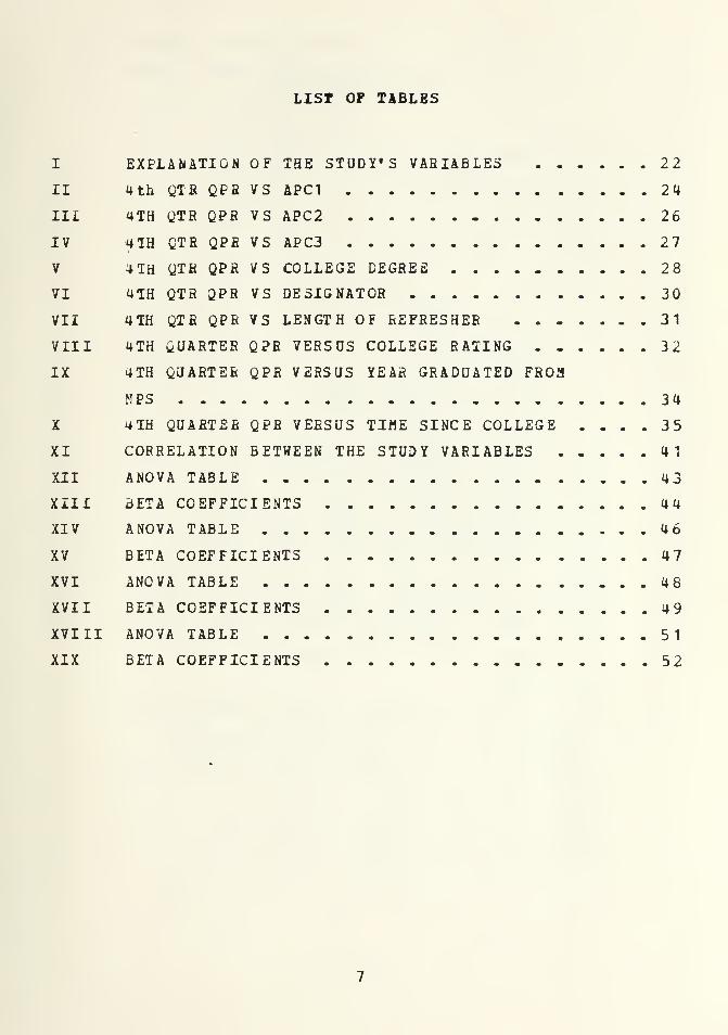
LIST OF TABLES

I EXPLANATION OF THE STUDY'S VARIABLES 22

II 4th QTR QPR VS APC1 24

III 4TH QTR QPR VS APC2 26

IV 4TH QTR QPR VS APC3 27

V 4TH QTR QPR VS COLLEGE DEGREE 28

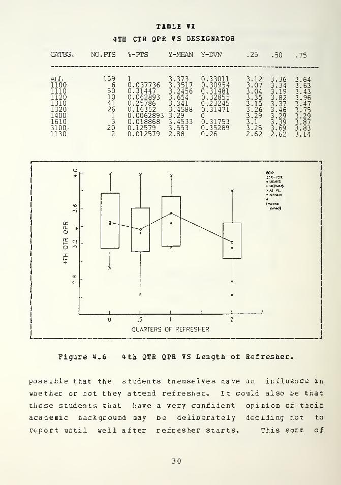
VI 4TH QTR QPR VS DESIGNATOR 30

VII 4TH QTR QPR VS LENGTH OF REFRESHER ....... 31

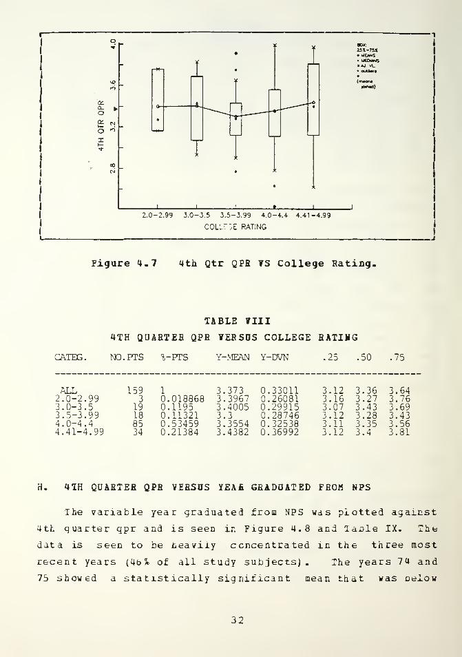
VIII 4TH QUARTER QPR VERSUS COLLEGE RATING 32

IX 4TH QUARTER QPR VERSUS YEAR GRADUATED FROM

NPS 34

X 4IH QUARTER QPR VERSUS TIME SINCE COLLEGE .... 35

XI CORRELATION BETWEEN THE STUDY VARIABLES 4 1

XII ANOVA TABLE 43

XIII BETA COEFFICIENTS 44

XIV ANOVA TABLE 46

XV BETA COEFFICIENTS 47

XVI ANOVA TABLE 48

XVII BETA COEFFICIENTS 49

XVIII ANOVA TABLE 51

XIX BETA COEFFICIENTS 52

LIST OF FIGURES

2.1 Calculating APC's 13

3.1 AFC Main Effects 18

3.2 College Rating 19

3.3 College Degree 20

3.1 Length of Refresher 21

3.5 Designator .........214.1 4th QTR QPR VS APC1 23

4.2 4th QTR QPR VS APC2 25

4.3 4th QTR QPR VS APC3 26

4.4 4th QTR QPR VS College Degree 28

4.5 4th QTR QPR VS Designator 29

4.6 4th QTR QPR VS length of Refresher 30

4.7 4th Qtr QPR VS College Rating 32

4.8 4th QTR QPR VS Year Graduated from NPS 33

4.9 4th Quarter QPR Vs Time Since College 34

5.1 Plots of Residuals from the Study Model of

Choice 38

5.2 Residual Plot and Data :Study Model 39

5.3 Scatter Plot of Residuals :Study Model 40

5.4 Two Cofactor and Six M/E Model with

Interactions 43

5.5 Two C/F and Six M/E Model without Interactions . . 46

5.6 4 Cofactor and 3 M/E Model with Interactions ... 48

5.7 4 Cofactor and 3 M/E Model without Interactions . . 50

D.1 6th Qtr Grad QPR vs APC1 64

D.2 8th Qtr Grad QPR vs APC1 65

D.3 8th Qtr Iotal QPR vs APC1 66

D.4 6th Qtr Gcad Q^E vs APC2 67

D-5 8th Qtr Grad QPR vs APC2 68

D.6 8th Qtr Total QPR vs APC2 69

D.7 6th Qtr Grad QPR vs APC3 70

D. 8 8th Qtr Grad QPR vs APC3 71

D.9 8th Qtr Total QPR vs APC3 72

D. 10 6th Qtr Grad QPR vs College Degree 73

D. 1 1 8th Qtr Grad QPR vs College Degree 74

D.12 8th Qtr Total QPR vs College Degree 75

D. 13 6th Qtr Grad QPR vs Designator 76

D. 14 8th Qtr Grad QPR vs Designator 77

D.15 8th Qtr Total QPR vs Designator 78

D. 16 6th Qtr Grad QPR vs Length of Refresher 79

D.17 8th Qtr Grad QPR vs Length of Refresher 80

D- 1

8

8th Qtr Total QPR vs Length of Refresher 8 1

D. 19 6th Qtr Grad QPR vs College Rating 82

D.20 8th Qtr Grad QPR vs College Rating 83

D. 2

1

8th Qtr Total QPR vs College Rating 84

D.22 6th Qtr Grad QPR vs Year Graduated NPS 85

0,23 8th Qtr Grad QPR vs Year Graduated NPS 86

D.24 8th Qtr Total QPR vs Year Graduated NPS 87

D.25 6th Qtr Grad QPR vs Time since College 88

D.26 8th Qtr Grad QPR vs Time Since College 89

D.2 7 8th Qtr Total QPR vs Time Since College 90

I- INTROEOCTIOM

The purpose of this thesis was to investigate various

factors affecting the academic performance of Naval Officer

students in the Operations Analysis Curriculum at the Naval

Postgraduate School. The original goal was to arrive at a

predictive model which would improve the present selection

process and possibly reduce the numbers of student academic

transfers out of the Operations Analysis Curriculum. These

transfers have historically been about 10S of the original

class. Due to the relatively small sample size (159), it

was not possible to cross validate . Because of this the

results are not presented as a predictive model. The

utility of the study is rather in its analysis of those

factors influencing the student's academic performance; the

resultant promotion of understanding, and suggestions for

farther study of the subject.

The pertinent variables that were readily available and

are in this study are college QPR, college degree, the

Officer's designator, college quality rating, elapsed time

from conpleticn of college to starting the Operations

Analysis Curriculum, year graduated from the GA Curriculum,

and the length of refresher attended it the Naval

Postgraduate School. Current practice using only the "APC"

codes as a predictor achieves a multiple correlation coeffi-

cient of .21 when run through the ANOVA package. The model

recommended in the study has an R 2 of .41 while another

model achieves an R 2 as high as .53.

The study subjects include approximately one-half of the

Navy OA graduates from the period 1974 to 1985. This was

the case since APC's were only available for about one-half

of the graduates. The study includes only those students

10

witn academic profile codes of 435 or better. The recom-

mended APC for the Operations Analysis Curriculum is 324 or

better. There were 43 individuals included in the study

whose APC was ,at least in one of the three digits, outside

that recommended for OA. Cf these 43 ptople, 6 went

straight into the curriculum without any refresher.

A review of the literature reveals a thesis written by

Heru Soetrisno in 1975 titled "Prediction of Academic

Performance of the U. S. Navy Officer Students in the

Operations fcesearch/Systems Analysis curriculum at the Naval

Postgraduate School" [fief. 1 ]• The study was a regression

analysis using biographical data, a personal interest survey

and the graduate record examination- It covered all the

Navy students in OA in the Spring of 1974 (72 students)

.

The thesis concluded that tne three above mentioned vari-

ables and combinations of them were better predictors of

student performance than undergraduate QPR and college

guality.

Numerous articles have also been written concerning the

subject of predicting academic performance. A review of

many of these articles has left the author with the impres-

sion that it is clearly not a clean-cut issue as to what

test cr measure is the best in predicting academic perform-

ance. However of all the choices, it is recognized that

prior academic performance and aptitude tests are generally

considered to the most important predictors of future

academic performance [Bef. 2: page 10 ]•

The study opens with the development of the academic

profile code and a review of the data. The analysis is

conducted by first a preliminary look at the independent

variables in relationship to the dependent variable and then

with an analysis of variance technique. The study ends with

several conclusions and recommendations for future

consideration.

1 1

II. BACKGHOOHD

The Navy Military Personnel Command (NMPC) is respon-

sible for filling quotas at the Naval Posgraduate School.

The current procedure is to convene annually a Graduate

Selection Board £Re£. 3]. This board meets and reviews

those Officer's records who are potentially eligible for

graduate education as shown in enclosure four of [fief. 3].

The beard bases their determination for possible graduate

education on the Officer's professional performance and

their academic ability as evidenced by their academic

profile code (APC) [ Bef . 4]. The most recent board screened

13,000 records and selected 4,000 for possible graduate

studies- Approximately 90% of those students eventually

completing fully funded graduate studies will receive their

degrees from the Naval Postgraduate School [ Eef . 5: page

25].

The APC is a three digit code summarizing the previous

education of each Officer and is calculated as seen in

Figure 2.1 .

Appendix B is a sample academic record evaluation (ARE)

sheet. The ARE is used by the director of admissions at the

Naval Postgraduate School as a worksheet to compute an APC

for every newly designated Naval Officer each year. The ARE

is filed and maintained at the Director of Admission's

office at the Naval Postgraduate School and is kept on file

until the Officer has been designated as a subspecialist or

has teen determined not suitable for graduate education.

NMPC annually directs the Naval Postgraduate School to

remove and destroy the ARE's for those above mentioned

Officers.

12

QPR CODE MATH CODE

(1st APC Diqit) (2nd APC njnit)

(Code # Grade QPR Range Code # Calculus-Relate^ Math Courses

A-/A 3.60 - 4.00 Siqnificant Dost-calcul us math with

1 B* 3.20 - 3.59 B averaqe2 B-/B 2.60 - 3.19

3 C-f 2.20 - 2.59 1 Two or more calculus courses with

4 C 1.90 - 2.19 B* averaqe

5 Below C 0.00 - 1.89

2 Two or more calculus courses with

{Repeated courses and failures O averaqe

I are included in the QPR calcu-

I

Nation.) 3 One calculus course withC grade or better

| 4 Two or more ore-calculus courses with

B average or better\

jS At least one ore-calculus course with

| C qradeI

j 6 No col leqe-level math with C qrade

l!

I

I

|

j TECHNICAL CODE(jrd APC Diqit)

I

jSiqnificant Upper-Division Course

jCoveraqe in a Pertinent Fnqmeerinq

ICode # Physics (Calculus-Based) or Physical Science Discipline

I

1 > B* averaqe

1

2 Complete sequence taken withB+ averaqe

C+ averaqe

3 Complete sequence taken withC* averaqe

4 At least one course withC grade

5 None

Figure 2.1 Calculating APC's.

13

The APC is originally based on the individuals college

performance and rarely changes unless the individual corre-

sponds with the Director of Admissions at tne Naval

postgraduate School and petitions to raise (improve) his APC

with written proof of additional accredited academic

achievement [Bef. 4: page 11].

A Naval Officer must possess an APC of 324 or better

(e.g. 112) to directly enter the Operations Analysis

Curriculum [fief. 5: page 32]. Additionally, a Naval Officer

may enter the OA Curriculum with an APC of 344 after

completing one or twc quarters of the Engineering Science

Curriculum. The Engineering Science Curriculum is designed

to provide an opportunity for Officers with madeguate math-

ematical and physical science backgrounds to establish a

good math foundation to be able to qualify for a technical

curriculum [Ref. 5: page 36]. There is also a six week

refresher available that is designed to rapidly cover the

calculus and physics fundamentals for those Officers who are

direct inputs into the OA curriculum without any quarters of

Engineering Science. Exceptions are made and it is possible

for an individual to enter the OA curriculum without the

minimum APC. It is also possible for an Officer to start OA

without any refresher at all as did 63 of the study

sub jects.

The OA curriculum is of a technical nature and students

with solid college performance and technical majors are

encouraged to enroll in it. However, there are some very

good professional Officers who do not have the required

academic background to directly enroll in OA. The Navy

would like some of these Officers to be able to attend NPS

in a technical curriculum . In response to this need, the

Navy has recently introduced (1985) tne Technical Transition

Program (TTP)

.

This program is designed to allow those

professionally exceptional officers with weak college

14

backgrounds to enter a technical curriculum via a one or two

quarter individually tailored preparation program. Tnis

program is slightly different from the Engineering Science

curriculum in that it is individually structured to meet

each student's needs while it also varies from different

curriculum to curriculum. This program not only provides an

opportunity to Officers that at one time had no or little

hope cf attending the Naval Postgraduate School but it also

provides more graduate trained subspecialists for the Navy.

The college records of these candidates for the TTP are

screened at the Naval Postgraduate School and a decision is

made whether or not to allow an individual to start the

program in hopes of eventually entering a technical curric-

ulum. This study reveals several important factors and

considerations in order to help the decision maker better

access the potential academic performance of future OA

students.

15

III. DISCUSSION OF THE DATA

The study data was gathered from several sources

including the Office of the Registrar, Director of

Admissions, the Operations Analysis Curricular office at the

Naval Postgraduate School and from the Naval Kilitary

Personnel Command. Most of the data was obtained from the

individual student files maintained by the operations

Analysis curriculum secretary. These files contained much

of the student data such as university attended and what

dates attended, college degree, designator and length of

refresher attended at the Naval Postgraduate school. These

same files contain the students grade sheet summary of all

course %orlc completed at the Naval Postgradute School. From

this sheet, the dependent variable in the study was calcu-

lated. Four different guality point ratings (QPB) were

studied. The first was the student's total grade average

after four quarters of the Operations Analysis Curriculum.

This grade is of special importance as it is at this point

in the curriculum that a final decision must be made as to

continue a marginally performing student in nopes that his

overall grade point average will improve or to allow him to

possifcly transfer to another curriculum with enough time

remaining to successfully complete that program- It is also

important to note that through the first four quarters each

option is essentially the same. Hence, there is uniformity

in the program. If a model cculd be constructed that would

improve the present selection process and reduce the numbers

of these transfers, a savings in time and money could be

realized by the Navy.

The three other dependent variables looked at were the

student's quality point rating after six quarters (when most

16

of the stringent course requirements are finished), his

graduate gpr after eight quarters and also the total overall

quality point rating after eight quarters which completes

the degree- All these qpr' s were determined by dividinq the

weiqhted total of the qrade points earned by the total hours

attempted for the respective quarter totals. None of these

qpr's included any qrades earned durinq refresher courses.

The academic profile codes were the most difficult data

points to obtain. Althouqh the Director of Admissions main-

tains a computer printout of all current APC's, very few of

tne study subjects were still on the listinq. Of the 343

Navy CA students completinq the Operations Analysis curric-

ulum at the Naval Pcstqraduate School from 1974 to 1985,

only 60 of them had APC's in the printout, in their files or

in their academic record evaluation sheets. The additional

APC's were obtained from the Officer's data card sent to the

Naval Postqraduate School by NMPC. A total of 172 APC's

were obtained. Of these 172 APC's, 159 were used in the

study. The thirteen individuals removed from the study were

in very low populated levels of several of the variables.

The variables for the academic profile codes are seen in

Fiqure 3.1 .

The 159 Naval Officer study subjects all qraduated with

Master Deqrees in Operations Analysis. Althouqh not a

random sample, they were treated as a random sample for the

purpose of the study. There was no apparent qrouping or

special distribution of the study subjects compared to the

entire population of 3H3. The data were tabulated into an

159 by 18 matrix and is included as Appendix C.

The variable colleqe rating was obtained from the

Gourman Report [fief. 6: page 7]. This report evaluated

1,845 colleges and universities in terms of the institu-

tion's objectives, curriculum, faculty, faculty research and

honors, administration, library, budget, resources, student

17

r

APC1 = College QPR

code main effect level # of data points

1 812 28

2 3 79

3 4 39

4 5 5

total 159

APC2 = Math Code

code main effect level # of data points

1 2412 29

2 3 7613 4 30

1

I

total 159

APC3 = Technical Code

code main effect level # of data points

1 412 19

2 3 25

3 4 59

4 5 39

5 6 13

total 159

Figure 3. 1 APC Main Effects.

scores on standardized tests, admission policy, and several

other tactors. Tne range for the college rating variable as

18

a cofactor was 4.99 for the highest rated institution down

to a rating of 2.01 for the lowest. This variable was also

looked at as a possible main effect and was divided into

categories as seen in Figure 3.2 .

rating range level # of data points

34

85

18

19

3

strong 4 41-4.99 6

good 4 01-4.40 5

acceptable 3 .51-3.99 4

adequate 3 01-3.50 3

marginal 2 .01-2.99 2

total 159

Figure 3.2 College Bating.

The variable college degree is seen in Figure 3.3 . The

grouping Naval Science was reguired due to the twelve

students included in the study who graduated from the Naval

Academy prior to 197 3. Prior to that rime only one degree

was confirmed by the institution and although the midshipmen

took a variety of courses, many of wnich were of an engi-

neering nature, they received a B. S. degree in Naval

Science.

The variable refresher was investigated as botn a main

effect (yes=attended cr no=did not attend) and as a cofactor

listing the length, in quarters, of refresher taken at the

Naval Postgraduate School. There is a six week rerresher

for each class prior to starting the curriculum.

Additionally, a student may possibly receive one or two

quarters of refresher depending on several factors- These

quarters of refresner are generally undertaken by students

19

I Degree

Business

Engineering

Humanities

Math

Social Science

Naval Science

Operations Analysis

level

1

2

3

4

5

6

7

# of data points

14

31

4

59

16

12

23

total 159

Figure 3.3 College Degree.

not meeting the minimum recommended APC for OA or for

students who have not been in an academic environment for a

long period of time. The decision is generally made at the

Curricular Officer and Academic Associate's concurrence and

with approval from the student's detailer. There is nothing

concrete aoout this process and it is possible to start the

curriculum directly without any refresher. The cofactor

length of refresher was grouped as seen in Figure 3.4 .

The variable designator was viewed as a main effect.

£ach Naval officer has one designator which is generally

assigned after completing a school or training course. They

retain this designator for their entire length of service

with the few exceptions of individuals transfering to

another specialty and hence changing designators. The

designators of tne study group can be seen in Figure 3. 5 .

Table I is a summary listing of all tne variables and

their levels that were investigated in the study.

20

,—

.

.,— -,

quarters of Refresher level # of data points

1 63

.5 2 58

1 3 8

2 4 30

total 159

Figure 3.4 Length of Refresher.

Jdesignator definition level # of data pts

I

llOx restricted line 1 6

J lllx unrestricted line 2 50

]112x submarines 3 10

|131x aviator 4 41

J

132x naval flight officer 5 26

|140x engineering duty 6 1

|161x intelligence 7 3

j310x supply 8 20

j113x special warfare 9 2

J

total 159

Figure 3.5 Designator.

21

TABLE I

EXPLANATION OF THE STUDY'S VARIABLES

Cofactors Values

time since college in months 23-178

college rating 2.01-4.99

year graduated from NPS 74-85

length of refresher (quarters) 0, .5, 1, 2

Main, Effects Level

APC1 college qpr * 1,2,3,4,5

APC2 math code * 1,2,3,4

APC3 technical code * 1,2,3,4,5,6

College Degree Level

Business 1

Engineering 2

Humanities 3

Natural Science (Math) 4

Social Science 5

Naval Science 6

Operations Analysis 7

Designator Level

llOx Restricted line 1

lllx Unrestricted line 2

112x Submarines 3

131x Aviator 4

132x Naval flight officer 5

140x Engineering Duty officer 6

161x Intelligence officer 7

310x Supply officer 8

113x Special Warfare officer 9

- Coded as APC + 1 for computer indexing

22

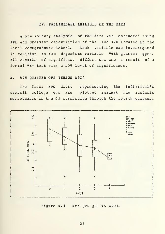
IV. P&ELIHIMIET ANALYSIS OF THE DATA

A preliminary analysis of the data was conducted using

APL and Grafstat capabilities of the IBM 370 located at the

Naval Postgraduate School- Each variable Mas investigated

in relation to tne dependent variable "4th quarter qpr".

All remarks of significant differences are a result of a

formal "t" test with a .05 level of significance.

A. 41H QUARTER QPfi VERSOS APC

1

The first APC digit representing the individual's

overall college qpr was plotted against his academic

performance in the OA curriculum through the fourth quarter.

o

2

APC1

BOX:

ut-m• UtMIS• utowfi»AJ W.

Join*)

Figure 4.1 4th QTB QPR VS APC1.

23

Figure 4.1 is a graphical representation of the statistical

relationsnip while the results are tabulated in Table II.

TABLE II

4th QTfi QPB ¥S APC1

CATEG. NO.PTS %-PTS Y-MEAN Y-DVN .25 .50 .75

ALL 159 1 3.373 0.33011 3.12 3.36 3.648 0.050314 3.72 0.24068 3.43 3.63 3.96

1 28 0.1761 3.5386 0.27132 3.36 3.47 3.752 79 0.49686 3.3448 0.3088 3.09 3.34 3.593 39 0.24528 3.2826 0.32053 3.07 3.25 3.464 5 0.031447 3.042 0.34672 3.02 3.11 3.15

These results show the student's performance in college has

a direct and logical relationship to his performance through

the fourth guarter of the OA curriculum. The higher one's

college gpr tne better one's performance in OA. The study

group's average APC for the first digit is very close to two

wnile the overall grand mean for their fourth quarter grade

was 3.37. The highest code of zero had a significant

difference compared to the overall mean.

B. 41H QUARTEfi QPB VERSUS APC2

The second APC digit representing the student's under-

graduate calculus proficiency was plotted against his 4th

guarter gpr. Figure 4.2 is a representation of this rela-

tionship and the numerical results are tabulated in Table

III. There is a significant difference among tne first two

levels of this variable and the overall mean. The recom-

mended APC for OA in math is three or better while four is

acceptable via the engineering science curriculum. The

study group's average was 1.7 while the entire group had a

math APC of three or better- Tne overall relationsnip is

24

just a slignt positive one where the lower (better) one's

math code translates to a higher 4th quarter grade.

C. 41H QUARTEB QPB 7EBS0S APC3

a:a.o

o

::

1

o *

f

;t

::

t~ —

o

*

BOX.-

23X-7J*• UCAHS» mown»AJ VI.

• IXXJ4.II

•

Jo**)

APC2

Figure 4.2 4th QTR QPB YS APC2.

The thira APC digit representing the students tecnnical

code was similary studied and is shown Figure 4.3 and Table

IV. This relationship does not show a logical progression

of high 4th guarter performance with the better technical

codes. It in fact jumps back and forth with no apparent

logic. Admission to the CA curriculum Eay reflect some

compensating feature.

The last level (those students with an APC3 code of

five) of thirteen individuals had the second best average

gpr. Tnese thirteen subjects were looked at individually to

25

TABLE III

4TH QTR QPB ?S APC2

CATEG. NO.PTS %-PTS Y-MEAN Y-DVN .25 .50 75

ALL 59 1 3.373 0.33011 3.12 3.36 3.6424 0.15094 3.4963 0.26836 3.29 3.43 3.7529 0.18239 3.5034 0.2918 3.29 3.59 3.776 0.47799 3.3143 0.32307 3.08 3.3 3.4930 0.18868 3.297 0.3607 3.03 3.22 3.58

to

a:

o **

X

-L

2 3

APC3

BOX:

m-71X• uixiS• uEOMS»*J. A.

•

Figure 4-3 4th QTE QPR VS APC3.

try to determine a possible reason for this. It was discov-

ered, that as a group, their average first digit APC for

tneir college performance was 1.4. This is much tetter than

the entire study group's average of 2. 1. The only differ-

ences between the six level means and the overall mean that

26

TABLE IT

4TH QTB QPB ?S APC3

CATEG. NO.PTS %-PTS Y-MEAN Y-DVN .25 .50 75

ALL 159 1 3.373 0.33011 3.12 3.36 3.644 0.025157 3.705 0.17642 3.5 3.59 3.77

1 19 0.1195 3.4511 0.33468 3.05 3.46 3.792 25 0.15723 3.3636 0.29094 3.1 3.29 3.63 59 0.37107 3.3958 0.29821 3.16 3.36 3.634 39 0.24528 3.2379 0.3671 3.96 3.26 3.465 13 0.081761 3.4769 0.27921 3.29 3.46 3.73

were statistically significant were the first level zero and

the next to last level four.

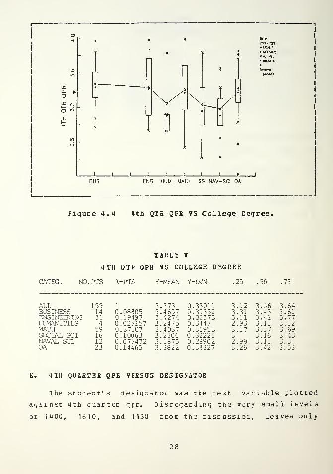
O. 4TH QUABTEE QPB TEBSDS COLLEGE DEGBEE

College degree was the next variable plotted against the

4th guarter gpr. Figure 4.4 graphically presents and Table

V lists this data.

Althougn none of the differences are statistically

significant, the business, engineering, math and operations

analysis majors performed above the mean of the study

sample. If one disregards an outlier or two within the OA

level, CA would have shown a greater positive difference

from the grand mean and this can be seen in its inter-

guartile range. The data shows an intuitively logical

assumption that students with a social science or humanities

undergraduate degree would do less well in a technical

curriculum when compared to students with a more quantita-

tive college degree such as engineering or mathematics. The

performance of those people with naval science majors is

relatively low. This may be a result of several confounding

factors not readily apparent.

27

BU'

* "• :

y.

-'

• 3

'X>

onao

>• "v

8

>

<>

:

*

*

•

5 :

ri> :

X

•

3 t •

1 1 1 1 1 1 1 1 • 1

ENG HUM MATH SS NAV-SCI OA

BOX-

23X-73T• uc vil• utowrs»*J A.

(l

)««•<»

Figure 4.4 4th QTB QBE ?S College Degree,

CATEG.

TABLE ¥

4TH QTB QPR VS COLLEGE DEGREE

NO.PTS %-PTS Y-MEAN Y-DVN .25 50 75

ALL 159 1 3.373 0.33011 3.12 3.36 3.64BUSINESS 14 0.08805 3.4657 0.30352 3.31 3.43 3.61ENGINEERING 31 0.19497 3.4274 0.32373 3.11 3.41 3.77HUMANITIES 4 0.025157 3.2475 0.3447 2.93 3.11 3.12MATH 59 0.37107 3.4037 0.31953 3.17 3.37 3.69SOCIAL SCI 16 0.10063 3.2306 0.32225 3 3.16 3.43NAVAL SCI 12 0.075472 3.1875 0.28902 2.99 3.11 3.3OA 23 0.14465 3.3822 0.33327 3.26 3.42 3.53

E. 4TH QUABTEB QPB VERSOS DESIGNATOR

The student's designator was the next variable plotted

against 4th quarter qpr. Disregarding the very small levels

of 1400, 1610, and 1130 from the discussion, leaves only

28

1120 (submariners), 1320 (naval flight officers) and 3100

(supply) designators that did better than the grand mean.

This can be seen in Figure 4.5 and Table VI. A test of

significance showed only the 112 and 3100 designators

performed better and the 1100 designator performed worse

than the overall mean.

&

O ">

Xh-

oo

CM

: t

L i

: n AJL

/V

»

(

<

A 1

'*

h 4

,/'

-_ c

3 ;

'\>

I

T

-

>

1 ! 1

c

I 1 !

1100 1110 1120 1310 1320 1400 1610 3100 1130

DESIGNATOR

BOX:

2JX-71X

» *j w.• ouuwit

(m*on»

Figure 4.5 4 th QTR QPR ?S Designator.

P. 4TH QUARTEB QPB VERSUS LENGTH OF REFRESHER

The variable length of refresner was plotted against 4th

quarter gpr as seen in Figure 4.6 and Table VII.

It can be seen that those individuals who do not attend

refresher do slightly better than tne students that attend

refresher. This could mean that a good job is done identi-

fying those individuals who need refresher. It is also

29

CATEG.

TABLE ?I

41H CTfl QPE ?S DESIGHATOfi

NO.PTS %-PTS Y-MEAN Y-DVN 25 50 .75

ALL 159 1 3.373 0.33011 3.12 3.36 3.641100 6 0.037736 3.3517 0.30954 3.07 3.34 3.631110 50 0.31447 3.2456 0.31481 3.04 3.19 3.431120 10 0.062893 3.654 0.32855 3.35 3.82 3.961310 41 0.25786 3.341 0.23245 3.15 3.37 3.471320 26 0.16352 3.4588 0.31471 3.26 3.46 3.751400 1 0.0062893 3.29 3.29 3.29 3.291610 3 0.018868 3.4533 0.31753 3.1 3.39 3.873100,* 20 0.12579 3.553 0.35289 3.25 3.69 3.831130 2 0.012579 2.88 0.26 2.62 2.62 3.14

*"

:

-

j'

: :

*

'O

»--

O-

•

-

•

•f

Jc

; :

- , c •

i i i I 1 1

.5 1

QUARTERS OF REFRESHER

BOX

m-73*• UCWIS• ufniw<s

»*J A.• oirtlWrt

•

(mtant

Figure 4.6 4th QTB QPR VS Length of fiefresher.

possible that the students tnemseives nave an influence in

wnether or not they attend refresher. It could also be that

those students that have a very confident opinion of their

academic background may be deliberately deciding not to

report until well after refresher starts. This sort of

30

TABLE ¥11

41H QTB QPB ?S LENGTH OP REFRESHER

CATEG. NO.PTS %-PTS Y-MEAN Y-DVN ,25 .50 ,75

ALL 159 1 3.373 0.33011 3.12 3.36 3.6463 0.39623 3.441 0.33443 3.15 3.42 3.77

0.5 58 0.36478 3.3597 0.32014 3.11 3.32 3.61 8 0.050314 3.54 0.29039 3.17 3.43 3.732 30 0.18868 3.2117 0.28024 3.03 3.15 3.43

biased selection coald be affecting the results of this

variable. The result of the students with one quarter of

refresher doing better than the mean could also be artifi-

cial, once they demonstrated that even though they fit the

category of individuals who should get refresher, they

really could handle the pace without it then they could be

set tack into their original class with a few scheduling

arrangements made. There is also no permanent incentive to

do well in the 460 curriculum since the grades do not count

and are not reflected in the student's total grade average-

The formal test of significance showed that oniy the

students with two guarters of refresher performed at a

statistically lower level than the overall grand mean.

G. 47H QUARTER QPB ?£RS0S COLLEGE RATING

The variable college rating was the next variable

plotted against 4th guarter qpr and is shown in Figure 4.7

and Table VIII. The data does not show a significant

difference among any of the college ratings. Disregard the

lowest rating as it only contains three individuals. The

remaining four categories shew a slight decrease in 4th

guartei gpr as the rating decreases but it is not statisti-

cally significant.

31

to

o ">

n r

-H-

SOX2SX-73X• utwS. UCDUNS«*J W.

io*w*a

2.0-2.99 3.0-3.5 3.5-3.99 4.0-4.4 4.41-4.99

COLLtOE RATING

Figure 4.7 4th Qtr QPE TS College Rating.

CATEG.

TABLE fill

4TH QUABTEB QPE ¥ERSDS COLLEGE EATIHG

NO.FTS %-FTS Y-MEAN Y-DVN .25 .50 .75

ALL 159 1 3.373 0.33011 3.12 3.36 3.642.0-2.99 3 0.018868 3.3967 0.26081 3.16 3.27 3.763.0-3.5 19 0.1195 3.4005 0.29915 3.07 3.43 3.693.5-3.99 18 0.11321 3.3 0.28746 3.12 3.28 3.434.0-4.4 85 0.53459 3.3554 0.32538 3.11 3.35 3.564.41-4.99 34 0.21384 3.4382 0.36992 3.12 3.4 3.81

H. 41H QDAETEE QPE VEESOS YEAfi GBADOATED FROM NPS

The variable year graduated from NPS was plotted against

4th quarter qpr and is seen in Figure 4.8 and Tai)le IX. The

data is seen to be neavily concentrated in the three most

recent years (4b % of all study subjects). The years 74 and

75 showed a statistically significant mean that was oeiow

32

the overall mean of 3.37- The year 1980 was the only year

that was significantly above the overall average- This

could possibly reflect the "luck of the draw" as different

student sections progress through the curriculum with

different combinations of professors and grading practices.

74 75 76 77 78 79 80 81 82 83 84 85

YEAR GRADUATED FROM NPS

Figure 4.8 4th QTR QPB ?S lear Graduated from NPS.

I. 4TH QUARTEB QPH ?EHSOS TIME SINCE COLLEGE

Ihe variable time since college was plotted against the

4th guarter qpr as seen in Figure 4.9 and Table X.

After discarding the first level with only two observations,

it is of interest to note the very slight improvement in qpr

as tiae since college increases. Once again the differences

between the overall mean and the individual level means are

not significant in a formal test of significance. The

33

TABLE II

41H QUAETEfi QPB YEBSOS YEAB GRADUATED PBOM NPS

CATEG. NO.PTS %-PTS Y-MEAN Y-DVN 25 .50 75

ALL 159 1 3.373 0.33011 3.12 3.36 3.641974 8 0.050314 3.1388 0.24174 3.04 3.11 3.291975 12 0.075472 3.1825 0.25898 2.99 3.09 3.311976 7 0.044025 3.4314 0.25525 3.08 3.5 3.591977 7 0.044025 3.47 0.21024 3.22 3.45 3.671978 2 0.012579 3.515 0.085 3.43 3.43 3.61979 14 0.08805 3.3514 0.33939 3.03 3.36 3.531980 9 0.056604 3.6178 0.21186 3.58 3.69 3.761981 '* 11 0.069182 3.2918 0.28074 3.1 3.15 3.481982 15 0.09434 3.4433 0.39383 3.27 3.56 3.761983 31 0.19497 3.3881 0.355 3.08 3.39 3.71984 27 0.16981 3.3441 0.2765 3.14 3.32 3.471985 16 0.10063 3.4381 0.37902 3.26 3.43 3.82

orCL

oKi—

O

o

f i

-< »

t ^f

|-W

< i

i

5

f

fQ

-0 \ ' -«

Jr

1 -<,

-

J

J 1

-

0-36 37-60 61-84 85-108 109-132 133-185

TIME SINCE COLLEGE IN MONTHS

BOX23X-73X

• mown« Kl A.

Figure 4.9 4th Quarter QFB Vs Time Since College.

relative constant performance over tris vanafcle is

surprisinq as one would logically expect performance to be

degraded as the time since completing college and commencing

another academic situation increases.

34

TABLE I

4TH QUARTEB QPH VERSOS TIME SINCE COLLEGE

CATEG. NO.PTS %-PTS Y-MEAN Y-DVN .25 .50 .75

ALL 159 1 3.373 0.33011 3.12 3.36 3.640-36 2 0.012579 3.595 0.165 3.43 3.43 3.7637-60 58 0.36478 3.3 0.30956 3.11 3.29 3.4761-84 38 0.23899 3.4037 0.34813 3.11 3.39 3.6785-108 27 0.16981 3.38 0.35614 3.1 3.38 3.64109-132 19 0.1195 3.4516 0.29108 3.14 3.48 3.76133-185 15 0.09434 3.436 0.31117 3.12 3.34 3.79

The preceeding relationships were xooked at to investi-

gate the basic properties of the variables studied and r.ot

to draw conclusions on these results. It would be incorrect

to draw the conclusion that tnese one to one comparisons

imply any direct cause and effect without studying the

interactions of all the variables concerned. Chapter V will

investigate these relationships with an analysis of variance

approach. Appendix D contains the same figures and tables

for the other three dependent variables (6tn guarter grad-

uate gpr, 8th guarter graduate total gpr and 8th guarter

total gpr) .

35

?. BESOLTS OP TBE ANALYSIS

A. APPflOACH OF THE ANALYSIS

This chapter describes the analysis techniques used and the

results from the analysis. The analysis of the data was

conducted with the aid of the Naval Postgraduate School's

IBM 370 computer using an "ANOVA" package designed by

Professor Eussell Richards of the Naval Postgraduate School.

The "ANOVA" package is capable of performing multiple-

linear regression on unbalanced data. It is an APL program

with nany and varied outputs. Appendix E is an explanation

of the "ANOVA" program, its capabilities and required input

data format. The program uses the least squares approach

and calculations are done in matrix format.

All of the 159 students that comprised the population of

this study were included in the analysis to develop a model

for possible prediction of student performance. A cross

validation procedure, using a portion of the data, would

have reen a useful technique to check the validity of the

results. This procedure was not employed due to the limited

number of academic profile codes tnat were available for the

study.

B. MULTIPLE LINEAfi REGRESSION ANALYSIS

Multiple linear regression techniques were employed

usinq the "ANOVA" prcqram to develop tne explanatory vari-

ables to be included in the model and then to estimate the

coefficients describing the weights to assign to the

variables.

36

C. HCDEL

The model used is of the matrix form;

Y = XB «•€ {eqn 5. 1)

where, Y is a vector of dependent variables

X is a matrix of independent variables

B is a vector of coefficients

e is a vector of error terns.

In ANOVA applications of linear models, the qualitative

(main and interaction) effects are estimated on an interval

scale and have arbitrary origins. Hence the matrix X is

singular. The "ANOVA" package (Professor Richards) solution

manages this problem by deletion of selected columns and

these selected columns are listed for the user. A selected

column represents an omitted variable whose estimated coef-

ficient is the negative of the total of all other variables

in its category.

D. ASSUBPTIOMS FOB LIMElfi REGRESSION

While using the linear regression approach, a number of

assumptions must be made concerning the error terms. The

errors must be independent, have zero mean, constant vari-

ance and must be normally distributed [ Ref . 7]. Each time

the "ANOVA" program was run on a different version of the

model the residuals were plotted to verify these assump-

tions. Figure 5.1, Figure 5.2 and Figure 5.3 display these

results for the particular model that will later be devel-

oped as the study model of choice. These figures and the

discussion in the following paragraph show the assumptions

are adequately met.

The variables included in the model must also be inde-

pendent. The Peacsoa's product moment correlation

37

NORMAL DENSITY FUNCTION, N=159

-0.4 0.4

RESIDUALS FROM 4TH OTR MODEL

NORMAL CUMULATIVE DISTRIBUTION FUNCTION, N=159

-0.4 0.4

RESIDUALS FROM 4TH OTR MODEL

0.8

J

Figure 5-1 Plots of fiesiduals from the Study Model of Choice.

38

NORMAL PROBABILITY PLOT

9900

99 00

93.00

90 00

^3 00

zIJO 00oen

^3 00

1000

300

too

,.

-0

r

i

.'

i

.'

1*X '

i

•

•

__L » j l y^j-i

i

i >

L 1 j \..i±l t

1

1

i 1

1

1

i

r

i >-^;

'

"""1

i

i

i

L I..jz.j l l :.

r 1r :

l

i

t

S\ 1 1 1 1 1 i

i

i

-0.4 0.4

RESIDUALS FROM 4TH QTR MODEL0.8

NORMAL DISTRIBUTION

X : DOSELECTiaM : ALLLABEL : RESIDUALS FROM 4TH QTR UDOCLSAMPLE S IZE: 139

MINIMUM - 559MAX1MM 629CENSORIM) : NONEEST. ICTI 00: UAXIMLM LIKELIHOOD

SAMPLE FITTEDMEAN 1 .4820E-M 1.4620E-14STD DEV 2.5409E"! 25409E-ISkEWHESS 1.8I56E-1 o.ooooeoKURTOSIS 2.5538E0 3O000E0

PERCO/TIl ES SAMPLE FITTED5: -0.37343 -4 1804E-1

10: -0.31989 "3.2568F-125: -0. 18633 -I.7I31E-I50: -0.0083107 25665E-875: 0.18291 1.7131E-I90: 0.35343 3.2368E-195: 0.48034 4.1804E-I

COVARIAJICE MATRIX OFPARAMETER ESTIMATES

MU SIGMAMU 00040351SIGMA 00020303

KS. AD. AJC CV SIGNIF. LEVELS NOT EXACT WITH ESTIMATED

0.93 C0NF1DDCE INTERVALSPARAMETER ESTIMATE LOWER UPPERMU 1.4820E-14 -0 039379 039378SIGMA 2.5409E-1 2289 0.28557

COOOHESS OF FITCHI-SOUARE 2 8393

DEO TREED 5

SIGHIF 0.72474KOIU-CMIRN 044604

SIGNIF 0.90979CRAWfR-V M 0.021326

SIGHIF > .13

ANOER-fMRL 3338SIGNIF > 15

H ESTIMATED PARAMETERS

Figure 5.2 Hesidual Plot and Data :Study Model.

39

•

•

• • • .

• •

•

-t •

»

6•

» •

• *.

»

• • «

•

00

i->Q

*

•

•

• •

••

• . . •

•

• . .•

, » .

•»•

•

•• •

o • • •

toU) »

.• .•oc

1 •

t • •

• •

*. 4

• . • • • «

• > • . * •• • •

• •« %

*• .

•• •

«t ••

*

ci

1

*

1 1

[•1 1 1 1

*

•

1 1 I

40 80 120 160

Figure 5.3 Scatter Plot of Residuals :Study Model.

coefficient (r) was calculated for the entire data matrix-

Table XI is the results of these calculations. Several of

the variables were looked at as both main effects (qualita-

tive) and, after a transformation of the data, as cofactors

(quantitative). In these cases of correlation between two

scales of the same variable, a high r will be calculated.

In all other possible correlations, the r value is low

enough to be able to assume independence between the vari-

ables of the study.

The serial autocorrelation statistic was used to verify

that the error terms were independent. Tnis statistic is

provided by the output menu of the "ANOVA" program. For the

error terms to be considered independent, the serial

40

TABLE XI

C0BHE1AII0H BETBEEH TBE STUDY VAfilABLES

Column/Row Title

1 APC1

2 APC2

3 APC3

4 4th Qtr Qpr

5 \ 6th Qtr Qpr

6 8th Qtr Qpr

7 8th Qtr Total Qpr

8 College Degree

9 Designator

10 Time Since College

11 Refresher (Yes: or no)

12 College Rating (Gourman scale)

13 Year Graduated NPS

1 -46 .02 -.38 -.36 -.36 -.39 .10 -.08 .19 -.16 .21 -.11

1 .25 -.24 -.18 -.18 -.22 -.09 -.11 .16 -.17 .16 .19

1 -.15 -.14 -.15 -.16 .07 .06 .02 -.18 -.21 .23

1 .91 .91 .96 -.14 .21 .12 .17 .06 .13

1 .97 .95 -.11 .19 .11 .20 .08 .18

1 .98 -.11 .23 .11 .21 .09 .16

1 -.12 .23 .11 .18 .09 .16

1 -.11 -.10 .03 .00 .03

1 .27 .03 .00 -.06

1 -.23 .10 .20

1 .00 -.03

1 -.02

1

41

autocorrelation statistic should be equal to zero [Bef. 7s

page 450]- For the model of choice, this statistic was

equal to .06 and hence the error terms are considered to be

independent.

A total of forty different models were analyzed by the

"ANOVA" package. The four covariance models of highest

interest will be discussed individually. While these four

models use the fourth quarter qpr as the dependent variable,

each of' the other three qpr's were analyzed as the dependent

variable also. The results of those analyses were not

significantly different from the 4th quarter models.

E. THE TWO COFACTOB AND SIX MAIN EFFECTS MODEL WITH

I1TEBACTIONS

This model used time since college and college rating as

cofactors and the three academic profile codes, college

degree, refresher (yes or no) and year graduated from UPS as

main effects. The model included the interactions between

APC 1 and APC2, APC1 and college degree, and college degree

and refresher (yes or no). Table XII is the ANOVA table

from the "ANOVA" program.

The coefficient of multiple determination (R 2 ) of .532

is the highest of any of the models analyzed in the study-

Thus this model is able to explain 53% of the variability in

fourth guarter OA grades by Navy students. The model is

relatively significant (.006) but only the one variable,

time since college, is individually significant above the

.05 level (.029). None of the interactions show any signif-

icance. The covariance model is shown in Figure 5.4 .

Table XIII is a listing of the beta coefficients

provided as an output from the "ANOVA" program. It is

interesting to note tnat the coefficient for time since

college is positive.

42

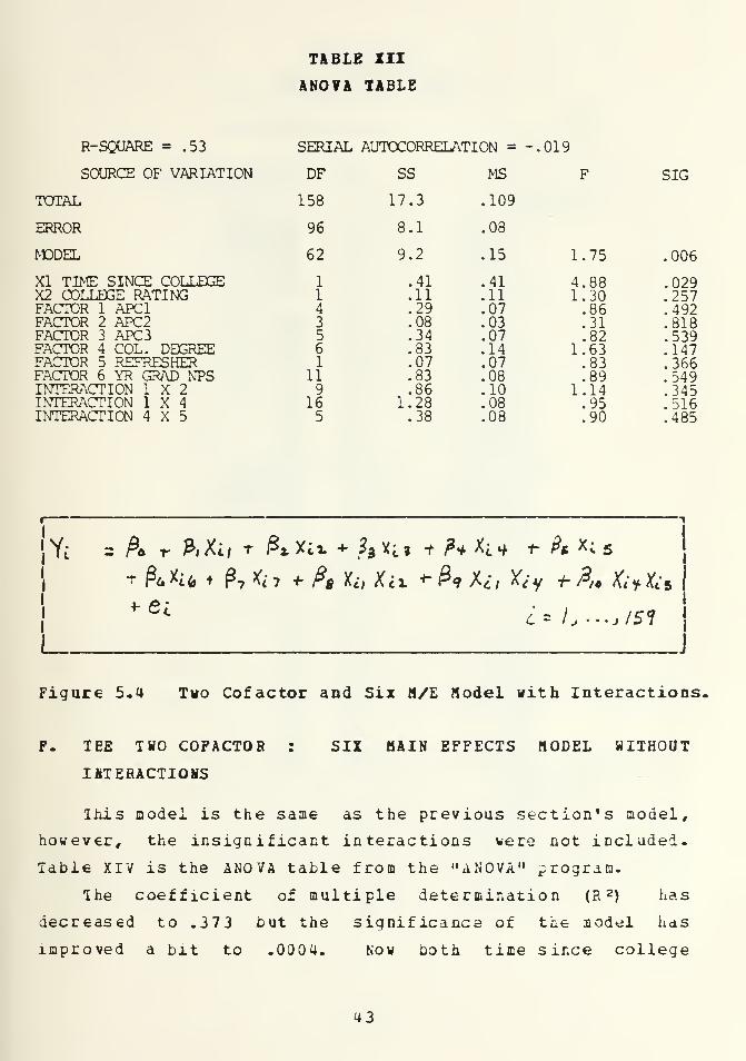
TABLE XII

ANOTA TABLE

R-SQUARE = .53

SOURCE OF VARIATION

TOTAL

ERROR

NDDEL

XI TIME SINCE COLLEGEX2 COLLEGE RATINGFACTOR 1 APC1FACTOR 2 APC2FACTOR 3 APC3FACTOR 4 COL. DEGREEFACTOR 5 REFRESHERFACTOR 6 YR GRAD NPSINTERACTION 1X2INTERACTION 1X4INTERACTION 4X5

SERIAL AUTOCORRELATION = -.019

DF

158

96

62

SS

17.3

8.1

9.2

MS

.109

.08

.15 1.75

SIG

.006

1 .41 .41 4.88 .0291 .11 .11 1.30 .2574 .29 .07 .86 .4923 .08 .03 .31 .8185 .34 .07 .82 .5396 .83 .14 1.63 .1471 .07 .07 .83 .366

11 .83 .08 .89 .5499 .86 .10 1.14 .345

16 1.28 .08 .95 .5165 .38 .08 .90 .485

f Mi* P7 *<7 + h X*, Xcl <-&vUi fty 4-?,. &>&

Figure 5.4 Tvo Cofactor and Six M/E flodel with Interactions.

TBE TWO COFACTOR

IBTERACTIOMS

SIX MAIN EFFECTS MODEL WITHOUT

Ihis model is the same as the previous section's model,

however, the insignificant interactions were not included.

Table XIV is the ANOVA table from the "ANOVA" program.

Ihe coefficient of multiple determination (R 2) has

decreased to .373 but the significance of tne model has

improved a bit to .0004. Now both time since college

43

TABLE XIII

BETA COEFFICIENTS

TERM

COVARIABLES

BETA COEFFICIENTS

X(l):X(2):

CONSTANT:MAIN EFFECTS

FACTOR (1):LEVEL(l)LEVEL(2LEVEL 3LEVEL(4LEVEL(5)

FACTOR (2):LEVEL(l)LEVEL 2LEVEL(3)LEVEL(4)

FACTOR (3):LEVEL (1LEVEL 2)LEVEL 3LEVEL 4LEVEL 5LEVEL(6)

FACTOR (4):LEVEL(l)LEVEL(2LEVEL (

3

LEVEL(4LEVEL 5LEVEL(6)LEVEL(7)

FACTOR (5):LEVEL(l)LEVEL(2)

FACTOR ( 6 )

:

LEVEL ( 1

)

LEVEL 2LEVEL(3)LEVEL(4LEVEL(5LEVEL(6)LEVEL(7LEVEL(8)LEVEL(9)LEVEL 10LEVEL(11

INTERACTIONSNUMBER ( 1 )

:

LEVELflLEVEL(2LEVEL (3LEVEL(4)LEVEL(5)LEVEL ( 6

)

LEVEL 7LEVEL(8)LEVELO)

.025 Time Since College

.073 College Rating3.642

APC1 APC Code: .203 APC0: -.068 APC1: -.134 APC2: -.142 APC3: .141 APC4

APC2: .038 APC0

.054 APC1: -.046 APC2: -.046 APC3

APC3: .019 APC0: -.010 APC1: -.060 APC2: .045 APC3: -.078 APC4

.084 APC5COLLEGE DEGREE

: .509 B'jsiness: -.029 Engineering: .259 Humaniries: -.017 Math

-.295 Social Science: -.340 Naval Science: .087 Operations Analysis

REFRESHER-.116 Refresher Yes.116 Refresner No

YEAR GRADUATED NFS133

-.115-.056.186.284

-.088.032

-.109.064

-.068-.042

19741975197619771978197919801981198219831984

APC1 X APC2 INTERACTIONS

.089

.213,032.447.275.125,073,341248

1X11 X 2XXXXX

3 X4 X

4U

TABLE XIII

BETA COEFFICIENTS (cont'd.)

NUMBER (2):

LEVEU1LEVEU2LEVEL(3LEVEL 4LEVEL(5LEVEL 6LEVEL(7LEVEL 8LEVEL 9LEVEL 10LEVELUlLEVEL(12LEVEL 13LEVEL(14)LEVEL 15LEVELU6

NUMBER (3):

LEVEL (1LEVEL (2LEVEL 3

LEVEL 4LEVEL(5

1.332 1 X 1

-.660 1 X 2-.688 1 X 3-.043 1 X 4

.472 1 X 5-.114 1 X 6.013 2 X 1

.377 2 X 3

.422 2 X 4

.067 2 X 5-.155 3 X 2-.085 3 X 3.156 3 X 6.113 4 X 1

.311 4 X 4

.340 4 X 5

4X5 INTERACTION

.192 1 X 1

.134 2 X 1-.591 3 X 1

.046 4 X 1

.025 5 X 1

(significance of .03) and APC 1 (significance of .005) are

seen to be very significant factors. This version of the

covariance model is simple with fewer terms and is snown in

Figure 5.5 .

Table XV is a listing of the beta coefticients provided

as an output from the "ANOVA" program. The levels of the

APC 1 variable are seen to contribute positively at the first

two levels and negatively at the lower three levels as one

would logically expect. The APC2 variable also "behaves" in

a similar fashion from level one through level four.

45

TABLE ZI7

AHOTA TABLE

R-SQUARE = .37

SOURCE OF VARIATION

TOTAL

ERROR

MODEL

XI TIME SINCE COLLEGEX2 COLLEGE RATINGFACTOR 1 APC1FACTOR 2 APC2FACTOR 3 APC3FACTOR 4 COL. DEGREEFACTOR 5 REFRESHERFACTOR 6 YR GRAD NPS

SERIAL AUTOCORRELATION = .017

DF

158

126

32

1

1

43561

11

SS

17.3

10.9

6.4

.41

.121.33.22.35.92.00.59

MS

.109

.09

.20

.41

.12

.33

.07,07,15,00,53

2.34

SIG

0004

4.79 .0301.43 .2343.86 .005.84 .475.81 .547

1.79 .106.01 .974.62 .801

r

P* v> A x*-i +^xa rfisKc 5 t pV X< y

*A X c-s f Pc Xu + fi*Xt'7 te $

c

L = K- ..,'**

Figure 5.5 Two C/F and Six H/E Model without Interactions.

G. THE FOOB COFACTOB AND TBEE2 SAIN EFFECTS HODEL WITH

IHTEfiACTIONS

The next model uses the variables time since college,

college rating, year graduated from NFS and length of

retresher as cofactors. It includes APC1, college degree

and designator as main effects. The model also evaluates

the interaction between APC1 and college degree. This

covanance model has a coefficient of multiple determination

46

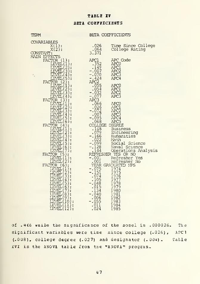
TABLE XV

BETA COEFFICIENTS

TERM

COVARIABLESX(lX(2

CONSTANT:MAIN EFFECTS

FACTOR (1)LEVEL (1LEVEL 2LEVEL 3LEVEL(4LEVEL(5)

FACTOR (2):LEVELd)LEVEL(2LEVEL 3levelU

FACTOR (3):LEVELdLEVEL 2LEVEL 3

LEVEL(4LEVEL(5LEVEL(6

FACTOR (4):LEVELdLEVEL(2LEVEL 3LEVEL(4LEVEL(5LEVEL(6LEVEL(7

FACTOR (5):LEVELd)LEVEL(2)

FACTOR (6):LEVELd)LEVEL 2LEVEL 3LEVEL 4LEVEL(5LEVEL(6LEVEL(7LEVELLEVELLEVELLEVEL(11LEVEL(12

BETA COEFFICIENTS

910

.026

.0643.371

APC1.352.149

-.007-.070-.424APC2.055.054

-.032-.077APC3.066.026

-.072.007

-.095.068

Time Since CollegeCollege Rating

APC CodeAPC0APC1APC2APC3APC4

APC0APC1APC2APC3

APC0APC1APC2APC3APC4APC5

COLLEGE DEGREE.148 Business.079 Enqineering

-.166 Humanities.022 Math

-.099 Social Science-.128 Naval Science.144 Operations Analysis

REFRESHER YES OR NO-.001 Refresher Yes.001 Refresher NoYEAR GRADUATED MPS

-.075 1974-.151 1975.074 1976.105 1977

-.048 1978.015 1979.134 1980

-.040 1981.006 1982

-.055 1983.011 1984.024 1985

of .466 wnile the significance of the model is .000026. The

significant variables were time since college (.026), A?C1

(.008), college degree (.027) and designator (.004). Table

XVI is the ANOVA table from tne "ANOVA" program.

47

TABLE I?I

ANOfA TABLE

R-SQUARE = .47

SOURCE OF VARIATION

TOTAL

ERROR

MODEL

XI TIME SINCE COLLEGEX2 COLLEGE RATINGX3 YR GRAD NPSX4 LENGTH OF REFRESHERFACTOR 1 APC1FACTOR 2 COLLEGE DEGREEFACTOR 3 DESIGNATORINTERACTION 1X2

SERIAL AUTOCORRELATION = -.004

DF

158

119

39

SS

17.3

9.3

8.1

MS

.109

.08

.21 2.66

SIG

00003

1 .39 .39 5.07 .0261 .15 .15 1.90 .1711 .03 .03 .37 .5451 .07 .07 .87 .3554 1.13 .28 3.65 .0086 1.16 .19 2.48 .0278 1.88 .23 3.02 .004

17 1.01 .06 .77 .730

Ccce again the interaction term does not appear to be

significant. The particular covariance model is shown in

Figure 5.6 .

Yt = fit+ff,**, rP7 *iz +P**i* tPyXi 9 rAX<T*-&*£* +07*1? T0tXi* tfifXtiXtz i <°l

Figure 5.6 4 Cofactor and 3 M/E Sodel with Interactions.

Table XVII is a listing of the beta coefficients from

the "ANGVA" program. It can be seen that the variaole

length of refresher contributes negatively to the overall

performance average. The APC1 variable performs logically

in decreasing order from the code to the lower APC1 code

of 4.

48

TABLE ZTII

BETA COEFFICIENTS

TERM

COVARIABLESX(lX(2X 3X(4

CONSTANT:MAIN EFFECTS

FACTOR (1):LEVEL(l)LEVEL(2LEVEL 3LEVEL 4LEVEL(5

FACTOR (2)LEVEL 1

LEVEL 2LEVEL(3LEVEL(4LEVEL(5LEVEL(6LEVEL(7

FACTOR (3):LEVEL(l)LEVEL(2LEVEL(3)LEVEL(4LEVEL 5LEVEL(6LEVEL(7LEVEL(8LEVEL(9

INTERACTIONSNUMBER ( 1 )

:

LEVEL (1LEVEL 2LEVEL(3)LEVEL(4LEVEL(5)LEVEL(6LEVEL 7LEVEL (8LEVEL(9LEVEL 10LEVEL 11LEVEL 12LEVELC13LEVEL(14LEVEL 15LEVEL(16LEVELU7

BETA COEFFICIENTS

.022 Time Since College

.076 College Rating

.005 Year Graduated NPS-.035 Length of Refresher3.231

APC1 APC Code.798 APC0.262 APC1.024 APC2

-.063 APC3-1.021 APC4COLLEGE DEGREE

. 376 Business

.138 Engineering-.194 Humanities.016 Math

-.246 Social Science-.251 Naval Science.161 Operations Analysis

DESIGNATOR-.177-.041.217.117.117.082.056.183

-.554

110011101120131013201400161031001130

APC1 X APC2 INTERACTION

-.926-.422-.385.076

-.437-.148.014

2.146.300

-.152-.350-.030.020.122.148.310.334

1 X

X 1

H. STUDY. HODEL :THfiEE MAIN EFFECTS :FOOR COFACTORS :NO

INTERACTIONS

The interaction between the variables APC 1 and college

degree was removed and the resulting model is tne one

49

selected as the study model. cnce again the four cofactors

are time since college, college rating, year graduated from

NPS and length of refresher. The main effects are the first

academic profile code (APC1), college degree and designator.

The model is seen in Figure 5- 7 .

Y- ^Porfrtci+Pxlix *%Ks +t*Xi* *0s K;s

(I -- Ij • •, /*7

I

Figure 5.7 4 Cofactor and 3 fi/E Hodel without Interactions.

Table XVIII is the ANOVA table from the "ANOVA" program.

The coefficient of multiple determination is .408 and the

model nas an extremely high significance of .00000007. This

model shows the significance of time since college (.015),

APC1 (.00002), college degree (.032) and designator (.034)

to all be important factors in explaining the variability in

fourth quarter qpr's of students in tne OA curriculum.

labxe XIX is a listing of the beta coefficients from the

"ANOVA" program. The cofactors time since college, college

rating and year graduated from NPS have a positive contribu-

tion to the fourth guarter gpr while length of refresher

contributes negatively. APC 1 nenaves in a very logical

fashion. The better one's college performance reflects a

more positive contribution to the dependent variable (fourth

quarter gpr) . This same variable contributes in a negative

manner as the college qpr decreases to the lower two levels.

The college majors of business, engineering, math and opera-

tions analysis all have a positive beta coefficient while

the social science, humanities and naval science majors have

50

TABLE I 711

I

AHO¥A TABLE

R-SQUARE = .41 SERIAL AUTOCORRELATION = .057

SOURCE OF VARIATION DF SS MS F SIG

TOTAL 158 17.3 .110

ERROR 136 10.3 .08

MODEL 22 7.1 .32 4.25 .00000007

XI TIME SINCE COLLEGEX2 COLLEGE RATINGX3 YR GRAD NPSX4 LENGTH OF REFRESHERFACTOR 1 APC1FACTOR 2 COLLEGE DEGREEFACTOR 3 DESIGNATOR

11

1

1

468

.46

.20

.02

.082.241.081.79

.46

.20

.02

.08

.56

.18

.22

6.132.71.30

1.097.432.392.96

.015

.102

.583

.298

.000

.031

.004

negative coefficients. In this model, all designators

except for 1100,1110 and 1130 have a positive beta coeffi-

cient. Although this model did not have the highest coeffi-

cient of multiple determination, it is a straightforward,

significant model.

51

TABLE XII

BETA COEFFICIENTS

TERM

COVARIABLESX(lX(2X(3X(4

CONSTANT:MAIN EFFECTS

FACTOR (1):LEVEL(l)LEVEL 2LEVEL(3)LEVEL(4LEVEU5)

FACTOR (2):LEVEL(l)LEVEL(2)LEVEL(3LEVEL (4LEVEL 5)LEVEL (6LEVEL(7

FACTOR (3):LEVELdLEVEL(2LEVEL(3LEVEL(4LEVEL(5LEVEL(6LEVEL 7LEVEL (8LEVELO)

BETA COEFFICIENTS

.023 Time since college

.083 Colleae Rating

.004 Year Graduated NPS-.037 Length of Refresher3.265

APC1.351 APC0.195 APC1.001 APC2

-.114 APC3-.433 APC4COLLEGE DEGREE.061 Business.138 Engineering

-.175 Humanities.033 Math

-.097 Social Science-.101 Naval Science.141 Operations Analysis

DESIGNATOR-.091-.045.218.100.117.072.030.148

-.549

110011101120131013201400161031001130

52

VI. COfCIOSIOHS AND EECOMMENDATIONS

A. CCICIUSIOHS

The study shows some interesting insights into evalu-

ating future performance in regards to the Operations

Analysis curriculum. It would initially seem guite logical

to assume that the longer an individual has been out of

college the harder it would be for him or her to return and

succeed in the academic environment. However, this does not

appear to be the case as reflected by this study. In

searching for an explanation, motivation could play a major

role. Those students who start a curriculum middle to late

in their military service, have most likely decided to make

the service a career. They are likely to realize how impor-

tant successful completion of their chosen subspecialty is

to their remaining time in the service and are conseguently

willing and ready to make whatever effort is reguired to

accomplish that goal. More correctly, they are out to do

the best they can possibly dc while earning their degree.

This grouping would also imply that they are most probably

of an age to have their families and a maturity to be able

to concentrate their efforts toward a long term goal.

In almost every model tested, the variable for college

academic performance (APC1) was seen to be a significant

factor- Surprisingly, the math (APC2) and technical code

(APC3) did not prove to be very meaningful in the manner of

explaining the variability of student performance. Given a

choice it appears to be more logical to select a student

based on his performance in his chosen field rather than to

strictly choose based on his undergraduate degree.

53

The negative contribution of length of refresher prob-

ably means those individuals who need it most are in fact

getting the extra guarter or two. This is possibly

confounded by the ability to get an extra quarter or two

"after the fact", in that, early poor performance can "flag"

a student and draw attention to him. With liasion between

the curricular officer and the student's detailor, an addi-

tional guarter or two can get added to his tour at NPS.

With the possible exception of business majors, there

are nc surprises in the college degree variable. Those

students with college majors of math, engineering, opera-

tions analysis and business in fact nave performed as an

average better than the humanities and social science

ma j ors.

The designator variable was in fact significant to the

model and showed the designators 1100, 1110 and 1130 to have

a negative contribution toward fourth guarter academic

performance.

The study population covered only those students who

successfully completed the GA curriculum. Of course one

would want to infer that the insights gained from the study

group would apply to the target group of future OA students.

This can not be done in the strict predictive sense but the

study can suggest that any selection of future OA students

be influenced by these results.

The model preferred by the author is discussed in

section H of Chapter V. This model has an R 2 value of .4 1

while another model investigated (section E of Chapter V)

attains an R 2 of .5 3. The model of section H has a much

higher level of significance and is a simpler less complex

model.

54

B. RECOHHEMDATIOHS

A very interesting study to complement this one would be

to investigate those Navy students who started but did not

complete the OA curriculum during the last ten years. The

study group would not be very large but it could possibly

provide additional insight into the problem.

Recent interest has been generated to have all NPS

students take the Graduate Record Examination (GRE)

-

Currently, this predictor is available for very few individ-

uals in this study. Exactly when the test will be taken is

still to be determined but a study combining academic

profile codes and the GRE could prove to be much more

successful in developing a predictive model. In this

regard, the recommendation that the APC's and GRE scores be

maintained by NPS as a permanent part of the student's tran-

script is a necessity for future studies of this type.

Another study of interest would be to determine the

validity and usefulness of the newly established Technical

Transition Program. This new program will reguire a few

years before the data can be collected studied but adequate

records must be maintained in order to evaluate it in the

future.

55

APPENDIX A

ACRONYMS AND ABBREVIATIONS

APC Academic Profile Code

APCl Academic Profile Code 1st Digit

APC2 Academic Profile Code 2nd Digit

APC3 Academic Profile Code 3rd Digit

ARE Academic Record Evaluation

GRE Graduate Record Examination

NMPC Naval Military Personnel Command

NPS Naval Postgraduate School

OA Operations Analysis

QPR Quality Point Rating

r Pearson's Product Moment Correlation Coefficient

R^ Coefficient of Multiple Determination

TTP Technical Transition Program

APPENDIX B

ACAOEMIC RECORD EVALUATION Year GroupNPS 50*0/2 (12-81)

w '-• KAMI M.lf

COLLEGE 1 Undergraduate/Graduate} DEGREE MAJOR DATE

KUKI COO* 17 PC '• total aro :o-a 34.30 CUUITlNOIKfl 10O4

ACAOEMIC PROFILE CODE GRE SCORES GMAT SCORESQPR MKkTH TECH V Q OATS T V Q OATE

la a 40 43-44 40-4)1 U-M 1T-W 40-4I 43-44

ABSTRACT FROM TRANSCRIPT

SU8JECT AREANUMBER OF GRAOES IN EACH SUBJECT AREA

A 3 C f w

MATH - PRE-CALCULUS

M •7 M 4* 70 71

CALCULUSn 74 7S 7* " '•

uao mo. a

POST CALCULUS17 1* 1* 30 31 3]

COMPUTERS. NUMERICAL ANALYSIS34 I* It 37 2* 3*

STATISTICS

J1 13 13 14 331 30

PHYSICS - LOWER DIVISIONm n ad 41 43

i43

UPPER DIVISION

41 44) 47 44) 44) 1 M

CHEMISTRYu S3 M M M 57

OTHER PHYSICAL SCIENCE*

m •0 41 1 43 43 44

AERONAUTICAL/MECHANICAL ENGINEERINGm 47 M 40 i

70 1 71

ELECTRICAL ENGINEERINGn\ 74 75 7« 77 '•

GfcMO NO. J

OTHER ENGINEERING17 If IS 20

!

ACCOUNTING

1

24 39 I :•1

37 2* 1 .1

!

ECONOMICS

BUSINESS AOMIN/MANAGEMENT

HISTORY

GOVERNMENT/INTERNATIONAL RELATIONS

'Metenmlogy. Oceanography. Geology

57

APPENDIX C

THE STUDY DATA

Column

1 Index

2 APC1

3 APC2

4 APC3

5 4th QTR QPR

6 6th QTR QRAD QPR

7 8th QTR Total GRAD QPR

8 8th QTR Total QPR

9 College Rating — Main Effect

10 College Degree

3 = Business6 = Engineering7 = Humanities8 = Math9 = Social Science

10 = Naval Science11 = OA

11 Designator

1 = 110X2 = 111X3 = 112X4 = 131X5 = 132X6 = 140X7 = 161X8 = 310X9 = 113X

12 Time since college (in months)

13 Refresher (1 = yes, 2 = no)

14 College Rating (cofactor)

15 Year graduated from NPS

16 A selection value

17 Length of Refresher (in quarters)

18 Time since college (main effect)

58

1 2 2 2 3.07 3.15 3.25 3.20 5 10 1 62 1 4.36 74 1 .5 3

2 1 2 3.43 3.21 3.25 3.40 5 10 2 55 1 4.36 74 1 1 2

3 2 2 3.29 3.22 3.26 3.33 4 8 6 61 1 3.96 74 1 .5 3

4 2 2 3.43 3.24 3.32 3.45 5 8 4 63 1 4.36 74 1 2 3

5 2 2 3 3.11 3.03 3.06 3.03 5 10 8 57 1 4.36 74 1 .5 2

6 4 2 4 3.11 3.08 3.26 3.24 6 6 5 39 1 4.56 74 1 2 2

7 2 1 3.04 3.17 3.22 3.15 6 6 2 52 2 4.70 74 1 2

8 3 2" 3 2.63 2.83 3.08 2.98 5 10 8 63 1 4.36 74 1 .5 3

9 3 2 3 2.85 3.19 3.30 3.22 5 10 2 57 1 4.36 75 1 2 2

10 2 3 3.17 3.08 3.13 3.22 6 8 2 58 1 4.69 75 1 1 2

11 2 2 3 3.16 3.21 3.35 3.29 2 9 5 63 2 2.76 75 1 3

12 3 2 4 2.99 3.18 3.27 3.16 5 10 8 135 1 4.36 75 1 .5 6

13 2 1 2 3.07 3.08 3.17 3.16 3 3 3 50 1 3.12 75 1 2 2

14 2 1 3 3.09 3.03 3.13 3.18 5 9 2 60 1 4.06 75 1 2 2

15 2 3 4 2.97 3.06 3.13 3.07 5 3 4 75 1 4.21 75 1 2 3

16 1 3 3.89 3.83 3.78 3.80 5 8 8 58 2 4.36 75 1 2

17 2 3 3.31 3.36 3.39 3.37 3 3 4 87 1 3.03 75 1 2 4

18 2 1 2 3.02 3.00 3.16 3.20 5 6 2 75 1 4.4 75 1 .5 3

19 2 2 2 3.35 3.28 3.28 3.35 5 8 4 58 1 4.01 75 1 .5 2

20 1 3 3.32 3.33 3.50 3.48 3 8 2 46 1 3.49 75 1 2 2

21 4 2 3 3.02 3.04 3.08 3.06 6 6 4 165 1 4.91 76 1 .5 6

22 4 1 3.50 3.41 3.40 3.40 5 11 4 58 1 4.36 76 1 2 2

23 1 3.59 3.47 3.44 3.53 4 6 4 82 1 3.96 76 1 .5 3

24 3 2 3 3.08 3.28 3.36 3.36 5 10 4 81 2 4.36 76 1 3

25 2 2 2 3.76 3.76 3.77 3.77 5 11 2 34 1 4.36 76 1 .5 1

26 2 2 3 3.49 3.49 3.55 3.57 5 11 2 39 2 4.36 76 1 2

27 2 1 3.58 3.67 3.64 3.62 5 6 5 74 2 4.21 76 1 3

28 2 2 3 3.61 3.08 3.41 3.43 6 3 4 57 2 4.54 77 1 2

29 2 2 3 3.45 3.42 3.51 3.52 5 9 4 87 2 4.36 77 1 4

30 2 2 1 3.79 3.72 3.74 3.79 5 6 5 51 2 4.36 77 1 2

31 2 2 3 3.34 3.20 3.07 3.21 5 3 2 58 2 4.36 77 1 2

32 1 1 1 3.67 3.52 3.60 3.63 5 8 5 75 2 4.36 77 1 3

33 3 2 1 3.21 3.05 3.25 3.17 6 6 4 47 2 4.57 77 1 2

59

34 3 3 2 3.22 3.14 3.27 3.31 5 10 4 82 1 4.36 77 1 2 3

35 3 5 3.43 3.40 3.41 3.41 3 3 4 23 2 3.29 78 1 1

36 2 1 2 3.60 3.63 3.66 3.64 5 8 2 111 1 4.36 78 1 .5 5

37 3 3 4 3.97 3.98 3.98 3.99 6 3 4 85 1 4.69 79 1 1 4

38 2 3 4 3.91 3.85 3.93 3.89 4 8 3 75 2 3.94 79 1 3

39 2 2 1 2.93 3.21 3.32 3.19 3 8 2 46 2 3.15 79 1 2

40 3 2 4 3.45 3.41 3.48 3.41 5 11 4 63 1 4.36 79 1 2 3

41 2 1 2 3.66 3.71 3.69 3.68 5 10 2 129 2 4.36 79 1 5

42 2 2 3 2.94 3.24 3.27 3.23 5 6 5 52 2 4.17 79 1 2

43 2 Z 3 3.53 3.49 3.53 3.56 5 11 4 58 2 4.36 79 1 2

44 3 2 1 3.32 3.34 3.40 3.40 5 6 4 123 2 4.4 79 1 5

45 3 2 3 3.03 3.21 3.33 3.21 5 9 4 123 1 4.36 79 1 .5 5

46 3 3 4 2.78 2.95 3.04 3.01 5 11 2 46 1 4.36 79 1 2 2

47 2 3 4 3.37 3.39 3.37 3.36 5 8 4 70 1 4.12 79 1 2 3

48 3 2 3 3.37 3.23 3.31 3.36 6 8 8 144 1 4.54 79 1 .5 6

49 2 2 3 3.36 3.57 3.60 3.48 5 8 3 99 2 4.36 79 1 4

50 2 2 3 3.30 3.49 3.53 3.48 5 11 5 87 2 4.36 79 1 4

51 2 3 3 3.58 3.68 3.71 3.65 6 6 2 97 1 4.73 80 1 2 4

52 3 2 3 3.69 3.58 3.56 3.57 5 8 4 109 1 4.36 80 1 1 5

53 1 2 3.85 3.83 3.85 3.84 5 11 5 51 2 4.36 80 1 2

54 3 2 3 3.73 3.63 3.68 3.71 6 8 8 108 2 4.54 80 1 4

55 2 2 1 3.64 3.74 3.77 3.73 5 10 4 87 2 4.36 80 1 4

56 1 1 3.77 3.80 3.84 3.85 6 6 8 111 2 4.69 80 1 5

57 2 1 3 3.12 3.31 3.30 3.19 6 8 2 59 2 4.59 80 1 2

58 2 2 3 3.42 3.44 3.57 3.52 5 6 8 88 2 4.39 80 1 4

59 1 4 3.76 3.77 3.77 3.77 2 8 8 83 2 2.77 80 1 3

60 1 2 5 3.73 3.82 3.83 3.81 3 9 8 59 1 3.10 81 1 1 2

61 3 2 2 3.14 3.14 3.32 3.25 5 11 2 51 2 4.36 81 1 2

62 2 1 1 3.84 3.82 3.85 3.86 6 9 8 111 2 4.83 81 1 5

63 3 3 4 3.48 3.59 3.57 3.51 3 3 4 124 1 3.11 81 1 2 5

64 2 2 3 3.15 3.39 3.40 3.27 5 8 2 46 2 4.36 81 1 2

65 2 4 3.13 3.43 3.41 3.30 4 8 8 117 2 3.70 81 1 5

66 3 2 3 3.22 3.25 3.36 3.32 5 6 2 87 1 4.4 81 1 .5 4

67 3 1 2 3.10 3.23 3.32 3.23 4 8 7 100 2 3.90 81 1 4

60

68 3 3 4 3.03 3.11 3.26 3.19 5 11 4 66 1 4.36 81 1 2 3

69 1 2 4 3.46 3.64 3.71 3.62 5 11 5 58 2 4.36 81 1 2

70 2 2 4 2.93 3.22 3.25 3.09 5 7 4 94 1 4.36 81 1 .5 4

71 2 3.97 3.95 3.94 3.94 5 8 3 51 2 4.36 82 1 2

72 3 3 5 3.12 3.24 3.24 3.18 4 7 4 147 1 3.52 82 1 2 6

73 4 2 4 2.43 2.90 3.02 2.77 5 11 2 45 2 4.36 82 1 2

74 3 3 4 3.76 3.72 3.73 3.75 5 6 2 109 1 4.38 82 1 2 5

75 2 2 3 3.87 3.84 3.83 3.82 6 6 7 63 2 4.76 82 1 3

76 2 1 3 3.83 3.88 3.89 3.87 6 8 8 88 2 4.88 82 1 4

77 1 0' 3 3.36 3.53 3.52 3.44 5 8 2 47 2 4.06 82 1 2

78 1 1 1 3.67 3.69 3.75 3.75 6 6 8 69 1 4.57 82 1 .5 3

79 1 1 5 3.59 3.64 3.72 3.71 6 3 8 111 2 4.63 82 1 5

80 1 2 2 3.28 3.47 3.49 3.44 4 8 2 47 1 3.95 82 1 .5 2

81 2 3 3.56 3.62 3.64 3.63 5 8 5 64 1 4.17 82 1 .5 3

82 2 3 4 3.40 3.42 3.42 3.38 6 3 5 123 1 4.6 82 1 2 5

83 1 2 3.27 3.33 3.37 3.36 2 8 5 70 1 2.37 82 1 .5 3

84 2 1 3 2.90 3.06 3.15 3.06 4 8 2 71 1 3.90 82 1 .5 3

85 2 2 5 3.64 3.61 3.60 3.61 6 8 5 88 1 4.59 82 1 .5 4

86 2 2 3 3.65 3.58 3.60 3.66 4 8 1 71 1 3.72 83 1 .5 3

87 3 2 3 3.25 3.40 3.43 3.40 5 8 4 58 1 4.36 83 1 .5 2

88 1 4 3.39 3.33 3.38 3.42 4 11 7 75 2 3.97 83 1 3

89 3 3 1 3.39 3.52 3.52 3.48 6 6 4 70 1 4.54 83 1 2 3

90 1 1 5 3.83 3.82 3.79 3.81 6 7 5 104 1 4.93 83 1 .5 4

91 2 1 3 3.15 3.05 3.15 3.20 5 8 2 57 1 4.06 83 1 1 2

92 1 1 3 3.43 3.56 3.60 3.56 4 9 2 46 1 3.7 83 1 .5 2

93 2 2 1 2.97 3.09 3.25 3.20 5 6 2 45 2 4.01 83 1 2

94 1 2 3.75 3.67 3.70 3.73 4 8 5 183 1 3.53 83 1 .5 6

95 1 3.96 3.96 3.95 3.96 5 6 3 63 2 4.36 83 1 3

96 3 3.99 3.95 3.90 3.90 5 8 3 63 2 4.36 83 1 3

97 1 1 5 3.46 3.41 3.40 3.44 3 8 5 76 1 3.35 83 1 2 3

98 2 2 4 2.89 3.00 3.15 3.08 5 9 2 51 1 4.36 83 1 .5 2

99 3 3 4 2.77 2.94 3.07 3.09 4 8 5 86 1 3.93 83 1 2 4

100 3 4 3.59 3.67 3.63 3.60 3 9 1 93 1 3.49 83 1 .5 4

101 3 3 3 3.32 3.32 3.31 3.31 5 11 4 118 1 4.36 83 1 .5 5

61

102 2 2 3 3.30 3.35 3.43 3.43 6 9 4 147 1 4.9 83 1 .5 6

103 3 2 4 3.30 3.10 3.21 3.33 5 11 2 51 1 4.36 83 1 .5 2

104 1 2 3 3.97 3.97 3.96 3.97 6 3 8 106 1 4.85 83 1 .5 4

105 2 1 3 3.70 3.62 3.67 3.72 5 8 2 142 1 4.36 83 1 .5 6

106 2 1 3 3.51 3.46 3.53 3.56 5 11 4 63 2 4.36 83 1 3

107 1 3 4 2.62 2.86 3.13 3.09 6 9 9 99 1 4.63 83 1 2 4

108 2 2 1 3.82 3.85 3.86 3.86 6 6 3 135 1 4.9 83 1 .5 6

109 2 3 4 3.19 3.22 3.29 3.31 3 8 2 63 1 3.38 83 1 2 3

110 2 3.34 3.18 3.33 3.39 4 8 1 171 1 3.93 83 1 1 6

111 3 2 4 3.06 3.22 3.27 3.25 3 9 5 63 2 3.21 83 1 3

112 3 3 3 3.07 3.16 3.28 3.23 5 6 2 123 1 4.36 83 1 .5 5

113 2 2 1 3.05 3.27 3.33 3.25 6 8 2 105 2 4.86 83 1 4

114 3 2 2 3.08 3.04 3.14 3.19 5 6 2 135 1 4.36 83 1 .5 6

115 2 1 2 3.82 3.77 3.74 3.77 5 11 3 63 1 4.36 83 1 .5 3

116 2 2 4 3.41 3.39 3.45 3.49 5 6 2 45 2 4.03 83 1 2

117 3 2 3 3.82 3.77 3.74 3.79 3 8 5 130 2 3.13 84 1 5

118 2 2 2 2.95 3.15 3.20 3.13 5 8 2 45 2 4.36 84 1 2

119 2 2 3 3.34 3.39 3.46 3.50 5 6 2 45 2 4.36 84 1 2

120 2 3 3.44 3.45 3.45 3.47 5 8 4 57 1 4.36 84 1 .5 2

121 2 2 4 3.32 3.43 3.47 3.46 6 9 2 45 1 4.81 84 1 .5 2

122 2 3 5 3.11 3.18 3.23 3.20 5 7 4 70 1 4.14 84 1 2 3

123 2 3 2 3.07 3.13 3.15 3.13 6 3 4 59 1 4.69 84 1 2 2

124 3 3 4 2.96 3.02 3.11 3.09 3 8 4 95 1 3.06 84 1 2 4

125 1 2 4 3.47 3.53 3.54 3.54 5 3 4 58 1 4.12 84 1 .5 2

126 2 2 3 3.17 3.25 3.31 3.32 6 8 2 47 2 4.6 84 1 2

127 1 2 5 3.35 2.84 2.95 3.10 5 9 3 82 2 4.14 84 1 3

128 2 2 3 3.81 3.86 3.87 3.86 6 8 2 47 2 4.55 84 1 2

129 2 3 3 3.38 3.54 3.54 3.48 5 8 4 107 1 4.11 84 1 .5 4

130 3 3 3 3.81 3.76 3.54 3.48 5 11 2 118 1 4.36 84 1 .5 5

131 2 2 3 3.14 3.22 3.30 3.27 4 6 9 112 1 3.95 84 1 .5 5

132 3 2 2 3.14 3.04 3.13 3.19 5 6 2 50 2 4.36 84 1 2

133 2 3 5 3.00 3.08 3.12 3.12 3 9 5 114 1 3.17 84 1 2 5

134 3 3 3 3.79 3.76 3.79 3.82 5 6 4 164 1 4.4 84 1 2 6

135 1 4 3.25 3.02 3.07 3.16 4 8 8 93 1 3.9 84 1 .5 4

62

136 4 3 4 3.15 3.17 3.22 3.22 5 11 4 111 1 4.36 84 1 2 5

137 3 2 4 3.79 3.62 3.66 3.72 5 6 2 52 2 4.28 84 1 2

138 2 2 1 2.98 2.96 2.99 2.99 4 8 2 52 2 3.9 84 1 2

139 3 2 3 3.27 3.28 3.35 3.34 5 10 4 159 1 4.36 84 1 .5 6

140 2 1 4 3.42 3.33 3.36 3.39 5 11 5 63 1 4.36 84 1 .5 3

141 2 1 5 3.29 3.23 3.25 3.28 3 8 3 40 2 3.06 84 1 2

142 2 2 1 3.38 3.40 3.43 3.40 4 8 4 88 2 3.9 84 1 4

143 1 1 3 3.69 3.24 3.67 3.71 3 8 8 100 1 3.5 84 1 .5 4

144 2 3 4 3.84 3.81 3.83 3.82 5 3 8 151 1 4.4 85 1 1 6

145 2 I 3 3.35 3.41 3.46 3.45 5 8 2 46 1 4.36 85 1 .5 2

146 1 5 3.82 3.80 3.77 3.78 3 11 2 71 2 3.46 85 1 3

147 2 2 4 3.26 3.30 3.36 3.36 5 11 5 58 1 4.36 85 1 .5 2

148 2 2 4 2.83 3.01 3.10 3.05 5 9 2 46 1 4.36 85 1 .5 2

149 1 3 3.63 3.69 3.72 3.69 3 8 1 47 2 3.5 85 1 2

150 2 3 4 2.83 3.03 3.16 3.13 6 8 1 107 1 4.74 85 1 .5 4

151 2 2 3 3.59 3.63 3.63 3.63 6 8 5 58 1 4.71 85 1 .5 2

152 1 1 2 3.43 3.43 3.48 3.50 5 8 5 58 1 4.36 85 1 .5 2

153 3 2 3 3.30 3.29 3.38 3.39 5 10 2 178 1 4.36 85 1 .5 6

154 2 2 4 2.74 2.99 3.10 3.04 6 8 2 71 1 4.69 85 1 .5 3

155 3 2 4 3.27 3.28 3.33 3.35 5 11 2 58 2 4.36 85 1 2

156 2 2 1 3.85 3.82 3.82 3.85 6 8 8 142 2 4.9 85 1 6

157 2 2 1 3.98 3.93 3.92 3.93 5 6 5 64 1 4.06 85 1 .5 3

158 1 5 3.83 3.77 3.76 3.79 3 8 5 59 1 3.46 85 1 .5 2

159 3 2 1 3.46 3.48 3.55 3.56 5 6 4 94 1 4.36 85 1 .5 4

63

APPENDIX D

ADDIIIOHAL PRELIMINARY ANALYSIS

a:a. <o

o HQ<a:

O

t—O

>

r- k->

<o

O

Ifx

)

(

:

1

-y

»

N_ «

L-r •

-

» \v

A \"

*

.

U*-1

)lt

-

? 1 1

2

APC1

BOX-

• UtMfi• UtCMMSXAJ A.• outllOT

(m»o"«

CATEG. NO.PTS %-PTS Y-MEAN Y-DVN 25 50 .75

ALL CODES 159 1 3.398 0.2883 3.18 3.39 3.638 0.050314 3.7038 0.26711 3.4 3.69 3.95

1 28 0.1761 3.5107 0.28636 3.33 3.53 3.772 79 0.49686 3.3857 0.26924 3.17 3.39 3.623 39 0.24528 3.3149 0.26347 3.14 3.25 3.524 5 0.031447 3.12 0.16912 3.04 3.08 3.17

figure D. 1 6th Qtr Grad QPR vs APC1-

64

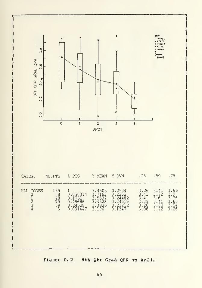
05

a:a.o <o

Q3OULt—ox00

f I

- f

•I i

-::

- •

N-

„

-

1

! :

- >

>

;

1 »

:

1

;

1

J1

•

BOX'

• UCMIS« UCDIMft

«W VI.

• eutiWfi

•

2

APC1

CATEG. NO.PTS %-PTS Y-MEAN Y-DVN 25 50 .75

ALL CODES 159 1 3.4503 0.2524 3.26 3.41 3.668 0.050314 3.7163 0.2255 3.41 3.72 3.9

1 28 0.1761 3.5632 0.24482 3.4 3.6 3.762 79 0.49686 3.4328 0.24519 3.25 3.41 3.633 39 0.24528 3.3826 0.21212 3.26 3.33 3.544 5 0.031447 3.196 0.1347 3.08 3.22 3.26

Figure D. 2 8th Qtr Grad QPfi vs APC1,

65

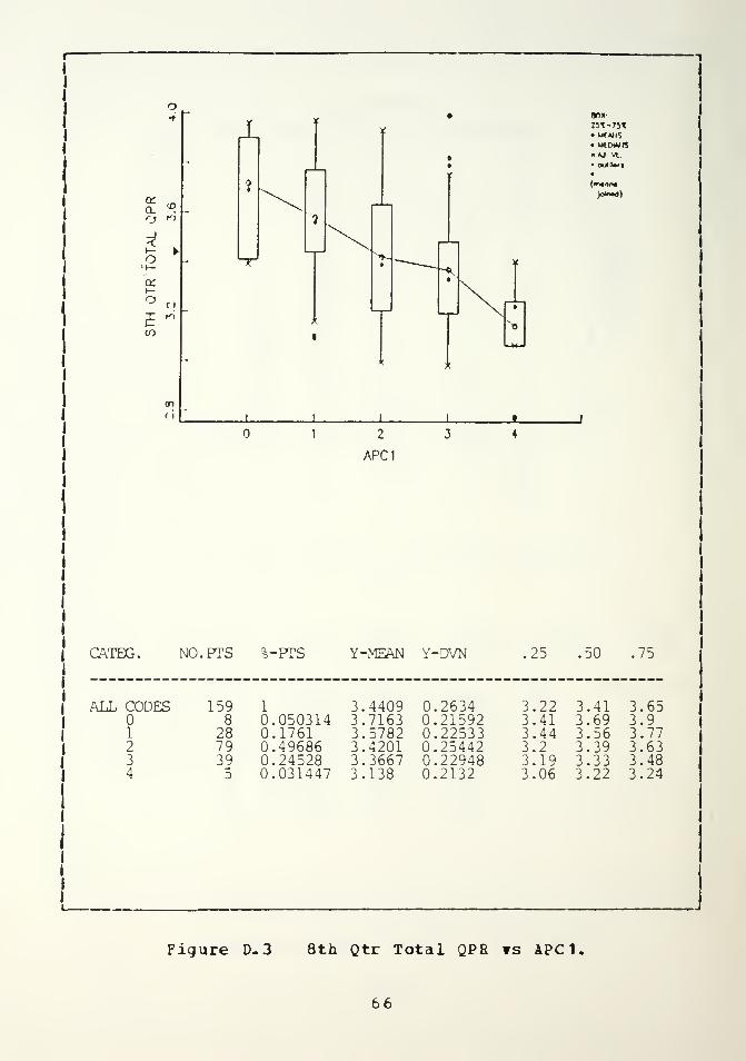
a. ">

& '

h-

I—

CO

I

:

)

4

:

i

-

?

•

<

- s

3 .

- J ^

.

3 :

;

l-*

<

>

* k

iiit*i

BOX-

23T-73X• ufwiS

• utrwrs«AJ vi

•

Pm4)

2

APC1

CATEG. NO.PTS 5-FTS Y-MEAN Y-DVN 25 .50 .75

ALL CODES 159 1 3.4409 0.2634 3.22 3.41 3.658 0.050314 3.7163 0.21592 3.41 3.69 3.9

1 28 0.1761 3.5782 0.22533 3.44 3.56 3.772 79 0.49686 3.4201 0.25442 3.2 3.39 3.633 39 0.24528 3.3667 0.22948 3.19 3.33 3.484 5 0.031447 3.138 0.2132 3.06 3.22 3.24

Figure D- 3 8th Qtr Total QPE vs APC1.

66

BOX:

• UEAM>• UEDUNS«XJ VI.

• Oulli«r«

•

CATEG. NO.PTS %-PTS Y-MEAN Y-DVN 25 50 75

ALL CODES 159 1 3.398 0.2883 3.18 3.39 3.6324 0.15094 3.4742 0.27154 3.22 3.43 3.67

1 29 0.18239 3.49 0.28439 3.24 3.52 3.712 76 0.47799 3.3551 0.27236 3.15 3.29 3.533 30 0.18868 3.3567 0.31022 3.11 3.24 3.67

Figure D. 4 6th Qtr Grad QPB ts APC2-

o7

cr>

a.o <o

Q "

b -

Xt—00

f i

^1

25X-7JT• ur »>',

• U(01M<S« «J A.• outiWii

•

(mtont

J L

1 2

APC2

CATEG. NO.PTS -PTS Y-MEAN Y-DVN 25 50 ,75

ALL CODES

1

23

15924297630

0.150940.182390.477990.18868

4503497554454195

3.3993

0.25240.23840.254650.237940.26589

3.263.32

3226

3.16

3.413.443.63.383.29

3.663.73.743.563.57

Figure D. 5 8th Qtr Grad QPR vs APC2.

b8

a ^

a:t—o

oox-

251-731• ueak;• UtWAN?» AJ W.

•

(m»o«l(oW.d)

APC2

CATEG. NO.PTS %-FTS Y-MEAN Y-DVN 25 50 75

ALL CODES 159 1 3.4409 0.2634 3.22 3.41 3.6524 0.15094 3.5179 0.22493 3.36 3.45 3.73

1 29 0.18239 3.5462 0.26059 3.28 3.63 3.752 76 0.47799 3.4017 0.2557 3.21 3.36 3.563 30 0.18868 3.3767 0.26924 3.13 3.31 3.51

Figure D.6 8th Qtr Total QPB vs APC2-

69

APC3

CATEG. 1 NO PTS lo/o-pTS 1 Y-MEAN | Y-DVN I .25 1 50 1 75

ALL 159 1 3.398 0.2883 3.18 3.39 3.634 0.025157 3.66 0.22814 3.41 3.47 3.8

1 19 0. 1 195 3 4868 0.29243 3.21 3.52 3.742 25 0.15723 3.3512 0.28053 3.14 3.23 3.633 59 0.37107 3.4203 25973 3.23 3 4 3 624 39 0.24528 3.3069 0.29217 3 03 3.28 3.53

13 0.081761 3.4492 0.30871 3.23 3.41 3.77

Figure D- 7 6th Qtr Grad QPfi vs APC3-

70

CATEG. 1 ho.pts |o/o-PTS I Y-MEAM | Y-DVN | .25 1 .50 1 .75

ALL 159 1 3.4503 0.2524 3.26 3.41 3.66

4 0.025157 3.6575 0.24108 3.4 3.44 3.84

1 19 0.1195 3.5374 0.25849 3.32 3.55 3.77

2 25 0.15723 3.4096 0.24289 3.25 3.32 3.66

3 59 0.37107 3 4737 0.2243 3.31 3.46 3.63

4 39 0.24528 3.3715 0.25334 3.15 3.33 3.54

13 0.081761 3.4669 0.28361 3.24 3.41 3.76

Figure D- 8 6th Qtr Grad QPR vs APC3-

71

a:

<oh-

\-

O

2 3

APC3

*f

-

I

9

.

: (

¥

to \^1')

* ^ j ,*<

^r'n»o

>

Tc

1

on

( I lilt, 1 1

BOX-

• UfA/IS

• UtOWIS>«J VI

• OUtlU'l

•

(fn*/mt

CATEG. I fJO.PTS lo/o-PTSI Y-MEAN | Y-DVN | . 25 I . 50 I .75

ALL 159 1 3 4409 0.2G34 3.22 3.41 3.65

4 0.025157 3.605 0.22809 3.4 3.53 3.85

19 0. 1195 3 5163 0.28621 3.2 3.56 3.79

25 0.15723 3 4232 0.2404 3.2 3.36 3.64

59 0.37107 3.4615 0.23384 3.27 3.47 3.63

39 0.24528 3 3462 0.27195 3.09 3.33 3.51

13 0.081761 3.48 0.27211 3.2 3.44 3.78

Figure D.9 8th Qtr Total QPfi vs APC3-

72

a:a.aa

oI»•-

•o

:

'

)' K

on • :

f1

'

k>

t-L.••

'0J -

ro

;v<

* \^^ 1>

\< »

]

J SL

<

<

>

oj:

J *-1

; :

> ;

i i i i i . 1 1

BOX25T-75T• MLWIS• uf r.twr;

«*J W.• (xXIke'l

•

DU' ENG HUM MATH S3 NAV-SCI OA

CATEG

.

NO.PTS %-PTS Y-MEAN Y-DVN 25 50 75

ALL MAJORSBUSINESSENGRGHUMANITIESMATHSOCIAL SCINAVAL SCIOA

15914314

59161223

0.088050. 194970.0251570.371070.100630.0754720.14465

3984464440336542582831^525

0.0.0.0.0.

2383309973010926358271663059624359

3.4017 0.26493

3.183.133.163.183.233.013.143.17

394

3.443.223.413.213.193.41

6364722463

3.433.283.64

Figure D. 10 6th Qtr Grad QPE ws College Degree.

73

BUc ENG HUM MATH SS NAV-SCI OA

CATEG. NO ?TS %•?TS Y--MEAN Y--DVN .25 .50 .75

ALL MAJORS 159 1 3. 4503 2524 3.26 3.41 3.66BUSINESS 14 08805 3 4321 .29145 3. 17 3.41 3.72ENGRG 31 19497 3. 5003 .25936 3.26 3.46 3.74HUMANITIES 4 025157 3 3775 .23826 3.23 3.24 3.25MATH 59 37107 3 47 24444 3.3 3.45 3.67SOCIAL SCI 16 .10063 3 3656 .26014 3.13 3.33 3.51NAVAL SCI 12 075472 3 3353 .2006 3.25 3.27 3.36OA 23 .14465 3 4439 .22145 3.31 3.4 3.55

Figure D.11 8th Qtr Grad QPR vs College Degree.

74

OU; ENG HUM MATH 5S NAV-SCI OA

CATEG. NO . PTS %--PTS Y-MEAN Y-DVN >5 .50 .75

ALL MAJORS 159 1 3.4409 0.2634 3 22 3.41 3.65BUSINESS 14 08805 3.4736 0.23891 3 21 3.41 3.71ENGRG 31 19497 3 .4984 0.26995 ] 23 3.5 3.75HUMANITIES 4 025157 3.32 0.23592 3 .09 3.18 3 .2MATH 59 .37107 3 .4647 0.25204 3 27 3.44 3.69SOCIAL SCI 16 .10063 3.3506 0.25418 3 . 1 3.25 3.52NAVAL SCI 12 .075472 3.3167 0.21615 3 16 3.31 3. 39OA 23 . 14465 3.4278 0.2463 3 .31 3.41 3.57

Figure D- 12 8th Qtr Total QPH ?s College Degree.

75

1100 1110 1120 1310 1320 1400 1610 3100

DESIGNATOR

1130

BOX-

23X-7J*• u< n\;

• UCOIMK«AJ A.• OUtlWlt

•

CATEG. NO PTS %-PTS Y-MEAN Y-DVN .25 .50 .75

ALL DESIGN. 159 1 3.398 0.2883 3.18 3. 39 3.631100 6 0.037736 3.3833 0.26942 3. 15 3. 13 3.671110 50 0.31447 3.303 0.26013 3.08 3.25 3.491120 10 0.062893 3.605 0.38911 3.23 3.77 3.951310 41 0.25786 3.3541 0.20709 3.21 3.36 3.471320 26 0.16352 3.4877 0.25731 3.3 3.49 3.671400 1 0.0062893 3.22 3.22 3.22 3.221610 3 0.013868 3. 4667 0.26712 3.23 3. 33 3.3 43100 20 0. 12579 3. 544 0.33361 3.23 3.64 3.821130 2 0.012579 3.04 0.18 2.36 2.36 3.22

Figure D. 1 3 6th Qtr Grad QPfi vs Designator.

76

1100 1110 1120 1310 1320 1400 1610 3100 1130

DESIGNATOR

BOX

• U(DI',

»*J v\.

• OUllWlt

CATEG NO.PTS %-PTS Y-MEAN Y-DVN 25 .50 .75

ALL DESIGN. 1591100 61110 501120 101310 411320 261400 1

1610 3

3100 201130 2

10.0377360.314470.0628930.257860.163520.0062893 3.260.018868 3.510.12579 3.6080.012579 3.215

3.45033.44833.36163.6293.40413.5223

0. 1

0.2

0.20.20.0

5241067255529431042378

276888985

3.263.253.15

Z527

3.363.263.323.313.13

4133327445326

3.383.723.13

3.663.633.52

9352712633333

Figure D- 14 8th Qtr Grad QPR vs Designator.

77

cr0.

'D

CJ K)

i\— »

oy—

a:t—

oC 1

£ mto

1

1

I>

:

: :

)'

f**i

X>

t) v>

1A>

<

1

\"1 ^^

<

{

i

^V

'

KM-

'

]

>k

)j

r L*J

y

-

1 i

f/

i i i i i 1 l

BOX-

• uf UI-,

«»J A• o«J«IU'l

•

(m»on9

1100 1110 1120 1310 1320 1400 1610 3100

DESIGNATOR

1130

CATEG. NO. ?TS %-PTS Y-MEAN Y-DVN .25 50 75

ALL DESIGN. 159 1 3.4409 0.26341100 6 0.037736 3.445 0.220811110 50 0.31447 3.34 66 0.23911120 10 0.062893 3.634 0.326291310 41 0.25786 3.3917 0.197011320 26 0.16352 3.5212 0.232961400 1 0.0062893 3.331610 3 0.013868 3.49 0.24593100 20 0.12579 2.5995 0.306031130 2 0.012579 3.18 0.09

3.23.2j3

19

3.3

3.413.393.31

774

53.333.42

7109

3.653 .663.493.9

5173

3.333232

3.27

L_

Figure D. 1 5 8th Qtr Total QPH *s Designator

78

BOX-

21X-71X• UCMiS4 UlUVili

>W VI

• omnri•

(rrttont

.5 1

QUARTERS OF REFRESHER

CATEG. NO.PTS %-PTS Y-MEAN Y-DVN .25 .50 75

ALL QTRS

0.51

2

15963538

30

1

0.396230. 364780.0503140.13868

3.3983.47023. 38333.46383.2573

0.28830.233550.275110.351810.23245

1823130808

3.393. 443.333.213. 19

3.633.743.623.313.41

Figure D-16 6th Qtr Grad QPR vs Length of Refresher.

79

CO

I

::

I

^

—

BOX:

23X-73X

• UIOMIS»»J VI

• OlAIWll

•

.5 1

QUARTERS OF REFRESHER

CATEG. NO.PTS %-PTS Y-MEAN Y-DVN .25 .50 .75

ALL QTRS 15963

0.5 581 82 30

1

0.396230.364780.0503140.18868

3.45033.51633.43533.50753.324

0.25240.253170.234150. 316650.19592

3.263.323.263 . 153.15

3.413.523.433.333.27

3.663.743.633.333.42

Figure D.17 8th Qtr Gcad CPfi *s Length of Befresher,

80

-*'

::::

: :

•-

a

en-

X

o n

£-

»—• •

\^5 >t— ^

»

8TH

C3.2

-X

oo

M i i i i i

BOX:

23X-71X• UCMIS« ucowrs» «J A.• outUait

•

(ffMont

.5 1

QUARTERS OF REFRESHER

CATEG, NO.PTS %-PTS Y-MEAN Y-DVN 25 50

ALL QTRS

0.51

2

15963588

30

396233647805031418868

440950054286553103

2634273312 51122770419982

3.223.25

212216

3.413.493.43.43.24

6577633144

Figure D.18 8th Qtr Total QPH vs Length of Refresher.

81

- T)

K1

Q. '0

O nQ

O trt:

O

(0

80«-

211-73*t UtAW,

(mtonf

2.0-2.99 3.0-3.5 3.5-3.99 4.0-4.4 4.41-4.99

COLLEGE RATING

CATEG. NO.PTS %--PTS Y--MEAN Y-DVN .25 .50 .75

ALL2.0-2.993.0-3.503.5-3.994.0-4 .404.41-4. 99

1593

19188534

1

0188681195113215345921384

3

33

3

3

3

39843674163.3239381446 5

23832407426252244682781733393

3.183.213.223.133. 173.13

3.393.333.363.243.393.43

3.633.773.693.473.533.32

Figure D- 19 6th Qtr Grad QPB ?s College Bating.

82

I

—

onQ.

oQ<f

o

o

00

9i

BOX:

2«-73t• ui in',

• ui mill« Al A.• oulliwf

•

|oin*<))

2.0-2.99 3.0-3.5 3.5-3.99 4.0-4.4 4.41-4.99

COLLEGE RATING

CATEG

,

NO.PTS %-PTS Y-MEAN Y-DVN .25 50 .75

ALL2.0-2.99

0-35-3.990-4 .441-4.99

1593

19188534

0188681195113 215345921384

3.45033.49673.46953. 37283.43193.5224

0.25240. 193450.231230.231370.240360.28697

3.263.353.273.243.253.26

3.413.373.413.333.43.47

3.663.773.723.493.63.32

figure D.20 8th Qtr Grad QPH vs College Bating.

83

n.'O

o >'i

_j'ty- »oent—O

ri

f

U non

?

I *

2.0-2.99 3.0-3.5 3 5-3.99 4.0-4.4 4.41-4.99

COLLEGE RATING

BOX

»t-»i• UCA/C• J <".!-

» AO VI.

jo**!)

CATEG NO. ?TS %-PTS Y-MEAN Y-DVN .25 .50 .75

ALLI 2.0-2.99| 3.0-3

5-3.990-4 .441-4.99

1593

19138534

0138631195113215345921384

44094733462136334223

3.5097

0.26340.211710.241260.234430.252420.30149

3.223.293.253. 132.213.22

3.413.363.443.333.43.46

3.653.773.713.533.573.32

Figure D-21 8th Qtr Total QPB vs College Rating.

84

oo

to

qro

(>

: t5 :

: :

•

f

J 1

:

:

II

:

<

r**in

•

v\\

* < >

/ \r

1

I

1ii

1

I) \i

1*

{

' «

iJ

j

, {

it

o

t 1 ! 1 1 _j

BOX

23K-71X• UCXIS

»«J A• OUllWII

•

74 75 76 77 78 79 80 81 82 83 84 85

YEAR GRADUATED FROM NPS

CATEG. NO.PTS %-PTS Y-MEAN Y-DVN 25 50 .75

ALL19 74197519761977197319 79198019811982198319841985

1598

12772

149

1115312716

10.050.070.040.040.010.080.050.060.090.190.160.10

0314547240254025257980566049182434497981063

3.3983.11633.21923. 44573.30433.5153 .43363.64223.42183.52673 .41063.32043.4794

0.28830.127270.215890.221990.234690.1150.26690.164230.248220.23760.312460.266550.30202

3.183.033.063.283.083.43.233.583.223.333.163.133.28

39151847243968396139

3.633.213.283.673.523.633.573.77

3.253.43

647264

3.533.77

Figure D.22 6th Qtr Grad QPB vs Year Graduated NPS.

85

> )5

:

:

3r

•I 1

'3

'

a:o.

-5

fi

O <o. I / i9"

it

*ft +.

-

/<

<

r

<

>

HIS ^1

• IK)

J

J r

:

: :

o J

1 1 1 1 11

BOX-

:5X-75T• UfOI',

• UUllMfS

*AJ A

71 70 76 77 75 79 80 81 82 83 84 85

YEAR GRADUATED FROM NPS

CATEG NO.PTS %-PTS Y-MEAN Y-DVN 25 50 75

ALL197419751976197719781979198019811982198 3

19 841985

1598

12772

149

1115312716

05031407547204402504402501257908805

0.0566040.069182.09434

0. 194970.169810. 10063

3.45033.2125

299246294071535484367224855446613667523

2524086422183822052721238125246251639621292643925627

0.242910.26076

26081336

3.253.41

3257

3.323.373.273.153.33

4125274441

3.413.4

/l4643

3.353.48

3.663.263.353.643.63.663.63.773.713.753.673.543.76

Figure D.23 8th Qtr Grad QPE ts Year Graduated NPS,

86

•+!

i

»

)c

*f

Ic

;

'

<

8£-

o **-

» A< >

T i(

a!

»—

: :

i

«* ^^^

«

« m 3

<

*

C

-

/(X

Tr

X ro-

f »

^-co

I ..

^ 1; ;

,;

- I<

oo

C J i , i l 1 1 1

74 75 76 77 78 79 80 81 82 83 84 85

YEAR GRADUATED FROM NPS

BO*:

21X-7SX» u(MiS• UCOMIS« AJ W

•

(mtant

Jointd)

CATEG. NO.PTS %-PTS Y-MEAN Y-DVN ...•25 .50 .75

ALL 159 1 3. 4409 0.2534 3.22 3. 41 3.651974 8 0.050314 3.2225 0. 156 32 3.03 3.2 3.331975 12 0.075472 3.2917 0.13672 3. 16 3.22 3.351976 7 0.044025 3.4729 0.21083 3.36 3.53 3.621977 7 0.044025 3.4371 0.20967 3.21 3.43 3.631978 2 0.012579 3.525 0.115 3.41 3.41 3.641979 14 0.08805 3 .4464 0.25903 3.23 3.4 3.561980 9 . 056604 3.6478 0.19303 3.57 3.71 3.771981 11 0.069182 3.4045 0.24535 3.23 3. 3 3.621982 15 0.09434 3.514 0.31603 3.36 3.61 3.751983 31 0.19497 3 .4735 0.26266 3.25 3.43 3.721984 27 0.16981 3.3763 0.241 3.16 3.34 3.51985 16 0.10063 3.52 0.27729 3.35 3. 5 3.78

Figure D.24 8th Qtr Total QPR vs lear Graduated MPS.

87

Q_ id

O rO

;v

0-36 37-60 61-84 85- 108 109-132 133-185

TIME SINCE COLLEGE IN MONTHS

BOX:

21X-7SX• UlMlS

«AJ VI

• OUllMIt

•

in*jr. I

CATEG. NO.PTS %-FTS Y-MEAN Y-DVN 25 .50 .75

ALL 159 1 3.4503 0.2524 3.26 3.41 3.660-36 2 0.012579 3.59 0.18 3.41 3.41 3.7737-60 58 0.36478 3.3897 0.23747 3.21 3.33 3.5361-84 38 0.23899 3.4558 0.26435 3.26 3.37 3.6485-108 27 0.16981 3.5037 0.2609 3.32 3.54 3.68109-132 19 0.1195 3.51 0.21369 3.31 3.54 3.72133-185 15 0.09434 3.48 0.26092 3.27 3.38 3.79

L_.

Figure D.25 6th Qtr Grad QPE ?s Time Since College.

88

or.

o.o

,9it

oX

_L

Box-

21T-73T• urm>• utowrs»*J A.

•

(mxini

0-36 37-60 61-84 85-108 109-132 133-185

TIME SINCE COLLEGE IN MONTHS

CATEG. NO.PTS %-PTS Y-MEAN Y-DVN 25 .50 .75

ALL 159 1 3.4409 0.2634 3.22 3.41 3.650-36 2 0.012579 3.59 0.18 3.41 3.41 3.7737-60 58 0.36478 3.3798 0.25011 3.19 3.35 3.5461-84 38 0.23899 3.4579 0.2712 3.25 3.41 3.6685-108 27 0.16981 3.4781 0.27162 3.23 3.48 3.71109-132 19 0.1195 3.4884 0.23293 3.27 3.48 3.71133-185 15 0.09434 3.4867 0.27538 3.19 3.39 3.82

Figure D.26 8th Qtr Grad QPR ts Tiae Since College.

89

(Ya.

'O

O m_i-t

k<y•—

c£t—o

r I

£ »'i

'O

::

f ^

:

X

»

_L

0-30 .37-60 61-84 85-108 109-132 133-185

TIME SINCE COLLEGE IN MONTHS

OOX-

25X-73T• mur,• UCDWffS»AJ VI

• otrtforl

•

(m»int

CATEG. NO.FTS %-FTS Y-MEAN Y-DVN .25 50 ,75

ALL0-3637-6061-8485-108109-132133-185

1592

5838271915

0.0125790.364780.238990.169810.1195

3.3983.583.33243.40393.43563.4932

0.28830.180.266080.309930.305480.24151

0.09434 3.424 0.28621

3.183.43.093.183.233.223.18 3.29

3.393.43.283.333.443.58

3.633.763.493.673.673.723.76

Figure D.27 8th Qtr Total QPE *s Time Since College.

90

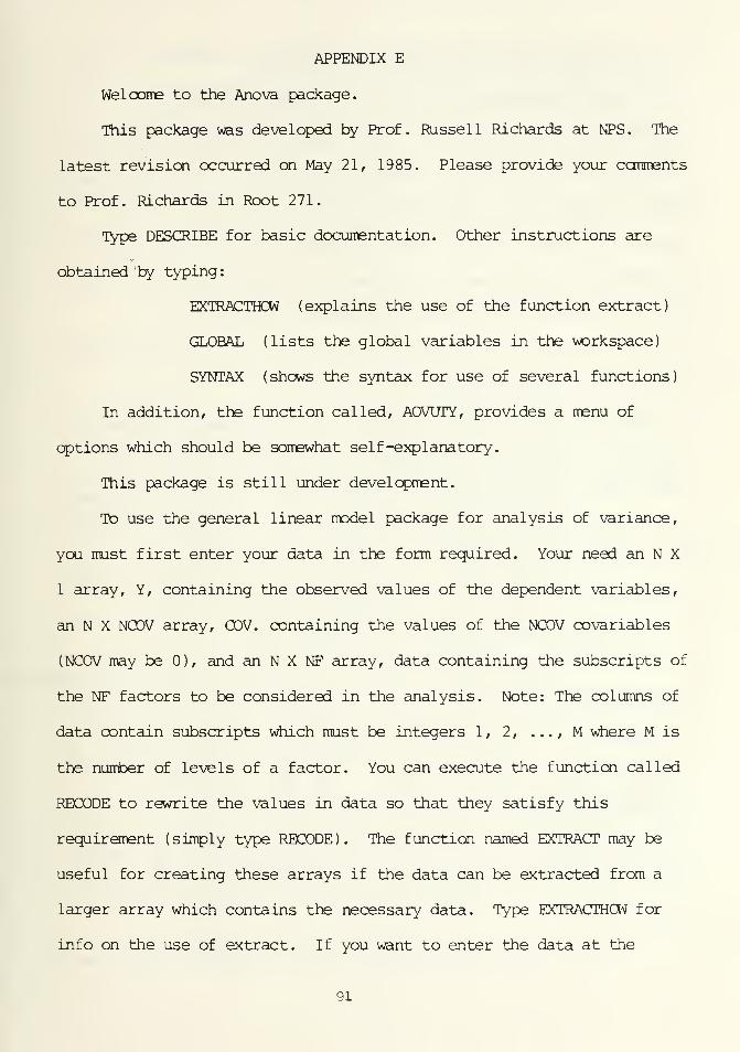
APPENDIX E

Welcome to the Anova package.

This package was developed by Prof. Russell Richards at NPS. The

latest revision occurred on May 21, 1985. Please provide your comments

to Prof. Richards in Root 271.

Type DESCRIBE for basic documentation. Other instructions are

obtained by typing

:

EXIRACTHCW (explains the use of the function extract)

GLOBAL (lists the global variables in the workspace)

SYNTAX (shows the syntax for use of several functions)

In addition, the function called, AOVUTY, provides a menu of

options which should be somewhat self-explanatory.

This package is still under development.

To use the general linear model package for analysis of variance,

you must first enter your data in the form required. Your need an N X

1 array, Y, containing the observed values of the dependent variables,

an N X NCOV array, GOV. containing the values of the NCOV covariables

(NCOV may be 0), and an N X NF array, data containing the subscripts of

the NF factors to be considered in the analysis. Note: The columns of

data contain subscripts which must be integers 1 , 2 , . . . , M where M is

the number of levels of a factor. You can execute the function called

RECODE to rewrite the values in data so that they satisfy this

requirement (simply type RECODE). The function named EXTRACT may be

useful for creating these arrays if the data can be extracted from a

larger array which contains the necessary data. Type EXIRACTHCW for

info on the use of extract. If you want to enter the data at the

91

terminal, you can use the function called INPUT.

After the necessary data are entered into the workspace,

type RUN to begin the analysis (the argument indicates the initial

run with the given data; for subsequent runs using the same data, enter

RUN 1). For the first run with a given set of data you will be

prompted to enter various information needed by the program. This

information includes names for the factors, covariables, and for the

job. It also asks if you want to transform the data. If so, the

original values of the dependent variable are stored in the array OIDY

and a new Y array is created.

With the initialization completed, you will be asked to enter the

interactions desired to be included in the analysis (if any). You

should enter the interactions by typing a vector containing the numbers

of the factors which comprise the interactions. For example, if you

want to include interactions between factors 1 and 2; factors 1 and 3;

and factors 1, 2, and 3 you should enter the vector 12 13 123.

The program then performs the following tasks:

1. A matrix D having N rows and a number of columns which depends

the number of levels of each of the NF factors is generated. This is

the portion of the design matrix corresponding to the main effects. It

contains only the values 0, 2, and -1. The main effects are

automatically normalized so that the main effects sum to 0. A

bookkeeping array, DF, of size NF X 2 is also generated. The elements

of the ith row of BF indicate which cols of D correspond to the ith

factor

.

2. An array, DD containing N rows is generated. The number of

92

cols of DD depends on the number of interactions and the number of

levels of each interaction. DD is that portion of the overall design

matrix which corresponds to the interaction terms. Like D, DD contains

only the values 0, 1, and -1. A scalar, NI, indicating the number of

interactions is created, and a bookkeeping array, Bl of size NI X 2 is

generated. It indicates which cols of DD correspond to which

interactions

.

3. The overall design matrix X, is generated by catenating COV,

D, and DD.

4. The design matrix is checked to see if it is nonsingular. If

not nonsingular, the rank is determined and a set of cols that can be

eliminated is indicated. If the design matrix can be made nonsingular

by elimination of one or more cols from the interaction set, that is

done automatically. If not, program execution terminates.

5. The analysis of variance is performed on the model, Y = XBETA.

Output consists of the R-squared statistic, the ANOVA table with the

covariable effects. The main effects and the interaction effects all

indicated. For each effect, the degrees of freedom, the sum of

squares, the mean square, and an F ratio are presented. The error and

total sums of squares and degrees of freedom are also given. Finally,

summary statistics for each of the covariables and for the dependent

variable for each level of each of the main effects are provided. This

information consists of the observation counts. The mean, the

variance, and the standard deviation. The summary statistics are given

for the original data, not the transformed data.

6. Available at the conclusion of the run is a GLOBAL vector called

93

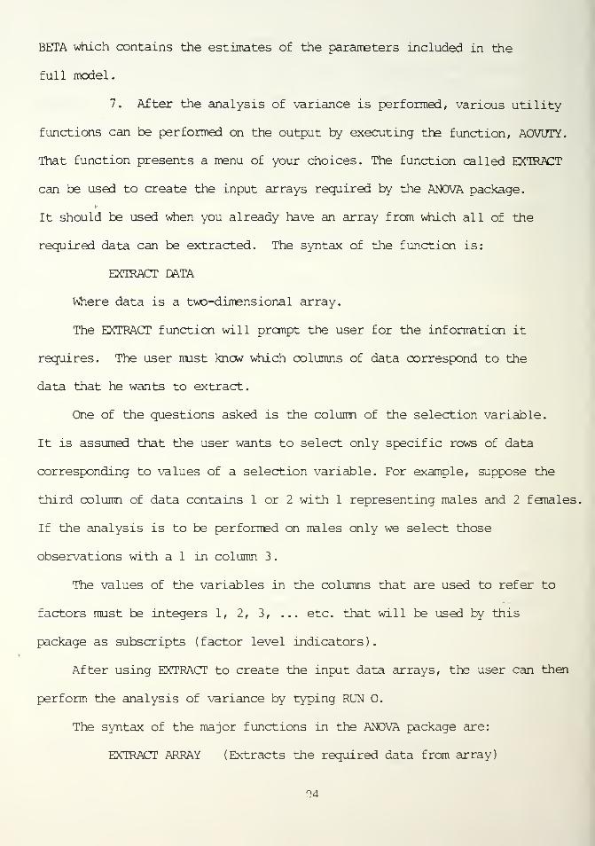
BETA which contains the estimates of the parameters included in the

full model.

7. After the analysis of variance is performed, various utility

functions can be performed on the output by executing the function, AOVUTY.

That function presents a menu of your choices. The function called EXTRACT

can be used to create the input arrays required by the ANOVA package.

It should be used when you already have an array from which all of the

required data can be extracted. The syntax of the function is:

EXTRACT DATA

Where data is a two-dimensional array.

The EXTRACT function will prompt the user for the information it

requires. The user must know which columns of data correspond to the

data that he wants to extract.

One of the questions asked is the column of the selection variable.

It is assumed that the user wants to select only specific rows of data

corresponding to values of a selection variable. For example, suppose the

third column of data contains 1 or 2 with 1 representing males and 2 females.

If the analysis is to be performed on males only we select those

observations with a 1 in column 3.

The values of the variables in the columns that are used to refer to

factors must be integers 1, 2, 3, ... etc. that will be used by this

package as subscripts (factor level indicators).

After using EXTRACT to create the input data arrays, the user can then

perform the analysis of variance by typing RUN 0.

The syntax of the major functions in the ANOVA package are:

EXTRACT ARRAY (Extracts the required data from array)

04

RECODE (Operates on the GLOBAL array data)

INPUT (Creates the arrays needed for run)

RUN K (K is 0, 1, or 2)

AOVUTY GLOBAL (Consists of various useful utility functions)

This provides a description of the GLOBAL variables used by the ANOVA

package. The convention used in naming GLOBALvariables is to always

use underscored names for GLOBAL variables.

Y - The vector of values of the dependent variable.

N - The number of observations in Y.

NCOV - The number of covariables to be considered.

COV - The array of size N by NCOV containing the values of the NF.

NF - The number of factors to be considered.

DATA - The array of size N by NF containing the subscripts of the

NF factors for each of the N observations.

D - The design matrix containing N rows of the values 0, 1, and

-1 corresponding to the main effects to be considered in the model.

The number of cols of D depends on the number of levels of the NF factors.

A factor having K levels will have K-l cols in D. K-l dunrny variables will

be defined with values or 1. The Kth level is defined so that the sum

of the effects is zero.

BG - This is an array of size NF by 2 containing bookkeeping info

concerning which factors correspond to which columns of D.

DD - This is an array of N rows containing the portion of the overall

design matrix corresponding to the interactions to be considered.

It consists entirely of the values 0, 1, and -1. The number of cols of DD

depends on the factors and interactions considered.

95

LIST OF REFERENCES

1. Soetrisno, H., Prediction of Academic Performance of theU. S. Navy Officer Students in the Operations Research/Systems Analysis Curriculum at the Naval PostgraduateSchool , M.S. Thesis, Naval Postgraduate School, MontereyCalifornia, March 1975.

2. Naval Postgraduate School Technical Report NPS 54-81-001,The Prediction of College Achievement from the ScholasticAptitude Test and the High School Record , by R. A. Weitzman,February 1981.

3. U. S. Department of the Navy, Office of the Chief of NavalOperations, Notice 1520, 9 May 1984.

4. Naval Postgraduate School Catalog, 1985.

5. Catalogue of Self -Study Courses , Naval Postgraduate SchoolMonterey, California, 1984-1985.

6. Gourman, J., The Gourman Report , pp. 160-178, NationalEducation Standards 1983.

7. Neter, J., Wasserman, W., and Kutmen, M. H., AppliedLinear Statistical Models, Richard D. Irwin, Inc., 1985.

96

BIBLIOGRAPHY

Abraham, B. and Ledolter, J., Statistical Methods for Fore -

casting, John Wiley and Sons Inc., 1983.

Bibby, J. and Toutenberg, H., Prediction and Improved Estimationin Linear Models , John Wiley and Sons Inc., 1977.

Conover, W. J., Practical Nonparametric Statistics , John Wileyand Sons Inc, 1980.

Lindman, H. R., Analysis of Variance in Complex ExperimentalDesigns , /W. H. Freeman and Company, 19 74.

Searle, S. R., Linear Models , John Wiley and Sons Inc., 1971.

Naval Postgraduate School Technical Report NPS 55SE 75061,A Comparison of Prediction of Graduate Student Performance :

Is it All Worth the Bother ?, by J. Senger and R. Elster,June 1975.

Willingham, W. W., Predicting Success in Graduate Education ,

Science, pp. 273-278, 25 January 1974.

Winer, B. J., Statistical Principles in Experimental Design ,

McGraw-Hill, 1971.

97

INITIAL DISTRIBUTION LIST

No. Copies

1. Defense Technical Information Center 2

Cameron StationAlexandria, Virginia 22304-6145

2. Library, Code 0142 2

Naval Postgraduate SchoolMonterey, California 93943-5100

3. Professor A. R. Washburn 1Code

e55Ws

Naval Postgraduate SchoolMonterey, California 93943-5100

4. Professor R. R. Read 1

Code 55ReNaval Postgraduate SchoolMonterey, California 93943-5100

5. Professor J. D. Esary 1

Code 55EyNaval Postgraduate SchoolMonterey, California 93943-5100

6. Ted Calhoun, Director of Admissions 1

Code 0145Naval Postgraduate SchoolMonterey, California 93943-5100

7. CDR Thomas E. Halwachs, USN 1

Code 30Naval Postgraduate SchoolMonterey, California 93943-5100

8. CDR N. William Blatt, USN 2

8834 Shadowlake WaySpringfield, Virginia 22153

98

IQQ. r.i -7

Thesis

35543c.l

££1*039Blatt

An analysis o#^TavalOfficer student aca-

dejad^xperformance in

:he Operations Anal-ysis curriculum in

relationship to aca-demic profile codesand other factors.