an alternative portfolio theory

An Alternative Portfolio Theory

Robert Baguenault de Viéville | Raphaël Gelrubin | Edouard Lindet | Charles Chevalier

An Alternative

Portfolio Theory


4 |

Disclaimer

This document, communicated by KeyQuant SAS (“KeyQuant”), is confidential and may not be recopied, reproduced or otherwise redistributed. It has been issued for informational purposes only and nothing in this document should be interpreted as constituting legal, regulatory, tax, financial or investment advice.

The information contained herein is addressed to and directed only at professional investors and should not be relied on by any other person. It does not constitute a report, an offer or a solicitation by anyone in the United States or in any other jurisdiction in which such a report, offer or solicitation is not authorized or to, or for the account or benefit of, any US person as defined in relevant US securities laws, or to any person to whom such report, offer or solicitation is unlawful.

The information herein may be approximate. It may contain errors and/or omissions and due to rounding, numbers presented throughout may not precisely reflect performance results. It may be based on third party sources of information which are assumed to be correct and reliable but not independently verified.

This document may also contain forward-looking statements, including, but not limited to, statements that are predictions of or indicate future events, trends, plans or objectives. Undue reliance should not be placed on such statements because, by their nature, they are subject to known and unknown risks and uncertainties.

KeyQuant does not guarantee, and accept no legal liability whatsoever arising from or connected to, the accuracy, reliability, currency or completeness of any information provided herein which may be amended at any time. KeyQuant is under no obligation to provide you with an updated version of such information.

PAST RESULTS ARE NOT NECESSARILY INDICATIVE OF FUTURE RESULTS


| 5

Tabel of Contents

Part II: Portfolio Optimization: Avoid Sharp(e) Drawdowns!

I – A Follow-Up on APT Part I . . . . . . . . . . . . . . . . . . . . . . . . . . . . . . . . . . . . . . . . . . . . . 23

II – A Predictive Proxy For The Serenity Ratio . . . . . . . . . . . . . . . . . . . . . . . . . . . . . . . . . 29

III – A Practical use of The Smart Sharpe Rato Optimization . . . . . . . . . . . . . . . . . . . . . . 36


| 21

Part II : Portfolio Optimization :

Avoid Sharp(e) Drawdowns !


| 23

Avoid Sharp(e) Drawdowns !

Introduction

In this note, we seek to optimize a portfolio allocation using the Serenity Ratio1 developed in An Alternative Portfolio Theory (APT – Part 1). As a reminder, the Serenity Ratio considers

path dependent variables to more accurately measure the drawdown risk of an investment strategy. The higher the Serenity, the better, thus an investor seeks to achieve the highest Serenity possible. However, in the context of a portfolio optimization, we find that the Serenity Ratio lacks predictability: it is a proven ex-post risk indicator to evaluate drawdowns but fails to provide information on potential future deeper drawdowns. Therefore, the Serenity Ratio cannot be used by investors to optimize their portfolio allocation. The second part of this paper focuses on finding a suitable indicator that shows the same properties as the Serenity Ratio (later called proxy) which could be used in a portfolio allocation and help limit the drawdown risk. To do so, we analyze the drivers of drawdowns and we find several explanatory variables, including autocorrelation of returns. We conclude by finding a good proxy that accounts for these variables which has a stronger predictive power than the Serenity Ratio while providing better results in minimizing drawdowns.

A Follow-Up on APT Part 1

In the last part of APT Part I, we proposed an alternative Risk-Return spectrum to the classical Markowitz (1952) Return-Volatility spectrum. We showed that our measure of Penalized Risk defined as Ulcer (average risk) multiplied by Penalty Factor (CDaR/Vol) was an excellent indicator of the hidden risks of drawdowns. In the first part of this paper, we extend our reasoning by defining optimal portfolios in both Markowitz (1952) and our alternative space. To be consistent with APT Part I, we use the same HFRI Indices2 and define our portfolios over the same period (1990-2016), and we used a standard numerical optimization process

as defined in Cheklov et al. (2005).

1 See APT Part 1 – Don’t Get Trapped in a Pitfall, January 2017 - https://www.keyquant.com/Publications.2 List and description is available in the appendices. Keep in mind that all the strategies are net of the

risk-free rate.


24 |

1- In-Sample Sharpe and Serenity Ratios Optimizations

These in-sample optimizations represent the static allocation which would have maximized the Sharpe and Serenity ratios over the 1990-2016 time period, had the future been known in 1990. Figure 1 shows that the two resulting strategies would have yielded very different results. The

classic risk parity allocation (1/vol) has been added to Figure 1 and Table 1 for comparison.

In-Sample 1/Vol Allocation In-Sample Sharpe Optimization In-Sample Serenity Optimization

100

150

200

250

300

350

20152010200520001995

0%

-6%

-12%

-18%

20152010200520001995

Figure 1 NAVs of the In-Sample Sharpe and Serenity Optimization Processes

Underwater Curves of the In-Sample Sharpe and Serenity Optimization Processes


| 25

0% 10% 20% 30% 40% 50% 60% 70% 80% 90% 100%

9.4% 19.9%

49.2% 8.1% 22% 18.6%

39.6% 28.1%

■ Systematic Diversified

■ Fixed Income-Convertible Arbitrage

■ Global Macro

■ Equity Market Neutral

■ Multi-Strategy

■ Relative Value

■ Quantitative Directional

■ Event-Driven

■ S&P 500

■ Fund of Funds

■ Equity Hedge

■ Barclays US Bond Index

Sharpe Allocation

Serenity Allocation

Figure 2 Optimal In-Sample allocations

The optimal static allocations are shown on figure 2.

As the in-sample Serenity optimization represents the very best static investment an investor could have made, we will use it thereafter as our benchmark. Our goal will be to find a practical allocation methodology that yields results as close as possible to this ideal optimum.


26 |

A glossary with the definition of every risk metric used in the paper is available in the appendices. The results of each optimization are as follows:

• The Sharpe optimization offers a low volatility strategy yet cannot avoid the 2008 financial crisis losses due to its investment into convergent strategies (Equity Market Neutral and Relative value) which suffer heavy drawdowns during that period.

• The Serenity optimization offers a higher volatility yet much lower drawdowns thanks to its high investment in divergent strategies (mainly Systematic Diversified).

Serenity Optimization sharply decreases the maximum drawdown

In-Sample 1/Vol In-Sample Sharpe In-Sample Serenity Allocation Optimization Optimization

Return 4.43% 4.10% 4.89%

Volatility 4.02% 2.64% 4.16%

Sharpe Ratio 1.10 1.56 1.18

Ulcer Index 3.39% 1.68% 1.65%

UPI 1.30 2.44 2.97

Max DD 17.25% 9.11% 4.84%

CDaR 12.67% 6.29% 4.00%

Pitfall 3.15 2.38 0.96

Penalized Risk 10.7% 4.0% 1.6%

Serenity 0.41 1.03 3.08

Table 1 Statistics of the In-Sample Sharpe and Serenity Optimization Processes


| 27

2- Out-of-Sample Sharpe and Serenity Ratios Optimizations

In order to test our indicator in the context of an actual portfolio optimization on a month by month basis, we now perform an out-of-sample optimization. Out-of-Sample optimization represents the rolling allocation which would have optimized the Sharpe and Serenity Ratios over the 1990-2016 period, rebalanced on a monthly basis. Figure 3 shows the result of the optimized portfolios.

Figure 3 NAVs of the Out-of-Sample Sharpe and Serenity Optimization Processes

100

150

200

250

Out-of-Sample Serenity Optimization Out-of-Sample Sharpe Optimization

20152010200520001995

201520102005200019950%

-6%

-4%

-2%

-8%

-10%

-12%

-14%

Underwater Curves of the Out-of-Sample Sharpe and Serenity Optimization Processes


28 |

Static Sharpe Rolling Sharpe Static Serenity Rolling Serenity Optimization Optimization Optimization Optimization

Return 3.70% 3.50%

Volatility 2.88% 3.84%

Sharpe Ratio 1.56 1.28 1.18 0.91

Ulcer Index 2.56% 2.46%

UPI 2.44 1.45 2.97 1.42

Max DD 12.21% 8.00%

CDaR 9.63% 6.52%

Pitfall 3.35 1.70

Penalized Risk 8.6% 4.2%

Serenity 1.03 0.43 3.08 0.84

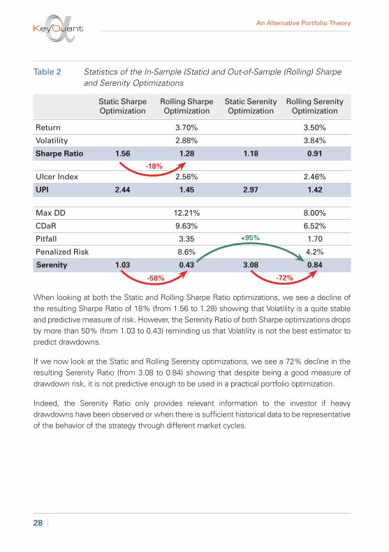
When looking at both the Static and Rolling Sharpe Ratio optimizations, we see a decline of the resulting Sharpe Ratio of 18% (from 1.56 to 1.28) showing that Volatility is a quite stable and predictive measure of risk. However, the Serenity Ratio of both Sharpe optimizations drops by more than 50% (from 1.03 to 0.43) reminding us that Volatility is not the best estimator to predict drawdowns.

If we now look at the Static and Rolling Serenity optimizations, we see a 72% decline in the resulting Serenity Ratio (from 3.08 to 0.84) showing that despite being a good measure of drawdown risk, it is not predictive enough to be used in a practical portfolio optimization.

Indeed, the Serenity Ratio only provides relevant information to the investor if heavy drawdowns have been observed or when there is sufficient historical data to be representative of the behavior of the strategy through different market cycles.

-18%

-58% -72%

+95%

Table 2 Statistics of the In-Sample (Static) and Out-of-Sample (Rolling) Sharpe and Serenity Optimizations


| 29

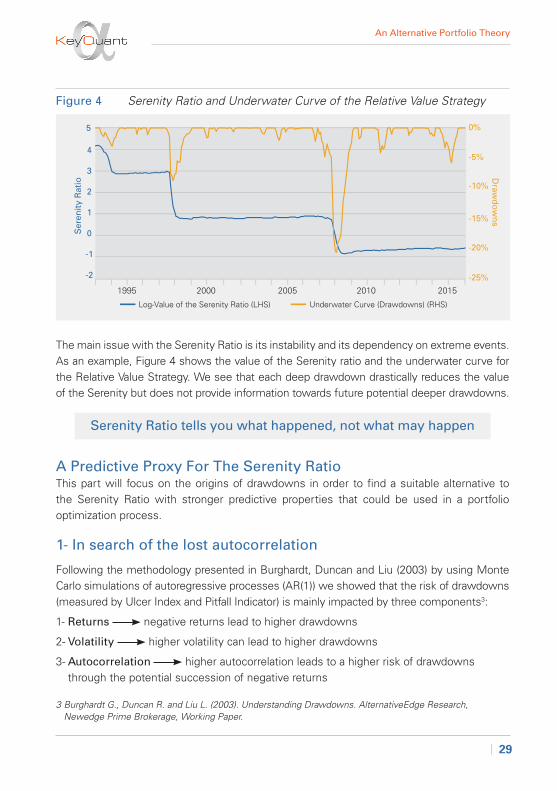
The main issue with the Serenity Ratio is its instability and its dependency on extreme events. As an example, Figure 4 shows the value of the Serenity ratio and the underwater curve for the Relative Value Strategy. We see that each deep drawdown drastically reduces the value of the Serenity but does not provide information towards future potential deeper drawdowns.

Serenity Ratio tells you what happened, not what may happen

A Predictive Proxy For The Serenity RatioThis part will focus on the origins of drawdowns in order to find a suitable alternative to the Serenity Ratio with stronger predictive properties that could be used in a portfolio optimization process.

1- In search of the lost autocorrelation

Following the methodology presented in Burghardt, Duncan and Liu (2003) by using Monte Carlo simulations of autoregressive processes (AR(1)) we showed that the risk of drawdowns (measured by Ulcer Index and Pitfall Indicator) is mainly impacted by three components3:

1- Returns negative returns lead to higher drawdowns

2- Volatility higher volatility can lead to higher drawdowns

3- Autocorrelation higher autocorrelation leads to a higher risk of drawdowns through the potential succession of negative returns

3 Burghardt G., Duncan R. and Liu L. (2003). Understanding Drawdowns. AlternativeEdge Research, Newedge Prime Brokerage, Working Paper.

20152010200520001995

0%

-5%

-10%

-15%

-20%

-25%

5

Ser

enity

Rat

io

Draw

do

wn

s

4

3

2

1

0

-1

-2

Log-Value of the Serenity Ratio (LHS) Underwater Curve (Drawdowns) (RHS)

Figure 4 Serenity Ratio and Underwater Curve of the Relative Value Strategy


30 |

0

Autocorrelation

0.2-0.2 0.4-0.4 0.6-0.6 0.8-0.8 1-1

9

8

7

6

5

4

3

2

1

0

Ris

k o

f DD

= U

lcer

Risk o

f Extrem

e DD

= Pitfall

45%

40%

35%

30%

25%

20%

15%

10%

5%

0%

Ulcer Index CDaR

While return and volatility are accounted for in the classic Sharpe approach, autocorrelation is ignored.

Figure 5 shows the impact of autocorrelation on the risk of drawdowns.4 The exponential shape of both the Ulcer Index and the Pitfall Indicator curves show that higher levels of positive autocorrelations tend to produce very dangerous drawdowns that would result in an investment blow-up sooner or later.

Table 5 Impact of the Autocorrelation on the risk of Drawdowns

4 Based on simulations of AR(1) processes with a Mean of 5%, volatility of 10% and controlling for autocorrelation.

The same analysis of the impact of return and volatility is available in the appendices.

As a conclusion, a risk measure which takes into account returns, volatility and autocorrelation

could be a good predictor of drawdowns and act as a proxy of the Serenity Ratio.


| 31

2- The Smart Sharpe Ratio

In The Statistics of Sharpe Ratio (Lo (2002)), it is shown that the actual time aggregation of the Volatility using the square root of time is a simplification of the real formula for annualizing the Volatility. The formula that is widely used by the industry to annualize the Volatility of an asset by multiplying the daily/monthly volatility by either or disregards the potential autocorrelation. The more accurate formula is5:

Where is the annualized variance of a portfolio based on the variance calculated on periods and the different autocorrelation coefficients at lag .

Should a process have all its autocorrelation coefficients equal to zero the formula becomes:

We find the widely-used formula for the annualization of volatility, which gives

A parallel can be made between the Serenity formula and the accurate Sharpe formula:

Where both Volatility and Ulcer represent an average risk and and

represent a penalty factor affecting the average risk.

For the remainder of this paper, the standard Sharpe Ratio will be referred to as Traditional Sharpe Ratio while the accurate Sharpe Ratio taking autocorrelations into account will be referred as Smart Sharpe Ratio. The similarities between the Serenity Ratio and the Smart Sharpe make the latter a potential candidate as a proxy for future optimization. The next part will focus on verifying that the instability of Serenity Ratio (due to the instability of the Extreme Risk Penalty) is corrected in the Smart Sharpe.

The Smart Sharpe Ratio could act as a Proxy for the Serenity Ratio by penalizing autocorrelation

5 Demonstration in the appendices.


32 |

3- Stability of the Smart Sharpe Ratio

The main purpose of the Serenity Ratio was to penalize strategies with a hidden risk of drawdowns which could not be reflected in the sole value of the volatility. This feature has been transposed to the Smart Sharpe Ratio through the use of autocorrelation as shown previously (Fig. 5). We now need to verify the stability (hence the potential predictability) of the measure to make the Smart Sharpe Ratio a good proxy.

The stability issue in the Serenity Ratio relies mainly on the instability of the Extreme Risk Penalty. For example, the following graph shows the value of the Extreme Risk Penalty (CDaR/Vol) and the Autocorrelation Penalty (

) for the Relative Value and the

Systematic Diversified Strategies6:

2015201020052000

0

20

40

60

80

100

120

Relative Value Autocorrelation Penalty

Syst. Div. Autocorrelation Penalty

Relative Value Extreme Risk Penalty

Syst. Div. Extreme Risk Penalty

+22%

+92%

We see that the 2008 financial crisis has a very significant impact on the value of the Extreme Risk Penalty of the Relative Value (92% growth from 56.9 to 109), showing once again the dependency of Serenity (through CDaR) to extreme events. In the meantime, the Autocorrelation Penalty only moves by 22% (from 90 to 110) showing that our new Penalty Factor is a more stable value. This is also true when looking at the stability of the Autocorrelation Penalty of the Systematic Diversified strategy. The same analysis on other strategies is available in the appendices.

Figure 6 Autocorrelation Penalty and Extreme Risk Penalty

6 We chose to rebase both Penalty Factors of the Relative Value Strategy to 100 at the end of 2016 for comparison.


| 33

Therefore, the Smart Sharpe Ratio shares the main properties of the Serenity Ratio regarding drawdowns and its Penalty Factor is more stable than the Serenity Ratio which makes it a very suitable proxy to test in an optimization process to confirm its superior predictive power. The Serenity Ratio will however remain our risk measure of choice to compare ex-post strategies.

Smart Sharpe Ratio is a good proxy of the Serenity Ratio


34 |

201520102005200019950%

-6%

-4%

-2%

-8%

-10%

-12%

-14%

75

150

100

200

250

Out-of-Sample TraditionalSharpe Optimization

Out-of-Sample Serenity Optimization

Out-of-Sample SmartSharpe Optimization

20152010200520001995

Figure 7 NAVs of the Traditional Sharpe, the Serenity and the Smart Sharpe Optimization

Underwater Curves of the Traditional Sharpe, the Serenity and the Smart Sharpe Optimization

4- Smart Sharpe Ratio Out-of-Sample Optimization

The result of out-of-sample optimization confirms that the Smart Sharpe Ratio can be

used in a portfolio allocation to improve the drawdown profile of an investment and

therefore its Serenity Ratio. The following graphs present the NAVs and the underwater

curves of the Traditional Sharpe, the Serenity and the Smart Sharpe strategies:


| 35

Traditional Sharpe Serenity Ratio Smart Sharpe Ratio Optimization Optimization Optimization

Return 3.70% 3.50% 3.72%

Volatility 2.88% 3.84% 3.06%

Traditional. Sharpe 1.28 0.91 1.22

Smart Sharpe 0.97 0.91 1.12

Ulcer Index 2.56% 2.46% 1.68%

UPI 1.45 1.42 2.21

Max DD 12.2% 8.0% 7.0%

CDaR 9.63% 6.52% 5.61%

Pitfall 3.35 1.70 1.84

Pen Risk 8.6% 4.2% 3.1%

Serenity 0.43 0.84 1.21

Table 3 shows the improvements we progressively made starting from a Traditional Sharpe optimization to a Smart Sharpe Optimization. Starting from a Serenity Ratio of 0.43, using the autocorrelation as a proxy for the risk of drawdowns, we were able to increase the Serenity up to 1.21. Moreover, the Sharpe Ratio of the Smart Sharpe Optimization shows that using autocorrelations in an allocation process does not trade off the risk of volatility for a risk of drawdowns but tends to minimize both.

Table 3 Statistics of the Out-of-Sample Traditional Sharpe, Serenity and Smart Sharpe Optimization Processes

x 2

≈

x 1.5

The Smart Sharpe Optimization confirms its ability to anticipate drawdowns with the

use of auto-correlations compared to the Traditional Sharpe Optimization. The strategy

also offers the best Serenity Ratio of all optimizations by having fewer drawdowns

(lower Ulcer) and a very good CDaR as shown in the following statistics.


36 |

The Smart Sharpe is good at managing the average risk of drawdowns (Ulcer Index of the out-of-sample Smart Sharpe Optimization is 1.68%, very close to its in-sample-value of 1.65%, cf. Table 1). However, it is less efficient in reducing unexpected drawdowns as they are not as well measured through autocorrelations which can represent a possible improvement of the measure.

The superior predictive power of the Smart Sharpe Ratio offers much better drawdown control while preserving the Sharpe Ratio

A Practical use of the Smart Sharpe Ratio Optimization

1- Results of a constrained out-of-sample optimization

The previous optimization did not consider problems and constraints many allocators may face. In order to be closer to these requirements, we fixed the following constraints when calculating the optimal portfolio7:

• All metrics are calculated with a 98% exponential smoothing average

• Allocation in each asset is capped at 20% maximum

• Weights can only move by 4% each month

We decided not to constrain any investment in any particular asset class (such as Equity or Bonds) even though many investors may face these requirements. The main purpose of this optimisation is to understand how these asset classes can compose a better portfolio using the Smart Sharpe Ratio.

The results of the optimizations over the 1999-2016 period8 are presented on Figure 8 and Table 4 (see below).

7 Robustness checks on the parameters have been performed to ensure the consistency of the results.

8 Here we dropped the 1990-1999 period because it does not represent a differentiation period for the strategies.


| 37

20152010200520000%

-4%

-8%

-12%

-16%

-20%

75

1/Vol Allocation Traditional Sharpe Optimization Smart Sharpe Optimization

75

150

100

200

1/Vol Allocation Traditional Sharpe Optimization Smart Sharpe Optimization

2015201020052000

Figure 8 NAVs of the Traditional Sharpe and Smart Sharpe Optimization Processes

Underwater Curves of the Traditional Sharpe and Smart Sharpe Optimization Processes


38 |

1/Vol Traditional Sharpe Smart Sharpe Optimization Optimization

Return 3.34% 3.47% 3.53%

Vol 3.87% 2.88% 3.15%

Traditional Sharpe 0.86 1.20 1.12

Smart Sharpe 0.67 1.11 1.14

Ulcer 4.02% 2.05% 1.43%

UPI 0.83 1.69 2.47

Max DD 17.88% 8.94% 5.90%

CDaR 15.53 % 7.62% 4.63%

Pitfall Indicator 4.01 2.64 1.47

Penalized Risk 16.1% 5.4% 2.1%

Serenity 0.21 0.64 1.68

Figure 8 and Table 4 show the importance of taking autocorrelations into account when optimizing a portfolio. The drawdown control offered by the Smart Sharpe Portfolio is better than the Traditional Sharpe Portfolio while keeping similar Sharpe Ratios. The average risk of drawdown is vastly reduced with an Ulcer Performance Index (UPI) of 2.47 for the Smart Sharpe Optimization versus a UPI of 1.69 for the Traditional Sharpe Portfolio. The global risk of the strategy is also reduced as illustrated in the value of the Serenity Ratio of the Smart Sharpe strategy which is more than two times the value of the Serenity of the Traditional Sharpe strategy (1.68 vs. 0.64).

Table 4 Statistics of the Out-of-Sample Traditional Sharpe, Serenity and Smart Sharpe Optimization

x 2.6


| 39

25%

20%

15%

10%

5%

0%

■ Allocation towards Systematic Diversified in our Approximate Sharpe Allocation

■ Real Allocation towards Managed Futures amongst the Hedge Fund Industry

■ Real Allocation towards Systematic CTA amongst the Hedge Fund Industry

2015201020052000

Figure 9 Allocation in Systematic Diversified (CTA), Barclays Hedge

Are Investors Truly Using Sharpe Ratio?!

We have compared the allocation to Systematic Strategies actually made by investors with our previous Traditional Sharpe allocation.

The divestment in Systematic Diversified Strategies after major financial turmoil, as seen between 1999 and 2008, and since 2013 is reflected in the actual allocation investors made towards CTAs.


40 |

0%

20%

40%

60%

80%

Allo

catio

n

100%

LTCM +RussianCrisis

Dot-ComBubbleBurst

GlobalFinancial

Crisis


■ Global Macro



■ Fund of Funds

■ Multi-Strategy



■ Event-Driven

■ Relative Value

■ S&P 500

■ Equity Hedge

2015201020052000

Figure 10 Optimal Allocation with the Traditional Sharpe

Figure 10 shows the weighting evolution of the portfolio allocation based on the Traditional Sharpe Ratio using the constraints defined previously. Using the Traditional Sharpe Ratio an investor won’t have a very stable allocation through time. Following the Russian and LTCM crisis that occurred at the end of 1998, the fear of a more global propagation to the economy leads to a portfolio with a maxed-out allocation towards crisis alpha strategies (20% in Systematic Diversified). As the Russian crisis fades away and the dot-com bubble slowly deflates the investment in crisis alpha strategies is progressively reduced. The reduction of Systematic Diversified to the benefit of strategies with lower volatility but a higher risk of drawdowns is typical of the Traditional Sharpe Ratio optimization. The portfolio looks for higher returns and lower volatility even though the risk of potential future crisis still exists. The position in Systematic Diversified is only progressively rebuilt as the 2008 crisis unfolds and reaches a maximum just before the market turning point, therefore not providing enough crisis alpha during the heat of the market downturn. By doing this, investors can improve their short-term performance but these small gains risk being wiped out when the next downturn occurs. By being always one beat late regarding their investments, investors who reduce their exposure to CTAs trade small gains in an already positive environment for more risk of losing much more when things go sour.

2- Portfolio Allocations


| 41

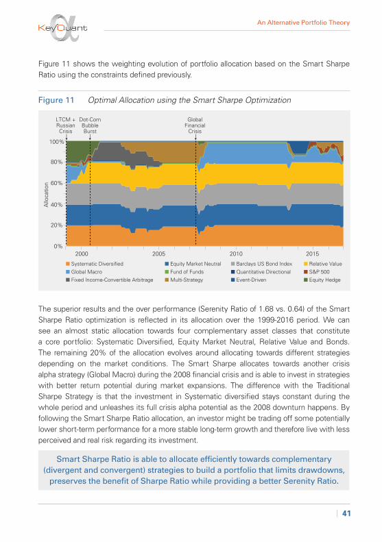
Figure 11 shows the weighting evolution of portfolio allocation based on the Smart Sharpe Ratio using the constraints defined previously.

The superior results and the over performance (Serenity Ratio of 1.68 vs. 0.64) of the Smart Sharpe Ratio optimization is reflected in its allocation over the 1999-2016 period. We can see an almost static allocation towards four complementary asset classes that constitute a core portfolio: Systematic Diversified, Equity Market Neutral, Relative Value and Bonds. The remaining 20% of the allocation evolves around allocating towards different strategies depending on the market conditions. The Smart Sharpe allocates towards another crisis alpha strategy (Global Macro) during the 2008 financial crisis and is able to invest in strategies with better return potential during market expansions. The difference with the Traditional Sharpe Strategy is that the investment in Systematic diversified stays constant during the whole period and unleashes its full crisis alpha potential as the 2008 downturn happens. By following the Smart Sharpe Ratio allocation, an investor might be trading off some potentially lower short-term performance for a more stable long-term growth and therefore live with less perceived and real risk regarding its investment.

Smart Sharpe Ratio is able to allocate efficiently towards complementary (divergent and convergent) strategies to build a portfolio that limits drawdowns,

preserves the benefit of Sharpe Ratio while providing a better Serenity Ratio.

0%

20%

40%

60%

80%

Allo

catio

n

100%

LTCM +RussianCrisis

Dot-ComBubbleBurst

GlobalFinancial

Crisis


■ Global Macro




■ Event-Driven

■ Relative Value

■ S&P 500

■ Equity Hedge

2015201020052000


■ Fund of Funds

■ Multi-Strategy

Figure 11 Optimal Allocation using the Smart Sharpe Optimization


42 |

Conclusion

Following the Alternative Portfolio – Part 1, the purpose of this paper was to allocate a portfolio in order to maximize the Serenity Ratio. Because of its latency issues, Serenity Ratio cannot be used to optimize a portfolio, but only as an ex-post measure. Through the use of autocorrelations, we were able to find a proxy - The Smart Sharpe Ratio - that shares the properties of the Serenity Ratio and has better predictive properties. The resulting portfolio shows a greater stability in its allocation, limits the drawdown risk and provides a better Serenity Ratio while preserving the Sharpe Ratio. Therefore, investors who want to minimize their drawdown, should aim to maximize their Serenity Ratio by using the Smart Sharpe optimization.


| 43

References and

Appendices


44 |

References – Part II

[1] Allen D., McAleer, M, Powell, R., and Singh A. (2015). Down-side Risk Metrics as Portfolio Diversification Strategies across the GFC. Tinbergen Institute Discussion Paper.

[2] Burghardt G., Duncan R. and Liu L. (2003). Uderstanding Drawdowns. AlternativeEdge Research, Newedge Prime Brokerage, Working Paper

[3] Burghardt G. and Liu L. (2012). It’s the Autocorrelation Stupid. AlternativeEdge Research, Newedge Prime Brokerage, Working Paper

[4] Chekhlov A., Uryasev S. and Zabarankin M. (2003). Portfolio Optimisation with Drawdown Constraints, Working Paper.

[5] Chekhlov A., Uryasev S. and Zabarankin M. (2005). Drawdown measure in portfolio optimization. International Journal of Theoretical and Applied Finance, 8(1), 13 58.

[6] Getmansky M., Lo A. and Makarov I. (2004). An economic model of serial correlation and illiquidity in hedge fund returns. Journal of Financial Economics 74 (2004) 529-609.

[7] Goldberg L. and Mahmoud O. (2015). Drawdown: From Practice to Theory and Back Again, Working Paper.

[8] Harris R., Mazibas M. (2013). Dynamic hedge fund portfolio construction: A semi-parametric approach. Journal of Banking & Finance 37 (2013) 139–149.

[9] KeyQuant (2017). An Alternative Portfolio Theory, Don’t Get Trapped in a Pitfall!. KeyQuant White Paper Series

[9] Lo A. (2002). The Statistics of Sharpe Ratio. Financial Analyst Journal, July/August 2002 36-52.

[10] Markowitz H. M. (1952). Portfolio selection. Journal of Finance 7(1) 77–91.

[11] Rosenberg M., Tomeo J. F., and Chung. S. Y. (2004). Hedge Fund-of-Funds Asset Allocation Using a Convergent and Divergent Strategy Approach. State Street Global Advisors. Working Paper.

[12] Rzepczynski. (1999). Market Vision and Investment Styles: Convergent versus Divergent Trading. The Journal of Alternative Investment, Winter 1999 77-82.


| 45

Appendices – Part II

1- Glossary

Metric Definition Extra Info Ulcer Index Root Mean Square Measure of the average Risk of Drawdowns of Drawdowns (the lower the better)

UPI (Ulcer Return “Sharpe Ratio”-like Indicator Performance Index) UPI = Ulcer Index (Return over Average Risk of Drawdowns) (the higher the better)

CDaR(95%) Average of the 5% Measure of the Extreme Risk of Drawdowns “biggest” drawdowns (the lower the better)

Pitfall Ind. CDaR(95%) Penalty Factor - Measure of the Extreme Vol Risk of Drawdowns in number of volatilities (the lower the better)

Penalized Risk Ulcer x Pitfall Measure of the Global Risk of Drawdowns (lower is better)

Serenity Return “Sharpe Ratio”-like Indicator Pen. Risk (Return over Global Risk of Drawdowns) (the higher the better)


46 |

2- HFRI Indices

HFRI Names Short Name Strategies Included

HFRI Macro: Systematic Systematic Diversified Managed Futures, Diversified Index Trend Following (HFRIMTI Index)

HFRI EH: Equity Market Equity Market Neutral Quantitaztive Equity Market Neutral Index Neutral Strategies (HFRIEMNI Index)

HFRI EH: Quantitative Directional Quantitative Directional Factor-Based and Statistical (HFRIENHI Index) Arbitrage Trading Strategies

HFRI FOF: Diversified Index Fund of Funds Investment in a variety of strategies (HFRIFOFD Index) among multiple managers

HFRI RV: Fixed Income-Convertible Fixed Income- Relative Value Strategies limited Arbitrage Index (HFRICAI Index) Convertible Arbitrage to Fixed Income and Convertible Instruments

HFRI RV: Multi-Strategy Index Multi-Strategy Relative Value Strategies on (HFRIFI Index) Fixed Income, derivatives, Equity, Real Estate and/or MLP Assets

HFRI Event-Driven (Total) Index Event-Driven Event Driven Strategies (HFRIEDI Index)

HFRI Equity Hedge (Total) Index Equity Hedge Long-Short Equity Strategies (HFRIEHI Index)

HFRI Macro (Total) Index Global Macro Global Macro Strategies (HFRIMI Index)

HFRI Relative Value (Total) Index Relative Value Relative Value Strategies (HFRIRVA Index)

S&P 500 (SPXT Index) S&P 500 S&P 500

Barclays US Bond Index Barclays US Bond Index US Bonds (LBUSTRUU Index)


| 47

3- Smart Sharpe Ratio Demonstration

In this annex, we show that:

Considering the case of IID returns, we note the returns over periods:

We have:

This can be represented as the sum of the coefficients of the following matrix of size :

The matrix being symmetric, we split the sum in two parts, the sum of the diagonal coefficients and two times the sum of the upper triangle:

For the second part of the Sum we see that by adding through the consecutive diagonals we have:

Then:


48 |

4- AR(1) Filter

Due to the monthly granularity of our data set and the fact that the Smart Sharpe Ratio needs high lags of autocorrelations to be calculated, we have decided to apply an AR(1) filter on autocorrelations to limit the impact of estimation errors.

An AR(1) process is defined as follows:

Where is a white noise.

We can show that and .

Using this formula, we see that the calculation of the Smart Sharpe Ratio is made easier by only estimating the first autocorrelation coefficient and deriving the following coefficient from the first. This method prevents side effects in the calculation such as “negative” volatilities, non-exponentially decreases in the correlograms, etc.

An example with the global Macro strategies showing estimation errors on high lags autocorrelation causing side effects on the calculation of the Smart Sharpe Ratio is shown below:

-20%

-10%

0%

10%

20%

30%

40%

50%

60%

1 2 3 4 5 6 7 8 9 10 11 12

Global Macro Strategies Correlogram

Global Macro Global Macro with AR(1) Filter Significance Level


| 49

5- Impact of Return and Volatility on the Risk of Drawdowns

A strategy with negative returns would more likely suffer bigger drawdowns than a strategy with positive returns. This is confirmed by the simulations of an AR(1) process where the autocorrelation has been set to 0 and volatility to 10% controlling for returns between -10% and 10%, the risk of drawdowns (DD) diminishes as returns gets higher.

Higher volatility leads to higher average and extreme drawdowns as both Ulcer and Pitfall increase with volatility. The convergence of the Pitfall Indicator is due to the fact that when volatility is high compared to the returns, drawdowns of more than 95% occur therefore capping the value of CDaR to a maximum.

Mean Return

0 5% 10% 15%-5%-10%-15%

10

8.75

7.5

6.25

5

3.75

2.5

1.25

0

Ris

k o

f D

D =

Ulc

erR

isk of E

xtreme D

D = P

itfall

80%

70%

60%

50%

40%

30%

20%

10%

0%

Ulcer (LHS) Pitfall (RHS)

Volatility

0 5% 10% 15% 20% 25%

4

3.2

2.4

1.6

0.8

0

Ris

k o

f D

D =

Ulc

erR

isk of E

xtreme D

D = P

itfall

30%

25%

20%

15%

10%

5%

0%

Ulcer (LHS) Pitfall (RHS)


50 |

6- Penalty Factors

The following graphs represent the stability of the Autocorrelation Penalty compared to the Extreme Risk Penalty for other Strategies than those presented in Figure 6.

2015201020052000

Fund of Funds Autocorrelation Penalty Fund of Funds Autocorrelation Penalty

0

10

20

30

40

50

60

70

80

90

100

2015201020052000

Global Macro Autocorrelation Penalty Global Macro Extreme Risk Penalty

0

10

20

30

40

50

60

70

80

90

100


| 51

2015201020052000

Event-Driven Autocorrelation Penalty Event-Driven Extreme Risk Penalty

0

20

40

60

80

100

120

2015201020052000

Equity Hedge Autocorrelation Penalty Equity Hedge Extreme Risk Penalty

0

20

40

60

80

100

120


52 |

Notes

Authors

Robert Baguenault de Viéville, Founding Partner & Fund ManagerGraduate of ESTACA and with a Master’s degree from HEC, Robert Baguenault de Viéville began his career as a quantitative researcher with a subsidiary of Man Investments specializing in managing futures. In 2007, he co-founded his first research company focused on systematic trading with Raphaël Gelrubin. In 2009, he co-founded the investment management company KeyQuant.

Raphaël Gelrubin, Founding Partner & Fund ManagerGraduate of the University Paris - Dauphine and ENSAE, Raphaël Gelrubin began his career as a quantitative researcher focused on risk within a subsidiary of Man Investments specializing in managing futures. In 2007, he co-founded his first research company focused on systematic trading with Robert Baguenault de Viéville. In 2009, he co-founded the investment management company KeyQuant.

Edouard Lindet, Research AnalystEdouard joined the investment research team of KeyQuant in January 2016. He previously interned as a quantitative analyst with KPMG in Paris and Alken Asset Management in London. He holds a graduate degree from École Nationale de la Statistique et de l’Administration Économique (“ENSAE”) with a specialization in Market Analysis and Corporate Finance.

Charles Chevalier, Research AnalystCharles joined the investment research team of KeyQuant in October 2016 as a PhD candidate. He previously interned as a quantitative analyst with Amundi and BNP Paribas Investment Partners in Paris. He holds a graduate degree from École Nationale de la Statistique et de l’Analyse de l’Information (“ENSAI”) with a specialization in Financial Engineering and a MSc in Finance from Université Paris Dauphine.

20 rue Quentin-Bauchart

75008 – Paris – France

T. +33 1 84 13 83 00

[email protected]

www.keyquant.com

an alternative portfolio theory

Documents