an adaptive finite element method for linear elliptic problemsfrey/ftp/m5105/eriksson k., an... ·...
TRANSCRIPT
MATHEMATICS OF COMPUTATIONVOLUME 50, NUMBER 182APRIL 1988, PAGES 361-383
An Adaptive Finite Element Method for
Linear Elliptic Problems
By Kenneth Eriksson and Claes Johnson
Abstract. We propose an adaptive finite element method for linear elliptic problems
based on an optimal maximum norm error estimate. The algorithm produces a sequence
of successively refined meshes with a final mesh on which a given error tolerance is
satisfied. In each step the refinement to be made is determined by locally estimating
the size of certain derivatives of the exact solution through computed finite element
solutions. We analyze and justify the algorithm in a model case.
Introduction. Recently, adaptive finite element methods for elliptic problems
have attracted much interest, see, e.g., [l]-[4], [6], [7], [13], and are rapidly be-
coming increasingly important in applications. The basic problem concerning such
adaptive methods is roughly the following: Given an elliptic problem with no a pri-
ori knowledge of the behavior of the exact solution and a finite element method for
this problem together with an error tolerance 8 > 0 and a certain norm, construct
an automatic procedure for finding a finite element mesh such that the error in the
corresponding finite element solution is at most 6 in the given norm. One further
requires the constructed mesh to be efficient in the sense that, e.g., the number
of elements is nearly minimal. A typical adaptive procedure could be expected to
involve a sequence of finite element solutions on successively refined meshes (start-
ing with, e.g., a quasi-uniform mesh), and the procedure would end when the error
is smaller than or equal to the given tolerance. At each step of the procedure an
estimate of the error on the given mesh would be made, and in case the error toler-
ance is not met, a refined mesh to be used in the next step would be constructed.
Typically, the procedure would generate meshes which are refined in regions where
the exact solution is nonsmooth such as, e.g., neighborhoods of corners in a polyg-
onal domain. In the methods proposed by BabuSka and coworkers [2]-[4], the error
estimate at each step is based on solving local problems involving a local residual,
and the refinements are carried out according to the size of the solutions of the
local problems. This method seems to produce reasonable meshes in many cases
but appears to be difficult to theoretically justify in several dimensions (cf. [2], [4]).
The purpose of this note is to present and analyze, in a model case, an adaptive
procedure which is based on a different approach than the BabuSka method. As a
model problem we shall consider the Poisson equation
{ -Au = f in 0,(0.1) I
' { u = 0 onT,
Received June 24, 1985; revised October 16, 1986.
1980 Mathematics Subject Classification (1985 Revision). Primary 65N15, 65N30.
©1988 American Mathematical Society0025-5718/88 $1.00 + $.25 per page
361
License or copyright restrictions may apply to redistribution; see http://www.ams.org/journal-terms-of-use
362 KENNETH ERIKSSON AND CLAES JOHNSON
in a bounded domain fi in the plane with boundary T. We shall consider the
standard finite element method for (0.1) using continuous piecewise linear functions
on a triangulation Tn = {K} of fi into triangles K of diameter hx- We shall assume
that we want to control the gradient of the error in the maximum norm (cf. Remark
1.2 below). The error control will be based on an optimal a priori estimate of the
form (cf. [17], [8])
(0.2) ||V(u - u/l)||oo,n < C0 max hK\u\2t00tK,K€Th
where for m = 0,1,..., and w a domain,
Mm.oo.u, = SUp \Dav(x)\, Nloo.u, = Mo.oo.w,XÇ.UJ
\a\=m
and where uh denotes the finite element solution. Here we use the usual multi-index
notation Dav for dérivâtes of order |q|. Further, Co denotes a positive constant
assumed for the moment to be known approximately (the problem of roughly esti-
mating Co is commented on in Remark 3.1 below). Given now a tolerance 6 > 0,
we want to find a finite element solution uh satisfying ||V(u — u'l)||0o,n < S, and
thus (0.2) leads us to the following choice of the local mesh size hx-
(0.3) C0hK\u\2tOO<K ~6.
The obvious idea is now to seek to estimate the quantity |t¿|2,oo,K by using computed
finite element solutions uh and then determine the local mesh size according to (0.3).
We shall present below an algorithm for error control and adaptive mesh selection
based on this approach. We shall then consider a model situation where the exact
solution has a singularity in fi of a certain form, and we shall in this very special
case verify that the proposed algorithm will generate a sequence of meshes leading
to a final correctly refined mesh on which the error tolerance is met. The basic
technical tool to prove this result is a localized version of the a priori estimate (0.2).
Using this estimate we prove that it is possible to locally estimate with sufficient
accuracy the desired quantity |u|2,oo,k by using certain (local) difference quotients
of computed gradients of uh. Thus, we may say that our adaptive algorithm is
based on an optimal a posteriori error estimate of the form (0.2) with |u|2,oo,k
replaced by an approximation obtained through the computed solution uh. We are
presently developing this approach also for adaptive mesh control in time and space
for parabolic problems ([10], [11], [14], [15]) and hyperbolic problems ([12]).
The analysis of this note, in which we consider for simplicity the case of an
interior singularity on a smooth domain, can be extended to cover problem (0.1)
with fi a convex polygonal domain (and / smooth), in which case the exact solution
has singularities of strength r13, ß > 1, at the corners, see Eriksson [9], where also
further extensions to nonconvex polygonal domains corresponding to ß > \ are
given.
The general idea of basing an adaptive method on estimating the derivatives of
the exact solution through computed approximate solutions of course is not new
and has been used extensively in an intuitive, qualitative only and nonautomatic
way in engineering computations. An early paper proposing to base an adaptive
method on an energy norm error estimate and to estimate the derivatives of the
License or copyright restrictions may apply to redistribution; see http://www.ams.org/journal-terms-of-use
AN ADAPTIVE FINITE ELEMENT METHOD 363
exact solution involved through computations, is given by [7]. A similar approach
was also taken in [6] and [16]. Our method is based on the same idea but we extend
the setting by considering different norms (cf. Remark 1.2 below), by seeking to
justify the algorithm theoretically and also by considering the problem of estimating
e.g. the constant Co in (0.2) to make the error control fully quantitative, cf. Remark
3.1 below.
Extensions of the presented results to more general elliptic problems, for instance
variable coefficient linear problems, or to higher-order finite elements, seem to be
possible. As soon as we have a sharp error estimate together with a local maximum
norm error estimate at hand, there is a possibility of using this as a basis for an
adaptive procedure. In particular, this means that error estimates which have been
considered to be of mostly theoretical interest, in fact may be of key importance in
the practical implementation of the finite element method on real life problems in
the future!
An outline of this note is as follows. In Section 1 we present the adaptive
algorithm. In Sections 2 and 3 we analyze this algorithm in a model case and prove
that in this case it performs as desired. Finally, in Section 4 we present the results
of some numerical experiments with a particular implementation of the algorithm
which show that indeed the algorithm performs in practice as expected.
We shall assume that all finite element meshes Tn that occur satisfy a minimum
angle condition, i.e., we assume that there is a positive constant 0 such that all
angles of all K 6 Th for all Th are greater than or equal to 0. Below, we will by c
and C denote various positive constants which will be independent of the meshes
Th and thus of the corresponding finite element solutions uh. The constants may
depend on the minimal angle 0, the domain fi and on the exact solution u (more
precisely on the constants c and C in (2.1)).
1. The Adaptive Algorithm. We shall consider the following standard finite
element method for the Poisson equation (0.1): Given the finite element mesh
Th = {K}, find uh e Vh such that
(1.1) a{uh,v) = (/,«) VueVfc,
where Vh is the space of piecewise linear continuous functions v on the triangulation
Th vanishing on T, and
a(v,w) = I Vv -Vwdx, (v,w) = / vwdx.Jn Jn
We assume that we start with a quasi-uniform mesh T^ = {K} with elements K
satisfying c6 < ch < hx < Ch. To take h > cö is reasonable since otherwise the
initial mesh would be unnecessarily fine in areas where the solution is smooth.
To compute approximations of the derivatives Dau with |a| = 2 locally, we
shall apply certain difference operators D]j to the computed gradient Vuh. The
difference operators DH will be of the form
D]1V(X) = V{X±1HH)-V{X\
with 7 = (1,0) or 7 = (0,1). Here, H = Chx if x e K, and C is a sufficiently
large constant, the choice of which will be made precise below. If x is close to the
License or copyright restrictions may apply to redistribution; see http://www.ams.org/journal-terms-of-use
364 KENNETH ERIKSSON AND CLAES JOHNSON
boundary, the point x ± ^¡H is chosen so as to belong to fi. We will thus use first-
order difference operators DH involving translations of size H which will typically
be of the order of a couple of local mesh widths.
The algorithm can now be formulated as follows:
Io. Choose Th = Tjj- where T^ is the initial quasi-uniform mesh.
2°. Given a mesh Th, compute the corresponding finite element solution uh 6
vh.3°. Compute the following quantity for each x 6 K e T/¡:
(1.2) D2Huh(x) = uisx{\DlDauh(y)\ : |a| = |7| = 1, \y - x\ < Ch},
where h = miiiKeTh hx and C is a sufficiently large constant.
4°. If for all K e Th we have
(1.3) C0hKDH(uh;K)<ë,
where
D2H(uh;K) = max D2Huh(x),
then stop and accept the finite element solution uh. If not, construct a new
mesh Th by minimally refining the old mesh Th so that for each K 6 Th
(1.4) CohkD2H{uh; K)<8 VA e fh with K C K.
Then redefine Th = fh and return to 2°.
Remark 1.1. Note that to compute D2H(uh;K), only local simple computations
are involved; cf. Section 4 below for the particular implementation of the algorithm
used in the numerical experiments. The quantity D2H{uh;K) is basically to be
thought of as an approximation of |w|2,oo,ä"- For technical reasons, D2H(uh;K)
involves difference quotients at points in an ^-neighborhood of K. Variants of this
procedure are possible. For instance, we may take C = 0 in (1.2) and avoid the
maximization if we require the meshes Th to have a certain "stiffness", guaranteeing
that the mesh size does not change too quickly (see [9]). D
Remark 1.2. One may choose to control the error in norms other than the |-|i)0o,n
norm used in (0.2). For example, we may take as starting point a maximum norm
estimate of the form (cf., e.g., [8], [17], [18], [19])
(1.5) ||u - uh||oo,n < C0 max h2K\u\2f00tK,n ii . KeTh
where the constant Co here also includes a logarithmic dependence of min/i/f, or
the standard energy norm estimate
(1-6) |u - ti*|ll3,n < Co ( J2 hK\u\h,K\xeTh
where | ■ |m,2,w denotes the seminorm of highest-order derivatives in the Sobolev
space Hm(oj). In case (1.5), we would use the above algorithm with hfc in (1.3) and
(1.4) replaced by h2K. The estimate (0.2) would be used also in this case to prove
that Dfi(uh;K) is a sufficiently good approximation to |u|2,c»,/ci cf. the analysis
•■i*
License or copyright restrictions may apply to redistribution; see http://www.ams.org/journal-terms-of-use
AN ADAPTIVE FINITE ELEMENT METHOD 365
below. In case (1.6), the new mesh Th in 4° would be constructed so that
h2kD2H(uh;K) ~ 7 = constant, VÄ" G fh with K Ç K,
Co T.1 } =C0VNt = 6,
where TV is the number of elements in Th- Again, (0.2) would be used to justify
the algorithm. Note that (1.5) and (1.7) give the same control up to the choice of
the tolerance 8. For numerical experiments with error control based on (1.5), see
Section 4 below. For a further discussion, see [9]. □
Remark 1.3. In any adaptive method we face two problems, namely, (i) esti-
mation of the error and check if the error is below the given tolerance, and (ii)
construction of a properly refined new grid if the error is above the tolerance. It is
not enough to solve just problem (i). Even if we can accurately estimate the error
e(x) for all x € fi, it is not clear how to properly refine the mesh to decrease the
error, if too large. In general, one should not refine everywhere where the error is
too large since in an elliptic problem some effects are global, for instance, a corner
singularity may cause a large error also away from the corner. To decrease the error
in such a case, we should not refine everywhere but only close to the corner. A
main difference between the Babuska approach and our approach is that we base
the adaptive algorithm on an error estimate which exhibits the structure of the
error and which is used to solve both problems (i) and (ii). It appears to us that
in the Babuska approach it is less obvious how to solve (ii), and that this is the
reason why this method is more difficult to justify theoretically. D
2. Analysis in a Model Case.
2.1. The Exact Solution. We shall now analyze and justify the proposed adaptive
algorithm under the assumption that the exact solution u belongs to the Sobolev
space W^(ii) and satisfies the following estimate: There are constants c and C
such that for all x €E fi,
(2.1a) c\x\0-2 < D2u(x) < C\xf-2,
(2.1b) |ZFit(x)| < C|x|^"3 for H = 3,
where
D2u{x) = max{|L>aii(z)| : \a\ = 2},
and 1 < ß < 2. Note that this corresponds to a situation where the exact solution
u(x) has a singularity at the origin of strength \x\0. For simplicity we assume
that the origin belongs to the interior of fi. A more realistic situation would be to
consider the case of a singularity located at a corner of fi; a singularity of strength
\x\P with 1 < ß < 2 would then correspond to a corner angle k = ir/ß satisfying
7r/2 < k, < it. Of course the restriction ß > 1 is related to the fact that we seek to
control the quantity ||Vu||oo,fi! which requires UVul^n to be bounded, whereas
we assume ß < 2 to have a singularity of sufficient strength for a refinement to be
necessary.
Observe that in applying the algorithm in the above case we do not, of course,
use any a priori knowledge of the nature of the exact solution like (2.1). The only
License or copyright restrictions may apply to redistribution; see http://www.ams.org/journal-terms-of-use
366 KENNETH ERIKSSON AND CLAES JOHNSON
data required for the algorithm is fi, / and 8. What we prove is that if (2.1) is
satisfied, then the algorithm will perform as desired.
To simplify the presentation, we shall further assume that the region fi is con-
vex with smooth boundary T. The functions v in the finite element space Vh are
assumed to be piecewise linear on the triangulation Th = {K}, corresponding to a
polygonal approximation fi/¡ of fi, and extended by zero in fi \ Í2V
2.2. Optimal Meshes. Let us now first see what a reasonable mesh would look
like in the case (2.1), assuming that we want to satisfy (0.3). It is then convenient
to divide fi into subregions ÍX, according to the size of the second derivatives of u.
We thus introduce
Üj = {xGÜ: 2~3 <|x|<2-J+1},
and we assume that IJi>o ^i = ^- We tnen nave by (2-1)
(2.2) cdßr2 < lula,«,^ < Cd0'2,
where dj = 2_J. From (0.3) it follows that we should choose the mesh size h3 in
fij so that hjd. ~ 8, i.e.,
(2.3) hj ~ 8d2~0
as long as hj < dj, i.e., as long as j < J, where
(2.4) d*fl~6.
Here and below, we write a ~ b if ca < b < Ca. Further, we should choose the
mesh size ~ ¿VC-i) in fi} = {x € fi: \x\ < 2~J}. It is clear that the choice (2.3)
is best possible, and we shall prove below that our algorithm will produce a final
mesh satisfying (2.3).
2.3 Analysis of Step 1. We first recall the following optimal global maximum
norm estimate (cf. [17]): For the finite element method (1.1) on the quasi-uniform
mesh Tj; with solution uh we have for 0 < s < 1
(2.5) ||V(« - t/)||oo,n < CÄ8|«|s+i,eo,o,
where | • |s,oo,o denotes the norm in the usual Sobolev space W¿,(fi) of functions
with derivatives of order s in Loo(fi). Let us now start the analysis of the algorithm
in the special case of an exact solution u € W^(Q) satisfying (2.1). We then begin
with the quasi-uniform partition T^ with elements of size h and the corresponding
finite element solution uh. We shall use the following local version of the estimate
(2.5) with 8 = 1, which states that the finite element error in Qj is comparable to
the interpolation error in Qj, if dj/h is large enough.
LEMMA 2.1. There are constants C and C\ such that, if dj > C\h, then
(2.6) l|V(tt-u*)||00fni<CWf-a.
Below we shall give an extension of Lemma 2.1 to more general meshes. This
result, which is the key technical result we will need, involves a generalization of
the earlier estimate (2.5) to non-quasi-uniform meshes and also, as indicated, a
localization.
We postpone the proof of Lemma 2.1 and first show how this result can be used
to prove that D2Huh(x) will be a reasonable approximation of D2u(x) for x G il, if
H/h and dj/h are big enough. More precisely, we shall prove the following result.
License or copyright restrictions may apply to redistribution; see http://www.ams.org/journal-terms-of-use
AN ADAPTIVE FINITE ELEMENT METHOD 367
LEMMA 2.2. There are constants c, C and C such that, if H — Ch, then
(2.7b) ch0~2 < |£>^u*(a;)| < Ch0"2 if \x\ < Ch.
Proof. We have by (2.1) and Lemma 2.1, if x G fi¿, dj > 2Cjl, dj > 2H,
\a\ = |7| = 1,
\D1HDauli(x) - Di+au(x)\ < |DjL>Q(u* - u)(x)\ + \{D]j- D^)Dau{x)\
<^d0-* + CHd0-\
where we used a standard approximation result to estimate the second term. Now,
if we here choose H = Ch and dj > CH with C sufficiently large, then it follows
that
(2.8) ID^D^ix) - Di+au{x)\ < \D2u(x)
if x G fij, dj > Ch and H — Ch. Further, by the global estimate (2.5) with
s = ß — 1 and an inverse estimate it also follows that there is a constant C such
that, if H > h, then
(2.9) |Z?£Dau*(z)| < Ch0'2.
Recalling now the definition (1.2), we easily obtain the desired estimates (2.7a,b)
by combining (2.1), (2.8) and (2.9) (note that the constant C in (1.2) is assumed
to be the same as the constant C in the lemma). G
By Lemma 2.2 we may use uh to accurately compute a local mesh size hj in
fij satisfying (2.3), if dj > Ch, i.e., knowing uh, we may decide on a reasonable
refinement in {|x| > Ch) (for simplicity we write {\x\ < d} to mean {x G fi: |x| <
d}). In the region {|i| < Ch} we will, by (2.7b), be led to a refinement with_2-/3
mesh size c8h . Thus, if in stage 4° of the algorithm the stopping criterion is
not satisfied, a new mesh Th will be constructed which is a refinement of the first
quasi-uniform mesh T-^ and which will have the following characteristics (here h(x)
is a measure of the mesh size at x):
(2.10a) h{x) ~ 8d2~0 if x G fi.,, dj > Ch,
(2.10b) h{x) ~ h := 8h2~0 if \x\ < Ch,
where 8 < Ch ; in fact, we have assumed that h > c8 and h < C. This means
in particular that the mesh T/, obtained after the first quasi-uniform mesh T-^ will
be correctly refined in {|z| > Ch} and will be quasi-uniform in {\x\ < Ch} with
typical mesh size h~8h
2.4 Analysis of Step 2. We now continue the analysis starting with a mesh Th
with local mesh size h(x) satisfying (2.10). We shall in this case use the following
generalizations of Lemmas 2.1 and 2.2, the difference being that the mesh is now
no longer quasi-uniform.
License or copyright restrictions may apply to redistribution; see http://www.ams.org/journal-terms-of-use
368 KENNETH ERIKSSON AND CLAES JOHNSON
LEMMA 2.3. Suppose the meshTh satisfies (2.10). Then there are constants C
and Ci such that, if dj > C\h, then
(2.11) IIVtu-ti^Hocn, <Ch2d0'2,
where, according to (2.10), h3 := max((5<i ~ ,8h ) is the local mesh size on fij.
LEMMA 2.4. Suppose that the mesh Th satisfies (2.10). Then there are con-
stants c, C and C such that, if x G K n fi,, dj > Ch and H = Chx, then
c<\D%u^)\<- \D2u(x)\
further, if\x\ < Ch and H = Ch, then
ch0-2<\D2Huh{x)\<Ch0-2.
The proof of Lemma 2.3 will be given below. The proof of Lemma 2.4 is analogous
to the proof of Lemma 2.2 above and relies on Lemma 2.3.
From Lemma 2.4 it follows that D2Huh{x) will be a reasonable approximation of
D2u(x) in {|a;| > Ch}. Thus, if the stopping criterion is not satisfied, the algorithm
will produce a refinement T), of Th with the following characteristics:
(2.12a) h(x) ~ 8d2~0 if x G Qj, ci, > Ch,
(2.12b) h(x) ~ h ■= 6h2-0 if \x\ < Ch,
and 8 < Ch0"1. Redefining now Th = Th and letting h and h take the roles of
h and h, we then have again the same situation as at the start of Step 2 at the
beginning of this subsection, i.e., a mesh Th satisfying (2.10). The process may now
be repeated.
2.5. The Number of Steps: Statement of Main Result. Let us now see how many
steps will be required to obtain a mesh on which the error tolerance is satisfied.
For simplicity, we start with a quasi-uniform mesh T^ with mesh length h = 8. We
denote by hn the minimal mesh length of the triangulation Th = TJ¡ obtained after
n steps. According to (2.10b), we will then have
hn = 8hl-_1, n>l,
where JXq = h = 8, and consequently
k=c?=ô8^ht~r= ¿¿(2-/3) . . . ¿(2-/3)" =¿(l_(2-/3)"+1)/(/3-l)!
so that
(2.13) /jg-^ii-O-«"-".
Now, as a by-product of the proof of Lemma 2.3, we have the following error
estimate which gives a generalization of (2.5) to a non-quasi-uniform mesh: If Th
satisfies (2.10) then
||V(u-ti*)||oo,n <Chß-\
In particular, we thus have, recalling (2.13),
(2.14) ||V(« - «iJHocn < Cht1 = C8^2-0^1.
License or copyright restrictions may apply to redistribution; see http://www.ams.org/journal-terms-of-use
AN ADAPTIVE FINITE ELEMENT METHOD 369
This means that we will not in a finite number of steps achieve ||V(w - uh)||oo,o <
C8. In practice, this does not of course pose a problem; we may, e.g., assume that
n is chosen so that¿-(2-/3)" + ' < C
with C a moderate constant. The qualitative conclusion from (2.14) is that the
required number of steps would (slowly) increase as ß approaches 1, ß > 1.
We can now summarize our main result as follows:
THEOREM. Suppose the exact solution u satisfies (2.1). Then the adaptive al-
gorithm with initial mesh length h = 8 will produce a sequence of meshes T£,
n = 0,1,2,..., with corresponding finite element solutions u£ (uq — uh), such that
WViu-u^lUnKCS^2-0^1.
Further, the mesh T£ will be correctly refined in the region {\x\ > Chn_x} where
hn_1, the minimal size of elements in T£~l, is given by
&»-!=«'". 0n = (1- (2 -ß)n)/(ß -1),
and the region {\x\ < Chn_1} will have a quasi-uniform mesh of size hn.
3. Proofs of Lemmas 2.1 and 2.3. It remains to prove the local estimate
(2.11) of Lemma 2.3. Clearly Lemma 2.1 can be viewed as a special case of Lemma
2.3 and does not require a separate proof. For the proof of Lemma 2.3 we fix j
and an arbitrary point xo G fiJ; together with the element Ko containing xo, for
which we may assume dist(¿Yo, 0) ~ dj. We let ùh G Vj, denote the piecewise linear
interpolant of u and write <9j := d/dxi, i — 1,2.
For the interpolant uh we have
||V(U - ÜÄ)||oo,Jf0 < ChKo\U\2,oo,K0 < Ch3d0-2,
and hence, by the triangle inequality,
\dt(u - uh)(xo)\ < Ch3d0-2 + \di(ük - uh)(x0)\.
Since di(ûh — uh) is constant on Ko, the last term can be represented as
\d%(üh -uh){xo)\ = \(dl(üh -uh),8o)\,
where ¿o is a smooth approximate delta function, supported in Äoi and such that
^Jfoll^olloo.ifo < C.
Thus,
\dt(u - uh)(x0)\ < Ch3d0-2 + \(di(üh - uh),80)\
<C/iJdy"2 + l(öi(w-«/,),^)|,
where we have again used the triangle inequality. Let now G solve the adjoint
problem- AG = d%80 in fi,
G = 0 on T,
and let Gh G Vh be the Ritz projection of G determined by
a{v,G-Gh) = 0 Vv€Vh.
License or copyright restrictions may apply to redistribution; see http://www.ams.org/journal-terms-of-use
370 KENNETH ERIKSSON AND CLAES JOHNSON
Then,
(dl(u - uh), 80) = -(« - uh,dt8o) = -(u - uh, -AG)
(3.1) = -a(u -uh,G) = a(u -uh,Gh - G) = a(u - üh, Gh -G).
Below we shall show, with e := Gh - G, that
(3-2) ||Ve||Ll(n)<C,
and
(3-3) ||Ve||n;+2< Cd"1,
where || • ||u denotes the L2(w)-norm and fi£ = {x G fi: |x| < 2~k} as above. Using
(3.1), (3.2) and (3.3), together with approximation properties of the interpolant ùh,
we find
\(di(u-uh),8o)\ = \a{u-üh,e)\
< ¿2 \W«-üh)\Unk\\Ve\\Ll(rik)+C E l|V(«-^)||oo,n,4||Ve||nfck<j+2 k>j+2
< maxo||V(«-«'l)||0O,nlt||Ve||Ll(n)
+ c\ E liv(n-ùh)||^nt4] ||ve||n.+2\k>j+2 J
<C max hkd0-2 + C[ E h2kd2k0-2\ dj1
- \k>j+2 J
< Ch3d0-2,
where in the last step we have used the definitions of dk and hk to get
max hirdî' = max max(8h d.~ ,8)k<j+2 " k<]+2 v fc '
= max(é/i2 ßdß-2,8) = hj+2d0~2 < Chjd0-2
and
E hfâ0-2= E <52max(^4-2V-2,^)k>j+2 k>j+2
<282max(h1-20 E 40-2, E dl\ k>j+2 k>3+2
< C82msx(h4-20d20-2,d2) = Ch2d20-2.
In order to prove Lemma 2.3, it now suffices to verify (3.2) and (3.3). For this
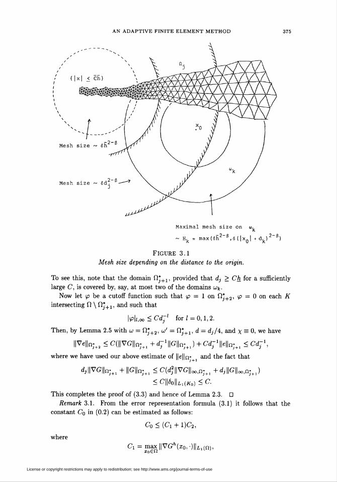
purpose we introduce the domains (cf. Figure 3.1)
Wfc = {z G fi: 2~k < \x - x0| < 2"fc+1}
and
w¡ = {i£íl: |x-x0| <2~k}.
License or copyright restrictions may apply to redistribution; see http://www.ams.org/journal-terms-of-use
AN ADAPTIVE FINITE ELEMENT METHOD 371
For the proof of (3.2) we have first
||Ve||Mn) = E HVelk("*) + IIVe|klK) < CS + Cdj\\Ve\\u.,k>J
where
5:=E4||Ve|U,k<j
and where J will be determined later. For the moment we only assume that J is
not too big so that whenever k < J and K intersects wk, K G T/¡, then K Ç u'k :=
u>k-i U (¿k U ijJk+i- We shall prove below that for a suitable choice of such a J, we
have
(3.4) S<C + Cdj\\Ve\\u.+±S,
and
(3.5) dj||Ve||u;<C.
Together, these estimates will complete the proof of (3.2). For the proofs of (3.4)
and (3.3), we shall need the following local error estimate.
LEMMA 2.5. There is a constant C such that the following holds: Ifw Ç u' C f!,
d := dist(w,fi \ uj') > 0, and diam(Ä') < |d whenever K intersects u, K G Th,
then
||Ve||w < C inf (||V(G - X)IU +d~1\\G - xV) + CdT1]^,.x£Vh
Proof. Let \ G Vh be arbitrary and put c = Gh — x and n = x - G, and let ip
be a smooth cutoff function such that <p = 1 on w, <p = 0 on each K intersecting
fi \ w', and
(3.6) Mi,oo<Cd-' for / = 0,1,2.
Using integration by parts and the error equation
a(v,e) = (Vu,Ve) = 0 Vv G Vh,
we find that, with || • || — || • ||n,
ll*>V?||3 = (Vb2?), Vf) - 2(çV<p, <pVç)
, 7) = (V(^2Ç), Ve) - (V( A), Vr,) - 2(çVç>, pVç)
= (V(*>2? - (<p2?)h), Ve) - (V(^2ç), Vr,) - 2(çV<p, pVç)
= (V(^2ç - (p2ç)h), Vf) - (V(pa ?)*, Vr?) - 2(ÇV^, pV?),
where (p2ç)'1 G Vj, denotes the piecewise linear interpolant of <p2ç satisfying
(3.8) ||V^2ç)*||<C||V(A)l|,
(3.9) ||V(^2c: - (<p2ç)h)\\K < ChK E \\Da(<P2c)\\K VKGTh.
I«l = 2
We shall now estimate the three terms on the right-hand side of (3.7). By (3.9)
and (3.6), together with the fact that ç is piecewise linear, and using an inverse
License or copyright restrictions may apply to redistribution; see http://www.ams.org/journal-terms-of-use
372 KENNETH ERIKSSON AND CLAES JOHNSON
estimate on each K, we obtain
\(V(<p2ç-(p2c)h),Vç)\
<c E Md-^MiK + d-ipVfiiiOiiViii*K
KCu'
<c E^'iifii^ + ii^fii^^'iifiiifK
KCu'
<Cd-2||c||2, + i|bVc||2.
Using (3.8), we find that
|(V(^a$')h,Vf7)|<C7||V(¥)ai)lll|ViïL.
<Gd-%||», + i||pVf||a + C||Vii|ß,.
Finally,
|2(çV^^VÇ)|<Cd-2|k||2, + i||^Vf||2.
Altogether we now have
||^VÇ||2<C(d-2||Ç|!2, + ||Vr/||2,) + |||^Vç||2,
and hence
||^Vc||<C(d-1||r||w- + ||Vr?|U).
For the error e, this implies
||Ve||w < IbVfH + HVrjIU < Cid-'WçW^ + ||Vîj||w.)
<C{dT1\\ri\\u> + d-1\\4u> + \\Vri\\U'),
which completes the proof of Lemma 2.5. G
We now continue with the proof of Lemma 2.3 with the purpose of first showing
(3.4) and (3.5), and then (3.3). Applying Lemma 2.5 with ui — wk and u/ = oj'k,
X = Gh the piecewise linear interpolant of G, and
Hk:=8max(h , (|x0| +dk)2"0) ~ max hKKCu'k
(cf. Fig 3.1), we obtain
5=E^I|Ve|U<C E (*l|V(G-Gfc)|U + ||G-G*||Wà + |WU)k<J k<J+l
<c E (dkHk + H2)\G\2,2,Uk+c E IHU-k<J+2 k<J+l
In order to estimate |G|2,2,w*) we use the representation
DaG(x)= [ D%g(x,y)dt8o(y)dy
= - / diD^g(x, y)8Q(y) dy, x <£ K0,JKo
where g(x, y) is the associated Green's function, known to satisfy
(3.10) \DlD2g(x,y)\<C\x-y\-3-™ for \a\ = 2,|7| = 0,1.
License or copyright restrictions may apply to redistribution; see http://www.ams.org/journal-terms-of-use
AN ADAPTIVE FINITE ELEMENT METHOD 373
Hence,
and so
|G|2,2,Wt < Cdk max max \DaG(x)\ < Cdk2\\80\\Ll{Ko) < Cd,-|a|=2 zfc^jt
E (dkHk + H2)\G\2,2,Uk<C E {d-klHk + d-k2H>k<J+2 k<J+2
Kcil + maxd^H^^d^H,,
^ ' k<J
where in the last step we have used the facts that dk l < 4dfc^2 and Hk < Hk-2.
Below we shall choose J in such a way that
d~,lHj ^maxdr1^ < C.J k<J h ~
J2dk'1Hk = ^28max(h2~0dk-1,(\xo\+dk)2-0dk1]
k<J
Further,
,-2-omax
k<J k<J
<C¿max U^E^1' l^ol^E^1' E4"T2-^V^^-l U_|2-/3\-^^-l Y^i-/?
k<J k<J k<J
<C8mäx(h2~0d-j\ \xo\2-ßdj1,dj-0)
<C8rmx(h2~0d-j\(\xo\+dj)2-0d-jl)
^CHjd-j1.
Hence we conclude that
s<c+ E IML-k<J+l
Let us now estimate ||e||Wfc. We have that
\\e\\Mk = sup(p,e),
where the supremum is taken over all <p with support in u>k and with ||^||Wt = 1.
For such a ip, let (p be the solution of the adjoint problem
—Atp = ip in fi,
4> = 0 on r,
and let <f>h G Vh be the piecewise linear interpolant of </>, so that
\(<p,e)\ = \a(d>,e)\ = \a(<p-]>h,e)\
< E HV(* - ¿")IU IIVeL, + ||V(0 - ^)\\u. ||Ve||w.i<j
< C E «|2,2,u.¡ II VeL, + CHj\<t>\2>2^jA || Ve||w..i<j
Here,
|0|2,2,w, < Cd¡min(d,""2,d^2)dfe.
License or copyright restrictions may apply to redistribution; see http://www.ams.org/journal-terms-of-use
374 KENNETH ERIKSSON AND CLAES JOHNSON
For I < k — 2 and I > k + 2, this follows from the representation
Da<p{x) = JD°g(x,y)<p(y)ds,
using (3.10), and for k — 1 < / < k + 1, it is a consequence of the standard elliptic
regularity estimate
Wa.a.o < C|M|.
Estimating |0|2,2,w*_ by similar arguments, we find that
||e|U < C^H^imnid]-2,dk2)dk\\Ve\\u¡ + CHJdjdk1\\Ve\\u)-J,i<j
and by changing order of summation we conclude
E l|e|k<CEllVeL«^d' E <4nun(dr2,d-:k<J+l 1<J k<J+l
+ CHjdj\\Ve\l: E dkk<J+l
<CE#H|Ve|L + Ctfj ||Ve||w}i<j
< C» maxiHidJ-^S + CHj\\Ve\\u-.
In order to complete the proof of (3.4) we now choose J such that
¿<^1=^drl-¿-
It remains to show that (3.5) holds for this choice of J. We then note that by
stability we have ||Ve|| < ||VG||, where
||VG||2 = a(G,G) = (G,dl80) = -(dlG,80) < ||VG|| \\80\\k0.
Together, these estimates show that
dj||Ve|| < dj||VG|| < dj\\6o\\Ko < CdjhK\ < C,
where, in the last step, we have used that
dj ~ C.Hj < C8 max(h2~0, \xo\2~0, d2f0),
implying, since 8 < Ch , that
dj<C8max(h , |x0|2_/3) ~ /ijf0-
It now remains to prove (3.3). For this we first note that as a part of the proof
of (3.4) we have shown that
E IHU<c,k<J+l
which in turn implies that
Nn;+1 < C
License or copyright restrictions may apply to redistribution; see http://www.ams.org/journal-terms-of-use
AN ADAPTIVE FINITE ELEMENT METHOD 375
Maximal mesh size on u
~ Hk = max(Sh2 ß , 6 ( | xQ | + dk) 2 &)
Figure 3.1
Mesh size depending on the distance to the origin.
To see this, note that the domain fi*+1, provided that dj > Ch for a sufficiently
large C, is covered by, say, at most two of the domains wk.
Now let <p be a cutoff function such that <p = 1 on fi*+2, <P = 0 on each K
intersecting fi \ fi*+1, and such that
Mi,oo<Gd-' for/= 0,1,2.
Then, by Lemma 2.5 with w = fij+2> w' = fi}+1, d = dj/4, and x = 0, we have
||Ve||n;+2 < G(||VG||n;+l +<Ç-1||G||n;+1) + Gd-1||e||n;+1 < Cdj\
where we have used our above estimate of Hello- and the fact that
^l|VG||n;+1 + ||C||o;+1 < C(d2\\VG\UQ-+l +dJ||G||00,n;+1)
<C\\8o\\LliKa)<C.
This completes the proof of (3.3) and hence of Lemma 2.3. D
Remark 3.1. From the error representation formula (3.1) it follows that the
constant Co in (0.2) can be estimated as follows:
Co < (Cj + 1)C2,
where
G1 = max||VGfc(x0!-)IU1(O),zo€W
License or copyright restrictions may apply to redistribution; see http://www.ams.org/journal-terms-of-use
376 KENNETH ERIKSSON AND CLAES JOHNSON
with Gh(x0, •) the discrete Green's function with pole at xo G fi occurring in (3.1),
and where C2 is the error constant in interpolation with piecewise linear functions:
\u - ùft|i,oo,n < C2 max hK\u\2ooK.K€Th
The constant C2 depends on the minimal angle of the triangulation T/, and may
easily be estimated (on reasonable triangulations one can probably take C2 ~ 2
in practice). Note that C\ essentially depends only on fi (and the coefficients in
a variable coefficient generalization of (0.1)) and not on the right-hand side /. To
compute C\ approximately, it may in many cases be sufficient to compute Gh(xo, ■)
on a coarse mesh for only a few conveniently chosen points xo G fi (see [9]).
4. Numerical Results. In this section we give the results of some numerical
experiments with the following variant of the algorithm analyzed above, where 3°
and 4° are replaced by:
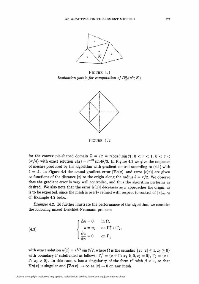
3°'. For each K G Th find Vuh(PK) at the center of gravity PK of K and also
Vuh(Pk') for the set N(K) of neighboring triangles K' G Th with one side
in common with K (see Figure 4.1) and set
WM. m iW)-^(p„)i|a| = l \PjK - "K']K'eN(K)
4°'. If for all K G Th
(4.1) hKD2H(uh;K)<8,
then stop and accept the finite element solution uh. Otherwise, construct
a new mesh Th by repeatedly subdividing each triangle into four equal
triangles until
(4.2) hkD2H{uh;K)<8 VA" G fh with K Ç K.
This algorithm essentially corresponds to the algorithm of Section 1 with Co = 1,
C = 0 and H = hK.
To implement the algorithm, we used the PLTMG-code by R. E. Bank [5] and
simply replaced the Babuska type adaptivity, originally present in this code, by
our own adaptivity. We kept the following feature of the original PLTMG-code:
Successive meshes Th are chosen so that the number of degrees of freedom increases
by approximately a factor of 4. This means that in 4°' the repeated subdivisions
are only carried out as long as this condition is met. As a result, a somewhat larger
number of steps than theoretically necessary is sometimes taken in practice. Notice
also that in the PLTMG-code 'transition elements' obtained by subdivision into
two triangles (obtained by introducing the dotted lines in Figure 4.2) are used to
connect triangles with different subdivisions.
Such dotted lines are removed before and reintroduced after continued subdivi-
sions, which means that no triangles with small angles will be constructed during the
refinement process unless such triangles were present in the original quasi-uniform
triangulation.
Example 4.1. We first give the results obtained for the problem
(Au = 0 in fi,
u = uq on T,
License or copyright restrictions may apply to redistribution; see http://www.ams.org/journal-terms-of-use
AN ADAPTIVE FINITE ELEMENT METHOD 377
Figure 4.1
Evaluation points for computation of D2H(uh;K).
Figure 4.2
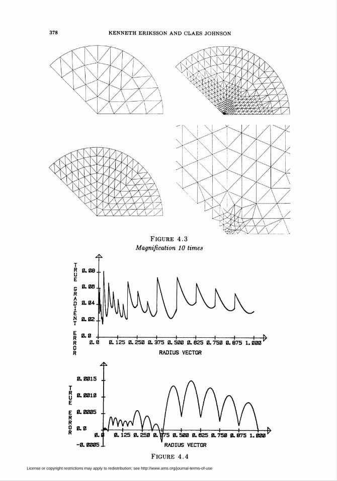
for the convex pie-shaped domain fi = {x = r(cos 0, sin 0) : 0 < r < 1, 0 < 0 <
3tt/4} with exact solution u(x) — r4/3 sin 40/3. In Figure 4.3 we give the sequence
of meshes produced by the algorithm with gradient control according to (4.1) with
8 = .1. In Figure 4.4 the actual gradient error |Ve(x)| and error |e(x)| are given
as functions of the distance |x| to the origin along the radius 0 = tt/2. We observe
that the gradient error is very well controlled, and thus the algorithm performs as
desired. We also note that the error |e(x)| decreases as x approaches the origin, as
is to be expected, since the mesh is overly refined with respect to control of HeHoo.n;
cf. Example 4.2 below.
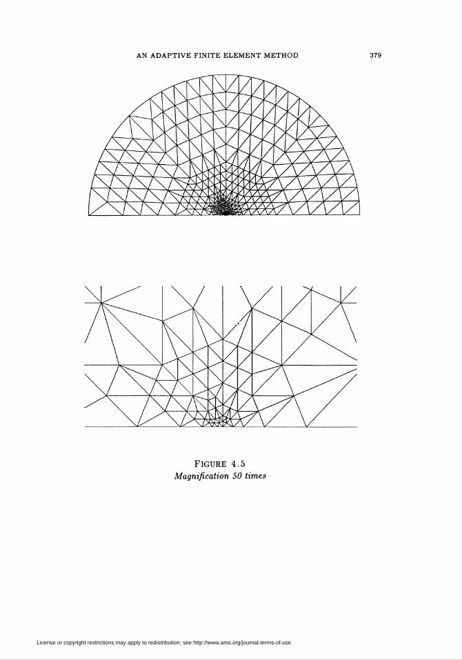
Example 4.2. To further illustrate the performance of the algorithm, we consider
the following mixed Dirichlet-Neumann problem
' Au = 0 in fi,
(4.3) , u = u0 onr|ur2,
du „— = 0 on Tj
v an
with exact solution u(x) = rxl2 sin 0/2, where fi is the semidisc {x: |x| < 1, x2 > 0}
with boundary T subdivided as follows: Vf = {x G T: xi ^ 0, X2 = 0}, T2 = {x G
T: X2 > 0}. In this case, u has a singularity of the form r0 with ß < 1, so that
Vu(x) is singular and |Ve(x)| —* oo as |x| —» 0 on any mesh.
License or copyright restrictions may apply to redistribution; see http://www.ams.org/journal-terms-of-use
378 KENNETH ERIKSSON AND CLAES JOHNSON
Figure 4.3Magnification 10 times
R0R
0.0 0. 125 0. 250 0. 375 0. 500 0. 625 0. 750 0. 875 1. 000
RADIUS VECTOR
0.0015 1
ERR0R 0.1
-0.0005..
0. 125 0. 250 0. 5 0.500 0.625 a 750 a 875 1.000
radius vector
Figure 4.4
License or copyright restrictions may apply to redistribution; see http://www.ams.org/journal-terms-of-use
AN ADAPTIVE FINITE ELEMENT METHOD 379
Figure 4.5Magnification 50 times
License or copyright restrictions may apply to redistribution; see http://www.ams.org/journal-terms-of-use
380 KENNETH ERIKSSON AND CLAES JOHNSON
TRUE
ERR0R
0.0020
0.0015
0.00101
0.0005
0.00.0 0. 125 0. 250 0. 375 0. 500 0. 625 0. 750 0. 875 1. 000
RADIUS VECTOR
0. 004
0.003
0.002
0. 001 1
0. 0000.0
-f- -f- -f- ~r- -I-
0.0050 0.0100 0.0150
RADIUS VECTOR
+~t
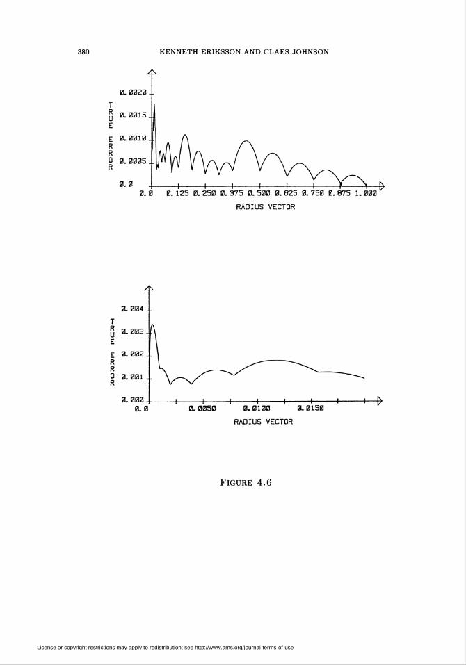
Figure 4.6
License or copyright restrictions may apply to redistribution; see http://www.ams.org/journal-terms-of-use
AN ADAPTIVE FINITE ELEMENT METHOD 381
m
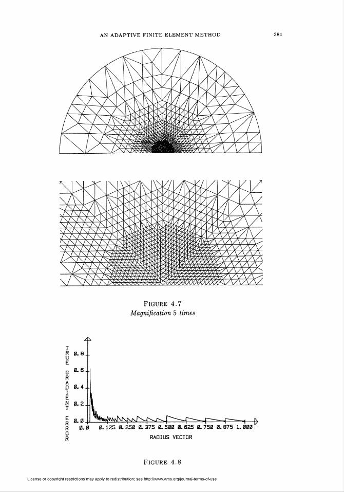
Figure 4.7
Magnification 5 times
TRUE
GRADIENT
ERR0R
0.8..
0.6..
0.4..
0-2.L
0.0
0.0 0.125 0.250 0.375 0.500 0.625 0.750 0.875 1.000
RADIUS VECTOR
Figure 4.8
License or copyright restrictions may apply to redistribution; see http://www.ams.org/journal-terms-of-use
382 KENNETH ERIKSSON AND CLAES JOHNSON
Let us now give the results obtained by applying our algorithm to this problem
with control of Hellen, that is, we simply replace hx and hk in (4.1) and (4.2) by
h2K and h2~. In Figure 4.5 we give the final mesh, with a zoom at the origin, obtained
starting with an initial mesh similar to the initial mesh in Figure 4.3 and using the
tolerance <5 = 0.01. We also give in Figure 4.6 the actual distribution of |e(x)| along
the same radius as above, again with a zoom. We observe that |e(x)| is roughly
constant in |x| and thus the algorithm succeeds in finding a well-equilibrated mesh.
A theoretical analysis and justification of the algorithm in the present case, which
is not covered by this note, since ß < 1, is given in [5].
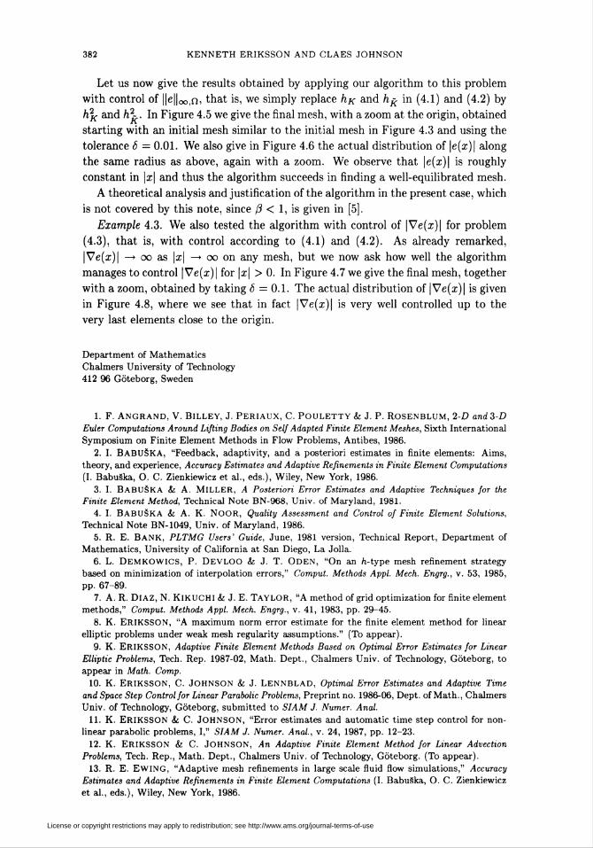
Example 4.3. We also tested the algorithm with control of |Ve(x)| for problem
(4.3), that is, with control according to (4.1) and (4.2). As already remarked,
|Ve(x)| —► oo as |x| —► oo on any mesh, but we now ask how well the algorithm
manages to control |Ve(x)| for |x| > 0. In Figure 4.7 we give the final mesh, together
with a zoom, obtained by taking 8 — 0.1. The actual distribution of |Ve(x)| is given
in Figure 4.8, where we see that in fact |Ve(x)| is very well controlled up to the
very last elements close to the origin.
Department of Mathematics
Chalmers University of Technology
412 96 Göteborg, Sweden
1. F. ANGRAND, V. BlLLEY, J. PERIAUX, C. POULETTY & J. P. ROSENBLUM, 2-D and 3-D
Euler Computations Around Lifting Bodies on Self Adapted Finite Element Meshes, Sixth International
Symposium on Finite Element Methods in Flow Problems, Antibes, 1986.
2. I. BabuSka, "Feedback, adaptivity, and a posteriori estimates in finite elements: Aims,
theory, and experience, Accuracy Estimates and Adaptive Refinements in Finite Element Computations
(I. Babuäka, O. C. Zienkiewicz et al., eds.), Wiley, New York, 1986.
3. I. BABUSKA & A. MILLER, A Posteriori Error Estimates and Adaptive Techniques for the
Finite Element Method, Technical Note BN-968, Univ. of Maryland, 1981.
4. I. BABUáKA & A. K. NOOR, Quality Assessment and Control of Finite Element Solutions,
Technical Note BN-1049, Univ. of Maryland, 1986.
5. R. E. BANK, PLTMG Users' Guide, June, 1981 version, Technical Report, Department of
Mathematics, University of California at San Diego, La Jolla.
6. L. DEMKOWICS, P. DEVLOO & J. T. ODEN, "On an /i-type mesh refinement strategy
based on minimization of interpolation errors," Comput. Methods Appl. Mech. Engrg., v. 53, 1985,
pp. 67-89.7. A. R. DIAZ, N. Kikuchi & J. E. TAYLOR, "A method of grid optimization for finite element
methods," Comput. Methods Appl. Mech. Engrg., v. 41, 1983, pp. 29-45.
8. K. ERIKSSON, "A maximum norm error estimate for the finite element method for linear
elliptic problems under weak mesh regularity assumptions." (To appear).
9. K. ERIKSSON, Adaptive Finite Element Methods Based on Optimal Error Estimates for Linear
Elliptic Problems, Tech. Rep. 1987-02, Math. Dept., Chalmers Univ. of Technology, Göteborg, to
appear in Math. Comp.
10. K. ERIKSSON, C. JOHNSON & J. Lennblad, Optimal Error Estimates and Adaptive Time
and Space Step Control for Linear Parabolic Problems, Preprint no. 1986-06, Dept. of Math., Chalmers
Univ. of Technology, Göteborg, submitted to SIAM J. Numer. Anal.
11. K. ERIKSSON & C. JOHNSON, "Error estimates and automatic time step control for non-
linear parabolic problems, I," SIAM J. Numer. Anal., v. 24, 1987, pp. 12-23.
12. K. ERIKSSON & C. JOHNSON, An Adaptive Finite Element Method for Linear Advection
Problems, Tech. Rep., Math. Dept., Chalmers Univ. of Technology, Göteborg. (To appear).
13. R. E. EWING, "Adaptive mesh refinements in large scale fluid flow simulations," Accuracy
Estimates and Adaptive Refinements in Finite Element Computations (I. BabuSka, O. C. Zienkiewicz
et al., eds.), Wiley, New York, 1986.
License or copyright restrictions may apply to redistribution; see http://www.ams.org/journal-terms-of-use
AN ADAPTIVE FINITE ELEMENT METHOD 383
14. C. JOHNSON, Error Estimates and Automatic Time Step Control for Numerical Methods for
Stiff Ordinary Differential Equations, Preprint no. 1984-27, Dept. of Math., Chalmers University of
Technology, Göteborg; revised version to appear in SIAM J. Numer. Anal.
15. C. JOHNSON, Y.-Y. NIE & V. THOMÉE, An A Posteriori Error Estimate and Automatic Time
Step Control for a Backward Euler Discretization of a Parabolic Problem, preprint no. 1985-23, Dept.
of Math., Chalmers University of Technology, Göteborg, submitted to SIAM J. Numer. Anal.
16. R. LOHNER, K. MORGAN & 0. C. ZIENKIEWICZ, "An adaptive finite element procedure
for compressible high speed flows," Comput. Methods Appl. Mech. Engrg., v. 51, 1985, pp. 441-465.
17. R. RANNACHER & R. SCOTT, "Some optimal error estimates for piecewise linear finite
element approximations," Math. Comp., v. 38, 1982, pp. 437-445.
18. A. H. SCHATZ & L. B. WAHLBIN, "Maximum norm estimates in the finite element method
on plane polynomial domains. Part 1," Math. Comp., v. 32, 1978, pp. 73-109.
19. A. H. SCHATZ & L. B. WAHLBIN, "Maximum norm estimates in the finite element method
on plane polygonal domains. Part 2, refinements," Math. Comp., v. 33, 1979, pp. 465-492.
License or copyright restrictions may apply to redistribution; see http://www.ams.org/journal-terms-of-use