ambient background model (abm): development of an urban gaussian dispersion model and its...

Atmospheric Environment Vol. 32, No. 11, pp. 1881—1891, 1998( 1998 Elsevier Science Ltd. All rights reserved

Printed in Great Britain1352—2310/98 $19.00#0.00PII: S1352–2310(97)00484–6

AMBIENT BACKGROUND MODEL (ABM): DEVELOPMENTOF AN URBAN GAUSSIAN DISPERSION MODEL AND ITS

APPLICATION TO LONDON

MANFRED SEIKA,-,‡ ROY M. HARRISON*,- and NORBERT METZ‡- Institute of Public and Environmental Health, University of Birmingham, Edgbaston,Birmingham B15 2TT, U.K.; and ‡ BMW AG, Department of Energy and Environment,

W-2, 80788 Munich, Germany

(First received 4 October 1996 and in final form 15 October 1997. Published May 1998)

Abstract—A Gaussian dispersion model called ABM (Ambient Background Model) has been developed forapplication within an urban air quality management model for the urban area of London. Hourlymeteorological data for the whole year are combined with a detailed gridded emission inventory, coveringtraffic and non-traffic point and area source emissions, to predict annual average air quality at a centralurban background monitoring site. The components NO

x, PM

10, C

6H

6, NMVOC and CO are calculated

within a modelling domain of 100 km by 100 km around the city. The impact of sources outside themodelling domain is estimated based on results from the EMEP European long-range model. The results ofthe modelling exercise are compared to measured ambient data at the central urban background siteLondon Bloomsbury for 1993. The comparisons show that the ABM model gives good predictions ofannual average concentrations, and is capable of modelling hourly fluctuations in air quality withacceptable results. ( 1998 Elsevier Science Ltd. All rights reserved

Key word index: Atmospheric dispersion model, urban air quality, London, urban air quality management.

NOTATION

Abbreviations

ABM Ambient Background ModelBLUME Berliner Luftguteme{netz (air quality

monitoring network)EMEP European long-range dispersion modelIMMAUS Name of a German dispersion modelLTS London Transport SurveyOECD Organization for Economic Co-operation and

DevelopmentQUARG Quality of Urban Air Review GroupSNAP Selected Nomenclature for Air PollutantsTA Luft Technische Anleitung Luft (German environ-

mental law—Air quality)VDI Verein Deutscher Ingenieure (Association of

German Engineers)

SNAP1. Selected Nomenclature of Air Pollutants, Tier 1

SNAP1 Description

1 Public power, cogeneration and district heat-ing plants

2 Commercial, institutional and residentialcombustion plants

3 Industrial combustion4 Production processes5 Extraction and distribution of fossil fuels

*Author to whom correspondence should be addressed.

6 Solvent use7 Road transport8 Other mobile sources and machinery9 Waste treatment and disposal

10 Agriculture11 Nature

INTRODUCTION

Atmospheric dispersion models are essential for anyair quality management exercise. A major impact ofpollutants such as NO

2, PM

10and benzene is their

local effect on human health and there is a needto predict how changes in emissions, resulting frompollution control policies, will contribute to meet-ing health-based air quality standards. The highestambient background concentrations of these localpollutants generally occur in the centre of major ur-ban areas which often coincide with the highest den-sity of human ‘‘receptors’’ present in the city.

Although short-term pollutant episodes such as theLondon smog in December 1991 (Bower et al., 1994)draw much public attention to local air quality issues,it is for many pollutants long-term ambient averagessuch as the annual mean and 98 percentile valuesthat are of major interest as air quality goals. Long-term ambient data are less dependent on extreme

1881

Fig. 1. Geometry of the standard dispersion field.

meteorological events and therefore better suited toproviding proper feedback for long-term planning.

As part of an air quality management project forLondon and Berlin an atmospheric dispersion modelhas been developed with the following capabilities: (1)To predict long-term background air quality for localpollutants at London Bloomsbury, a monitoring sitein the centre of London, (2) to analyse long-termambient data in terms of their emission sources andgeographical origins, (3) compatibility with Europeanmodelling exercises by covering an area of 4 OECDgrids as used by EMEP and CORINAIR, (4) easy touse in a normal PC environment, and (5) includinga high-speed option for its use in an overall air qualitymanagement model.

A Gaussian dispersion model called Ambient Back-ground Model (ABM) has been developed andapplied to the urban areas of London and Berlin. Thispaper presents a comparison of modelled againstmeasured data for 1993 at London Bloomsbury andgives some insights into the ABM model.

BACKGROUND

ABM is developed from a former dispersion modelcalled IMMAUS (Fath and Stern, 1989, 1991).IMMAUS was originally developed for former West-Berlin in 1989 by a company called GEOS GmbHwhich has close links to the Free University of Berlin.It has been used since then by the local environmentalagency in Berlin ‘‘Senatsverwaltung fu( r Stadtentwick-lung, ºmweltschutz und ¹echnologie’’ as part of theirwork on urban air quality management. The coredevelopment of IMMAUS took about 2 yr and in-volved various experts on dispersion modelling bothat the Free University of Berlin and the local environ-mental agency. A substantial amount of evaluationwork has been carried out using the air qualitymonitoring system BLUME in Berlin. Results of themodel are regularly published in the Berlin ‘‘Air Qual-ity Management Plan (¸uftreinhalteplan)’’ and areused to support strategic political decision makingwith regards to air quality management.

IMMAUS has been significantly further developedas part of our work and has been given a new name:ABM (Ambient Background Model). Several featureshave been added to IMMAUS and some procedureswere changed and updated. The components thathave been added are listed in the following section,marked by a dart. Besides the attachment of newcomponents, the changes involved (1) conversion ofthe model onto a new computer platform, (2) errorcorrection and (3) an extension and update of existingprocedures which included: (3a) Extending the stan-dard dispersion field from a width of 4 km to a max-imum of 15 km, (3b) applying the dry depositionmechanism to area sources, (3c) expansion from oneto four possible pollutants per model run (optiontransfer-matrix), (3d) including PM

10and benzene as

possible components, (3e) including new emission pat-terns such as cold start, evaporation and resuspendedroad dust, and (3f ) improved quality of meteorologi-cal input data due to an enhanced meteorologicalinput module.

From all the new developments and changes, it isthe calculation of the effective transport wind speeddue to plume rise and fall, that had the most signifi-cant impact on the model’s behaviour. This is espe-cially important, if the model is applied to large urbanareas.

DETAILED DESCRIPTION

The purpose of ABM is to analyse or predict an-nual mean background air quality at monitoring sitesin the centre of major urban areas. It consists of anarea source and a point source module. In the areasource module, one hundred virtual point sources,with an identical emission height, represent a 500 mby 500 m area source. Their impact on 20,000 virtualreceptors is stored in a so-called ‘‘standard dispersionfield’’ (see Fig. 1) according to a procedure by Stern(1975). The 20,000 virtual receptors cover a rectangleof 47.5 km by 4 km. To extend the original rectangu-lar standard dispersion field (IMMAUS) from a max-imum width of 4—15 km, the ABM model applies theprobability function of the standard normal distri-bution to the triangular remainder of the field(see Fig. 1).

The ABM model in its present configuration canhandle up to 8760 meteorological conditions, 32241]1 km grid area sources and 450 point sources. Aseach 1 km area source is simulated by 400 pointsources, the area source module is actually modellingup to 1.3 m point sources for 8760 meteorologicalconditions.

An overview of ABM’s main characteristics is listedbelow. Components that have been developed oradded as part of this study are marked by a filledsquare (j), while features that originate from theprevious Gaussian dispersion model are labelled bya filled diamond (r). Existing components that havebeen changed, updated or extended are markedblack (d).

1882 M. SEIKA et al.

Table 1. Dry deposition velocities v$

and wet deposition gradient j

NO2

NO C6H

6NMVOC PM

10CO

v$

in m s~1 0.0020 0.0015 0.0010 0.0010 0.0010 0j in s~1 4.25]10~5p0.6! 0 0 0 5]10~5 0

! p: Rainfall in mm h~1 (used dimensionless). In the case of nitrogen oxides, a fixedrelationship between NO and NO

2is assumed in the model. For London in 1993, 55% of

NOx

is assumed to be NO (in ppb).

f Components covered: NOx

(as NO2); Primary

PM10

; Benzene; NMVOC; CO.

(r) Gaussian plume dispersion including totalreflection (Fath and Stern, 1989).

(r) Chronological meteorological data, e.g. on anhourly basis (boundary layer depth, wind speed,wind direction, stability categories, cloudamount, temperature, sunrise, sunset and rain-fall).

f Dry and wet deposition. Dry deposition accordingto Chamberlain’s source depletion formulation(1953). The applied deposition velocities are givenin Table 1. Wet deposition, assuming an exponen-tial removal rate together with rainfall-dependentdeposition coefficients shown in Table 1.

(j) Calculation of the effective transport wind speeddue to plume rise or fall (see below).

(j) Boundary layer depth calculation (Thomson,1992).

(j) Transfer from the boundary layer into the freetroposphere (see below).

(j) Chemical removal of NO2

(see below).

f Stability category calculation using Klug/ Manierprocedure (TA Luft, 1986).

f Time, temperature and weather dependent break-down of annual to hourly emissions (see next sec-tion).

(r) Stability dependent vertical wind field exponentaccording to Vogt and Gei{ (1980), together withKlug/Manier stability categories.

(r) Stability and height dependent plume standarddeviation using McElroy and Pooler (1968), Vogtand Gei{ (1980) or Singer and Smith (1966) for-mulations (see below).

(r) Plume rise prediction for point sources (due tothe plume’s vertical impulse) according to theGerman VDI Richtlinie 3728 formulation (VDI,1982).

(j) Optional output of a transfer-matrix for itsefficient use in an air quality management model(see below).

(j) Option to simulate 10]10 km grid area sourcesas point sources according to Zanetti (1990).

(j) Optional consideration of the travel time betweenemission source and receptor for chronologicaldata output (considering the plume’s centre only).

The effective transport wind speed, uN , is an impor-tant variable within the Gaussian plume diffusionequation, as it is inversely proportional to themodelled concentration. The ABM model combinesthe measured wind speed u

!with its effective anemom-

eter height z!%&&

(not the real anemometer height z!),

and calculates the effective transport wind speedbased on the estimated height of the plume’s centreh#%/5

at the receptor (rather than the emission releaseheight h). The equation used is

uN "u!)A

h#%/5

z!%&&Bm

(1)

where u!is the wind speed at anemometer height z

!,

and z!%&&

is the effective height of the wind speedmeasurement, which is usually smaller than z

!. The

wind field exponent m is dependent on the stabilitycategory (Vogt and Gei{, 1980). It is assumed that,with an increasing distance from the source, the plumeis spreading throughout the boundary layer, and theactual height of the plume’s centre h

#%/5is steadily

approaching half the boundary layer depth H*. Equa-

tion (1), in combination with the applied wind fieldexponent m, is likely to overestimate the wind speedincrease at higher altitude. To compensate for thatmanner, the centre of the plume is assumed not to riseto more than 100 m (own estimate).

If the effective emission height h is below half theboundary layer depth H

*and h is smaller than 100 m,

equation (2) below is used to calculate h#%/5

. Thismethodology is similar to the one given by Doran andHorst (1985) which assume that h

#%/5equals 0.53 times

pzat the receptor. With point sources, it can be that

the effective emission height h is higher than half theboundary layer depth H

*(but smaller than 100 m or

H*). In this case, the height of the plume’s centre h

#%/5is

assumed to approach half the boundary layer depthH

*from above, and equation (3) is used.

h#%/5

"

pz

2#

h

2(2)

h#%/5

"Hi!A

pz

2#

Hi!h

2 B. (3)

Eq. (2) is applicable in the following case: If h#%/5

(hthen h

#%/5is set to h; If h

#%/5'0.5H

*then h

#%/5is set to

0.5H*; If h

#%/5'100 m then h

#%/5is set to 100 m. Eq. (3)

is used in the following case: If h#%/5

'h then h#%/5

is setto h; If h

#%/5(0.5H

*then h

#%/5is set to 0.5H

*.

Development of an urban Gaussian dispersion model 1883

As the effective transport wind speed is constantlychanging from the source to the receptor, it is neces-sary to calculate the real travel time of the plume’scentre t, which is used as an input for all depositionand removal processes. The following equations areused for that purpose:

t"distx

u41%#

; u41%#

"

:$*4590

uN dx

distxuN (4)

where distx is the distance between source and recep-tor, and u

41%#is the average wind speed (at the plume’s

centre) between source and receptor.For the transfer from the boundary layer into the

free troposphere, Chamberlain’s source depletionmodel is applied to the difference between the bound-ary layer depth H

*and the effective emission height h.

The entrainment loss velocity used is 0.015 m s~1

(own estimate).The conversion of NO

2to nitric acid is mainly

driven by the OH radical during daytime and byO

3at night. Both chemical reactions are assumed to

have an average exponential removal rate of 10% perhour (own estimate).

In terms of the applied plume standard deviations,McElroy and Pooler parameters are used for areasources, while for point sources, the plume spreadis logarithmically interpolated depending on theeffective emission height: McElroy and Pooler forheights below 50 m, Vogt and Gei{ at 100 m, andSinger and Smith above 150 m (Fath and Stern, 1991).

If the ABM model is used within an urban airquality management model, its output is a so-calledtransfer-matrix. A transfer-matrix describes the rela-tionship between emission sources and annual aver-age concentration at a given receptor for a specificmeteorological data set, emission pattern, and emis-sion height (e.g. exhaust emissions from London taxisat 2 m height, combined with one year of meteoro-logy). It is derived by setting every emission source toa standard source strength (e.g. 1 kt a~1 1 km~1 grid)and then run the dispersion model so that the annualaverage impact of each source on the receptor (e.g. themonitoring site London Bloomsbury) is stored separ-ately. The resulting source—receptor relationships areexpressed as annual average concentration per stan-dard source strength, e.g. (ngm~3)/(kt a~1).

Wind speeds below 1 m s~1 (at an effective height of10 m) are set to 1 m s~1 because the Gaussian plumediffusion equation cannot deal adequately with lowwind speeds. A test run of 3 yr of meteorological dataat Berlin Dahlem (1979, 1981, 1983) showed that, foran effective height of 10 m, this situation occurs inabout 3% of all cases.

In the case of inversions, the boundary layer depthcan be smaller than the effective emission height ofpoint sources. Therefore, if the effective emissionheight h of a point source is greater than 1.33 times theboundary layer depth H

*, the boundary layer depth is

changed to 1.1 times the effective emission height

h (Fath and Stern, 1991) and stable conditions areused for the dispersion (which means if the Klug andManier stability category is greater than 2, it is set to2). Should the effective emission height h be between1 and 1.33 times H

*, the boundary layer depth H

*is

changed to h (Fath and Stern, 1991).

APPLICATION TO THE URBAN AREA OF LONDON

The London modelling domain consists of 19101]1 km grids, 179 point sources and 75 10]10 kmgrids. Figure 2 shows how 1 km grids are surroundedby the 10 km network and how the whole modellingdomain fits into the European OECD grid network.The monitoring site London Bloomsbury, shown inthe centre of Fig. 2, is a central urban background sitewithin the U.K. Automatic Urban Network whoseobjective is to measure central urban backgroundconcentrations. Bloomsbury is a continuous and wellequipped site, operational since January 1992. Itmeasures NO, NO

2, PM

10, CO, SO

2, O

3, and since

1993 a number of VOCs.Hourly meteorological data from 1993 (8760 condi-

tions) have been combined with emission inventoriesfrom 1990 to 1993. The meteorological measurementsoriginate from the monitoring site at the LondonWeather Centre, which is about 2 km south ofLondon Bloomsbury. The wind speed anemometer isplaced on top of the Ministry of Defence building inWhitehall at a real height z

!of 35 m. The effective

anemometer height z! %&&

is estimated to be 22 m(personal communication, Meteorological Office,1996).

For the 1 km grid system and all point sourceswithin Greater London the following emission inven-tories have been used: (a) London Energy Study 1990(LRC, 1993), (b) road transport emission inventory for1993 using LTS traffic flow data for 1991 (MVA,1994a) combined with German UBA emission factorsfor 1993 (UBA, 1993a, b), and (c) estimates of smallarea source emissions which were not included in theLondon Energy study (Seika et al., 1996). Moredetailed information on the applied emission datais given by Seika (1996).

The resulting total emission inventory for GreaterLondon is shown in Table 2. Emission sources arecategorised into CORINAIR SNAP classificationgroups (see abbreviations). Road transport emissions(category 7) are made up of exhaust (EXH), cold start(CLD), gasoline particulate matter (GPM), high emit-ter (HE), negative air filter (NAF), running losses (RL),tyre wear and brake lining (TYR), evaporation (EVP)and hot soak (HOT) emissions. Emissions of the10 km grid system (and point sources outside GreaterLondon) originate from the national 1990 emissioninventory (Gillham et al., 1994). In the case of PM

10and CO, where no disaggregated emission data havebeen made available, top down estimates usingnational per capita emissions were made.


Fig. 2. ABM modelling domain—Greater London and its region.

Table 2. Emission inventory for Greater London 1993 in t a~1

SNAP1 NOx

PM10

C6H

6NMVOC CO

1 2292 205 6 607 1432 19165 583 16 1566 17733 6268 482 6 622 8154 0 0 0 0 05 0 0 644 8002 06 0 0 0 48746 07 69688 4584 4151 99804 4815808 15068 454 37 13098 1068149 0 0 0 0 0

10 0 0 0 0 011 0 0 0 3127 0Other! — 5690 — — —Total 112481 11998 4860 175572 591124

! Preliminary estimate of resuspended road dust emissions.

Time, temperature and weather dependencies areused to convert from annual to hourly emissions forthe following: Exhaust (XH..), cold start (CO..), evap-oration (EVAP), resuspended road dust (RD..), resi-dential combustion (HAUS), day and night (DAYN)and constant (CONS) emissions.

The breakdown for exhaust and cold start emis-sions is done for three vehicle groups, passenger cars(AU), heavy duty vehicles (HD) and taxis (TX). Forexhaust emissions an annual, weekly and diurnal vari-ation is taken into account; see Fig. 3. Multiplyingthese exhaust patterns with the corresponding diurnalvariation of cold starts (Fig. 4), and then weighting

them accordingly to ambient temperature (Table 3)gives the representative cold start emission patterns.Evaporative emissions are assumed to be temperaturedependent only. As with cold start emissions, equa-tion (5) is used together with the factors shown inTable 3.

*distr—fac"e5&!# >*T%.1 (5)

where * Temp is the actual minus average temper-ature in °C.

Resuspended road dust emissions are assumed tovary according to passenger car exhaust emissions


Fig. 3. Diurnal, weekly and annual traffic variation in London and estimated annual pattern of resusp-ended road dust emissions.

Fig. 4. Estimated diurnal variation (as a factor) of the percentage of starts being cold starts.

combined with the annual variation (RD) shown inFig. 3. Due to the higher coarse fraction of road dustemissions, an increased dry deposition velocity of0.01 m s~1, instead of 0.001 m s~1 for other PM

10emissions, is used for their dispersion. Furthermore,emissions are doubled if the average daily temper-ature is below 2°C (own estimate), to account for theexpected increase of salt usage on the road network.The ABM model also contains an option that allowsthe variation of road dust emissions if it is raining.

However, so far no clear correlation between rain androad dust could be identified and therefore this optionis not activated in this study. It should be noted thatall these variations do not affect the total sum ofemissions.

The emission pattern for residential combustion isdivided into hot water supply and house heating. It isassumed that 15% of the total emission is due to hotwater supply and does not vary throughout the year.The remaining 85% is assumed to occur only between


Table 3. Temperature dependence of exponent tfac

tfac in °C~1 NOx

NMVOC PM10

CO

Cold start! 0 !7.7% !2.5% !5.5%Evaporation" 0 6% 0 0

! Own estimates based on temperature dependence of coldstart emission factors in (UBA, 1993a).

"Own estimate. New modelling results suggest that thisfactor might be too small.

Fig. 5. Temperature- and time-dependent diurnal variation of residential combustion.

October and April (both inclusive) and to have a tem-perature- and time-dependent diurnal variation; seeFig. 5. A simplified estimate called day and night isused for activities that are generally more active dur-ing daytime than at night; see Fig. 6.

The combination of emission sources (per SNAPcategory) with the available emission patterns (for1 and 10 km area sources, and point sources) is shownin Table 4. The emission release height used fordispersion modelling is added in subscript to theemission pattern abbreviation.

In order to estimate the European impact on urbanair quality, the EMEP long-range model (Simpsonand Hov, 1990) has been applied to London Bloom-sbury for 1990. The necessary model runs were carriedout by the Norwegian Meteorological Institute andthe components covered were NO

x, NMHC and CO.

One model run was done including all EuropeanOECD emission grids, a second one excluding the4 OECD grids covered by the ABM modellingdomain (see Fig. 2). The resulting estimates for theEuropean background concentrations (due to emis-sions from outside the ABM model area) in 1990 and1993 are shown in Table 5. The figures for 1993 areused in this study.

To account for the local impact of emission sourceswithin a 500 m by 500 m area around London Blooms-

bury (which are not explicitly modelled), it is assumedthat their impact on total modelled air quality isaround 10% (own estimate). This estimate is later onreferred to as ‘‘local impact’’. The annual averageconcentration of secondary particles such asNH

4NO

3and (NH

4)2SO

4is assumed to be 12 kgm~3

derived by interpolation of the map of secondaryaerosol over the U.K. given by QUARG (1996).

RESULTS

A comparison of modelled against measured an-nual average concentrations is shown in Fig. 7. Themodelled long-term concentrations are within a rangeof $25% of the actual measurements. For the com-ponents NO

x, PM

10and benzene, the difference

between model prediction and measurement is lessthan 10%. Considering that there is a significant levelof uncertainty about the emissions data and theirdiurnal variation, these long-term results are con-sidered to be very good.

In order to analyse the model’s ability to predictmedium- and short-term variations in air quality,comparisons of average monthly and diurnal vari-ations of NO

xconcentrations are shown in Figs 8 and

9. The modelled concentrations include the Europeanbackground levels (see Table 5) but exclude the esti-mated local impact. Therefore, the modelled vari-ations are expected to be slightly below the measuredconcentrations. In the absence of more comprehensivedata, it had to be assumed that the annual averageEuropean background remains constant for all 8760hourly situations. The given emission variationconsiders all point and area sources within the onekilometre grid network.

Taking into account that short-term variations ofthe European background are not considered and


Fig. 6. Simplified diurnal variation of sources that are more active during daytime than at night.

Table 4. Combination of emission sources with diurnalemission patterns

SNAP1 1 km 10 km PS! SC 7" 1 km

1 — — CONS EXH XH..2#

2 HAUS15

CONS2

CONS CLD CO..2#

3 DAYN15

DAYN2

DAYN GPM XH..2#

4 DAYN15

DAYN2

— HE XH..2#

5 EVAP2

CONS2

CONS NAF XH..2#

6 EVAP10

DAYN2

— RL XH..2#

7 see SC 7 DAYN2

— TYR XH..2#

8 DAYN2

DAYN2

— EVP EVAP2

9 CONS2

CONS2

CONS HOT XHAU2

10 CONS2

CONS2

— Other 1 km11 CONS

10CONS

2— RD RDAU

2

! Point sources."SNAP category 7: Road transport.# AU is used for passenger cars and light duty vehicles, HD

for HDVs and buses and TX for taxis.

Table 5. Estimate of European background concentrations at LondonBloomsbury in lgm~3 annual mean

NOx! Primary PM

10C

6H

6NMVOC" CO

1990# 13.7 22 2781993$ 15.4 1.8% 1.3& 22 186

! (as NO2).

"Conversion ppbC to lgm~3 using national emission sourcecategory split of 1990.

# EMEP model results.$Own estimates for 1993 based on relationship between annual

average air quality at London Bloomsbury in 1993 and 1990.% Assuming similar behaviour for primary PM

10than for NO

x.

Average secondary PM10

is assumed to be 12 lgm~3.& Assuming that the European background of benzene (as a percent-

age of the measured 1993 concentration at London Bloomsbury) isproportionally higher than for NO

xbut lower than for CO (average of

both is used).

that the local impact is also neglected, the model givesgood predictions. However, the diurnal variationseems to indicate that the ABM model is over-predict-ing the morning peak and under-predicting the mid-day period. So far two explanations seem plausible forthis phenomenon: (a) It seems possible that the InputModule, which is used for calculating boundary layerdepths, is on average over-predicting the height of theboundary layer for the midday period, and (b) it couldbe related to the way the Gaussian approach is deal-ing with varying wind speeds. Comparisons of meas-ured against modelled boundary layer depths inBerlin showed that, over a period of three years, theInput Module is likely to over-predict the mixingheight for the midday period by about 35%. Thecomparison was made for all days in 1979, 1981 and1983 using radio-sonde measurements of the temper-ature inversion found at Tegel airport. The measured


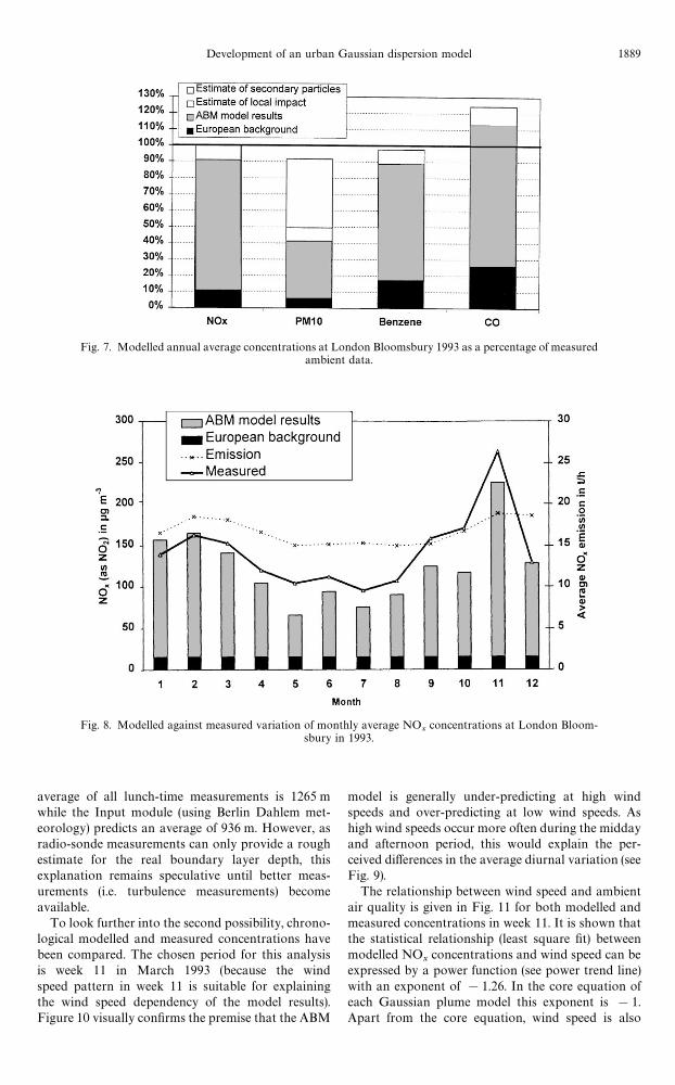
Fig. 7. Modelled annual average concentrations at London Bloomsbury 1993 as a percentage of measuredambient data.

Fig. 8. Modelled against measured variation of monthly average NOx

concentrations at London Bloom-sbury in 1993.

average of all lunch-time measurements is 1265 mwhile the Input module (using Berlin Dahlem met-eorology) predicts an average of 936 m. However, asradio-sonde measurements can only provide a roughestimate for the real boundary layer depth, thisexplanation remains speculative until better meas-urements (i.e. turbulence measurements) becomeavailable.

To look further into the second possibility, chrono-logical modelled and measured concentrations havebeen compared. The chosen period for this analysisis week 11 in March 1993 (because the windspeed pattern in week 11 is suitable for explainingthe wind speed dependency of the model results).Figure 10 visually confirms the premise that the ABM

model is generally under-predicting at high windspeeds and over-predicting at low wind speeds. Ashigh wind speeds occur more often during the middayand afternoon period, this would explain the per-ceived differences in the average diurnal variation (seeFig. 9).

The relationship between wind speed and ambientair quality is given in Fig. 11 for both modelled andmeasured concentrations in week 11. It is shown thatthe statistical relationship (least square fit) betweenmodelled NO

xconcentrations and wind speed can be

expressed by a power function (see power trend line)with an exponent of !1.26. In the core equation ofeach Gaussian plume model this exponent is !1.Apart from the core equation, wind speed is also


Fig. 9. Modelled against measured average diurnal variation of NOx

concentrations at London Bloom-sbury in 1993.

Fig. 10. Modelled against measured chronological air quality data for week 11, March 1993.

influencing the calculation of the atmospheric stabil-ity and the boundary layer depth in a way that helpsto decrease the above-mentioned exponent. There-fore, from a modelling point of view, the given expo-nent of !1.26 appears quite plausible. The fact thatthe measured values have an exponent above !1may indicate a more general problem of Gaussianplume models and the way they are dealing withvarying wind speeds.

CONCLUSIONS

The comparisons show that the ABM model givesremarkably good predictions of long-term urban

background air quality. Even when comparingmodelled against measured medium- and short-termconcentrations, it still performs well. Therefore, theABM model is suitable for the purpose of analysinglong-term urban background concentrations in termsof the responsible emission sources and their geo-graphical location. Areas where improvements maybe needed appear to be connected with the way theGaussian approach deals with varying wind speedsand possibly the way the applied meteorological inputmodule calculates midday boundary layer depths.

Acknowledgements—The authors would like to thank thefollowing organisations for the provision of data: Meteoro-logical Office; GEOS GmbH, Berlin; AEA - NETCEN; The


Fig. 11. Relationship between wind speed and ambient (modelled and measured) NOx

concentrations.

Norwegian Meteorological Institute; Government Office forLondon; MVA Consultancy; London Research Centre;Department of Transport. Helpful discussions with DavidThomson, Meteorological Office, Mr. Lenschow and Mr.Reichenbacher, Senatsverwaltung SUT Berlin, AndreasSkouloudis, JRC-Ispra, Robert Ireson, Systems ApplicationInternational, and David Simpson, The Norwegian Me-teorological Institute are very much appreciated. Specialthanks to Mr. Scherer and Mr. Fath, GEOS GmbH forsupplying the former IMMAUS model and their willingnessto answer a rather huge number of questions at the begin-ning of this project.

REFERENCES

Bower, J. S., Broughton, J. R., Stedman and Williams, M. L.(1994) A winter smog episode in the U.K. AtmosphericEnvironment 28, 461—476.

Doran, J. C. and Horst, T. W. (1985) An evaluation ofGaussian plume-depletion models with dual-tracer fieldmeasurements, Atmospheric Environment 19, 939—951.

Fath, J. and Stern, R. (1989) Ein immissionsklimatologischesAusbreitungsmodell auf der Basis der Gauss’schenPlume-Gleichung—Modellbeschreibungund Benutzeran-leitung. GEOS, Berlin.

Fath, J. and Stern, R. (1991) Verursacherspezifische Aus-breitungsrechnungen fur die Region Berlin. GEOS; Berlin.

Gillham, C., Couling, S., Leech, P. and Eggleston, H. (1994)National Atmospheric Emission Inventory—º.K. Emis-sions of Air Pollutants 1970—1991, LR 961, Warren SpringLaboratory, Stevenage; ISBN 0-85624-821-5.

LRC (1993) Hutchinson, D. and Chell, M., ¸ondon EnergyStudy—Energy ºse and the Environment; LondonResearch Centre, London, ISBN: 185261188.

McElroy, J. L. and Pooler, F. (1968) St. Louis dispersionstudy. U.S. Public Health Service, National Air PollutionControl Administration, Report AP-53.

QUARG (1996) Airborne Particulate Matter in the UnitedKingdom. Third report of the Quality of Urban AirReview Group. DOE, London, ISBN 0-9520771-3-2.

Seika, M. (1996) Evaluation of control strategies for improv-ing urban air quality with London and Berlin as examples.

Ph.D. study, Institute of Public and EnvironmentalHealth, University of Birmingham.

Seika, M., Metz, N. and Harrison, R. M. (1996) Character-istics of urban and state emission inventories—A compari-son of examples from Europe and the United States; TheScience of the Total Environment, 189, 221—234, ISSN0048-9697.

Singer, I. A. and Smith, M. E. (1966) Atmospheric dispersionat Brookhaven National Laboratory, Air ¼ater PollutionInternational 10, 125—135.

Simpson, D. and Hov, ". (1990) Long period modelling ofphotochemical oxidants in Europe—Calculations for July1985. EMEP MSC-W Note 2/90, Norwegian Meteoro-logical Institute, Oslo.

Stern, R. (1975) Modell- und Programmbeschreibungdes Fortak’schen Viel-Quellen-Diffusions-Modells. In-stitut fur theoretische Meteorologie der Freien Univer-sitat, Berlin.

TA Luft (1986) Erste allgemeine Verwaltungsvorschrift zumBundes-Immissions-Schutz-Gesetz-Technische Anleitungzur Reinhaltung der Luft - TA Luft vom 27, February1986.

Thomson, D. (1992) The Met Input Module, UK ADMS 1.0,Internal paper, Meteorological Office, Bracknell

UBA (1993a) Hassel, D. et al., Abgas-Emissionsfaktoren vonPkw in der Bundesrepublik Deutschland—Abgasemis-sionen von Fahrzeugen der Baujahre 86 bis 90. UBA-FB91-042, Umweltbundesamt, Berlin

UBA (1993b) Hassel, D. et al., Abgas-Emissionsfaktoren vonNutzfahrzeugen in der Bundesrepublik Deutschland furdas Bezugsjahr 1990. Umweltbundesamt, Berlin

VDI (1982) VDI Richtlinien—Ausbreitung von Luftverun-reinigungen in der Atmosphare—Ausbreitungs-modell furLuftreinhalteplane. VDI 3782 Blatt 1, Grundruck.

Vogt, K. and Gei{, H. (1980) Neue Ausbreitungskoeffizien-ten fur 50 und 100 m Emissionshohe. -80 (458) SSK/S4—39/U3 (literature reference taken from Fath and Stern,1989).

Wang (1996) Determination of transport wind speed in theGaussian plume diffusion equation for low-lying pointsources, Atmospheric Environment 30, 661—665.

Zanetti, P. (1990) Air Pollution Modelling: ¹heories, Com-putational Methods and Available Software. Van NostrandReinhold, New York.


ambient background model (abm): development of an urban gaussian dispersion model and its...

Documents