am-fm - university of texas at...
TRANSCRIPT
AM-FM Image Models
Joseph P. Havlicek
Laboratory for Vision Systems
Center for Vision and Image Sciences
The University of Texas
Austin, TX 78712-1084
USA
November 8, 1996

GOAL
� MODEL images as sums of AM-FM functions:
t(m) =KXi=1
ai(m) exp[j'i(m)]:
� ESTIMATE the dominant image modulations.
� COMPUTE multi-component AM-FM image
representations.
� RECOVER the essential image structure from the
computed representations.

OUTLINE
I.Introduction
II. Demodulation
III. Dominant Component Analysis
IV. Multi-Component Analysis
V. Conclusions
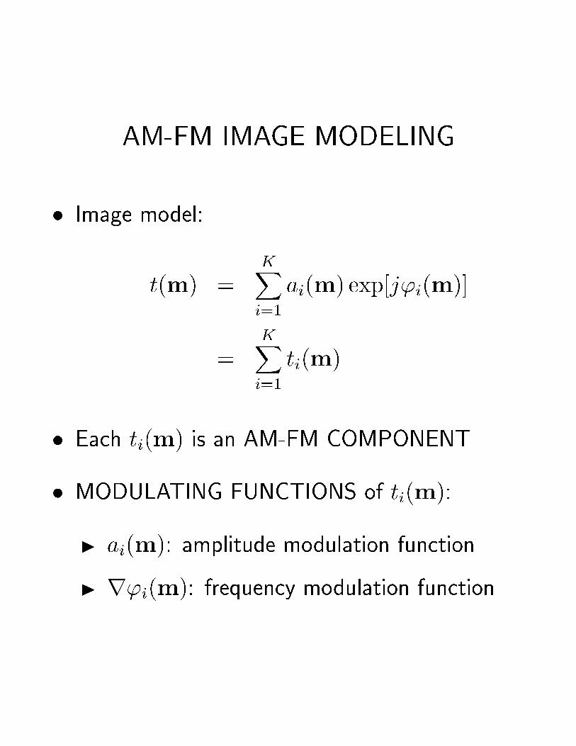
AM-FM IMAGE MODELING
� Image model:
t(m) =KXi=1
ai(m) exp[j'i(m)]
=KXi=1
ti(m)
� Each ti(m) is an AM-FM COMPONENT.
� MODULATING FUNCTIONS of ti(m):
I ai(m): amplitude modulation function.
I r'i(m): frequency modulation function.

COMPARISON TO DFT
� DFT represents an N �N image as the sum of
N 2sinusoidal components, each having
I constant amplitude.
I constant frequency.
� Nonstationary structure represented by construc-
tive and destructive INTERFERENCE between
STATIONARY components.
� The modulating functions ai(m) and r'i(m)
are permitted to vary smoothly across the image.
� EACH AM-FM component is capable of capturing
SIGNIFICANT nonstationary structure.
� AM-FM model captures essential image structure
using MUCH fewer than N 2components.
1D BACKGROUND
� In 1977, Moorer
I COMPUTED multi-component AM-FM rep-
resentations for musical instrument signals.
I CODED the representations and achieved
compression ratios of 43:1.
I RECONSTRUCTED the signals from the
computed representations.
I Assumed harmonically related components.
� 1D Teager-Kaiser operator introduced in 1990.
� Energy Separation Algorithm (ESA) developed by
Maragos, Kaiser, & Quatieri (1991).
I Used by MANY people for AM-FM speech
modeling.

1D MULTI-COMPONENT MODELS
� Kumaresan, Sadasiv, Ramalingam, and Kaiser
(1992-96):
I Used Teager-Kaiser operator and matrix
invariance properties.
I Problems with K > 4 components.
I Problems with n > 1 dimensions.
� Lu and Doerschuck (1996).
I Used Kalman �lters.
I 1D formulation.
2D BACKGROUND
� Bovik, Clark, & Geisler characterized TEXTURE
as a CARRIER of region information (1986).
I MODELED textures as single-component
AM-FM functions.
I SEGMENTED texture using amplitude and
phase of Gabor �lter response.
� Bovik, et. al., estimated DOMINANT modulating
functions via an iterative relaxation algorithm
(1992).
I SEGMENTED textures.
I RECONSTRUCTED 3D surfaces.
I Iteration was computationally EXPENSIVE.
2D AM-FM MODELS
� Knutsson, Westin, & Granlund (1994).
I Used lognormal �lters.
I Estimated FM for a single component.
� Francos and Friedlander (1995-96).
I Polynomial phase model.
I Estimated polynomial order and coe�cients.
I Demonstrated on simple synthetics.
2D TEAGER-KAISER OPERATOR
� Introduced by Yu, Mitra, & Kaiser (1991).
� 2D ESA: Maragos, Bovik, & Quatieri (1992).
I Computationally e�cient.
I Promised to replace iterative relaxation tech-
nique for estimating dominant modulations.
� Havlicek began work on the problem (1992).
� TROUBLE:
I ESA cannot estimate SIGNED frequency.
I SIGN of frequency is important in multi-D:
embodies ORIENTATION.
� A NEW approach was needed.
� Slides Here
1. reptile
2. reptile baseband comp, comp 1
3. reptile comp 2, comp 3
4. reptile
5. reptile comp 4, comp 5
I look at how \fold" is in FM of comps 2, 3.
Also in AM of baseband and comps 4, 5.
Comp 1 is AM-FM harmonic of comp 3.
6. All six reptile components.
7. reptile + 6 comp recon
8. reptile + 43 channelized comp recon

SIGNIFICANCE
� These results are AMAZING!!
� FIRST approach to
I Estimate multi-D multi-component amplitude
and frequency modulations.
I Estimate multi-D multi-component FM with
CORRECT signs.
I Compute multi-component AM-FM represen-
tations for natural images.
I Reconstruct from estimated modulations (in
both 1D & 2D).

APPLICATIONS
� Texture-based scene segmentation. (Bovik, Clark,
Geisler; Porat, Zeevi; Havlicek, Harding, Bovik)
� Phase-based computational stereopsis. (Chen,
Bovik).
� 3-D shape from texture. (Super, Bovik,
Klarquist).

APPLICATIONS: : :
� Spatio-spectral analysis.
� Texture modeling and synthesis.
� Future:
I Image coding.
I Video coding.
I Multimedia and CD-ROM applications.

OUTLINE
I. Introduction
II.Demodulation
III. Dominant Component Analysis
IV. Multi-Component Analysis
V. Conclusions
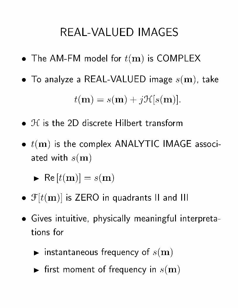
REAL-VALUED IMAGES
� The AM-FM model for t(m) is COMPLEX.
� To analyze a REAL-VALUED image s(m), take
t(m) = s(m) + jH[s(m)]:
� H is the 2D discrete Hilbert transform.
� t(m) is the complex ANALYTIC IMAGE associ-
ated with s(m).
I Re [t(m)] = s(m).
� F[t(m)] is ZERO in quadrants II and III.
� Gives intuitive, physically meaningful interpreta-
tions for
I instantaneous frequency of s(m).
I �rst moment of frequency in s(m).

DEMODULATION
� Demodulation algorithm is NONLINEAR.
� Cross-component interference is a PROBLEM if
t(m) is MULTI-COMPONENT.
� Use a multiband bank of linear �lters gp(m) to
ISOLATE components on a POINTWISE basis.
I The �lters DO NOT need to isolate the
components on a GLOBAL scale.
I The response yp(m) of each �lter gp(m)
DOES need to be dominated by only ONE
component at each image pixel.
� Suppose that component ti(m) dominates the
response yp(m) of �lter gp(m) at pixel m.
� GOAL: use the response yp(m) to estimate the
values of the modulating functions ai(m) and
r'i(m) at pixel m.

DEMODULATION: : :
� Demodulation algorithm depends on a quasi-
eigenfunction approximation (QEA).
� Suppose Gp is a 2D LSI system.
� Exact response to ti(m):
yp(m) =Xp2Z2
gp(p)ti(m� p):
� QEA:
byp(m) = ti(m)Gp[r'i(m)]:
� QEA error generally small or negligible if
I gp(m) spatially localized.
I ai(m) and r'i(m) are smoothly varying, or
LOCALLY COHERENT.
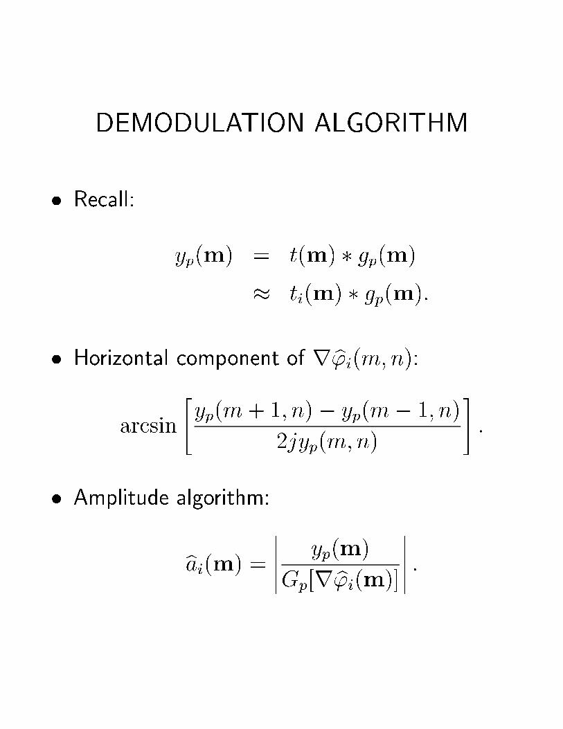
DEMODULATION ALGORITHM
� Recall:
yp(m) = t(m) � gp(m)
� ti(m) � gp(m):
� Horizontal component of r b'i(m;n):
arcsin
"yp(m+ 1; n)� yp(m� 1; n)
2jyp(m;n)
#:
� Amplitude algorithm:
bai(m) =
����� yp(m)
Gp[r b'i(m)]
����� :

FILTERBANK
� Physiology and psychophysics:
I CHANNELS in visual cortex operate at 18
orientations and 4 magnitude frequencies.
I Visual cortical cells function as 2D complex
Gabor �lters.
� For ANALYTIC images t(m), only half of the
orientations need be considered.
� 2D Gabor �lters have OPTIMAL spatio-spectral
localization.
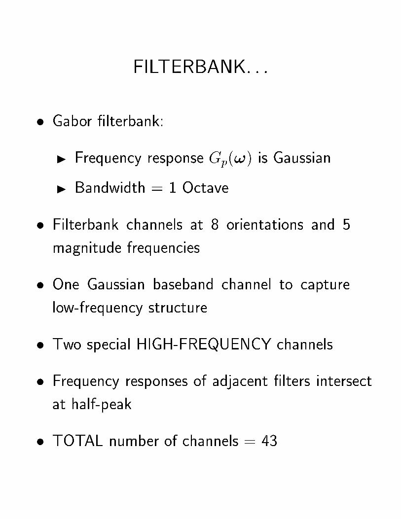
FILTERBANK: : :
� Gabor �lterbank:
I Frequency response Gp(!) is Gaussian.
I Bandwidth = 1 Octave.
� Filterbank channels at 8 orientations and 5
magnitude frequencies.
� One Gaussian baseband channel to capture
low-frequency structure.
� Two special HIGH-FREQUENCY channels.
� Frequency responses of adjacent �lters intersect
at half-peak.
� TOTAL number of channels = 43.
� Slides Here
9. Filterbank in frequency domain.
OUTLINE
I. Introduction
II. Demodulation
III.
Dominant Component Analysis
IV. Multi-Component Analysis
V. Conclusions
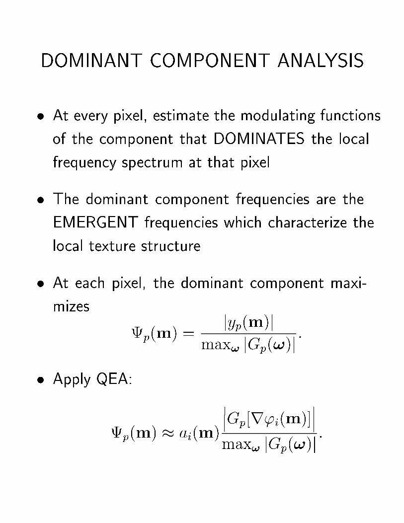
DOMINANT COMPONENT ANALYSIS
� At every pixel, estimate the modulating functions
of the component that DOMINATES the local
frequency spectrum at that pixel.
� The dominant component frequencies are the
EMERGENT frequencies which characterize the
local texture structure.
� At each pixel, the dominant component maxi-
mizes
p(m) =jyp(m)j
max! jGp(!)j:
� Apply QEA:
p(m) � ai(m)
���Gp[r'i(m)]���
max! jGp(!)j:

BLOCK DIAGRAM
t(m)
ESA
ESA
ESA
1
2
G
G
GM
ϕ
ϕ
ϕ
a
a
a
1 / Gmax
1 / Gmax
1 / Gmax
ChannelSelectMax
^
^
^
^
^
^

� Slides Here
10. Tree + dom comp recon
11. Ra�a + dom comp recon
12. Burlap + dom recon

TEXTURE SEGMENTATION
� Apply LoG edge detector to dominant
I Frequency magnitudes.
I Frequency orientations.
I Amplitudes.
� Segment along SIGNIFICANT zero crossings.

� Slides Here
13. MicaBurlap Mag Freq + Seg, � = 15, � = 1:5
PelletBean Mag Freq + Seg, � = 49, No �
14. WoodWood Arg Freq + Seg, � = 14, � = 11
PaperBurlap AM + Seg, � = 46:5, No �

APPLICATIONS
� Spatio-spectral analysis.
� Image segmentation.
� Phase-based stereo (Chen, Bovik).
� 3-D shape from texture (Super, Bovik,
Klarquist).
� Biologically feasible model of mammalian visual
function.
OUTLINE
I. Introduction
II. Demodulation
III. Dominant Component Analysis
IV.
Multi-Component Analysis
V. Conclusions
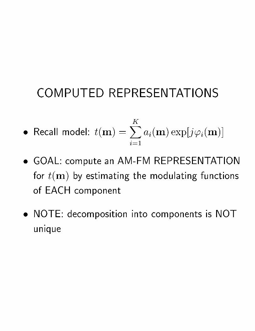
COMPUTED REPRESENTATIONS
� Recall model: t(m) =KXi=1
ai(m) exp[j'i(m)].
� GOAL: compute an AM-FM REPRESENTATION
for t(m) by estimating the modulating functions
of EACH component.
� NOTE: decomposition into components is NOT
unique.

CHANNELIZED COMPONENTS
� Estimate modulating functions for ONE compo-
nent from EACH �lterbank channel.
� M -channel �lterbank ) M -component represen-
tation.
� Consistent with biological vision models.
� Gives good reconstructions.
� Slides Here
15. reptile + recon (channelized comps)
16. ra�a + recon (channelized comps)
17. tree + recon (channelized comps)
18. pebbles + recon (channelized comps)
19. Ocean City, NJ + recon (channelized comps)
20. Celebrity + recon (channelized comps)

CHANNELIZED COMPONENTS: : :
� NOT EFFICIENT:
I Many images have FEWER than M compo-
nents.
I Often, many components are nearly zero over
large regions.
I Single elements of the image structure tend
to be manifest in more than one channelized
component.
� SHOULD be able to get BETTER results with
FEWER components.
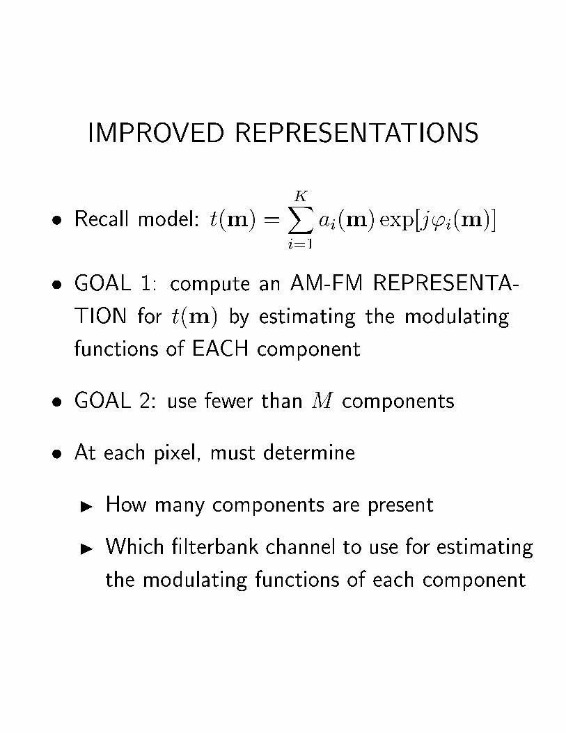
IMPROVED REPRESENTATIONS
� Recall model: t(m) =KXi=1
ai(m) exp[j'i(m)].
� GOAL 1: compute an AM-FM REPRESENTA-
TION for t(m) by estimating the modulating
functions of EACH component.
� GOAL 2: use fewer than M components.
� At each pixel, must determine
I How many components are present.
I Which �lterbank channel to use for estimating
the modulating functions of each component.
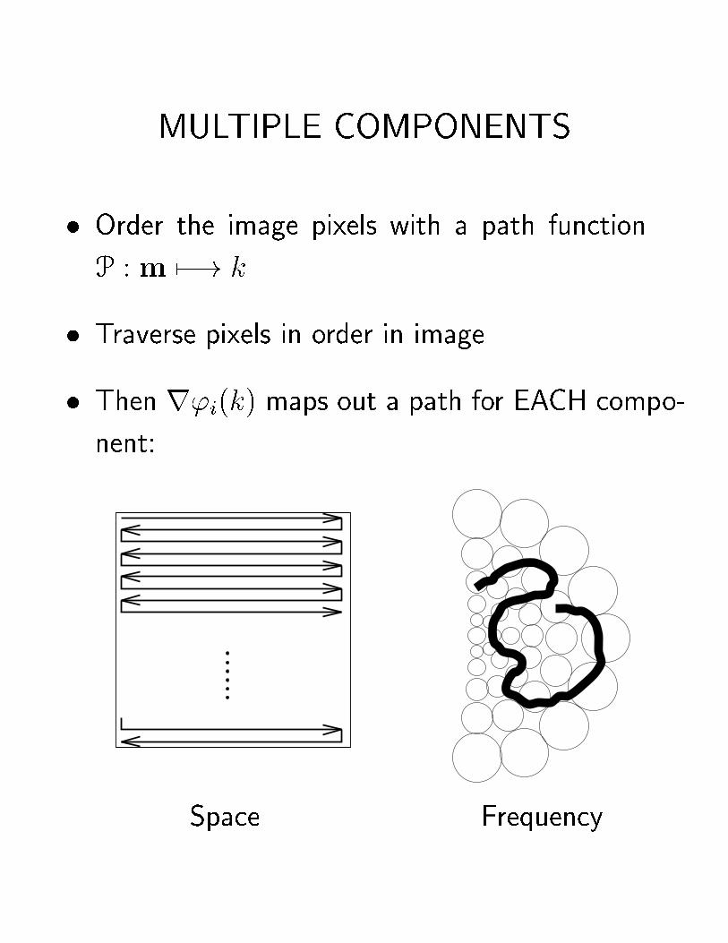
MULTIPLE COMPONENTS
� Order the image pixels with a path function
P :m 7�! k.
� Traverse pixels in order in image.
� Then r'i(k) maps out a path for EACH compo-
nent:
Space Frequency

TRACK PROCESSOR
� Expand modulating functions of ti(m) in Taylor
series to obtain a canonical state-space model.
� Model higher-order derivatives of modulating
functions AND errors in bai(m) and r b'i(m) as
STOCHASTIC PROCESSES.
� Use a Kalman �lter to track the modulating
functions of each component across the �lterbank
channel responses.
I INPUTS the estimated modulating functions
computed from the CHANNEL responses.
I PREDICTS which channel should be used for
estimating the modulating functions of each
component.
I OUTPUTS estimated modulating functions
for each COMPONENT.

BLOCK DIAGRAM
ϕ
ϕ
ϕ
ϕ
ϕ
ϕ
ϕ
t(m) Track
Processor
ESA
ESA
3 ESA
ESA
1
2
a
a
a
a
a
aK
1a
2
G
G
G
MG
1
2
K
^
^
^
^
^
^
^
^
~
~
~
~
~
~

THE NEED FOR POSTFILTERING
� PROBLEM: image phase discontinuities cause
I Abrupt, large-scale excursions in r'i(m).
I Nontrivial QEA errors.
I Absurd amplitude estimates.
� Frequency excursions can be UNBOUNDED.
� If the track processor follows a frequency excur-
sion in ti(m), it
I Rapidly updates from MANY channels.
I Often updates from a channel that is domi-
nated by another component.
I The track of ti(m) is then lost.
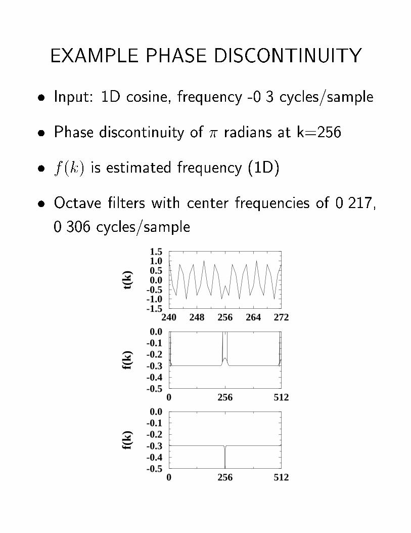
EXAMPLE PHASE DISCONTINUITY
� Input: 1D cosine, frequency -0.3 cycles/sample.
� Phase discontinuity of � radians at k=256.
� f(k) is estimated frequency (1D).
� Octave �lters with center frequencies of 0.217,
0.306 cycles/sample
0 256 512-0.5-0.4-0.3-0.2-0.10.0
f(k)
0 256 512-0.5-0.4-0.3-0.2-0.10.0
f(k)
240 248 256 264 272-1.5-1.0-0.50.00.51.01.5
t(k)

POSTFILTERS
� Natural images are expected to contain phase
discontinuities:
I Occlusions.
I Surface discontinuities, defects, deformations.
I Shadows and specularities.
I Noise.
� SOLUTION: Post-process the estimated modulat-
ing functions delivered by gp(m) with a low-pass
Gaussian smoothing �lter Pp(!).
� Post�ltered channel model:
AMP
FREQALG
ALG p a
ϕ^ t(m) Gp Pp
P
� Slides Here
21. reptile + recon (baseband + 5 tracked comps)
22. straw + recon (baseband + 8 tracked comps)
23. recons of 2 tracked straw comps
24. recons of 2 tracked straw comps
25. pellets + recon (baseband + 12 tracked
comps)
26. recons of 2 tracked pellets comps
27. recons of 2 tracked pellets comps
28. burlap + recon (baseband + 8 tracked comps)
29. recons of 2 tracked burlap comps
30. ra�a + recon (baseband + 8 tracked comps)
31. ice + recon (baseband + 12 tracked comps)
APPLICATIONS
� Nonstationary spatio-spectral analysis.
� Image and video coding.
� Current track processor has di�culty with
I Regionally supported structure
I images containing multiple textured objects.
� Investigation of IMPROVED tracking approaches
is ongoing.

OUTLINE
I. Introduction
II. Demodulation
III. Dominant Component Analysis
IV. Multi-Component Analysis
V.Conclusions

CONTRIBUTION
� Developed a NEW theory of multidimensional
AM-FM signal modeling.
I Applicable in ARBITRARY dimensions.
I Continuous AND discrete theories.
� FIRST to:
I estimate multi-D multi-component AM-FM.
I estimate multi-D FM with CORRECT signs.
I comprehensively treat multi-D analytic signal.
I treat multi-D QEA theory.
� Developed two computational paradigms in 2D.
FIRST to:
I compute multi-component AM-FM represen-
tations for natural images.
I reconstruct from estimated modulations (in
both 1D & 2D).
CONCLUSIONS
� Estimated dominant image modulations.
� Computed AM-FM representations.
� Reconstructed from the representations.
� USEFUL in PRACTICAL engineering systems:
I Texture segmentation.
I Phase based computational stereopsis.
I 3D shape from texture.
I Spatio-spectral analysis.
� Future work:
I Improved tracking approaches.
I Color images.
I Video and color video.
I Image and video coding.
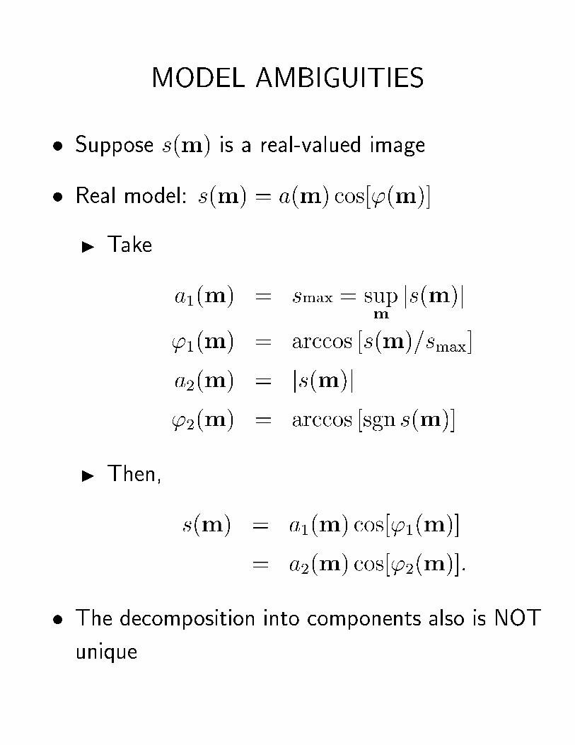
MODEL AMBIGUITIES
� Suppose s(m) is a real-valued image.
� Real model: s(m) = a(m) cos['(m)].
I Take
a1(m) = smax = supmjs(m)j
'1(m) = arccos [s(m)=smax]
a2(m) = js(m)j
'2(m) = arccos [sgn s(m)]
I Then,
s(m) = a1(m) cos['1(m)]
= a2(m) cos['2(m)]:
� The decomposition into components also is NOT
unique.
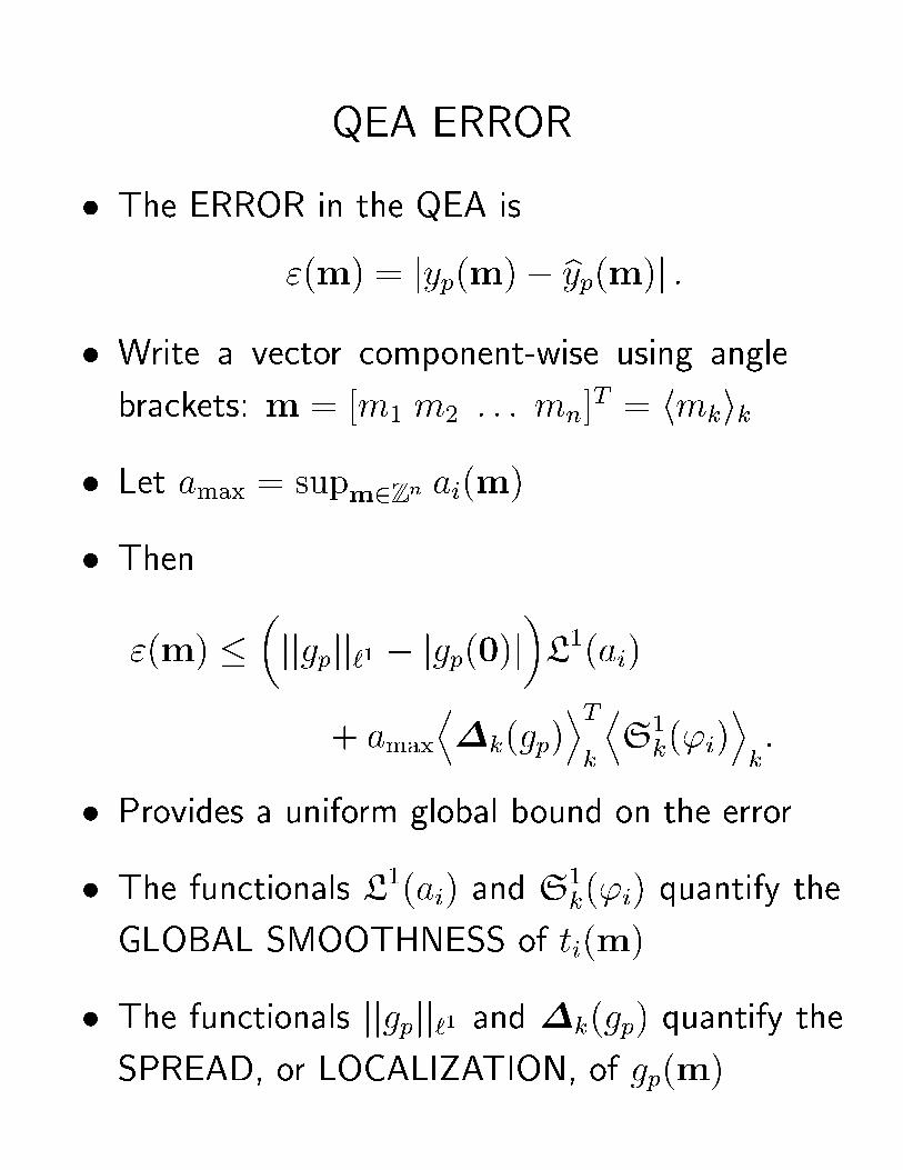
QEA ERROR
� The ERROR in the QEA is
"(m) = jyp(m)� byp(m)j :
� Write a vector component-wise using angle
brackets: m = [m1 m2 : : : mn]T = hmkik.
� Let amax = supm2Zn ai(m).
� Then
"(m) �
�jjgpjj`1 � jgp(0)j
�L1(ai)
+ amaxD�k(gp)
ETk
DS
1k('i)
Ek:
� Provides a uniform global bound on the error.
� The functionals L1(ai) and S
1k('i) quantify the
GLOBAL SMOOTHNESS of ti(m).
� The functionals jjgpjj`1 and �k(gp) quantify the
SPREAD, or LOCALIZATION, of gp(m).
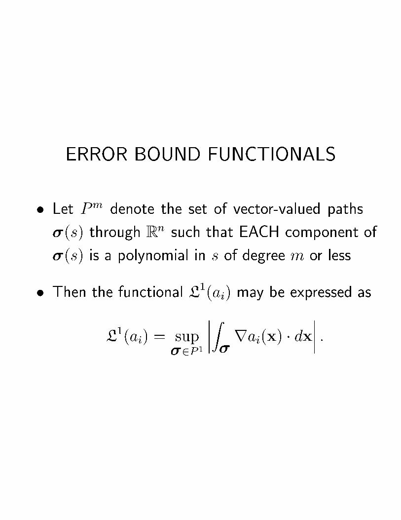
ERROR BOUND FUNCTIONALS
� Let Pmdenote the set of vector-valued paths
�(s) through Rnsuch that EACH component of
�(s) is a polynomial in s of degree m or less.
� Then the functional L1(ai) may be expressed as
L1(ai) = sup
�2P 1
����Z�rai(x) � dx
���� :

ERROR BOUND FUNCTIONALS: : :
� Let 'i;xk(x) =@
@xk'i(x).
� Then
S1k('i) = sup
�2P 1
Z�jr'i;xk(x)j ds:
� In the n-dimensional discrete `q-space, jjgpjj`q is
the usual norm of gp with respect to the counting
measure:
jjgpjj`q =
8<: Xm2Zn
jgp(m)jq
9=;1
q
:
� When q = 1, jjgpjj`q is the absolute sum of
gp(m).
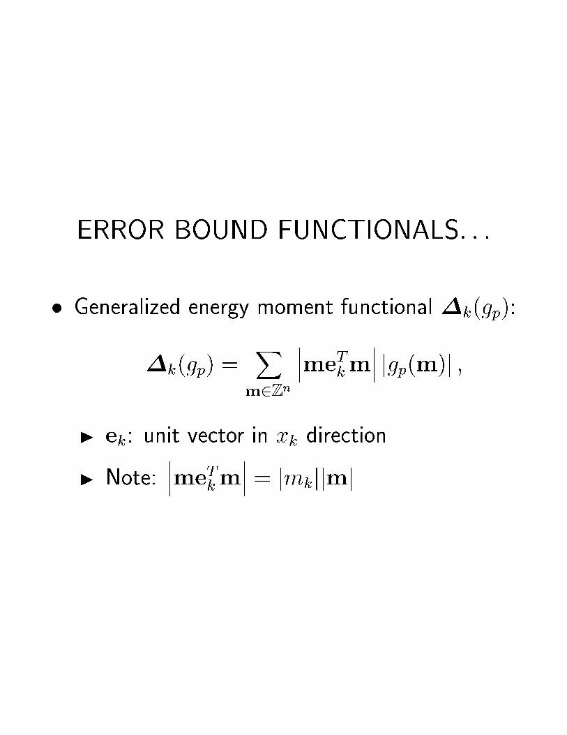
ERROR BOUND FUNCTIONALS: : :
� Generalized energy moment functional �k(gp):
�k(gp) =Xm2Zn
���meTkm��� jgp(m)j ;
I ek: unit vector in xk direction.
I Note:
���meTkm��� = jmkjjmj.

UNFILTERED DEMODULATION
� Amplitude: ai(m) = jti(m)j.
� Let e1 be a horizontal unit vector and e2 be a
vertical unit vector.
� Let k = 1 or k = 2.
� Then, eTkr'i(m) is one component of r'i(m).
� Let hk(m) = �(m+ n1ek) + q�(m+ n2ek).
� Let n1 = 1 and n2 = q = �1. Apply QEA:
eTkr b'i(m) = arcsin
"ti(m+ ek)� ti(m� ek)
2jti(m)
#
� Let n1 = q = 1 and n2 = �1. Apply QEA:
eTkr b'i(m) = arccos
"ti(m+ ek) + ti(m� ek)
2ti(m)
#
� Together, these algorithms place the estimated
frequencies to within 2� radians.

STATE-SPACE MODEL
� Let � denote continuous arc length along P.
� Restrict the derivatives of the modulating func-
tions of ti(�) to the 1D lattice:
a0i(k) =@
@kai(k) =
@
@�ai(�)
������=k
� Expand the modulating functions in �rst-order
Taylor series, e.g.
ai(k + 1) = ai(k) + a0i(k)
+
Z k+1
k(k + 1� �)a00i (�)d�:
� Expand the derivatives of the modulating func-
tions in zeroth-order Taylor series, e.g.
a0i(k + 1) = a0i(k) +
Z k+1
ka00i (�)d�:

STATE-SPACE MODEL: : :
� Consider ai(x) and 'i(x) to be homogeneous,
m.s. di�erentiable random �elds; let 'i(x) be
quadrant symmetric.
� Model the six Taylor series integrals with six
noise processes | ua(k), u'x(k), u'y(k); �a(k),
�'x(k), �'y(k) | called Modulation Acceler-
ations or MA's (local averages of modulating
function second derivatives).
� Model errors in �ltered demodulation algorithm
with uncorrelated Measurement Noises (MN's)
na(k), n'x(k), and n'y(k).

STATE-SPACE MODEL: : :
� Rearrange the six Taylor series and write together
to obtain the statistical state-space component
model266666664
ai(k + 1)
a0
i(k + 1)
'xi(k + 1)
'x0
i(k + 1)
'y
i(k + 1)
'y0
i(k + 1)
377777775=
266666664
1 1 0 0 0 0
0 1 0 0 0 0
0 0 1 1 0 0
0 0 0 1 0 0
0 0 0 0 1 1
0 0 0 0 0 1
377777775
266666664
ai(k)
a0
i(k)
'xi(k)
'x0
i(k)
'y
i(k)
'y0
i(k)
377777775+
266666664
ua(k)
�a(k)
u'x(k)
�'x(k)
u'y (k)
�'y (k)
377777775
Y(k) =
264 ai(k)
'xi(k)
'y
i(k)
375� Observation equation:264 ba(k)c'x(k)c'y(k)
375 =
264 ai(k)
'xi(k)
'y
i(k)
375+
264 na(k)
n'x (k)
n'y (k)
375

PATH FUNCTION
� The TRACK PROCESSOR processes image pixels
in the order speci�ed by P: