Wireless Communication Project (EE381K-11)Technical Report

Optimal Channel Estimation for Capacity Maximizationin OFDM Systems

OFDM-2 GroupWei Wu, Vikrant V. Gunna Srinivasan, Chien-fang Hsu, Youngok Kim, Chulhan Lee

Course Instructor: Prof. Theodore RappaportDepartment of Electrical and Computer Engineering

The University of Texas at Austin, Austin, TXE-mail:wwu, sgunna, chsu, ykim4, chlee@ece.utexas.edu

Phone: 512-425-1305

May 6, 2003

Abstract

The capacity of OFDM systems can be achieved by channel estimation and adaptive trans-mission at each subcarrier. Therefore channel estimation techniques play a key role in thedesign of OFDM systems. In this paper, we propose a method to analyze and evaluate the per-formance of various channel estimation techniques. Using the developed optimization model,we can tune various parameters of channel estimation to maximize the capacity of the OFDMsystem taking into consideration the estimation errors and channel uncertainty. This work isdifferent from other works because it doesn’t assume perfect channel information and dealswith estimation errors. We simulate the theoretical model and test the optimal allocation inindoor wireless environment settings.

1

1 Introduction

Orthogonal frequency division multiplexing (OFDM) is a potential technique for transmitting highbit rate data over indoor and outdoor wireless communication systems, which can be seen fromthe facts that it has been widely accepted by most of standards for next generation communicationsystems, such as digital TV, wireless LAN (such as 802.11a and g, HIPERLAN2) and fixed pointwireless communication (802.16). This is due to its simple implementation with high bandwidthefficiency and its robustness to multi-path delay.

The performance of the OFDM system can be vastly increased with dynamic estimation of channelbefore the demodulation of OFDM signals since the wireless channel is frequency selective andtime-varying for wideband mobile communication systems [1]. Furthermore, as shown in [2], withperfect channel information at both the transmitter and receiver, water-filling power allocation andadaptive rate control can achieve higher capacity in a single carrier communication. Then byknowing the channel gain of each sub-carrier, the adaptive transmission can be performed at eachsubcarrier to achieve the maximum data rate allowable. So the channel estimation method playsa critical role in the performance of OFDM systems. Our project studies the optimal design ofchannel estimation to achieve the maximum data throughput under various channel models bytheoretical analysis and simulation.

There are generally two channel estimation techniques used for OFDM channel estimation: fre-quency domain pilot interpolation (FDPI) [3] [5] and time domain training sequence (TDTS) [4].In this work, we focus on the FDPI method, which chooses some subcarriers as pilot tones andmeasures the channel gains of each pilot periodically. The channel gain of the other subcarrierscan be obtained by interpolation. One extreme case, the block type pilot arrangement inserts pilottones into all of the subcarriers of OFDM symbols with a specific period; and another extremecase, the comb type pilot arrangement inserts certain number of pilot tones into each OFDM sym-bol. There are lots of other pilot patterns between the two extreme cases. How to place the pilottones and in what period to achieve the maximum system capacity is very critical for the design ofOFDM systems. From intuition, the more pilot tones we use, the more accurately we estimate thechannel thus increasing the achievable capacity. On the other hand, the more resource we use forpilot tones, the more overhead of the system. So there is a tradeoff between the pilot arrangementand the system capacity and the optimal arrangement exists in term of system capacity.

In this technical report, we develop the analytical models and simulation tools to optimize the pilotarrangement patterns to achieve the maximum capacity. The method and part of the results can beapplied to lots of communication systems with imperfect channel information.

2

2 System Description

Figure 1 shows the OFDM system we consider in our work. At the transmitter, input binarydata are first mapped to some symbols by modulation (QPSK, QAM, etc), and these symbolsare modulated ontoN orthogonal subcarriers. Since each of these streams are assumed to bein the frequency domain, IDFT is used to convert the frequency domain signals to time domainsignals. Then a guard interval is inserted in front of the transmitted symbol to eliminate inter-symbol interference(ISI). Besides, to estimate the channel gains in the frequency domain, severalsubcarriers are selected as pilot tones which transmit pre-known data to the receiver. Then thetransmitted symbols are passed through the channel model, which will be described in the nextsection.

Figure 1: OFDM system block diagram with Optimizer.

At the receiver, the demodulation follows the reverse procedures performed at the transmitter:the guard interval is removed from the received symbols, and the symbol is then transformedfrom the time domain to the frequency domain by Discrete Fourier Transform (DFT). Since thedata transmitted in the pilot tones are pre-known at the receiver, it can obtain the channel gainsby channel estimation. Then the optimizer can get the channel gains of all other subcarriers byinterpolation, and then optimize the power allocation and the pilot tone placement.

3

3 Channel Model

In wireless communication system simulation, the channel model plays a very important role sincein different wireless environments, channel characteristics may be totally different. To compare theperformance of different pilot placement, we will use three channel models in different wirelessenvironments to test the proposed algorithms. They are models of the indoor environment ofwireless LAN, Stanford University Interim channel models of wireless MAN and WAN, and thechannel model for the 3rd generation cellular systems.

3.1 Indoor Channel model

The indoor wireless channel model is one of the key topics in the area of channel propagationsince the radio signals in the indoor environment are distorted seriously by the highly reflectiveand shadowing effects. Since 1980s, various measurements and models of indoor environmentsare published in the literature. Even though the Doppler shift is very small due to the low mobilityof users in the indoor environment, the indoor channel is still a hostile environment for wirelesscommunications because of serious multipath fading.

In this project, a channel model [7] recommended as a criterion by IEEE for performance evalu-ation of WLAN systems is used for simulation. As Figure 2 shows, the impulse response of thechannel is composed of complex samples with random uniform phase and Rayleigh distributedmagnitude with exponential decay. Typical root mean square (RMS) delay spread in an indoorwireless environment is showed in Appendix 1.

3.2 Stanford University Interim Channel Model

Stanford University Interim(SUI) channel models are proposed in[8] to simulate, design, develop,and test a system suitable for fixed broadband wireless applications. There are total 6 types ofSUI channels with different parameters selected for typical terrain types of the continental US.Because SUI is used to model the outdoor environment, the Doppler shift is higher than the indoorenvironment, but it is still low. Tables 2, 3, 4 in Appendix 1 show some important characteristicsof 6 SUI channels [9, 10].

3.3 3G channel Model

The channel models of the 3rd generation mobile communication systems are defined in severalwireless environments, including indoor, indoor plus outdoor, pedestrian, and vehicular. The most

4

8Ts7Ts6Ts5Ts4Ts3Ts2TsTs0

Magnitude

Time

Figure 2: Channel impulse response; black illustrates the average magnitude, gray illustrates themagnitude of a specific random realization; for clarity, time positions of black and gray samplesare offset.

5

challenging one is the vehicular model since the Doppler shift may be up to 200 Hz. Channel delayand power gain in non-static wireless environments are showed in Appendix 1.

3.4 Rayleigh Fading Approximation

Since there are several different kinds of channels in the simulation, it is necessary to use a moreflexible method to model the Rayleigh fading effect. Besides, as the sampling frequency of acommunication system increases, the computation load of Rayleigh fading channel increases dra-matically. Therefore, Jake’s model [12] is used to approximate the Rayleigh distribution. Thefundamental idea of the Jake’s model is to use several sinusoids to model the ring scattering effect,and to place more sinusoids near the maximum Doppler shift. Jake’s model is a function of timewith only one random parameter, the phase of a single sinusoid. Thus, given a maximum Dopplershift, it is easy to calculate the corresponding Rayleigh fading response for any time period preci-sion. For more details, please refer to Appendix 2.

4 Channel Estimation

Since the channel gain is a factor in the optimization function for maximum capacity, more accu-rate channel gain estimation is required in the receiver. A pilot tone is the selected subcarrier totransmit the training data. With pilot tones, the characteristics of channel are estimated by com-paring the transmitted data and received data at the receiver, because the pre-known training datais transmitted to the receiver.

(a) (b)

Figure 3: Two typical types of pilot arrangement; (a) Block type; (b) Comb type;

6

Figure 3 shows two types of channel estimation methods, comb and block type. Both of them areconsidered for channel estimation for pilot tones. The comb type channel estimation assignsLsubcarriers as pilot tones in theN subcarriers, (L < N ), in each symbol, while the block typeuses all subcarriers as pilot tones in a selected symbol during transceiving. WhenM symbols aretransmitted, if the number of pilot tones is the same in two types, we can combine both types inour channel estimation method to achieve optimal pilot pattern amongM symbols. The Mini-mum Mean Square Error (MMSE) expression is used for the channel estimation of the first orderMarkov channel model(Appendix 3) in the following section. The following mathematical analysisis reproduced from [3].

When a symbol consists ofN data packets modulated ontoN subcarriers and the noise is AWGN(Vk,m, wherek represents the index of pilot tone andm represents the index of symbol), the systemcan be expressed in the frequency domain as

Yk,m = Hk,mXk,m + Vk,m, k = 0, 1, ..., N − 1; (1)

Rk,m = Hk,m +Sk,m

|Xk,m| , k = 0, 1, ..., N − 1, (2)

whereXk,m andYk,m represent the transmitted and received data respectively;Hk,m is channel gain;Sk,m =

Vk,m

ej 6 Xk,m

; Rk,m =Hk,m

Xk,m.

WhenXk,m are pre-known data (pilot tones),Rk,m is the estimated channel gain on thekth sub-carrier. Then the collection ofRk,m makes vectorRm. For example, ifN = 6 and the indices ofpilot tones are 1, 3, and 5, then[ R1,m R3,m R5,m ] = Rm. From Equation 2, we can make vectorequation about pilot tones as

Rm = Hm +Sm

|Xm| . (3)

The estimate is derived by IFFT ofRm and is expressed as

rm = IFFT (Rm)

= hm + IFFT (1√εx

Sm)

= hm +1√εx

Q−1Sm, (4)

where√

εx is a constant modulus of training data andQ is matrix expression of IFFT.

In Equation 4, since the{S1,m, S2,m, S3,m, ...SL,m} are i.i.d. random variables with the variance,the Mean Square Error (MSE) in the channel estimate can be driven as

7

MSE = E{‖rm − hm‖2}

=σ2

s

εx

tr{(Q∗Q)−1}, (5)

whereQ∗ is the complex conjugate ofQ, andtr{(Q∗Q)−1} = L2/N . Therefore, without aprioriknowledge of the channel gains, the channel can be estimated by minimizing Eqaution 5.

For OFDM symbolm, the algorithm of the channel estimation follows as

rm = IFFT (Rm);

hm = hm−p + (1− β)rm, (6)

whereβ is the forgetting factor andp is the time interval between pilot tones(for example, in combtype,p = 1).

When the channel estimation is the in the steady state, the optimal forgetting factor,βopt, can becomputed to minimize theMSE in Equation 5, The Minimum Mean Square Error (MMSE) isexpressed as

MMSE =Nσ2

s

εx

(β2

opt

1− β2opt

ηs +1− β2

opt

1 + β2opt

), (7)

whereβopt = 1 + ηs

2−

√ηs + η2

s

4andηs = tr{Rw}εx

Nσ2s

. As for theηs, it is an indicator of the rate ofchannel variation (Appendix 3).

Finally, the channel estimation method for the pilot tones is

h0 = 0;

rm = IFFT (Rm);

hm = hm−p + (1− β)rm;

Hm = FFT (hm),

wherem is the index of the symbol.

5 Weighted Water filling: optimal rate achievable under chan-nel uncertainty

In this section, we formulate a capacity maximization problem in OFDM system to optimize itscapacity by optimal channel estimation and power allocation. As we have shown, the channel

8

condition can be measured at some time instance by sending pilot tones and utilizing estimators,such as MMSE. In the first part of this section, we will develop the optimal linear interpolation toestimate the channel gains at subcarriers other than selected pilot tones. Moreover, by exploitingthe channel time correlation, we can predict the channel gains and its variance. In the second partof this section, a weighted water-filling is proposed to optimize the OFDM system capacity underuncertain channel information.

5.1 Channel interpolation and prediction

In the previous section, we have described the method to estimate the channel gains at the selectedpilot tones. Once we know the gains of pilot tones at one a instance, we need to extend theestimation to other subcarriers by exploiting the channel correlations at both frequency and timedomain. In this subsection we will develop the method for channel estimation interpolation in thefrequency domain and prediction in the time domain.

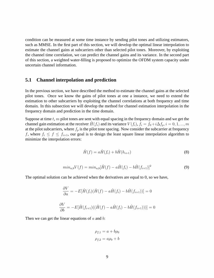
Suppose at timet, m pilot tones are sent with equal spacing in the frequency domain and we get thechannel gain estimation at the receiverH(fi) and its varianceV (fi), fi = f0+i∆fp, i = 0, 1, ..., mat the pilot subcarriers, wherefp is the pilot tone spacing. Now consider the subcarrier at frequencyf , wherefi ≤ f ≤ fi+1, our goal is to design the least square linear interpolation algorithm tominimize the interpolation errors:

H(f) = aH(fi) + bH(hi+1) (8)

mina,bV (f) = mina,b[H(f)− aH(fi)− bH(fi+1)]2 (9)

The optimal solution can be achieved when the derivatives are equal to 0, so we have,

∂V

∂a= −E[H(fi)(H(f)− aH(fi)− bH(fi+1))] = 0

∂V

∂b= −E[H(fi+1)((H(f)− aH(fi)− bH(fi+1)))] = 0

Then we can get the linear equations ofa andb:

ρf,1 = a + bρ0

ρf,2 = aρ0 + b

9

whereρ1, ρ2 are the correlation coefficient betweenH(f) andH(fi),H(fi+1) respectively, whilerho0 is the correlation coefficient between two adjacent pilot subcarriers. According to the deriva-tion in chapter 4 of [18], the correlation coefficients of two channel gains with the frequencydifference∆f and the time differenceτ can be demonstrated by

ρr =J2

0 (2πfmτ)

1 + (2πδfT )2(10)

where T is the mean time delay of the multipath channel,fm is the maximum Doppler fre-quency shift andJ0(·) is the first order Bessel function. Then we can findρ0 = 1

1+(2πfp)2,

ρf,1 = 11+[2π(f−fi)]2

, ρf,2 = 11+[2π(fi+1−f)]2

. Solving the linear equation, we can know the parametersof the optimal interpolation:

a =ρf,1 − ρf,2

1− ρ20

(11)

b =ρf,2 − ρf,1

1− ρ20

(12)

Moreover, the interpolation errors can be obtained oncea, b are known:

V (f) = (1− a2 − b2)σ2 (13)

whereσ2 is the variance of the channel gain.

Next we obtain the channel prediction by Gauss-Markov model described in the last section:

H(f, t + 1) = ρtH(f, t)

V (f, t + 1) = V (f, t) + (1− ρ2t )σ

2

whereρt is the correlation coefficient between two OFDM symbol time instants. According to(10),ρt = J2

0 (2πfmTs), whereTs is the duration of an OFDM symbol.

5.2 Capacity Maximization under channel information uncertainty

As shown in the other works [20], the capacity of OFDM systems can be achieved with perfectchannel information by water-filling: pour more power to the subcarriers with better gains. How-ever, the reality is not so optimistic because: (1) the wireless channel is time-varying and only

10

previous channel information is available; (2) the channel estimation techniques are not perfectand there are always some estimation errors; (3) some other sources (e.g., inter-carrier interfer-ence, mis-synchronization) can introduce errors to the channel estimation.

As derived in the previous section, the channel gains and their variance can be calculated based onthe measurement of pilot tones. Then the question is ”how to accommodate the channel uncertaintyfor power allocation?” and furthermore, ”how to place the pilot tones in the time and frequencydomain to maximize the system efficiency in some performance metric”.

In this paper, we use the outage capacityCoutage as our performance metric, soCoutage = E[1(r <CShannon)CShannon], wherer is the transmission rate andCShannon is the ergodic capacity devel-oped by Shannon. The explanation of the definition is straightforward: when the transmission rateis higher than the Shannon capacity, the transmission will not be successful because of the unre-coverable errors. In the wireless system with adaptive transmission, the channel information ismeasured at the receiver and feedback to the transmitter; the transmitter chooses the transmissionpower and rate adaptively to exploit the highest possible throughput. So in the practical wirelesssystem subject to various errors, when the channel gains are over-estimated, higher than its realvalue, a transmission rate higher than the Shannon capacity might be selected thus making unre-coverable errors and transmission failure. But if we overly underestimate the channel gain, theselected data rate based on the estimation might be much less than the maximum allowable datarate, which results in the inefficiency of resource usage. So our objective is to maximize the sumcapacity of data throughputC,

maxPi,HC = maxPi,H

N∑i=1

Pr(H(f) > H)fslog2(1 +PiH

N0fs

) (14)

subject to the total power constraints:

N∑i=1

Pi ≤ Pmax

Pi ≥ 0

Hi ≥ 0

Where N is the number of subcarriers,H is the channel estimate, which is a Gaussian distributedrandom variable with meanH and varianceV . To solve the optimization problem with a constraint,we can define the Lagrangian and apply the first order necessary condition [19]:

11

L(P, H, λ) =N∑

i=1

Pr(H(f) > H)fslog2(1 +PiH

N0fs

) + λ(N∑

i=1

Pi − Pmax)

∂L(P, H, λ)

∂Pi

=Pr(Hi > Hi)

ln2·

Hi

N0fs

1 + PiHi

N0fs

+ λ = 0 (15)

∂L(P, H, λ)

∂Hi

= −log2(1 +PiHi

N0fs

) · fG(Hi) +Pr(Hi > Hi)

ln2·

Pi

N0fs

1 + PiHi

N0fs

= 0 (16)

wherefG(x) = 1√2πσx

exp(− (x−Ex)2

2σ2x

) is Gaussian distribution probability density function and

Pr(Hi > Hi) =∫ +∞

HifG(Hi)dHi is the Gaussian cumulative distribution function. The optimal

solution can be obtained by applying the method introduced in [19] (e.g., Newton-Rapson method).One thing needed to remind is that the objective function (14) is not concave in the constrainedregion so that the global optimizer cannot be guaranteed to be achieved by those algorithms andonly the local optimizer can be obtained.

By carefully formulating Equ.15, we can obtain the following equation:

Pi = max(Pr(Hi > Hi)

λln2− N0fs

Hi

, 0) (17)

Comparing Equ.17 with conventional water-filling [20] under perfect channel information, thedifference is the factorPr(Hi > Hi), so we call it weighted water-filling algorithm. The weightsare decided by the variance of channel estimation. So the optimal capacity of the system is notonly decided by channel gains, but also in what extent the channel uncertainty is. To demonstratethe weighted water filling more clearly, we draw the power allocation in Figure.4 in the case thatall subcarriers have the same channel gain estimationHi but different varianceVi, Vi = 0.01 × i.We can see the weighted water filling algorithm is prone to allocate more power to the channelwith less channel uncertainty.

6 Simulation Results

In the simulation phase of the project, the OFDM system was simulated in Matlab in a slow andfrequency selective fading indoor channel. Uncoded 4-QAM modulation was assumed. Initiallythe OFDM system was simulated without channel estimation. Next channel estimation was intro-duced through pilot tones.During each run of the simulation, the following parameters were fixed:

12

1 2 3 4 5 6 7 8 9 100

0.02

0.04

0.06

0.08

0.1

0.12

0.14

User #

Pow

er o

f use

i

The effect of estimation errors on Power allocation

Figure 4: Weighted water filling even when the channel gains are all equal for all 10 subcarriers.

the number of OFDM symbols, the number of sub carriers in each symbol. Figure 5 represents atime frequency slot that is transmitted.

From Figure.5 we note that there areN subcarriers andM symbols in a slot. To simulate anindoor environment a Rayleigh channel model is simulated using the Jakes Model with a Dopplerfrequency of1 Hz. Initially the power that is transmitted is equally distributed across all thesubcarriers in the symbol. At the receiver, the channel gain is calculated at pilot tones through theMMSE algorithm. The channel optimizer interpolates the gains at the pilot tones to obtain the gainat each subcarrier. The output of this module is the power allocation at each subcarrier.

We present two sets of results, one for an OFDM system wherein the number of pilot tones werefixed and the pilot period i.e. the periodicity with which the pilot tones are inserted into the OFDMframes, was varied and the other, wherein the pilot period was fixed and the number of pilot toneswere increased. So depending on the simulation environment the pilot arrangement can either beblock or a comb arrangement.

The first set of results were simulated with 60 symbols, 16 subcarriers in each frame,with 6 pilottones. Figure.6 shows the output capacity.

We note that the capacity drops as the pilot period increases. The optimal allocation occurs whenthe capacity is at its peak, corresponding to a pilot period of 15 symbols.

13

1 2 3 N

1 Pilot tone 1

Pilot tone 2 …

Pilot tone P

…

…

…

…

Pilot tone 1

Pilot tone 2 … Pilot

tone P

…

…

…

…

M Pilot tone 1

Pilot tone 2 … Pilot

tone P

Time Frequency Slot

Subcarrier Index

Sym

bol i

ndex

Figure 5: Time Frequency slot

0 10 20 30 40 50 60200

220

240

260

280

300

320

340

360

380

400

Figure 6: C vs. Pilot Period, 16 Subcarriers

14

Figure 7 was generated by increasing the subcarriers to 40. We note that the optimal period is 5symbols. i.e. the number of pilot tones required has increased. In the third simulation, the number

0 10 20 30 40 50 6020

40

60

80

100

120

140

160

pilot period

C

Capacity vs. Pilot Period

Figure 7: C vs. Pilot Period, 40 Subcarriers

of symbols transmitted was 60 but the number of subcarriers was increased to 64. We note that

0 10 20 30 40 50 60400

450

500

550

600

650

700

C

Pilot Period

Figure 8: C vs. Pilot Period, 64 Subcarriers

according to Figure.8 the peak occurs at approximately pilot period of 3 symbols. Therefore, asthe number of subcarriers increases, the pilot period decreases, which means that the number ofpilot tones required increases.

In the second set of results, the pilot period is fixed and the number of pilot tones is increased. Thenumber of frames is fixed at 4 and the pilot period is set at 3. So the first and the last frame have

15

the pilot tones. Initially the number of subcarriers is fixed at 32. We obtain the graph shown inFigure.9 .

0 20 40 60 80 100 120 14080

100

120

140

160

180

200

220

240Capacity vs. # Pilot tones

# pilot tones

C

Figure 9: C vs. Pilot Tones 32 Subcarriers

We note that the optimal value of pilot tones is 8. Next the number is increased to 64 and from thefigure.10 we note that the optimal number has increased to 16.

0 5 10 15 20 25 30 3580

100

120

140

160

180

200Capacity vs. # Pilot tones

# pilot tones

C

Figure 10: C vs. Pilot Tones 64 Subcarriers

From the results shown, we note that as the number of subcarriers increase, the pilot period de-crease for optimal channel estimation. Also when the pilot period is fixed and the subcarriersincrease, the number of pilot tones required also increase.

16

7 Conclusions and Future works

In this technical report, we have developed both a theoretical method and a simulation tool to studythe relationship between system capacity and channel estimation. We develop a general model tostudy the optimal power allocation with imperfect channel information, and then use it to quantitythe performance of different pilot tone placement. A OFDM simulation tool is also developed inMatlab to simulate various blocks, such as modulation, pilot tone insersion multiplexing, wirelesschannel model, etc.

So the contribution of this project are:

1. Implementation of MMSE channel estimation algorithm;

2. Propose Optimal linear interpolation algorithm

3. Propose a weighted water-filling algorithm to maximize Capacity for wireless systems withchannel uncertainty;

4. Implementation of the whole OFDM system simulation blocks;

5. Development of various wireless channel models in a computation-efficient way in matlabby Jakes model.

In the future work, we will study another channel estimation method: time domain training se-quence method and compare the two method both theoretically and through the simulation. Fur-thermore some information theoretic approach can be proposed to study the maximum mutualinformation under imperfect channel estimation and different channel learning method.

APPENDIX

1 Tables of Channel Parameters

Table 2 categorizes the path loss model. The maximum path loss category is hilly terrain withmoderate-to-heavy tree densities(Category A). The minimum path category is mostly flat terrainwith light tree densities(Category C). Intermediate path loss condidton is captured in Category B.

17

Table 1: Measured delay spread in frequency range of 4 to 6 GHz[6].

Maximumdelay spread (ns) Environment125 Factory120 Stock Exchange120 Indoor sports arena60-65 Office building55 Meeting room with metal walls35 Single room with stone walls

Table 2: Terrain Types of SUI Channels.

Terrain Type SUI ChannelsA SUI-5, SUI-6B SUI-3, SUI-4C SUI-1, SUI-2

Table 3: Doppler and delay spread SUI channels(Low K-factor).

Doppler Low delay spread Moderate delay spreadHigh delay spreadLow SUI-3 SUI-5High SUI-4 SUI-6

Table 4: Doppler and delay spread SUI channels(High K-factor).

Doppler Low delay spread Moderate delay spreadHigh delay spreadLow SUI-1, 2High

18

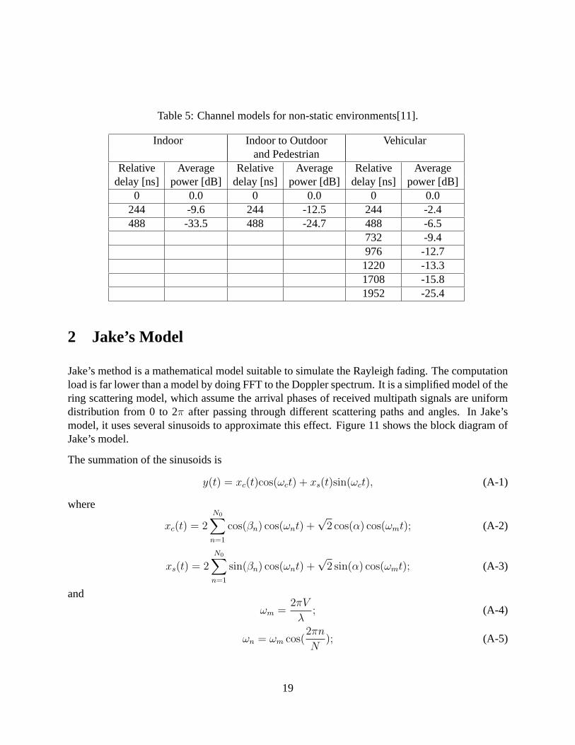
Table 5: Channel models for non-static environments[11].

Indoor Indoor to Outdoor Vehicularand Pedestrian

Relative Average Relative Average Relative Averagedelay [ns] power [dB] delay [ns] power [dB] delay [ns] power [dB]

0 0.0 0 0.0 0 0.0244 -9.6 244 -12.5 244 -2.4488 -33.5 488 -24.7 488 -6.5

732 -9.4976 -12.71220 -13.31708 -15.81952 -25.4

2 Jake’s Model

Jake’s method is a mathematical model suitable to simulate the Rayleigh fading. The computationload is far lower than a model by doing FFT to the Doppler spectrum. It is a simplified model of thering scattering model, which assume the arrival phases of received multipath signals are uniformdistribution from 0 to 2π after passing through different scattering paths and angles. In Jake’smodel, it uses several sinusoids to approximate this effect. Figure 11 shows the block diagram ofJake’s model.

The summation of the sinusoids is

y(t) = xc(t)cos(ωct) + xs(t)sin(ωct), (A-1)

where

xc(t) = 2

N0∑n=1

cos(βn) cos(ωnt) +√

2 cos(α) cos(ωmt); (A-2)

xs(t) = 2

N0∑n=1

sin(βn) cos(ωnt) +√

2 sin(α) cos(ωmt); (A-3)

and

ωm =2πV

λ; (A-4)

ωn = ωm cos(2πn

N); (A-5)

19

Figure 11: Block diagram of Jake’s model

N0 =1

2(N

2− 1). (A-6)

It can be observed that Jake’s model samples more frequencies near the maximum Doppler shift.WhenN0≤8, xc(t) andxs(t) are approximation of Gaussian random process. Therefore,y(t) canbe used to approximate a Rayleigh distribution.

In the simulation,N is set to be 34 andN0 is equal to 8. Figure 12 shows the amplitude and phasetrajectory responses of the Jake’s model. Figure 13 shows the statistics of the amplitude ofy(t),and it is close to a Rayleigh distribution.

3 First Order Markov Channel

If the channel changes slowly in time, it can be adequately represented by first order Markovchannel[15, 16, 17]. Considering the first order markov channel

hm = βhm−1 + ωm−1, Rω = E{ωmω∗m} (A-7)

wherehm is the channel impulse response at time instancem ande the vector sequenceωm isuncorrelated with itself and Gaussian distributed.

20

0 1 2 3 4 5 6 7 8 9 10

x 104

0

0.5

1

1.5

2

2.5

Samples(duration=1s)

Am

plitu

de

−2.5 −2 −1.5 −1 −0.5 0 0.5 1 1.5 2 2.5−2.5

−2

−1.5

−1

−0.5

0

0.5

1

1.5

2

2.5

Real(Xc)

Imag

inar

y(X

s)(a) (b)

Figure 12: Amplitude and phase trajectory responses of Jake’s model; (a) Amplitude response; (b)Phase trajectory response;

0 0.5 1 1.5 2 2.5 30

500

1000

1500

2000

2500

3000

3500

4000

4500

5000Histgram of the amplitude of Rayleigh distribution approximation by Jake model

Amplitude

Figure 13: Amplitude statistics of samples from Jake’s model.

21

In the view of the frequency domain, the channel gainHm is derived by applying DFT tohm.Thus, the first order Markov channel in the frequency domain can be expressed as

Hk,m = βHk,m−1 + Nk, (A-8)

wherek is the index of the subcarrier,β is the forgetting factor andNk is a zero mean Gaussianrandom variable. In addition,β can represent the correlation of the channel gain between two timeinstances. SinceNk is uncorrelated with the channel gain and the variance of each subcarrier isconstant, variance ofNk is (1− β2)σ2

Hk.

Considering the channel gain correlation coefficientρ of the subcarrierk between two time in-stancesm andm− 1, from Equation A-8,

Hk,mH∗k,m−1 = βHk,m−1H

∗k,m−1 + NkH

∗k,m−1. (A-9)

Take the ensemble mean on Equation A-8 and A-9.

E[Hk,m] = βE[Hk,m−1] + E[Nk]

= βE[Hk,m−1]. (A-10)

E[Hk,mH∗k,m−1] = βE[|Hk,m−1|2] + E[NkH

∗k,m−1]

= βE[|Hk,m−1|2] (A-11)

By Equation A-10 and A-11, the correlation coefficient can be expressed as

ρ =E[Hk,mH∗

k,m−1]− E[Hk,m]E[Hk,m−1]

σHk,mσHk,m−1

=β{E[|Hk,m−1|2]− E2[Hk,m−1]}

σ2Hk

= β (A-12)

22

References

[1] Theodore S. Rappaport, ”Wireless communications: principles and practice”, 2nd ed, 2002.

[2] A.J. Goldsmith and P.P. Varaiya, ”Capacity of fading channels with channel side informa-tion”, IEEE Trans on Information Theory, vol 43, no.6, Nov. 1997, pp1986-1992.

[3] Rohit Negi and John Coiffi, ”Pilot tone selection for channel estimation in a mobile OFDMsystem”, IEEE Trans. on Consumer Electronics, vol.44, no.3, Aug. 1998.

[4] Che-Shen Yeh, Yinyi Linand Yiyan Wu, ”OFDM system channel estimation using time-domain training sequence for mobile reception of digital terrestrial broadcasting”, IEEETrans. on broadcasting, vol.46, no.3, Sep. 2000.

[5] Sinem Coleri, Mustafa Ergen, Anuj Puri and Ahmad Bahai, ”Channel estimation techniquesbased on pilot arrangement in OFDM systems”, IEEE Trans. on broadcasting, vol.48, no.3,Sep. 2002.

[6] R. van Nee and R. Prasad,”OFDM Wireless Multimedia Communications,”Artech House,Boston, 2000.

[7] IEEE 802.11 Homepage: http://grouper.ieee.org/groups/802/11/.

[8] V. Erceg et. al, ”An Empirically Based Path Loss Model for Wireless Channels in SuburbanEnvironment,”IEEE J. Selected Areas. in Commun.,Vol. SAC-17, No. 7, pp.1205-1211, Jul.1999.

[9] IEEE Document: 802.16.3c-01/29r4.

[10] IEEE Document: C802.16a-02/41.

[11] 3GPP Document: TS 25.101 v1.0.0.

[12] W. C. Jake,”Microwave Mobile Communications,”Section 1.7, 1974.

[13] M. Speth, S. Fechtel, G. Fock, and H. Meyr, ”Optimum Receiver Design for OFDM-BasedBroadband Transmission-Part 2: A Case Study,”IEEE Trans. Commun.,vol 49, no. 4, Apr.2001.

[14] J. Heiskala and J. Terry,”OFDM Wireless LANs: A Theoretical and Practical Guide,”SAMS, 2nd ed., Sep. 2002.

[15] S. S. Haykin,”Adaptive filter theory,” Englewood Cliffs, NJ: Prentice Hall, 3rd ed., 1996.

23

[16] C. C. Tan, N. C. BeaulieuS, ”On First-Order Markov Modeling for the Rayleigh FadingChannel,”IEEE Trans. Commun.,vol 48, no. 12, Dec. 2000.

[17] M. Medard, ”The Effect upon Channel Capacity in Wireless Communications of Perfect andImperfect Knowledge of the Channel”IEEE Trans. Info. Theory,vol 46, no. 3, May 2000.

[18] Michel Daoud Yacoub, ”Foundations of Mobile Radio Engineering”, by CRC Press LLC,1993.

[19] Ross Baldick, ”Optimization of Engineering Systems”, Course Notes available athttp://www.ece.utexas.edu/ baldick/.

[20] T. Cover and J. Thomas, ”Elements of Information Theory”, Wiley, New York, 1991.

24