alternative fuel transportation optimization tool ... · alternative fuel transportation...
TRANSCRIPT

Alternative Fuel Transportation Optimization Tool: Description,
Methodology, and Demonstration Scenarios
Final Report – September 2015
DOT-VNTSC-FAA-15-11
DOT/FAA/AEE/2015-12
Prepared for:
Federal Aviation Administration Office of Environment and Energy Washington, DC

Notice
This document is disseminated under the sponsorship of the Department of Transportation in the interest of information exchange. The United States Government assumes no liability for the contents or use thereof.
The United States Government does not endorse products or manufacturers. Trade or manufacturers’ names appear herein solely because they are considered essential to the objective of this report.
Alternative Fuel Transportation Optimization Tool ii
REPORT DOCUMENTATION PAGE Form Approved OMB No. 0704-0188
Public reporting burden for this collection of information is estimated to average 1 hour per response, including the time for reviewing instructions, searching existing data sources, gathering and maintaining the data needed, and completing and reviewing the collection of information. Send comments regarding this burden estimate or any other aspect of this collection of information, including suggestions for reducing this burden, to Washington Headquarters Services, Directorate for Information Operations and Reports, 1215 Jefferson Davis Highway, Suite 1204, Arlington, VA 22202-4302, and to the Office of Management and Budget, Paperwork Reduction Project (0704-0188), Washington, DC 20503.
1. AGENCY USE ONLY (Leave blank)
2. REPORT DATE September 2015
3. REPORT TYPE AND DATES COVERED Final Report
4. TITLE AND SUBTITLE Alternative Fuel Transportation Optimization Tool: Description, Methodology, and Demonstration Scenarios
5a. FUNDING NUMBERS FA4SCB, FA4SC5, FA5JC7
6. AUTHOR(S) Kristin C. Lewis, Gary M. Baker, Matthew N. Pearlson, Olivia Gillham, Scott Smith, Stephen Costa, Peter Herzig
5b. CONTRACT NUMBER
7. PERFORMING ORGANIZATION NAME(S) AND ADDRESS(ES) U.S. Department of Transportation John A Volpe National Transportation Systems Center 55 Broadway Cambridge, MA 02142-1093
8. PERFORMING ORGANIZATION REPORT NUMBER DOT-VNTSC-FAA-15-11
9. SPONSORING/MONITORING AGENCY NAME(S) AND ADDRESS(ES) US Department of Transportation Federal Aviation Administration Office of Environment and Energy 800 Independence Ave, SW Washington, DC 20591
10. SPONSORING/MONITORING AGENCY REPORT NUMBER DOT/FAA/AEE/2015-12
11. SUPPLEMENTARY NOTES Program Manager: Kristin C. Lewis
12a. DISTRIBUTION/AVAILABILITY STATEMENT This document is available to the public at the National Transportation Library (http://ntl.bts.gov)
12b. DISTRIBUTION CODE
13. ABSTRACT (Maximum 200 words) This report describes an Alternative Fuel Transportation Optimization Tool (AFTOT), developed by the U.S. Department of Transportation (DOT) Volpe National Transportation Systems Center (Volpe) in support of the Federal Aviation Administration (FAA). The purpose of AFTOT is to help FAA better understand the transportation needs and constraints associated with biofuel feedstock collection, processing, and fuel distribution, specifically alternative jet fuel produced from feedstocks. AFTOT uses scenarios describing potentially available feedstock production and existing transportation infrastructure to generate: locations of potentially supportable biorefineries; optimal transportation routes for moving biofuels from the point of feedstock production/pre-processing to refinement and then to fuel aggregation and storage; allocation of feedstock and fuels among biorefineries and destinations based on demand and efficient transport patterns; and transportation costs, CO2 emissions, fuel burn, and vehicle trips and miles traveled as a result of the transportation of feedstock and fuels. This report describes how AFTOT was developed and the functionality of the tool; it also demonstrates the tool’s capability through the analysis of six scenarios.
14. SUBJECT TERMS alternative jet fuels, alternative fuels, biofuels, Federal Aviation Administration, transportation modeling, transportation network
15. NUMBER OF PAGES 94
16. PRICE CODE
17. SECURITY CLASSIFICATION OF REPORT
Unclassified
18. SECURITY CLASSIFICATION OF THIS PAGE
Unclassified
19. SECURITY CLASSIFICATION OF ABSTRACT
Unclassified
20. LIMITATION OF ABSTRACT Unlimited
NSN 7540-01-280-5500 Standard Form 298 (Rev. 2-89) Prescribed by ANSI Std. 239-18
298-102
Alternative Fuel Transportation Optimization Tool iii

Acknowledgments
The team thanks FAA Sponsor Jim Hileman and Project Manager Aniel Jardines (FAA Office of Environment and Energy) for their support and continuous input. The team would also like to acknowledge valuable input and assistance from the following individuals and organizations who kindly provided expertise, data, and/or feedback during the development of AFTOT.
• John Heimlich (A4A) • Ed Coppola (ARA/CGS) • Michael Wang, Hao Cai, Amgad Elgowainy (Argonne National Laboratory) • Steve Csonka (CAAFI) • Nate Brown (FAA) • Bruce DeSoto, Leslie Robbins, Bill Maclaren (DLA-Energy) • Scott Greene, Raquel Hunt (Federal Railroad Administration) • Jake Jacobson, Gary Gresham (Idaho National Laboratory) • Robert Malina, Mark Staples, Parth Trivedi (Massachusetts Institute of Technology (MIT)) • David Shonnard, Suchada Ukaew (Michigan Technological University) • Laurence Eaton, Matthew Langholtz (Oak Ridge National Laboratory) • Tom Richard (Pennsylvania State University) • Amy Nelson Pipeline Hazardous Materials Safety Administration) • Hakan Olcay (SENASA) • Adam Sparger, Marina Denicoff, and colleagues (USDA Agricultural Marketing Service) • Dave Archer, Joon Hee Lee (USDA Agricultural Research Service) • Pete Riley (USDA Farm Services Agency) • Mike Wolcott, Manuel Garcia-Perez, Carlos Alvarez Vasco, Xiao Zhang (Washington State
University)
Alternative Fuel Transportation Optimization Tool iv

Table of Contents List of Abbreviations ...................................................................................................................... x
Executive Summary ........................................................................................................................ 1
1 Introduction ............................................................................................................................. 4
1.1 Overview .......................................................................................................................... 4
1.2 Need for alternative jet fuels ............................................................................................ 5
1.3 Purpose of Report ............................................................................................................. 6
2 Model Structure ...................................................................................................................... 7
3 Analytical Model Framework ............................................................................................... 12
3.1 GIS Data, Tools and Methods ........................................................................................ 14
3.1.1 Intermodal Network ................................................................................................ 14
3.1.2 Origins..................................................................................................................... 16
3.1.3 Destinations............................................................................................................. 17
3.1.4 Identifying biorefinery candidate locations ............................................................ 18
3.1.5 Known Biorefineries ............................................................................................... 19
3.2 XML Defined Parameters .............................................................................................. 20
3.2.1 Assigning Costs to the Network ............................................................................. 20
3.2.2 Assigning Emissions to Movements ....................................................................... 22
3.3 Interface with Alternative Fuel Production Assessment Tool (AFPAT) ....................... 23
3.4 GIS route identification step .......................................................................................... 24
3.5 Optimization tools and methods ..................................................................................... 24
3.5.1 PuLP optimizer – problem definition ..................................................................... 24
3.6 Reporting Outputs .......................................................................................................... 28
3.7 Map Outputs ................................................................................................................... 28
3.8 Testing and Verification of Model Functions ................................................................ 29
3.9 Known Issues and Limitations ....................................................................................... 30
4 Demonstration of Model Capabilities ................................................................................... 32
4.1 Test Scenario 1 – Small geographical area test case ...................................................... 37
4.1.1 Objective ................................................................................................................. 37
Biofuel Transportation Analysis Tool v

4.1.2 Geographical Scope ................................................................................................ 37
4.1.3 Key Input Parameter Values ................................................................................... 37
4.1.4 Run Summary ......................................................................................................... 37
4.1.5 Results/Conclusions ................................................................................................ 38
4.2 Test Scenario 2 – Regional geographical area test (Gulf Coast).................................... 39
4.2.1 Objective ................................................................................................................. 39
4.2.2 Geographical Scope ................................................................................................ 39
4.2.3 Key Parameter Values............................................................................................. 39
4.2.4 Run Summary ......................................................................................................... 39
4.2.5 Results/Conclusions ................................................................................................ 40
4.3 Test Scenario 3 – Broad regional scenario test .............................................................. 41
4.3.1 Objective ................................................................................................................. 41
4.3.2 Geographical Scope ................................................................................................ 42
4.3.3 Key Parameter Values............................................................................................. 42
4.3.4 Run Summary ......................................................................................................... 42
4.3.5 Results/Conclusions ................................................................................................ 42
4.4 Scenario 4 – Oilseed Breakeven Scenario in North Dakota........................................... 49
4.4.1 Objective ................................................................................................................. 49
4.4.2 Geographical Scope ................................................................................................ 49
4.4.3 Key Parameter Values............................................................................................. 50
4.4.4 Run Summary ......................................................................................................... 50
4.4.5 Results/Conclusions ................................................................................................ 50
4.5 Scenario 5 – Historic Production of Wheat Straw ......................................................... 55
4.5.1 Objective ................................................................................................................. 55
4.5.2 Geographical Scope ................................................................................................ 56
4.5.3 Key Parameter Values............................................................................................. 56
4.5.4 Run Summary ......................................................................................................... 56
4.5.5 Results/Conclusions ................................................................................................ 56
4.6 Scenario 6 – Billion Ton Feedstock Production Scenario.............................................. 59
Alternative Fuel Transportation Optimization Tool vi

4.6.1 Objective ................................................................................................................. 59
4.6.2 Geographical Scope ................................................................................................ 60
4.6.3 Key Parameter Values............................................................................................. 60
4.6.4 Run Summary ......................................................................................................... 60
4.6.5 Results/Conclusions ................................................................................................ 60
5 Conclusion ............................................................................................................................ 69
6 Recommendations for Development of Turn-key Biofuel Feedstock and Fuel Transportation Modeling Tool .............................................................................................................................. 70
6.1 Next Steps ...................................................................................................................... 70
6.2 Future Needs - Additional Future Tasks Necessary to Create a Turnkey Model .......... 71
6.3 AFTOT and Transportation Capacity ............................................................................ 72
6.3.1 Symptoms of a Capacity Issue ................................................................................ 72
6.3.2 Challenges in Addressing Capacity ........................................................................ 72
6.3.3 How to Address Capacity ....................................................................................... 73
7 References ............................................................................................................................. 75
Appendix A – AFTOT Airports List and Abbreviations .............................................................. 76
Appendix B – AFTOT Default DFSP List ................................................................................... 79
Appendix C – XML-based Scenario Input File Example ............................................................. 81
Alternative Fuel Transportation Optimization Tool vii

Tables Table 1: Modal cost units and default values in AFTOT. ............................................................. 21 Table 2: Default vehicle capacities for solids and liquids in AFTOT .......................................... 21 Table 3: CO2 per ton-mile combustion emissions intensities for various transportation modes, generated with GREET1_2014 (CO2 only) ................................................................................... 22 Table 4: Assignment of FAF roadway types to MOVES roadway categories for calculation of CO2 emissions from trucks in AFTOT. ........................................................................................ 23 Table 5: PuLP optimizer problem variables and coefficients. ...................................................... 26 Table 6: PuLP Optimizer Constraints ........................................................................................... 27 Table 7: Key input parameters common to all demonstration scenarios described in this report........................................................................................................................................................ 33 Table 8: Summary of selected inputs and results for Test Scenarios 1-3 .................................... 34 Table 9: Summary of selected inputs and results for Scenarios 4-6. ............................................ 45 Table 10: Destinations receiving jet and/or diesel fuel and percent demand fulfilled at airports and DFSPs for Scenario 4. Note that airport codes and names are listed in Appendix A – Airports Abbreviations. ............................................................................................................................... 51 Table 11: Destinations receiving jet and/or diesel fuel and percent demand fulfilled at airports and DFSPs in Scenario 5. Note that airport codes and names are listed in Appendix A – Airports Abbreviations. ............................................................................................................................... 57 Table 12: Destinations receiving jet and/or diesel fuel and percent demand fulfilled at airports and DFSPs for Scenario 6. Note that airport codes and names are listed in Appendix A – Airports Abbreviations. ............................................................................................................................... 62
Figures Figure 1: Schematic diagram of how a scenario is run in AFTOT, showing the four stages of analysis. The optimization takes into account not just transportation costs but also can incorporate preferences (weightings) for particular modes/routes or other factors. ....................... 8 Figure 2: Assumed supply chain structure for AFTOT optimization. .......................................... 10 Figure 3: Storage and time schematic that looks at minimum and maximum flow constraints on transport system with each node encompassing seasonality and storage ..................................... 11 Figure 4: Analytical tool data flow schematic showing the key components/roles of each component of AFTOT................................................................................................................... 13 Figure 5: Example GIS point layer showing origins for a scenario in which county centroids are used as aggregation points for feedstock produced in the county. The user can set a minimum threshold amount of feedstock production below which origins are eliminated. The size of the preprocessor symbol indicates the amount of feedstock available in the county. . ..................... 17
Alternative Fuel Transportation Optimization Tool viii

Figure 6: Generic example of candidate biorefinery location map generated from agricultural scenario, minimum aggregation threshold information along the transportation network, and optimized routes to final destinations. Note this map does not show the pipeline element of the multimodal network. ..................................................................................................................... 19 Figure 7: Example map output from an AFTOT scenario visualizing the scenario results and demonstrating symbology. .......................................................................................................... 29 Figure 8: Feedstock source, processing type, and destinations for demonstration Scenarios 5-7. 33 Figure 9: Map of Test Scenario 1 showing single origin, biorefinery and destination and demonstrating ability of AFTOT to perform a simple, geographically constrained analysis. ...... 38 Figure 10: Map of Test Scenario 2 demonstrating AFTOT ability to perform a mid-size geographic scope analysis, including utilization of pipeline. . .................................................... 41 Figure 11: Map of Test Scenario 3 showing national scale test scenario processing wheat straw into jet fuel and diesel and transporting over a network including all modes. ........................... 44 Figure 13: Modal contribution to Scenario Costs, CO2 Combustion Emissions, Movements (e.g., truckloads, etc.), and vehicle miles traveled (VMT) for Scenarios 4-6. Note that pipeline contribution to total cost is underestimated due to missing base rate values for some routes. ..... 53 Figure 14: Per gallon cost of transport for fuel delivered in Scenarios 4-6. ................................ 54 Figure 14: Map of Scenario 4 showing optimal routing of North Dakota canola production to candidate biorefineries and destinations (arports and DFSPs). ................................................... 55 Figure 15: Map of Scenario 5 showing a national wheat straw scenario based on historical wheat production patterns, advanced fermentation processing, delivery to airports and DFSPs,, and transporting via all modes.. ........................................................................................................... 59 Figure 16: Map of Scenario 6 showing a national analysis of multiple feedstocks as identified in the Billion Ton Study Update by the U.S. DOE, delivery to airports and DFSPs,, and transporting via all modes. Feedstocks included a) switchgrass processed by advanced fermentation, b) sweet sorghum processed by Fischer-Tropsch, and c) hardwood species processed by pyrolysis. ........ 68
Alternative Fuel Transportation Optimization Tool ix

List of Abbreviations
Abbreviation1 Term AFPAT Alternative Fuel Production Assessment Tool AFTOT Alternative Fuel Transportation Optimization Tool ASCENT Aviation Sustainability Center (FAA Center of Excellence) BTAT Biofuel Transportation Analysis Tool (original name of AFTOT) BTS Bureau of Transportation Statistics CAAFI Commercial Aviation Alternative Fuels Initiative CO2 Carbon dioxide COIN-OR Computational Infrastructure for Operations Research project DFSP Defense Fuel Supply Point DOD Department of Defense DOT Department of Transportation EPIC Environmental Policy Integrated Climate (model) FAA Federal Aviation Administration FHWA Federal Highway Administration FRA Federal Railroad Administration GIS Geographic Information System NTAD National Transportation Atlas Database NRCS Natural Resource Conservation Service ONR Office of Naval Research PHMSA Pipeline and Hazardous Materials Safety Administration PuLP Open Source Python Wrapper for Optimization Solvers SSURGO Soil Survey Geographic Database USACE U.S. Army Corps of Engineers USDA U.S. Department of Agriculture VMT Vehicle miles traveled
1 Abbreviations for airports included in the AFTOT destinations layer can be found in Appendix A – Airports Abbreviations.
Alternative Fuel Transportation Optimization Tool x
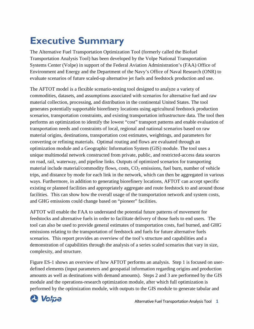
Executive Summary The Alternative Fuel Transportation Optimization Tool (formerly called the Biofuel Transportation Analysis Tool) has been developed by the Volpe National Transportation Systems Center (Volpe) in support of the Federal Aviation Administration’s (FAA) Office of Environment and Energy and the Department of the Navy’s Office of Naval Research (ONR) to evaluate scenarios of future scaled-up alternative jet fuels and feedstock production and use.
The AFTOT model is a flexible scenario-testing tool designed to analyze a variety of commodities, datasets, and assumptions associated with scenarios for alternative fuel and raw material collection, processing, and distribution in the continental United States. The tool generates potentially supportable biorefinery locations using agricultural feedstock production scenarios, transportation constraints, and existing transportation infrastructure data. The tool then performs an optimization to identify the lowest “cost” transport patterns and enable evaluation of transportation needs and constraints of local, regional and national scenarios based on raw material origins, destinations, transportation cost estimates, weightings, and parameters for converting or refining materials. Optimal routing and flows are evaluated through an optimization module and a Geographic Information System (GIS) module. The tool uses a unique multimodal network constructed from private, public, and restricted-access data sources on road, rail, waterway, and pipeline links. Outputs of optimized scenarios for transporting material include material/commodity flows, costs, CO2 emissions, fuel burn, number of vehicle trips, and distance by mode for each link in the network, which can then be aggregated in various ways. Furthermore, in addition to generating biorefinery locations, AFTOT can accept specific existing or planned facilities and appropriately aggregate and route feedstock to and around those facilities. This can show how the overall usage of the transportation network and system costs, and GHG emissions could change based on “pioneer” facilities.
AFTOT will enable the FAA to understand the potential future patterns of movement for feedstocks and alternative fuels in order to facilitate delivery of those fuels to end users. The tool can also be used to provide general estimates of transportation costs, fuel burned, and GHG emissions relating to the transportation of feedstock and fuels for future alternative fuels scenarios. This report provides an overview of the tool’s structure and capabilities and a demonstration of capabilities through the analysis of a series scaled scenarios that vary in size, complexity, and structure.
Figure ES-1 shows an overview of how AFTOT performs an analysis. Step 1 is focused on user-defined elements (input parameters and geospatial information regarding origins and production amounts as well as destinations with demand amounts). Steps 2 and 3 are performed by the GIS module and the operations-research optimization module, after which full optimization is performed by the optimization module, with outputs to the GIS module to generate tabular and
Alternative Fuel Transportation Analysis Tool 1

geospatial reports of the results. Further detail on the elements of each module and the associated analysis components can be found in the main report.
Figure ES- 1: Overall components of AFTOT analysis
The report below gives an overview of the software tool structure, the development of the geospatially-explicit, flowable, multimodal network, the implementation of a supply chain structure that includes multimodal transport routing, pathway specific conversion factors and yields, and a biorefinery siting mechanism based on transportation costs and other constraints, and the use of the tool to analyze six different scenarios. Three of the scenarios described are test scenarios demonstrating capabilities of the tool at multiple scales (from a few counties to the national level) and three national-level scenarios focus on real analyses of interest to FAA. These three scenarios are:
• Movement of oilseeds from North Dakota (based on USDA break-even modeling) and resulting HEFA fuels to end destinations (commercial airports and DOD Defense Fuel Supply Points (DFSPs))
Alternative Fuel Transportation Optimization Tool 2

• Movement of wheat straw based on national wheat production scenarios from historical data (USDA National Agricultural Statistical Survey 2014), converted into jet fuel via advanced fermentation, and delivered to commercial airports and DFSPs
• Movement of multiple feedstocks (switchgrass, sorghum, and hardwoods) based on US Department of Energy’s Billion Ton Study Update, converted via advanced fermentation, Fischer-Tropsch, and pyrolysis, respectively, and the resulting fuel delivered to airports and DFSPs.
The results of these scenarios are presented in the report.
Alternative Fuel Transportation Optimization Tool 3

1 Introduction
1.1 Overview
Alternative fuels are being developed with the hope of mitigating climate change, enhancing energy security, and reducing fuel prices. They are also seen as part of the solution to achieving the aviation sector’s goal of carbon neutral growth in international aviation starting in 2020. Successful scale-up of the incipient alternative jet fuels industry requires appropriate transportation mode choice and pathway selection – and appropriate transportation planning at local, regional, and national scales – to accommodate a shift in energy transportation patterns and accommodate increased production and movement of biofuel feedstocks. The Alternative Fuel Transportation Optimization Tool has been developed by the Volpe National Transportation Systems Center (Volpe) in support of the Federal Aviation Administration’s (FAA) Office of Environment and Energy and the Department of the Navy’s Office of Naval Research (ONR).
The AFTOT model is a flexible scenario-testing tool designed to analyze a variety of commodities, datasets, and assumptions associated with scenarios for fuel and raw material collection, processing, and distribution in the continental United States. The tool generates potentially supportable biorefinery locations using agricultural feedstock production scenarios, transportation constraints, and existing transportation infrastructure data. The tool then performs an optimization to identify the lowest “cost” transport patterns and enable evaluation of transportation needs and constraints of local, regional and national scenarios based on raw material origins, destinations, transportation cost estimates, weightings, and parameters for converting or refining materials. Optimal routing and flows are evaluated through an optimization module and a Geographic Information System (GIS) module. This optimization includes recommended biorefinery locations taken from the candidate list. The goal of the optimization is to minimize the total annual “cost” of maximizing fulfillment of fuel demand utilizing multiple fuel-producing crops and transportation modes. The “cost” in the optimization includes dollar costs of transporting the material over each mode and transloading point, but also weightings and penalties that force the tool to favor particular desirable characteristics of the routing (e.g., prefer interstate highways over smaller roadways). The tool uses a unique multimodal network constructed from private, public, and restricted-access data sources on road, rail, water and pipeline links. Outputs of optimized scenarios for transporting material include material/commodity flows, costs, CO2 emissions, fuel burn, number of vehicle trips, and distance by mode for each link in the network, which can then be aggregated in various ways. Furthermore, in addition to generating biorefinery locations, the system can accept specific existing or planned facilities and appropriately aggregate and route feedstock to and around those
Alternative Fuel Transportation Analysis Tool 4

facilities. This can show how the overall usage of the transportation network and system costs, and GHG emissions could change based on “pioneer” facilities.
This tool builds on the original “Biofuel Transportation Analysis Tool,” or BTAT, that Volpe developed for ONR and FAA (Lewis et al. 2014). The original BTAT focused on analyzing transportation flows via road and rail for oilseed movement, conversion into advanced alternative jet fuels, and downstream flow of jet fuel to Defense Logistics Agency-Energy (DLA-Energy) Defense Fuel Supply Points (DFSPs). AFTOT has been expanded to include waterway (barge) and pipeline modes, to address multiple commodity and processing options, and to incorporate time-steps and storage to enable more detailed analyses based on seasonality of harvest and flows. AFTOT also uses a set of commercial airports and DFSPs as default end destinations, but this can be changed for any scenario given a set of destination points and demand amounts. AFTOT will provide the FAA and other government agencies the ability to test various future alternative fuel transportation scenarios, explore the resulting transportation patterns, needs, and challenges, identify opportunities for alternative fuel production and distribution, and evaluate fuel burn, emissions, and costs associated with these scenarios.
1.2 Need for alternative jet fuels
Dramatic fuel cost increases (Airlines For America 2012), concerns about supply security, and concerns about greenhouse gas (GHG) emissions have led to the FAA’s interest in alternative jet fuels. The FAA has set a target to have one billion gallons of alternative jet fuel in use in 2018 (Federal Aviation Administration 2011). To support this goal FAA has been actively working toward the development and deployment of drop-in alternative jet fuels through its sponsorship of the Commercial Aviation Alternative Fuels Initiative (CAAFI®) and other research programs such as the “Aviation Sustainability CENTer” (ASCENT) Center of Excellence. Together the military and commercial aviation sectors have a significant need for reliable supplies of sustainable alternative aviation fuels that can be distributed throughout the DOD and commercial aviation supply chain domestically and globally. Because little U.S. alternative jet fuel production exists, there is a high level of interest in exploring the production and distribution of a future, scaled-up alternative jet fuel supply. Producing dedicated alternative energy crops, including oilseeds (such as canola, camelina, and pennycress), forage sorghum, sugar cane, lignocellulosic crops (such as perennial grasses), and others, will lead to downstream requirements for transportation to biorefineries and fuel destinations. Furthermore, transportation costs for moving biomass feedstock and resulting fuel substantially influence economic considerations for growing bioenergy crops. The amount of fuel burned in transporting raw feedstocks and finished fuels will influence the overall greenhouse gas (GHG) life cycle emissions of the finished fuel.
Alternative Fuel Transportation Optimization Tool 5

1.3 Purpose of Report
AFTOT will enable the FAA to understand the potential future patterns of movement for feedstocks and alternative fuels in order to facilitate delivery of those fuels to end users. The tool can also be used to provide general estimates of transportation costs, fuel burned, and GHG emissions relating to the transportation of feedstock and fuels for future alternative fuels scenarios. This report provides an overview of the tool’s expanded structure and capabilities and a demonstration of capabilities through the analysis of a series scaled scenarios that vary in size, complexity, and structure.
Alternative Fuel Transportation Optimization Tool 6

2 Model Structure The overall goal of this project was to develop a model to translate a feedstock production/alternative fuel demand scenario into a geospatially explicit result indicating:
• How biorefineries may be sized and spatially distributed • End-to-end route optimization over a national intermodal network • Potential impacts of agricultural scenarios and/or transportation constraints on:
o Material/commodity flows o Transportation costs associated with each movement o Fuel burn and CO2 emissions associated with transport of feedstock and fuel o Total network distance traversed (by mode) o Vehicle miles traveled (VMT) o Number of vehicle trips (e.g., number of truck trips, rail cars, etc.)
The tool incorporates a Geographic Information System (GIS) module and an optimizer module adapted from an open source tool. The structure and function of the modules is described in more detail in the following chapter. These two modules interact to identify candidate biorefinery locations and then allocate flows among the least cost routes between each origin and destination pair, in which cost includes transportation costs per ton-mile for road, rail, and waterway; costs per origin-destination pair in pipeline; transloading costs; and any weightings or preferences incorporated. The schematic approach to this analysis is shown in Figure 1.
Alternative Fuel Transportation Analysis Tool 7

Figure 1: Schematic diagram of how a scenario is run in AFTOT, showing the four stages of analysis. The optimization takes into account not just transportation costs but also can incorporate preferences (weightings) for particular modes/routes or other factors.
Alternative Fuel Transportation Analysis Tool 8
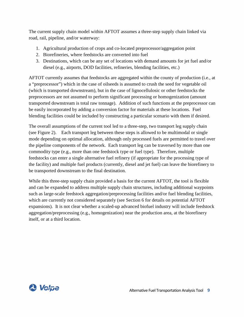
The current supply chain model within AFTOT assumes a three-step supply chain linked via road, rail, pipeline, and/or waterway:
1. Agricultural production of crops and co-located preprocessor/aggregation point 2. Biorefineries, where feedstocks are converted into fuel 3. Destinations, which can be any set of locations with demand amounts for jet fuel and/or
diesel (e.g., airports, DOD facilities, refineries, blending facilities, etc.)
AFTOT currently assumes that feedstocks are aggregated within the county of production (i.e., at a “preprocessor”) which in the case of oilseeds is assumed to crush the seed for vegetable oil (which is transported downstream), but in the case of lignocellulosic or other feedstocks the preprocessors are not assumed to perform significant processing or homogenization (amount transported downstream is total raw tonnage). Addition of such functions at the preprocessor can be easily incorporated by adding a conversion factor for materials at these locations. Fuel blending facilities could be included by constructing a particular scenario with them if desired.
The overall assumptions of the current tool led to a three-step, two transport leg supply chain (see Figure 2). Each transport leg between these steps is allowed to be multimodal or single mode depending on optimal allocation, although only processed fuels are permitted to travel over the pipeline components of the network. Each transport leg can be traversed by more than one commodity type (e.g., more than one feedstock type or fuel type). Therefore, multiple feedstocks can enter a single alternative fuel refinery (if appropriate for the processing type of the facility) and multiple fuel products (currently, diesel and jet fuel) can leave the biorefinery to be transported downstream to the final destination.
While this three-step supply chain provided a basis for the current AFTOT, the tool is flexible and can be expanded to address multiple supply chain structures, including additional waypoints such as large-scale feedstock aggregation/preprocessing facilities and/or fuel blending facilities, which are currently not considered separately (see Section 6 for details on potential AFTOT expansions). It is not clear whether a scaled-up advanced biofuel industry will include feedstock aggregation/preprocessing (e.g., homogenization) near the production area, at the biorefinery itself, or at a third location.
Alternative Fuel Transportation Analysis Tool 9

Figure 2: Assumed supply chain structure for AFTOT optimization.
The original BTAT focused solely on annualized flows. AFTOT analyses can be focused on annual aggregate production, demand, and flows, but can also be used at a more detailed time-specific level to explore seasonal aspects of transportation patterns (e.g., due to seasonality of feedstock harvest and transport). To incorporate seasonality, the tool includes a storage option for each transport path at each time step. Currently, storage is unlimited and has zero cost, but these are variables set within AFTOT and can be modified. Storage is most likely to be suggested if production is highly seasonal, exceeding biorefinery capacity for a limited time period such that it makes sense to store the excess and process it later in the year.
To run a short-term scenario, certain parameters including minimum biorefinery size, biorefinery cost to build, demand, and/or feedstock production may need to be divided by the appropriate factor to scale annual values down to the specific time period of interest (e.g., a two-week period would require division of annual values by 26).
Alternative Fuel Transportation Optimization Tool 10

Figure 3: Storage and time schematic that looks at minimum and maximum flow constraints on transport system with each node encompassing seasonality and storage
Alternative Fuel Transportation Analysis Tool 11

3 Analytical Model Framework The analytical framework of AFTOT was built to accommodate the above concept and supply chain structure using two existing software modeling tools, described in more detail in the sections below:
• ESRI ArcMap Version 10.2.2 or later (Geospatial Information System (GIS)) determines the possible routes between sets of origins and destinations, assigns costs to each leg of each route, identifies the least cost paths for each mode, and identifies candidate biorefinery locations. The GIS module also turns the final optimized transportation links into a final, traversed network and then calculates and reports the results of the scenario runs.
• PuLP Version 1.5.4 (Open Source Python Wrapper for Optimization Solvers) is a linear programming modeler written in Python. In AFTOT, PuLP is used to link the solvers in the Computational Infrastructure for Operations Research project (COIN-OR) to ESRI ArcMap.
• The COIN-OR project contains a number of open source optimization models, including a simplex solver (CLP) and a branch and cut solver (CBC) for mixed integer programming. These tools are used to choose biorefineries from among the candidate locations, and to optimize the assignment of feedstock or fuel to each pathway based on least cost to meet the minimum and maximum biorefinery requirements and the destination jet fuel demand (more details on PuLP are provided in Section 3.5.1).
Figure 4 shows AFTOT model data flow between these two tools.
Alternative Fuel Transportation Analysis Tool 12

Figure 4: Analytical tool data flow schematic showing the key components/roles of each component of AFTOT.
Alternative Fuel Transportation Analysis Tool 13

Alternative Fuel Transportation Optimization Tool 14
14
3.1 GIS Data, Tools and Methods
The GIS component of the tool, built on ESRI’s ArcMap, takes advantage of the geospatial data processing power of this software to build an intermodal network, import origins and ultimate destinations, and generate least cost routes for transportation of alternative fuel feedstock and products. In addition, the GIS module turns agricultural data into preprocessor origin locations and identifies potential biorefinery candidate locations based on volume of material being transported over given distances. The GIS module requires geospatial data for each of the nodes in the supply chain to model the complete transportation flow from origin to destination. The integration of the various components of the supply chain into the GIS module is described below.
3.1.1 Intermodal Network
The foundation of AFTOT is its intermodal network, as the network determines the flow pathways available between each origin and destination in the scenario. The network includes the following elements:
• Roadway network from the Federal Highway Administration’s (FHWA) Freight Analysis Framework (FAF version 3.4 (Federal Highway Administration 2013)
• Railway network developed by the Federal Railroad Administration (FRA). AFTOT uses both Class I and non-Class I rail by default, but the user can subset the network input data when building the network (e.g., Class 1 railroads only).
• Waterway network from the Navigable Waterway Links data developed by the United States Army Corps of Engineers and the US DOT Bureau of Transportation Statistics (BTS) and available in the 2011 National Transportation Atlas Database (Bureau of Transportation Statistics 2011).
• Pipeline origin-destination pairs from a proprietary pipeline dataset provided by Levine Associates.
• Intermodal Terminal Facilities – AFTOT uses an adapted, corrected subset of the Intermodal Terminal Facilities data developed by the BTS and available in the 2011 National Transportation Atlas Database (Bureau of Transportation Statistics 2011). Mode shifts in the AFTOT network can only occur and be modeled at these intermodal terminal facility locations.

Alternative Fuel Transportation Optimization Tool 15
Each of these networks was maintained in its own GIS layer, with interfaces between layers occurring at the intermodal facilities. These layers are used to construct a new intermodal network at the beginning of a scenario run. Thus, the user can also replace layer(s) to create a custom network.
The pipeline network was developed with origin-destination pairs (OD pairs) in a privately acquired dataset from Leonard B. Levine Associates that lists OD pairs, specific product movements, and associated tariffs. Pipeline data repair in the current AFTOT development phase focused on pipeline systems of at least 150 miles in length. Ten full pipeline systems and 20 partial pipeline systems were incorporated into the AFTOT network during this phase of work, with finalization of the full pipeline network anticipated in summer of 2015.
Intermodal facilities are locations where material can be moved through intermodal networks (road, rail, pipeline, and waterway), most commonly referred to as transloading. These transloading points are also locations at which transporters are charged additional per gallon or per ton costs. The BTS National Transportation Atlas Database (NTAD) identifies over 3000 intermodal facilities across the U.S. However, this list has not been updated since 2003, and many of the data points are either in incorrect locations, clustered together, or not relevant to the AFTOT network for various reasons. Therefore, Volpe created a subset of this facility list using specific criteria and visual review of satellite imagery to eliminate excess facility points and correct facility locations. Criteria for elimination included: lack of nearby significant intermodal facility in satellite imagery, proximity to other, more accurate intermodal points, points that did not have complete data and/or points that were not applicable to the AFTOT network (e.g., made at least one linkage among road, rail, waterway, and pipeline). Rail intermodal points were added to the remaining list based on movements of specific, feedstock-relevant commodity types in the Railway Waybill Sample to identify potential railway entry points for agricultural commodities, which are likely to enter the system at smaller facilities than the main intermodal terminals identified by BTS. The commodity-specific origins were incorporated into the GIS layer and duplicates eliminated. The final intermodal facilities layer for AFTOT includes 383 unique intermodal facilities tagged specifically for the different modes that interface at each point. As with the agricultural scenario/origin points, this list can be expanded or modified as needed to run different scenarios in AFTOT.

For routing efficiency, the roadway, rail, and waterway networks were simplified using an “unsplitting” procedure to eliminate nodes between adjacent segments of network that have the same characteristics (e.g., peak period speed (road) or inclusion in Strategic Rail Corridor Network (STRACNET)) and where there is no intersection. This technique does not alter the route options along the network, simply reduces the computational requirements and analysis run times.
Currently, no capacity constraints are included in AFTOT. However, transportation capacity will become more important as the alternative fuel industry expands. The ability to address capacity constraints is recommended as part of future AFTOT expansion, which may also require more detailed networks and other data sources.
3.1.2 Origins
AFTOT is capable of accepting gridded, county-level, or other geospatial data describing feedstock origins and production amounts.
In BTAT, the tool focused on using USDA Agricultural Census Data (USDA 2007) to generate a feedstock production scenario based on use, rotation with, or replacement of existing crops. The tool was designed so that a user could select an existing crop (e.g., wheat) from the Agricultural Census for a given year, provide an assumption regarding allocation of acreage to crop production (e.g., 10% of wheat acreage will be available in a given year for crop rotation). The tool then calculates an estimated yield for each county in which there is production and identifies the county centroid as an origin point for feedstock. This origin point then becomes the “preprocessor” location in the supply chain.
AFTOT can also take in gridded data for feedstock production, and currently assigns an average production value to the county centroid in which the grid cell occurs to identify starting points for the feedstock movement. In each case, AFTOT generates a GIS point layer and the associated data of preprocessor counties and production amounts (see Figure 5). The tool can also take in an existing point layer with production amounts as well, for example if a known set of preprocessors, oilseed crushing facilities, or other origins were used.
Alternative Fuel Transportation Optimization Tool 16

Alternative Fuel Transportation Optimization Tool 17
Figure 5: Example GIS point layer showing origins for a scenario in which county centroids are used as aggregation points for feedstock produced in the county. The user can set a minimum threshold amount of feedstock production below which origins are e liminated. The size of the preprocessor symbol indicates the amount of feedstock available in the county. Note that the pipeline network is included in the multimodal network but is not shown on this graphic because it is based on origin/destination pairs from a private dataset. AFTO T Phase 3 will l ikely incorporate a publicly viewable pipeline dataset.
3.1.3 Destinations
AFTOT is capable of using any set of geospatially defined destinations as the endpoints for the analysis. Due to the project focus on alternative jet fuels in particular, AFTOT includes two default GIS layers of destinations for commercial aviation (airports) and the DOD (Defense Fuel Supply Points, or DFSPs). The airports layer is not exhaustive, but includes 79 airports and their current demand based on approximate (rounded) values provided by Airlines for America (A4A). The current default year is 2014. For the DOD, DLA-Energy shared with the project team the top 52 DFSPs that are the dominant recipients of fuels for the DOD and their annual throughput of jet fuel.

3.1.4 Identifying biorefinery candidate locations
AFTOT is able to generate potential candidate biorefinery locations based on preprocessor and DFSP locations, transport costs, distance constraints, and total agricultural feedstock supply, using the following steps:
1. Identify routes and flow directly from origins to ultimate destinations. 2. Identify candidate biorefinery sites that occur at points on the path from origin to
destination where there is potential for sufficient raw material flow to support a biorefinery (value can be set in the scenario XML configuration file and is usually lower than the actual minimum biorefinery size threshold, as additional feedstock may be available to be reallocated to a biorefinery candidate location during optimization).
3. Consider as a candidate site every node on the transportation network at which further flow increases occur up to the maximum raw material flow distance.
As a secondary screening for biorefinery locations, AFTOT uses an inverse distance weighting (IDW) (ESRI undated) to rank potential biorefinery locations based on the distance from preprocessors and the amount of feedstock available within the user-specified distance limit. The IDW formula is as follows: IDW Score = Total Feedstock Available * (1/(Total Transport Distance2)), which is based on a common structure and exponent value for such weightings (Shepard 1968, ESRI undated).
The user can set limits on the actual travel distance feedstock is permitted to travel to reach a biorefinery – this can be constrained due to, for example, trucking regulations related to moving agricultural products, other regulations, policies or incentives, preference for a particular region, or economic considerations. The user sets the maximum transport distance of feedstock over the transportation network in the scenario input file (described in more detail in Section 3.2). The biorefinery candidate siting algorithm checks for sufficient availability of feedstock for a given candidate location based on that distance limit. IDW ranks highest the candidate biorefinery locations with the most feedstock available at the lowest total transport distance; those candidates with a low amount of feedstock available and/or high total transport distances are ranked lower. This IDW ranking allows the user to drop the least feasible biorefinery candidates from consideration. This secondary screening has the effect of keeping the biorefineries relatively close to the preprocessors and allows AFTOT to choose from a wide number of candidate locations to find the optimal locations for biorefineries, while reducing run times in the final analysis. The percentage of candidates to eliminate from consideration is set by the user in the code and can range from 0%, which would preserve all candidates, to 100%, leaving only any pre-funded locations. The decision of how many candidates to eliminate, if any, is based on run-time, as each biorefinery candidate location adds to the computation time, and efficiency,
Alternative Fuel Transportation Optimization Tool 18

because the greater the number of candidates the greater the likelihood of having redundant candidates located within close proximity of each other.
In the interest of preserving as many candidate locations as possible, the scenarios were run with the bottom 25% of the candidate locations removed from consideration Prefunded facilities are not removed from consideration by the IDW ranking process. The candidate biorefinery sites are incorporated into the GIS network for the scenario.
Figure 6: Generic example of candidate biorefinery location map generated from agricultural scenario, minimum aggregation threshold information along the transportation network, and optimized routes to final destinations. Note this map does not show the pipeline element of the multimodal network.
3.1.5 Known Biorefineries
In the case where a particular biorefinery or set of biorefineries either exist or are planned and the user would like to see how inclusion of the fixed biorefinery locations and demand might alter future development, AFTOT can handle a point layer of such facilities. Location, capacity, and facility name are all that is needed to incorporate fixed biorefinery locations into the model. These fixed biorefineries are flagged within the biorefinery GIS shapefile with the value of 1 in the “prefunded” field. All prefunded biorefineries will have a construction cost of zero. These biorefineries do not have a lower bound on their annual processing because existing production could be adjusted; the lower bound is primarily associated with the decision to invest in building
Alternative Fuel Transportation Optimization Tool 19

a new biorefinery. As with the candidate biorefineries, the GIS module then calculates the optimal pathways to the fixed biorefineries from the preprocessors and from the biorefineries to the DFSPs. The routes to/from all biorefineries, fixed and candidate locations, is then passed to the PuLP optimizer for processing along with the other routes for candidate locations generated by AFTOT (as described in the preceding section).
3.2 XML Defined Parameters
AFTOT uses a “scenario file” input approach using an XML-based document. This document tags each potential data source (as a file source, a function, or a specific set value) for functions within AFTOT.
The user is able to specify a number of scenario parameters in the XML input file, including the transportation costs and weightings that will be allocated across the network, the biomass feedstocks and fuel conversion pathways, minimum production floor for agricultural production to be considered, the maximum feedstock transport distance over the network, the size (minimum and maximum) biorefineries, the feedstock and process designation (to enable capital cost, conversion efficiency and product slate to be pulled from the Alternative Fuels Production Assessment Tool (AFPAT) – see Section 3.3) , and the unmet demand penalty, among other variables. The XML file is validated against an XML schema file. An example XML file is shown in Appendix C. A user can create multiple XML files and run a set of scenarios at one time using a set of command line prompts within a batch file.
3.2.1 Assigning Costs to the Network
AFTOT allows the user to define costs to be assigned to each mode, to transloading, and as penalties for particular paths. The cost parameters are summarized in Table 1.
The GIS module assigns costs to each link in the intermodal network based on transport costs entered into the XML file. The dollar costs on the GIS network are the dollar amounts required to transport 1,000 gallons or one ton (depending on the commodity moved) over each particular link.
Alternative Fuel Transportation Optimization Tool 20

Table 1: Modal cost units and default values in AFTOT.
Transport mode Units Default Value (used in demonstration scenarios)
Roadway/Trucking $/kgal-mile2| $/metric ton-mile
$0.45 | $0.15
Railway/Rail car $/kgal mile |$/metric ton-mile
$0.12 | $0.04
Waterway/Barge $/kgal mile | $/metric ton-mile
$0.05 |$0.017
Pipeline $/1000-gal-OD-pair Actual tariffs (2013) from proprietary dataset - $4.27-$482 per movement, mean cost is $147.52
Transloading cost $/kgal | $/metric ton $40.00 | $13.00
The cost data for transporting liquid materials over the roadway network were estimated based on personal communications with individuals involved in shipping of biodiesel and other fuel products (e.g., McDuffie 2013).
Following in Table 2 are the default values for capacity of different types of vehicles by commodity type (liquid/solid).
Table 2: Default vehicle capacities for solids and liquids in AFTOT
Vehicle Type Default Load Capacity Value Truck – Hopper (solid) 26 tons/7,865 gallons Truck – Tanker (liquid) 8000 gallons (jet) Railcar (solid) 90 tons/4000 bushels; 33,870 gallons Railcar – Tanker (liquid) 28,500 gallons (jet) Barge (solid) 1,500 tons/52,500 bushels/453,600 gallons Barge (liquid) 400,000-1,000,000 gallons (10-25,000 bbl) *Sources: (McDuffie 2013, USDA Agricultural Marketing Service 2014)
Railway costs to move a single car of vegetable oil or jet fuel were estimated based on discussions with industry participants (McDuffie 2013) as well as review of the Surface Transportation Board 2011 Waybill Sample (Surface Transportation Board 2011), which
2 Cost per metric tonne of feedstock is about 1/3 that of fuel transport cost per 1000 gallons
Alternative Fuel Transportation Optimization Tool 21
provides data on a subset of actual freight movements, including product moved, associated mileage, tonnage, and revenues.
For the demonstration scenarios described below, transloading costs to move between truck and rail were estimated based on discussions with industry contacts (McDuffie 2013).
In addition to actual dollar costs, the tool can incorporate weighting functions/penalties as well. Currently the tool contains one weighting option as a default, which is weighting to favor particular roadway types (e.g., larger/faster roadways). The weighting function is a multiplication factor (e.g., 1.3) that adjusts the dollar cost per gallon-mile, e.g., $0.45 per 1000-gallon-mile on the interstate highways vs. $0.60 per 1000-gallon-mile on local roadways.3
3.2.2 Assigning Emissions to Movements
AFTOT can potentially contribute to screening level GHG life cycle analysis calculations for future alternative fuels by estimating transportation fuel burn and associated emissions. Currently the tool is capable of calculating CO2 only but could be modified to calculate life cycle CO2e emissions.
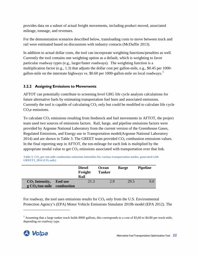
To calculate CO2 emissions resulting from feedstock and fuel movements in AFTOT, the project team used two sources of emissions factors. Rail, barge, and pipeline emissions factors were provided by Argonne National Laboratory from the current version of the Greenhouse Gases, Regulated Emissions, and Energy use in Transportation model(Argonne National Laboratory 2014) and are shown in Table 3. The GREET team provided CO2 combustion emissions values. In the final reporting step in AFTOT, the ton-mileage for each link is multiplied by the appropriate modal value to get CO2 emissions associated with transportation over that link.
Table 3: CO2 per ton-mile combustion emissions intensities for various transportation modes, generated with GREET1_2014 (CO2 only)
Diesel Freight Rail
Ocean Tanker
Barge Pipeline
CO2 Intensity, g CO2/ton-mile
End use combustion
21.3 2.9 29.5 0.0
For roadway, the tool uses emissions results for CO2 only from the U.S. Environmental Protection Agency’s (EPA) Motor Vehicle Emissions Simulator 2010b model (EPA 2012). The
3 Assuming that a large tanker truck holds 8000 gallons, this corresponds to a cost of $3,60 to $4.80 per truck-mile, depending on roadway type.
Alternative Fuel Transportation Optimization Tool 22
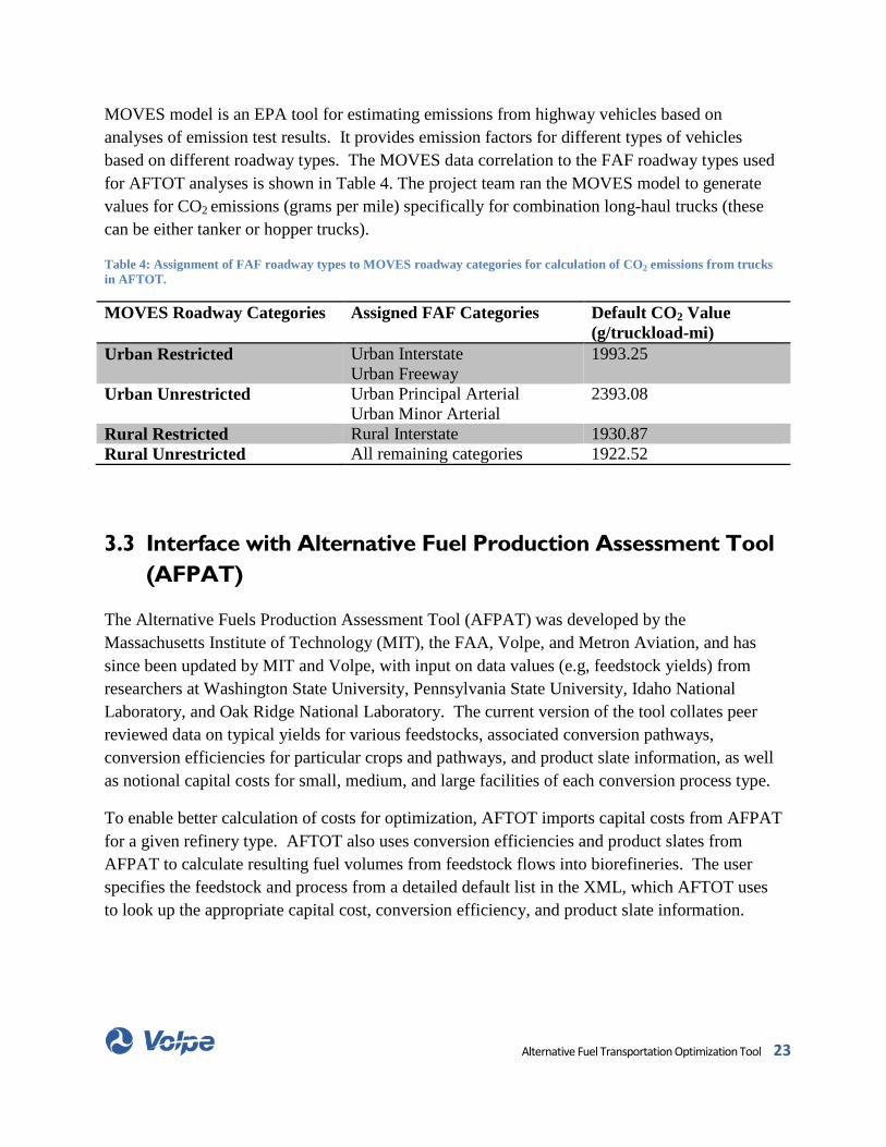
MOVES model is an EPA tool for estimating emissions from highway vehicles based on analyses of emission test results. It provides emission factors for different types of vehicles based on different roadway types. The MOVES data correlation to the FAF roadway types used for AFTOT analyses is shown in Table 4. The project team ran the MOVES model to generate values for CO2 emissions (grams per mile) specifically for combination long-haul trucks (these can be either tanker or hopper trucks).
Table 4: Assignment of FAF roadway types to MOVES roadway categories for calculation of CO2 emissions from trucks in AFTOT.
MOVES Roadway Categories Assigned FAF Categories Default CO2 Value (g/truckload-mi)
Urban Restricted Urban Interstate Urban Freeway
1993.25
Urban Unrestricted Urban Principal Arterial Urban Minor Arterial
2393.08
Rural Restricted Rural Interstate 1930.87 Rural Unrestricted All remaining categories 1922.52
3.3 Interface with Alternative Fuel Production Assessment Tool (AFPAT)
The Alternative Fuels Production Assessment Tool (AFPAT) was developed by the Massachusetts Institute of Technology (MIT), the FAA, Volpe, and Metron Aviation, and has since been updated by MIT and Volpe, with input on data values (e.g, feedstock yields) from researchers at Washington State University, Pennsylvania State University, Idaho National Laboratory, and Oak Ridge National Laboratory. The current version of the tool collates peer reviewed data on typical yields for various feedstocks, associated conversion pathways, conversion efficiencies for particular crops and pathways, and product slate information, as well as notional capital costs for small, medium, and large facilities of each conversion process type.
To enable better calculation of costs for optimization, AFTOT imports capital costs from AFPAT for a given refinery type. AFTOT also uses conversion efficiencies and product slates from AFPAT to calculate resulting fuel volumes from feedstock flows into biorefineries. The user specifies the feedstock and process from a detailed default list in the XML, which AFTOT uses to look up the appropriate capital cost, conversion efficiency, and product slate information.
Alternative Fuel Transportation Optimization Tool 23

3.4 GIS route identification step
Once all the data have been fed into the tool via the GIS layers and network generation, the XML, and the interface with AFPAT, the GIS module then identifies the routes and costs from preprocessors to biorefineries, and then from biorefineries to destinations. For each origin-and-destination (OD) pair, the GIS module uses the values above to calculate all possible route (and intermodal) combinations and then identifies the route with the lowest overall cost. The GIS passes these routes and candidate biorefinery locations to the PuLP optimizer, which resolves how much material should flow along which routes and to which biorefineries and final destinations (e.g., airports) to minimize the total cost of transportation from each preprocessor to the final fuel destination(s).
3.5 Optimization tools and methods
3.5.1 PuLP optimizer – problem definition
The PuLP optimizer is a Python-based tool that identifies a maximum or minimum value (in this case, minimizing total cost and weighting) using a mathematical description of the problem at hand. In its application for AFTOT, the PuLP optimizer takes all of the origins (and crop production information), destinations (and fuel demand information), waypoints, list of candidate biorefinery locations, and the transportation network as defined by the GIS module (described in Section 3.1) and optimizes the paths among all components. This optimization includes recommended biorefinery locations taken from the candidate list. The goal of the optimization is to minimize the total annual “cost” of meeting as much fuel demand as possible by utilizing multiple fuel-producing crops and transportation modes. The “cost” in the optimization includes not only actual dollar costs of transporting the material, but also weightings and penalties that force the tool to favor particular desirable characteristics of the routing. This analysis included factors for:
1) Actual transportation costs (as outlined in Section 3.2.1) a. Mode specific transport costs b. Transloading costs
2) Capital costs a. Amortized annual capital expenses for biorefinery construction (from
AFPAT) 3) Weightings and penalties
Alternative Fuel Transportation Optimization Tool 24

a. Roadway type. The preference for different roadway types is achieved by assigning varying dollar costs per gallon-mile.
b. Unmet demand penalty: each destination has a desired quantity of fuel to receive annually. For every thousand gallons of demand not met during the scenario timeframe (total, for all destinations and fuel types) the optimization adds a penalty to the cost of that “solution;” the magnitude of this penalty is configurable as part of the optimization, so that one can prioritize transportation costs versus the possibility of not meeting all demand. This penalty is required for the optimizer to function; if there is no penalty for not meeting demand, the lowest cost solution is always to transport nothing at all. In general, it may be necessary to raise this penalty when any other cost (e.g. rail transport) is raised, or else the optimizer will conclude that it is more optimal to transport less material. As a general guide, the unmet demand penalty works best if set to be 10-50 times the average actual transportation cost. This ensures that feedstock and fuel will be transported even over long routes. A very low unmet demand penalty may result in little or no flow as transportation costs exceed the penalty, whereas an excessively high unmet demand penalty may force the flow of materials. The tool includes a mechanism to estimate the unmet demand penalty based on the scenario demand, maximum feedstock transport distance, and assuming the highest cost mode of transport. The estimate provides a lower limit on the demand penalty, but the user may wish to increase the penalty to ensure that the tool will be driven to flow material.
c. Minimum flow requirements: for a biorefinery to be used, it must process at least a certain amount of feedstock (minimum provided by the user). For a preprocessor to be included, it must produce enough crop to create a certain annual amount of feedstock as specified by the user.
These costs and weightings are translated to mathematical decision variables and coefficients as follows in Table 5.
Alternative Fuel Transportation Optimization Tool 25
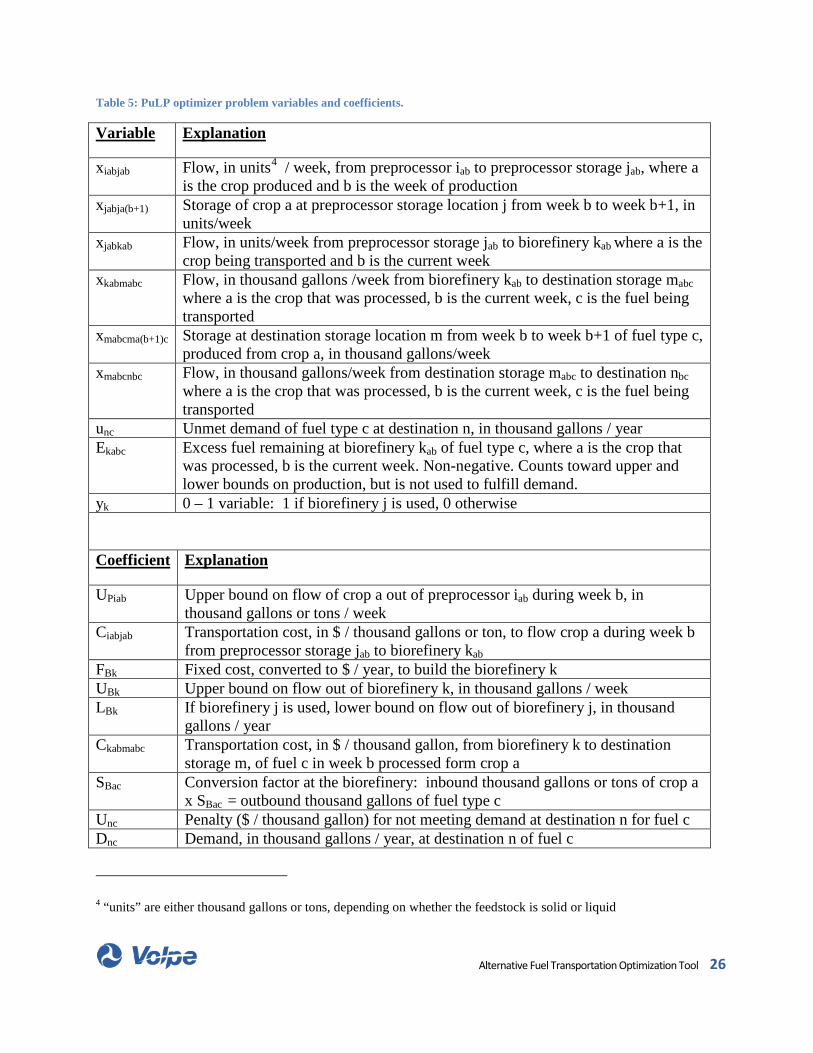
Table 5: PuLP optimizer problem variables and coefficients.
Variable Explanation
xiabjab Flow, in units4 / week, from preprocessor iab to preprocessor storage jab, where a is the crop produced and b is the week of production
xjabja(b+1) Storage of crop a at preprocessor storage location j from week b to week b+1, in units/week
xjabkab Flow, in units/week from preprocessor storage jab to biorefinery kab where a is the crop being transported and b is the current week
xkabmabc Flow, in thousand gallons /week from biorefinery kab to destination storage mabc where a is the crop that was processed, b is the current week, c is the fuel being transported
xmabcma(b+1)c Storage at destination storage location m from week b to week b+1 of fuel type c, produced from crop a, in thousand gallons/week
xmabcnbc Flow, in thousand gallons/week from destination storage mabc to destination nbc where a is the crop that was processed, b is the current week, c is the fuel being transported
unc Unmet demand of fuel type c at destination n, in thousand gallons / year Ekabc Excess fuel remaining at biorefinery kab of fuel type c, where a is the crop that
was processed, b is the current week. Non-negative. Counts toward upper and lower bounds on production, but is not used to fulfill demand.
yk 0 – 1 variable: 1 if biorefinery j is used, 0 otherwise Coefficient Explanation
UPiab Upper bound on flow of crop a out of preprocessor iab during week b, in thousand gallons or tons / week
Ciabjab Transportation cost, in $ / thousand gallons or ton, to flow crop a during week b from preprocessor storage jab to biorefinery kab
FBk Fixed cost, converted to $ / year, to build the biorefinery k UBk Upper bound on flow out of biorefinery k, in thousand gallons / week LBk If biorefinery j is used, lower bound on flow out of biorefinery j, in thousand
gallons / year Ckabmabc Transportation cost, in $ / thousand gallon, from biorefinery k to destination
storage m, of fuel c in week b processed form crop a SBac Conversion factor at the biorefinery: inbound thousand gallons or tons of crop a
x SBac = outbound thousand gallons of fuel type c Unc Penalty ($ / thousand gallon) for not meeting demand at destination n for fuel c Dnc Demand, in thousand gallons / year, at destination n of fuel c
4 “units” are either thousand gallons or tons, depending on whether the feedstock is solid or liquid
Alternative Fuel Transportation Optimization Tool 26

Then the problem for AFTOT analysis is mathematically stated as follows:
Minimize annual cost = ∑jabkab Cjabkab xjabkab + ∑k (FBk yk )+ ∑kabmabc Ckabmabc xkabmabc + ∑nc (Unc unc)
Subject to the following constraints show in Table 6.
Table 6: PuLP Optimizer Constraints
Constraint Explanation (1) For each biorefinery kab, SBac ∑ jabkab xjabkab - ∑ kabmabc xkabmabc = Ekabc
Flow must be conserved at each stage relative to time, crop, and fuel type (with the appropriate conversion factors) ; any excess is tracked.
(2) For each biorefinery kab, yk UBk - ∑kabmabc xkabmabc - Ekabc ≥ 0
If a biorefinery is used, flow cannot exceed the upper bound during any week, across all crops and fuel types, including excess. Note that if the biorefinery is not used (yj = 0), this constraint requires the flow into the biorefinery be 0.
(3) For each biorefinery kab, yk LBk - ∑ kabmabc xkabmabc - Ekabc ≤ 0
If a biorefinery is used, the flow out of it over a year must exceed the lower bound, summing all crops and fuel types.
(4) For each preprocessor iab, ∑ iabjab xiabjab ≤ UPiab
Flow out of each preprocessor does not exceed the preprocessor upper bound, for each week and crop
(5) For each destination nc, ∑ mabcnbc xmabcnbc + unc = Dnc
Unmet demand plus flow into a destination is equal to that destination’s demand, for each fuel type
(6) The y variables are binary (0 or 1) A biorefinery is used, or it isn’t. (7) The x, E, and u variables are non-negative No negative flows are permitted
The PuLP optimizer takes in the various options for building routes between origins and destinations from the GIS module. The optimizer then uses standard linear optimization techniques such as a revised simplex algorithm to solve the mathematical description of the problem to move material from origin to destination by selecting among paths and biorefinery options for each unit of feedstock or fuel. The specific choice of algorithm is made by the COINMP_DLL solver, as implemented by PuLP. The allocation of crops and fuel among routes, biorefineries, and destinations is based on meeting maximum demand while minimizing the total cost, without violating the constraints on minimum and maximum flow.
Alternative Fuel Transportation Optimization Tool 27

3.6 Reporting Outputs
Once the optimization is complete, the GIS module takes the data generated by the optimizer and develops maps and spreadsheet data reports. The spreadsheet data report lists all of the xml input parameters, the source data, the version of AFTOT used, the preliminary calculations done by AFTOT, interim results, and final outputs for cost, mileage, vehicle miles traveled, number of loads, and CO2 emissions. It also reports the destinations, the amount of demand fulfilled, and the total demand fulfilled for the scenario. Additional outputs can include information aggregated for a given biorefinery or destination, or by route.
3.7 Map Outputs
For each scenario, AFTOT also generates a multilayered GIS map (see example in Figure 7) that shows:
• Preprocessor locations are located at the centroid of a county. Preprocessors used in the optimal solution are presented by a green circle.
• Biorefinery locations used in the optimal solution are represented by an orange circle.
• Destinations, such as DFSPs and airports, used in the optimal solution are represented by a brown circle”. Airports are labeled with their three letter code as used throughout the aviation sector. DFSPs are labeled with their city/town of location.
• Intermodal facilities (not shown) are represented by a pink circle. There are 383 intermodal facilities which can obscure the routes and locations of preprocessor, biorefineries, and destinations and are not displayed by default, although this layer can be turned on if needed.
• The network segments used in the optimized solution are shown. Each mode in the optimized solution is represented by a dark color:
o Water – blue o Pipeline – black – NOTE: pipeline has been represented by a manually
drawn straight line between approximate origins and destinations on the graphics presented herein due to restrictions on geospatial representation of pipeline. Actual network data were used to calculate routes and costs
o Rail - pink o Road - red
Each of these layers can be turned on and off to facilitate visual exploration of the results.
Alternative Fuel Transportation Optimization Tool 28

Figure 7: Example map output from an AFTOT scenario visualizing the scenario results and demonstrating symbology. Pipeline in this map is an overlain straight line between selected origins and destinations and does not reflect underlying geospatial network data used in the calculations for the analysis.
3.8 Testing and Verification of Model Functions
The team performed a variety of tests on model performance as part of model development to ensure that the tool executes its calculations and optimization properly and that the tool’s modules are internally consistent with one another. When using two different software tools, one must exercise particular care to ensure that nothing is lost in the transfer of data among units of the model. The following tests and verification procedures were used to ensure the accuracy and performance of the tool and the validity of the results:
1) During coding, a logging process was implemented to track performance time for various steps and check interim calculations in the model. Files produced by the program included
• A logfile for each processing step and individual timestamps for each subroutine in the process.
• A logfile of assumptions (parameter settings) for that particular scenario.
Alternative Fuel Transportation Optimization Tool 29

• A human and machine readable file of the mixed integer optimization problemthat is solved by the PuLP optimization, listing all variables, constraints andcoefficients.
• A human and machine readable file of the solution (values of each variable)produced by the optimization.
2) The team performed detailed end-to-end audits of a small number of routes withinexecuted scenarios, where the total flow of material and transportation / transloadingcosts were calculated by hand for individual links in the network and then checkedagainst the reported totals in the model outputs. The hand-calculated transportation costsfor selected routes were also compared with the GIS module’s calculated routetransportation costs that were fed into the PuLP optimization to ensure correct transfer ofinformation between modules at both the beginning and end of the optimization process.
3) For selected scenarios, the team compared the output reports with each other and with thedetailed mixed integer program solution produced by PuLP, to ensure internalconsistency and correct transfer of information between PuLP and GIS after theoptimization.
4) After code was finalized, the same scenarios were run on multiple machines and bymultiple people to check for consistency and stability of the tool. Scenario results cameout identically on different machines.
3.9 Known Issues and Limitations
As with any software tool under ongoing development, AFTOT has known bugs and limitations, which are briefly summarized here.
1) Pipeline – currently the tool contains approximately 75% of the OD pairs that exist in the pipeline systems. Phase 3 development will entail completion of the full pipeline system in the network.
2) Pipeline – certain included pipeline routes do not contain base rate data and thereforecosts associated with movements along these routes are not currently included in overallcost or per gallon cost estimates for scenarios that use them. These will be updated inPhase 3 as well.
3) Pipeline – in rare cases in which feedstock production occurs within 5 miles of an originpoint in the pipeline database, an artificial link may be created that would erroneouslyallow feedstock to flow over pipeline. While the distances involved under suchcircumstances are very small, this can introduce a small additional error into the finalcalculations. This issue will be addressed in Phase 3.
Alternative Fuel Transportation Optimization Tool 30
4) Zero-flow solution / No optimal solution found – in some cases AFTOT will return the error “no optimal solution found” even with a properly specified scenario. In this case, PuLP calculates the lowest cost option is to have zero-flow over the network. The following variables can be adjusted in the scenario XML configuration file in order to force flow: lowering the cost and/or size of biorefineries, increasing destination demand, increasing biomass production, increasing unmet demand penalty.
5) Single pathway scenarios – currently the tool can address one biorefinery type in a given scenario (e.g., pyrolysis or HEFA or Fischer-Tropsch). Therefore, for complex scenarios involving more than one pathway type, the user must run a scenario for each pathway/feedstock combination and collate the results at the end. In cases where demand centers are shared, this means that the user must either allocate demand among pathways in advance or prioritize pathways and adjust demand downward for each successive run until the demand centers are filled. An approach to managing this internally will be investigated in Phase 3.
Alternative Fuel Transportation Optimization Tool 31

4 Demonstration of Model Capabilities Six scenarios were selected to demonstrate the capabilities of AFTOT to identify optimal transportation patterns based on factors that are likely to be of interest to potential users of the tool. The three test scenarios (Test Scenarios 1-3) described below demonstrate the capabilities of the tool, increasing from a single origin, destination, and biorefinery in a geographic scale covering a couple of counties (Test Scenario 1) to a Gulf Coast regional scale showing local pipeline integration (Test Scenario 2) to a Gulf Coast regional scale extending up the East Coast demonstrating greater pipeline integration (Test Scenario 3).
The full scenarios (Scenario 4-6) were defined based on discussions with FAA. Scenario 4 analyzes the downstream transportation and refining optimization based on a USDA break-even analysis for oilseed production. The scenario presented herein uses first-run dataset for North Dakota and delivers the resulting HEFA fuels to airports and DFSPs. Scenario 5 demonstrates the ability to use existing materials such as crop residues (e.g., wheat straw) in the most efficient processing option for that feedstock (advanced fermentation) and deliver the resulting fuels to airports and DFSPs. Scenario 6 uses a highly cited biomass feedstock dataset from the DOE “Billion Ton Study Update” (Perlack and Stokes 2011) as a mixed feedstock scenario, with the feedstocks processed by the most efficient technology available and then delivered to airports and DFSPs. These scenarios are summarized in Figure 8.
For all of the scenarios described, the same default set of costs and weightings were used. These are shown in Table 5. Selected scenario level details of inputs and results are provided in Table 6 and described in the following sections.
Alternative Fuel Transportation Optimization Tool 32

Figure 8: Feedstock source, processing type, and destinations for demonstration Scenarios 5-7.
Table 7: Key input parameters common to all demonstration scenarios described in this report.
Input Parameter Value Common to Scenarios Below Trucking base cost (per 1 kgal-mi / per tonne mi) $0.45 per kgal-mi / $0.15 per tonne-mi Rail cost (per 1 kgal-mi / per tonne mi) $0.12 per kgal-mi / $0.04 per tonne-mi Barge cost (per 1 kgal-mi/ per tonne mi) $0.05 per kgal-mi / $0.0167 per tonne-mi Pipeline cost Based on OD pair tariffs Transloading cost (per 1 kgal or metric ton) $40/$13.3 Trucking interstate weighting 1 Trucking principal arterial weighting 1.10 Trucking minor arterial weighting 1.20 Trucking local weighting 1.30 Maximum artificial link distance (to join network – in miles) 5 Time steps 1 (annual results)
Alternative Fuel Transportation Optimization Tool 33
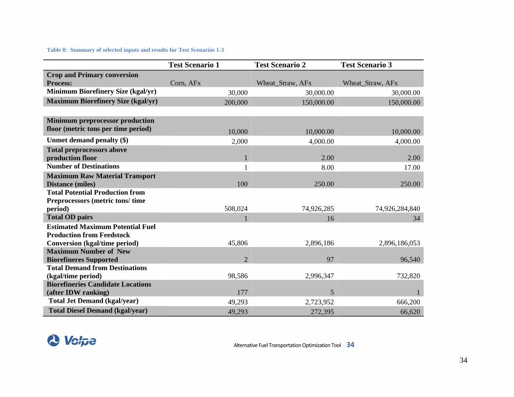
Table 8: Summary of selected inputs and results for Test Scenarios 1-3
Test Scenario 1 Test Scenario 2 Test Scenario 3 Crop and Primary conversion Process: Corn, AFx Wheat_Straw, AFx Wheat_Straw, AFx Minimum Biorefinery Size (kgal/yr) 30,000 30,000.00 30,000.00 Maximum Biorefinery Size (kgal/yr) 200,000 150,000.00 150,000.00
Minimum preprocessor production floor (metric tons per time period) 10,000 10,000.00 10,000.00 Unmet demand penalty ($) 2,000 4,000.00 4,000.00 Total preprocessors above production floor 1 2.00 2.00 Number of Destinations 1 8.00 17.00 Maximum Raw Material Transport Distance (miles)
100
250.00
250.00
Total Potential Production from Preprocessors (metric tons/ time period)
508,024
74,926,285
74,926,284,840
Total OD pairs 1 16 34 Estimated Maximum Potential Fuel Production from Feedstock Conversion (kgal/time period)
45,806
2,896,186
2,896,186,053
Maximum Number of New Biorefineres Supported 2
97
96,540
Total Demand from Destinations (kgal/time period)
98,586
2,996,347
732,820
Biorefineries Candidate Locations (after IDW ranking)
177
5
1
Total Jet Demand (kgal/year) 49,293 2,723,952 666,200 Total Diesel Demand (kgal/year) 49,293 272,395 66,620
Alternative Fuel Transportation Optimization Tool 34
34
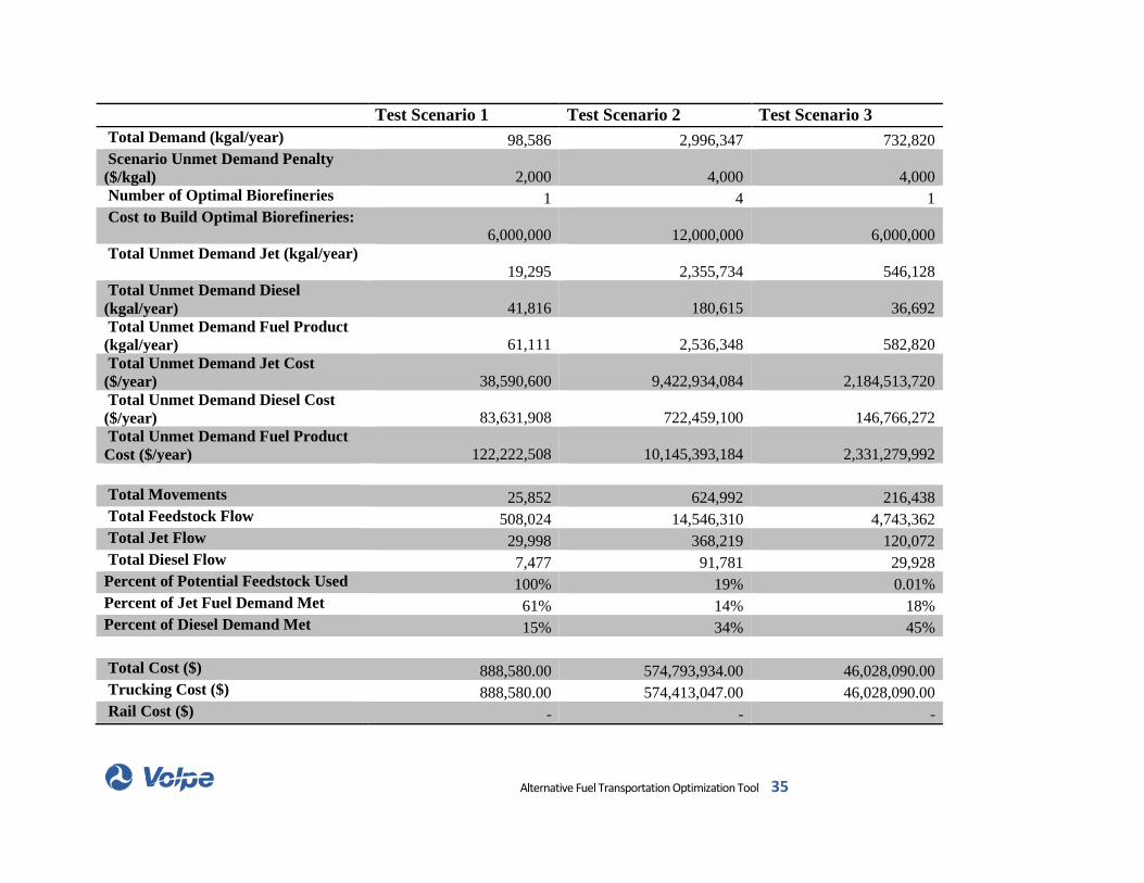
Test Scenario 1 Test Scenario 2 Test Scenario 3 Total Demand (kgal/year) 98,586 2,996,347 732,820 Scenario Unmet Demand Penalty ($/kgal)
2,000
4,000
4,000
Number of Optimal Biorefineries 1 4 1 Cost to Build Optimal Biorefineries:
6,000,000
12,000,000
6,000,000 Total Unmet Demand Jet (kgal/year)
19,295
2,355,734
546,128 Total Unmet Demand Diesel (kgal/year)
41,816
180,615
36,692
Total Unmet Demand Fuel Product (kgal/year)
61,111
2,536,348
582,820
Total Unmet Demand Jet Cost ($/year)
38,590,600
9,422,934,084
2,184,513,720
Total Unmet Demand Diesel Cost ($/year)
83,631,908
722,459,100
146,766,272
Total Unmet Demand Fuel Product Cost ($/year)
122,222,508
10,145,393,184
2,331,279,992
Total Movements 25,852 624,992 216,438
Total Feedstock Flow 508,024 14,546,310 4,743,362 Total Jet Flow 29,998 368,219 120,072 Total Diesel Flow 7,477 91,781 29,928 Percent of Potential Feedstock Used 100% 19% 0.01% Percent of Jet Fuel Demand Met 61% 14% 18% Percent of Diesel Demand Met 15% 34% 45%
Total Cost ($) 888,580.00 574,793,934.00 46,028,090.00 Trucking Cost ($) 888,580.00 574,413,047.00 46,028,090.00 Rail Cost ($) - - -
Alternative Fuel Transportation Optimization Tool 35

Test Scenario 1 Test Scenario 2 Test Scenario 3 Barge Cost ($) - - - Pipeline Cost ($) - 380,887.00 - Cost per Gallon of Fuel Delivered 0.02 1.25 0.31
Total Vehicle Miles Traveled (VMT) 89,405
47,209,961
5,658,281
Truck VMT 89,405 47,209,961 5,658,281 Railcar VMT - - - Barge VMT - - -
Truckloads 25,852 624,846 216,390 Railcar Loads - - - Barge Loads - - - Pipeline Movements - 146 48
Total Miles of Network Used 11 3,835 1,274 Road Network Miles Used 11 570 193 Rail Network Miles Used - - - Water Network Miles Used - - - Pipeline Network Miles Used - 3,265 1,081
Total CO2 Combustion Emissions 171,882,050 93,280,428,969 11,043,634,165 Total Rail CO2 Emissions - - - Total Truck CO2 Emissions 171,882,050 93,280,428,969 11,043,634,165 Total Barge CO2 Emissions - - - Total Pipeline CO2 Emissions - - -
Alternative Fuel Transportation Optimization Tool 36

4.1 Test Scenario 1 – Small geographical area test case
4.1.1 Objective
This scenario is the simplest test case of one origin, one biorefinery candidate location, one destination and one mode (road only) in a single county. The scenario demonstrates the tool’s capability to run and solve scenarios in a small geographic area, allowing for simple comprehension and rapid auditing of results. This test scenario also demonstrates the geographic scope that would be used to explore options for an individual airport, biorefinery, etc.
4.1.2 Geographical Scope
This scenario focuses on a sub-regional scope encompassing one county, one origin, one biorefinery, and one destination, allowing travel only by road (truck).
4.1.3 Key Input Parameter Values
Test Scenario 1 used a subset of the AFTOT intermodal network surrounding a particular county and airport, specifically the DFSP in Omaha, Nebraska. The feedstock data for the arbitrarily selected county came from a gridded dataset developed by MIT on future bioenergy potential with corn as a potential feedstock, but this scenario is not intended to suggest that corn is likely to be used for advanced biofuels; the feedstock data simply provide a hypothetical county production level to enable tool testing. The advanced fermentation pathway in AFPAT can be tuned to predominantly produce jet fuel. Jet fuel and diesel demand were both set at 49 million gallons per year. The biorefinery size was set at a minimum of 30 million gallons per year.
4.1.4 Run Summary
AFTOT processed Test Scenario 1 in approximately 5 minutes. Given the narrow scope of the scenario, only one route was generated. AFTOT generated two candidate biorefinery, of which one was used. Potential feedstock production was 508,024 metric tons annually, with the possibility of producing up to 45.8 million gallons of fuel products per year.
Alternative Fuel Transportation Optimization Tool 37
37

4.1.5 Results/Conclusions
In Test Scenario 1, 100% of the potential feedstock production (508,024 metric tons) was used to make fuel in the single candidate biorefinery location selected during the optimization by AFTOT. This amount of feedstock produced 30 million gallons of jet fuel and 7.5 million gallons of diesel.
The total cost to move this material was $51,500 to move nearly 26,000 truckloads over 89,405 vehicle miles. All of those vehicle miles traveled (VMT) occurred on only 11 miles of roadway. The average per gallon cost of moving the fuels was approximately $0.02 per gallon, which is low because of the very short distances involved. This produced 172 metric tons of CO2.
Figure 9: Map of Test Scenario 1 showing single origin, biorefinery and destination and demonstrating ability of AFTOT to perform a simple, geographically constrained analysis.
Alternative Fuel Transportation Optimization Tool 38

4.2 Test Scenario 2 – Regional geographical area test (Gulf Coast)
4.2.1 Objective
Test Scenario 2 demonstrates the tool’s capability to run and solve scenarios in a mid-sized/regional geographic area, such as an analysis of a few closely spaced biorefineries and/or delivery to a few airports in one or several states. This scenario also verifies pipeline network integration. It includes roadway and pipeline modes to ensure travel over pipeline and verify connectivity and performance.
4.2.2 Geographical Scope
Test Scenario 2 focuses on the Gulf Coast region. The road network within approximately a 200-mile radius of Houston is included. The entire pipeline network is also included.
4.2.3 Key Parameter Values
Test Scenario 2 uses a small geographic subset of the USDA NASS wheat straw data, which is converted to fuels by advanced fermentation (AFx), as this is the most efficient conversion technology AFPAT identifies for this feedstock. The advanced fermentation pathway (conventional fermentation to ethanol with dilute acid pretreatment), in AFPAT predominantly produces jet fuel through an ethanol oligomerization process. The unmet demand penalty was set at $4,000 per thousand gallons.
4.2.4 Run Summary
AFTOT processed Test Scenario 2 in approximately 25 minutes. Two preprocessors and eight destinations were included, leading to 16 original OD pairs. Seven candidate biorefinery locations were generated, of which two were eliminated by IDW weighting. Potential feedstock production was almost 75 million metric tons, which could support up to 97 biorefineries using AFx conversion with a minimum production floor of 30,000 kgal/year, resulting in total potential fuel production (diesel, jet, naptha, etc.) of 2.9 billion gallons of fuel. Jet fuel demand was set at 2.7 billion gallons per year, diesel at 272 million gallons.
Alternative Fuel Transportation Optimization Tool 39

4.2.5 Results/Conclusions
In Test Scenario 2, 19% (14.5 million metric tons) of the potential feedstock production was used to make fuel in the four candidate biorefinery locations selected by AFTOT in the optimization. This amount of feedstock produced 368 million gallons of jet fuel and 92 million gallons of diesel. This met about 14% of the jet fuel demand and about 34% of the diesel demand designated in the scenario for all potential destinations, demonstrating the tool’s balancing of feedstock use/fuel production against the cost of “doing nothing” and paying the unmet demand penalty. The resulting fuel was delivered by pipeline to the Dallas-Fort Worth Airport (DFW), Atlanta Airport (ATL) and Ronald Reagan National Airport (DCA), with the initial transfer by truck from the biorefinery site not located at the pipeline. For DFW, ATL, and DCA, 31%, 71% and 0% of jet fuel demand and 78%, 100% and 15% of diesel demand were met, respectively, for a total fulfillment of 11% of jet fuel demand and 27% of diesel demand overall.
The total cost to move this material was $574 million, all of which was associated with the transport of fuel, as the biorefinery was essentially co-located with feedstock production. The per unit cost of moving the fuel was approximately $1.25 per gallon. However, this value is an underestimate, as some pipeline movements contained in this scenario did not have a base rate value in the tariff data and therefore were set to zero. Further development will include attempts to resolve zero-value movements. It would take approximately 625,000 truckloads traveling 47 million vehicle miles over 1835 miles of roadway for transport of the fuel. In addition, 3,265 miles of pipeline were used for 146 pipeline movements. The CO2 emitted was approximately 93,000 metric tons.
Alternative Fuel Transportation Optimization Tool 40

Figure 10: Map of Test Scenario 2 demonstrating AFTOT ability to perform a mid-size geographic scope analysis, including utilization of pipeline. Note that pipeline routes are represented by a straight line connecting origins and destinations and do not reflect actual geospatial data on pipeline location, although actual network data are used to run the scenario and identify routing options.
.
4.3 Test Scenario 3 – Broad regional scenario test
4.3.1 Objective
Test Scenario 3 is similar to Test Scenario 2 in that this scenario demonstrates AFTOT’s capability to run and solve scenarios integrating pipeline and testing wheat straw conversion via AFx to jet and diesel fuel. This scenario removed the destinations closets to the biorefineries in Test Scenario 2 to expand the geographic extent of the pipeline network as a larger test of the flowable pipeline network, and, provides a broader perspective on potential movements based on
Alternative Fuel Transportation Optimization Tool 41

transport cost. The road network within approximately a 200-mile radius of Houston is included. The entire pipeline network is also included. To ensure the scenario was not constrained on the feedstock supply, the agricultural layer was updated to include one thousand times more material than Test Scenario 2, but uses the same counties.
4.3.2 Geographical Scope
Test Scenario 3 covers the eastern U.S., with feedstock production and transport focused on the Gulf Coast region, and allow demand to be met throughout the Midwestern and Eastern U.S. based on transport over pipeline.
4.3.3 Key Parameter Values
As with Test Scenario 2, Test Scenario 3 uses a small geographic subset of the USDA NASS wheat straw data, which is converted to fuels by advanced fermentation (AFx), as this is the most efficient conversion technology AFPAT identifies for this feedstock. The advanced fermentation pathway in AFPAT can be tuned to predominantly produce jet fuel. As stated earlier, the county yield is increased by a factor of 1,000 to remove feedstock supply constraints. The unmet demand penalty was set at $4,000 per thousand gallons.
4.3.4 Run Summary
AFTOT processed Test Scenario 3 in approximately 39 minutes. Two preprocessors and 17 destinations were included, leading to 34 original OD pairs. Two candidate biorefinery locations were generated, but one was eliminated by the IDW process. Potential feedstock production was 1,000 times that of Test Scenario 2 (75 billion metric tons) in order to drive the scenario production higher and thereby test the further transport along the pipeline network. This amount of feedstock could hypothetically support nearly 97,000 biorefineries using AFx conversion with a minimum production floor of 30,000 kgal/year, resulting in total potential fuel production (diesel, jet, naptha, etc.) of 2.9 trillion gallons of fuel (again, these results are 1,000 higher due to increased production at the preprocessor for this test). In this scenario, jet fuel demand was 666 million gallons per year and diesel demand was set at 10% of jet fuel demand (66 million gallons per year). This demand is 25% of the demand in Test Scenario 2 due to the elimination of large Southeastern airports (e.g. ATL, DFW) to drive pipeline use in the scenario optimization.
4.3.5 Results/Conclusions
Alternative Fuel Transportation Optimization Tool 42

In Test Scenario 3, only 0.01% (4.7 million metric tons) of the potential feedstock production was used to make fuel in the one candidate biorefinery location identified as the optimal solution by AFTOT. This amount of feedstock produced 120 million gallons of jet fuel and 30 million gallons of diesel. This met about 18% of the total jet fuel demand and about 45% of the diesel demand designated in the scenario for all destinations. All of this fuel was delivered to Dulles International Airport (IAD) in the Washington, DC region, at which 26.% of jet fuel demand and 65% of diesel demand were met. The total amount of fuel produced in this scenario is less than that produced in Test Scenario 2 in spite of the higher feedstock production due to the further distance travel required for the fuel to reach its final destination. The tool calculates the optimization by comparing movement cost to the “no movement” cost driven by the unmet demand penalty, cost to build biorefineries, cost of moving feedstock, and penalties and weightings.
The total cost to move this material was $46 million, all of which was associated with the transport of fuel, as the biorefinery was essentially co-located with feedstock production. The per unit cost of moving the fuel was approximately $0.31 per gallon. Moving this fuel required 216,400 truck loads and 5.7 million miles of truck travel, covering 193 miles of roadway. However most of the transport was on the pipeline, covering 1,100 miles of the pipeline network. All CO2 was associated with truck movements and totaled 1,100 metric tons.
Alternative Fuel Transportation Optimization Tool 43

Figure 11: Map of Test Scenario 3 showing national scale test scenario processing wheat straw into jet fuel and diesel and transporting over a network including all modes. Note that pipeline routes are represented by a straight line connecting origins and destinations and do not reflect actual geospatial data on pipeline location, although actual network data are used to run the scenario and identify routing options.
Alternative Fuel Transportation Optimization Tool 44
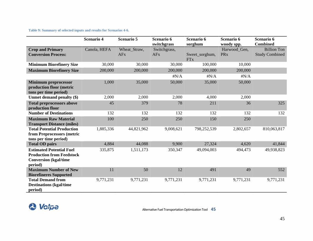
Table 9: Summary of selected inputs and results for Scenarios 4-6.
Scenario 4 Scenario 5 Scenario 6 switchgrass
Scenario 6 sorghum
Scenario 6 woody spp.
Scenario 6 Combined
Crop and Primary Conversion Process:
Canola, HEFA Wheat_Straw, AFx
Switchgrass, AFx
Sweet_sorghum, FTx
Harwood_Gen, PRx
Billion Ton Study Combined
Minimum Biorefinery Size 30,000 30,000 30,000 100,000 10,000 Maximum Biorefinery Size 200,000 200,000 200,000 200,000 200,000 #N/A #N/A #N/A Minimum preprocessor production floor (metric tons per time period)
1,000 35,000 50,000 35,000 50,000
Unmet demand penalty ($) 2,000 2,000 2,000 4,000 2,000 Total preprocessors above production floor
45 379 78 211 36 325
Number of Destinations 132 132 132 132 132 132 Maximum Raw Material Transport Distance (miles)
100 250 250 150 250
Total Potential Production from Preprocessors (metric tons per time period)
1,885,336 44,821,962 9,008,621 798,252,539 2,802,657 810,063,817
Total OD pairs 4,884 44,088 9,900 27,324 4,620 41,844 Estimated Potential Fuel Production from Feedstock Conversion (kgal/time period)
335,875 1,511,173 350,347 49,094,003 494,473 49,938,823
Maximum Number of New Biorefineres Supported
11 50 12 491 49 552
Total Demand from Destinations (kgal/time period)
9,771,231 9,771,231 9,771,231 9,771,231 9,771,231 9,771,231
Alternative Fuel Transportation Optimization Tool 45
45
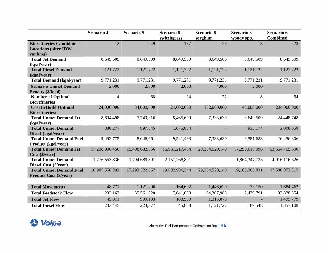
Scenario 4 Scenario 5 Scenario 6 switchgrass
Scenario 6 sorghum
Scenario 6 woody spp.
Scenario 6 Combined
Biorefineries Candidate Locations (after IDW ranking)
12 249 187 23 13 223
Total Jet Demand (kgal/year)
8,649,509 8,649,509 8,649,509 8,649,509 8,649,509 8,649,509
Total Diesel Demand (kgal/year)
1,121,722 1,121,722 1,121,722 1,121,722 1,121,722 1,121,722
Total Demand (kgal/year) 9,771,231 9,771,231 9,771,231 9,771,231 9,771,231 9,771,231 Scenario Unmet Demand Penalty ($/kgal)
2,000 2,000 2,000 4,000 2,000
Number of Optimal Biorefineries
4 68 24 22 8 54
Cost to Build Optimal Biorefineries:
24,000,000 84,000,000 24,000,000 132,000,000 48,000,000 204,000,000
Total Unmet Demand Jet (kgal/year)
8,604,498 7,749,316 8,465,609 7,333,630 8,649,509 24,448,748
Total Unmet Demand Diesel (kgal/year)
888,277 897,345 1,075,884 - 932,174 2,008,058
Total Unmet Demand Fuel Product (kgal/year)
9,492,775 8,646,661 9,541,493 7,333,630 9,581,683 26,456,806
Total Unmet Demand Jet Cost ($/year)
17,208,996,456 15,498,632,856 16,931,217,454 29,334,520,140 17,299,018,096 63,564,755,690
Total Unmet Demand Diesel Cost ($/year)
1,776,553,836 1,794,689,801 2,151,768,891 - 1,864,347,735 4,016,116,626
Total Unmet Demand Fuel Product Cost ($/year)
18,985,550,292 17,293,322,657 19,082,986,344 29,334,520,140 19,163,365,831 67,580,872,315
Total Movements 48,771 1,121,206 164,692 1,446,620 73,150 1,684,462 Total Feedstock Flow 1,293,162 35,561,620 7,041,080 84,307,983 2,479,791 93,828,854 Total Jet Flow 45,011 900,193 183,900 1,315,879 - 1,499,779 Total Diesel Flow 233,445 224,377 45,838 1,121,722 189,548 1,357,108
Alternative Fuel Transportation Optimization Tool 46

Scenario 4 Scenario 5 Scenario 6 switchgrass
Scenario 6 sorghum
Scenario 6 woody spp.
Scenario 6 Combined
Percent of Potential Feedstock Used
69% 79% 78% 11% 88% 12%
Percent of Jet Fuel Demand Met
1% 10% 2% 15% 0% 17%
Percent of Diesel Demand Met
21% 20% 4% 100% 17% 121%
Total Cost ($) 49,505,590.00 685,440,469.00 132,621,307.00 342,803,005.00 47,585,906.00 523,010,218.00 Trucking Cost ($) 17,697,099.00 474,452,716.00 70,507,702.00 160,569,707.00 26,332,243.00 257,409,652.00 Rail Cost ($) 22,330,259.00 202,917,834.00 55,372,500.00 147,309,676.00 19,567,649.00 222,249,825.00 Barge Cost ($) 8,223,886.00 6,727,424.00 6,741,106.00 32,480,677.00 1,522,688.00 40,744,471.00 Pipeline Cost ($) 1,254,345.00 1,342,495.00 - 2,442,945.00 163,326.00 2,606,271.00 Cost per Gallon of Fuel Delivered ($)
0.18 0.61 0.58 0.14 0.25 0.18
Total Vehicle Miles Traveled (VMT)
8,031,296 69,117,909.00 11,921,277 47,786,815 5,071,443 64,779,535
Truck VMT 1,740,675 40,010,968 5,737,314 16,545,750 2,350,189 24,633,253 Railcar VMT 6,212,298 29,028,574 5,995,734 30,660,985 2,706,472 39,363,191 Barge VMT 78,323 78,367 188,229 580,079 14,783 783,091 Truckloads 29,989 772,559 97,989 726,313 47,610 871,912 Railcar Loads 18,684 347,908 65,066 695,517 25,415 785,998 Barge Loads 75 660 1,627 24,737 121 26,485 Pipeline Movements 22 79 10 54 4 68 Total Miles of Network Used
47,299 98,559 14,630 83,053 11,309
Road Network Miles Used 1,435 10,519 1,492 3,190 775
Alternative Fuel Transportation Optimization Tool 47

Scenario 4 Scenario 5 Scenario 6 switchgrass
Scenario 6 sorghum
Scenario 6 woody spp.
Scenario 6 Combined
Rail Network Miles Used 22,793 55,748 10,320 46,952 6,685 Water Network Miles Used
21,813 22,522 2,764 30,537 3,742
Pipeline Network Miles Used
1,259 9,770 53 2,374 107
Total CO2 Combustion Emissions
28,132,042,476 141,494,325,763 27,316,133,527 126,846,789,427 12,133,482,603 166,296,405,557
Total Rail CO2 Emissions 10,853,542,050 53,464,711,208 11,418,266,708 54,602,459,761 5,002,856,410 71,023,582,879 Total Truck CO2 Emissions
3,352,993,515 77,421,882,705 11,283,066,305 32,088,281,774 4,567,664,960 47,939,013,039
Total Barge CO2 Emissions
13,925,506,912 10,607,731,850 4,614,800,514 40,156,047,892 2,562,961,233 47,333,809,639
Total Pipeline CO2 Emissions
- - - - - -
Alternative Fuel Transportation Optimization Tool 48

4.4 Scenario 4 – Oilseed Breakeven Scenario in North Dakota
4.4.1 Objective
Scenario 4 focuses on evaluating the downstream transportation patterns, costs, and CO2 emissions associated with a particular break-even analysis on oilseed production in wheat-growing areas, followed by HEFA processing and delivery to commercial airports and DFSPs. The USDA Agricultural Research Service developed a break-even profitability modeling approach that is used to estimate the oilseed price level at which the profitability of growing oilseeds becomes more profitable than growing other annual crops. The approach utilizes the EPIC (Environmental Policy Integrated Climate) model to simulate crop yields under varying weather conditions for each Soil Survey Geographic Database (SSURGO) soil map unit within the U.S. western wheat producing areas. Predominant crops and crop sequences are identified for each county in the region, and these are matched with management files from the USDA-NRCS management operations database. These management files are used to construct enterprise budgets and also the management inputs for the EPIC model. Each management system is modeled for each cultivated soil map unit within each county. Net returns are calculated for each cropping system on each soil map unit, and the system with highest estimated net returns is selected as the optimum on each soil. Management files and enterprise budgets are also constructed for each fuel oilseed (initially fuel rapeseed) grown in sequence with wheat. Net returns are estimated for each fuel oilseed cropping system over a range of fuel oilseed prices. Fuel oilseed system net returns at each price level are compared to the optimum system excluding fuel oilseeds to determine the overall optimum system at each fuel oilseed price level. This is used to estimate the area and quantity of fuel oilseed produced at each price level, and resulting natural resource impacts including soil erosion, soil organic carbon, nutrient runoff and leaching, fertilizer and fuel use. Enterprise budgets are based on 2104 input costs and 2010-2014 average crop prices. (Archer, USDA ARS, pers. comm.). As of August 2015, USDA has provided break-even data for three crop management zones in North Dakota as a preliminary dataset preceding release of a full canola break-even dataset focused on the entire upper Midwest wheat belt. Therefore, this scenario focuses on North Dakota break even data for canola in North Dakota (at a $600 price point) and delivers the resulting HEFA fuels to commercial airports and DFSPs across the country as determined by the optimization. The AFTOT team will provide the resulting CO2 emissions to Michigan Institute of Technology (MichiganTech) for use in calculating life cycle GHG emissions associated with the jet fuel resulting from this scenario. Summary information for Scenarios 4-6 are presented in Table 7.
This scenario is performed in collaboration with USDA’s Agricultural Research Service.
4.4.2 Geographical Scope
Biofuel Transportation Analysis Tool 49

This scenario focuses on canola production in the North Dakota as a test dataset for future analysis of the entire upper Midwest (the wheat belt), as defined in the ONR- and NIFA-funded study at USDA’s Agricultural Research Service (and collaborators). The data were provided at 9x9 kilometer grid scale, which was then aggregated to county level production. In cases where a grid cell was split between two or more counties, production was allocated proportionally by area to the appropriate counties.
4.4.3 Key Parameter Values
This scenario includes a minimum biorefinery capacity of 30 million gallons per year and a maximum of 200 million gallons per year. The unmet demand penalty was $2,000, the maximum feedstock transport distance was 100 miles, and the minimum county-level feedstock production amount was 1,000 metric tons.
4.4.4 Run Summary
AFTOT processed Scenario 4 in approximately two hours. There were 45 counties with sufficient production to meet the minimum threshold, and 132 potential destinations were included, resulting in nearly 4,900 OD pairs. Thirty candidate biorefinery locations were generated, of which 18 were deleted because of IDW ranking, leaving 12 candidate sites for the optimization. Of these, 4 were used in the optimal solution. Potential feedstock production was nearly 1.9 million metric tons. This amount of feedstock could hypothetically support 11 biorefineries using HEFA conversion with a minimum production floor of 30,000 kgal/year. In this scenario, jet fuel demand was 8.6 billion gallons per year and diesel was 1.1 billion gallons per year. The HEFA facilities were assumed to be producing based on a “maximum distillate” product slate approach that produces predominantly diesel.
4.4.5 Results/Conclusions
In Scenario 4, 1.3 million metric tons, or about 69% of the total available feedstock was used in the optimal solution. Conversion of this feedstock produced 45 million gallons of jet fuel and 233 million gallons of diesel in the four biorefineries selected for the optimal solution. This met only about 1% of the jet fuel demand and about 21% of the diesel demand designated in the scenario. Given that the destination layer used for this case study was national in scope in preparation for a larger analysis of the full wheat belt, it is not surprising that such a low demand was satisfied, particularly for jet fuel given the maximum distillate product slate assumption used.
Biofuel Transportation Analysis Tool 50

This solution included use of all the surface modes of transportation, including 30,000 truckloads traveling 1.7 million vehicle miles, as well as 18,700 rail cars traveling over 6.2 million rail car miles. 75 bargeloads traveled 78,000 vehicle miles. And over 1,200 miles of pipeline were used. Figure 13 presents graphical descriptions of contributions of the different modes toward total scenario cost, CO2 emissions, movements, and vehicle miles traveled. From the map in Figure 14, one can see that many airports and DFSPs received alternative fuels in this scenario. Any airport or DFSP that is shown on the map received some amount of fuel. This suggests that even geographically constrained oilseed production may result in cost-effectively delivered fuel at many airports and DFSPs that are outside the region of feedstock production. However, Table 8 shows a list of airports receiving fuel in this scenario and shows that only Minneapolis-St. Paul airport received both jet and diesel fuel.
Table 10: Destinations receiving jet and/or diesel fuel and percent demand fulfilled at airports and DFSPs for Scenario 4. Note that airport codes and names are listed in Appendix A – Airports Abbreviations.
Destination (DFSP name or airport code)
% Jet Demand % Diesel Demand
ATL 0 100 BNA 0 100 CLE 0 100 CLT 0 100 CMH 0 100 COS 0 100 CVG 0 100 DSM 0 100 DTW 0 100 GRR 0 100 ICT 0 100 IND 0 100 ITH 0 100 LCK 0 100 LIT 0 100 MCI 0 100 MDW 0 100 MEM 0 100 MKE 0 100 MSP 30 100 MSY 0 100 ORD 0 100 PIT 0 100 PNS 0 100 RDU 0 38.6 ROC 0 100 SDF 0 100
Biofuel Transportation Analysis Tool 51

Destination (DFSP name or airport code)
% Jet Demand % Diesel Demand
STL 0 100 All Destinations 1 21
The total cost to move this material was $49.5 million of which approximately $17.7 million was trucking cost, $22.3 million was rail cost, nearly $8.2 million was barging cost, and $1.3 million was pipeline cost. This resulted in a per gallon fuel transport cost of approximately $0.18 per gallon (see Figure 14 for a comparison of per gallon fuel transport costs for the scenarios presented herein). The CO2 combustion emissions associated with transportation in this scenario totaled 24,800 metric tons.
Biofuel Transportation Analysis Tool 52
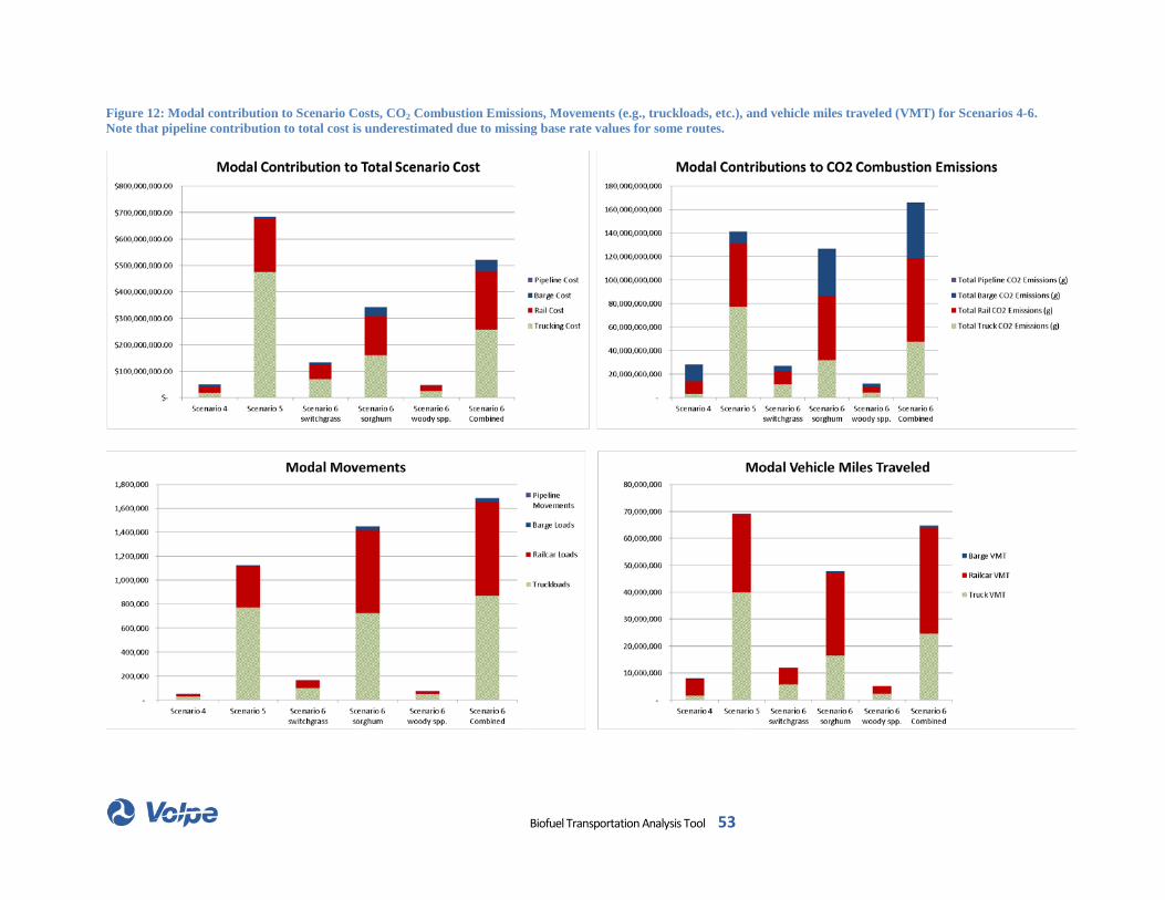
Figure 12: Modal contribution to Scenario Costs, CO2 Combustion Emissions, Movements (e.g., truckloads, etc.), and vehicle miles traveled (VMT) for Scenarios 4-6. Note that pipeline contribution to total cost is underestimated due to missing base rate values for some routes.
Biofuel Transportation Analysis Tool 53

Figure 13: Per gallon cost of transport for fuel delivered in Scenarios 4-6. Note that pipeline contribution to per unit transport cost is underestimated due to missing base rate values for some routes.
Figure 14: Average CO2 emissions per gallon of fuel delivered in Scenarios 4-6.
Biofuel Transportation Analysis Tool 54
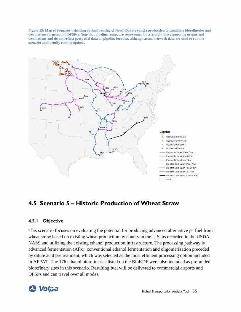
Figure 15: Map of Scenario 4 showing optimal routing of North Dakota canola production to candidate biorefineries and destinations (arports and DFSPs). Note that pipeline routes are represented by a straight line connecting origins and destinations and do not reflect geospatial data on pipeline location, although actual network data are used to run the scenario and identify routing options.
4.5 Scenario 5 – Historic Production of Wheat Straw
4.5.1 Objective
This scenario focuses on evaluating the potential for producing advanced alternative jet fuel from wheat straw based on existing wheat production by county in the U.S. as recorded in the USDA NASS and utilizing the existing ethanol production infrastructure. The processing pathway is advanced fermentation (AFx): conventional ethanol fermentation and oligomerization preceded by dilute acid pretreatment, which was selected as the most efficient processing option included in AFPAT. The 176 ethanol biorefineries listed on the BioKDF were also included as prefunded biorefinery sites in this scenario. Resulting fuel will be delivered to commercial airports and DFSPs and can travel over all modes.
Biofuel Transportation Analysis Tool 55

4.5.2 Geographical Scope
This scenario is national in scope, constrained only by selection of counties where wheat straw production meets a minimum threshold level of 35,000 metric tons of feedstock production. For this scenario it is assumed that 100% of the available wheat straw is available for conversion. The 176 existing ethanol facilities in the US (as reported by the BioKDF database) were also included in the analysis.
4.5.3 Key Parameter Values
The wheat straw data are derived from wheat production in the U.S. in 2012 as recorded in the USDA NASS. This scenario includes a minimum biorefinery capacity of 30 million gallons per year and a maximum of 200 million gallons per year. The unmet demand penalty was $2,000 per kgal, the maximum feedstock transport distance was set at 250 miles, and the minimum county-level feedstock production amount was 35,000 metric tons.
4.5.4 Run Summary
AFTOT processed Scenario 5 in approximately eighteen hours. There were 379 preprocessors with sufficient production to meet the minimum threshold, and 132 potential destinations were included resulting in 44,000 OD pairs. Three hundred twenty five candidate biorefinery locations were generated, of which 76 were deleted because of IDW ranking, leaving 249 candidate sites for the optimization. Of these, 68 were used in the optimal solution. Potential feedstock production was nearly 45 million metric tons. This amount of feedstock could hypothetically result in total potential fuel production (diesel, jet, naptha, etc.) of 1.5 billion gallons of fuel. In this scenario, jet fuel demand was 8.6 billion gallons per year and diesel was 1.1 billion gallons per year.
4.5.5 Results/Conclusions
In Scenario 5, 36 million metric tons, or about 79% of the total available feedstock was used in the optimal solution. Conversion of this feedstock produced 900 million gallons of jet fuel and 224 million gallons of diesel in the 68 biorefineries selected for the optimal solution. The fuel was delivered to 41 different airports (see Table 9). In aggregate, the fuel delivered met about 10% of the jet fuel demand and about 20% of the diesel demand designated in the scenario.
Biofuel Transportation Analysis Tool 56

Table 11: Destinations receiving jet and/or diesel fuel and percent demand fulfilled at airports and DFSPs in Scenario 5. Note that airport codes and names are listed in Appendix A – Airports Abbreviations.
Destination (DFSP name or airport code)
% Jet Demand % Diesel Demand
ABQ 100 100 AMA 100 100 AUS 0 6 BNA 3 100 BOI 0 100 BUR 15 34 CLE 0 100 CMH 0 100 Columbus, GA DFSP 100 0 COS 100 100 DAL 0 100 DEN 100 100 DFW 34 100 DSM 100 100 DTW 3 100 GEG 100 100 ICT 100 100 IND 2 100 Indianapolis, IN DFSP 100 0 LCK 0 100 LIT 72 100 MCI 100 100 MDW 28 100 MEM 4 10 MKE 0 100 MSP 100 100 MSY 0 10 Novi_MI DFSP 99 0 OKC 100 100 Olathe KS DFSP 100 0 Omaha, NE DFSP 100 0 ORD 28 100 Pasco, WA DFSP 100 0 PDX 100 100 SDF 6 55 SEA 10 78 Selby, CA DFSP 2 0 SMF 0 8 STL 100 100 TUL 100 100
Biofuel Transportation Analysis Tool 57

Destination (DFSP name or airport code)
% Jet Demand % Diesel Demand
TUS 9 100 Vancouver, WA DFSP 100 0 All Destinations 10 20
This solution included use of all the surface modes of transportation, including 773,000 truckloads traveling 40 million vehicle miles, as well as 350,000 rail cars traveling 29 million rail car miles. 660 bargeloads covered 78,000 vehicle miles. And nearly 10,000 miles of pipeline were used for 79 movements. However, trucking and rail dominated the transport cost in this scenario. Figure 13 presents graphical descriptions of contributions of the different modes toward total scenario cost, CO2 emissions, movements, and vehicle miles traveled. Figure 15 shows the results of this scenario. One can see the concentration of feedstock production in the central and upper Midwest, represented by the clusters of green feedstock production points. The feedstock from these facilities is delivered to biorefineries by truck and rail, then moved by all modes from biorefineries to airports and DFSPs across a large portion of the country, although the central West and Northeast did not receive alternative fuel delivery from this scenario.
The total cost to move this material was $685 million of which approximately $474.5 million was trucking cost, $202 million was rail cost, $6.7 million was barging cost, and $1.3 million was pipeline cost. This resulted in a per gallon fuel transport cost of approximately $0.61 per gallon, which is higher than in the other scenarios.
Biofuel Transportation Analysis Tool 58

Figure 16: Map of Scenario 5 showing a national wheat straw scenario based on historical wheat production patterns, advanced fermentation processing, delivery to airports and DFSPs,, and transporting via all modes. Note that pipeline routes are represented by a straight line connecting origins and destinations and do not reflect actual geospatial data on pipeline location, although actual network data are used to run the scenario and identify routing options.
4.6 Scenario 6 – Billion Ton Feedstock Production Scenario
4.6.1 Objective
This scenario is actually a combination of three distinct scenarios run for different feedstocks and processes based on the Billion Ton Study data. This scenario focuses on evaluating the downstream transportation, processing, and distribution patterns of alternative jet fuel generated from feedstocks identified in the U.S. Department of Energy (DOE) Billion Ton Study Update (Perlack and Stokes 2011). The study was intended to estimate potential biomass available within the contiguous United States and includes assumptions about production capacity and technology availability, and provides supply curves (i.e., price vs. feedstock availability). It attempts to use conservative assumptions so as not to over-estimate availability. It includes county-by-county estimates of potential availability of specific feedstocks that can be used in
Biofuel Transportation Analysis Tool 59

AFTOT as origin points. For the AFTOT scenario, the baseline Billion Ton Study data were used for the 2018 year and $80/dry ton price point. Feedstocks are processed based on the most efficient processing option for each feedstock type as identified in AFPAT. Fuels are delivered to U.S. commercial airports and DFSPs.
4.6.2 Geographical Scope
This scenario is national in scope and counties are selected based on meeting a minimum production threshold of 10,000 metric tons of feedstock.
4.6.3 Key Parameter Values
For switchgrass, the processing pathway was via advanced fermentation (AFx), with a minimum biorefinery capacity of 30 million gallons per year and a maximum of 200 million gallons per year. For sweet sorghum, the most efficient process identified in AFPAT was Fischer-Tropsch (FTx) processing, with a minimum biorefinery capacity of 100 million gallons per year and maxium of 200 million gallons per year, as FT facilities tend to be larger. For hardwood species, the most efficient processing type was pyrolysis (PRx), with a minimum biorefinery capacity of 10 million gallons per year and a maximum of 200 million gallons per year. The unmet demand penalties for the three feedstocks (switchgrass, sorghum, hardwoods) were $2,000, $4,000, and $2,000, respectively, to better match the varying capital costs associated with the different processes. The maximum feedstock transport distances were 250, 150 and 250 respectively, and the minimum preprocessor production amounts were 50,000, 35,000, and 50,000 metric tons, respectively – the sorghum scenario had lower material availability and therefore needed a lower threshold origin size to identify an optimal scenario.
4.6.4 Run Summary
Total combined run time for these three feedstocks was approximately 13 hours. There were 325 preprocessors above the minimum production floor (78, 211, and 36 for switchgrass, sorghum, and hardwoods, respectively) and 132 final destinations with a total jet fuel demand of 8.65 billion gallons per year and total diesel demand of 1.1 billion gallons. Nearly 42,000 OD pairs were processed during the analysis. The total potential feedstock production was 810 million metric tons, which had the potential to be converted into 50 billion gallons of fuels, with a total potential for 552 supported biorefineries (12 AFx, 491 FT and 49 PRx facilities). AFTOT generated 325 total biorefinery candidate locations and deleted 102 because of IDW (1, 66, and 35 , respectively). Two hundred and twenty-three biorefinery locations were used in the optimal solution ( 187, 23, and 13, respectively).
4.6.5 Results/Conclusions
Biofuel Transportation Analysis Tool 60
Based on the optimized scenarios for each feedstock/process combination, the total amount of feedstock used was 94 million metric tons, or about 12% of total available feedstock (78, 11, and 88% of switchgrass, sorghum, and woody feedstock used, respectively). This resulted in production of 1.5 billion gallons of jet fuel and 1.4 billion gallons of diesel, fulfilling 17% and 121% of demand, respectively. Due to the high diesel production from these scenarios, low diesel demand at the airports, and the single pathway run constraint, this combination of scenarios delivers excess diesel to some destinations. This highlights the need for the user to adjust scenario demand values when running multiple feedstock/pathway scenarios to the same destinations. Future development will include an approach to address the issue either by enabling aggregated demand limitations or by integrating multiple conversion processes into a single optimization scenario. Table 8 shows the airports and DFSPs that received fuel in this scenario and the amounts provided from each sub-scenario, as well as the total demand fulfillment.
Biofuel Transportation Analysis Tool 61

Table 12: Destinations receiving jet and/or diesel fuel and percent demand fulfilled at airports and DFSPs for Scenario 6. Note that airport codes and names are listed in Appendix A – Airports Abbreviations.
Scenario 6 Switchgrass Scenario 6 Sorghum Scenario 6 Woody Spp. Scenario 6 Combined
Destination % Jet Demand Filled
% Diesel Demand Filled
% Jet Demand Filled
% Diesel Demand Filled
% Jet Demand Filled
% Diesel Demand Filled
Total % Jet Fulfilled
Total % Diesel Fulfilled
ABQ
100 100
100 100 Alamogordo, NM DFSP
100 100
100 100
ALB
100 100 0 100 100 200 AMA 0 97 100 100
100 197
Annacostia DFSP
100 100
100 100 ATL 0 1 0 100
0 101
AUS
100 100
100 100 Baltimore, MD DFSP
100 100
100 100
BDL
100 100
100 100 BNA
0 100 0 64 0 164
BOI
0 100
0 100 BOS
0 100
0 100
Bremen, GA DFSP 31 0
31 0
BUF 0 72 0 100 0 100 0 272 BUR
0 100
0 100
BWI
4 100 0 100 4 200 Charleston, SC DFSP 100 0
100 0
CHS 66 100 0 100
66 200 CLE 91 100 0 100 0 100 91 300 CLT 14 31 63 100
77 131
Biofuel Transportation Analysis Tool 62

Scenario 6 Switchgrass Scenario 6 Sorghum Scenario 6 Woody Spp. Scenario 6 Combined
Destination % Jet Demand Filled
% Diesel Demand Filled
% Jet Demand Filled
% Diesel Demand Filled
% Jet Demand Filled
% Diesel Demand Filled
Total % Jet Fulfilled
Total % Diesel Fulfilled
CMH 100 100 0 100 0 100 100 300 COS
0 100
0 100
Craney Island, VA DFSP 0 1 100 100
100 101
CRP
100 100
100 100 CVG
85 100 0 60 85 160
DAB
0 100
0 100 DAL
100 100
100 100
DCA
100 100 0 100 100 200 DEN
0 100
0 100
DFW
71 100
71 100 DSM 0 85 0 100
0 185
DTW 12 69 0 100 0 100 12 269 Ells Jet, SD DFSP
100 100
100 100
ELM
0 100 0 100 0 200 ELP
0 100
0 100
EWR
0 100 0 41 0 141 FLL
0 100
0 100
GEG
0 100
0 100 GRR
0 100 0 100 0 200
GSP
100 100
100 100 Holy Corp , ID DFSP
100 100
100 100
HOU
0 100
0 100 Houston, TX DFSP
65 100
65 100
HPN
0 100
0 100 HRL
100 100
100 100
Biofuel Transportation Analysis Tool 63

Scenario 6 Switchgrass Scenario 6 Sorghum Scenario 6 Woody Spp. Scenario 6 Combined
Destination % Jet Demand Filled
% Diesel Demand Filled
% Jet Demand Filled
% Diesel Demand Filled
% Jet Demand Filled
% Diesel Demand Filled
Total % Jet Fulfilled
Total % Diesel Fulfilled
IAD
0 100
0 100 IAH
0 100
0 100
ICT 63 100 100 100
163 200 IND
0 100 0 100 0 200
ISP
0 100
0 100 ITH 100 100 0 100 0 100 100 300 Jacksonville, FL DFSP
0 100
0 100
JFK
0 100 0 28 0 128 LAS
11 100
11 100
LAX
0 100
0 100 LCK 100 100 0 100 0 100 100 300 LGA
24 100 0 100 24 200
LGB
0 100
0 100 LIT
100 100
100 100
Ludlow, MA DFSP
100 100
100 100
Mayport, FL DFSP 0 56 0 100
0 156
MCI 0 39 100 100
100 139 MCO
0 100
0 100
MDW
0 100 0 100 0 200 MEM 2 5 0 100
2 105
MHT
0 100
0 100 MIA
0 100
0 100
MKE
100 100 0 100 100 200 MSP 7 25 40 100 0 100 46 225 MSY
0 100
0 100
Biofuel Transportation Analysis Tool 64

Scenario 6 Switchgrass Scenario 6 Sorghum Scenario 6 Woody Spp. Scenario 6 Combined
Destination % Jet Demand Filled
% Diesel Demand Filled
% Jet Demand Filled
% Diesel Demand Filled
% Jet Demand Filled
% Diesel Demand Filled
Total % Jet Fulfilled
Total % Diesel Fulfilled
OAK
0 100
0 100 OKC
100 100
100 100
Olathe, KS DFSP 65 0 100 100
165 100 Omaha, NE DFSP 100 0 100 100
200 100
ONT
0 100
0 100 ORD
8 100 0 100 8 200
ORF 0 100 100 100
100 200 PBI
0 100
0 100
PDX
0 100
0 100 PHL
23 100 0 23 23 123
PHX
0 100
0 100 PIT
0 100 0 100 0 200
PNS
0 100
0 100 Point Loma, CA DFSP
0 100
0 100
Port Mahon, DE DFSP
100 100
100 100
Puget Sound, WA DFSP
0 100
0 100
PVD
0 100
0 100 RDU 0 100 0 100
0 200
RNO
0 100
0 100 ROC 100 100 0 100 0 100 100 300 RSW
0 100
0 100
SAN
0 100
0 100 SAT
0 100
0 100
SDF
0 100
0 100 SEA
0 100
0 100
Biofuel Transportation Analysis Tool 65

Scenario 6 Switchgrass Scenario 6 Sorghum Scenario 6 Woody Spp. Scenario 6 Combined
Destination % Jet Demand Filled
% Diesel Demand Filled
% Jet Demand Filled
% Diesel Demand Filled
% Jet Demand Filled
% Diesel Demand Filled
Total % Jet Fulfilled
Total % Diesel Fulfilled
Selma_ 68 0 0 0
68 0 SFB
0 100
0 100
SFO
0 100
0 100 SJC
0 100
0 100
SLC
85 100
85 100 SMF
0 100
0 100
SNA
0 100
0 100 SRQ
0 100
0 100
STL
0 100
0 100 TPA
0 100
0 100
TUL
100 100
100 100 TUS
100 100
100 100
Watson, CA DFSP
0 100
0 100
Yorktown, VA DFSP
100 100
100 100
All Destinations 2 4 15 100 0 17 17 121
Biofuel Transportation Analysis Tool 66

Figure 16 shows the outcomes of each of the feedstock/pathway scenarios that were combined for Scenario 6 total results. Many different airports and DFSPs were supplied with alternative jet fuel by these three scenarios. The sorghum/FT pathway analysis covered the broadest geographical area. The total transport cost of the scenario was $523 million, of which $257 million was for trucking (25 million VMT 5y about 870,000 truckloads), $222 million for rail transport (40 million VMT by about 786,000 rail cars), $40.7 million was for barge transport (approximately 783,000 VMT by 26,000 bargeloads), and $2.6 million was for pipeline movement (68 movements), with the caveat that the pipeline movement costs are underestimated due to missing base rates for some routes. Figure 13 presents graphical descriptions of contributions of the different modes toward total scenario cost, CO2 emissions, movements, and vehicle miles traveled. Average per gallon fuel transport cost also varied widely, ranging from $0.58/gal) for switchgrass-derived AFx fuels to 0.14/gal for sorghum-derived FT Fuels to $0.25/gal for hardwood-based PRx fuels. The average per unit cost of fuel transport was $0.18/gal..
Total CO2 emissions associated with all of these movements was 166,300 metric tons, of which about 70,000 metric tons caome from rail, 48,000 from trucking, and 47,000 from barge transport.
Biofuel Transportation Analysis Tool 67

Figure 17: Map of Scenario 6 showing a national analysis of multiple feedstocks as identified in the Billion Ton Study Update by the U.S. DOE, delivery to airports and DFSPs,, and transporting via all modes. Feedstocks included a) switchgrass processed by advanced fermentation, b) sweet sorghum processed by Fischer-Tropsch, and c) hardwood species processed by pyrolysis. Note that pipeline routes are represented by a straight line connecting origins and destinations and do not reflect actual geospatial data on pipeline location, although actual network data are used to run the scenario and identify routing options.
Biofuel Transportation Analysis Tool 68

5 Conclusion This report summarizes the development and current capabilities of the AFTOT model, which is an expansion of the former “BTAT” model. AFTOT includes the capability to effectively optimize transport for multiple feedstocks and fuels at regional and national scales based on transportation-specific costs and weightings, feedstock processing information, conversion process efficiency, product slate, and capital cost, and other user-defined parameters. The tool now includes waterway transport by barge as well as a partial pipeline network, and these have been successfully integrated into the AFTOT optimization process. This version of AFTOT also includes the capability to address seasonality of harvest and movements by incorporating explicit time-steps into the model. The ability to take in yield and process information from the AFPAT tool has also been expanded.
The test scenarios included herein demonstrate these capabilities at multiple scales and provide insight into particular future scenarios of alternative fuel production. The more realistic scenarios (Scenarios 4-6) are based on existing feedstock production data and demand centers, for which AFTOT provides screening level analysis to understand potential for cost-effective delivery of feedstocks and fuels throughout the continental U.S.
Scenario 4 using USDA breakeven data for canola shows that even from a narrow production zone (North Dakota), airports and DFSPs around the country may be supplied with alternative jet fuel when using optimal transportation patterns to move feedstock and fuel along the transportation network. The wheat straw results (Scenario 5) corroborate this result, showing delivery from the central US to many places in the east, southeast, and southwest. The Billion Ton Study scenarios together cover most of the US and suggested that transport to over 100 airports and DFSPs could be achieved from these feedstock scenarios based on optimized transport patterns and costs. Management of demand over multiple scenarios will need to be addressed in a future phase of development to better enable fulfillment of demand without over-delivery of materials when multiple conversion process are being modeled.
The scenarios presented herein demonstrate the capabilities of the current AFTOT version. AFTOT provides a foundation for testing a variety of assumptions about how future scenarios will affect transportation patterns and what the associated cost and emissions implications of those patterns will be. Future expansions will build on this fundamental basis for expanded fuels scenario testing.
Biofuel Transportation Analysis Tool 69

6 Recommendations for Development of Turn-key Biofuel Feedstock and Fuel Transportation Modeling Tool
6.1 Next Steps
An additional phase of development has already been funded by FAA. Phase 3 of AFTOT development will include:
1) Completion of pipeline integration
The current version of AFTOT includes 10 complete and 20 partial pipeline systems. In Phase 3, the remaining pipeline systems will be added and the origin-destination pairs will be completed for all systems.
2) Additional scenarios
The current version of the tool, plus the remaining pipeline network elements, will be used to run additional scenarios, potentially including ASCENT Project 1, CAAFI State Initiatives, Farm 2 Fly 2.0 analyses, parallel runs with ORNL to compare their models to AFTOT, etc.
3) Petroleum processing infrastructure To better understand the available infrastructure for alternative fuel production (e.g., for co-processing and/or blending), GIS layers for petroleum blenders and refineries will be added to the network
4) Existing roadway flows To begin to develop capabilities to investigate capacity issues, existing flows on the network must be taken into account. To start with, Phase 3 will include incorporation of roadway flows from FAF into a network layer that can be overlain onto the AFTOT intermodal network.
Biofuel Transportation Analysis Tool 70

6.2 Future Needs - Additional Future Tasks Necessary to Create a Turnkey Model
The longer term opportunity to turn AFTOT into a user-friendly, easily accessible tool would require the implementation of more functions within the tool itself, as well as specific user interface capabilities to allow a novice user without extensive GIS experience to work with the tool and test scenarios. Additional future tasks that might be required to create a turnkey version of AFTOT that could be easily disseminated to a wide user audience include:
• Create user interface to enable novice user to run system and enter inputs • Develop user interface for regional capacity screening • Excision of restricted datasets with option to incorporate user datesets in their place • Code modifications to enable deployment • Greater automation of features to enable user modification • Create self-contained installation package
Other potential expansions could include
• Addition of Hawaii, Canada, or other non-CONUS locations. • Incorporation of existing flows on railway, waterway and barge • Incorporation of commodity-specific existing flow data (e.g., existing agricultural
commodities, petroleum products) • Incorporation of gas and oil fields as sources of fossil-based fuels for combined modeling • Development of FAF-level and regional-level capacity analysis for roadways • Development of capacity analysis capability for rail • Add option to calculate life cycle CO2 equivalent emissions • Allocate feedstock transport costs and GHG emissions in accordance with accepted life
cycle methodologies. • Incorporate future capacity/infrastructure plans/projections • Address system resilience/reliability – e.g., identify locations where excess capacity
could allow for system redundancy, identify biorefinery or destination supplies that are vulnerable to disruption from single route disruptions.
• Add option of requiring movement of a minimum volume of fuels (for example, for a volumetric regulatory requirement such as the Renewable Fuel Standard) to drive the scenario.
The development of a capacity analysis capability for the different modes would enable evaluation of whether scenarios would exceed the capacity of available infrastructure. The following section outlines some considerations for developing such an approach.
Biofuel Transportation Analysis Tool 71

6.3 AFTOT and Transportation Capacity
The capacity of a transportation link is limited by both the availability of vehicles and of line capacity. For example, a railroad origin-destination movement for a commodity may be limited by both the availability of cars of the correct type, as well as the capacity of the rail line to handle trains between two points. Similar constraints apply for other modes.
Congestion occurs when the demand for transportation reaches or exceeds the vehicle or line capacity. Two types of congestion issues are relevant to the scenarios run in AFTOT:
First is where the added feedstock and fuel flows become a significant portion of the total flow on a transportation network element (e.g, a rail line), and create a congestion problem. This is most likely to occur in the vicinity of large preprocessors and biorefineries. It may also occur near destinations if the AFTOT flow arrives by a different mode of transportation than what was previously used for fossil fuel flow.
Second is where AFTOT flows are added to links that are already congested. The AFTOT flow may add marginally to the congestion, and it may be worthwhile to choose AFTOT routings that avoid these areas.
6.3.1 Symptoms of a Capacity Issue
A capacity issue will manifest itself in several ways:
First is via pricing. If prices can be set freely, the transportation provider can increase the price charged so that demand is reduced to available supply. So, an unusually high price for a particular movement may indicate a capacity issue.
Second is via availability of transportation. For example, there may be a long wait for rail cars of a certain type.
Third is via increased travel time and reduced travel time reliability. As a link on the transportation network (highway, rail or water) becomes more congested, travel times increase, and may become less reliable, because small changes in demand or capacity (e.g., a closed lane) can have larger effects on travel time as demand approaches capacity.
6.3.2 Challenges in Addressing Capacity
Biofuel Transportation Analysis Tool 72

There are several significant challenges in addressing capacity. First is understanding exactly what the capacity is. If the issue is availability of vehicles (rail cars or trucks), this information is generally privately held. Furthermore, the capacity in terms of vehicle availability will often depend on the direction of flow. In the primary flow direction (head haul), capacity may be tightly constrained, as all of the vehicles are full. However, in the other direction (back haul), there may be significant available capacity, as most of the vehicles are moving empty. With vehicles that are more specialized (e.g., a tanker truck versus a box trailer), these head haul / back haul differences are likely to be more pronounced.
If the capacity issue is one of link capacity (e.g., vehicles per hour on a highway), some resources are available.
An older report that provides some quick rules-of-thumb on highway link capacity is NCRHP Report 365: Travel Estimation Techniques for Urban Planning (Martin and McGuckin 1998)Chapter 10 provides some useful approximations. More detailed capacity estimation for highways and road intersections can be found in the Highway Capacity Manual (Transportation Research Board 2010). Typically, highway capacity is a function of the type of road (is it a freeway or local road?), the number and type of intersections (are there signals or stop signs?) and the number of lanes.
For rail capacity, some information is available in the National Rail Freight Infrastructure Capacity and Investment Study(Cambridge Systematics 2007), which as commissioned by the Association of American Railroads. This report noted that “capacity of rail corridors is determined by a large number of factors, including the number of tracks, the frequency and length of sidings, the capacity of the yards and terminals along a corridor to receive the traffic, the type of control systems, the terrain, the mix of train types, the power of the locomotives, track speed, and individual railroad operating practices. “ Factors used in their analysis included tracks, type of control (signal) systems, and mix of train types.
The second major challenge in addressing capacity is that in order to understand congestion, and where capacity issues might exist, it is necessary to know about the background traffic volumes on a link and how they compare to the capacity of a link, in addition to the AFTOT generated volumes. This information may not be readily available.
Furthermore, capacity is highly time dependent. Most highways are not congested 24 hours / day, and capacity issues on other modes may be highly seasonal. Finally, since AFTOT is a planning model of flows that may be several years in the future, today’s capacity issues may not be the same as tomorrow’s. Background traffic might grow, or, conversely, a highway might be expanded.
6.3.3 How to Address Capacity
Biofuel Transportation Analysis Tool 73

There are three approaches to addressing capacity, presented below in increasing order of difficulty in modeling.
1. First is to run an uncapacitated model, and simply report the volumes on transportation linksand well as the numbers of vehicles used. This is what is done now, and provides usefulinformation as to where alternative fuel movements are likely to significantly contribute tocapacity issues. It does not require knowledge of background traffic volumes or linkcapacities.
2. To reducing the AFTOT-recommended volume on a link because of known capacity issues,one could block flow over the link entirely, or add an artificial cost to the link that would behigh enough to reduce optimal flow volume over that link.
3. The final step would be an explicit modeling of capacity. This requires a complete picture ofthe background volume on the link, as well as its capacity. This level of modeling may bemost appropriate when performing detailed modeling of the area near a biorefinery ordestination, where the AFTOT-flows on the transportation links are a significant proportionof the total flows.
Biofuel Transportation Analysis Tool 74
Biofuel Transportation Analysis Tool 75
7 References Airlines For America. 2012. A4A Quarterly Cost Index: U.S. Passenger
Airlines: http://www.airlines.org/Pages/A4A-Quarterly-Cost-Index-U.S.-Passenger-Airlines.aspx. Argonne National Laboratory. 2014. GREET 2014 - available at: https://greet.es.anl.gov/greet/index.htm.
Argonne National Laboratory. Bureau of Transportation Statistics. 2011. National Transportation Atlas Database. Available
at: http://www.rita.dot.gov/bts/sites/rita.dot.gov.bts/files/publications/national_transportation_atlas_database/2011/index.html.
Cambridge Systematics. 2007. National Rail Freight Infrastructure Capacity and Investment Study. EPA. 2012. MOVES (Motor Vehicle Emission Simulator) 2010b. Available
at: http://www.epa.gov/otaq/models/moves/#generalinfo. EPA Office of Transportation and Air Quality.
ESRI. undated. How inverse distance weighted interpolation works. Available at: http://help.arcgis.com/En/Arcgisdesktop/10.0/Help/index.html#//00310000002m000000.
Federal Aviation Administration. 2011. FAA Destination 2025. Washington, DC. Federal Highway Administration. 2013. Freight Analysis Framework (FAF) version 3.4. Lewis, K. C., G. M. Baker, T. T. Lin, S. Smith, O. Gillham, A. Fine, S. Costa, Z. Chen, and C. Cooper. 2014.
Biofuel Transportation Analysis Tool: Description, Methodology, and Demonstration Scenarios - available at: http://ntl.bts.gov/lib/51000/51100/51114/DOT-VNTSC-FAA-14-02.pdf. Cambridge, MA.
Martin, W., and N. McGuckin. 1998. NCHRP Report 365: Travel Estimation Techniques for Urban Planning. Transportation Research Board, Washington, DC.
McDuffie, W. 2013. Teleconference discussion of fuel transport costs. Volpe National Transportation Systems Center.
Perlack, R. D., and B. J. Stokes. 2011. U.S. Billion-Ton Update: Biomass Supply for a Bioenergy and Bioproducts Industry. ORNL/TM-2011/224. Oak Ridge National Laboratory, U.S. Department of Energy, Oak Ridge, TN.
Shepard, D. 1968. A two-dimensional interpolation function for irregularly-spaced data. Proceedings - 1968 ACM National Conference.
Surface Transportation Board. 2011. Carload Waybill Sample. Transportation Research Board. 2010. Highway Capacity Manual. USDA. 2007. 2007 Agricultural Census Data, available at: http://quickstats.nass.usda.gov/. USDA
National Agricultural Statistics Service. USDA Agricultural Marketing Service. 2014. RE: DOT/Volpe Follow-up: AFTOT Project & Transport Cost
Data Needs (email communication from USDA AMS Team (Adam Sparger et al.) to AFTOT team r.e. data request.in S. Costa and K. C. Lewis, editors.

Appendix A – AFTOT Airports List and Abbreviations
Airports included in AFTOT Destinations Layer Abbreviation Full Name State ANC Ted Stevens Anchorage International Airport AK JNU Juneau International Airport AK PHX Phoenix Sky Harbor International Airport AZ TUS Tucson International Airport AZ BUR Bob Hope Airport CA LAX Los Angeles International Airport CA OAK Oakland International Airport CA ONT Ontario International Airport CA SAN San Diego International Airport CA SFO San Francisco International Airport CA SJC Norman Y. Mineta San José International Airport CA SMF Sacramento International Airport CA SNA John Wayne Airport – Orange County CA COS City of Colorado Springs Municipal Airport CO DEN Denver International Airport CO BDL Bradley International Airport CT ECP Northwest Florida Beaches International Airport FL FLL Fort Lauderdale–Hollywood International Airport FL MCO Orlando International Airport FL MIA Miami International Airport FL PBI Palm Beach International Airport FL RSW Southwest Florida International Airport FL SFB Orlando Sanford International Airport FL SRQ Sarasota–Bradenton International Airport FL TPA Tampa International Airport FL ATL Hartsfield-Jackson Atlanta International Airport GA HNL Honolulu International Airport HI ITO Hilo International Airport HI KOA Kona International Airport at Keahole HI LIH Lihue Airport HI OGG Kahului Airport HI MDW Chicago Midway International Airport IL ORD Chicago O'Hare International Airport IL IND Indianapolis International Airport IN
Alternative Fuel Transportation Optimization Tool 76

Airports included in AFTOT Destinations Layer
Abbreviation Full Name State DSM Des Moines International Airport IO CVG Cincinnati/Northern Kentucky International Airport KY MSY Louis Armstrong New Orleans International Airport LA BOS General Edward Lawrence Logan International Airport MA BWI Baltimore/Washington International Thurgood Marshall
Airport MD
DTW Detroit Metropolitan Wayne County Airport MI MSP Minneapolis–St. Paul International Airport MN MCI Kansas City International Airport MO STL Lambert-St. Louis International Airport MO CLT Charlotte/Douglas International Airport NC RDU Raleigh-Durham International Airport NC EWR Newark Liberty International Airport NJ ABQ Albuquerque International Sunport NM LAS McCarran International Airport NV RNO Reno/Tahoe International Airport NV BUF Buffalo Niagara International Airport NY JFK John F. Kennedy Intenational Airport NY LGA LaGuardia Airport NY ROC Greater Rochester International Airport NY CLE Cleveland-Hopkins International Airport OH CMH Port Columbus International Airport OH LCK Rickenbacker International Airport OH OKC Will Rogers World Airport OK TUL Tulsa International Airport OK PDX Portland International Airport OR PHL Philadelphia International Airport PA PIT Pittsburgh International Airport PA PVD Theodore Francis Green State Airport RI CHS Charleston International Airport SC BNA Nashville International Airport TN MEM Memphis International Airport TN AFW Fort Worth Alliance Airport TX AUS Austin-Bergstrom International Airport TX DAL Dallas Love Field TX DFW Dallas/Fort Worth International Airport TX ELP El Paso International Airport TX HOU William P. Hobby Airport TX IAH George Bush Intercontinental Airport TX SAT San Antonio International Airport TX SLC Salt Lake City International Airport UT DCA Ronald Reagan Washington National Airport VA
Alternative Fuel Transportation Optimization Tool 77
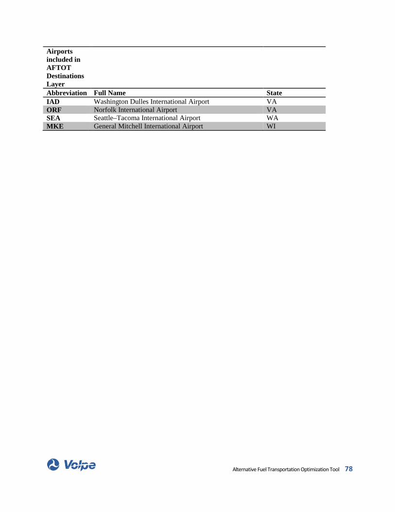
Airports included in AFTOT Destinations Layer
Abbreviation Full Name State IAD Washington Dulles International Airport VA ORF Norfolk International Airport VA SEA Seattle–Tacoma International Airport WA MKE General Mitchell International Airport WI
Alternative Fuel Transportation Optimization Tool 78

Appendix B – AFTOT Default DFSP List
LOCATION Abbreviation in AFTOT DFSP Alamogordo, NM Alamogo DFSP Annacostia, DC Annacos DFSP Baltimore, MD Baltimo DFSP Boston, MA Boston DFSP Bremen, GA Bremen DFSP Carson, CA Carson DFSP Charleston, SC Charles DFSP Columbus PL, GA Columbu DFSP Craney Island, VA Craney_ DFSP Ells Jet, SD Ells_Je DFSP Holy Corp, ID Holy_Co DFSP Houston, TX Houston DFSP Indianapolis, IN Indiana DFSP Jacksonville, FL Jack_FL DFSP Jacksonville, NJ Jack_NJ DFSP Key West Pipeline, FL Key_Wes DFSP Lebanon, OH Lebanon DFSP Lockhart Pipeline, MS Lockhar DFSP Ludlow, MA Ludlow DFSP Macon, GA Macon_ DFSP Mayport, FL Mayport DFSP Montgomery, AL Montgom DFSP Moundville, AL Moundvi DFSP New Haven, CT New_Hav DFSP Novi, MI Novi_M DFSP Olathe, KS Olathe DFSP Omaha, NE Omaha_ DFSP Pasco, WA Pasco_ DFSP Pittsburg, PA Pittsbu DFSP Point Loma, CA Point_L DFSP Port Everglades, FL Port_Ev DFSP Port Mahon, DE Port_Ma DFSP Portland, ME Portlan DFSP Puget Sound, WA Puget_S
Alternative Fuel Transportation Optimization Tool 79

LOCATION Abbreviation in AFTOT DFSP Selby, CA Selby_ DFSP Selma, NC Selma_ DFSP Standard Transpipe, VA Standar DFSP Tampa, FL Tampa_ DFSP Vancouver, WA Vancouv DFSP Watson, CA Watson DFSP Yorktown, VA Yorktow
Alternative Fuel Transportation Optimization Tool 80

Appendix C – XML-based Scenario Input File Example This sample input file shows the variables that can be modified by a user of the analytical tool, with sample inputs from Scenario 1.
Alternative Fuel Transportation Optimization Tool 81
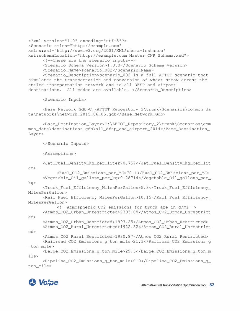
<?xml version="1.0" encoding="utf-8"?> <Scenario xmlns="http://example.com" xmlns:xsi="http://www.w3.org/2001/XMLSchema-instance" xsi:schemaLocation="http://example.com Master_ONR_Schema.xsd"> <!--These are the scenario inputs--> <Scenario_Schema_Version>1.3.0</Scenario_Schema_Version> <Scenario_Name>scenario_002</Scenario_Name> <Scenario_Description>scenario_002 is a full AFTOT scenario that simulates the transportation and conversion of wheat straw across the entire transportation network and to all DFSP and airport destinations. All modes are available. </Scenario_Description> <Scenario_Inputs> <Base_Network_Gdb>C:\AFTOT_Repository_2\trunk\Scenarios\common_data\networks\network_2015_06_05.gdb</Base_Network_Gdb> <Base_Destination_Layer>C:\AFTOT_Repository_2\trunk\Scenarios\common_data\destinations.gdb\all_dfsp_and_airport_2014</Base_Destination_Layer> </Scenario_Inputs> <Assumptions> <Jet_Fuel_Density_kg_per_liter>0.757</Jet_Fuel_Density_kg_per_liter> <Fuel_CO2_Emissions_per_MJ>70.4</Fuel_CO2_Emissions_per_MJ> <Vegetable_Oil_gallons_per_kg>0.28714</Vegetable_Oil_gallons_per_kg> <Truck_Fuel_Efficiency_MilesPerGallon>5.8</Truck_Fuel_Efficiency_MilesPerGallon> <Rail_Fuel_Efficiency_MilesPerGallon>10.15</Rail_Fuel_Efficiency_MilesPerGallon> <!--Atmospheric CO2 emissions for truck are in g/mi--> <Atmos_CO2_Urban_Unrestricted>2393.08</Atmos_CO2_Urban_Unrestricted> <Atmos_CO2_Urban_Restricted>1993.25</Atmos_CO2_Urban_Restricted> <Atmos_CO2_Rural_Unrestricted>1922.52</Atmos_CO2_Rural_Unrestricted> <Atmos_CO2_Rural_Restricted>1930.87</Atmos_CO2_Rural_Restricted> <Railroad_CO2_Emissions_g_ton_mile>21.3</Railroad_CO2_Emissions_g_ton_mile> <Barge_CO2_Emissions_g_ton_mile>29.5</Barge_CO2_Emissions_g_ton_mile> <Pipeline_CO2_Emissions_g_ton_mile>0.0</Pipeline_CO2_Emissions_g_ton_mile>
Alternative Fuel Transportation Optimization Tool 82

</Assumptions> <!--These are the input parameters to run all of the scripts.--> <scriptParameters> <!--Updates the network with the cost functions defined by the user. CREATE NETWORK SCRIPT --> <Create_Network_Layer_Script> <Network_Costs> <Intermodal_Costs_Per_Gallon_Mile> <Railroad> <!--Railroad_Class_I_Cost is in dollars per thousand gallon-mile--> <Railroad_Class_I_Cost>0.12</Railroad_Class_I_Cost> </Railroad> <Truck> <!--Truck_Base_Cost is in dollars per thousand gallon-mile--> <Truck_Base_Cost>0.45</Truck_Base_Cost> <!--Truck_Interstate includes FAF Function Classes 1,11,12--> <Truck_Interstate_Weight>1.00</Truck_Interstate_Weight> <!--Truck_Principal_Arterial includes FAF Function Classes 2,14--> <Truck_Principal_Arterial_Weight>1.10</Truck_Principal_Arterial_Weight> <!--Truck_Minor_Arterial includes FAF Function Classes 6,16--> <Truck_Minor_Arterial_Weight>1.20</Truck_Minor_Arterial_Weight> <!--Truck_Local includes all other FAF Functions Classes (excluding those above)--> <Truck_Local_Weight>1.30</Truck_Local_Weight> </Truck> <Barge> <!--Barge_Cost is in dollars per thousand gallon-mile--> <Barge_cost>0.05</Barge_cost> </Barge> <Pipeline> <!--Pipeline_cost is found from a table of Tarrifs based on origin-destination pair--> <Pipeline_cost>0.01</Pipeline_cost> </Pipeline> </Intermodal_Costs_Per_Gallon_Mile> <Intermodal_Transloading_Costs> <transloading_dollars_per_ton>40.00</transloading_dollars_per_ton> <!-- NOT CURRENTLY USED -->
Alternative Fuel Transportation Optimization Tool 83

<transloading_dollars_per_thousand_gallons>40.00</transloading_dollars_per_thousand_gallons> </Intermodal_Transloading_Costs> </Network_Costs> </Create_Network_Layer_Script> <!--Calculate the preprocessor locations and fuel production. This assumes that a county shapefile with the crop yield data has already been created. CREATE PREPROCESSOR LOCATIONS SCRIPT --> <Create_Preprocessor_Location_Script> <Feedstocks_to_Use> <Feedstock> <Base_Feedstock_Gdb>C:\AFTOT_Repository_2\trunk\Scenarios\common_data\preprocessors.gdb</Base_Feedstock_Gdb> <!--Available Feedstocks: Corn Stover, Wheat Straw, Canola, Harwood - General, Softwood - General, Switchgrass, Sweet sorghum, Sugarcane Bagasse, Corn, Camelina, Jatropha, Salicornia, Edible Tallow, Inedible Tallow, Lard, Poultry Fat, Yellow Grease, Other Greases, Harwood - American Sycamore, Harwood - Black Locust, Harwood - Eastern Cottonwood, Harwood - Eucalyptus, Harwood - Hybrid Poplar, Harwood - Yellow Poplar, Softwood - Monterey Pine, Softwood - General, Big Bluestem, Sericea Lespedeza, Switchgrass, Tall Fescue, Agave, Sweet sorghum, Forage sorghum--> <Feedstock_type>Wheat Straw</Feedstock_type> <!--Available Feedstock Sources: NASS, FBEP, USDA--> <Feedstock_Data_source>NASS</Feedstock_Data_source> <!--Available Feedstock Units: Tonne, Metric Ton, Short Ton, Long Ton, Weight Ton, Pound, Gross Ton, Cubic Meter, US Gallon, US Quart, US Pint--> <Feedstock_unit>AFPAT</Feedstock_unit> <!--N/A, kg/m3, kg/L--> <Feedstock_density_unit>N/A</Feedstock_density_unit> <Feedstock_density>0</Feedstock_density> <Replacement_Percentage>100</Replacement_Percentage> <!--Time periods are weekly, 52 weeks in a year, minimum Time_Period_Start = 1, maximum Time_Period_End = 52--> <Time_Period_Start>1</Time_Period_Start> <!--Time periods are weekly, 52 weeks in a year, minimum Time_Period_Start = 1, maximum Time_Period_End = 52--> <Time_Period_End>1</Time_Period_End> <!--Available Primary Processing Types: AFx, SRx (n-paraffins), SRx (n-/iso-paraffins), CRx, PRx, FTx, HEFA--> <Primary_Processing_Type>AFx</Primary_Processing_Type>
Alternative Fuel Transportation Optimization Tool 84

<!--Dilute acid pretreatment, Dilute alkali pretreatment, Aq. Ammonia pretreatment, Conventional milling technology, Advanced milling technology (low GHG), Advanced milling technology (high GHG), N/A--> <Secondary_Processing_Type>Dilute acid pretreatment</Secondary_Processing_Type> <!--Available Tertiary_Processing_Types: Advanced fermentation to alkanes (low GHG), Advanced fermentation to alkanes (mid GHG), Advanced fermentation to alkanes (high GHG), Advanced fermentation to fatty acids (low GHG), Advanced fermentation to fatty acids (mid GHG), Advanced fermentation to fatty acids (high GHG), Advanced fermentation to TAGs (low GHG), Advanced fermentation to TAGs (mid GHG), Advanced fermentation to TAGs (high GHG), Conventional fermentation to ethanol (low GHG), Conventional fermentation to ethanol (mid GHG), Conventional fermentation to ethanol (high GHG), Conventional fermentation to butanol (low GHG), Conventional fermentation to butanol (mid GHG), Conventional fermentation to butanol (high GHG)--> <Tertiary_Processing_Type>Conventional fermentation to ethanol (mid GHG)</Tertiary_Processing_Type> </Feedstock> </Feedstocks_to_Use> <!--Minimum production floor is metric tons per time period per country/preprocessor. --> <Minimum_Production_Floor>35000</Minimum_Production_Floor> </Create_Preprocessor_Location_Script> <!--Create a shapefile with the biorefinery candidate locations. This step requires that the user create the network dataset in ArcCatalog. Right click on the geodatabase, select New, Feature Dataset. Right click on the feature dataset, select New, Network Dataset. Follow the wizard prompts to create the Network Dataset. The cost basis is named "cost_" + the scenario name, e.g., if the scenario name is called "subset", the cost basis is "cost_subset". You will need to update this XML file with the correct path to the Network Dataset. The tag is at the top in the "Scenario_Inputs" section. CREATE BIOREFINERY CANDIDATES SCRIPT --> <Create_Biorefinery_Candidates_Script> <Maximum_Raw_Material_Travel_Distance_Miles>250</Maximum_Raw_Material_Travel_Distance_Miles> <!--Enter 'AFPAT' if these values should be derived from AFPAT--> <Min_Biorefinery_Capacity_Kgal>30000</Min_Biorefinery_Capacity_Kgal>
Alternative Fuel Transportation Optimization Tool 85

<Max_Biorefinery_Capacity_Kgal>200000</Max_Biorefinery_Capacity_Kgal> <Biorefinery_Building_Fixed_Cost_Dollars>6000000</Biorefinery_Building_Fixed_Cost_Dollars> <Currently_Funded_Biorefineries> <Biorefinery> <Name>Null</Name> <Latitude>Null</Latitude> <Longitude>Null</Longitude> <Capacity_Gallons>Null</Capacity_Gallons> </Biorefinery> </Currently_Funded_Biorefineries> <!-- and/or specify a layer --> <Currently_Funded_Biorefineries_Layer>C:\AFTOT_Repository_2\trunk\Scenarios\common_data\biorefineries.gdb\BioenergyKDF_EthanolRefineries</Currently_Funded_Biorefineries_Layer> </Create_Biorefinery_Candidates_Script> <!--inputNetworkDataset as first input, costLayer is networkLayer, costField is cost_to_use, origins_fc is preproc, ROUTE OPTIMIZATION SCRIPT --> <Route_Optimization_Script> <Max_Artificial_Link_Distance_Miles>5</Max_Artificial_Link_Distance_Miles> <Penalty_For_Not_Fulfilling_Depot_Demand>2000</Penalty_For_Not_Fulfilling_Depot_Demand> </Route_Optimization_Script> <!--Data reporting DATA REPORTING SCRIPT --> <Data_Reports_Script> </Data_Reports_Script> </scriptParameters> </Scenario>
Alternative Fuel Transportation Optimization Tool 86