Alireza Mousavi

Brunel University

1

» 2nd order systems

» General characterisation of 2nd TF

» Stability of System

» Routh-Hurwitz Stability Criterion

2

» The differential equation of a 2nd order system:

𝑎2𝑑2𝑦

𝑑𝑡2+ 𝑎1

𝑑𝑦

𝑑𝑡+ 𝑎0𝑦 = 𝑏0𝑢 (1)

The Laplace transform of a simple 2nd order system with IC=0:

𝐺 𝑠 =𝑌(𝑠)

𝑈(𝑠)=

𝑏0

𝑎2𝑠2+𝑎1𝑠+𝑎0

(2)

» Consider:

G 𝑠 =6

𝑠2 + 5𝑠 + 6

Apply a unit step 𝐻 𝑡 =1

𝑢(𝑡)⇒ 𝑈 𝑠 =

1

𝑠

Therefore;

𝑌 𝑠 = 𝐺 𝑠 𝑈 𝑠 ⇒6

𝑠 𝑠2 + 5𝑠 + 6=

6

𝑠(𝑠 + 2)(𝑠 + 3)

3

Expanding the X(s) into partial fractions:

𝑌 𝑠 =1

𝑠−

3

𝑠 + 2+

2

𝑠 + 3

From the standard table of Laplace Transforms:

𝑦 𝑡 = 1 − 3𝑒−2𝑡 + 2𝑒−3𝑡 𝐻(𝑡)

The unit step:

4

0 0.5 1 1.5 2 2.5 30

0.5

1

y(t)

t

» Consider a system with TF: 𝐺 𝑠 =10

𝑠2+2𝑠+5

» Apply a unit step input:

So 𝑦 𝑡 = 2 − 2𝑒−𝑡𝑐𝑜𝑠2𝑡 − 𝑒−𝑡𝑠𝑖𝑛2𝑡 𝐻(𝑡)

It can be converted into: 𝑦 𝑡 = 2 − 𝐴𝑒−𝑡sin(2𝑡 + 𝜑)

Where: 𝐴 = 22 + 12 = 5

And 𝜑 = 𝑡𝑎𝑛−1 21 = 1.11𝑟𝑎𝑑[63.4°]

5

Y s 10

s s2 2s 5

2

s

2s 4

s2 2s 5

Y s 2

s

2 s 1 2

s 1 2 5 1

2

s

2 s 1 s 1

2 22

2

s 1 2 22

The unit step response will look like:

6

0 1 2 3 4 50

1

2

y(t)

t

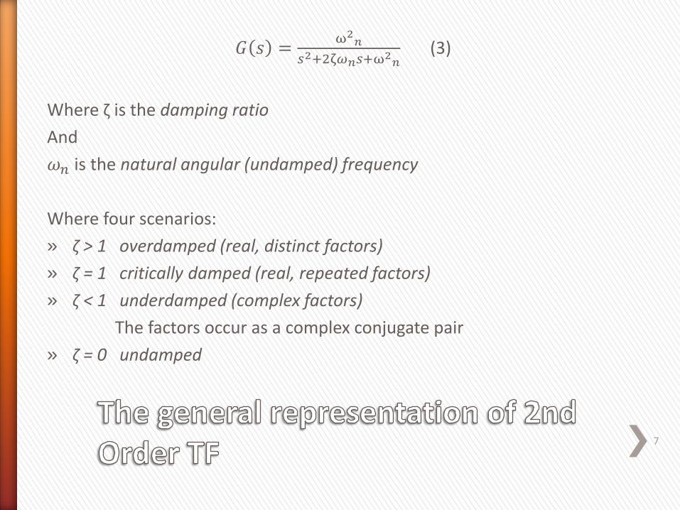
𝐺 𝑠 =ω2

𝑛

𝑠2+2ζ𝜔𝑛𝑠+ω2𝑛 (3)

Where ζ is the damping ratio

And

𝜔𝑛 is the natural angular (undamped) frequency

Where four scenarios:

» ζ > 1 overdamped (real, distinct factors)

» ζ = 1 critically damped (real, repeated factors)

» ζ < 1 underdamped (complex factors)

The factors occur as a complex conjugate pair

» ζ = 0 undamped

7

For the underdamped case (0 < ζ <1), the unit step response with zero IC would be:

(4)

For different ζ values the unit step response would look like:

The frequency of

oscillation is:

𝜔𝑑 = 𝜔𝑛 1 − ζ2

8

𝑦 𝑡 = 1 −1

1−ζ2𝑒−ζ𝜔𝑛𝑡sin(𝜔𝑛𝑡 1 − ζ2 + 𝑐𝑜𝑠−1ζ)

0

0.2

0.4

0.6

0.8

1

1.2

1.4

1.6

1.8

0 1 3 4 5 6 7 8 9 102

nt

y t

0.1

0.25

0.5

0.7

1

It helps to characterise the 2nd order step response as:

Where:

𝑡𝑟 is the rise time

𝑡𝑝is the first peak

PO is the % overshoot

𝑡𝑠 is the setting time for the response to fall within a prescribed band round about the final steady state value

9

0 t

y t

tr

tp

ts

% overshoot ( PO )

100

𝑡𝑝 can be found by differentiating y(t) and setting the derivative equal to zero.

The time for the first peak is: 𝑡𝑝 =𝜋

𝜔𝑛 1−ζ2

Alternatively, note that the transient response oscillates at the damped

natural frequency, 𝜔𝑑 = 𝜔𝑛 1 − ζ2

Time to first peak = ½ of the period = 1

2×

2𝜋

𝜔𝑑=

𝜋

𝜔𝑑

At this point the output will be: 𝑦 𝑡𝑝 = 1 + 𝑒𝑥𝑝−𝜋ζ

1−ζ2

∴ 𝑃𝑂 = 𝑒𝑥𝑝−𝜋ζ

1 − ζ2× 100%

10

11

0

20

40

60

80

100

0 0.1 0.2 0.3 0.4 0.5 0.6 0.7 0.8 0.9 1

Percentage Overshoot vs Damping Ratio

Damping ratio,

% O

ve

rsh

oo

t, PO

𝑡𝑟 is found by setting y(t) = 1 an solving the lowest value of t

Giving 𝜔𝑛 1 − ζ2𝑡𝑟 + 𝑐𝑜𝑠−1ζ = 𝜋

∴ 𝑡𝑟 =𝜋−𝑐𝑜𝑠−1ζ

𝜔𝑛 1−ζ2

𝑡𝑠 is found by the amplitude term 𝑒−ζ𝜔𝑛𝑡 in y(t) (see equation 4 slide 8)

» this is a decaying exponential term with time constant of 1

ζ𝜔𝑛

The response would decay within 5% of the final value after 3 times constants or 2% of the final value after 4 times constants etc.

So for settling to within 5%, 𝑡𝑠 = 3

ζ𝜔𝑛 and 2%, 𝑡𝑠 =

4

ζ𝜔𝑛

12

» A system can be categorised as stable if it is excited by an input, it has transients which dissipate in time and leave the system in its steady-state condition.

» A system can be considered as unstable if the transients do not die off with time but increase in size, thus the steady-state is never reached.

» Consider an input of a unit of impulse to a first order system with:

𝐺 𝑠 =1

𝑠+1 the system output Y(s):

𝑌 𝑠 = 𝐺 𝑠 𝑈 𝑠 =1

𝑠 + 1× 1

and thus the 𝑦 = 𝑒−𝑡 as time t increases the output dies away equal to zero.

Stable System

Now if the transfer function is: 𝐺 𝑠 =1

𝑠−1, 𝑌 𝑠 =

1

𝑠−1× 1.

Therefore, 𝑦 = 𝑒𝑡 , as t increases output increases, ever increasing output. Thus the system is Instable.

13

» Remember that the values of s that make the TF infinite are the Poles.

» In other words the roots of characteristic equation.

In the case of 𝐺 𝑠 =1

𝑠−1, s = 1 and 𝐺 𝑠 =

1

𝑠+1 , s = -1 are the poles.

unstable (s positive) stable (s negative)

14

y

t

y

t

» For 2nd order system with TF:

𝐺 𝑠 =ω2

𝑛

𝑠2 + 2ζ𝜔𝑛𝑠 + ω2𝑛

When subject to a unit of impulse input:

𝑌 𝑠 =ω2

𝑛

(𝑠 + 𝑝1)(𝑠 + 𝑝2)

Where 𝑝1 and 𝑝2 are the roots of equation:

𝑠2 + 2ζ𝜔𝑛𝑠 + 𝜔𝑛 = 0

Using the equation for roots of quadratic equation:

𝑝 =−2ζ𝜔𝑛 ± 4ζ2ω2

𝑛 − 4ω2𝑛

2= −ζ𝜔𝑛 ± 𝜔𝑛 ζ2 − 1

15

» Depending on the value of ζ (damping factor), the term under the square root can be real or imaginary.

» In case there is an imaginary term the output involves an oscillation.

Let’s look at 2 scenarios

16

1. 𝐺 𝑠 =𝐾

𝑠2+11𝑠+10=

𝐾

(𝑠+1)(𝑠+10) two real poles : stable

System mode will persist much longer due to pole at s = -1 than the system mode due to pole at s = -10.

No zero to influence the magnitude of the modes.

Therefore pole at s = -1 will dominate transient response of system

17

-10 -1

j

s - plane

t t

real parts

Imaginary parts

2. 𝐺 𝑠 =𝐾

𝑠2+2𝑠+5=

𝐾

(𝑠+1+2𝑗)(𝑠+1−2𝑗) two complex conjugate poles

𝑠2 + 2ζ𝜔𝑛𝑠 + ω2𝑛 𝜔𝑛 = 5; ζ=

1

5

𝑠 = −ζ𝜔𝑛 ± 𝑗𝜔𝑛 1 − ζ2 stable system

18

j

s - plane

-1

+2j

-2j

r

t

𝜔𝑛 = 𝑟 = 22 + 12 = 5

ζ = 𝑐𝑜𝑠𝜃 =1

5

confirm from the characteristic polynomial

The frequency of oscillation, 𝜔𝑑 in the output response

- given by the imaginary component of the poles (𝜔𝑑 = 2𝑟𝑎𝑑𝑠−1 in this case)

- Conforming that 𝜔𝑑 = 𝜔𝑛 1 − ζ2

19

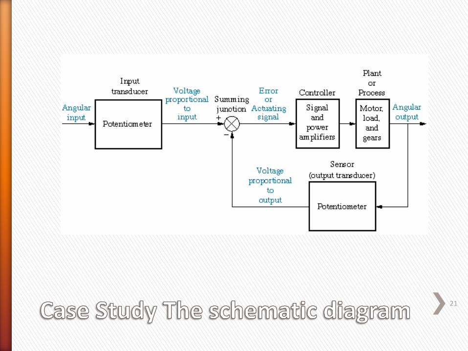
Antenna Azimuth Position Control System

The diagram of the system:

20

21

» Consider a system described by a 1st order LDE:

𝑑𝑦

𝑑𝑡+ 𝑎𝑦(𝑡) = 𝑏𝑢(𝑡)

Adopting the Laplace transforms:

𝑠𝑌 𝑠 − 𝑦 0 + 𝑎𝑌 𝑠 = 𝑏𝑈 𝑠 ⇒ 𝑌 𝑠 =1

𝑠 + 𝑎𝑦 0 +

𝑏

𝑠 + 𝑎𝑈(𝑠)

For stability, we consider the zero input response 𝑦0 𝑡 :

𝑦0 𝑡 = 𝑦(0)𝑒−𝑎𝑡𝐻(𝑡)

If 𝑎 > 0 then the system is stable (the exponential term decays)

If 𝑎 < 0then the system is unstable (the exponential term increases)

If 𝑎 = 0 the exponential term become 1, therefore the response is constant the system is marginally stable

22

Generally;

» a system is asymptotically stable if 𝑦0(𝑡) → 0 as 𝑡 → ∞

i.e. the output response due to initial energy in the system decays to zero as t becomes large.

» a system is marginally stable if for each set of initial conditions there is a finite positive constant M such that:

𝑦0(𝑡) ≤ 𝑀 for all 𝑡 ≥ 0

{in general, M depends on the initial conditions}

i.e. the output response is bounded in magnitude.

» a system is unstable if there are values of the initial conditions for which

𝑦0(𝑡) → ∞ as 𝑡 → ∞

i.e. the output response grows without bound for some values of initial conditions.

23

For higher order systems:

» the free response is determined by the modes of the systems: 𝑦0 𝑡 = 𝐶1𝑒

−𝑝1𝑡 + 𝐶2𝑒−𝑝2𝑡 + ⋯+ 𝐶𝑛𝑒

𝑝𝑛𝑡

where are the system poles (real or complex)

if a pole is real, the exponential term decays if the pole is negative.

» for complex conjugate poles; 𝑠 = ζ𝜔𝑛 ± 𝑗𝜔𝑛 1 − ζ2

The response is oscillatory with an exponential term 𝑒ζ𝜔𝑛𝑡

˃ if ζ > 0 (real part of the pole is negative), exponential term decays ⇒ system is stable

˃ if ζ < 0 (real part of the pole is positive), exponential term grows unbounded ⇒ system is unstable

˃ if ζ = 0 exponential term = 1 ⇒system is marginally stable - constant oscillations

24

All higher order systems consist of combinations of the above terms

» if just a single exponential term grows unbounded ⇒ system is unstable

Stability Theorem:

A system is stable if and only if all system poles lie in the left half of the s-plane.

25

» The Routh-Hurwitz stability criterion is simple way to determine whether a system is stable or not (i.e. whether non of the poles have positive real parts).

» It is achieved by examining the characteristic of polynomial without solving the characteristic equation for its roots.

» If the system is unstable the Routh-Hurwitz test will tell us the number of poles that are on the right half of the s-plane

» First step is to establish the Routh array.

26

The Characteristic Equation (CE) can be expressed as: 𝑎𝑛𝑠

𝑛 + 𝑎𝑛−1𝑠𝑛−1 + 𝑎𝑛−2𝑠

𝑛−2 + ⋯+ 𝑎0 = 0

» In order for the system to be stable, all the roots must lie on the left half of the s-plane.

» The necessary condition for stability is that all the coefficients are present and have the same sign.

» Sufficient conditions are obtained from the following table:

27

𝒔𝒏 𝒂𝒏 𝒂𝒏−𝟐 𝒂𝒏−𝟒 … 1st row

𝒔𝒏−𝟏 𝒂𝒏−𝟏 𝒂𝒏−𝟑 𝒂𝒏−𝟓 … 2nd row

𝒔𝒏−𝟐 𝒃𝟏 𝒃𝟐 𝒃𝟑 … 3rd row

𝒔𝒏−𝟑 𝒄𝟏 𝒄𝟐 𝒄𝟑 … 4th row

… . . . …

𝒔𝟎 𝒉𝟏 Last row

» The first two rows are completed using the 𝑎𝑛, 𝑎𝑛−1, … , 𝑎1, 𝑎0 (coefficients)of the characteristic polynomial.

» Note the alternate coefficients in these two first rows. i.e. first row 𝑎𝑛, 𝑎𝑛−2, … and second row 𝑎𝑛−1, 𝑎𝑛−3, …

» Each subsequent row is calculated from elements of the two immediately above rows, by cross-multiplying the elements of the two rows:

𝑏1 =𝑎𝑛−1𝑎𝑛−2−𝑎𝑛𝑎𝑛−3

𝑎𝑛−1,

𝑏2 =𝑎𝑛−1𝑎𝑛−4−𝑎𝑛𝑎𝑛−5

𝑎𝑛−1, or 𝑏𝑛−𝑘 = −

1

𝑎𝑛−1

𝑎𝑛 𝑎𝑛−𝑘

𝑎𝑛−1 𝑎(2𝑘+1)

𝑐1 =𝑏1𝑎𝑛−3−𝑎𝑛−1𝑏2

𝑏1,

𝑐2 =𝑏1𝑎𝑛−5−𝑎𝑛−1𝑏3

𝑏1, or 𝑐𝑛−𝑘= −

1

𝑏𝑛−1

𝑎𝑛−1 𝑎𝑛−(2𝑘+1)

𝑏𝑛−1 𝑏𝑛−(𝑘+1)

And so on …

28

Just to recap again, conditions for stability based on Routh-Hurwitz Criterion:

1. All the coefficients (𝑎𝑛, 𝑎𝑛−1, … , 𝑎𝑛) of the characteristic equation should be of same sign (positive or negative).

2. All the elements of the first column of the Routh array must be positive or the same sign.

3. If the system is unstable, the number of unstable poles is given by the number of successive sign changes in the elements of the first column of the Routh array.

29

Example 1: Consider a closed-loop system with transfer function to be:

𝐺 𝑠 =1

(𝑠3−𝑠2+2𝑠+1)

Without creating the Routh array we can see that the system is unstable since condition 1 is not met. Because the coefficients of the CE are not of same sign.

30

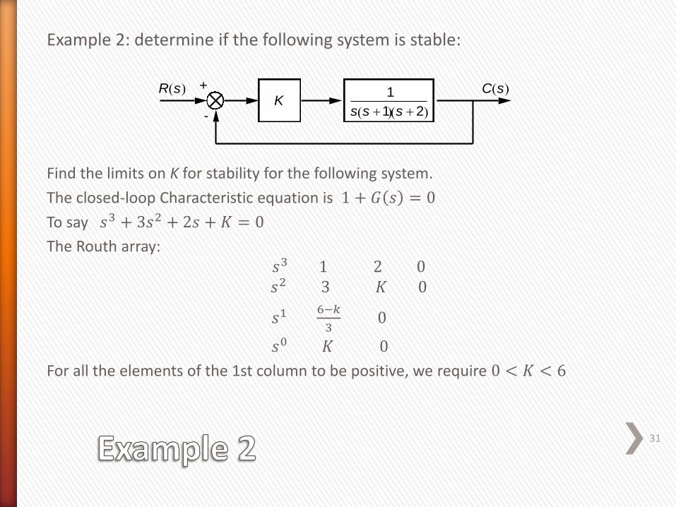
Example 2: determine if the following system is stable:

Find the limits on K for stability for the following system.

The closed-loop Characteristic equation is 1 + 𝐺 𝑠 = 0

To say 𝑠3 + 3𝑠2 + 2𝑠 + 𝐾 = 0

The Routh array: 𝑠3120 𝑠23𝐾0

𝑠1 6−𝑘

30

𝑠0𝐾0

For all the elements of the 1st column to be positive, we require 0 < 𝐾 < 6

31

+

-

R s C s K

1

s s 1 s 2

» Note: at either extreme value, the Routh array has a zero row - for this example this represents roots on the imaginary axis.

» These roots can be found from the auxiliary equation formulated from the elements in the row that precedes the row of zeros.

» For example K = 6 the elements of 𝑠1 row are zero. The auxiliary equation is:

3𝑠2 + 6 = 0 which gives the roots 𝑠 = ±𝑗 2.

32