algorithms for multiphase partitioning
TRANSCRIPT

Algorithms for Multiphase Partitioning
by
Matthew Jacobs
A dissertation submitted in partial fulfillmentof the requirements for the degree of
Doctor of Philosophy(Mathematics)
in the University of Michigan2017
Doctoral Committee:
Professor Selim Esedoglu, Co-ChairProfessor Jinho Baik, Co-ChairAssociate Professor Jason CorsoProfessor Peter Miller


For my parents.
ii

ACKNOWLEDGMENTS
This thesis would not be possible without the contributions of manywonderful people. My friends and family, who patiently supportedduring my time in Michigan. My friend, Olivia Walch, who got meinterested in the whole business of programming and computer vision.My collaborators, Pengbo Zhang and Ekaterina Merkurjev, who madecollaborative research a joy. My advisor, Jinho Baik, who mentored andsupported me over many years. I am especially thankful to my advisorand collaborator, Selim Esedoglu, for his mentorship, his insights andfor accepting me as his student as I neared the end of the Ph.D. program.Finally, I am grateful for support from the National Science Foundationduring part of this thesis work.
iii

TABLE OF CONTENTS
Dedication . . . . . . . . . . . . . . . . . . . . . . . . . . . . . . . . . . . . . . . ii
Acknowledgments . . . . . . . . . . . . . . . . . . . . . . . . . . . . . . . . . . . iii
List of Figures . . . . . . . . . . . . . . . . . . . . . . . . . . . . . . . . . . . . . vi
List of Tables . . . . . . . . . . . . . . . . . . . . . . . . . . . . . . . . . . . . . . viii
List of Abbreviations . . . . . . . . . . . . . . . . . . . . . . . . . . . . . . . . . ix
Abstract . . . . . . . . . . . . . . . . . . . . . . . . . . . . . . . . . . . . . . . . . x
Chapters
1 Introduction . . . . . . . . . . . . . . . . . . . . . . . . . . . . . . . . . . . . . 1
1.1 Background and Previous Work . . . . . . . . . . . . . . . . . . . . . . 31.1.1 Threshold dynamics . . . . . . . . . . . . . . . . . . . . . . . . 71.1.2 The heat content energy . . . . . . . . . . . . . . . . . . . . . . 8
1.2 Summary of Contributions . . . . . . . . . . . . . . . . . . . . . . . . . 12
2 Convolution Kernels and Stability of Threshold Dynamics Methods . . . . . . 14
2.1 Introduction . . . . . . . . . . . . . . . . . . . . . . . . . . . . . . . . . 142.2 New Variants of Threshold Dynamics . . . . . . . . . . . . . . . . . . . 15
2.2.1 Non-monotone energy and oscillating solutions . . . . . . . . . . 152.2.2 A new variant: Single growth . . . . . . . . . . . . . . . . . . . 162.2.3 Multiphase Single Growth Algorithm . . . . . . . . . . . . . . . 23
2.3 Convergence of non-local energies . . . . . . . . . . . . . . . . . . . . . 292.4 Conclusions . . . . . . . . . . . . . . . . . . . . . . . . . . . . . . . . . 38
3 Kernels with Prescribed Surface Tension and Mobility for Threshold Dynam-ics Schemes . . . . . . . . . . . . . . . . . . . . . . . . . . . . . . . . . . . . . 39
3.1 Introduction . . . . . . . . . . . . . . . . . . . . . . . . . . . . . . . . . 393.2 Preliminaries and Notation . . . . . . . . . . . . . . . . . . . . . . . . . 393.3 Previous Work . . . . . . . . . . . . . . . . . . . . . . . . . . . . . . . . 413.4 The New Convolution Kernels . . . . . . . . . . . . . . . . . . . . . . . 44
3.4.1 Positive Kernels . . . . . . . . . . . . . . . . . . . . . . . . . . 443.4.2 Kernels with Positive Fourier Transform . . . . . . . . . . . . . . 53
3.5 Numerical Evidence . . . . . . . . . . . . . . . . . . . . . . . . . . . . . 56
iv

3.5.1 Two-phase, anisotropic flows . . . . . . . . . . . . . . . . . . . . 573.5.2 Multi-phase, anisotropic flows . . . . . . . . . . . . . . . . . . . 59
3.6 Conclusions . . . . . . . . . . . . . . . . . . . . . . . . . . . . . . . . . 63
4 Auction Dynamics:A Volume Preserving MBO Scheme . . . . . . . . . . . . . . . . . . . . . . . . 65
4.1 Auction Dynamics . . . . . . . . . . . . . . . . . . . . . . . . . . . . . 654.1.1 The assignment problem . . . . . . . . . . . . . . . . . . . . . . 664.1.2 Auction algorithms . . . . . . . . . . . . . . . . . . . . . . . . . 694.1.3 Upper and lower volume bounds . . . . . . . . . . . . . . . . . . 744.1.4 Auction dynamics with temperature . . . . . . . . . . . . . . . . 82
4.2 Curvature motion . . . . . . . . . . . . . . . . . . . . . . . . . . . . . . 83
5 Semi-Supervised Learning . . . . . . . . . . . . . . . . . . . . . . . . . . . . . 90
5.1 Introduction . . . . . . . . . . . . . . . . . . . . . . . . . . . . . . . . . 905.2 Background and Notation . . . . . . . . . . . . . . . . . . . . . . . . . . 91
5.2.1 The graphical model . . . . . . . . . . . . . . . . . . . . . . . . 915.2.2 Semi-supervised data classification . . . . . . . . . . . . . . . . 92
5.3 Graph MBO Schemes . . . . . . . . . . . . . . . . . . . . . . . . . . . . 935.3.1 MBO via linearizations of GHC . . . . . . . . . . . . . . . . . . 945.3.2 A fidelity term based on graph geodesics . . . . . . . . . . . . . 975.3.3 Schemes with volume constraints and temperature . . . . . . . . 98
5.4 Experimental Results . . . . . . . . . . . . . . . . . . . . . . . . . . . . 1005.4.1 Benchmark datasets . . . . . . . . . . . . . . . . . . . . . . . . 1005.4.2 Experimental results using GHCMBO and GHCMBOS . . . . . . 1025.4.3 Experimental results using GHCMBOV . . . . . . . . . . . . . . 103
5.5 Conclusions . . . . . . . . . . . . . . . . . . . . . . . . . . . . . . . . . 106
6 Conclusion . . . . . . . . . . . . . . . . . . . . . . . . . . . . . . . . . . . . . . 108
Bibliography . . . . . . . . . . . . . . . . . . . . . . . . . . . . . . . . . . . . . . 110
v

LIST OF FIGURES
1.1 Some examples of non-zonoidal polytopes [25]. Note that each polytope has at least one facethat is not centrally symmetric. . . . . . . . . . . . . . . . . . . . . . . . . . . . . 11
2.1 One step of the standard algorithm under the action of kernel K1 on the periodic latticeZ/6Z
⊕Z/5Z. The updated configuration has a higher energy than the starting configura-
tion. . . . . . . . . . . . . . . . . . . . . . . . . . . . . . . . . . . . . . . . . 152.2 Behavior of the standard algorithm under the action of kernel K1 on the periodic lattice
Z/6Z⊕
Z/5Z. The algorithm gets trapped in a periodic loop between the two configura-tions above. The configuration on the right has a higher energy . . . . . . . . . . . . . . 16
3.1 Evolution of an initial circle (black) under motion (1.9) with surface tension and mobilitygiven by (3.53), computed using threshold dynamics algorithm, Algorithm 1.1 and the con-volution kernels from Sections 3.4.2 and 3.4.1 (red), compared against benchmark result ob-tained with front tracking (blue). (a) Using the convolution kernel with positive Fourier trans-form of Section 3.4.2. (b) Using the positive convolution kernel of Section 3.4.1. . . . . . . 59
3.2 Evolution of a cube under volume preserving weighted mean curvature flow towards its Wulffshape the octahedron, with surface tension given by the `∞ norm and constant mobility. Thecorresponding kernel was obtained from the construction of Section 3.4.2. Compare with asimilar experiment in [25] that uses a different convolution kernel that has the same surfacetension but different mobility. . . . . . . . . . . . . . . . . . . . . . . . . . . . . . 60
3.3 The kernels (a) K1,2, (b) K1,3, (c) and K2,3 obtained from the construction of Section 3.4.1for the surface tensions and mobilities used in the triple junction example of Figure 3.4. . . . 61
3.4 Evolution of a three-phase configuration with a pair of triple junctions under anisotropic cur-vature flow; each interface has a distinct prescribed surface tension (two of them anisotropic),two have constant mobility, and one has a normal dependent prescribed mobility, as describedin detail in Section 3.5.2. (a) The initial condition. (b) Final configuration computed usingthreshold dynamics Algorithm 2.2 and the positive kernel construction presented in Section3.4.1 (red), compared to the benchmark result computed using front tracking (blue). (c) Thesame evolution computed using two different threshold dynamics algorithms: Algorithm 2.2shown in thin, solid vs. Algorithm 2.3 shown in thick, dashed line. Algorithm 2.2 is faster, butAlgorithm 2.3 has guaranteed unconditional gradient stability for essentially any collection ofN -choose-2 anisotropic surface tension and mobility pairs. . . . . . . . . . . . . . . . . 62
3.5 The Wulff shapes corresponding to the anisotropies used in the triple junction example. Fromleft to right: Wσ1,2 , Wσ1,3 , and Wσ2,3 . . . . . . . . . . . . . . . . . . . . . . . . . . 63
vi

3.6 Evolution of phase i = 1 out of a total of 27 phases, from two different simulations startingfrom the same initial condition. Top row: σi,j(θ, φ) = µi,j(θ, φ) = 1 for all i 6= j. Bottomrow: σi,1(θ, φ) = 1.1
√1 + 0.3 cos2 φ and µi,1(θ, φ) = 1
1.1
√1 + 0.3 cos2 φ for i 6= 1, and
σi,j(θ, φ) = µi,j(θ, φ) = 1 for i 6= 1 and j 6∈ i, 1. Many topological changes occur on thesurface of the “grain”, where quadruple points can be seen to collide and split numerous times. 63
4.1 Initial condition: Randomly shifted 8 columns of 8 squares that have identical areas. Periodicboundary conditions. . . . . . . . . . . . . . . . . . . . . . . . . . . . . . . . . . 84
4.2 Initial condition: Randomly shifted 17 rectangles that have identical areas. Periodic boundaryconditions. After a long time, there is still one phase with five and another with seven neighbors. 85
4.3 Initial condition: Voronoi diagram of 160 points taken uniformly at random on [0, 1]2. Peri-odic boundary conditions. Each phase preserves its initial area. . . . . . . . . . . . . . . 86
4.4 One “grain” from a total of 32. Initial condition: Voronoi diagram of 32 points taken uniformlyat random on [0, 1]3. Periodic boundary conditions. Each phase preserves its initial volume. . 87
4.5 At final time, from a couple of other angles, with a few of its neighbors showing. . . . . . . 874.6 The initial and final configurations of the volume preserving flow on a randomly shifted cubic
lattice. Each image shows two of the grains. The final configuration is fixed under the flow,but is not the global minimizer of the surface energy. . . . . . . . . . . . . . . . . . . 88
4.7 Running the flow on the 8 subunit cubic lattice with temperature fluctuations leads to theWeaire-Phelan structure. The Weaire-Phelan structure contains two distinct subunits shown inthe first two images, the truncated hexagonal trapezohedron on the left and the pyritohedronon the right. The bottom image shows how 3 of the subunits fit together. . . . . . . . . . . 89
5.1 Behavior of Algorithm 5.1 under the action of the weights A1 on a two-phase configurationwith no fidelity term. The algorithm gets trapped in a periodic loop between the two configu-rations above. The configuration on the right has a higher energy. . . . . . . . . . . . . . 96
vii

LIST OF TABLES
5.1 Benchmark datasets . . . . . . . . . . . . . . . . . . . . . . . . . . . . . . . 1005.2 Three Moons . . . . . . . . . . . . . . . . . . . . . . . . . . . . . . . . . . . 1025.3 MNIST . . . . . . . . . . . . . . . . . . . . . . . . . . . . . . . . . . . . . . 1025.4 Comparing Fidelity terms on MNIST . . . . . . . . . . . . . . . . . . . . . . 1035.5 Opt-Digits . . . . . . . . . . . . . . . . . . . . . . . . . . . . . . . . . . . . 1035.6 COIL . . . . . . . . . . . . . . . . . . . . . . . . . . . . . . . . . . . . . . . 1035.7 GHCMBOV Timing (in seconds) . . . . . . . . . . . . . . . . . . . . . . . . 1045.8 GHCMBOV MNIST Results . . . . . . . . . . . . . . . . . . . . . . . . . . 1055.9 GHCMBOV Optdigits Results. . . . . . . . . . . . . . . . . . . . . . . . . . 106
viii

LIST OF ABBREVIATIONS
PDE partial differential equation
SSL semi-supervised learning
GHC graph heat content
ix

ABSTRACT
Algorithms for Multiphase Partitioning
by
Matthew Jacobs
Chair: Selim EsedogluGiven a region D and a partition, Σ, of D into a number of distinct phases
Σ = (Σ1, . . . ,ΣN), a perimeter functional measures the area of the interfacial
boundaries ∂Σi ∩ ∂Σj with respect to some measure on the surface normals.
Perimeter functionals are at the heart of many important variational models, such
as Mullins’ model for grain boundary motion and the Mumford-Shah model for
image segmentation. The gradient flow of perimeter functionals is a non-linear
partial differential equation (PDE) known as curvature motion or curvature flow.
Our focus is threshold dynamics, an efficient and elegant algorithm for simulating
curvature flow. Recently, in [27], the authors re-derived and significantly gener-
alized the threshold dynamics algorithm using a variational framework based on
the heat content energy. The main thrust of this work is to further explore, ana-
lyze and extend threshold dynamics through the heat content energy. We use this
framework to derive several new threshold dynamics schemes; namely “single
growth” schemes which promise unconditional stability for virtually any situa-
tion of interest, and “auction” schemes which extend threshold dynamics to vol-
ume preserving curvature flow. Along the way, we answer an important and long
standing question in the threshold dynamics community, and present applications
to problems in machine learning.
x

CHAPTER 1
Introduction
Many important physical phenomena are described by a partitioning of space into distinctregions, often called phases. A prominent example occurs in polycrystalline materials,which includes most metals and ceramics. Each phase of a polycrystalline material is agrain (a single crystal piece) with a particular crystallographic structure. The behavior ofsuch materials is largely determined by the configuration of the grains (their shapes andsizes), called the microstructure of the material. In fact, many of the bulk mechanicalproperties of the material are determined by the microstructure. The mismatch between thecrystallographic orientations of neighboring grains induces an excess internal energy thatis dissipated via reconfiguration of the microstructure. Naturally, the excess internal energyis proportional to the perimeter of the interfacial boundaries where distinct grains meet. Ifany of these materials are in a non-frozen state (e.g. if they are heated), the microstructurewill often evolve by grain boundary motion, which in part acts to reduce the interfacialperimeters. Thus, these materials are intimately connected to minimal partition problems.
Minimal partition problems also arise in image processing and computer vision. Afundamental task in these fields is to partition a data set into some number of prescribeddifferent classes. For example, one may want to segment an image into a number of dis-tinct objects and regions. Here, a single phase in a partition may consist of pixels withhomogenous color values, or small image patches with similar features. Obtaining highquality segmentations is closely tied to solving minimal partition problems. Indeed, objectboundaries in natural images tend to be smooth curves or simple polygons.
Functionals measuring the perimeters of partitions are key to variational models formodeling and solving the above problems and phenomena. These include Mullins’ modelfor grain boundary motion [66], and the Mumford-Shah model for image segmentation[67]. More recently, such variational models and their minimization via gradient descenthave also been applied in the context of machine learning and artificial intelligence (e.g.graph partitioning models for supervised clustering of data [33]).
1

To minimize perimeter functionals, one naturally turns to gradient descent. In the vari-ational setting, gradient descent is formulated as a time evolution PDE known as the Euler-Lagrange equation. The Euler-Lagrange equation for the L2 gradient descent of the perime-ter functional is motion by mean curvature of the interface boundaries. Given a point x inthe interface, motion by mean curvature moves x in the direction normal to the interfacewith velocity proportional to the mean curvature of the interface at x. Thus, concave por-tions of the interface bulge outwards, while convex regions contract inwards.
Motion by mean curvature (also known as mean curvature flow) is a singular, degener-ate, non-linear PDE. Mean curvature flow is best understood in the two phase case, whichentails the evolution of single interface. In this setting, mean curvature flow is regularizingon short time scales. For example, C2 curves and surfaces evolving under the flow instan-taneously become smooth (in fact real analytic). However, the flow eventually developssingularities. Any convex curve or surface shrinks down and collapses to a single point infinite time. In two dimensions this is essentially the full story; Grayson showed that anyclosed embedded curve in two dimensions becomes convex and then collapses to a pointunder curvature flow [40]. In dimensions three and above, much more complexity is possi-ble. In particular, the flows of certain embedded surfaces develop non-trivial singularitiesthat result in topological changes. For example, a dumbbell shaped surface with certainproportions (connect two spheres with a long thin cylinder) will split at the handle into twopieces before collapsing into two separate points.
Understanding how to continue the flow after non-trivial singularities develop is themost challenging aspect of curvature flow. In the two-phase case, the theory of viscositysolutions allows one to define a well-posed notion of a solution past the formation of sin-gularities. However, there is no analogous theory in the multi-phase case. Furthermore, inthe multi-phase case much more complicated topological changes are possible. As a result,simulating curvature flow (especially in the multi-phase case) requires sophisticated nu-merical methods. Indeed, the most straight-forward approach known as front tracking (i.e.explicitly parameterizing the interfaces and moving them with the correct normal speed),entails handling topological changes in painful and heuristic ways.
Fortunately, there has been great success simulating curvature flow with methods thatrepresent the interfaces implicitly. One of the most famous examples is the level-set methodof Osher and Sethian [71]. Implicit methods represent embedded curves and surfaces asthe level sets of a function. One obtains the correct motion by repeatedly solving a shorttime evolution equation on the entire function (or in a thin layer near the relevant levelset) and then locating the new position of the level set. The principal advantage is theeffortless handling of topological changes. Indeed, in the level set method, topological
2

changes require no reparameterizations or “surgeries”. The focus of this work will bethreshold dynamics, a level set method specialized for simulating curvature flow.
Originally proposed by Merriman, Bence, and Osher (MBO) in [63, 62], threshold dy-namics – also known as the MBO algorithm or diffusion generated motion – is a veryefficient algorithm for approximating the motion by mean curvature of an interface. Thealgorithm generates a discrete in time approximation to mean curvature motion by alternat-ing two very simple steps: convolution with a kernel, and pointwise thresholding. Amongits benefits are 1. implicit representation of the interface as in the phase field or level setmethods, allowing for graceful handling of topological changes, 2. unconditional stability(for certain kernels), where the time step size is restricted only by accuracy considerations,and 3. very low per time step cost when implemented on uniform grids.
Recently, Esedoglu and Otto gave a variational interpretation of the MBO scheme basedon the heat content energy [27]. Given a partition, the heat content measures the amount ofheat that escapes from each phase under a short time diffusion generated by a convolutionkernel K. At small time scales, the amount of heat that escapes is proportional to theperimeter of the boundary. Thus, the heat content energy is a non-local approximationto the perimeter functional [1], [64], and thus is naturally connected to curvature flow.Esedoglu and Otto showed that one may recover and generalize the MBO algorithm bysuccessively minimizing linearizations of the heat content. This procedure shows that forcertain kernels, the heat content is dissipated at every step of the MBO algorithm. Thus,the heat content is a Lyapunov functional for the MBO scheme, implying unconditionalstability of the algorithm.
The variational interpretation of threshold dynamics via the heat content energy is atthe heart of this work. The starting point of our investigations is the theory developed in[27] and [25]. We build upon this theory, using the heat content to derive and analyzenew “single growth” variants of threshold dynamics. A natural outgrowth of our schemesare new kernel constructions, which allows us to answer some long standing questionsin the threshold dynamics community. In addition, we derive a new multi-phase volumepreserving MBO algorithm and we discuss and present applications to machine learning,in particular the semi-supervised learning (SSL) problem.
1.1 Background and Previous Work
We now develop some notation, background and previous work that will be relevant for allthat follows. We will be concerned with possibly anisotropic interfacial energies defined onpartitions of a domain D. In Chapters 2-4, D will be the d-dimensional torus, i.e. a cube in
3

Rd with periodic boundary conditions. In Chapter 5, D will be a weighted graph (V ,W ),which is a finite collection of points V along with a symmetric matrix W : V × V → Rdescribing the connection strength between any two points. By a partition of D, we meana prescribed number N of sets Σ1, . . . ,ΣN ⊆ D that satisfy
N⋃i=1
Σi = D and Σi ∩ Σj = (∂Σi) ∩ (∂Σj) for i 6= j (1.1)
When working with two phase partitions we will simplify our notation. We will represent(Σ1,Σ2) as a single phase Σ := Σ1, since we may recover Σ2 by taking the complement.
Let Hs denote the s-dimensional Hausdorff measure on D. Then the perimeter func-tional of a two phase partition Σ is
E(Σ) = Hd−1(∂Σ) =
∫∂Σ
dHd−1(x). (1.2)
and the perimeter functional for a multiphase partition Σ = (Σ1, . . . ,ΣN) is
E(Σ) =N∑i=1
Hd−1(∂Σi) =N∑i=1
∫∂Σi
dHd−1(x) (1.3)
We will primarily be interested in more general surface energies where we allow the perime-ter measure to be anisotropic. This level of generality is essential for material sciencesapplications, where interaction energies may depend on the misorientation angles of twograins and the normal of the grain boundary between them. Anisotropic surface measuresare also useful in computer vision applications, for example if one wants to favor detectingcertain shapes over others.
Given a surface tension σ, a strictly positive, continuous, even function σ : Sd−1 →(0,∞) we consider the more general version of (1.2)
E(Σ, σ) =
∫∂Σ
σ(n(x)) dHd−1(x) (1.4)
where n(x) denotes the outward unit normal to ∂Σ. It will be convenient to assume that thesurface tension σ has been extended to σ : Rd → R+ as
σ(x) = |x|σ(x
|x|
)for x 6= 0 (1.5)
so that it is positively 1-homogeneous. We will assume that σ is then a convex function
4

on Rd; this condition will ensure well-posedness (lower semi-continuity) of the two-phaseenergy (1.4). Note that the above conditions imply that σ is a norm on Rd. Define the unitball (i.e. the Frank diagram) Bσ of σ as
Bσ = x : σ(x) ≤ 1
which is thus a closed, convex, centrally symmetric set. We will further require Bσ tobe smooth and strongly convex; this implies that we stay clear of the crystalline cases(where Bσ is a polytope) except via approximation. In two dimensions, we will also writeσ = σ(θ), where θ is the angle that the unit normal makes with the positive x1-axis. In thatcase, strong convexity of Bσ is equivalent to the condition
σ′′(θ) + σ(θ) > 0.
The Wulff shape Wσ associated with the anisotropy σ is defined as
Wσ =
y : sup
x∈Bσx · y ≤ 1
.
The sets Bσ can in turn be obtained from Wσ by the formula
Bσ =
x : sup
y∈Wσ
x · y ≤ 1
,
exhibiting the well known duality between Bσ and Wσ. Our assumptions on Bσ imply thatWσ is also strongly convex and has smooth boundary.
We will also consider the multiphase extension of energy (1.4) to partitions. Let N ∈N+ denote the number of phases, and define the set of pairs of indices:
IN = (i, j) ∈ 1, . . . , N × 1, . . . , N : i 6= j, (1.6)
which doubly enumerates the set of distinct interfaces ∂Σi ∩ ∂Σj . To each interface weassociate a potentially different surface tension σi,j = σj,i satisfying the same properties asthe two phase surface tension σ above. With these definitions, our multiphase energy is:
E(Σ,σ) =∑
(i,j)∈IN
∫(∂Σi)∩(∂Σj)
σi,j(n(x)) dHd−1(x) (1.7)
where σ = σij(i,j)∈IN denotes the collection of surface tensions. Note that in the multi-phase case, even if the surface tensions are isotropic (i.e. constant functions), energy (1.7)
5

does not simplify to (1.3) – each interface may have a different constant.For d = 2 or 3, we will study approximations for L2 gradient flow of energies (1.4) and
(1.7), which are known as weighted mean curvature flow (of an interface and a network).The normal speed of a given interface with surface tension σ in three dimensions under thisflow is
v⊥(x) = µ(n(x))((∂2s1σ(n(x)) + σ(n(x))
)κ1(x) +
(∂2s2σ(n(x)) + σ(n(x))
)κ2(x)
)(1.8)
where κ1 and κ2 are the two principal curvatures, and ∂si denotes differentiation alongthe great circle on S2 that passes through n(x) and has as its tangent the i-th principalcurvature direction. The function µ : S2 → R+ is known as the mobility factor, whichdetermines the speed of the flow in each normal direction (as with the surface tensions, inthe multiphase case each interface may have a different mobility). In two dimensions, theexpression simplifies to
v⊥(x) = µ(n(x))(σ(n(x)) + σ′′(n(x)))κ(x), (1.9)
where κ(x) is the curvature at x.While materials science literature e.g. [23, 46] appears to allow the mobility factor
µ : Sd−1 → R+ in (1.8) or (1.9) to be any positive function of the normal, a natural andimportant subclass of mobilities are those µ that have a convex one-homogeneous extension(as in (1.5)) to Rd. Indeed, as explained in [7], motion law (1.8) arises as gradient descentfor energy (1.4) with respect to a norm µ : Rd → R on normal vector fields on ∂Σ e.g. viathe well-known discrete-in-time minimizing movements [22] procedure of Almgren, Taylor& Wang [2], and independently, Luckhaus & Sturzenhecker [55]:
Σk+1 = arg minΣ
E(Σ, σ) +
1
δt
∫ΣMΣk
dµ∗
Σk(x) dx
(1.10)
where dµ∗
Σkdenotes the distance function to the interface ∂Σk at the k-th time step, with
respect to the dual norm µ∗ of the norm µ:
µ∗(x) = supy :µ(y)≤1
x · y.
In addition to (1.8), a condition known as the Herring angle condition [44] holds alongtriple junctions: For d = 3, at a junction formed by the meeting of the three phases Σi, Σj ,
6

and Σk , this condition reads
(`× ni,j)σi,j(ni,j) + (`× nj,k)σj,k(nj,k) + (`× nk,i)σk,i(nk,i)
+ nj,iσ′i,j(ni,j) + nk,jσ
′j,k(nj,k) + ni,kσ
′k,i(nk,i) = 0 (1.11)
where ni,j is the unit normal vector to the interface (∂Σi) ∩ (∂Σj) pointing in the Σi to Σj
direction, ` = nj,k×ni,j is a unit vector tangent to the triple junction, and σ′i,j(ni,j) denotesderivative of σi,j taken on S2 in the direction of the vector `× ni,j . In the isotropic setting,(1.11) simplifies to the following more familiar form, known as Young’s law:
σi,jni,j + σj,knj,k + σk,ink,i = 0. (1.12)
Finally, we note that well-posedness (lower semi-continuity) of the multiphase energy(1.7) in its full generality is a complicated matter [3]. At the very least, the surface tensionsσi,j : Rd → R+ need to be convex and satisfy a pointwise triangle inequality
σi,j(n) + σj,k(n) ≥ σi,k(n) (1.13)
for all distinct i, j, and k, and all n ∈ Sd−1. In case the σi,j are positive constants, (1.13) isknown to be also sufficient for well-posedness of model (1.7) [65].
1.1.1 Threshold dynamics
In its simplest form, the two-phase MBO algorithm as presented in the original paper [62]generates a discrete in time, continuous in space approximation to the motion by meancurvature of an interface ∂Σ0 (given as the boundary of an initial set Σ0) as follows:
Algorithm 1.1: (MBO’92 [62])Given a time step size δt > 0, alternate the following steps:
1. Convolution:ψk = K√δt ∗ 1Σk (1.14)
2. Thresholding:
Σk+1 =
x : ψk(x) ≥ 1
2
. (1.15)
where Σk denotes the approximate solution at time t = kδt, and the convolution kernel
7

K ∈ L1(Rd) satisfies
K(x) ∈ L1(Rd) , xK(x) ∈ L1(Rd), and K(x) = K(−x) (1.16)
together with ∫RdK(x) dx > 0. (1.17)
For convenience, we will write
Kε(x) =1
εdK(xε
)for the rescaled versions of a given convolution kernel K. In the original papers [63, 62],the kernel K is taken to be the Gaussian:
G(x) =1
(4π)d2
exp
(−|x|
2
4
)although the possibility of choosing it to be not necessarily radially symmetric for anisotropiccurvature motions is also mentioned.
There have been multiple studies devoted to the question of convergence for Algorithm1.1. In [58], [74], [73], consistency of the scheme is studied via Taylor expansion afterone step of the algorithm is applied on a set with a smooth boundary. Rigorous conver-gence results were first given in [30] and [4]. [48] studies the algorithm with fairly generalconvolution kernels K, and establishes its convergence to the viscosity solution [31, 20]of certain anisotropic curvature flows provided that K satisfies certain conditions, chiefamong which is pointwise positivity. Positivity of K implies that the scheme preserves acomparison principle known to hold for the evolution (1.8) and is crucial in the viscositysolutions approach.
The inverse question of constructing a kernel K to induce particular normal velocitiesusing Algorithm 1.1 has also been considered in the literature. In Chapter 3, we providea complete and explicit answer to this question. We will postpone reviewing the relevantliterature until Section 3.3 in Chapter 3.
1.1.2 The heat content energy
In [27], a variational formulation for the original MBO scheme, Algorithm 1.1, was given.In particular, it was shown that the following functional, the heat content energy, definedon sets, with kernel K chosen to be the Gaussian G, which had previously been established
8

[1, 64] to be a non-local approximation to (isotropic) perimeter, is dissipated by the MBOscheme at every step, regardless of time step size:
HC√δt(Σ, K√δt) =1√δt
∫ΣcK√δt ∗ 1Σ dx. (1.18)
Thus, the heat content energy is a Lyapunov functional for Algorithm 1.1, establishing itsunconditional gradient stability. Moreover, the following minimizing movements [2, 55]interpretation involving (1.18) for Algorithm 1.1 was given in [27]:
Σk+1 = arg minΣ
HC√δt(Σ, K√δt) +1√δt
∫(1Σ − 1Σk)K√δt ∗ (1Σ − 1Σk) dx (1.19)
where the kernel K was again taken to be the Gaussian.Let us recall the following fact from [27] that ensures (1.18) is a Lyapunov functional
for Algorithm 1.1, establishing the connection between the variational problem (1.18) andthreshold dynamics, and underlining the significance of the Fourier transform of the kernelK:
Proposition 1.1.1. (from [27]) Let K satisfy (1.16) and (1.17). If K ≥ 0, threshold dy-
namics algorithm, Algorithm 1.1, decreases the heat content energy (1.18) at every time
step, regardless of the time step size.
In [27], the variational formulation (1.19) was then extended to the multiphase energy (1.7)in case the surface tensions σi,j are constant but possibly distinct:
E(Σ,σ) =∑
(i,j)∈IN
σi,jHd−1(∂Σi ∩ ∂Σj) (1.20)
in which case the heat content energy becomes
HC√δt(Σ, K√δt,σ) =1√δt
∑(i,j)∈IN
σi,j
∫Σj
K√δt ∗ 1Σi dx. (1.21)
We also consider a relaxation of (1.21):
HC√δt(u, K√δt,σ) =1√δt
∑(i,j)∈IN
σi,j
∫D
ujK√δt ∗ 1Σi dx (1.22)
9
over the following convex set of functions satisfying a box constraint:
K =
u ∈ L1(D, [0, 1]N) :
N∑i=1
ui(x) = 1 a.e. x ∈ D
. (1.23)
There is a corresponding minimizing movements scheme that can be derived from (2.27)that leads to the following extension of threshold dynamics, Algorithm 1.2, to the constantbut possibly unequal surface tension multiphase energy (1.20).
Algorithm 1.2: ([27])Given a time step size δt > 0, alternate the following steps:
1. Convolution:ψki = K√δt ∗
∑j 6=i
σi,j1Σkj. (1.24)
2. Thresholding:
Σk+1i =
x : ψki (x) ≤ min
j 6=iψkj (x)
. (1.25)
Various conditions are provided in [27] for ensuring that Algorithm 1.2 is unconditionallygradient stable (decreases energy (1.21) for any δt > 0). The question turns out to be inter-esting, with connections to isometric embeddability of finite metric spaces into Euclideanspaces. In particular, the triangle inequality (1.13) on σi,j appears to be neither necessarynor sufficient.
Turning to anisotropy, i.e. normal dependent surface tensions σ = σ(n) and the moregeneral convolution kernels it requires, we recall the following facts from [25]:
Proposition 1.1.2. (from [25]) Let Σ be a compact subset of Rd with smooth boundary. Let
K : Rd → R be a kernel satisfying (1.16). Then:
limδt→0+
HC√δt(Σ, K√δt) =
∫∂Σ
σK(n(x)
)dHd−1(x)
where the surface tension σK : Rd → R+ is defined as
σK(n) :=1
2
∫Rd|n · x|K(x) dx. (1.26)
In Chapter 2 we will in fact prove a stronger, Gamma convergence version of Propo-sition 1.1.2 for a class of kernels that include sign changing ones. Let us also note thefollowing Barrier Theorem from [25] that places a restriction on the positivity of convolu-tion kernels in terms of the Wulff shape Wσ of the given anisotropy σ.
10

Figure 1.1: Some examples of non-zonoidal polytopes [25]. Note that each polytope has at least one facethat is not centrally symmetric.
Theorem 1.1.3. (from [25]) Threshold dynamics algorithm (1.14) & (1.15) with a pos-
itive kernel K can approximate weighted mean curvature flow (1.8) associated with an
anisotropic surface tension σ : Sd−1 → R (for some choice of mobility µ : Sd−1 → R) if
and only if the corresponding Wulff shape Wσ is a zonoid.
Zonoids are centrally symmetric convex bodies that are limits, in the Hausdorff topol-ogy, of zonotopes. Zonotopes are convex bodies whose support functions have the form
hA(x) =N∑i=1
mi|x · vi| (1.27)
for some collection of positive constants mi and unit vectors vi. A simple example ofa zonotope is a hypercube of any dimension. In Rd, a convex polytope with nonemptyinterior is a zonotope if and only if every d− 1 dimensional face of it is a zonotope. Thus,for d = 2, any centrally symmetric, convex body is a zonoid. For d = 3 and higher, thisis no longer the case. A simple example of a non-zonoid in R3 is the octahedron– thetriangular faces of the octahedron are not centrally symmetric (see Figure 1.1). Moreover,there exists a neighborhood of the octahedron that contains no zonoids. In fact, the spaceof zonoids is nowhere dense in the space of convex bodies for dimensions d ≥ 3. Theorem1.1.3 implies that there is no monotone threshold dynamics scheme for an anisotropy σ theWulff shape Wσ of which is non-zonoidal, even though Wσ may be smooth and strictlyconvex. See [39, 14] for these facts and much more information about zonoids.
11

1.2 Summary of Contributions
Finally, we conclude this introductory chapter with a summary of the original contributionscontained in this thesis.
• Chapter 2
– New “single growth” variants of the MBO scheme which guarantee uncondi-tional stability for an extremely wide class of convolution kernels. Combinedwith the kernel constructions in Chapter 3, this implies that the multi-phasesingle growth algorithm is unconditionally stable for essentially any networkof surface tensions and mobilities. This full level of generality is a first forthreshold dynamics schemes.
– In the two-phase case, we prove that our single growth scheme with a non-negative convolution kernel converges to the viscosity solution of the inducedweighted curvature flow.
– An expansion of the Gamma-convergence proof in [27] for the heat contentenergy. Our new Gamma-convergence result allows for non-radially symmet-ric kernels and certain sign-changing kernels. The Gamma-convergence resultgives us hope that the energy based convergence arguments in [54] will extendto the kernels covered by our argument. This is of particular interest as theviscosity solution based convergence arguments of [48] do not apply to sign-changing kernels. Unfortunately, the class of sign-changing kernels that areadmissible for our argument does not include kernels inducing non-zonoidalanisotropies. This is perhaps the white whale of this thesis.
• Chapter 3
– A complete characterization of anisotropy-mobility pairs which may be inducedunder threshold dynamics with a nonnegative kernel. For admissible pairs, wegive a completely explicit kernel construction in 2 dimensions, and an explicitconstruction modulo the inversion of a Radon transform in 3 dimensions. Theresulting kernels are smooth and have compact support. This answers an im-portant and long-standing question in the threshold dynamics community.
– An explicit Fourier domain kernel construction for any smooth anisotropy andmobility pair in any dimension. The resulting kernel is Schwartz class and non-negative in the Fourier domain. This improves upon the kernel construction in[15], which was restricted to the (important) special case where the anisotropy
12

and mobility are equal and had a singularity at the origin for non-ellipsoidalanisotropies.
• Chapter 4
– Auction dynamics: a novel variant of the MBO scheme for volume preservingcurvature flow. Strict volume constraints on each phase transform the threshold-ing step of the classic MBO scheme into an instance of the assignment problem.We efficiently solve this step using auction algorithms [9]. The principal advan-tage of our approach is the partition and the Lagrange multipliers correspondingto the volume constraints are updated in the same step. This ensures that the vol-ume constraints are always exactly satisfied, and allows for use of the algorithmin situations where the interfacial boundaries are extremely rough or irregular.This is especially important for partitioning problems on graphs, where bound-aries and interiors are poorly defined. In addition, we provide a variant of thealgorithm where the volume of each phase is allowed to vary between certainuser provided upper and lower bounds, and explain how to incorporate randomfluctuations due to temperature.
• Chapter 5
– We introduce the graph analogue of the heat content energy, the graph heat con-tent (GHC) energy. GHC is closely related to the weighted graph cut, and as aresult we can solve semi-supervised graph partitioning problems by minimizingGHC. We introduce several new graph MBO algorithms for the SSL problem,based on our results in Chapters 2 and 4. Experimental results on benchmarkmachine learning datasets show that our methods are faster and maintain accu-racy at lower fidelity percentages than other state-of-the-art variational methodsfor the SSL problem.
13

CHAPTER 2
Convolution Kernels and Stability of ThresholdDynamics Methods 1
2.1 Introduction
The elegant, streamlined nature of threshold dynamics has made it amenable to analysis andthe focus of a number of theoretical investigations, see e.g. [48, 15, 27, 54, 25] and refer-ences therein. The various consistency, stability, and convergence statements contained inthese contributions require various assumptions on the kernel used in the convolution stepof the algorithm, such as positivity in the physical or the Fourier domain. In this chapter,we present a number of new results on the original threshold dynamics algorithm and someof its variants and extensions that significantly enlarge the class of admissible kernels. Wealso demonstrate that some of the remaining restrictions are necessary. There are multiplereasons for seeking an extension of the theory to more general kernels. Three of these are:
1. The barrier theorem, Theorem 1.1.3, from [25] implies that certain anisotropic sur-face tensions can only be generated using sign changing kernels.
2. Enlarging the class of admissible kernels simplifies kernel constructions (see Chapter3).
3. In applications such as graph partitioning, there is often little control on the propertiesof the convolution kernel that is typically constructed from the given edge weights ofthe graph.
1Joint work with Selim Esedoglu [26]. Submitted to SIAM Journal on Numerical Analysis.
14

Figure 2.1: One step of the standard algorithm under the action of kernel K1 on the periodic latticeZ/6Z
⊕Z/5Z. The updated configuration has a higher energy than the starting configuration.
2.2 New Variants of Threshold Dynamics
Here, we will consider extensions of the basic MBO algorithm (1.14) & (1.15) that allow usto dispense with various requirements on the convolution kernel K and, in the multiphasesetting, on the surface tensions σ.
2.2.1 Non-monotone energy and oscillating solutions
We first establish a partial converse to Proposition 1.1.1, showing that assumption K ≥ 0
on the Fourier transform of the kernel is not spurious.
Example 1:
Let the convolution kernel be given by
K1
((x1, x2)
)=
1/3 (x1, x2) = (±1, 0)
1/9 (x1, x2) = (0,±1) or (0, 0)
0 otherwise
Then the Fourier transform of K1 must change signs since the origin is not the globalmaximizer of K1. Note that K1 is not an artificial example, K1 has a similar structure tosome of the nonnegative kernels constructed in Chapter 3 (see Figure 3.3). Figure 2.1 showsan example where a step of the algorithm with K1 increases the heat content energy. Theright hand side configuration has 6 broken horizontal bonds and 6 broken vertical bonds,while the left hand side has 4 broken horizontal bonds and 8 broken vertical bonds. K1
assigns horizontal bonds a strength of 1/3 and vertical bonds a strength of 1/9 thus if wecompare the two energies we see thatERHS−ELHS = 6∗1/3+6∗1/9−(4∗1/3+8∗1/9) =
8/9 thus the energy has increased under the algorithm.
Example 2:
15

Figure 2.2: Behavior of the standard algorithm under the action of kernel K1 on the periodic latticeZ/6Z
⊕Z/5Z. The algorithm gets trapped in a periodic loop between the two configurations above. The
configuration on the right has a higher energy
In fact it is possible for the algorithm to get trapped in a periodic cycle where one of theconfigurations in the cycle has a higher energy than the others. Figure 2.2 shows an exampleof the algorithm withK1 getting trapped in a 2-cycle where the right hand configuration hasa higher energy. Both configurations have the same number of broken horizontal bonds.However the left hand side has 4 broken vertical bonds while the right hand side has 8broken vertical bonds.
2.2.2 A new variant: Single growth
Next, we show how to modify the original two-phase MBO algorithm, Algorithm 1.1, to aslightly more costly version (entailing two convolutions per time step as opposed to one)so that the assumption K ≥ 0 can be dramatically relaxed while maintaining the energydissipation property.
Proposition 2.2.1. If the convolution kernel K is of the form K = K1 + K2 with K1 ≥ 0
and K2 ≥ 0, then Algorithm 2.1 dissipates the two-phase heat content energy at every step.
Furthermore if K1 is positive in a neighborhood of the origin or K2(0) is positive then if
an iteration of Algorithm 1.1 changes a configuration Σ by a set of positive measure, an
iteration of Algorithm 2.1 also changes Σ by a set of positive measure and strictly decreases
the energy.
Proof. We will show that energy (1.18) is dissipated going from Σk to Σk+ 12 . The argument
going from Σk+ 12 to Σk+1 is the same, we simply apply what follows to the complements
of the sets instead. Let ϕ = 1Σk+ 1
2− 1Σk . Then ϕ(x) is pointwise nonnegative since
Σk ⊂ Σk+ 12 . Comparing the energies we have:
HC√δt(Σk+ 1
2 , K√δt)− HC√δt(Σk, K√δt)
=1√δt
(∫D
ϕ(x)(K√δt ∗ (1(Σk)c − 1Σk))(x) dx−∫D
ϕ(x)(K√δt ∗ ϕ)(x) dx).
16

Algorithm 2.1: Two phase single growthAlternate the following steps:
1. 1st Convolution:ψk+ 1
2 = K√δt ∗ 1Σk (2.1)
2. 1st Thresholding:
Σk+ 12 = Σk ∪
x : ψk+ 1
2 (x) ≥ 1
2
. (2.2)
3. 2nd Convolution:ψk+1 = K√δt ∗ 1
Σk+ 12
(2.3)
4. 2nd Thresholding:
Σk+1 = Σk+ 12 \x : ψk+1(x) ≤ 1
2
. (2.4)
Note that (K√δt ∗ (1(Σk)c − 1Σk))(x) > 0 if and only if ψk+ 12 (x) < 1
2and thus if and
only if ϕ(x) = 0. Therefore
1√δt
∫D
ϕ(x)(K√δt ∗ (1(Σk)c − 1Σk))(x) dx ≤ 0.
To establish the dissipation of energy, it remains to show that
− 1√δt
∫D
ϕ(x)(K√δt ∗ ϕ)(x) dx ≤ 0.
Let L be the periodic lattice associated to D. Then using the Fourier series expansion wehave
−∫D
ϕ(x)(K√δt ∗ ϕ)(x) dx = −∑α∈L
ϕ(α)2K(α√δt). (2.5)
If K is nonnegative then it is clear that the left hand side of the above equation is ≤ 0
and if K is nonnegative then is clear that the right hand side is ≤ 0. Therefore if K can besplit into a sum K = K1 +K2 where K1 ≥ 0 and K2 ≥ 0 we have
HC√δt(Σk+ 1
2 , K√δt)− HC√δt(Σk, K√δt) ≤ 0.
Now we prove the second statement. By the above it is enough to show that one of thesteps of Algorithm 2.1 strictly decreases the energy. Let Σ0 = Σ and let Σ1 and Σ1 be theconfigurations obtained from Σ0 after a single iteration of Algorithm 1.1 and Algorithm
17

2.1 respectively. Let ϕ(x) = 1Σ1 − 1Σ0 . By assumption, the support of ϕ(x) has positivemeasure. Let Σ1/2 be the intermediate set obtained after applying the first two steps ofAlgorithm 2.1 to Σ0. Then
1Σ1/2 − 1Σ0 = max(ϕ(x), 0) = ϕ+(x).
First suppose that the support of ϕ+(x) also has positive measure. Consider the changein energy
HC√δt(Σ1/2, K√δt)− HC√δt(Σ
0, K√δt) ≤ −1√δt
∫D
ϕ+(x)(K√δt ∗ ϕ+)(x) dx =
− 1√δt
∫D
ϕ+(x)(K1√δt∗ ϕ+)(x) dx− 1√
δt
∑α∈L
(ϕ+(α))2K2(α√δt).
It is enough to show that one of the two terms is strictly negative.If K2(0) is positive then we only need to show that ϕ+(0) 6= 0. This must be the case
as ϕ+ does not change signs and has support of positive measure.If K1 is positive in a neighborhood of the origin then there exists δ0 > 0 and b0 > 0
such that K1(z) ≥ b0 for all z ∈ B(0, δ0). By the nonnegativity of K1 we have
−∫D
ϕ+(x)(K1√δt∗ ϕ+)(x) dx ≤ −b0
∫D
ϕ+(x)
∫B(0,δ0)
ϕ+(x+ z√δt) dz dx.
By the Lebesgue differentiation theorem
limδ0→0
1
m(B(0, δ0))
∫B(0,δ0)
ϕ+(x+ z√δt) dz = 1
for almost every x ∈ supp(ϕ+). Therefore
−b0
∫D
ϕ+(x)
∫B(0,δ0)
ϕ+(x+ z√δt) dz < 0.
On the other hand if ϕ+(x) has support of measure zero then Σ1/2 is equal to Σ0 excepton a set of measure zero. Therefore
1
(δt)d2
K
(x√δt
)∗ 1Σ1/2 =
1
(δt)d2
K
(x√δt
)∗ 1Σ0 .
It then follows that1Σ1 − 1Σ1/2 = min(ϕ(x), 0) = ϕ−(x).
18

Since ϕ+ had support of measure zero, ϕ− must have positive support. An analogousargument to the above implies that the energy must decrease.
2.2.2.1 Convergence of the single growth scheme with positive kernels
In addition to extending energy dissipation property to far more general kernels as describedabove in Proposition 2.2.1, Algorithm 2.1 maintains convergence to viscosity solution [31,20] of the level set formulation of flow (1.8) in case the convolution kernel happens tobe positive, with suitable decay and regularity, as we explain next. We will adapt to ournew algorithm, Algorithm 2.1, the convergence argument that was given in [48] for thestandard MBO scheme (1.1) for positive but otherwise fairly general convolution kernels.Hence, for the remainder of this subsection, we assume that kernelK satisfies the positivity,regularity, and decay properties (3.1) through (3.7) in [48], which are more stringent thanassumptions needed elsewhere in this paper. In this framework, first threshold dynamicsis extended from sets (binary functions) to L1(Rd) in a level set–by–level set fashion: Forϕ ∈ L1(R), let
Shϕ(x) = (K√h ∗ ϕ)(x) (2.6)
Ghϕ(x) = supλ ∈ R : Sh1y:ϕ(y)>λ(x) ≥ 1/2 (2.7)
in keeping with the notation of [48]. If ϕ happens to be a characteristic function, applyingGh gives one step of the standard MBO algorithm (1.1) with time step size h. The new,single growth version of threshold dynamics described in Algorithm 2.1 can be written interms of Gh as well. To that end, define the following two new operators:
G↑hϕ(x) = max(ϕ(x), Ghϕ(x)) (2.8)
G↓hϕ(x) = min(ϕ(x), Ghϕ(x)). (2.9)
Then, one step of Algorithm 2.1 applied to a function ϕ(x) is given by
G↓hG↑hϕ(x). (2.10)
Next, define a piecewise constant–in–time approximation to the propagator of the lim-iting continuum flow:
Qht =
(G↓hG
↑h
)j−1 if (j − 1)h ≤ t < jh with j ∈ N. (2.11)
19

We can now state our convergence result.
Theorem 2.2.2. Let g : Rd → R be a bounded, uniformly continuous function. Let u :
Rd × [0,∞)→ R be the unique viscosity solution of the PDEut = −F (D2u,Du)
u(x, 0) = g(x)
where F is given by
F (M, p) = −(∫
p⊥K(x) dHd−1(x)
)−1(1
2
∫p⊥〈Mx, x〉K(x) dHd−1(x)
)(2.12)
for d× d symmetric matrices M and p ∈ Rd. Then, for any T ∈ [0,∞),
Qht g(x) −→ u(x, t) uniformly on Rd × [0, T ]
as h→ 0+.
OperatorG↓hG↑h shares the following properties withGh that are essential for the frame-
work of [48]:
1. G↓hG↑h(ρϕ) = ρ(G↓hG
↑hϕ) for all continuous, nondecreasing functions ρ : R→ R,
2. G↓hG↑hψ ≥ G↓hG
↑hφ whenever ψ ≥ φ,
3. G↓hG↑h(φ+ c) = G↓hG
↑hφ+ c, G↓hG
↑hc = c, and G↓hG
↑hφ(·+ y) = (G↓hG
↑hφ)(·+ y)
for a constant c ∈ R and y ∈ Rd.
Property 2, in particular, says that G↓hG↑h is, just like Gh, monotone. Positivity of the
convolution kernel is essential for the monotonicity property of the operator, hence ouradditional kernel restrictions in this subsection. Thanks to these properties, it follows from[5, 48] that to prove convergence of Algorithm 2.1, it is sufficient to establish the followingconsistency lemma:
Lemma 2.2.3. For ϕ ∈ C2(D) for every z ∈ D such that Dϕ(z) 6= 0 and for ε > 0 there
exists δ > 0 such that for all x ∈ B(z, δ) and h ≤ δ we have the following inequalities:
G↓hG↑hϕ(x) ≤ ϕ(x) + (ε− F (D2ϕ(z), Dϕ(z)))h (2.13)
G↓hG↑hϕ(x) ≥ ϕ(x) + (−ε− F (D2ϕ(z), Dϕ(z)))h (2.14)
20

Furthermore if ϕ(x) =√x2 + 1 then there exists δ > 0 and C > 0 such that for every x
and h ≤ δ
G↓hG↑h(ϕ)(x) ≤ ϕ(x) + Ch (2.15)
G↓hG↑h(−ϕ)(x) ≥ −ϕ(x)− Ch (2.16)
Lemma 2.2.3 will follow from the following analogous statement for the operator Gh thatcan be found in [48], where it plays a pivotal role:
Lemma 2.2.4 ([48]). If ϕ ∈ C2(D) then for every z ∈ D such that Dϕ(z) 6= 0 and
ε > 0 there exists δ > 0 such that for all x ∈ B(z, δ) and h ≤ δ we have the following
inequalities:
Ghϕ(x) ≤ ϕ(x) + (ε− F (D2ϕ(z), Dϕ(z)))h (2.17)
Ghϕ(x) ≥ ϕ(x) + (−ε− F (D2ϕ(z), Dϕ(z)))h (2.18)
Furthermore if ϕ(x) =√x2 + 1 then there exists δ > 0 and C > 0 such that for every
x and for h ≤ δ
Gh(ϕ)(x) ≤ ϕ(x) + Ch (2.19)
Gh(−ϕ)(x) ≥ −ϕ(x)− Ch (2.20)
We now show how to obtain Lemma 2.2.3 from Lemma 2.2.4:
Proof of Lemma 2.2.3. First, observe that
G↓hG↑hϕ ≥ Ghϕ for any ϕ. (2.21)
Indeed,
G↓hG↑hϕ = min
(max(Ghϕ, ϕ) , Gh max(Ghϕ, ϕ)
)≥ min
(max(Ghϕ, ϕ) , Ghϕ
)≥ min
(Ghϕ , Ghϕ
)= Ghϕ
where we used the monotonicity of Gh to get the first inequality. Inequality (2.14) nowfollows from (2.21) and inequality (2.18) of Lemma 2.2.4.
21

Next, observe that if all lower (or upper) level sets of ϕ are strictly convex, thenG↓hG
↑hϕ = Ghϕ. Thus, inequalities (2.15) & (2.16) follow immediately from inequalities
(2.19) & (2.20) of Lemma 2.2.4.What remains is inequality (2.13). Observe that if ε−F (D2ϕ(z), Dφ(z)) ≥ 0, then by
the definition of G↓h
G↓hG↑hϕ ≤ max(ϕ,Ghϕ) (2.22)
≤ max(ϕ(x), ϕ(x) + (ε− F (D2ϕ(z), Dϕ(z)))h
)(2.23)
= ϕ(x) + (ε− F (D2ϕ(z), Dϕ(z)))h. (2.24)
Hence, all that remains is to establish inequality (2.13) in the case ε−F (D2ϕ(z), Dϕ(z)) <
0. For the remainder of the argument we will write F = F (D2ϕ(z), Dϕ(z))) to simplifynotation. By Lemma 2.2.4 there exists δ0 such that for all x ∈ B(z, δ0) we have Ghϕ(x) ≤ϕ(x) + (ε/2− F )h. Then let
Ex = y : ϕ(y) ≥ ϕ(x) + (ε− F )h
and θ(x) = Sh1Ex(x). It follows directly from (2.7) that θ(x) < 1/2 for every x ∈B(z, δ0). Thus θc = supx∈B(z,δ0) θ(x) < 1/2. Therefore, recalling the definition (2.6) ofSh, we may choose δ so small that for every x ∈ B(z, δ) and h ≤ δ∫
B(z,δ0)cK√h((x− y)) dy < 1/2− θc.
Since (ε−F )h < 0 we know that for every y ∈ B(z, δ0) we must haveG↑hϕ(y) = ϕ(y).Therefore if we consider the set
E↑x = y : G↑hϕ(y) ≥ ϕ(x) + (ε− F )h
it can only differ from Ex on B(z, δ0)c. Thus E↑x ⊂ Ex ∪B(z, δ0)c. Taking x ∈ B(z, δ) weget the chain of inequalities
Sh1E↑x(x) ≤ Sh1Ex(x) + Sh1B(z,δ0)c(x) ≤ θc + Sh1B(z,δ0)c(x) < 1/2.
Therefore G↓hG↑hϕ(x) ≤ ϕ(x) + (ε− F )h for x ∈ B(z, δ) and h ≤ δ as desired.
22

2.2.3 Multiphase Single Growth Algorithm
In this section we describe versions of the single growth algorithm, inspired by the Gauss-Seidel scheme in [27], which dissipate the multiphase heat content energy, with quite gen-eral interfacial energies, at every step. Assume that D is partitioned into N > 2 sets, andrecall that we denote the partition by Σ = (Σ1, . . .ΣN).
As noted in [25], the natural candidate for approximating the most general form ofmultiphase interfacial energy (1.7) in the style of the heat content Lyapunov functionals(1.18) and (1.21) is
HC√δt(Σ,K√δt) =1√δt
∑(i,j)∈IN
∫Σj
(Ki,j)√δt ∗ 1Σi dx (2.25)
which requires choosing a possibly different convolution kernel for the anisotropy σi,j :
RN → R+ associated with each interface (∂Σi) ∩ (∂Σj) in the network. Here, we onlyrequire that each Ki,j satisfies
Ki,j(x) = Kj,i(x) = Ki,j(−x) (2.26)
for all i 6= j and all x.Following the general strategy described in [27] for deriving threshold dynamics-type
algorithms from non-local approximate energies such as (2.25), we first extend energy(2.25) to functions u ∈ K, with time step δt:
HC√δt(u,K√δt) =1√δt
∑(i,j)∈IN
∫D
uj(Ki,j)√δt ∗ ui dx (2.27)
Then, a threshold dynamics algorithm can be systematically derived by linearizing (2.27) ata given configuration and minimizing it over the entire box constraint set K. Fix a partitionΣ, and let ui = 1Σi . The linearization of relaxed energy (2.27) at u = (u1, . . . , uN),evaluated at some function ϕ = (ϕ1, . . . , ϕN) turns out to be:
Lu,√δt(ϕ) = HC√δt(u,K√δt) +
2√δt
N∑i=1
∫D
ϕi∑j 6=i
(Ki,j)√δt ∗ uj dx (2.28)
Dropping the factor HC√δt(u,K√δt), which is constant in ϕ, we will write
Lu,√δt(ϕ) =
2√δt
N∑i=1
∫D
ϕi∑j 6=i
(Ki,j)√δt ∗ uj dx (2.29)
23

Minimizing (2.29) over (1.23) yields the following algorithm from [25], which is the obvi-ous extension of Algorithm 1.2 to normal dependent surface tensions:
Algorithm 2.2: ([25])Given a time step size δt > 0, alternate the following steps:
1. Convolution:ψki =
∑j 6=i
(Ki,j)√δt ∗ 1Σkj. (2.30)
2. Thresholding:
Σk+1i =
x : ψki (x) ≤ min
j 6=iψkj (x)
. (2.31)
Algorithm 2.2 is natural, and appears to work well in practice; see [25] for some ex-amples. However, the question of whether it in fact decreases the corresponding energy(2.25) for any choice of δt > 0 is now an even more complicated problem than in the caseof Algorithm 1.2 for energy (1.21), not least because there are multiple ways to constructa convolution kernel corresponding to a given anisotropy: the stability of the algorithm islikely to depend not only on the properties of the surface tensions σi,j , but also the particularconvolution kernels Ki,j used to approximate them.
To make some headway, here we will instead consider new and slightly more expensiveversions of Algorithm 2.2 that are motivated by the Gauss-Seidel version of Algorithm1.2 given in [27] , as well as Algorithm 2.1 of the previous section. To that end, given apartition Σ, define
imin(x) = arg min1≤i≤N
∑j 6=i
∫(Ki,j)√δt ∗ 1Σj dx
so that x ∈ Σimin(x) after one step of Algorithm 2.2. Also, let iΣ(x) denote the unique isuch that x ∈ Σi, and let en ∈ RN denote the nth standard basis vector. Then the directionof perturbation affected by Algorithm 2.2 on the current configuration is given by
ϕ(x) = eimin(x)− eiΣ(x) (2.32)
for each x ∈ D. The simple linear structure of (2.29), makes it easy to see that (2.32) is theglobal minimizer of (2.29) among admissible perturbation directions ϕ.
Below, we present Algorithms 2.3 and 2.4 which are the multiphase analogues of Al-gorithm 2.1. Algorithms 2.3 and 2.4 differ from Algorithm 2.2 by placing a single growthconstraint on the perturbation direction ϕ. For each x ∈ D, if imin(x) and iΣ(x) fall into
24

certain classes (that depend on the iteration number) then ϕ(x) is chosen as in equation(2.32), otherwise ϕ(x) is set to 0. In other words, only a subset of the points x ∈ D areredistributed among the phases as indicated by (2.32). Although we must pay the cost ofslightly more convolutions per time step, the essential advantage of this approach is thateach update moves the configuration in a more reliable descent direction. It turns out thatthis simple modification guarantees energy dissipation for a much wider class of kernels aswe describe below.
Algorithm 2.3: Multi-phase super single growthGiven an initial partition of D into N sets Σ0 = Σ0
i Ni=1 and a time step δt the(k + 1)th iteration Σk+1 is obtained from Σk by a series of substeps indexed by(m,n) ∈ IN . For (m,n) 6= (1, 2) let p(m,n) denote the predecessor of (m,n) inthe dictionary ordering of IN and define Σk,p(1,2) := Σk and Σk+1 := Σk,(N,N−1).Then Σk,(m,n) is obtained from Σk,p(m,n) as follows:
1. For each (i, j) ∈ IN form the convolutions:
ψk,(m,n)i (x) =
∑j 6=i
(Ki,j)√δt ∗ 1Σk,p(m,n)j
(2.33)
2. Threshold the mth function:
Gk,(m,n) = x ∈ D : miniψk,(m,n)i (x) = ψk,(m,n)
m (x) (2.34)
3. Grow set m into set n only:
Σk,(m,n)m = Σk,p(m,n)
m ∪ (Gk,(m,n) ∩ Σk,p(m,n)n ) (2.35)
4. Update set n:Σk,(m,n)n = Σk,p(m,n)
n \ (Gk,(m,n) ∩ Σk,p(m,n)n ) (2.36)
Proposition 2.2.5. Suppose that each kernel Ki,j may be split into a sum Ki,j = K1i,j +
K2i,j such that K1
i,j ≥ 0 almost everywhere and K2i,j ≥ 0 almost everywhere. In that
case, Algorithm 2.3 dissipates the multi-phase heat content energy (2.25) at each substep.
Furthermore if for every (i, j) ∈ IN either K1i,j is positive in a neighborhood of the origin
or K2i,j(0) is positive then if an iteration of Algorithm 2.2 changes a configuration Σ by a
set of positive measure, an iteration of Algorithm 2.3 also changes Σ by a set of positive
measure and strictly decreases the energy.
Proof. We show that at each substep the energy is dissipated moving from Σk,p(m,n) toΣk,(m,n). Set ϕk,(mn) = 1Σk,(m,n) − 1Σk,p(m,n) . Using the quadratic structure of the energy
25

we may writeHC√δt(Σ
k,(m,n),K√δt)− HC√δt(Σk,p(m,n),K√δt) =
LΣk,p(m,n),√δt(ϕ
k,(m,n)) + HC√δt(ϕk,(m,n),K√δt). (2.37)
where LΣk,m,√δt is given in equation (2.29). Our perturbation ϕk,(m,n) is chosen to be
the global minimum of LΣk,m,√δt over all perturbations that change phases m and n only.
Clearly LΣk,m,√δt(0) = 0, thus it follows that LΣk,p(m,n),
√δt(ϕ
k,(m,n)) ≤ 0. Therefore itsuffices to show that HC√δt(ϕ
k,(m,n), K√δt) ≤ 0. This term is given by
HC√δt(ϕk,(m,n)) =
1√δt
∑(i,j)∈IN
∫D
ϕk,(m,n)i (x)
((Ki,j)√δt ∗ ϕ
k,(m,n)j
)(x) dx. (2.38)
This formula actually simplifies dramatically as ϕk,(m,n)i ≡ 0 unless i = m or i = n.
Furthermore ϕk,(m,n)m is nonnegative pointwise and ϕk,(m,n)
n = −ϕk,(m,n)m . Thus nearly every
term of HC√δt(ϕk,(m,n)) is zero and we get
HC√δt(ϕk,(m,n)) = −2
∫D
ϕk,(m,n)m (x)((Km,n)δt ∗ ϕk,(m,n)
m )(x) dx (2.39)
Recalling equation (2.5) and the subsequent argument in Proposition 2.2.1 energy dissipa-tion is proven.
Now we turn to the second statement. Let Σ0 = Σ. Let Σ1 be the configurationobtained from a single iteration of Algorithm 2.2 and let Σ0,(m,n) be the configurationsobtained from the substeps of Algorithm 2.3. As before set
ϕ(x) = 1Σ1(x)− 1Σ0(x)
andϕ0,(m,n)(x) = 1Σ0,(m,n)(x)− 1Σ0,p(m,n)(x).
We need to show that for some (m,n) ∈ IN the function ϕ0,(m,n)m (x) has support of positive
measure. Note that if ϕ0,(m,n)m (x) has support of positive measure then (2.39) will be strictly
negative, implying that the energy strictly decreases.Suppose that for every (m,n) ∈ IN the function ϕ0,(m,n)
m has support of zero measure.In this case it follows that no set has grown or shrunk by more than a set of measure zero.Thus for any function f ∈ L1(D) and any label 1 ≤ i ≤ N we have∫
Σ0i
f(x) dx =
∫Σ
0,(1,2)i
f(x) dx = · · · =∫
Σ0,(N−1,N)i
f(x) dx
26

As a result we may compute every convolution in the substeps of Algorithm 2.3 against Σ0
without changing the result. This allows us to write ϕ0,(m,n)m in terms of ϕ:
ϕ0,(m,n)m = max(ϕm(x), 0)|min(ϕn(x), 0)|.
If we then sum over n 6= m we get∑n6=m
ϕ0,(m,n)m = max(ϕm(x), 0).
The support of ϕ may be decomposed as
supp(ϕ) =⋃
1≤m≤N
supp(
max(ϕm(x), 0)).
Thus ϕ has support of measure zero a contradiction.
Next we describe a variant of Algorithm 2.3 that requires fewer convolutions but im-poses a more restrictive condition on the kernels.
Proposition 2.2.6. Suppose that each kernelKi,j may be split into a sumKi,j = K1i,j+K
2i,j
such that K1i,j ≥ 0 almost everywhere, K2
i,j ≥ 0 and for almost every x ∈ Rd and i, j, k
pairwise different we have the pointwise triangle inequality
Ki,k(x) ≤ Ki,j(x) +Kj,k(x) (2.44)
then Algorithm 2.4 dissipates the energy (2.25) at each step. Furthermore if for every
(i, j) ∈ IN either K1i,j is positive in a neighborhood of the origin or K2
i,j(0) is positive then
if an iteration of Algorithm 2.2 changes a configuration Σ by a set of positive measure, an
iteration of Algorithm 2.4 also changes Σ by a set of positive measure and strictly decreases
the energy.
Proof. We proceed by showing that the energy is dissipated moving from substep Σk,m toΣk,m+1. Let ϕk,m+1(x) = 1Σk,m+1(x)− 1Σk,m(x).
As in the argument of Proposition 2.2.5 the change in energy
HC√δt(Σk,m+1,K√δt)− HC√δt(Σ
k,m,K√δt)
will be nonnegative as long as the quadratic term in the difference HC√δt(ϕk,m, Kδt) is non-
negative. Equations (2.42) and (2.43) show that ϕk,m+1m+1 (x) is pointwise nonnegative and
27

Algorithm 2.4: Multi-phase single growthGiven an initial partition of D into N sets Σ0 = Σ0
i Ni=1 and a time step δt the(k + 1)th iteration Σk+1 is obtained from Σk by computing the following Nsubsteps Σk,0, . . . ,Σk,N where Σk,0 := Σk and Σk+1 := Σk,N .
For each 0 ≤ m ≤ `− 1 the partitions Σk,m+1 are obtained from Σk,m as follows:
1. For each (i, j) ∈ IN form the convolutions:
ψk,m+1i (x) =
∑j 6=i
(Ki,j)√δt ∗ 1Σk,mj(2.40)
2. Threshold the (m+ 1)th function:
Gk,m+1 = x ∈ D : miniψk,m+1i (x) = ψk,m+1
m+1 (x) (2.41)
3. Grow the (m+ 1)th set:
Σk,m+1m+1 = Σk,m
m+1 ∪Gk,m+1 (2.42)
4. Update the other sets:
Σk,m+1i = Σk,m
i \Gk,m+1 ∀i 6= m+ 1 (2.43)
28

ϕk,m+1i (x) is pointwise nonpositive for i 6= m+1. In factϕk,m+1
m+1 (x) = −∑
i 6=m+1 ϕk,m+1i (x).
Plugging this into the formula for HC from equation (2.38) and defining
IN(m+ 1) = (i, j) ∈ IN : i, j 6= m+ 1
we get
−∑i 6=m+1
∑j 6=m+1
∫D
|ϕk,m+1i (x)|
(((Ki,m+1)√δt + (Kj,m+1)√δt
)∗ |ϕk,m+1
j |
)(x) dx+
∑(i,j)∈IN (m+1)
∫D
|ϕk,m+1i (x)|
((Ki,j)√δt ∗ |ϕ
k,m+1j |
)(x) dx.
Applying (2.44) the above is
≤ −2∑i 6=m+1
∫D
|ϕk,m+1i (x)|
((Ki,m+1)√δt ∗ |ϕ
k,m+1i |
)(x) dx
The remainder of the argument proceeds exactly as in the proof of Proposition 2.2.5
2.3 Convergence of non-local energies
In [27], Gamma convergence of the Lyapunov functional (1.21) to the interfacial energy(1.20) is established for radially monotonic and symmetric, nonnegative kernels. However,Algorithms 2.1, 2.3, and 2.4 guarantee energy dissipation for a much larger class of kernels.Thus it is desirable to have a more general Gamma convergence result.
In this section, we establish the Gamma limit of the more general heat content energy(2.27) for a much wider class of kernels, including sign changing kernels. The key propertythat we require of the kernel is a strong positive core near the origin; otherwise, the kernelis free to oscillate above and below zero at the outskirts. The positive core ensures that anynegative mass further out will be sufficiently counterbalanced. To that end, recalling thedefinition of K let
BVB =
u ∈ K : ui(x) ∈ 0, 1 and ui ∈ BV (D) for i ∈ 1, 2, . . . , N
29

and for any u ∈ K define the energy
E(u,σ) =
∑
(i,j)∈IN
∫D
σi,j(∇ui) + σi,j(∇uj)− σi,j(∇(ui + uj)
)if u ∈ BVB,
+∞ otherwise.(2.45)
Theorem 2.3.1. Suppose that each kernel Kij can be written as a positive linear com-
bination of m kernels Kij(z) =∑m
r=1 σri,jK
r(z) where each Kr satisfies (1.16) and the
constants σrij satisfy the triangle inequality (1.13) for each r. In addition, assume that
there exist positive constants ar, αr, βr such that the following conditions hold:
1. α( 2ar
)d+2 ≤ βr,
2. Kr(z) ≥ βr for |z| ≤ ar,
3. |min(Kr(z), 0)| ≤ αr|z|−(d+2) for all z.
If we define
σi,j(n) =m∑r=1
σrij
∫RdKr(z)|z · n| dz
then as ε → 0 the Lyapunov functionals HCε(·,Kε) given in (2.27) Gamma converge in
the L1 topology over K to the energy E(·,σ) given in (2.45). Furthermore if for some
sequence uε we have supε>0 HCε(uε,Kε) < ∞ then uε is pre-compact in L1(D) and the
set of accumulation points is contained in BVB(D).
Before we give the proof of Theorem 2.3.1 a number of remarks are in order. Al-though our result seems very general, the networks of surface tensions σ that have theform σij(n) =
∑mr=1 c
rij
∫Rd K
r(z)|z · n|dz appear to be somewhat limited. In particular,they seem to be less general than some of the known classes of surface tension networksσ that guarantee lower semi-continuity of energy (2.45). In principle, one should hopethat a more general result is possible – lower semi-continuity is the only obvious necessarycondition for (2.45) to arise as the Gamma limit of a sequence of functionals. Worse, as itturns out, the admissible sign-changing kernels Kr can only produce zonoidal anisotropies(we will see why below). Nonetheless, our result is the most general to date, and we hopeour arguments will spur further developments on this front.
The proof of Theorem 2.3.1 will be built over the following lemmas and propositions.First, we will prove the theorem in the case that m = 1 (i.e. just a single kernel). To start,we will restrict ourselves to kernels that satisfy (1.16) and are positive in a neighborhood
30

of the origin. Then we will show that our energies satisfy an inequality that will allow usto swap out sign-changing kernels with non-negative kernels. Finally, we will show thatthe general case m > 1 (i.e. surface tensions built from a linear combination of kernels)follows immediately from the case m = 1. Since we will be primarily working in the casem = 1, we will suppress the subscript and superscript r’s in what follows.
Lemma 2.3.2. Suppose that K is a nonnegative kernel that satisfies (1.16) and is positive
in a neighborhood of the origin. If for some sequence uε we have supε>0 HCε(uε,Kε) <
∞ then uε is pre-compact in L1(D) and the set of accumulation points is contained in
BVB(D).
Proof. K is strictly positive in a neighborhood of the origin thus there exists some s, t ∈(0, 1) such that K(z) ≥ s for all |z| ≤ t. Let J(z) = cs(1 − |z/t|) for |z| < t and 0
otherwise, where c is chosen so that J has unit mass. Then 1cJ(z) ≤ K(z) for all z ∈ Rd.
Thereforesupε>0
HCε(uε,1
cJε) ≤ sup
ε>0HCε(uε,Kε).
Since the energy is linear in the kernel it follows that supε>0 HCε(uε,Jε) is bounded.In addition |∇J(z)| = cs
tfor |z| < t and 0 for |z| > t. Thus |∇J(z)| ≤ 2
tJ(z/2) for all z.
Now J fits into the framework of Lemma 5 in [27], which gives the desired result.
Next we show that the heat content converges pointwise to E(u, σ). By choosing uε =
u as the recovery sequence, the pointwise convergence will immediately give us the lim sup
inequality. If u /∈ BVB(D) then the pointwise convergence follows from Lemma 2.3.2.Indeed we must have limε→0 HCε(u,Kε) = ∞ for otherwise the constant sequence u
would have an accumulation point in BVB(D) implying u ∈ BVB(D).For u ∈ BVB(D) we recall Lemma 4 from [27] which gives pointwise convergence
under very mild conditions on the kernel. Although the argument in [27] is given forradially symmetric kernels, the modification to general kernels is straight forward.
Lemma 2.3.3. (Lemma 4 in [27]) Let K be a kernel satisfying (1.16) and u ∈ BVB(D)
then limε→0 HCε(u,Kε) = E(u,σ).
To complete the Gamma convergence argument for nonnegative kernels we only haveleft to prove the lim inf inequality. A key tool that we will need is Lemma 3 from [27] thatsays that integer scalings of the parameter ε are guaranteed to decrease the energy.
Lemma 2.3.4. If the kernelK is nonnegative and the surface tensions σ satisfy the triangle
inequality (1.13) then HCNε(u,KNε) ≤ HCε(u,Kε).
31

Now we are ready to present the lim inf argument.
Proposition 2.3.5. If K satisfies (1.16) and in addition K is nonnegative then for any
sequence uε converging to u inL1 the inequality lim infε→0 HCε(uε,Kε) ≥ E(u,σ) holds.
Proof. K is pointwise nonnegative therefore if we fix some L > 0 and let
KL(z) = K(z)1B(0,L)(z)
then we decrease the energy by replacing HCε(uε, Kε) with HCε(uε,KLε ). Now fix δ > 0
and for each ε let δε = nεε where nε ∈ Z+ is chosen such that |δ − δε| is minimized. Itfollows immediately that |δ − δε| ≤ ε/2. Since δε is obtained from ε by an integer scalingwe may use Lemma 2.3.4 to get the inequality
HCε(uε,KLε ) ≥ HCδε(uε,K
Lδε).
Now we wish to replace δε with δ. Thus we must estimate the resulting error
Rε,δ = |HCδε(uε,KLδε)− HCδ(uε,K
Lδ )|.
We have:
Rε,δ ≤∑
(i,j)∈IN
σi,j
∫D
∫B(0,L)
uε,i(x)uε,j(x+ z)
∣∣∣∣δ−(d+1)ε K
(z
δε
)− δ−(d+1)K
(zδ
)∣∣∣∣ dz dx≤ sN2
∫D
∫B(0,L/δ)
δ−1
∣∣∣∣∣(δ
δε
)(d+1)
K
(δ
δεz
)−K(z)
∣∣∣∣∣ dz dxwhere s = max(i,j)∈IN σij . Smooth functions are dense in L1(Rd), thus for any small γ > 0
we may find a smooth f independent of ε such that
sN2
∫D
∫B(0,L/δ)
δ−1
((δ
δε
)(d+1) ∣∣∣∣K ( δ
δεz
)− f
(δ
δεz
)∣∣∣∣+ |f(z)−K(z)|
)dz dx < γ.
The spaces D and B(0, L/δ) have finite measure thus uniform continuity shows that
limε→0
∫D
∫B(0,L/δ)
δ−1
∣∣∣∣∣(δ
δε
)(d+1)
f
(δ
δεz
)− f(z)
∣∣∣∣∣ dz dx = 0.
It then follows thatlimε→0
Rε,δ = 0.
32

Combining the above with the L1 convergence of uε to u we obtain:
lim infε→0
HCε(uε,KLε ) ≥ lim inf
ε→0HCδ(uε,K
Lδ ) = HCδ(u,K
Lδ )
Now if we allow δ to go to zero the question of the liminf inequality has been reduced tothe question of pointwise convergence of the functional. However this is already coveredabove thus
limδ→0
HCδ(u,KLδ ) = E(u,σL)
whereσLi,j(n) = σi,j
∫RdKL(z)|z · n| dz.
By monotone convergence limL→∞E(u,σL) = E(u,σ).
This completes the proof of Theorem 2.3.1 for nonnegative kernels that are positive ina neighborhood of the origin. To extend the result to kernels that change sign we show thatit is possible to rearrange the mass of the kernel so that it becomes nonnegative, while alsodecreasing the energy functional (2.27). It is essential that this process does not change thelimiting energy E(u,σ) and that the rearranged kernel still is positive in a neighborhoodof the origin and satisfies (1.16). The following lemma shows that these goals can beaccomplished simultaneously. Note that since the limiting anisotropy also corresponds to anonnegative kernel, the anisotropy must be zonoidal.
Lemma 2.3.6. Suppose that K satisfies the conditions in Theorem 2.3.1. Then there exists
a nonnegative kernel K, which is positive in a neighborhood of the origin, satisfies (1.16),
satisfies the inequality HCε(u,Kε) ≥ HCε(u, Kε), and for every n ∈ Sd−1
∫Rd|z · n|K(z)dz =
∫Rd|z · n|K(z) dz.
Proof. Split K into K+ = max(K, 0) and K− = min(K, 0). Recall the constants a, α, βfrom Theorem 2.3.1. For j ∈ Z+ let
Aj = z ∈ Rd : |z| ∈ (a2j−1, a2j)
Define
K(z) = K+(z) +∞∑j=1
2j(d+1)K−(2jz)1Aj(2jz).
From this construction we see that K is possibly negative only for z satisfying |z| ∈
33

(a/2, a). Recall that |K−(z)| ≤ α|z|−(d+2) and K(z) ≥ β for |z| < a. Choose some z0
such that |z0| ∈ (a/2, a) then using these inequalities we see
K(z0) = K+(z0)+∞∑j=1
2j(d+1)K−(2jz0)1Aj(2jz0) ≥ β−α(
2
a)d+2
∞∑j=1
2−j = β−α(2
a)d+2 ≥ 0.
It is clear that K satisfies the symmetry condition K(z) = K(−z) since K+ and K−
satisfy this condition and the Aj are radially symmetric sets. Near the origin K = K+ sothere must be a neighborhood where K is strictly positive.
Next we recall that HCε(u,Kε) is linear in the kernel. Thus, using Fubini’s theoremwe may write
HCε
(u, Kε(z)
)= HCε
(u,K+
ε (z))
+∞∑j=1
2j(d+1)HCε
(u, (K−1Aj)ε(2
jz)).
All of the terms in the infinite sum are negative, thus if we decrease their magnitude theoverall energy will increase. By Lemma 2.3.4 we know that
|HCε
(u, (K−1Aj)ε(2
jz))| ≥ |HCε2j
(u, (K−1Aj)ε2j(2
jz))|.
Writing out the formula for the energy functional
HCε2j(u, (K−1Aj)ε2j(2
jz))
=∑
(i,j)∈IN
σi,j1
ε2j
∫D
ui(x)
∫Rd
1
(ε2j)dK(
z
ε)1Aj(z/ε)uj(x+ z) dz dx
=1
2j(d+1)HCε
(u, (K−1Aj)ε(z)
)Therefore,
HCε
(u,K+
ε (z))
+∞∑j=1
2j(d+1)HCε
(u, (K−1Aj)ε(2
jz))
≤ HCε
(u,K+
ε (z))
+∞∑j=1
HCε
(u, (K−1Aj)ε(z)
).
34
Now note that K+ε (z) +
∑∞j=1(K−1Aj)ε(z) = Kε(z) almost everywhere. Therefore
HCε
(u,K+
ε (z))
+∞∑j=1
HCε
(u, (K−1Aj)ε(z)
)= HCε(u,Kε)
and thus we have the desired result
HCε(u,Kε) ≥ HCε(u, Kε).
It remains to show∫Rd |z ·n|K(z)dz =
∫Rd |z ·n|K(z) dz. This reduces to showing that
∫Rd|z · n|K−(z) dz =
∞∑j=1
2j(d+1)
∫Rd|z · n|K−(z2j)1Aj(z2j) dz.
Changing variables z′ = z2j for each integral on the right hand side and then summing theresults gives the equality. The equality implies that zK ∈ L1(Rd) and since K = K+ nearthe origin it also follows that K ∈ L1(Rd).
This completes the proof of Theorem 2.3.1 in the case thatm = 1. To obtain the generalcase m > 1 we note that we may write HCε(u,Kε) =
∑mr=1 HCε(u,σ
rKrε ). Our above
Gamma convergence proof applies to each term inside the sum individually. Since we usethe same recovery sequence uε = u for each term, we may conclude that the entire sumGamma converges to (2.45) completing the argument. Thus, Theorem 2.3.1 is now proven.
Note that the kernel inequalities given in Theorem 2.3.1 were only used to show that acertain rearrangement of the negative mass of the kernel K could produce a nonnegativekernel K. Indeed the actual necessary conditions onK needed to find a properly rearrangednonnegative K are much weaker than the given inequalities. However, a necessary andsufficient condition is extremely difficult to describe in terms of the physical propertiesof the kernel. Thus in the next lemma we instead describe all rearrangements that willdecrease (1.22) and preserve E(u, σ) along with (1.16) and positivity in a neighborhood ofthe origin. As a result if for some kernel K one of the following rearrangements producesa nonnegative K then HCε(u,Kε) Gamma converges to E(u,σ).
Lemma 2.3.7. Given a kernel K that satisfies (1.16) and has a neighborhood of the origin
U such that U = −U and K(U) ⊂ (0,∞), let Ω+m and Ω−j be measurable decompo-
sition of supp(K+) \ U and supp(K−) respectively and let ψ+m and ψ−j be sequences
of nonnegative functions supported on supp(K+) and supp(K−) respectively such that
35

Ω+m = −Ω+
m and Ω−j = −Ω−j for all m, j
1
j· Ω−j ∩ U = ∅ for all j
∞∑m=1
ψ+m(z) = 1 for all z ∈ supp(K+) \ U
∞∑j=1
ψ−j (z) = 1 for all z ∈ supp(K−).
ψ+m(z) = ψ+
m(−z) and ψ−j (z) = ψ−j (−z) for all m, j, z
Define
K(z) = K+(z)1U(z) +∞∑m=1
1
md+1K+(z/m)1Ω+
m(z/m)ψ+
m(z/m)
+∞∑j=1
jd+1K−(jz)1Ω−j(jz)ψ−j (jz).
Then K satisfies (1.16), K is positive in a neighborhood of the origin, the energies satisfy
the inequality HCε(u,Kε) ≥ HCε(u, Kε) and for every n ∈ Sd−1
∫Rd|z · n|K(z)dz =
∫Rd|z · n|K(z) dz.
Proof. By design K is strictly positive in a neighborhood of the origin and K(z) = K(−z).As in the proof of Lemma 2.3.6 the equality
∫Rd |z · n|K(z)dz =
∫Rd |z · n|K(z) dz will
follow by changing variables and recollecting the various terms in the sums. Therefore weknow zK(z) ∈ L1(Rd). Since K and K are equal on U it also follows that K ∈ L1(Rd).
Again we use the fact that the energy is linear in the kernel to write
HCε(u, Kε) = HC(u, (K+1U)ε
)+∞∑m=1
1
md+1HCε
(u, (K+1Ω+
mψ+m)ε)(z/m)
)+∞∑j=1
jd+1HCε
(u, (K−1Ω−j
ψ−j )ε(jz))
36

as well as
HCε(u,K) = HC(u, (K+1U)ε
)+∞∑m=1
HCε
(u, (K+1Ω+
mψ+m)ε(z)
)+∞∑j=1
HCε
(u, (K−1Ω−j
ψ−j )ε(z)).
Thus we only need to show
1
md+1HCε
(u, (K+1Ω+
mψ+m)ε)(z/m)
)≤ HCε
(u, (K+1Ω+
mψ+m)ε(z)
)and
jd+1HCε
(u, (K−1Ω−j
ψ−j )ε(jz))≤ HCε
(u(K−1Ω−j
ψ−j )ε(z)).
The second inequality follows from an argument identical to the one in Lemma 2.3.6.For the first inequality we can use Lemma 2.3.4 in the opposite direction to get
1
md+1HCε
(u, (K+1Ω+
mψ+m)ε)(z/m)
)≤ 1
md+1HCε/m
(u, (K+1Ω+
mψ+m)ε/m)(z/m)
).
Simplifying the right hand side of the above equation we see that it is indeed HCε
(u, (K+1Ω+
mψ+m)ε(z)
).
Thus the argument is complete.
The discussion preceding Lemma 2.3.7 proves the following more general version ofTheorem 2.3.1
Theorem 2.3.8. Suppose that each kernel Kij can be written as a positive linear com-
bination of m kernels Kij(z) =∑m
r=1 σri,jK
r(z) where each Kr satisfies (1.16) and the
constants σrij > 0 satisfy the triangle inequality (1.13) for each r. Further, suppose that for
each Kr there is some rearrangement described in Lemma 2.3.7 such that the resulting Kr
is nonnegative. If we define
σi,j(n) =m∑r=1
σrij
∫RdKr(z)|z · n| dz
then as ε → 0 the Lyapunov functional HCε(·,Kε) Gamma converges in the L1 topology
over K to the energy E(·,σ) given in (2.45). Furthermore if for some sequence uε we have
supε>0 HCε(uε,Kε) < ∞ then uε is pre-compact in L1(D) and the set of accumulation
points is contained in BVB(D).
37

In practice it is difficult to check whether a given kernelK has a nonnegative rearrange-ment K. However the following proposition gives a very simple necessary condition.
Proposition 2.3.9. Suppose that some rearrangement of K produces a nonnegative K.
Then for every s ∈ (−∞, 1] and every X ⊂ Rd that is star shaped with respect to the
origin the integral∫X|x|sK(x) dx is nonnegative.
Proof. For t ∈ R+ let t · X = x ∈ Rd : x/t ∈ X. Then since X is star shaped withrespect to the origin t ·X ⊂ X for t < 1 and X ⊂ t ·X for t > 1.∫
X
|x|sK(x) dx =∞∑j=1
∫X
|x|sK(x)1Ω+j
(x)ψ+j (x) dx
−∞∑m=1
∫X
|x|s|K(x)|1Ω−m(x)ψ−m(x) dx
=∞∑j=1
1
js+d
∫j·X|x|sK(x/j)1Ω+
j(x/j)ψ+
j (x/j) dx
−∞∑m=1
ms+d
∫1m·X|x|s|K(mx)|1Ω−m
(mx)ψ−m(mx) dx
≥∫X
|x|sK(x) dx ≥ 0
2.4 Conclusions
Recent developments in our understanding of threshold dynamics entail various assump-tions on the convolution kernel used. However, much of the theory can be extended to agreater variety of kernels; the analysis presented in this chapter provides several examples.The added flexibility in the choice of the kernel is significant in applications ranging frommachine learning to materials science. Moreover, restrictions can often be sidestepped byalternate forms of the basic algorithm that maintain its most beneficial qualities. Severalsuch variants were introduced and rigorously studied in this chapter.
38

CHAPTER 3
Kernels with Prescribed Surface Tension andMobility for Threshold Dynamics Schemes 2
3.1 Introduction
The question of whether the original threshold dynamics algorithm, Algorithm 1.1, can beextended to anisotropic curvature flows, by appropriate choice of the convolution kernelK in (1.14), has been the topic of numerous investigations in the literature; a summary isgiven in Section 3.3. The present chapter is devoted to providing a decisive, constructiveanswer to this question, by showing how to choose the kernel K given a desired possiblyanisotropic surface tension and possibly anisotropic mobility for the interface. In additionwe give a complete characterization of surface tension and mobility pairs for which a pos-itive kernel construction is possible. Combined with the new single-growth versions ofthreshold dynamics proposed in Chapter 2, the kernel constructions of this chapter yieldunconditionally stable schemes for the weighted mean curvature flow of a general N -phasenetwork by allowing N -choose-2 anistropic surface tensions and N -choose-2 anisotropicmobilities (one pair for each interface in the network) to be individually specified. This fulllevel of generality is a first for threshold dynamics schemes.
3.2 Preliminaries and Notation
Given a set Ω ⊂ Rd, its support function hΩ is defined to be
hΩ(x) = supy∈Ω
x · y. (3.1)
2Joint work with Selim Esedoglu and Pengbo Zhang [29]. Published in The Journal of ComputationalPhysics.
39

Note the simple but useful fact
hΩ1+Ω2 = hΩ1 + hΩ2 (3.2)
where Ω1 + Ω2 denotes the Minkowski sum of the sets Ω1 and Ω2:
Ω1 + Ω2 = x : x = x1 + x2 with x1 ∈ Ω1 and x2 ∈ Ω2 (3.3)
i.e. it is just the dilation of Ω1 by Ω2.We will denote the spherical Radon transform of an even function f : Sd−1 → R by
Jsf(n) =
∫Sd−1∩n⊥
f(x) dHd−1(x). (3.4)
Closely connected with the spherical Radon transform Js is the cosine transform T , alsodefined on even functions on the sphere, as follows:
T f(n) =
∫Sd−1
f(x) |x · n| dHd−1(x). (3.5)
The relation between Js and T is given by
T = T = Js (3.6)
where = ∆Sd−1 − (d − 1)I and ∆Sd−1 denotes the surface Laplacian (i.e. the Laplace-Beltrami operator) on Sd−1. The operators Js, T , and of course are symmetric, in thesense that ∫
Sd−1
φLψ dHd−1 =
∫Sd−1
ψLφ dHd−1 (3.7)
for L ∈ Js , T , , where φ and ψ are any two smooth functions on Sd−1. They alsocommute with one another. For a given anisotropy σ with a strongly convexBσ and smooth∂Bσ, its generating function ω : Sd−1 → R is defined to be the following even function:
ω := T −1σ = J −1s σ = J −1
s σ. (3.8)
For d = 2, the expression (3.8) for the generating function of an anisotropy simplifies to
ω(θ) =1
4
σ′′(θ − π
2
)+ σ
(θ − π
2
)(3.9)
where θ denotes the polar angle of an x ∈ S1; see e.g. [25]. We will use the following
40

definition of the Fourier transform on Rd:
f(ξ) =
∫Rdf(x)e−ix·ξ dξ so that f(x) =
1
(2π)d
∫Rdf(ξ)eiξ·x dξ
for e.g. f in Schwartz class.Background on the transforms (3.4) and (3.5) quoted above and their significance in
convex geometry can be found in e.g. [39], [14], [43].
3.3 Previous Work
Generalizations of threshold dynamics to anisotropic surface energies have been consideredin a number of works in the existing literature. The basic idea is to take the convolutionkernel K to be a more general kernel (than the Gaussian) satisfying the properties (1.16)and (1.17).
One of the first contributions to the study of Algorithm 1.1 with general convolutionkernels is the convergence result of Ishii, Pires, and Souganidis [48]. Recall that theyestablished the convergence of the algorithm to the viscosity solution of the equation
ut = F (D2u,Du) (3.10)
where
F (M, p) =
(∫p⊥K(x) dHd−1(x)
)−1(1
2
∫p⊥〈Mx , x〉K(x)dHd−1(x)
)(3.11)
for p ∈ Rd and M a d × d symmetric matrix, provided that K is a positive convolutionkernel with certain additional decay and continuity properties. Positivity of the kernel isrequired for the scheme to preserve the comparison principle that applies to underlyinginterfacial motion, and is essential for the viscosity solutions approach taken in [48]. Onthe other hand, the consistency calculation given in the paper applies to more general (e.g.sign changing) kernels (and also appears in [74] for the special case of a Gaussian). Thisstudy extends to the case of anisotropic curvature motions earlier proofs of convergenceappearing in [30] and [4] for the isotropic version of the scheme that uses the Gaussian asthe convolution kernel.
The paper by Ishii et. al. does not address the inverse problem of constructing a con-volution kernel for a given surface tension (and possibly a mobility), which is perhaps themore practical problem from a numerical methods perspective. The first contribution in
41

this direction is by Ruuth & Merriman in [75], who propose a construction in 2D. Givenan anisotropy f : [0, 2π] → R+, the focus of the authors is to construct a kernel (charac-teristic function of a judiciously chosen star shaped domain) that, when used in thresholddynamics, would generate a normal speed of the form
v⊥(x) = (f ′′(θ) + f(θ))κ(x) (3.12)
where θ is the angle that the unit outer normal n(x) at x makes with the positive x-axis.This approach conflates the contributions to v⊥ in (1.9) from mobility and surface tensionfactors. Indeed, there are infinitely many surface tension & mobility pairs (σ, µ) that corre-spond to the same f and hence the same normal speed in (3.12); the discussion in [75] doesnot elucidate the two factors. This is a particularly important matter in multiphase flows,since surface tensions determine the equilibrium condition at junctions according to (1.11).And in fact, it turns out that for Ruuth & Merriman’s construction, the corresponding sur-face tension is not given by f in (3.12); see [25] for a detailed discussion. On the plus side,these kernels are positive (being characteristic functions) and thus preserve the comparisonprinciple.
More recently, Bonnetier et. al. [15] have proposed a construction that works in both2D and 3D. The Fourier transform of their kernels is explicit in terms of the surface tension:
K(ξ) = exp(−σ2(ξ)
). (3.13)
It turns out that the corresponding mobility satisfies µ := σ identically, see [25]. Thisconstruction often yields non-positive kernels, even in two dimensions, preventing the au-thors from giving a rigorous proof of convergence. Moreover, as soon as the anisotropy σdoes not have an ellipsoid as its unit ball, (3.13) has a singularity at the origin, leading toslow decay of K. We will revisit this construction in Section 3.4.2 and remedy some of itsshortcomings.
Finally, we introduce and recall the key ingredients for our kernel constructions. Firstly,recall the formulas obtained in [25] which give expressions for the surface tension σK
and mobility µK corresponding to a convolution kernel K. These formulas are of centralimportance to this chapter so we reproduce them here:
σK(n) :=1
2
∫Rd|n · x|K(x) dx. (3.14)
1
µK(n):=
∫n⊥K(x) dHd−1(x). (3.15)
42

In polar coordinates, the expression for the surface tension σK is:
σK(n) =1
2
∫Sd−1
|n · x|∫ ∞
0
rdK(rx) dr dHd−1(x). (3.16)
We should also note, as is done in [25], that equations (3.8) & (3.16) imply the generatingfunction ωK of the anisotropy σK that corresponds to a given kernel K is given by:
ωK(n) :=1
2
∫ ∞0
K(rn)rd dr. (3.17)
Equation (3.15) can alternatively be written using the spherical Radon transform Js:
1
µK= Js
∫ ∞0
K(rn)rd−2 dr. (3.18)
Also in [25], the following alternative expressions for σK and µK in terms of the Fouriertransform K of the convolution kernel K are provided:
σK(n) = − 1
2πF. P.
∫R
K(nξ)
ξ2dξ, and
µK(n) = 2π
(∫RK(nξ) dξ
)−1
.
(3.19)
Next we recall the Barrier Theorem, Theorem 1.1.3, from [25] that places a restric-tion on the positivity of convolution kernels in terms of the Wulff shape Wσ of the givenanisotropy. Namely, σK can be the surface tension corresponding to a positive kernel Kif and only if Wσ is a zonoid (refer to the discussion following Theorem 1.1.3 for a briefdiscussion of zonoids). As a result, our positive kernel constructions must be limited tocases where the corresponding surface tension σK is a zonoid.
The final key ingredient for our positive kernel constructions are the single growth vari-ants of the MBO scheme, Algorithms 2.1, 2.3, and 2.4 from Chapter 2. The single growthalgorithms guarantee unconditional stability for a much wider class of convolution kernelscompared to the classical algorithm, Algorithm 1.1 and recent extensions Algorithms 1.2and 2.2. In particular, positivity of the convolution kernel is sufficient to guarantee uncon-ditional stability, there is no need for positivity in the Fourier domain. This allows us toimprove upon the kernel constructions in [25], which built positivity in both the physicaland Fourier domain, and thus could not specify mobilities.
43

3.4 The New Convolution Kernels
In this main section of the chapter, we present two new constructions of a convolutionkernel K for a given, possibly anisotropic, target surface tension σ∗ : Sd−1 → R+ andtarget mobility µ∗ : Sd−1 → R+. Both two and three dimensions are addressed. Bothconstructions identify the mobility and surface tension factors, and are therefore suitablefor use in the multiphase setting.
The first construction, presented in Section 3.4.1, yields smooth, compactly supportedkernels that are positive, so that Algorithm 1.1 preserves the monotonicity (comparisonprinciple) of the underlying evolution (1.8). As already implied by the barrier Theorem1.1.3, there is necessarily a difference between two and three dimensions in this endeavor.Our results give a fairly complete picture of when this goal can be accomplished, and howto do it. These kernels do not necessarily have positive Fourier transforms, but the variant,Algorithm 2.1, of threshold dynamics in the two-phase, and Algorithm 2.3 in the multi-phase setting, ensure dissipation of the corresponding energy (1.18) and (1.21).
The second construction, presented in Section 3.4.2, is a variant of the constructionof [15] and is the more general: It allows any convex surface tension σ∗ and any positivemobility µ∗, both in two and three dimensions, and yields a convolution kernel K theFourier transform K of which is positive: K ≥ 0. Moreover, unlike in [15], the resultingkernel is always Schwartz class. The original threshold dynamics scheme, Algorithm 1.1,using such a kernel thus dissipates the non-local interfacial energy (1.18) according toProposition 1.1.1. However, as in [15], these kernels may not be positive, even in twodimensions.
3.4.1 Positive Kernels
In this section, we present new, positive convolution kernels for possibly anisotropic, de-sired surface tension and mobility pairs (σ∗, µ∗), leading to monotone threshold dynam-ics schemes. There are significant differences in two and three dimensions, so these twocases are discussed separately below. Proposition 3.4.2 in Section 3.4.1.1 yields positive,compactly supported, and smooth convolution kernels for essentially any anisotropic sur-face tension and mobility pair in two dimensions. In three dimensions, Lemma 3.4.3 andProposition 3.4.5 of Section 3.4.1.2 essentially classify all anisotropic surface tension andmobility pairs for which such a kernel can be found, and for all such cases exhibit thedesired kernels explicitly. Let us summarize the implication of these constructions by thefollowing immediate consequence of results from [48] and [25]:
44

Corollary 3.4.1. In two dimensions, given essentially any anisotropic surface tension and
mobility pair, a convolution kernel can be found such that two-phase threshold dynam-
ics algorithms, Algorithms 1.1 and 2.1, when extended to bounded uniformly continuous
functions in the standard manner, converge to the viscosity solution of the corresponding
evolution (1.8) on any finite time interval. Proposition 3.4.2 exhibits these kernels.
In three dimensions, there are surface tension and mobility pairs for which a monotone
threshold dynamics scheme cannot be constructed. For essentially all those for which it
can, Proposition 3.4.5 exhibits kernels with which the extension of Algorithms 1.1 and
2.1 to uniformly continuous functions will again converge to the viscosity solution of the
corresponding evolution.
Our approach is as follows: Given (σ∗, µ∗), according to (3.14) and (3.15), we will needto solve the following coupled system of integral equations:
∫RdK(x)|n · x| dx = σ∗(n), and∫
n⊥K(x) dHd−1(x) =
1
µ∗(n)
(3.20)
for the unknown function K. Note that there is in fact vast non-uniqueness of the solution,so it may be possible to impose additional conditions (besides positivity).
System (3.20) can be more conveniently expressed using the cosine and spherical Radontransforms as in formulas (3.17) & (3.18):
∫ ∞0
K(rn)rd dr = ω∗(n) := T −1σ∗(n), and∫ ∞0
K(rn)rd−2 dr = J −1s
[1
µ∗
](n).
(3.21)
For both d = 2 and d = 3, the essential idea is the following: Formulas (3.14) & (3.15)indicate that surface tension and mobility of a kernel vary differently as the convolutionkernel is dilated along radial directions. We exploit this simple observation. With thatin mind, let η : R → R be the following compactly supported, smooth, positive bumpfunction:
η(x) =
exp
(− 1
x2(x− 2)2
)if x ∈ (0, 2),
0 otherwise.(3.22)
For j ∈ N+, let
mj =
∫ 2
0
xjη(x) dx (3.23)
45

denote its moments.
3.4.1.1 Positive Kernels in 2D
In two dimensions, it turns out that a positive, smooth, compactly supported convolutionkernel that is strictly positive at the origin can be constructed for any given surface tension& mobility pair (σ∗, µ∗) that satisfies the following minimal assumptions:
(1.1) Bσ∗ is strongly convex and ∂Bσ∗ is smooth,
(1.2) µ∗ : S1 → R+ \ 0 is smooth.
We have
Proposition 3.4.2. Under conditions (1.1) & (1.2) on σ∗ and µ∗, there exists a positive,
smooth, compactly supported convolution kernel K : R2 → R+ such that σK = σ∗ and
µK = µ∗.
Proof: To solve the system (3.20), we look for a kernel K that in polar coordinates has theform
K(r, θ) = α(θ)η (β(θ)r) (3.24)
where α, β : R → R+ are π-periodic, smooth functions. Substituting (3.24) into (3.21)gives
α(θ)
β3(θ)m2 = ω∗(θ), and
α(θ)
β(θ)m0 = J −1
s
[1
µ∗
](θ).
(3.25)
Note that for d = 2,
J −1s
[1
µ∗
](θ) =
1
µ∗(θ − π
2
) (3.26)
and by (3.9),
ω∗(θ) =1
4
σ′′∗
(θ − π
2
)+ σ∗
(θ − π
2
). (3.27)
Note that by our assumption on Bσ∗ above, ω∗(θ) > 0 on θ ∈ [0, 2π]. Solving system
46

(3.25) for α and β and using (3.26) & (3.27) gives
α(θ) =
(4m2
m30µ
3∗(θ − π
2
) [σ′′∗(θ − π
2
)+ σ∗
(θ − π
2
)]) 12
β(θ) =
(4m2
m0µ∗(θ − π
2
) [σ′′∗(θ − π
2
)+ σ∗
(θ − π
2
)]) 12
(3.28)
Formulas (3.24) & (3.28) give an explicit prescription for the convolution kernel in termsof the desired surface tension σ∗ and mobility µ∗.
Remark: The kernel can be easily modified to be strictly positive at the origin: Replace(σ∗, µ∗) in the construction with (σ∗, µ∗) where
σ∗(x) = σ(x)− ε and1
µ∗(x)=
1
µ∗(x)− ε
and ε > 0 is chosen small enough so that Bσ is strongly convex and µ∗ > 0. Denotethe resulting kernel K. Then, the kernel K = K + exp (−ε|x|2) satisfies σK = σ∗ andµK = µ∗.
3.4.1.2 Positive Kernels in 3D
The situation is more complicated in three dimensions. The essential question is positivityof the right hand sides of the system of integral equations (3.21) that entail the inversecosine and inverse spherical Radon transforms. It turns out that such positivity questions areintimately connected with long studied problems and certain mathematical objects arisingin convex geometry. This connection with convex geometry literature was already notedand utilized in [25] in formulating its barrier Theorem 1.1.3 quoted in Section 3.3. Thattheorem says that a necessary condition for a positive convolution kernel to be found for thetarget anisotropy σ∗ : S2 → R+ (regardless of the mobility) is that the corresponding Wulffshape Wσ∗ be a zonoid (also known as a projection body), an important class of centrallysymmetric convex bodies that appear prominently in the convex geometry literature; seeSection 1.1.2 for a brief discussion and e.g. [14, 39] for much more.
When we confront the question of simultaneously achieving both a target zonoidal sur-face tension σ∗ and a target mobility µ∗ with a positive convolution kernel, a related classof objects, known as intersection bodies [56], and their connections to a widely studiedproblem known as the Busemann-Petty problem [18], again from convex geometry, comeinto play. In what follows, we will need to appeal to the resolution of this problem in [35]
47

for the case d = 3.Our first result in this direction is the barrier type Lemma 3.4.3 below. It states that
in order to accommodate a wide enough class of mobilities µ∗ using positive convolutionkernels, we need to demand more from Wσ∗ than just being a zonoid. The issue is thatthere are strongly convex and smooth zonoids the generating functions ω∗ of which vanishsomewhere on S2. If ω∗ corresponding to σ∗ vanishes even at a single point, however, itturns out µ∗ cannot arise from the gradient descent formulation (1.10) of the interfacialmotion (1.8):
Lemma 3.4.3. Let σ∗ : R3 → R+ be an anisotropy such that Wσ∗ is a smooth and strongly
convex zonoid. If K is a positive convolution kernel such that σK = σ∗ and its correspond-
ing mobility µK : S2 → R+ \ 0 is smooth with a convex one-homogeneous extension to
R3, then Wσ∗ can be written as the Minkowski sum of a zonoid and a sphere. In particular,
a threshold dynamics scheme that is consistent with an evolution law (1.8) arising from the
gradient descent formulation (1.10) cannot possibly be monotone unlessWσ∗ is the dilation
of a zonoid by a sphere.
To prove Lemma 3.4.3 we need a slightly stronger version of Gardner’s intersectionbody result in [35]. Gardner showed that the radial function of a centered convex body(a compact convex set that is centrally symmetric about the origin) has non-negative in-verse spherical Radon transform, however upon close inspection of Theorem 5.2 and itsCorollary 5.3 in [35] we note that in fact the inverse spherical Radon transform is strictlypositive. Before we can give our argument, we need to introduce the concept of the Schwarz
symmetral of a convex body, which is essential to Gardner’s approach.
Definition: The Schwarz symmetral K ⊂ Rd of a convex body K ⊂ Rd about the axisn ∈ Sd−1 is a convex body of revolution with respect to the axis n. K is constructed fromK as follows. Let ln be the line parallel to n through the origin. For each x ∈ ln let Dx bethe (possibly degenerate) (d−1)-dimensional ball centered at x contained in the hyperplanex+ n⊥ with (d− 1)-dimensional Hausdorff measure equal to Hd−1
(K ∩ (x+ n⊥)
). Then
the Schwarz symmetral is given by K =⋃x∈ln Dx. Clearly, K and K have the same
d-dimensional volume, and it follows from the Brunn-Minkowski Theorem that K is aconvex body of revolution about the axis n. If in addition K is a centered convex body,then it follows that the (d − 1)-dimensional volume of the slices Hd−1
(K ∩ (x + n⊥)
)=
Hd−1(K ∩ (x+ n⊥)
)is decreasing in |x|.
Lemma 3.4.4. If µ : S2 → R+ is an even smooth function with a convex one-homogenous
extension to R3 then
J −1s
[1
µ∗
]> 0 (3.29)
48

on S2.
Proof. Let ρ be the radial function of the unit ball of µ. Many of the results in [35] requirestrict convexity of the radial functions. As a result, we introduce a spherical perturbationof µ. Let µε(x) = µ(x) + ε|x|. Then µε is smooth and strictly convex. Let ρε be the radialfunction of the unit ball µε then
ρε(x) =1
µ(x) + ε|x|= ρ(x)
∞∑k=0
εk(− |x|µ(x)
)k.
µ is bounded away from zero on the sphere thus we know that |x|µ(x)
is a smooth function onthe sphere.
Let gε, g ∈ C∞e (S2) be the inverse spherical Radon transforms of ρε and ρ respectively.Both the spherical Laplacian and the inverse Radon transform can be written as multipli-cation operators over the space of even Laplace spherical harmonics. Letting Y k
2n be the(k, 2n)th Laplace spherical harmonic, we have from [32]
J −1s Y k
2n = Y k2n(−1)n
n∏j=1
2j
2j − 1,
∆S2Y k2n = 2n(2n+ 1)Y k
2n.
A simple estimate givesn∏j=1
2j
2j − 1< e√
2n
The spherical harmonics are an orthonormal basis for L2(S2) thus comparing the multipliercoefficients it follows that there exists B > 0 such that for any h ∈ C2(S2)
B(||∆S2h||L2 + ||h||L2) ≥ ||J −1s h||L2 .
Clearly ρε converges to ρ uniformly. Applying the spherical Laplacian to ρε it also followsthat ∆S2ρε → ∆S2ρ uniformly. Using the above inequality we may then conclude thatgε → g in L2(S2).
Choose some n ∈ S2 and let Kε and K be the Schwarz symmetrals of the unit ball ofµε and µ respectively about the axis n. Let ρKε and ρK be the radial functions of Kε andK. If gε are the inverse spherical Radon transforms of ρKε then gε(n) = gε(n) by Theorem4.1 and 5.2 in [35].
49

Let φ be the angle formed with the n-axis by drawing a line from the origin to a pointon the boundary of K. Since K and Kε have rotational symmetry about the n-axis we mayrepresent ρKε and ρK as functions of the angle φ. By the convexity and central symmetryof µ we know that sin(φ)ρK(φ) is non-decreasing in φ for φ ∈ [0, π/2]. By the continuityof ρK there must exist 0 < φ1 < φ2 ≤ π/2 so that sin(φ1)ρK(φ1) < sin(φ2)ρK(φ2) sincethe function is 0 for φ = 0 and positive for φ = π/2.
By the inversion formula in [35] we may write
gε(n) = gε(n) =
(d
dt
∫ 1
0
stρKε(arcsin(st))√1− s2
ds
)t=1
.
Write fε(st) = stρKε(arcsin(st)). Theorem 5.2 in [35] shows that fε ∈ C1 thus
gε(n) =
∫ 1
0
sf ′ε(s)√1− s2
ds.
Since fε is non-decreasing we have the inequality
gε(n) ≥ sin(φ1)
∫ sin(φ2)
sin(φ1)
f ′ε(s)ds = sin(φ1)(fε(sin(φ2))− fε(sin(φ1)).
ρKε must approach ρK thus it follows that there exists some ε0(n) such that for all ε < ε0(n)
we get
gε(n) >1
2sin(φ1)(sin(φ2)ρK(φ2)− sin(φ1)ρK(φ1)) > 0.
The direction n was arbitrary and S2 is compact therefore there exists δ > 0 and ε1 > 0
such that for every n ∈ S2 and all ε < ε1 we have gε(n) > δ. Now the convergence ofgε to g in L2(S2) implies that there exists a subsequence gεj which converges pointwisealmost everywhere to g. Thus g must be larger than δ almost everywhere. However g iscontinuous, thus g must be larger than δ everywhere. Therefore g is strictly positive andwe are done.
Now we can prove Lemma 3.4.3.
Proof of Lemma 3.4.3: By hypothesis, µK = µ∗ extends as a norm to R3. Therefore, 1µ∗
isthe radial function of a convex body in R3. The extension of Theorem 5.2 and its Corollary5.3 in [35] by Lemma 3.4.4, gives us
J −1s
[1
µ∗
]> 0 (3.30)
50

on S2. Then, (3.18) implies that∫ ∞0
K(rx)r dr > 0 for all x ∈ S2. (3.31)
But then, we also have
ω∗(x) = ωK(x) =
∫ ∞0
K(rx)r3 dr > 0 for all x ∈ S2. (3.32)
Let ε = 12
minx∈S2 ω∗(x) > 0, and define the new anisotropy
σ′∗(n) =
∫S2
(ω∗(x)− ε) |x · n| dH2(x). (3.33)
Then, we can writeσ∗(x) = σ′∗(x) + ε|x| (3.34)
so that by (3.2),hWσ∗ = hWσ′∗
+ hWε|x| . (3.35)
That impliesWσ∗ = Wσ′∗ +Wε|x|. (3.36)
Wσ′∗ is a zonoid since its generating function is ω∗ − ε ≥ 0, and Wε|x| is a sphere.
Lemma 1 motivates placing the assumption on σ∗ that Wσ∗ be the dilation of a zonoidby a sphere, which we will adopt for the rest of this section. This is a dense subset ofzonoids in the Hausdorff metric. As another difference of three dimensions from two, itturns out that even with this stronger assumption on σ∗, the mobility factor µ∗ in a giventarget surface tension & mobility pair (σ∗, µ∗) needs to satisfy certain additional necessaryconditions in order for there to exist a positive convolution kernel K with σK = σ∗ andµK = µ∗. Indeed, unlike for d = 2, not every positive function can arise as the mobilityassociated with a convolution kernel via equation (3.15), even if σ∗ satisfies the conclusionof Lemma 3.4.3. This can be seen with the following example: Take µ∗ to be
µ∗(θ, φ) =
(Js[1− 2η
(φ− 1
2
δ
)])−1
(3.37)
Choosing δ > 0 small enough, we see that µ∗(n) > 0 for all n ∈ S2. Assume that for some
51

K ≥ 0, we have µK = µ∗. Then, by (3.18) and the injectivity of Js, we have∫ ∞0
K(r, θ, φ)r3 dr = 1− 2η
(φ− 1
2
δ
). (3.38)
The left hand side is always positive, but the right hand side is negative for φ ≈ 0, which isa contradiction.
The good news is that for the large and natural class of convex mobilities, it is possible toconstruct positive convolution kernels, as long as the surface tension satisfies the conclusionof Lemma 3.4.3. In d = 3, we are thus led to the following assumptions on the pair (σ∗, µ∗):
(2.1) Bσ∗ is strongly convex and ∂Bσ∗ is smooth,
(2.2) Wσ∗ is the dilation of a zonoid by a sphere,
(2.3) µ∗ : S2 → R+ \ 0 is smooth, and
(2.4) µ∗ : R3 → R+ defined as µ∗(x) = |x|µ∗(x|x|
)is convex.
It is worth repeating that condition (2.2) is essentially necessary, as explained above. It isalso quite general, since it allows approximating any anisotropy that can arise as the con-tinuum limit of a ferromagnetic Ising model; see e.g. the discussion in [25]. Furthermore,condition 4 is very natural: It merely stipulates that evolution (1.8) arises as gradient de-scent for the variational model (1.4) with respect to a possibly anisotropic norm on normalvector fields, as discussed in Section 3.2. We can now present our construction:
Proposition 3.4.5. Under conditions (2.1)-(2.4) on σ∗ and µ∗, there exists a positive,
smooth, compactly supported convolution kernel K : R3 → R+ such that σK = σ∗ and
µK = µ∗.
Proof: As for d = 2, we look for a kernel K that in spherical coordinates has the form
K(r, θ, φ) = α(θ, φ)η (β(θ, φ)r) (3.39)
where α, β : R2 → R+ are 2π-periodic in each variable, smooth, and invariant under(θ, φ)→ (θ + π, φ+ π). Substituting (3.39) into (3.21) this time gives
α(θ, φ)
β4(θ, φ)m3 = ω∗(θ, φ), and
α(θ, φ)
β2(θ, φ)m1 = J −1
s
[1
µ∗
](θ, φ).
(3.40)
52
Hypothesis on σ∗ ensures that ω∗(θ, φ) > 0. Thanks again (as in Lemma 3.4.3) to Theorem5.2 of [35],
J −1s
[1
µ∗
]> 0. (3.41)
since our hypothesis on µ∗ implies that 1µ∗
is the radial function of a convex body withsmooth boundary.
Solving for α(θ, φ) and β(θ, φ) in (3.40), we get
α(θ, φ) =m3
m21
(J −1s
[1µ∗
])2
J −1s σ∗
, and
β(θ, φ) =m3J −1
s
[1µ∗
]m1J −1
s σ∗
(3.42)
expressed in terms of standard transforms. Both are positive functions. Formulas (3.39) &(3.42) provide an explicit prescription for the desired convolution kernel, which is positive.
Remark: In fact, in the language of e.g. [34, 35, 56], a mobility µ∗ can arise from apositive convolution kernel in threshold dynamics algorithms if and only if 1
µ∗is the radial
function of an intersection body. However, this characterization is almost by definition ofan intersection body (which is not as transparent as that of a zonoid), and therefore doesnot shed much light on the matter.
3.4.2 Kernels with Positive Fourier Transform
It turns out that we can construct a smooth, rapidly decaying convolution kernel with pos-itive Fourier transform, in any spatial dimension d, as long as the target surface tensionσ∗ : Sd−1 → R+ and the target mobility µ∗ : Sd−1 → R+ satisfy the minimal assumptions(1.1) & (1.2) of Section 3.4.1.1. Our construction and resulting kernels are similar to thoseof [15], but are more general since we accommodate any mobility, whereas the kernels of[15] are restricted to the (important) special case µ∗ = σ∗. Moreover, the kernels of [15]are singular in the Fourier domain for all but ellipsoidal anisotropies, leading to slow decayin the physical domain. This technical issue is also easily rectified with our construction.
Recall that according to (3.19), we can find a kernel K with the desired target surface
53

tension and mobility by solving the systemF. P.
∫R
K(nξ)
ξ2dξ = −2πσ∗(n), and∫
RK(nξ) dξ =
1
2πµ∗(n).
(3.43)
This is particularly simple since the equations are pointwise in n ∈ Sd−1 (unlike in thephysical space construction of Section 3.4.1, as we shall see). We have:
Proposition 3.4.6. Under conditions (1.1) & (1.2) on σ∗ and µ∗, there exists a convolution
kernel K : Rd → R in Schwartz class and a constant γ > 0 such that σK = σ∗, µK = γµ∗,
and K ≥ 0.
Proof Let ζ : R→ R be a smooth function that satisfies the following conditions:
1. ζ(x) ≥ 0 and ζ(x) = ζ(−x) for all x,
2. ζ(x) = 0 for |x| ≤ 1,
3. ζ(x) = x2 for |x| ≥ 2.
We want to construct a kernelK such that K will satisfy (3.43). Let α, β : Rd → [0,∞]
be one homogeneous functions. Then define the kernel K by:
K(ξ) =1
2exp
(− ζ(α(ξ)
))+
1
2exp
(− ζ(β(ξ))
)). (3.44)
Substituting (3.44) into (3.43) yields the following equations on α and β in terms of thetargets σ∗ and µ∗:
γµ−1∗ (n) =
1
4π
∫R
exp(− ζ(ξα(n)
))+ exp
(− ζ(ξβ(n)
))dξ (3.45)
and
σ∗(n) =1
4π
∫R
1− exp(− ζ(ξα(n)
))ξ2
+1− exp
(− ζ(ξβ(n)
))ξ2
dξ. (3.46)
Note that we have introduced a constant γ to the mobility µ to ensure that a solution willexist. Let
s0 =1
4π
∫Re−ζ(ξ)dξ and s2 =
1
4π
∫R
1− e−ζ(ξ)
ξ2dξ.
54

Then, with the changes of variables ξ → ξα(n) and ξ → ξβ(n), equations (3.45) and(3.46) become
γµ−1∗ (n)
s0
=1
α(n)+
1
β(n), (3.47)
andσ∗(n)
s2
= α(n) + β(n). (3.48)
To simplify notation let a(n) = γµ−1∗ (n)s0
and b(n) = σ∗(n)s2
. Eliminating β(n) in (3.47) &(3.48) and rearranging leads to the following quadratic in α(n):
α(n)2 − b(n)α(n) +b(n)
a(n)= 0. (3.49)
Solving for α(n) in (3.49) and then for β(n) in (3.48), we get
α(n) =1
2s2γ12
(γ
12σ∗ +
√γσ2∗ − 4s0s2µ∗σ∗
)(3.50)
β(n) =1
2s2γ12
(γ
12σ∗ −
√γσ2∗ − 4s0s2µ∗σ∗
)(3.51)
In order for both solutions to be real we need b(n) ≥ 4a(n)
. Therefore, we need to chooseγ such that γ ≥ 4s0s2µ∗(n)
σ∗(n)for all n. We also do not want the discriminant to vanish, since
this may introduce singularities into α(n), β(n) that are not present in the anisotropy andmobility. Indeed as long as the discriminant does not vanish α and β will have the samedifferentiability properties as µ∗ and σ∗. However, at the same time, we would like α(n)
and β(n) to be as close to each other as possible so that the kernel is easy to sample. Thissuggests that a good choice for γ is
γ = (1 + ε) maxn∈Sd−1
4s0s2µ∗(n)
σ∗(n)(3.52)
for some small ε > 0. Formulas (3.44), (3.47) & (3.48) provide an explicit prescription forthe desired kernel K.
As explained in [25], equations (3.20) along with the favorable smoothness and decayproperties noted above imply that kernels (3.44) satisfy all the conditions for the consis-
tency step of the convergence proof in [48]; we thus have the following as an immediateconsequence:
Corollary 3.4.7. For essentially any given anisotropic surface tension and mobility pair,
whether in two or three dimensions, there exists a Schwartz class convolution kernel for
55

which threshold dynamics algorithm, Algorithm 1.1, is consistent with the evolution law
(1.8).
Although the sign changing character (in physical space) of the convolution kernelsin this section (as well as in [15]) precludes an immediate proof of convergence (to thecorresponding viscosity solution) in the mold of [48], numerical evidence does not indicateany adverse effects, at least in the two phase setting.
3.5 Numerical Evidence
We demonstrate the new kernel constructions of Section 3.4 on both two and multi-phasecurvature flow problems, and in two-dimensional cases compare against front tracking sim-ulations. To compare with front tracking whenever possible, we focus mostly on regularbehavior (i.e. no topological changes), but of course, as is well known, threshold dynam-ics methods shine when it comes to gracefully handling topology changes. (Experimentof Figure 3.6 clearly indicates that this major benefit of threshold dynamics is completelypreserved by the new algorithms and constructions of the present paper). Section 3.5.1 isdevoted to experiments with two-phase anisotropic flows, while Section 3.5.2 focuses onmulti-phase anisotropic flows. We demonstrate the original threshold dynamics algorithm,Algorithm 1.1, as well as its recent, fully anisotropic, multiphase extensions Algorithm 2.2and Algorithm 2.3 that are recalled in the Appendix, using these kernels.
The front tracking algorithm used for two-dimensional comparisons represents the in-terfaces via explicit parametrizations. As such, it is essentially a finite differences dis-cretization for a coupled system of parabolic PDEs in one space dimension, and can thusyield very accurate benchmark results by choosing a very fine discretization. (A paramet-ric approach can be taken to models of this paper also in 3D, see e.g. [6]. Unfortunately,topological changes are a serious difficulty with this approach, especially in 3D, and a ma-jor motivation for methods that represent interfaces implicitly, such as that of this paper,or the phase field, or the level set method). We used explicit (forward Euler) time step-ping to keep matters as simple as possible. In our implementation, triple junctions arecommon discretization points for the curves that meet at them. Their coordinates are up-dated not directly by the curvature flow PDE, but by iteratively optimizing the energy ofthe system with respect to these coordinates only, at every time step, much as describedin [52]. This is how the Herring condition (1.11) is imposed at the junctions. As is wellknown, the parametrization of the curves can drift very far from an arc-length parametriza-tion, resulting in very non-uniformly spaced points on the curves, adversely affecting the
56

stability (CFL) condition [17]. Hence, as is customary in front tracking, we periodicallyreparametrize the curves by arc-length, though as seldomly as possible to prevent accumu-lation of errors caused by small but inevitable perturbation to the curves during the process(an alternative is the approach of [47], or of e.g. [6] that also works in 3D, which maintaina regular parametrization through tangential velocities).
A few comments are in order regarding implementation of threshold dynamics algo-rithms as well. The consistency calculations (truncation error analysis) carried out e.g. in[48, 74, 25] reveal that in the two-phase setting, one would expect an errorO(δt) as δt→ 0.Similar calculations in [73] indicate that in the presence of junctions, the error becomesO(√δt), which is easy to understand: the kernels have width
√δt and hence start sensing
the junction at any point of comparable distance on the smooth interfaces. Although theseare modest convergence rates, they can be easily improved e.g. by Richardson extrapolationdemonstrated in [72], [73] to be effective on threshold dynamics schemes, with or withoutjunctions. Other important improvements include implementation on adaptive grids whilemaintaining the efficiency of Fourier transform based convolutions, also developed anddemonstrated in [73] to achieve excellent accuracy.
Since our focus in this study is primarily on developing and verifying the requisite the-ory that enables adapting threshold dynamics to contexts in which no version of it so farexists due to a lack of fundamental understanding, we work with essentially the most basicversion of the algorithms, except for the following well-known and very simple implemen-tation detail to enhance spatial resolution: The convolution step arising in each thresholddynamics algorithm considered – such as (1.14) of the original MBO scheme, Algorithm1.1 – yields a smooth level set function that can be used (via interpolation) to estimate whatfraction of each grid cell is occupied by the evolving set at the next time step, which canthen be used in representing the characteristic function of the set. The more involved im-provements mentioned above, which are very important in practical applications of thresh-old dynamics, can of course also be implemented on the new algorithms and using the newkernels developed in this paper.
In all the examples, the computational domain is a discretization of [0, 1]d, with d = 2
or 3.
3.5.1 Two-phase, anisotropic flows
(a) As an initial, modest test of the proposed kernel constructions, consider the task ofsimulating anisotropic, two-phase curvature flow in 2D given by (1.9), with the following
57

choice of surface tension and mobility:
σ(x1, x2) =√x2
1 + 4x22 and µ(x1, x2) = 1. (3.53)
Note that the corresponding Wulff shape is an ellipse in this case:
Wσ =
(x1, x2) : x2
1 +1
4x2
2 ≤ 1
. (3.54)
The construction of Section 3.4.1 yields the following positive convolution kernel: K givenin polar coordinates by (3.24) with
α(θ) =m
122
4m320
(1 + 3 sin2 θ
) 34 and β(θ) =
m122
2m120
(1 + 3 sin2 θ
) 34 . (3.55)
When η in the definition (3.24) of K is given by (3.22), the relevant moments (3.23) ap-pearing in (3.55) are approximately
m0 ≈ 0.3403 and m2 ≈ 0.3737. (3.56)
Figure 3.1 shows the result of computation starting with a circle of radius 14
as the initialcondition, and ending at time t = 1
80. The red curves are the result of threshold dynamics
with the new kernels, with a spatial discretization of 256× 256 and using 25 time steps ofsize 5 · 10−4. The front tracking result, serving as our benchmark and shown in blue, used128 points to discretize the curve and required 20480 time steps.(b) A more interesting anisotropy for numerical exploration is
σ(x1, x2, x3) = max|x1|, |x2|, |x3|
(3.57)
i.e. the `∞ norm that has as its Wulff shape the octahedron:
Wσ =
(x1, x2, x3) : |x1|+ |x2|+ |x3| ≤ 1. (3.58)
Consider this with e.g. the constant mobility µ = 1. Since Wσ is not a zonoid, according toTheorem 1.1.3, there exists no positive convolution kernel using which threshold dynamicsscheme (1.14) & (1.15) can even approximate the corresponding flow. The new, fullygeneral kernel construction of Section 3.5.1, however, easily yields a Schwartz class kernelK with positive Fourier transform that is consistent with this choice of anisotropy andmobility. Figure 3.2 shows evolution of a cube under a volume preserving version [76, 58]
58

(a) 0 50 100 150 200 2500
50
100
150
200
250
(b) 50 100 150 200 250
50
100
150
200
250
Figure 3.1: Evolution of an initial circle (black) under motion (1.9) with surface tension and mobilitygiven by (3.53), computed using threshold dynamics algorithm, Algorithm 1.1 and the convolution kernelsfrom Sections 3.4.2 and 3.4.1 (red), compared against benchmark result obtained with front tracking (blue).(a) Using the convolution kernel with positive Fourier transform of Section 3.4.2. (b) Using the positiveconvolution kernel of Section 3.4.1.
of Algorithm 1.1 as implemented in [78] or [25] using the kernel construction of Section3.5.1 using this anisotropy and mobility pair.
3.5.2 Multi-phase, anisotropic flows
Consider the initial three phase configuration shown in Figure 3.4 (a), subject to the fol-lowing surface tension and mobility pairs:
σ1,2(x1, x2) =√x2
1 + x22 µ1,2(x1, x2) = 1,
σ1,3(x1, x2) =
√1
4x2
1 + x22 +
√x2
1 +1
4x2
2 µ1,3(x1, x2) =2x2
1 + 3x22
4√x2
1 + x22
σ2,3(x1, x2) =
√x2
1 +25
16x2
2 µ2,3(x1, x2) = 1.
The corresponding Wulff shapes for these anisotropies are shown in Figure 3.5.The positive kernel construction given in Section 3.4.1 yields convolution kernels of the
formKi,j(r, θ) = αi,j(θ)η
(rβi,j(θ)
)
59

Figure 3.2: Evolution of a cube under volume preserving weighted mean curvature flow towards its Wulffshape the octahedron, with surface tension given by the `∞ norm and constant mobility. The correspondingkernel was obtained from the construction of Section 3.4.2. Compare with a similar experiment in [25] thatuses a different convolution kernel that has the same surface tension but different mobility.
where, for example, α1,3 and β1,3 are given by
α1,3(θ) =m
122
2m320
(cos2(θ) + 1
4sin2(θ)
) 34(
14
cos2(θ) + sin2(θ)) 3
4√(cos2(θ) + 1
4sin2(θ)
) 34 +
(14
cos2(θ) + sin2(θ)) 3
4
×(
1
2+
1
4sin2(θ)
)− 32
and
β1,3(θ) =2m
122
m120
(cos2(θ) + 1
4sin2(θ)
) 34(
14
cos2(θ) + sin2(θ)) 3
4√(cos2(θ) + 1
4sin2(θ)
) 34 +
(14
cos2(θ) + sin2(θ)) 3
4
×(
1
2+
1
4sin2(θ)
)− 12
Figure 3.3 shows plots of these kernels.
60

(a) (b)
(c)
Figure 3.3: The kernels (a) K1,2, (b) K1,3, (c) and K2,3 obtained from the construction of Section 3.4.1for the surface tensions and mobilities used in the triple junction example of Figure 3.4.
Figure 3.4 (b) shows the resulting configuration at t = 0.01 computed using thesekernels in threshold dynamics Algorithm 2.2 on a 256× 256 grid with 20 time steps of sizeδt = 5·10−4, and compared to the benchmark front tracking result computed using 200 gridpoints along each one of the three curves and 8000 time steps of size δt = 1.25·10−6. Thereis very good agreement. We note that the kernels of Section 3.4.2 could have also been usedin this example, since positivity of the convolution kernels or their Fourier transforms issufficient for Algorithm 2.2 to dissipate the multiphase non-local energy (1.21). Althoughnumerical experiments with these kernels suggest convergence to the correct evolution, theerror appears to be dramatically larger than that of using kernels of Section 3.4.1. We leavefinding a more accurate version of the construction in Section 3.4.2 to a future study, andrecommend kernels of Section 3.4.1 over them in the multiphase setting instead.
Finally, Figure 3.6 demonstrates how the seamless behavior through topological changesof the original threshold dynamics algorithm of [62] is entirely preserved by its extensionsto the fully anisotropic, multiphase setting provided by Algorithms 2.2 and 2.3. An initialcondition consisting of 27 phases, obtained from a Voronoi construction for points chosenuniformly at random in a periodic domain of size 128×128×128, is evolved via Algorithm2.2 using two different sets of surface tensions and mobilities: one in which all mobilitiesand surface tensions are equal and isotropic (where algorithm of [62] can be used), and an-other in which there is one distinguished phase, i = 1, whose interfaces with other phases
61
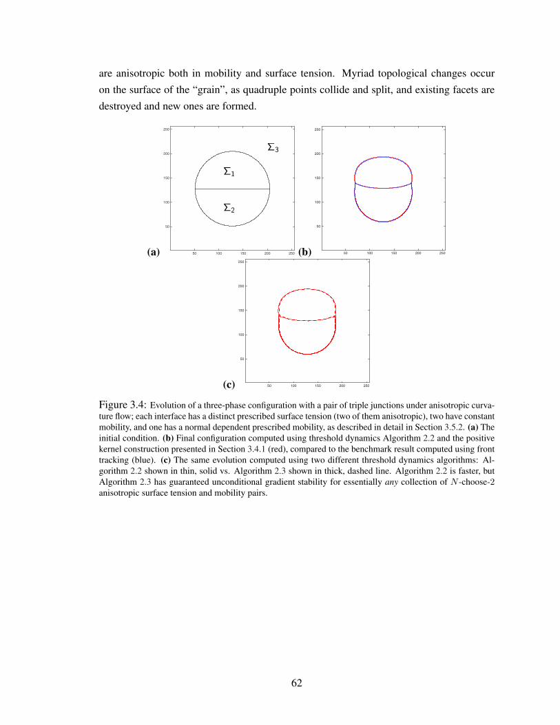
are anisotropic both in mobility and surface tension. Myriad topological changes occuron the surface of the “grain”, as quadruple points collide and split, and existing facets aredestroyed and new ones are formed.
(a) 50 100 150 200 250
50
100
150
200
250
(b) 50 100 150 200 250
50
100
150
200
250
(c) 50 100 150 200 250
50
100
150
200
250
Figure 3.4: Evolution of a three-phase configuration with a pair of triple junctions under anisotropic curva-ture flow; each interface has a distinct prescribed surface tension (two of them anisotropic), two have constantmobility, and one has a normal dependent prescribed mobility, as described in detail in Section 3.5.2. (a) Theinitial condition. (b) Final configuration computed using threshold dynamics Algorithm 2.2 and the positivekernel construction presented in Section 3.4.1 (red), compared to the benchmark result computed using fronttracking (blue). (c) The same evolution computed using two different threshold dynamics algorithms: Al-gorithm 2.2 shown in thin, solid vs. Algorithm 2.3 shown in thick, dashed line. Algorithm 2.2 is faster, butAlgorithm 2.3 has guaranteed unconditional gradient stability for essentially any collection of N -choose-2anisotropic surface tension and mobility pairs.
62

50 100 150 200 250
50
100
150
200
250
50 100 150 200 250
50
100
150
200
250
50 100 150 200 250
50
100
150
200
250
Figure 3.5: The Wulff shapes corresponding to the anisotropies used in the triple junction example. Fromleft to right: Wσ1,2 , Wσ1,3 , and Wσ2,3 .
Figure 3.6: Evolution of phase i = 1 out of a total of 27 phases, from two different simulations startingfrom the same initial condition. Top row: σi,j(θ, φ) = µi,j(θ, φ) = 1 for all i 6= j. Bottom row: σi,1(θ, φ) =1.1√
1 + 0.3 cos2 φ and µi,1(θ, φ) = 11.1
√1 + 0.3 cos2 φ for i 6= 1, and σi,j(θ, φ) = µi,j(θ, φ) = 1 for
i 6= 1 and j 6∈ i, 1. Many topological changes occur on the surface of the “grain”, where quadruple pointscan be seen to collide and split numerous times.
3.6 Conclusions
We have presented two simple and practical methods to construct convolution kernels tobe used in threshold dynamics schemes for curvature motion in two or three dimensions.Our constructions allow, for the first time, specifying a possibly anisotropic surface tensionand possibly anisotropic mobility simultaneously: these are encoded into the convolutionkernel. Combining the new kernel constructions with extensions of threshold dynamicsalgorithms presented in [26], we arrived at unconditionally gradient stable schemes forfully anisotropic, multiphase motion by weighted mean curvature of networks in two andthree dimensions. This level of generality allows specifying n-choose-2 anisotropic surfacetensions and n-choose-2 anisotropic mobilities for a network of n phases. Numerical ex-
63

periments indicate that in the multiphase setting, one of our new kernel constructions givessignificantly more accurate results than the other.
Along the way, our work has also elucidated necessary and sufficient conditions for thepositivity of the convolution kernel used in a threshold dynamics scheme in terms of thesurface tension and mobility factors of the desired weighted mean curvature flow.
64

CHAPTER 4
Auction Dynamics:A Volume Preserving MBO Scheme 3
4.1 Auction Dynamics
We now wish to extend the variational framework of the heat content energy to volumepreserving MBO schemes. Suppose we have a partition Σ where each phase has somevolumem(Σ`) = v` with respect to the Lebesgue measurem onD. We now wish to evolveΣ by curvature flow while keeping the volume of each phase fixed. The natural approach isto solve (2.29) with the additional constraint that the volume of each phase must stay fixed.Thus the thresholding step is instead replaced with the following minimization problem
arg minu∈KN
N∑`=1
∫D
ψk` (x)u`(x)dx s.t.∫D
u`(x)dx = v`. (4.1)
If we incorporate the volume constraints with a Lagrange multiplier λ we see that thesolution to (4.1) is a partition Σ given by a λ∗ shifted thresholding
Σi = x ∈ D : i = arg min1≤`≤N
ψ`(x)− λ∗i (4.2)
where λ∗ is the optimal Lagrange multiplier. It then follows essentially immediately from[74] that the scheme is consistent with volume preserving weighted curvature flow. Fur-thermore, if K ≥ 0 and the surface tensions σ satisfy a triangle inequality then the schemeis also unconditionally stable [27].
Now, there is a difficulty that we need to address. If N > 2, finding the optimalLagrange multiplier λ∗ is not trivial (if N = 2 one can find the multiplier by simply sortingthe convolution values). This task is particularly difficult if one insists on solving for the
3Joint work with Selim Esedoglu and Ekaterina Merkurjev [50].
65
Lagrange multiplier and the configuration Σ simultaneously (as we do). Our approach isto connect (4.1) to the assignment problem, a famous linear programming problem withefficient solutions. The assignment problem is typically posed as a maximization problem,thus as a first step we will replace (4.1) with the equivalent problem (4.3)
arg maxu∈KN
N∑`=1
∫D
a`(x)u`(x)dx s.t.∫D
u`(x)dx = v`, (4.3)
where a`(x) = (1− ψk` (x)). However, rather than working with problem (4.3) directly, wewill consider a discretized version. Discretization is natural, as any implementation of thescheme must be carried out on a finite grid. Discretization also allows us to more clearlyconnect our approach to the assignment problem, which is typically posed over a finitedimensional vector space. Let Dn = x1, . . . , xn ⊂ D be some n point discretizationof D. We discretize the volume constraints by requiring each phase to occupy V` points,where V` are integers chosen so that
∑N`=1 V` = n and the ratios V`/n ≈ v`/m(D) are as
close as possible. Since the convolution values a`(x) = (1− ψk` (x)) are smooth functions,they have a well defined restriction to Dn. Finally, the discrete analogue of KN is the setof functions u : Dn → [0, 1]N :
∑N`=1 u`(x) = 1, which may also be represented as
u ∈ [0,∞)n×N :∑N
`=1 u`(x) = 1. Using the latter representation we arrive at
arg maxu≥0
N∑`=1
∑x∈Dn
a`u`(x) s.t.∑x∈Dn
u`(x) = V`,N∑`=1
u`(x) = 1. (4.4)
In this form, problem (4.4) can be viewed as a special case of a family of linear pro-gramming problems. This family of problems stems from the minimum cost flow problem,and includes famous problems such as the assignment problem, the transportation problemand the maximum flow problem. We choose to focus on the assignment problem, as it isthe simplest of the problems and can be solved with an intuitive economic approach.
4.1.1 The assignment problem
Given two disjoint sets X and I of equal size r and a weight function w : X × I → R, theassignment problem seeks to find a one to one matching M = (x1, i1), . . . , (xr, ir) of Xand I (i.e. a bijection), such that the total weight of the matching∑
(x,i)∈M
wi(x) (4.5)
66

is maximized. By representing the matching as a binary vector z where zi(x) = 1 if(x, i) are matched and zi(x) = 0 otherwise, we can restate the assignment problem as thefollowing optimization problem
maxz:X×I→0,1
∑x∈X
∑i∈I
wi(x)zi(x) s.t.∑x∈X
zi(x) = 1,∑i∈I
zi(x) = 1. (4.6)
If we relax the binary constraint on z then (4.6) becomes the following linear programmingproblem
maxz≥0
∑x∈X
∑i∈I
wi(x)zi(x) s.t.∑x∈X
zi(x) = 1,∑i∈I
zi(x) = 1. (4.7)
It turns out that the relaxation is exact, and we may substitute (4.7) for (4.6). This fol-lows from the fact that the solution to a bounded and feasible linear programming problemalways includes a vertex of the feasible polytope. The relaxed linear constraint set is thepolytope z ≥ 0 :
∑x∈X zi(x) = 1,
∑i∈I zi(x) = 1. The vertices of the polytope are
precisely the vectors z whose entries are binary.Now observe that problem (4.4) is a special case of (4.7), with respect to a particular
choice of weights wi(x). We can obtain (4.4) from a generic instance of (4.7) by lettingX = Dn splitting I into N similarity classes S`N`=1 each of size V` and setting wi(x) =
a`(x) for every i ∈ S`. With those choices (4.7) becomes
maxz≥0
∑x∈Dn
N∑`=1
a`(x)∑i∈S`
zi(x) s.t.∑x∈Dn
zi(x) = 1,∑i∈I
zi(x) = 1. (4.8)
Now if we define u`(x) =∑
i∈S` zi(x), we can relax the constraints to∑
x∈Dn u`(x) = V`
and∑N
`=1 u`(x) = 1 without changing the value of the problem. Thus (4.4) can be obtainedas a special case of (4.7). In fact, the two problems are actually equivalent, a genericinstance of (4.4) can also be transformed into a specific instance of (4.7).
For the remainder of this chapter we will focus on our special case (4.4) of the assign-ment problem (see [10] for a similar discussion of the classic formulation (4.7)). We willinterchangeably represent matchings as vectors u in the feasible polytope and as partitionsΣ = (Σ1, . . . ,ΣN) of Dn. Our goal for the remainder of this subsection is to develop anintuition for (4.4), and develop the necessary setup for the auction algorithm in Section4.1.2.
It is particularly instructive to give a practical interpretation of (4.4). Imagine thateach phase is an institution that offers a limited number of memberships. For example,the phases may be gyms, or clubs, or different Costco locations, etc. Imagine that thepoints x ∈ Dn are people, and each person would like to become a member of some
67

phase. No person wants to have a membership in more than one phase, and each phaseonly has V` memberships available. Finally, imagine that the coefficients a`(x) representhow much person x wants to be a member of phase `. Now we can think of the solutionto the assignment problem as the matching of people and phases that maximizes the totalsatisfaction of the population. Ideally, each person would like to become a member of theirfavorite phase. However, this is not possible if more than V` people want to be members ofsome phase `. The main difficulty of the assignment problem is in understanding how tocorrectly handle these conflicts.
An interesting approach is to attempt to assign the memberships according to a marketmechanism. Imagine that each phase ` has a membership price p`, and if person x is amember of ` then they must pay p`. This can help to resolve conflicts by making the mostpopular phases more expensive. Assuming that every person acts in their own best interest,x will want to buy a membership at the phase offering the best value, i.e. x wants to be amember of any phase
`∗ ∈ `cs(x,p) = arg max1≤`≤N
a`(x)− p`. (4.9)
We are now led to a very interesting question: does there exist an equilibrium price vectorp∗ such that assigning memberships according to (4.9) gives a feasible matching? Theanswer to this question is yes, and better yet the resulting assignment is optimal.
The connection between the assignment problem and the equilibrium price vector p∗comes from the duality theory of linear programming. As it turns out, the equilibrium pricep∗ is in fact the optimal solution to the dual of the assignment problem. In addition to theprices p, the dual problem introduces a set of variables π(x) for each x ∈ Dn. The dualproblem is
minp∈RN ,π∈Rn
N∑`=1
pi +∑x∈Dn
π(x) s.t. π(x) + p` ≥ a`(x). (4.10)
Note that the optimal value of π is entirely determined by p. Given any p the best choicefor π is to set π(x) = max1≤`≤N a`(x) − p`. This shows that π(x) is exactly the value ofthe best deal offered to x by any phase.
Our earlier statements about the equilibrium price vector p∗ can be justified by invokingthe complementary slackness (CS) condition. According to CS, a feasible assignment uand a feasible dual pair (p,π) are optimal for their respective problems if and only if
∑x∈Dn
N∑`=1
u`(x)(p` + π(x)− a`(x)) = 0. (4.11)
Recalling the best choice for π, (4.11) implies that in the optimal matching every person
68

is assigned a membership which satisfies the market strategy (4.9) using the optimal pricevector pc. This implies that the equilibrium price p∗ exists and p∗ = pc.
Now suppose that we have some price vector p which is not optimal for the dual prob-lem. By CS, it will not be possible to assign every membership according to (4.9), therewill necessarily be conflicts. However, we can attempt to construct a partial assignment(partial matching). A partial assignment matches a subset of people in S ⊂ Dn to phases1, . . . , N while ensuring that no more than V` people are assigned to any phase. A partialmatching can be represented as a partition Σ of S into N phases Σ = (Σ1, . . . ,ΣN) suchthat |Σ`| ≤ V` for every phase `. Given a partial matching Σ, if x ∈ Σ` then it will benotationally convenient to say that the pair (x, `) is in the matching. A partial assignmentΣ and a price p satisfies CS if for every phase ` and every member x ∈ Σ` the pair (x, `)
satisfies (4.9).The most efficient algorithms for the assignment problem have the same basic structure.
They generate a sequence of price vectors pk and partial matchings Σk such that Σk andpk satisfy CS. Each stage of the algorithm either increases the size of the partial matching(a larger subset of Dn matched) or improves the prices (with respect to the dual problemvalue). Since CS is preserved at every step, if the partial matching becomes a completematching then it is an optimal solution to the assignment problem.
We will solve the assignment problem using auction algorithms. Auction algorithmshave a simple intuitive structure, are easy to code, and have excellent performance. Themain advantage of auction algorithms over the well-known Hungarian algorithm [53, 68]isthat auction algorithms perform local modifications of Σk and pk at every step, whereasthe Hungarian algorithm may need to consider global modifications.
4.1.2 Auction algorithms
In [9] Bertsekas developed the auction algorithm for solving the classic assignment prob-lem (4.7). Since the original paper, Bertsekas and collaborators have improved upon thecomputational aspects of the auction algorithm, and extended it to more general minimumcost flow problems (see [11] or [10] for an exhaustive reference on auction algorithms).The most important references for this work are [12] and [13]. In [12] Bertsekas and Cas-tanon modified the auction algorithm to more efficiently handle assignment problems withmultiple identical objects as in (4.4). In [13], Bertsekas, Castanon, and Tsaknakis intro-duced the reverse auction algorithm for asymmetric assignment problems, which we willuse in Section 4.1.3.
The basic idea of the auction algorithm is to drive price modifications and augmenta-
69

tions of the partial matching by simulating an auction. In order to obtain a membership,each person x must submit a bid b(x) to the phase of their choice. At the start of the auc-tion, the price of a membership at each phase ` is set to a starting value p0
` according tosome initial price vector p0. As in a real life auction, if a person x submits a bid b(x) to aphase ` the bid must exceed or match the current price p`. Using the CS condition (4.9), wecan split the phases into three sets, the high demand phases H , the low demand phases L,and the equilibrium phases E. The high demand phases ` ∈ H have more than V` peoplewho would like to purchase a membership, the low demand phases ` ∈ L have fewer thanV` people and the equilibrium phases ` ∈ E have exactly V` people. Everyone who wants alow demand or equilibrium membership can submit a bid and immediately be accepted intothe initial partial matching, but there is a conflict at the high demand phases. The conflictis resolved by choosing the people who have submitted the largest bids. At any step of thealgorithm, if ` is a high demand phase then the set Σ` consists of the V` people who havesubmitted the largest bids for phase `. As people submit bids, the prices of the high demandphases will rise. Eventually, this will incentivize unmatched people to switch their bid to acheaper phase that may offer a better bang for their buck. The algorithm terminates onceall of the phases are in equilibrium.
Now we need to discuss pricing and bidding strategies. Each phase is restricted tosetting one uniform membership price, regardless of how large individual bids may be.Assuming that a phase does not want to lose members, the price should be set to the amountthat the least committed member is willing to pay. This amount is the lowest bid that a phasereceived thus far. To make this strategy consistent across all phases, assume that the emptyspots in every low demand phase ` ∈ L are filled by phantom members who all bid thestarting price p0
` .Finding a bidding strategy that guarantees termination of the algorithm and produces
a complete matching satisfying CS turns out to be nontrivial. For a given price vector p,if person x is a member of phase ` then we must have ` ∈ `cs(x,p) to satisfy CS. Thissuggests that in the course of the auction, an unmatched person x should only submit bidsto phases in `cs(x,p). The subtlety lies in the question, ‘How much should person x bewilling to bid?’ Obviously, x does not want to overbid, otherwise prices may rise anda different phase will become optimal according to CS. The largest bid, b(x), that x cansubmit to `∗ ∈ `cs(x,p) while being guaranteed not to violate CS is
b(x) = p`∗ + (a`∗(x)− p`∗)− (a`next(x)− p`next) (4.12)
70

where`next ∈ arg max
j 6=`∗a`(x)− p` (4.13)
is x’s second most desirable phase. With this bid, x is willing to allow the price of `∗ toincrease to at most the gap in value between the best and second best choice. While x ismatched to `∗, the price p`∗ cannot increase beyond b(x). Other prices are non-decreasing,thus for the duration that (x, `∗) is part of the partial matching, this pair satisfies CS.
Unfortunately, this bidding strategy does not work. A problem occurs when there aremultiple optimal objects for x, i.e. when |`cs(x)| > 1. If this happens then both `∗, `next ∈`cs(x,p) and thus the gap (a`∗(x)− p`∗)− (a`next(x)− p`next) = 0. In this case x is unable toraise the price of `∗. This situation may lead to a price war. In a price war, multiple peoplecompete for the same memberships without ever raising the prices, trapping the algorithmin an infinite loop.
To circumvent this difficulty, one must relax the complementary slackness condition.For a given price vector p and a small ε > 0 a matched pair (x, `) satisfies the ε-complementaryslackness condition (ε-CS) if
a`(x)− p` + ε ≥ max1≤j≤N
a`(x)− p`. (4.14)
It is now possible to create a bidding strategy that preserves ε-CS and guarantees thatthe algorithm will always terminate. As before, an unmatched x will only submit bids to`∗ ∈ `cs(x,p), however now x can bid up to
b(x) = p`∗ + ε+ (a`∗(x)− p`∗)− (a`next(x)− p`next) (4.15)
without overpaying according to ε-CS. Since (a`∗(x) − p`∗) − (a`next(x) − p`next) ≥ 0 thisensures that p`∗ increases by at least ε. This mimics real life auctions where any bid mustbe larger than the current price by at least some fixed amount. Now starting from any initialprice vector p0 the algorithm will be guaranteed to eventually terminate [9]. We now giveour version of the auction algorithm, which is equivalent to the “similar object” auction
71

variant in [12].Algorithm 4.1: Membership Auction [12]
Input: ε > 0, volumes V , coefficients a, initial prices p0 and people x ∈ Dn
Result: Final prices and complete ε-CS matching (Σ,p).Initialization: For every ` ∈ 1, . . . , N mark all x as unassigned, set p = p0, setΣ = ∅ ;
while some x is marked as unassigned dofor each unassigned x ∈ Dn do
Calculate `cs(x,p) and choose some `∗ ∈ `cs(x,p);Set b(x) = p`∗ + ε+ (a`∗(x)− p`∗)− (a`next(x)− p`next);if |Σ`∗| = V`∗ then
Find y = arg minz∈Σ`∗b(z);
Remove y from Σ`∗ and add x to Σ`∗;Mark y as unassigned and mark x as assigned;Set p`∗ = minz∈Σ`∗ b(z);
elseMark x as assigned and add x to Σ`∗;if |Σ`∗| = V` then
Set p`∗ = minz∈Σ`∗ b(z);end
endend
endreturn (Σ,p)
The output of the auction algorithm is a complete matching Σ satisfying ε-CS, and thefinal auction prices p. Representing the matching as a binary vector u and using ε-CS wemay conclude
N∑`=1
p` +∑x∈Dn
max1≤`≤N
[a`(x)− p`] ≤ nε+∑x∈Dn
N∑`=1
u`(x)a`(x). (4.16)
Thus, by weak duality, the final assignment u is at most nε away from being optimal. Inthe special case where the coefficients a`(x) integers, an ε-CS matching is actually optimalfor any ε < 1
N[12].
We now give a quick sketch of the complexity. Assume that at the start of the auc-tion the prices were initialized to zero and the partial matching was empty. Let C =
72

max`∈1,...,N,x∈Dn
a`(x) be the largest coefficient. Suppose in the course of the algorithm that
the price of some phase ` exceeds C. If the algorithm has not yet terminated then theremust be some low demand phase with price zero. This implies that in the remainder of theauction no person x will ever bid on phase ` again, since there must be a phase offeringa better value. Thus we have an upper bound on the price of any phase. Suppose thatsome phase ` is currently priced at p`, and consider the number of bids required to raise theprice. The worst possible case occurs when every currently matched member has bid ex-actly p` (such a situation is highly degenerate and rarely appears in practical applications).In this case it will take exactly V` bids to raise the price. The price must rise by at least ε,thus, we can conclude that the algorithm will terminate after at most NV dC/εe bids whereV = max1≤`≤N V`.
A straightforward implementation of the bidding steps in Algorithm 4.1 requiresO(V +
N) operations. This can be sped up with special data structures. If we implement a priorityqueue for each Σ` we can complete a bid in O(log(V ) +N) operations. In all of our appli-cations V is several orders of magnitude larger thanN , thus this gives considerable savings.Combining this with the estimate for the maximum number of bids we can conclude thealgorithm has complexity O
(NV (log(V ) + N)C/ε
). Note that due to the presence of the
constant C this complexity is pseudo-polynomial rather than polynomial.The complexity can be improved using the idea of epsilon scaling (noted in [9] and
analyzed in [36, 37, 38]). Suppose that (Σ′,p′) is a matching and a price vector satisfyingrε-CS for some r > 1. What happens if we use p′ as the initial price vector when we runthe auction algorithm with ε? Since any starting price is admissible, the algorithm will stillproduce a matching and price (Σ,p) satisfying ε-CS. However, if r is not too large thenwe should expect that p′ and p are not too different. This suggests that the auction willnot need to modify the prices very much, and thus the algorithm will terminate quickly.Epsilon scaling takes advantage of this idea by running the auction multiple times withsuccessively smaller values of epsilon. The final price vector of the previous run is usedas the initial price vector in the next run. Typically, one takes the sequence of decreasingepsilon values to be εk = C/αk for some integer α > 1, stopping once εk < δ
nfor some
small δ. Using ε scaling the complexity can be improved to a weakly polynomial bound.We refer our readers to [11] for the exact details and bounds using ε-scaling. For theproblems that we consider, the complexity of the auction algorithm using ε-scaling appearsto grow like O
(NV (log(V ) + N) log(nC/δ)
)(see [10] or [11] for a heuristic explanation
of this behavior).Now we are ready to give the auction dynamics algorithm, Algorithm 4.2. Recall that
our goal is to simulate the evolution of a configuration Σ under volume preserving curva-
73

ture flow for some time t = m(δt). As we saw in the beginning of Section 4.1 we obtain aconsistent and unconditionally stable scheme by solving the iteration
Σk+1 = arg minΣ
Lδt(Σk,Σ) s.t. |Σ`| = V` for 1 ≤ ` ≤ N (4.17)
m times. This amounts to repeatedly taking convolutions of the configuration Σk with akernel K, and solving the assignment problem. As we have seen above, we can solve theassignment problem efficiently using auctions. Auction dynamics uses Algorithm 4.1 alongwith ε-scaling to quickly and accurately obtain a solution. We give the algorithm below.
Algorithm 4.2: Auction DynamicsInput: Discrete domain Dn, initial configuration Σ, surface tensions σ, convolution
kernel K, volumes V , time step δt, number of steps m, auction errortolerance εmin, epsilon scaling factor α, initial epsilon value ε0.
Result: Final configuration Σm
Initialization: Set Σ0 := Σ, set ε = εmin/n;for k from 0 to m− 1 do
Calculate the convolutions: ψk+1` (x) =
∑j 6=` σ`j(Kδt ∗ Σk
j )(x);Calculate the assignment problem coefficients: ak+1 = 1−ψk+1;Initialize prices p = 0, and ε = ε0;while ε ≥ ε do
Run Algorithm 4.1 (Membership Auction):(Σout,pout) = Membership Auction(ε,V ,ak+1,p, Dn);
Set p = pout;Divide ε by α;if ε < ε then
Set Σk+1 = Σout;end
endendreturn Σm
4.1.3 Upper and lower volume bounds
In addition to strict volume preserving curvature flow, auction dynamics can be modified toallow the volume of each phase to fluctuate between some bounds. This will be particularlyuseful in our applications to machine learning.
Suppose that each phase ` must have at least B` members and at most U` members for
74

some integers B` and U`. To ensure that the resulting problem is feasible we will requireB` ≤ U` and
∑N`=1B` ≤ n ≤
∑N`=1 U`. We will then need to solve the following modified
version of the assignment problem
maxu≥0
N∑`=1
∑x∈Dn
a`(x)u`(x) s.t.N∑`=1
u`(x) = 1, B` ≤∑x∈Dn
u`(x) ≤ U`. (4.18)
This version of the problem introduces some complexities that were not present in (4.4)and will require a more sophisticated approach.
Previously, we examined and solved the assignment problem from the perspective ofthe people x ∈ Dn. The limited supply of memberships resulted in competition betweenthe people, which we resolved by introducing prices and simulating an auction. The upperbounds fit nicely into this perspective. The upper bounds indicate that each phase has alimited number of memberships, however it is now possible that the total supply of mem-berships
∑N`=1 U` exceeds the number of people n. The upper bounds will still induce
competition between the people, but the oversupply of memberships means that the set ofequilibrium prices will be larger. This will add a wrinkle of difficulty, as not all equilibriumprices will be dual optimal.
The lower bounds are fundamentally different and require a new perspective. Indeed,if some person x sees that there is an available membership in their most desirable phase `,they will immediately join ` without caring if some other phase j is deficient (i.e. |Σj| <Bj). Instead, we must think about the lower bounds from the perspective of the phases.Imagine that each phase must sell B` memberships or they will go out of business. If aphase ` is having trouble attracting a sufficient number of people, it will have to introducean incentive t` to entice people to join. As a result, the lower bounds induce a competitionamong the phases. Deficient phases will be forced to offer competing incentives to attractthe necessary number of members. Thus, in order to satisfy the lower bounds, we will needto run a reverse auction [13] where the phases bid on the people.
To properly understand the interaction between the prices and incentives, we introducethe dual problem
minp≥0,t≥0,π∈Rn
N∑`=1
p`U` − t`B` +∑x∈Dn
π(x) s.t. p` − t` + π(x) ≥ a`(x). (4.19)
As before, we will use the interplay between the primal and dual problems to drive thesearch for the optimal solution. The key of course will be the complementary slacknesscondition. The complementary slackness condition for (4.18) and (4.19) states that an
75

assignment u and dual variables (p, t,π) are optimal for their respective problems if andonly if
N∑`=1
∑x∈Dn
u`(x)(a`(x)− p` + t` − π(x))
+N∑`=1
p`(U` −∑x∈Dn
u`(x)) +N∑`=1
t`(∑x∈Dn
u`(x)−B`) = 0.
(4.20)
Recall that π is determined by p and t and is given by π(x) = max1≤`≤N a`(x) + t` − p`.Now we can recognize that the complementary slackness condition has a simple intuitiveexplanation. The first sum states that each person should be assigned to the optimal phasebased on prices and incentives (this should feel familiar). The second sum states that phasescharging membership prices must have the maximum number of members U` (i.e. nooverpriced phases). Similarly, the third sum states that the phases offering incentives musthave the minimal number of members B` (i.e. no over-incentivized phases).
To ensure our auctions do not stall, we will once again turn to the ε-CS condition. Forthis problem, we will say that a partial matching Σ and a price-incentive pair (p, t) satisfyε-CS if every matched pair (x, `) satisfies
a`(x)− p` + t` + ε ≥ max1≤j≤N
aj(x)− pj + tj. (4.21)
As before, we can recognize this ε-CS condition as an ε relaxed version of the first sum in(4.20). Unfortunately, the other two terms in (4.20) do not have useful ε relaxations. Asa result, we will need to carefully ensure that our auctions will satisfy the other two termsexactly. We will say that a price p (an incentive t) is admissible for a matching Σ if thesecond (third) term of (4.20) is satisfied.
We will solve (4.18) in two stages. First we will run Algorithm 4.3, a forward auctionalgorithm similar to Algorithm 4.1, where the people compete for memberships. This willproduce a complete ε-CS matching satisfying the upper bound constraints but possiblyviolating the lower bound constraints (we will call this upper feasible). Algorithm 4.3differs from Algorithm 4.1, as it simultaneously runs a mechanism to ensure that no phaseis over-incentivized. In the second stage we will feed the result of the first stage into areverse auction, Algorithm 4.4, where the phases compete for people. This will produce anε-CS matching that is both upper and lower feasible. In addition, Algorithm 4.4 will havea mechanism to prevent phases from becoming overpriced. As a result, the final outputwill be a complete and feasible ε-CS matching Σ with admissible prices and incentives(p, t). This will be enough to conclude that Σ solves (4.18) with error at most nε. In the
76

special case that the coefficients a are all integers, the argument used in [12] can be easilygeneralized to show that the solution is optimal if ε < 1
N.
Algorithm 4.3 is a relatively straightforward adaptation of the similar object auctionsand the asymmetric assignment auctions found in [11]. On the other hand, Algorithm 4.4appears to have a different structure than the reverse auctions considered in [11]. Indeed,in our reverse auction we choose to work with prices and incentives rather than the profitvariable π. We find that working with prices and incentives leads to a much faster runtimewhen N << n. Since both algorithms are highly specialized for our current problem, weprovide proofs that they terminate and have the desired properties.
Algorithm 4.3: Upper Bound AuctionInput: ε > 0, boundsB,U , coefficients a, initial prices p0, initial incentives t0 and
people x ∈ Dn
Result: Prices p, admissible incentives t, and complete ε-CS matching Σ satisfyingupper bounds.
Initialization: Mark all x as unassigned, set d = p0 − t0, set Σ = ∅ ;while some x is marked as unassigned do
for each unassigned x ∈ Dn doCalculate `cs(x,p) and choose some `∗ ∈ `cs(x,d);Set b(x) = d`∗ + ε+ (a`∗(x)− d`∗)− (a`next(x)− d`next);if |Σ`∗| = U`∗ then
Find y = arg minz∈Σ`∗b(z);
Remove y from Σ`∗ and add x to Σ`∗;Mark y as unassigned and mark x as assigned;Set d`∗ = minz∈Σ`∗ b(z);
else if |Σ`| = B` and d` < 0 thenFind y = arg minz∈Σ`∗
b(z);Remove y from Σ`∗ and add x to Σ`∗;Mark y as unassigned and mark x as assigned;Set d`∗ = min(minz∈Σ`∗ b(z), 0);
elseMark x as assigned and add x to Σ`∗;
endend
endSet p = max(d,0), set t = max(−d,0);return (Σ,p, t)
77

Proposition 4.1.1. Given initial prices and incentives p0, t0, and an empty matching, Al-
gorithm 4.3 produces an upper feasible ε-CS matching Σ with no over-incentivized phases
with time complexity O(NU(log(U) + N)(C + G)/ε) where U = max1≤`≤N U` and
G = max1≤`,j≤N(p0j − t0j)− (p0
` − t0`).
Proof. Note that no phase can increase beyond U` members, and no phase can increase be-yond B` members as long as d` < 0. Therefore, the algorithm will not terminate until thematching is complete, upper feasible, and there are no over-incentivized phases. Through-out the auction the number of unmatched people is non-increasing and the variable d isentrywise non-decreasing. The monotonicity of these quantities allows us to use the samecomplexity argument as in Algorithm 4.1. The above bound will then immediately follow,where the factor G accounts for the prices and incentives not being initialized to zero.
It remains to show that the algorithm preserves ε-CS at every step. The only placewhere this algorithm differs from Algorithm 4.1 is when a person x wants to join a phase` where |Σ`| = B` and d` < 0. Let d,d′ be the values before and after x is added. Sinced′` ≤ miny∈Σ` b(y) every person matched to ` must satisfy ε-CS.
78

Algorithm 4.4: Lower Bound AuctionInput: ε > 0, boundsB,U , coefficients a, initial prices p0, initial admissible
incentives t0, complete (but possibly lower infeasible) ε-CS matching Σ0
Initialization: Set d = p0 − t0, set Σ = Σ0 ;Result: complete and feasible ε-CS matching and admissible prices and admissible
incentives (Σ,p, t).while there exists some ` with (|Σ`| < U` and d` > 0) or (|Σ`| < B`) do
for each `∗ with (|Σ`∗| < U`∗ and d`∗ > 0) or (|Σ`∗| < B`∗) dofor each x /∈ Σ`∗ do
Let j be x’s current phase;Calculate ∆(x) = (aj(x)− dj)− (a`∗(x)− d`∗);
endwhile (|Σ`∗| < U`∗ and d`∗ > 0) or (|Σ`∗| < B`∗) do
Find x ∈ arg miny/∈Σ`∗∆(y);
if |Σ`∗| < B`∗ thenRemove x from its current phase and add x to Σ`∗;if |Σ`∗| = B`∗ and ∆(x) ≥ 0 then
Subtract ∆(x) + ε from d`∗;end
elseif ∆(x) + ε ≥ d`∗ then
Set d`∗ = 0;else
Remove x from its current phase and add x to Σ`∗;if |Σ`∗| = U`∗ and ∆(x) ≥ 0 then
Subtract ∆(x) + ε from d`∗;end
endend
endend
endSet p = max(d,0), set t = max(−d,0);return (Σ,p, t)
Proposition 4.1.2. Given the result of Algorithm 4.3, Algorithm 4.4 produces a complete
79

and feasible ε-CS matching Σ with no overpriced or over-incentivized phases with time
complexity O(n2N2(C +G)/ε) where G = max`6=j(p0j − t0j)− (p0
` − t0`).
Proof. It is clear that the algorithm will not terminate until the matching is complete andlower feasible, and there are no over-priced phases. The algorithm will never add peopleto an already full phase ` with |Σ`| = U`, thus the matching stays upper feasible. A phaseonly offers incentives if it has fewer than B` members, and any phase that has offeredan incentive will never have more than B` members. Thus, no phase will become over-incentivized.
Next, we show that Σ is a complete ε-CS matching at every step of the algorithm.Consider what happens when a phase `∗ is modified. Let (Σ,d) the values before themodification and (Σ′,d′) afterwards.
First, we consider the case where |Σ`∗| < B`∗ . In this case Σ′`∗ must now have B`
points. Let xf be the last point added to `∗. If d′`∗ = d`∗ then ∆(xf ) < 0 and we canconclude that every person who had their membership switched to `∗ strictly preferred `∗
over their previous membership. Since no other entry of d changed, the new pair (Σ′,d′)
still satisfies ε-CS. Otherwise, ∆(xf ) ≥ 0 and d′` = d`−∆(xf )− ε. Clearly everyone whowas in Σ` is even happier to be in Σ′`∗ as d′`∗ < d`∗ and other entries of d didn’t change.Next, we check the other people whose membership didn’t change. Let y be some persony ∈ Σ′j for some j 6= `∗. We need to show that max1≤`≤N a`(y) − d′` − ε ≤ aj(y) − d′j .Only d′`∗ is different so it is enough to show a`∗(y)− d′`∗ − ε ≤ aj(y)− dj . By our choiceof xf we have
a`∗(y)− d′`∗ − ε = a`∗(y)− d`∗ + ∆(xf ) ≤ a`∗(y)− d`∗ + ∆(y) = aj(y)− dj.
Finally we check the people who were switched to `∗. Let z be one of those people andsuppose that z was previously matched to phase r. Since ∆(xf ) ≥ ∆(z) we may conclude
max6=`∗
a`(z)− d′` ≤ ar(z)− dr + ε = a`∗(z)− d`∗ + ε+ ∆(z) ≤ a`∗(z)− d′`∗ .
Next, we consider the case where |Σ`∗| < U`∗ and d`∗ > 0. This case is very similar,however there is one additional thing that can happen. Namely, it is possible that d′`∗ canbe set to zero before Σ′`∗ reaches U`∗ members. As before, let xf be the last person addedto `∗ in the modification, and let yc = arg miny/∈Σ′`
∆(y). If xf exists (possibly no one wasadded) then ∆(xf ) + ε < d`∗ ≤ ∆(yc) + ε. Similar arguments to the above now show thatanyone in Σ′`∗ satisfies ε-CS. To check that every other person satisfies ε-CS it is enough to
80

show that yc satisfies ε-CS. Suppose that yc is matched to a phase j. Then
a`∗(yc)− d′`∗ ≤ a`∗(yc) + ∆(yc) + ε− d`∗ = aj(yc)− dj + ε
which is enough to show ε-CS for yc. Thus the algorithm preserves ε-CS.Finally, we show that the algorithm terminates. Suppose for some ` the quantity d`
decreases by more than 2(C +G) + ε from its starting value. Since d0` −G ≤ 0 it must be
the case that |Σ`| ≤ B`. Immediately after d` is lowered to d0` − C − 2G− ε phase ` must
have exactly B` members. If the algorithm has not terminated then there must be some jwith more than Bj members, and thus dj ≥ d0
j −G. For any x we can then conclude that
a`(x)− d` − (aj(x)− dj) ≥ a`(x)− aj(x) + d0j − d0
` + 2C +G ≥ 0.
It then follows that |Σ`| = B` for the remainder of the auction, as it will always be easierfor other phases to incentivize people to leave phase j rather than phase `.
Notice that the same person cannot switch phases N times unless one of the entries ofd has decreased. Thus, a phase ` can enter a bidding stage at mostNn times before d` mustdecrease by at least ε. This gives us an upper bound of 2N2nd(C +G)/εe bidding stagesbefore the algorithm terminates. Quickselect (a variant of Hoare’s quicksort algorithm) canbe used to find the k smallest values of ∆(x) in time O(n) regardless of k [45]. Thus theworst case complexity of the algorithm is O(n2N2(C +G)/ε).
Both Algorithms 4.3 and 4.4 are compatible with ε scaling. The prices and incentivesobtained from one iteration of Algorithms 4.3 and 4.4 together can be fed into the nextiteration. For the instances of (4.18) that we encounter, the complexity of both algorithmsusing ε scaling appears to grow like O(nN(log(n) + N) log(nC/δ)), where δ > 0 is themaximum error of the final solution.
With the upper and lower bound auction algorithms in hand, we can now give the ver-
81

sion of auction dynamics with upper and lower volume bounds, Algorithm 4.5 below.Algorithm 4.5: Auction Dynamics with Volume Bounds
Input: Domain Dn, initial configuration Σ, surface tensions σ, kernel K, volumeboundsB,U , time step δt, number of steps m, auction error tolerance εmin,epsilon scaling factor α, initial epsilon ε0.
Result: Final configuration Σm
Initialization: Set Σ0 := Σ, set ε = εmin/n;for k from 0 to m− 1 do
Calculate the convolutions: ψk+1` (x) =
∑j 6=` σ`j(Kδt ∗ Σk
j )(x);Calculate the assignment problem coefficients: ak+1 = 1−ψk+1;Initialize prices p = 0, incentives t = 0, and ε = ε0;while ε ≥ ε do
Run Algorithm 4.3 (Upper Bound Auction):(Σout1,pout1, tout1) = Upper Bound Auction(ε,B,U ,ak+1,p, t, Dn);
Run Algorithm 4.4 (Lower Bound Auction): (Σout2,pout2, tout2) =
Lower Bound Auction(ε,B,U ,ak+1,pout1, tout1,Σout1);Set (p, t) = (pout2, tout2);Divide ε by α;if ε < ε then
Set Σk+1 = Σout2;end
endendreturn Σm
4.1.4 Auction dynamics with temperature
Finally, we conclude this section with a variant of the auction dynamics algorithm that al-lows us to incorporate random fluctuations due to temperature. There are several reasonsto introduce temperature effects into auction dynamics, two of these are: 1. In machinelearning applications, temperature can help the algorithm escape from local minima andfind better solutions. 2. Low temperature levels can be added to auction dynamics tohelp avoid degenerate auction coefficients (which slow down the algorithm) without signif-icantly changing the result.
In the classic threshold dynamics algorithm, one may incorporate temperature in thestyle of rejection free Monte Carlo methods by randomizing the thresholding step. The
82

Monte-Carlo approach suggests randomly assigning each x to a phase i with probability:
P(x ∈ Σk+1i ) =
e−βψk+1i (x)∑N
j=1 e−βψk+1
j (x), (4.22)
where β = 1T
is the inverse temperature. In the limit as T → 0 one recovers the originalMBO algorithm.
Unfortunately this approach is not compatible with auction dynamics. The volume con-straints prevent us from assigning points independently. As a result, we cannot introducethe randomness in the assignment step. Instead, we introduce temperature before the as-signment step by perturbing the coefficients a`(x) = (1− ψ`(x)). Given some probabilitydistribution X = X(0, T ) on the reals with mean zero and variance T , we perturb eachcoefficient a`(x) by an independent sample of X . This approach maintains the same basicproperties as the randomness strategy (4.22). As T → 0, we recover the original algorithmand as T →∞ the points are assigned to phases completely randomly. In our implementa-tions of temperature effects, we choose the random variables to be normal random variablesN(0, T ).
4.2 Curvature motion
We demonstrate the effectiveness of our auction dynamics code by computing several ex-amples of volume preserving mean curvature motion in two and three dimensions. Sincethe focus of this work is to develop the necessary theory and algorithms for the volume con-strained case, we work with essentially the most basic implementation of auction dynamicswith the exception of the following well-known and simple trick to enhance the spatialresolution. The intermediate steps arising in each iteration of auction dynamics yields asmooth level set function (given by ψ − p) that can be used (via interpolation) to estimatethe fraction of each grid cell occupied by a given phase. This allows for a sub-pixel accu-rate representation of the characteristic functions of the phases. For applications requiringgreater efficiency or accuracy, one may turn to more sophisticated techniques developedfor threshold dynamics, which in principle extend to auction dynamics as well.
We begin by considering two different equal volume tessellations of the torus. In Fig-ure 4.1, the starting configuration is 64 randomly shifted squares of equal volume. Afterevolving under auction dynamics, the final configuration is a hexagonal lattice, which hasoptimal isoperimetric quotient among all equal volume tilings of the plane [41]. Thus, thealgorithm finds the lowest energy state as one would hope. A more interesting example is
83

given in Figure 4.2. The starting configuration consists of 17 equal volume rectangles. Inthe case of 17 subunits, it is impossible to tile the torus with hexagons [59]. Indeed, thefinal configuration contains a heptagon and a pentagon. Nevertheless, most of the shapesare hexagons and visual inspection suggests that all of the triple junction angles are nearly120 degrees. Therefore, the final configuration is a plausible minimizer of the interfacialperimeters.
Figure 4.1: Initial condition: Randomly shifted 8 columns of 8 squares that have identical areas. Periodicboundary conditions.
Next, we consider random Voronoi diagrams in 2 and 3 dimensions. Figure 4.3 depictsthe evolution of a random Voronoi diagram in the plane. The network immediately un-dergoes topological changes – all of quadruple junctions in the initial configurations splitand form triple junctions. Figure 4.4 shows the evolution of a single “grain” in a ran-dom Voronoi diagram in 3 dimensions, Figure 4.5 shows the same grain and several of itsneighbors at the final time. One can clearly see many topological changes in the faces of
84

Figure 4.2: Initial condition: Randomly shifted 17 rectangles that have identical areas. Periodic boundaryconditions. After a long time, there is still one phase with five and another with seven neighbors.
the grain. Quadruple junctions split and collide throughout the evolution. Both examplesclearly show that one must anticipate topological changes in the course of the flow.
Finally, we consider equal volume tilings in 3 dimensions. Our starting configurationis a randomly shifted cubic lattice with 8 phases. Unlike the two dimensional case above,where the flow easily found the optimal solution, the 3 dimensional energy landscape ap-pears to be littered with local minima. Regardless of how the cubes are shifted, the con-figuration evolves to a final state where each grain assumes the shape shown in Figure 4.6– a 12 sided polytope built from 4 trapezoids, 4 rhombi, and 4 hexagons. A simple cal-culation shows that the isoperimetric quotient of this structure is considerably worse thanseveral well-known tilings of 3-space. On the other hand, if we run the flow in the presenceof temperature, the random fluctuations allow us to escape the local minima. Figure 4.7shows an experiment with temperature where the final configuration assumes the structure
85

Figure 4.3: Initial condition: Voronoi diagram of 160 points taken uniformly at random on [0, 1]2. Periodicboundary conditions. Each phase preserves its initial area.
of what is thought to be the most efficient partition of 3-space, the Weaire-Phelan struc-ture [77]. This experiment suggests that auction dynamics with temperature may be a veryuseful tool for exploring minimal tilings in 3 dimensions.
86

Figure 4.4: One “grain” from a total of 32. Initial condition: Voronoi diagram of 32 points taken uniformlyat random on [0, 1]3. Periodic boundary conditions. Each phase preserves its initial volume.
Figure 4.5: At final time, from a couple of other angles, with a few of its neighbors showing.
87

Figure 4.6: The initial and final configurations of the volume preserving flow on a randomly shifted cubiclattice. Each image shows two of the grains. The final configuration is fixed under the flow, but is not theglobal minimizer of the surface energy.
88

Figure 4.7: Running the flow on the 8 subunit cubic lattice with temperature fluctuations leads to theWeaire-Phelan structure. The Weaire-Phelan structure contains two distinct subunits shown in the first twoimages, the truncated hexagonal trapezohedron on the left and the pyritohedron on the right. The bottomimage shows how 3 of the subunits fit together.
89

CHAPTER 5
Semi-Supervised Learning 4
5.1 Introduction
Classifying high dimensional data is one of the central problems in machine learning andcomputer vision. The graphical approach to these problems builds a weighted graph fromthe data set and searches for an optimal partitioning of the vertices into distinct classes. Thesearch is driven by the goal of minimizing the total weight of cut edges between adjacentvertices in different classes. To avoid trivial solutions, it is necessary to impose certainconstraints or penalties on the segmentations. For example, one may penalize solutionsthat do not give a reasonably uniform distribution of vertices among the different classes.In general, solving graph partitioning problems with combinatorial penalties, such as thenormalized cut [57] or Cheeger cut [19], is known to be NP-hard. The essential difficultystems from the fact that one is attempting to minimize a non-convex objective function.Nonetheless, approximate solutions have been calculated using spectral clustering (for ex-ample [57], [80]), and more recently fast implementations of gradient descent [42], [16].
In this chapter we consider the SSL data classification problem. In the SSL setting,the number of classes is known and a certain training subset of the data is provided withthe ground truth classification given. The objective is to then classify the remaining pointsusing the training data. The SSL problem is highly amenable to variational methods. Thetraining data can be incorporated into norm or linear type penalty terms that are mucheasier to solve than the combinatorial penalties of the unsupervised methods mentionedabove. Recent results in SSL have shown that variational methods are competitive withartificial neural networks, while requiring far less training data and computation time toobtain high quality solutions [33].
The natural connection between threshold dynamics and minimal partition problems
4This Chapter combines [49] with some machine learning results from [50] and [26]. [49] has beenaccepted to the Sixth International Conference on Scale Space and Variational Methods in Computer Vision.
90

has led to several MBO type schemes for solving segmentation problems in machine learn-ing and computer vision. The authors of [28] derived an MBO scheme from the Ginzburg-Landau energy to solve the piecewise constant Mumford-Shah functional. Building onthe approach of [28], in a series of papers [8, 61, 33], Bertozzi et al. introduced a binaryand then multiclass version of the Ginzburg-Landau energy on graphs, and derived MBOschemes for the SSL problem.
In this chapter, we will adapt the MBO schemes and variants from the previous chaptersto the graphical setting, and use them to solve the SSL problem. The key to our approachwill be the graph heat content (GHC), a graph variant of the heat content energy. Thenatural extension of the heat content to graphs allows us to easily translate our previousalgorithms to graphs. Furthermore, the resulting algorithms will immediately inherit manyof the beneficial properties from our schemes above. Most importantly, we will be able toguarantee energy dissipation and unconditional stability of the algorithm for an extremelywide class of graph diffusion processes. This represents a significant theoretical advantageover other recent graph MBO schemes [33, 60] for the SSL problem. Our most straight-forward SSL algorithms, based on the MBO schemes of Chapter 2, produce comparable orsuperior results to other state-of-the-art variational methods, while running several ordersof magnitude faster. Our more sophisticated algorithms, based on the volume constraintand temperature modifications of Chapter 4, are effective for unprecedentedly low levels oftraining data and still run faster than other state-of-the-art methods.
5.2 Background and Notation
5.2.1 The graphical model
We consider the SSL data classification problem over the structure of an undirected weightedgraph G = (V ,W ). V is the set of data points, and the weight matrix W : V × V → R is asymmetric matrix that describes the connection strength between any two points.
The datasets we consider in this work are collections of real vectors embedded in ahigh dimensional Euclidean space. A key assumption of machine learning is that the datais concentrated near a low dimensional manifold. Our goal is to reflect this manifold struc-ture in our choice of weight matrix. Ideally, we would like to weight points based on thegeodesic distances between them, however this information is not readily available to usand would lead to a very dense weight matrix. Instead, we assume that the manifold islocally Euclidean, and only compute the k nearest neighbors of each point in the Euclideanmetric. Computing just a small fraction of the distances ensures that W will be a sparse
91

matrix, which will be essential for the fast performance of our algorithms.Under these assumptions a popular choice for the weights are the Zelnick-Manor and
Perona (ZMP) weight functions [81]:
W (x, y) = exp(−dE(x, y)2
σ(x)σ(y)
)(5.1)
where dE is the Euclidean distance and σ(x), σ(y) are local scaling parameters for x, yrespectively. We will construct our weight matrices using the ZMP weights, where we setσ(x) = dE(x, xr) where xr is the rth nearest neighbor of x. To recover a symmetric matrixwe simply set W (x, y)← max(W (x, y),W (y, x)).
It will be useful for us to have a notion of an approximate geodesic distance betweenpoints in the graph that are not nearest neighbors. With the structure of the weight matrix,we may compute approximations to the geodesic distance by traversing through paths inthe graph. Let a path p in the graph be a sequence of vertices x1, . . . , xs such thatW (xi, xi+1) 6= 0 for every 1 ≤ i ≤ s− 1. Let the length `q(p) of a path be
`q(p) =( ∑
1≤i≤s−1
(− log(W (xi, xi+1)))q/2)1/q
=( ∑
1≤i≤s−1
(dE(xi, xi+1)√σ(x)σ(y)
)q)1/q
(5.2)
Let π(x, y) be the set of all paths from x to y. Then the q-geodesic distance between x andy, denoted dG,q(x, y), may be defined as
dG,q(x, y) = minp∈π(x,y)
`q(p) (5.3)
Given any subset S ⊂ V the distances dG,q(x, S) = minz∈S dG,q(x, z) may be efficientlycomputed using Dijkstra’s algorithm [24].
5.2.2 Semi-supervised data classification
Given a set of data points V , a fixed collection of labels 1, . . . , N, and a fidelity subsetF ⊂ V of points whose labels are known, the semi-supervised data classification problemasks to correctly label the remaining points in V \ F . Any solution of the problem is apartition Σ = (Σ1, . . . ,ΣN) of V where Σi is the set of points that are assigned label i.An N -phase partition of V may be represented as a function u : V → e1, . . . , eN whereei ∈ RN is the ith standard basis vector. The convex relaxation of this space is the set of
92

functions u : V → SN , where SN is the simplex
SN = p ∈ [0, 1]N :N∑i=1
pi = 1 (5.4)
A point p ∈ SN can be interpreted as a vector of probabilities, where pi gives the confidencethat a point should be assigned label i. We will denote the ground truth segmentation of thepoints as the function u∗.
Variational approaches solve the problem by finding minimizers of energies of the form
E(u) = R(u) + Fid(u). (5.5)
Here R is a regularizing term that is typically some relaxation of the weighted graph cut(5.6), and Fid is a term that incorporates the fidelity data F .
Cut(Σ) =1
2
N∑i=1
∑x∈Σi
∑y/∈Σi
W (x, y). (5.6)
Given some constants fi(x), we will assume throughout that Fid(u) has the linear structure(5.7). We will address the connection between the coefficients fi(x) and the fidelity set Fin Section 5.3.2.
Fid(u) =N∑i=1
∑x∈V
fi(x)ui(x) (5.7)
5.3 Graph MBO Schemes
There are many possible relaxations of the weighted graph cut (5.6). Our approach is tomodel the graph cut with the graph heat content energy (GHC). GHC is a family of energiesindexed by diffusion matrices, symmetric matrices A : V × V → R, which play the role ofthe convolution kernel K in the graph setting. Given a diffusion matrix A, the graph heatcontent of a function u : V → SN is
GHC(u) =1
2
N∑i=1
∑x,y∈V
A(x, y)ui(x)(1− ui(y)). (5.8)
If the affinity matrix A is the weight matrix W , then GHC is a relaxation of the graph cut.One can also define more complex versions of GHC in the vein of energy (2.25), whereeach interface ∂Σi ∩ ∂Σj has a different associated diffusion matrix Aij . However, in the
93

context of graph segmentation problems it is not clear how to choose or learn an appropriatenetwork of diffusion matricesA. Thus, we will leave the investigation of the more generalgraph energy for a future work, and focus on energy (5.8).
5.3.1 MBO via linearizations of GHC
We now derive an MBO scheme for minimizing SSL energies of the form:
E(u) = GHC(u) + Fid(u). (5.9)
Recall that the authors of [27] recovered the MBO scheme by minimizing linearizationsof the heat content. We apply this same approach to GHC to obtain the graph analogue ofthe MBO scheme. To that end, consider the variation of GHC at a configuration u in thedirection of ϕ. Using the quadratic structure of GHC we get:
GHC(u +ϕ) = GHC(u) +1
2
N∑i=1
∑x∈V
ϕi(x)∑y∈V
A(x, y)
((1− 2ui(y)
)−ϕi(y)
). (5.10)
When A is positive semi-definite (PSD), the quadratic form −ϕTi Aϕi is negative for allϕi : V → R, thus we may conclude:
GHC(u +ϕ)− GHC(u) ≤ 1
2
N∑i=1
∑x∈V
ϕi(x)∑y∈V
A(x, y)(1− 2ui(y)). (5.11)
Combining (5.11) with energy (5.9) and taking advantage of the linear structure of Fid, weobtain:
E(u +ϕ)− E(u) ≤ Fid(ϕ) +1
2
N∑i=1
∑x∈V
ϕi(x)∑y∈V
A(x, y)(1− 2ui(y)). (5.12)
The right hand side of equation (5.12) is the linearization of (5.9) at the function u. Theinequality implies that we may obtain a configuration of lower energy, u+ϕ, by minimizingthe linearization over valid directions ϕ. The only constraint on ϕ is that u + ϕ must bean element of the domain of E, i.e. u(x) + ϕ(x) ∈ SN for all x. This allows us to easilysolve the right hand side of (5.11), and as expected, we see that the minimizer u + ϕ is apartition where each phase is given by the thresholding operation:
Σi = x ∈ V : i = arg min1≤j≤N
fj(x)− ψj(x) (5.13)
94

where ψj(x) =∑
y∈V A(x, y)uj(y) is the diffusion value of uj at x. Iterating (5.12) and(5.13), we obtain Algorithm 5.1, GHCMBO, our first MBO algorithm for solving the SSLproblem. Each iteration of GHCMBO dissipates (5.9) and the configuration space is com-pact, thus the algorithm must converge to a fixed point. In fact, fixed points of (5.11) arenecessarily local minima of the energy (where we give the space of functions u : V → SNthe topology of S |V|N ). The guarantee of energy dissipation and convergence represents asignificant theoretical advancement over previous graph MBO schemes for the SSL prob-lem [33], [60]. The properties of GHCMBO that we have discovered above are summarizedin Proposition 5.3.1.
Proposition 5.3.1. If the given diffusion matrix A is PSD then Algorithm 5.1, GHCMBO,
dissipates energy (5.9) at every step and converges to a fixed point in a finite number of
steps.
Algorithm 5.1: GHCMBOThe (n+ 1)th partition Σn+1 is obtained from the nth partition Σn as follows:
1. Diffusion by A:
ψn+1i (x) =
∑y∈Σni
A(x, y) for 1 ≤ i ≤ N (5.14)
2. Thresholding:
Σn+1i = x ∈ V : i = arg min
1≤j≤Nfj(x)− ψn+1
j (x) for 1 ≤ i ≤ N (5.15)
In addition to the favorable theoretical properties, GHCMBO is extremely fast. At everystep the configuration is a partition, thus computing the vectorψn+1(x) =
(ψn+1
1 (x), . . . , ψn+1N (x)
)requires just deg0(x) additions, where deg0(x) counts the number of nonzero entries ofA inrow x. As a result, whenA is sparse, each iteration has low computational complexity. Fur-thermore, the step sizes of the scheme are very large, allowing for rapid convergence. Thecombination of simple computations and large step sizes makes GHCMBO significantlyfaster than other state-of-the-art methods (cf. timings in Tables 5.2-5.6).
To adapt GHCMBO to the problem at hand, we need to construct a PSD affinity matrixA that is related to the weighted graph structure G = (V ,W ). The simplest choice is totake A = W 2. Another possible choice is the graph heat kernel Ht = e−tL, where L is thesymmetric normalized graph Laplacian and t > 0. However, this adds a parameter t, andthe heat kernel is typically not sparse. Previous graph MBO schemes [33], [60] have been
95

Figure 5.1: Behavior of Algorithm 5.1 under the action of the weights A1 on a two-phase configurationwith no fidelity term. The algorithm gets trapped in a periodic loop between the two configurations above.The configuration on the right has a higher energy.
restricted to diffusion by the heat equation and associated kernels. In addition to energydissipation, one of the chief advantages of our approach is the ability to more freely choosea diffusion generated by a sparse matrix while avoiding extra parameters.
A natural question to ask is when canW itself be chosen forA. W is a desirable choice,as W is the sparsest matrix that still retains the full structure of the graph. Furthermore,when A = W the graph heat content is a relaxation of the weighted graph cut. In general,one cannot expect that W as constructed in (5.1) will be positive semi-definite. Unfortu-nately, if the diffusion A has negative eigenvalues, GHCMBO may increase the energy andget stuck in an infinite loop as the following example shows.
Example 3:
Let A′ be the adjacency matrix of the graph in Figure 5.1, I the identity matrix and takeA1 = A′+λI for any λ < 2. Applying Algorithm 5.1 to the graph (without a fidelity term)causes it to get trapped in a periodic loop between the two configurations. The left handside has 8 edges between vertices in different classes while the right hand side has 9 edgesbetween vertices in different classes. Thus, the algorithm increases the energy every timeit moves from left to right.
While we cannot expect GHCMBO to be unconditionally stable in the case A = W ,Chapter 2 suggests that we can work with a single growth variant instead. Indeed in thecase that A = W , the entries of A will be non-negative, which is a sufficient conditionfor the convolution kernel in Propositions 2.2.5 and 2.2.6. Each interface has the samediffusion matrix A, thus, we will construct a graph analogue of the simpler single growthalgorithm, Algorithm 2.4. We twist the construction slightly, and instead consider a sin-gle shrink scheme, which has a more efficient implementation. The single shrink graphscheme, GHCMBOS, is presented in Algorithm 5.2 below.
To prove that GHCMBOS dissipates energy (5.9) we only need to show that the quan-tity −
∑Ni=1 ϕ
Ti Aϕi is negative for perturbation directions ϕ that arise in the single shrink
96

Algorithm 5.2: GHCMBOSThe (n+ 1)th partition Σn+1 is obtained from the nth partition Σn by a sequence ofsubsteps Σn,` indexed by ` ∈ 1, . . . , N. Define Σn,0 := Σn and Σn+1 := Σn,N ,then Σn,` is obtained from Σn,`−1 as follows:
1. Diffusion by A:
ψn,`i (x) =∑
y∈Σn,`−1i
A(x, y) for 1 ≤ i ≤ N (5.16)
2. Restricted Thresholding:
Σn,`` = x ∈ Σn,`−1
` : ` = arg min1≤j≤N
fj(x)− ψn,`j (5.17)
Σn,`i = Σn,`−1
i ∪ x ∈ Σn,`−1` : i = arg min
1≤j≤Nfj(x)− ψn,`j for i 6= ` (5.18)
scheme. In the scheme, each phase is either growing or shrinking but never both. Thereforethe perturbations ϕi are all entrywise nonnegative or nonpositive. Thus, it suffices for A tohave the form A = A1 + A2 where A1 is PSD and A2 is entrywise nonnegative. A furtheradaptation of the arguments of Propositions 2.2.5 and 2.2.6 immediately give Proposition5.3.2.
Proposition 5.3.2. If the given diffusion matrix A may be written as a sum A = A1 +
A2 where A1 is PSD and A2 is entrywise nonnegative then Algorithm 5.2, GHCMBOS,
dissipates energy (5.9) at every step and converges to a fixed point in a finite number of
steps. Furthermore, if the diagonal entries A(x, x) are strictly positive then any fixed point
of GHCMBOS is also a fixed point of GHCMBO.
Although GHCMBOS appears to require more computation than GHCMBO, the in-crease in complexity is modest. At the `th substep, calculations (5.16-5.18) are only nec-essary for x ∈ Σn,`−1
` . Thus, the complexity of a full step of GHCMBOS is comparableto the complexity of a step of GHCMBO. In our experiments GHCMBOS runs faster thanGHCMBO (cf. Tables 5.2-5.6). The sparsity ofW as compared toW 2 offsets any potentialincrease in complexity.
5.3.2 A fidelity term based on graph geodesics
Thus far, we have not described how to construct Fid(u) =∑N
i=1
∑x∈V fi(x)ui(x) from
the fidelity data F . The simplest way is to impose a penalty on points whose labeling differs
97

from the ground truth labeling, u∗, on F . Thus, we may take fi(x) = λ(1 − u∗i (x)) forx ∈ F and zero for all other x. When λ is taken to infinity, the fidelity term becomes a hardconstraint. We can easily incorporate the hard constraint into the minimization algorithmsGHCMBO and GHCMBOS by simply not updating the points in the fidelity set.
If Fid(u) is only active on fidelity nodes, the ground truth labeling u∗ may be difficultto find in the energy landscape, especially when the size of F is very small compared to V .For example, if F is small, then the global minimum of the energy will be near a partitionthat assigns all points outside of the fidelity set to the same label. For this reason, weintroduce a fidelity term that is active on all of the nodes. Our approach is inspired by theregion force in [79]. There, the authors introduce a linear penalty term where fi(x) is basedon the diffusion distance [21] between x and elements of the fidelity set with labeling i.
Our fidelity term instead uses the graph geodesic distance defined in equation (5.3). Fornodes in the fidelity set we use the hard constraint described above. For x /∈ F , and somepositive constant τ we take
fi(x) = −τ exp(−dG,2(x, Fi)
2). (5.19)
where Fi is the set of fidelity points labeled i. We find that our fidelity term outperforms thediffusion distance fidelity term of [79]. On the MNIST data set, the initialization producedby labeling x ∈ V \ F according to i(x) = arg minj fj(x) is much closer to the groundtruth labeling, when using (5.19) instead of the term in [79] (see Table 5.4).
5.3.3 Schemes with volume constraints and temperature
In addition to a fidelity term, one may improve the accuracy of the variational model (5.9)by imposing volume constraints on each of the phases. Volume constraints are useful asthey help the algorithm avoid trivial solutions where nearly all of non-fidelity vertices areassigned the same label. While it may be difficult to obtain the exact sizes of each class,it is generally possible to estimate a reasonable range using the fidelity data or low-levelprior knowledge about the data set. Thus, our goal is to minimize energy (5.9) with theadditional constraints Bi ≤ |Σi| ≤ Ui for some set of upper and lower bounds U ,B.
Following the (by now familiar) approach of minimizing linearizations of the proposedenergy, we are led to solve
arg minu:V→SN
N∑i=1
∑x∈V
ui(x)(fi(x)− ψi(x)) s.t. Bi ≤∑x∈V
ui(x) ≤ Ui (5.20)
98

where ψi(x) =∑
y∈V A(x, y)ui(y). As we saw in Chapter 4, problem (5.20) may be solvedusing auction algorithms. The only difference is in the computation of the assignment coef-ficients. Therefore, we may use the auction algorithms of Chapter 4 essentially unchanged.This immediately gives us an MBO algorithm for solving graph partitioning problems withvolume constraints, GHCMBOV, given in Algorithm 5.3 below.
Algorithm 5.3: GHCMBOVThe (n+ 1)th partition Σn+1 is obtained from the nth partition Σn as follows:
1. Diffusion by A:
ψn+1i (x) =
∑y∈Σni
A(x, y) for 1 ≤ i ≤ N (5.21)
2. Calculate assignment coefficients:
an+1i (x) = ψn+1
i (x)− fi(x) for 1 ≤ i ≤ N (5.22)
3. Solve the assignment problem (see Algorithms 4.2 or 4.5):
Σn+1 = arg maxu:V→SN
N∑i=1
∑x∈V
an+1i (x)ui(x) s.t. Bi ≤
∑x∈V
ui(x) ≤ Ui (5.23)
It follows from our previous arguments that GHCMBOV dissipates energy (5.9) at ev-ery step as long as A is PSD. Of course, we would like to relax the conditions on A neededfor energy dissipation. Naturally, this would entail extending the single growth schemesto the current situation. Unfortunately, single growth schemes are fundamentally incom-patible with volume constrained problems. For most configurations, the solution to theassignment problem involves membership swaps that cannot be attained if certain phasesmust strictly grow or shrink. Thus, we must confine ourselves to working with PSD diffu-sion matrices.
While we cannot accommodate single growth schemes, there is no difficulty addingtemperature to GHCMBOV as described in Chapter 4. Temperature is especially usefulas it helps our (non-convex) algorithm escape from local minima. We find that addingtemperature significantly improves the accuracy of GHCMBOV, especially at low fidelitypercentages. As a result, our algorithm remains effective at fidelity percentages that aretoo low for other SSL methods. Temperature may also be added to algorithms GHCMBOand GHCMBOS, however it must be done with great care – the temperature cannot be settoo high. In the absence of constraints, temperature may drive the algorithms to trivial
99

Table 5.1: Benchmark datasets
Dataset Dimension Points Classes W construction timing (s)Three Moons 100 1,500 3 0.025
MNIST 784 70,000 10 149.04Opt-Digits 64 5,620 10 2.03
COIL 241 1,500 6 0.33
solutions where nearly all vertices have the same label.
5.4 Experimental Results
We test our algorithms on several benchmark machine learning datasets: Three Moons,MNIST, Opt-Digits, and COIL. All experiments were run using C code on a single coreof an Intel i5-4250U processor at 1.30 GHz with 4GB RAM. k-nearest neighbors werecalculated using the kd-tree code in the VLFeat library. Table 5.1 shows the timing in-formation for VLFeat. All of our subsequent timing results for GHCMBO, GHCMBOSand GHCMBOV include the time it takes to calculate the fidelity coefficients fi(x) andrun the iterations (5.14-5.15), (5.16-5.18), or (5.21-5.23). On all datasets, we build theweight matrix using the ZMP weights (5.1), and choose the nearest neighbor and weightmatrix scaling parameters k and r experimentally. To the best of our knowledge, there isno simple and principled way of choosing these values beyond experimentation. Choosingsuboptimal k and r has a modest impact – about a 0.2-1.5% drop in accuracy.
5.4.1 Benchmark datasets
Here, we give a brief introduction to the various benchmark machine learning datasets thatwe tested against. We use the same weight matrix construction (detailed for each datasetbelow) in all experiments.
5.4.1.1 Three Moons
The Three Moons synthetic data set consists of three half circles embedded into R100 withGaussian noise. The standard construction is built from circles centered at (0, 0), (3, 0), (1.5, 0.4)
with radii of 1,1, and 1.5 respectively. The first two half circles lie in the upper half plane,while the third circle lies in the lower half plane. The circles are then embedded into R100
by setting the remaining 98 coordinates to zero. Finally, Gaussian noise with mean zeroand standard deviation 0.14 is added to each of the 100 coordinates.
100

We construct the dataset by sampling 500 points from each of the three circles, for atotal of 1500 points. We construct the weight matrix using the 15 nearest neighbors withlocal scaling by the 7th nearest neighbor.
5.4.1.2 MNIST
MNIST is a database of 70,000 grayscale 28× 28 pixel images of handwritten digits (0-9).Each of the digits is centered and size normalized. The MNIST dataset may be downloadedat http://yann.lecun.com/exdb/mnist/ The data set is separated into 60,000training images and 10,000 test images. We combine them to create a single set of 70,000images to test against. We perform no preprocessing on the images. We construct theweight matrix using the 15 nearest neighbors with local scaling based on the 7th nearestneighbor.
5.4.1.3 Opt-Digits
Opt-Digits is a database of 5620 handwritten digits [51]. The data is recorded as an 8 × 8
integer matrix, where each element is between 0 and 16. The dataset may be downloaded athttps://archive.ics.uci.edu/ml/datasets/Optical+Recognition+of+
Handwritten+Digits. We construct the weight matrix using the 15 nearest neighborsand local scaling by the 7th nearest neighbor.
5.4.1.4 COIL
The Columbia Object Image Library (COIL-100) is a database of 128 × 128 pixel colorimages of 100 different objects photographed at various different angles [69]. In [70] theauthors processed the COIL images to create a more difficult benchmark set. The red chan-nel of each image is downsampled to 16 × 16 pixels by averaging over blocks of 8 × 8
pixels. The images are then further distorted and downsampled to create 241 dimensionalfeature vectors. Then 24 of the objects are randomly selected and randomly partitionedinto 6 different classes. Discarding 38 images from each class leaves 250 images per classfor a total of 1500 points. This benchmark set may be found at http://olivier.chapelle.cc/ssl-book/benchmarks.html. We construct the weight matrix us-ing the 4 nearest neighbors and local scaling by the 4th nearest neighbor.
101

5.4.2 Experimental results using GHCMBO and GHCMBOS
In this subsection, we compare GHCMBO and GHCMBOS (without temperature) to pre-vious graph MBO schemes (MBO eigenvectors [33], HKPR1/2 MBO [60]) and the totalvariation based convex method (TVRF [79]). The results reported for the other methodsare taken from their respective papers (hence the blank entries in certain columns).
For GHCMBO we choose the diffusion matrix to be A = W 2, and in GHCMBOS wetake A = W . In all experiments we set τ = 0.1 in the fidelity term. Non-fidelity nodesx ∈ V \ F are initialized by assigning x to phase i(x) = arg min1≤j≤N fj(x). We run thealgorithms until a fixed point is reached. On average, convergence requires between 10 to30 iterations depending on the size of V and F . The reported results are averaged over 100trials. In each trial, the fidelity set F is chosen at random, and the size of each class in F isallowed to be random. Results are in Tables 5.2-5.6.
Timing comparisons show that GHCMBO and GHCMBOS are between two to fiveorders of magnitude faster than other state of the art variational methods. In addition, ourmethods are comparable or superior to the compared methods. On the MNIST and COILdatasets, we outperform all other methods. We also note that based on the results in Table5.4, our choice of linear fidelity term appears to better capture the structure of the data ascompared to the region force term in [79].
Table 5.2: Three Moons
Method/ Fidelity % 1.66% 3.33% 5% Timing (ms)
TVRF [79] 96.4% 98.2% 98.6% –
MBO eigenvectors [33] – – 99.12% 344
GHCMBO 97.45% 98.61% 98.94% 4.1
GHCMBOS 97.81% 98.93% 99.08% 3.1
Table 5.3: MNIST
Method/ Fidelity % 0.25% 0.5% 1% 3.6% Timing (s)
TVRF [79] 94.6% 96.6% 96.8% – 61
HKPR1 MBO [60] – – – 97.52% 22.3
HKPR2 MBO [60] – – – 97.48% 4,428
MBO eigenvectors [33] – – – 96.91% 1,699
GHCMBO 95.97% 96.81% 97.09% 97.54% 0.30
GHCMBOS 92.91% 95.33% 96.32% 97.27% 0.17
102

Table 5.4: Comparing Fidelity terms on MNIST
Method/ Fidelity % 0.25% 0.5% 1% Timing (s)
Fidelity only [79] 35.5% 52.3% 71.5% 0.4
Fidelity only (5.19) 84.93% 88.61% 90.90% 0.13
Table 5.5: Opt-Digits
Method/ Fidelity % 0.89% 1.78% 2.67% Timing (ms)
TVRF [79] 95.9% 97.2% 98.3% –
GHCMBO 95.68% 97.63% 98.10% 15.4
GHCMBOS 94.20% 96.30% 97.28% 11.0
Table 5.6: COIL
Method/ Fidelity % 3.33% 6.66% 10% Timing (ms)
TVRF [79] 80.3% 90.0% 91.7% –
MBO eigenvectors [33] – – 91.46% 220
HKPR1 MBO [60] – – 91.09% 1,000
HKPR2 MBO [60] – – 91.23% 92,000
GHCMBO 83.01% 92.24% 94.30% 1.00
GHCMBOS 82.96% 92.30% 94.34% 0.76
5.4.3 Experimental results using GHCMBOV
In this subsection, we test GHCMBOV on the MNIST, and Optdigits benchmark datasets.The algorithm is tested both with and without temperature and using several different vol-ume bounds. We set the upper and lower bounds, U and B respectively, to be Bi =
Vi(1 − x) and Ui = Vi(1 + x) where Vi is the ground truth volume of phase i and x ∈0, 1
10, . . . , 4
10. When temperature is used, we set T = 0.1. We choose A = W 2 for our
diffusion matrix. We use the fidelity term only to initialize non-fidelity nodes (i.e. we setτ = 0). The non-fidelity nodes x ∈ V\F are assigned to phase i(x) = arg min1≤j≤N fj(x).
If there is no temperature, we run GHCMBOV until a fixed point is reached. On aver-age, convergence requires between 10 to 30 iterations depending on the size of V and F . Inour experiments with temperature, we run the algorithm for 100 iterations and extract theconfiguration with the lowest energy. The reported results are averaged over 100 trials. Ineach trial, the fidelity set F is chosen at random, and the size of each class in F is allowed
103

to be random. Timing results are in Table 5.7. Accuracy results are in Tables 5.8-5.9. Weare able to get excellent accuracy results at extremely low fidelity percentages that are notfeasible for the above variational methods [33, 60, 79].
Table 5.7: GHCMBOV Timing (in seconds)
Data Bounds / 1.0 1.2 1.4 no sizeSet Fid. % 1.0 0.8 0.6 constraints
MNIST 5% 9.9920 / 0.5546 7.5012 / 0.3393 7.2017 / 0.2977 7.1802 / 0.2793
0.05% 10.8273 / 2.6292 9.3525 / 1.8574 9.1032 / 1.2187 8.0331 / 0.6370
OptDigits 20% 0.7405 / 0.0219 0.5889 / 0.0152 0.5850 / 0.0141 0.5838 / 0.0139
0.4% 0.8616 / 0.0352 0.7319 / 0.0341 0.7225 / 0.0336 0.6266 / 0.0206
Bold= with temperature, not bold= without temperature
104
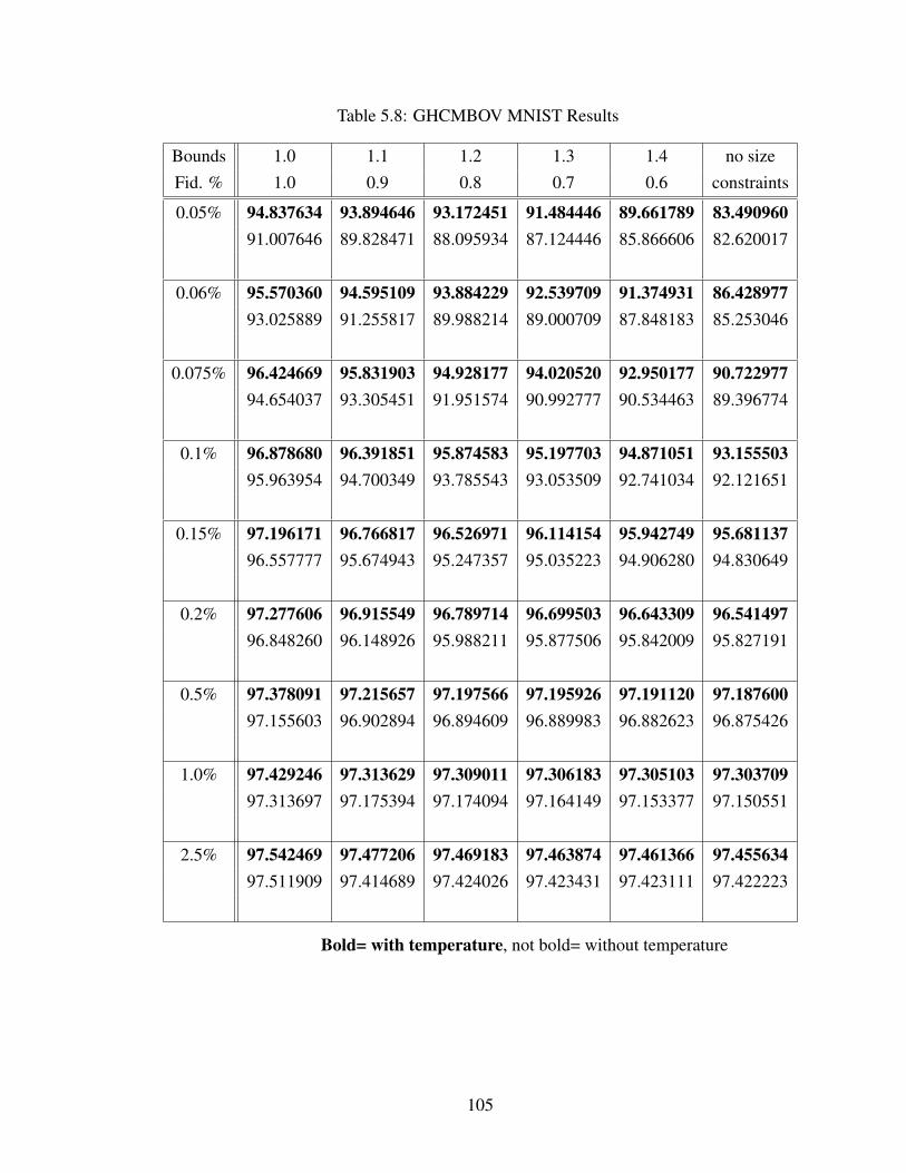
Table 5.8: GHCMBOV MNIST Results
Bounds 1.0 1.1 1.2 1.3 1.4 no sizeFid. % 1.0 0.9 0.8 0.7 0.6 constraints
0.05% 94.837634 93.894646 93.172451 91.484446 89.661789 83.49096091.007646 89.828471 88.095934 87.124446 85.866606 82.620017
0.06% 95.570360 94.595109 93.884229 92.539709 91.374931 86.42897793.025889 91.255817 89.988214 89.000709 87.848183 85.253046
0.075% 96.424669 95.831903 94.928177 94.020520 92.950177 90.72297794.654037 93.305451 91.951574 90.992777 90.534463 89.396774
0.1% 96.878680 96.391851 95.874583 95.197703 94.871051 93.15550395.963954 94.700349 93.785543 93.053509 92.741034 92.121651
0.15% 97.196171 96.766817 96.526971 96.114154 95.942749 95.68113796.557777 95.674943 95.247357 95.035223 94.906280 94.830649
0.2% 97.277606 96.915549 96.789714 96.699503 96.643309 96.54149796.848260 96.148926 95.988211 95.877506 95.842009 95.827191
0.5% 97.378091 97.215657 97.197566 97.195926 97.191120 97.18760097.155603 96.902894 96.894609 96.889983 96.882623 96.875426
1.0% 97.429246 97.313629 97.309011 97.306183 97.305103 97.30370997.313697 97.175394 97.174094 97.164149 97.153377 97.150551
2.5% 97.542469 97.477206 97.469183 97.463874 97.461366 97.45563497.511909 97.414689 97.424026 97.423431 97.423111 97.422223
Bold= with temperature, not bold= without temperature
105

Table 5.9: GHCMBOV Optdigits Results.
Bounds 1.0 1.1 1.2 1.3 1.4 no sizeFid. % 1.0 0.9 0.8 0.7 0.6 constraints
0.4% 93.043167 92.380721 91.702500 91.060649 89.963372 85.29311486.865648 86.798397 86.163779 85.574292 85.096671 83.384948
0.45% 94.894706 94.226059 93.578479 92.870979 91.911868 87.92475189.758893 89.362007 88.618025 87.980644 87.639002 85.933278
0.5% 95.964875 95.175979 94.664021 93.842616 93.055881 89.75822191.762050 91.055883 90.390260 89.870701 89.310379 87.980418
0.75% 98.065649 97.192660 96.617260 96.329875 95.854929 94.68337295.895059 95.071735 94.344114 93.894988 93.623212 93.003228
1% 98.385374 97.567776 97.140872 96.914635 96.751352 96.33149597.105692 96.239815 95.692146 95.401053 95.256740 95.037457
2% 98.669635 98.011646 97.859217 97.841753 97.831984 97.80352398.132231 97.447865 97.302979 97.276091 97.267961 97.250568
3% 98.740845 98.238238 98.216459 98.186557 98.178694 98.17379098.424246 97.925253 97.865655 97.856125 97.851680 97.846831
Bold= with temperature, not bold= without temperature
5.5 Conclusions
We have presented three MBO schemes, GHCMBO, GHCMBOS, and GHCMBOV forsolving the SSL problem on a weighted graph. Our schemes are based on the graph heatcontent energy (GHC) and the theory developed in [27] and the previous chapters. Wesolve the SSL problem by minimizing an energy that combines GHC with a linear fidelityterm based on graph geodesics, inspired by the region force in [79]. GHC depends on thechoice of affinity matrix A, which induces a diffusion process on the graph. If A is PSDthen GHCMBO and GHCMBOV decrease the energy at every step, while GHCMBOS
106

decreases the energy for an even more general class of diffusion matrices. Our approachconsiderably generalizes and simplifies previous SSL graph MBO schemes [33], [60]. Theguarantee of energy dissipation and convergence to local minima is a new and importanttheoretical advance for SSL graph MBO schemes.
Experimental results on benchmark datasets show that our algorithms produce resultswith comparable or superior accuracy to other state-of-the-art methods [33], [60], [79].GHCMBOV in particular, remains accurate and effective for fidelity percentages that areout of reach for other SSL methods. In addition, all of our schemes are faster than thecurrent state of the art. GHCMBO and GHCMBOS, were nearly two orders of magnitudefaster than [33], [60], and [79] on every dataset. Our algorithms are so fast because we arefree to choose diffusions generated by extremely sparse matrices, and take very large stepsizes through the configuration space.
107

CHAPTER 6
Conclusion
In this work we have derived and analyzed new algorithms and convolution kernels forsimulating weighted curvature motion and solving minimal partition problems. The heartof our approach is the variational interpretation of the MBO scheme developed in [27]based on the heat content energy.
In Chapter 2, we derived new “single growth” versions of the MBO scheme that al-lowed us to guarantee unconditional stability for an extremely wide class of kernels. Inparticular, Algorithm 2.3 guarantees unconditional stability of the multi-phase scheme foressentially any network of kernels. This full level of generality is a first for threshold dy-namics schemes. We also proved some convergence results. In the two-phase case, oursingle growth scheme is shown to converge to the viscosity solution of the curvature flow.While we cannot show convergence to the flow in the multi-phase case, we show that theheat content energy Gamma-converges to the correct limiting energy under certain kernelconditions. Our Gamma-convergence result gives us hope that the energy type convergencearguments of [54] can be extended to more general MBO schemes studied here. Indeed, theadmissible kernels for our Gamma-convergence argument are the most general to date andinclude sign-changing kernels. Unfortunately, the allowed sign-changing kernels cannotinduce non-zonoidal anisotropies. We hope to address this shortcoming in future research(although progress seems difficult).
In Chapter 3, we gave a decisive and constructive answer to the inverse problem ofdesigning a kernel to induce a particular surface tension and mobility under threshold dy-namics. In two dimensions, we give a completely explicit construction of a non-negativekernel to induce any target smooth and convex pair (σ, µ) of anisotropy and mobility. Inthree dimensions, not every pair can be induced by a positive kernel. We give a completedescription of the necessary and sufficient conditions on the targets (σ, µ) for nonnegativ-ity of the kernel, and an explicit construction (modulo inversion of a Radon transform) foradmissible (σ, µ). In both cases, our kernel is smooth and compactly supported. In addi-tion, for any target smooth, convex pair (σ, µ) in any dimension, we provide a completely
108

explicit Fourier domain kernel construction. The resulting kernel is Schwartz class andnon-negative in the Fourier domain. The sum of this chapter fully answers an importantand longstanding question in the threshold dynamics community.
In Chapter 4, we introduced auction dynamics, a volume preserving variant of the MBOscheme. Auction dynamics simulates multi-phase volume preserving or volume boundedcurvature flow. Each step of the algorithm involves solving the assignment problem, whichwe efficiently approach using auction algorithms. The main benefit of our scheme is thesimultaneous update of the configuration and the Lagrange multipliers corresponding to thevolume constraints. This allows us to use the algorithm in situations where the interfacialboundaries may be extremely rough or irregular. We also show how to incorporate randomfluctuations due to temperature in the spirit of Monte-Carlo algorithms.
In Chapter 5, we extend the previous MBO algorithms to the graphical setting usingthe graph heat content energy (GHC). GHC is closely related to the graph cut, thus theminimization of GHC allows us to solve SSL graph partitioning problems. Our resultingschemes minimize GHC at every step, guaranteeing unconditional stability and conver-gence to a fixed point. Crucially, our algorithms are compatible with nearly any graphdiffusion process. This generality allows us to choose diffusions generated by extremelysparse matrices. As a result, our algorithm has a low computational complexity. Theability to work with sparse matrices and guarantee energy dissipation is a first for graphMBO schemes. Experimental results on benchmark machine learning datasets show thatour methods are comparable or superior to other state-of-the-art variational methods whilerunning faster. In particular, our basic algorithms, GHCMBO and GHCMBOS, are at leasttwo orders of magnitude faster than other state-of-the-art variational SSL methods. Ourvolume preserving method, GHCMBOV, remains effective at low fidelity percentages thatare out of reach for competing state-of-the-art variational SSL methods.
109

BIBLIOGRAPHY
[1] G. Alberti and G. Bellettini. A non-local anisotropic model for phase transitions:asymptotic behavior of rescaled energies. European J. Appl. Math., 9:261–284, 1998.
[2] F. Almgren, J. E. Taylor, and L.-H. Wang. Curvature-driven flows: a variationalapproach. SIAM Journal on Control and Optimization, 31(2):387–438, 1993.
[3] L. Ambrosio and A. Braides. Functionals defined on partitions in sets of finiteperimeter II: semicontinuity, relaxation, and homogenization. J. Math. Pures et Appl.,69:307–333., 1990.
[4] G. Barles and C. Georgelin. A simple proof of convergence for an approximationscheme for computing motions by mean curvature. SIAM J. Numer. Anal., 32:484–500, 1995.
[5] G. Barles and P. Souganidis. Convergence of approximation schemes for fully non-linear second order equations. Asymptotic Analysis, 4:271–283, 1991.
[6] J. W. Barrett, H. Garcke, and R. Nurnberg. Parametric approximation of surfaceclusters driven by isotropic and anisotropic surface energies. Interfaces and FreeBoundaries, 12:187–234, 2010.
[7] G. Bellettini and M. Paolini. Anisotropic motion by mean curvature in the context ofFinsler geometry. Hokkaido Mathematical Journal, 25:537–566, 1996.
[8] Andrea L. Bertozzi and Arjuna Flenner. Diffuse interface models on graphs for classi-fication of high dimensional data. Multiscale Modeling and Simulation, 10(3):1090–1118, 2012.
[9] Dimitri Bertsekas. A distributed algorithm for the assignment problem. Technicalreport, MIT, May 1979.
[10] Dimitri Bertsekas. Linear network optimization. MIT Press, 1991.
[11] Dimitri Bertsekas. Network Optimization: Continuous and Discrete Models. AthenaScientific, 1998.
[12] Dimitri Bertsekas and David Castanon. The auction algorithm for the transportationproblem. Annals of Operations Research, 20:67–69, 1989.
110

[13] Dimitri Bertsekas, David Castanon, and Haralampos Tsaknakis. Reverse auction andthe solution of asymmetric assignment problems. SIAM J. on Optimization, 3:268–299, 1993.
[14] E. D. Bolker. A class of convex bodies. Transactions of the American MathematicalSociety, 145:323–345, 1969.
[15] E. Bonnetier, E. Bretin, and A. Chambolle. Consistency result for a non-monotonescheme for anisotropic mean curvature flow. Interfaces and Free Boundaries,14(1):1–35, 2012.
[16] X. Bresson, T. Chan, X. Tai, and A. Szlam. Multiclass transductive learning based onL1 relaxations of cheeger cut and Mumford-Shah-Potts model. Journal of Mathemat-ical Imaging and Vision, 49(1):191–201, August 2013.
[17] L. Bronsard and B. Wetton. A numerical method for tracking curve networks movingwith curvature motion. Journal of Computational Physics, 120(1):66–87, 1995.
[18] H. Busemann and C. M. Petty. Problems on convex bodies. Mathematica Scandinav-ica, 4:88–94, 1956.
[19] J. Cheeger. A lower bound for the smallest eigenvalue of the Laplacian. In Problemsin Analysis, pages 195–199. 1970.
[20] Y.-G. Chen, Y. Giga, and S. Goto. Uniqueness and existence of viscosity solutionsof generalized mean curvature flow equations. Journal of Differential Geometry,33:749–786, 1991.
[21] R. R. Coifman, S. Lafon, A. B. Lee, M. Maggioni, B. Nadler, F. Warner, and S. W.Zucker. Geometric diffusions as a tool for harmonic analysis and structure definitionof data: Diffusion maps. PNAS, 2005.
[22] E. De Giorgi. New problems on minimizing movements. In C. Baiocchi and J. L.Lions, editors, Boundary value problems for PDE and applications, pages 81–98.Masson, 1993.
[23] A. di Carlo, M. E. Gurtin, and P. Podio-Guidugli. A regularized equationfor anisotropic motion-by-curvature. SIAM Journal on Applied Mathematics,52(4):1111–1119, 1992.
[24] E. Dijkstra. A note on two problems in connexion with graphs. Numerische Mathe-matik, 1:269–271, 1959.
[25] M. Elsey and S. Esedoglu. Threshold dynamics for anisotropic surface energies. AMSMathematics of Computation, 2017.
[26] S. Esedoglu and M. Jacobs. Convolution kernels and stability of threshold dynamicsmethods. Technical report, University of Michigan, August 2016. Under review.
111

[27] S. Esedoglu and F. Otto. Threshold dynamics for networks with arbitrary surfacetensions. Communications on Pure and Applied Mathematics, 68(5):808–864, 2015.
[28] S. Esedoglu and Y.-H. Tsai. Threshold dynamics for the piecewise constant Mumford-Shah functional. Journal of Computational Physics, 211(1):367–384, 2006.
[29] Selim Esedoglu, Matt Jacobs, and Pengo Zhang. Kernels with prescribed surfacetension and mobility for threshold dynamics schemes. Journal of ComputationalPhysics, 337:62–83, 15 May 2017.
[30] L. C. Evans. Convergence of an algorithm for mean curvature motion. Indiana Uni-versity Mathematics Journal, 42:553–557, 1993.
[31] L. C. Evans and J. Spruck. Motion of level sets by mean curvature. I. Journal ofDifferential Geometry, 33:635–681, 1991.
[32] P. Funk. Uber flachen mit lauter geschlossenen geodatischen linien. Math. Ann.,74(2):278–300 (German), 1913.
[33] C. Garcia-Cardona, E. Merkurjev, A. L. Bertozzi, A. Flenner, and A. G. Percus. Multi-class data segmentation using diffuse interface methods on graphs. IEEE Transactionson Pattern Analysis and Machine Intelligence, 36(8):1600–1613, 2014.
[34] R. J. Gardner. Intersection bodeis and the Busemann-Petty problem. Transactions ofthe American Mathematical Society, 342(1):435–445, 1994.
[35] R. J. Gardner. A positive answer to the Busemann-Petty problem in three dimensions.Annals of Mathematics, 140:435–447, 1994.
[36] A.V. Goldberg. Solving minimum-cost flow problems by successive approximation.In STOC 87, November 1986.
[37] A.V. Goldberg. Efficient graph algorithms for sequential and parallel computer. Tech-nical report, Laboratory for Computer Science, M.I.T., 1987.
[38] A.V. Goldberg and R.E. Tarjan. Solving minimum cost flow problems by successiveapproximation. In Proc. 19th ACM STOC, May 1987.
[39] Paul Goodey and Wolfgang Weil. Centrally symmetric convex bodies and the spheri-cal Radon transform. Journal of Differential Geometry, 35:675–688, 1992.
[40] Matt Grayson. Shortening embedded curves. The Annals of Mathematics, 129(1):71–111, 1989.
[41] Thomas Hales. The honeycomb conjecture. Discrete and Computational Geometry,25(1):1–22, 2001.
[42] M. Hein and S. Setzer. Beyond spectral clustering - tight relaxations of balancedgraph cuts. In Advances in Neural Information Processing Systems 24 (NIPS 2011),2011.
112

[43] S. Helgason. The Radon Transform, volume 5 of Progress in Mathematics.Birkhauser, Boston, MA, 1999.
[44] C. Herring. The Physics of Powder Metallurgy, chapter Surface tension as a motiva-tion for sintering, pages 143–179. McGraw Hill, 1951.
[45] Tony Hoare. Algorithm 65: Find. Communications of the ACM, 4(7):321–322, 1961.
[46] E. A. Holm, G. N. Hassold, and M. A. Miodownik. Dimensional effects on anisotropicgrain growth. In G. Gottstein and D. Molodov, editors, Recrystallization and GrainGrowth, pages 239–244, RWTH Aachen, Germany, August 2001. First Joint Interna-tional Conference on Recrystallization and Grain Growth, Springer-Verlag.
[47] T. Y. Hou, J. S. Lowengrub, and M. J. Shelley. Removing the stiffness from interfacialflows with surface tension. Journal of Computational Physics, 114(2):312–338, 1994.
[48] H. Ishii, G. E. Pires, and P. E. Souganidis. Threshold dynamics type approxima-tion schemes for propagating fronts. Journal of the Mathematical Society of Japan,51:267–308, 1999.
[49] Matt Jacobs. A fast MBO scheme for multiclass data segmentation. In Scale Spaceand Variational Methods in Computer Vision, 2017.
[50] Matt Jacobs, Ekaterina Merkurjev, and Selim Esedoglu. Auction dynamics: A volumepreserving MBO scheme. Technical report, In preperation, 2017.
[51] C Kaynak. Methods of combining multiple classifiers and their applications to hand-written digit recognition. Master’s thesis, Institute of Graduate Studies in Science andEngineering, Bogazici University, 1995.
[52] D. Kinderlehrer, I. Livshitz, and S. Taasan. A variational approach to modeling andsimulation of grain growth. SIAM Journal on Scientific Computing, 28(5):1694–1715,2006.
[53] Harold Kuhn. The hungarian method for the assignment problem. Naval ResearchLogistics Quarterly, 2, 1955.
[54] T. Laux and F. Otto. Convergence of the thresholding scheme for multi-phase mean-curvature flow. Technical report, Max Planck Institute for Mathematics in the Sci-ences, 2015.
[55] S. Luckhaus and T. Sturzenhecker. Implicit time discretization for the mean curvatureflow equation. Calculus of Variations and Partial Differential Equations, 3(2):253–271, 1995.
[56] E. Lutwak. Intersection bodies and dual mixed volumes. Advances in Mathematics,71:232–261, 1988.
[57] J. Malik and J. Shi. Normalized cuts and image segmentation. IEEE Transactions onPattern Analysis and Machine Intelligence, 22(8):888–905, August 2000.
113

[58] P. Mascarenhas. Diffusion generated motion by mean curvature. CAM Report 92-33,UCLA, July 1992. (URL = http://www.math.ucla.edu/applied/cam/index.html).
[59] Peter McMullen and Egon Schulte. Abstract Regular Polytopes. Macmillan, 2002.
[60] E. Merkurjev, A. Bertozzi, and F. Chung. A semi-supervised heat kernel pagerankMBO algorithm for data classification. Submitted, 2016.
[61] Ekaterina Merkurjev, Justin Sunu, and Andrea L. Bertozzi. Graph MBO method formulticlass segmentation of hyperspectral stand-off detection video. In IEEE Interna-tional Conference on Image Processing, October 2014.
[62] B. Merriman, J. K. Bence, and S. Osher. Motion of multiple junctions: a level setapproach. Journal of Computational Physics, 112(2):334–363, 1994.
[63] B. Merriman, J. K. Bence, and S. J. Osher. Diffusion generated motion by meancurvature. In J. Taylor, editor, Proceedings of the Computational Crystal GrowersWorkshop, pages 73–83. AMS, 1992.
[64] M. Miranda, D. Pallara, F. Paronetto, and M. Preunkert. Short-time heat flow andfunctions of bounded variation in RN . Ann. Fac. Sci. Toulouse, Mathematiques,16(1):125–145, 2007.
[65] F. Morgan. Lowersemicontinuity of energy clusters. Proceedings of the Royal Societyof Edinburgh, 127A:819–822, 1997.
[66] W. W. Mullins. Two dimensional motion of idealized grain boundaries. J. Appl. Phys.,27:900–904, 1956.
[67] D. Mumford and J. Shah. Optimal approximations by piecewise smooth functions andassociated variational problems. Communications on Pure and Applied Mathematics,42:577–685, 1989.
[68] James Munkres. Algorithms for the assignment and transportation problems. Journalof the Society for Industrial and Applied Mathematics, 5(1), 1957.
[69] S.A. Nene, S.K. Nayar, and H. Murase. Columbia object image library (coil-100).Technical report, Columbia University, 1996.
[70] Alexander Zien Olivier Chapelle, Bernhard Scholkopf. Semi-Supervised Learning.The MIT Press, 2006.
[71] S. Osher and J. Sethian. Fronts propagating with curvature-dependent speed: Algo-rithms based on Hamilton-Jacobi formulation. Journal of Computational Physics,79:12–49, 1988.
[72] S. J. Ruuth. Efficient algorithms for diffusion-generated motion by mean curvature.PhD thesis, The University of British Columbia, 1996.
114

[73] S. J. Ruuth. A diffusion generated approach to multiphase motion. Journal of Com-putational Physics, 145:166–192, 1998.
[74] S. J. Ruuth. Efficient algorithms for diffusion-generated motion by mean curvature.Journal of Computational Physics, 144:603–625, 1998.
[75] S. J. Ruuth and B. Merriman. Convolution generated motion and generalized Huy-gens’ principles for interface motion. SIAM Journal on Applied Mathematics, 60:868–890, 2000.
[76] S. J. Ruuth and B. Wetton. A simple scheme for volume-preserving motion by meancurvature. Journal of Scientific Computing, 19(1):373–384, 2003.
[77] D. Weaire and R. Phelan. A counter-example to kelvin’s conjecture on minimal sur-faces. Philosophical Magazine Letters, 69:107–110, 1994.
[78] X. Xu, D. Wang, and X. Wang. An efficient threshold dynamics method for wettingon rough surfaces. arXiv:1602.04688, February 2016.
[79] K. Yin, Xue-Cheng Tai, and S. J. Osher. An effective region force for some variationalmodels for learning and clustering. Technical report, UCLA, 2016.
[80] S. X. Yu and J. Shi. Multiclass spectral clustering. In Ninth IEEE InternationalCoference on Computer Vision, 2003, volume 1, pages 313–319, October 2003.
[81] Lihi Zelnik-Manor and Pietro Perona. Self-tuning spectral clustering. Advances inneural information processing systems, 2004.
115