The European Journal of FinanceVol. 13, No. 8, 717–739, December 2007

Algorithmic Trading Patterns in Xetra Orders

JOHANNES PRIX, OTTO LOISTL, & MICHAEL HUETLInvestment Banking and Catallactics Group, Vienna University of Economics and Business Administration,Vienna, Austria

ABSTRACT Computerized trading controlled by algorithms – “Algorithmic Trading” – has become afashionable term in investment banking. We investigate a set of Xetra order data to find traces of algorithmictrading by studying the lifetimes of cancelled orders. Even though it is widely agreed that an algorithmmust randomize its order activities to avoid exploitation by other traders, we still find systematic patternsin the submission and cancellation of certain Xetra orders, indicating the activity of algorithmic trading.The trading patterns observed might be interpreted as fishing for profitable roundtrips.

KEY WORDS: Market microstructure, algorithmic trading, cancellations, order lifetime, Xetra

1. Introduction

Algorithmic trading has become a standard technique in most investment firms. Algorithms arecapable of submitting ever larger streams of orders to the electronic order book at increasingspeeds.A recent statement by Deutsche BörseAG mentioned that 37% of trades currently originatefrom algorithmic trading (cf. Deutsche Börse AG (2006)), while Gomber and Groth (2006, p. 50)estimate up to 40% of algorithmic trade volume. It seems quite obvious that an algorithm should“randomize how it sends orders in the market, how it prices orders, and the way it cancels andreplaces those orders. Otherwise, someone could see that order coming and prepare to make moneyon it” (quote from Hiresh Mittal of ITG in Mehta (2005), cited in: Schwartz et al. (2006, p. 301)).

In response to the needs of algorithmic trading, continuing improvements in the network infra-structure of Deutsche Börse AG have caused roundtrip1 times to decline to ever lower levels.Recent roundtrip times have fallen to the level of 20 milliseconds and are expected to reach alevel of 10 milliseconds by April 2007 (cf. Deutsche Börse AG (2007)). At the same time, leadingevent stream processing systems have to cope with the challenge of reaching latencies in therange of milliseconds (cf. Stonebraker et al. (2006), Bates and Palmer (2006), Aleri Labs (2006)).Event stream processing tracks, as the term indicates, individual events (see Luckham (2002)).Investigating algorithmic trading therefore also benefits from investigating individual events, e.g.,the insertion, cancellation or completion of single orders.

Correspondence Address: Johannes Prix, Investment banking and Catallactics Group,Vienna University of Economics andBusiness Administration, Althanstrasse 39–45, 1090 Vienna, Austria. Fax: +43-1-31336-761; Tel.: +43-1-31336-4168;Email: johannes.prix@wu-wien.ac.at

1351-847X Print/1466-4364 Online/07/080717–23 © 2007 Taylor & FrancisDOI: 10.1080/13518470701705538

718 J. Prix et al.

Short roundtrip times in combination with the low decision-making latency of algorithms offerideal trading conditions for fully automated trading systems, enabling them to respond to newconditions in the sub-second range. As these response times are key to the analysis of algorithmictrades, we note the high precision of the time stamps in our dataset. These time stamps of orderevents are recorded with a precision of one hundredth of a second. Thus, using this set of individualorders, we are able to carry out detailed lifetime studies and search for algorithms using lifetimedeviations in the sub-second range.

In this paper, we primarily focus on the time dimension for identifying traces of algorithmictrades. With respect to time analysis there is a large body of literature on so-called financialduration processes that allow us to define basically any event of interest and the correspondingduration sequence; the applications so far mostly focus on aggregates and not on individualorders. Graming and Maurer (2000) adapt the autoregressive conditional duration (ACD) modelproposed by Engle and Russell (1998) to analyse (NYSE) price durations. Engle and Dufour(2000) investigate NYSE price durations by applying a vector autoregressive model, originallyproposed by Hasbrouck (1991). Engle and Lunde (2003) generalize the ACD model to analyseboth transactions and quotes in a Trade and Quote (TAQ) database from the NYSE. Hall andHautsch (2006) model the most aggressive order submissions using an autoregressive conditionalintensity model, which was originally introduced by Russel (1999). In these models, the financialdurations are commonly generated by data “thinning”, i.e., the selection of particular points in theall-embracing trading (point) process (see, e.g., Bauwens and Giot (2001, p. 45)). Trade durationis defined as the time between two transactions and price duration is defined as the equivalent ofa first passage time of the price process (see, for instance, Hautsch (2004, p. 4)). The analysis ofdurations is restricted if quotes and trades are in different databases such as in the NYSE’s TAQdatabase.Another issue is in identifying the buyer and seller initiated trades (see Engle and Dufour(2000) who used Trade, Order, Report, Quote (TORQ) data). Lee and Ready (1991) proposedthe “five seconds rule” and the “mid-quote rule”, respectively, for approximately solving theseissues. For a treatment of problems in the data preparation process for the application of durationmodels, see Hautsch (2004).

In our study, we calculate and analyse the lifetime of an order by tracking the points of thetrading process (events) within an order. In our dataset from the Xetra system of Deutsche BörseAG, orders are identified by a unique identifier. Therefore, for each order, the full history of eventssuch as order insertion, deletion, execution, partial execution or modification can be followed. Foreach event the full details of the order, except identification of the trader or the exchange memberinvolved, are given. The detailedness of the dataset allows the identification of each order involvedin a matching of orders as well as the identification of buyer and seller initiated trades. We arenot forced to rely on the approximation rules mentioned above for TAQ/TORQ like databases.

For investigating the algorithmic trading features in the Xetra order book, we concentrate ouranalysis on the lifetimes of the so-called no-fill-deletion orders, i.e., orders that are inserted andsubsequently cancelled. We find previously undiscovered specific patterns in cancelled orders’lifetimes from the reconstructed order book data of Deutsche Börse’s Xetra system. We investi-gate these patterns in cancelled orders’ lifetimes on an order-by-order basis, i.e., by analysing theexisting orders and the corresponding detailed order event entries in the order book. Our inves-tigation leads us to evidence of activities of automatons placing orders on the buy and sell side.We define the criteria for filtering sequences of orders, which we term constant-initial-cushion(CIC) orders, providing a case study of algorithmic trading in the Xetra Order book. The strategybehind these algorithmic orders seems to be consistent with a result from Handa and Schwartz(1996). In that paper, the authors investigated the use of limit orders versus market orders but also

Algorithmic Trading Patterns in Xetra Orders 719

tested a pure limit orders trategy that consisted of a network of bid and ask orders placed aroundthe current price.

Several other studies investigating order lifetimes and cancellations have been conducted.A study focusing on the lifetimes of limit orders executed was carried out by Lo et al. (2002). Theauthors use survival analysis and a data sample of orders from an institutional investor to developan econometric model of limit-order execution lifetimes. They report detailed survival functionsfor time-to-completion, time-to-first-fill for the range from 0 to 60 minutes. Hasbrouck and Saar(2005) investigate Island ECN orders and mention a large proportion of “fleeting orders”, i.e.,very short-lived orders with lifetimes below two seconds terminated by cancellation inside thespread. They attribute them to the search for “hidden liquidity” made possible by the microstruc-ture of the Island ECN. Boehmer et al. (2005) analyse the special open limit order book andfind decreasing order sizes and faster cancellation, and thus shorter lifetime of cancelled ordersthan before the introduction of the NYSE Open Book service. This NYSE Open Book serviceprovides information about limit orders every 10 seconds and, as the authors note, may be tooslow for certain types of automated trading strategies that investors may want to implement offthe exchange floor.

The remainder of the paper is organized as follows: Section 2 describes the market model ofDeutsche Börse’s Xetra system as well as the specifics of our dataset. Section 3 examines thelifetimes of cancelled Xetra orders, illustrates patterns resulting from algorithmic trading activityand gives a possible explanation for the strategy of the algorithmic trades. Section 4 summa-rizes and concludes. In keeping with an increasingly common practice, only the main results arepresented in the paper. More detailed results are available on request from the correspondingauthor.

2. The Frankfurt Stock Exchange and the Dataset

2.1 The Database

As the basis for our research, we use the complete record of the order book events from the Xetrasystem of Deutsche Börse AG. Two different time periods, each of which contains six tradingdays were used. The first database contains the record of all order book changes occuring in thetime from 8 to 15 December 2004. The second data base contains all changes in the time from 5to 12 January 2005.

The first database consists of 4 794 741 entries and the second one of 5 014 200 entries recordschanges in the electronic order book of the Xetra system. Note that the database entries themselvesdo not explicitly contain information such as best bid and best ask or current reference price.Instead, a database entry is generated whenever an order is entered into the system, partiallyexecuted, fully executed, cancelled, modified, automatically entered or automatically cancelled.Every such order event is time-stamped at the moment it is processed by the Xetra order booksoftware. The time-stamps in our dataset feature a precision of One hundredth of a second whilethe Xetra system itself operates with a precision level of One thousandth of a second. Thus, thetiming accuracy in our dataset almost matches the accuracy of the real Xetra engine. The matchingalgorithm of Xetra relies on these time-stamps to execute trades according to the price-time priorityrules given in the Xetra market model (cf. Deutsche Börse AG (2004)).

Information such as best bid, best ask and current reference price can be reconstructed fromthe order events. In order to find the best bid, best ask or current order book depth for any giventime t , it is necessary to find the subset of orders valid at time t , according to the Xetra market

720 J. Prix et al.

model and the order restrictions given as parameters to each order. These orders are then sortedin a table according to price priority such that the current available volume for buying and sellingat any given limit can be computed. A similar procedure can be used to find the current referenceprice. By sorting order events according to their time stamps and then finding the most recentorder execution price before t , the reference price can be reconstructed from the order data. Theindividual events will be described in more detail in Section 2.4.

In order to avoid data-snooping effects, the initial research for this paper, including definitionof the filtering criteria for CIC orders, was done using the database containing all order bookevents from 8 to 15 December 2004. The tables and figures in this paper were then generated outof sample using the second database that describes all changes to the order book occurring in thesix trading days from 5 to 12 January 2005.

2.2 The Frankfurt Stock Exchange

Deutsche Börse AG runs the Frankfurt Stock Exchange (FWB). It is by far the most importantamong the eight German stock exchanges and offers floor trading as well as fully-electronictrading on Xetra. Approximately 97% of all trading involving the DAX-30 stocks of our sampleare done via Xetra (cf. Deutsche Börse AG (2005)). While many of the DAX-30 stocks are alsolisted on other exchanges, the vast majority of trading for these stocks happens on the Xetrasystem.

Xetra offers remote access: some 350 brokers and broker firms from 18 countries participatein the trading. Xetra trading is organized as a hybrid system combining auctions and contin-uous trading. For the DAX-30 stocks in our sample, a pre-trading phase from 7:30 to 8:50hours offers the opportunity to enter orders into Xetra. The functioning of order driven mar-kets is thoroughly explained by Schwartz et al., (2006, pp. 73–75). Following the pre-tradephase, an opening auction with a randomly timed end around 9:00 hours provides the first exe-cutions of each trading day (cf. Deutsche Börse AG (2003)). After the opening auction, thesystem switches to continuous trading until the intraday auction at 13:00 hours, again with arandomly timed ending. This intraday auction is again followed by continuous trading until theclosing auction at 17:30 hours, again featuring a randomly timed ending. A volatility break andan additional auction occur whenever the price leaves a pre-fixed price band.2 Continuous tradingfollows the price-time priority rule (cf. Deutsche Börse AG (2004) for the details of the matchingalgorithm).

2.3 Order Types

The Xetra system allows four different types of orders:

Limit order. Limit Orders comprise the lion’s share of the Xetra order book. The Limit Order ischaracterized by a limit on the price that the submitter is willing to accept. Those orders witha lower (higher) price limit for an ask (bid) order get higher priority for being executed.

Market order. Market Orders do not feature any restriction on the price the submitter is willing toaccept. Therefore, they are executed immediately, possibly generating several trades, sometimeseven with different transaction prices if the order size is larger than the best order on the otherside. This property is commonly known as “walking up the book”.

Market-to-limit order. Market-to-Limit orders are similar to market orders matching the best orderon the other side, if completely filled. If the Market-to-Limit order is not completely filled at

Algorithmic Trading Patterns in Xetra Orders 721

the best limit on the other side, the remaining part will enter the order book as a limit orderwith exactly that limit.

Iceberg orders. Iceberg orders split up the entire volume into visible parts of smaller size and onlydisplay one such part at a time as a limit order. As soon as the disclosed limit order is completelyfilled, a new limit order of the same size will be entered into the order book automatically bythe system. This process is repeated until the whole volume of the iceberg order is matched orthe order is cancelled.

For limit and market orders, additional flags and restrictions governing the execution handlingcan be supplied. The most important restrictions are the following three flags:

Fill-or-kill (F). This restriction will cause the system to check if the order can be completelymatched immediately. If this is possible, the order will be executed. Otherwise it will be deletedimmediately.

Immediate-or-Cancel (I). This restriction will cause the system to execute all matches that arepossible at the order’s arrival time point.Any remaining part that cannot be matched immediatelywill be deleted immediately.

Triggered-Stop-Order (S). This order is entered into the order book automatically as soon as thepredefined stopping conditions are met.

2.4 Order Event Codes and Order Event Sequences

In the following, we use a database that contains all changes to the order book occurring on thesix trading days in the time from 5 to 12 January 2005, as described in Section 2.1. It consistsof 5 014 200 database entries recording changes in the electronic order book of the Xetra system.The database entries consist of different event types. Each event type’s code and frequency arelisted in Table 1.

Table 1. Frequency of different events in the database

Event type Event code Absolute frequency % Entryb % Terminationc

Order entrya 1 2 284 628 99.98Order modification 2 36 165Order cancellation 3 1 626 896 70.15Order filled completely 4 675 232 29.12Order partially filled 5 373 760Order deleted automatically 6 16 597 0.72Technical Entry 101 461 0.02Technical Cancellation 103 461 0.02

Frequency of different events in the database along with their event code found in the time 5–12 January 2005. A total of5 014 200 database entries were examined. Absolute count data are given in the middle column, while the two rightmostcolumns list the percentage of orders started/ended via each respective event code.aDue to the restriction of the dataset to a certain observation period, there were some orders where the order entry wasnot observable in the dataset. Similarly, there were orders without a suitable end of code 3, 4, 103 or 6. This is the reasonwhy the sum of order entries (code 1 and code 101 adds up to 2 284 628 + 461 = 2 285 089) does not match the sum oforder terminations (code 3, 4, 6 and 103 adds up to 1 626 896 + 675 232 + 16 597 + 461 = 2 319 186).bPercentage of orders, that are entered via a 1 resp. 101 code. Hundred percent comprises all order entry events in thedatabase.cPercentage of orders terminated via a 3, 4, 6 resp. 103 event. Hundred percent comprises all order terminating events inthe database.

722 J. Prix et al.

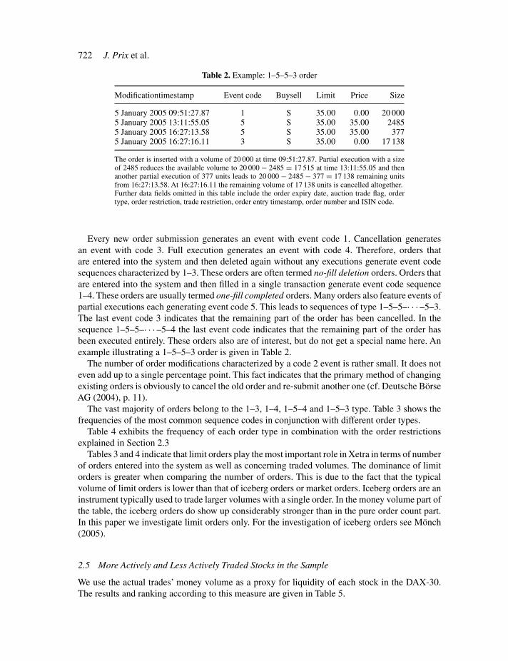
Table 2. Example: 1–5–5–3 order

Modificationtimestamp Event code Buysell Limit Price Size

5 January 2005 09:51:27.87 1 S 35.00 0.00 20 0005 January 2005 13:11:55.05 5 S 35.00 35.00 24855 January 2005 16:27:13.58 5 S 35.00 35.00 3775 January 2005 16:27:16.11 3 S 35.00 0.00 17 138

The order is inserted with a volume of 20 000 at time 09:51:27.87. Partial execution with a sizeof 2485 reduces the available volume to 20 000 − 2485 = 17 515 at time 13:11:55.05 and thenanother partial execution of 377 units leads to 20 000 − 2485 − 377 = 17 138 remaining unitsfrom 16:27:13.58. At 16:27:16.11 the remaining volume of 17 138 units is cancelled altogether.Further data fields omitted in this table include the order expiry date, auction trade flag, ordertype, order restriction, trade restriction, order entry timestamp, order number and ISIN code.

Every new order submission generates an event with event code 1. Cancellation generatesan event with code 3. Full execution generates an event with code 4. Therefore, orders thatare entered into the system and then deleted again without any executions generate event codesequences characterized by 1–3. These orders are often termed no-fill deletion orders. Orders thatare entered into the system and then filled in a single transaction generate event code sequence1–4. These orders are usually termed one-fill completed orders. Many orders also feature events ofpartial executions each generating event code 5. This leads to sequences of type 1–5–5–· · · –5–3.The last event code 3 indicates that the remaining part of the order has been cancelled. In thesequence 1–5–5–· · · –5–4 the last event code indicates that the remaining part of the order hasbeen executed entirely. These orders also are of interest, but do not get a special name here. Anexample illustrating a 1–5–5–3 order is given in Table 2.

The number of order modifications characterized by a code 2 event is rather small. It does noteven add up to a single percentage point. This fact indicates that the primary method of changingexisting orders is obviously to cancel the old order and re-submit another one (cf. Deutsche BörseAG (2004), p. 11).

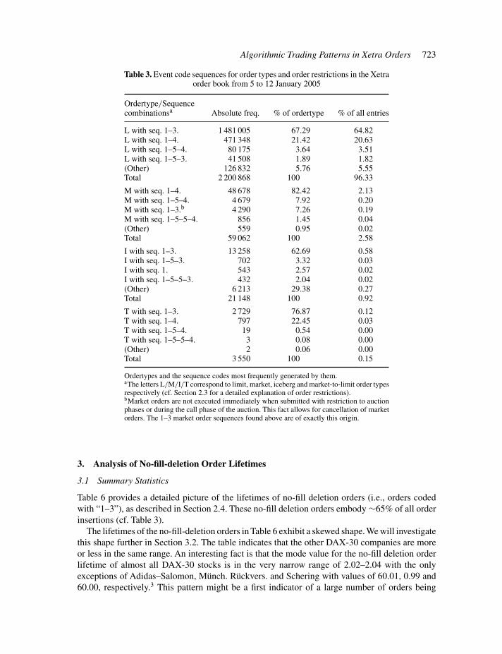
The vast majority of orders belong to the 1–3, 1–4, 1–5–4 and 1–5–3 type. Table 3 shows thefrequencies of the most common sequence codes in conjunction with different order types.

Table 4 exhibits the frequency of each order type in combination with the order restrictionsexplained in Section 2.3

Tables 3 and 4 indicate that limit orders play the most important role in Xetra in terms of numberof orders entered into the system as well as concerning traded volumes. The dominance of limitorders is greater when comparing the number of orders. This is due to the fact that the typicalvolume of limit orders is lower than that of iceberg orders or market orders. Iceberg orders are aninstrument typically used to trade larger volumes with a single order. In the money volume part ofthe table, the iceberg orders do show up considerably stronger than in the pure order count part.In this paper we investigate limit orders only. For the investigation of iceberg orders see Mönch(2005).

2.5 More Actively and Less Actively Traded Stocks in the Sample

We use the actual trades’ money volume as a proxy for liquidity of each stock in the DAX-30.The results and ranking according to this measure are given in Table 5.

Algorithmic Trading Patterns in Xetra Orders 723

Table 3. Event code sequences for order types and order restrictions in the Xetraorder book from 5 to 12 January 2005

Ordertype/Sequencecombinationsa Absolute freq. % of ordertype % of all entries

L with seq. 1–3. 1 481 005 67.29 64.82L with seq. 1–4. 471 348 21.42 20.63L with seq. 1–5–4. 80 175 3.64 3.51L with seq. 1–5–3. 41 508 1.89 1.82(Other) 126 832 5.76 5.55Total 2 200 868 100 96.33

M with seq. 1–4. 48 678 82.42 2.13M with seq. 1–5–4. 4 679 7.92 0.20M with seq. 1–3.b 4 290 7.26 0.19M with seq. 1–5–5–4. 856 1.45 0.04(Other) 559 0.95 0.02Total 59 062 100 2.58

I with seq. 1–3. 13 258 62.69 0.58I with seq. 1–5–3. 702 3.32 0.03I with seq. 1. 543 2.57 0.02I with seq. 1–5–5–3. 432 2.04 0.02(Other) 6 213 29.38 0.27Total 21 148 100 0.92

T with seq. 1–3. 2 729 76.87 0.12T with seq. 1–4. 797 22.45 0.03T with seq. 1–5–4. 19 0.54 0.00T with seq. 1–5–5–4. 3 0.08 0.00(Other) 2 0.06 0.00Total 3 550 100 0.15

Ordertypes and the sequence codes most frequently generated by them.aThe letters L/M/I/T correspond to limit, market, iceberg and market-to-limit order typesrespectively (cf. Section 2.3 for a detailed explanation of order restrictions).bMarket orders are not executed immediately when submitted with restriction to auctionphases or during the call phase of the auction. This fact allows for cancellation of marketorders. The 1–3 market order sequences found above are of exactly this origin.

3. Analysis of No-fill-deletion Order Lifetimes

3.1 Summary Statistics

Table 6 provides a detailed picture of the lifetimes of no-fill deletion orders (i.e., orders codedwith “1–3”), as described in Section 2.4. These no-fill deletion orders embody ∼65% of all orderinsertions (cf. Table 3).

The lifetimes of the no-fill-deletion orders in Table 6 exhibit a skewed shape. We will investigatethis shape further in Section 3.2. The table indicates that the other DAX-30 companies are moreor less in the same range. An interesting fact is that the mode value for the no-fill deletion orderlifetime of almost all DAX-30 stocks is in the very narrow range of 2.02–2.04 with the onlyexceptions of Adidas–Salomon, Münch. Rückvers. and Schering with values of 60.01, 0.99 and60.00, respectively.3 This pattern might be a first indicator of a large number of orders being

724J.P

rixetal.Table 4. Importance of different order types concerning number of orders and money volume traded in the time from 5 to 12 January 2005

Number of orders submittedb Money volume tradedc

Limit Market MtL Iceberg Limit Market MtL IcebergRestrictiona percentage percentage percentage percentage percentage percentage percentage percentage

None 93.96 2.40 0.16 0.93 80.08 6.32 0.13 8.24F 0.01 0.00 0.00 0.00 0.14 0.20 0.00 0.00I 2.34 0.03 0.00 0.00 0.02 0.00 0.00 0.00S 0.03 0.16 0.00 0.00 4.83 0.03 0.00 0.00

Total percentage 96.34 2.59 0.16 0.93 85.07 6.55 0.13 8.24

In abs. figures 2 200 868 59 062 3 550 21 148 34 841 574 719 2 683 281 921 53 501 579 3 375 360 805

Observation period was the time from 5 to 12 January 2005. A total of 2 284 628 orders were examined. Percentage of the money volume and number of orders belonging to eachcategory are shown above.aOrderrestriction “F” means Fill-Or-Kill, Orderrestriction “I” means Immediate-or-Cancel and “S” means Triggered-Stop-Order.bThe left part of the table shows the relative frequency of each order type entered into the Xetra system in conjunction with each order restriction. Hundred percent correspondsto all orders submitted. Thus, in the left part of the table all orders are counted, regardless of whether they are executed or cancelled. The total percentage figures do not sum upto 100% due to rounding effects.cThe right part of the table shows the relative amount of money volume traded using each order type in conjunction with each order restriction. Money volume was computedusing the size of the execution in shares times the price of the transaction per share. Thus, if the price is better than a possible limit supplied, the transaction price was used forthe computation. The cancelled part of any order is disregarded in this part of the table. Hundred percent in the right part of the table corresponds to the total money volumetraded on Xetra in the observation period. The total percentage figures do not sum up to 100% due to rounding effects.

Algorithm

icTrading

Patternsin

Xetra

Orders

725

Table 5. More actively and less actively traded stocks

Money volumea Order countsb

Stock Insertions in ¤ (partial) exec. in ¤ % of total Cancels in ¤ % of total # Insertions # (Partial) exec. # Cancels

Adidas–Salomon 1 770 215 224 447 125 622 25.26 1 286 488 383 72.67 56 950 17 964 44 821Allianz 8 790 277 310 2 420 874 661 27.54 6 365 267 254 72.41 139 377 53 282 107 569Altana 1 246 653 282 327 284 804 26.25 884 871 110 70.98 45 370 18 590 32 164BASF 5 417 235 455 1 559 059 342 28.78 3 806 098 197 70.26 101 962 41 656 73 566Bay.Hypo-Vereinsbk. 3 809 997 784 1 440 028 234 37.80 2 420 967 668 63.54 73 804 35 883 53 476Bay.Motoren Werke 3 514 440 533 1 017 405 425 28.95 2 603 134 296 74.07 85 254 31 886 68 350Bayer 4 331 672 091 1 499 615 910 34.62 2 800 234 703 64.65 88 208 44 242 59 384Commerzbank 2 983 413 630 957 340 370 32.09 2 070 980 883 69.42 71 676 32 220 54 939Continental 2 066 085 303 505 688 538 24.48 1 519 165 870 73.53 56 939 21 832 42 015Daimlerchrysler 6 127 425 933 1 887 165 222 30.80 4 258 908 966 69.51 106 081 46 882 78 365Deutsche Bank 9 469 106 165 3 427 840 346 36.20 5 997 248 669 63.33 121 055 60 878 83 319Deutsche Börse 1 416 524 808 422 635 469 29.84 945 572 830 66.75 34 948 14 174 25 332Deutsche Post 1 812 172 774 481 907 183 26.59 1 314 871 778 72.56 51 807 21 389 37 590Dt.Telekom 11 828 478 731 4 943 385 187 41.79 6 709 010 564 56.72 102 992 66 925 60 236E.ON 7 223 954 037 2 023 701 781 28.01 5 121 734 538 70.90 101 513 46 768 70 762Fresen. Med. Care 785 318 869 168 525 398 21.46 582 477 219 74.17 30 382 10 302 23 026Henkel 1 300 108 649 307 276 160 23.63 958 371 953 73.71 54 805 14 370 44 954Infineon Tech. 2 307 849 938 1 051 246 991 45.55 1 259 620 703 54.58 60 000 35 302 38 333Linde 1 239 932 379 303 736 968 24.50 893 918 504 72.09 48 285 15 698 38 181Lufthansa 1 177 439 125 397 502 755 33.76 737 285 375 62.62 42 659 19 028 30 512MAN 2 369 511 487 542 591 278 22.90 1 789 611 094 75.53 45 841 19 812 33 763

(continued)

726J.P

rixetal.

Table 5. Continued

Money volumea Order countsb

Stock Insertions in ¤ (partial) exec. in ¤ % of total Cancels in ¤ % of total # Insertions # (Partial) exec. # Cancels

Metro 3 051 119 590 961 073 566 31.50 2 033 491 197 66.65 75 733 30 020 55 788Münch. Rückvers. 6 704 429 897 1 727 628 726 25.77 5 003 312 853 74.63 126 827 40 623 102 038RWE 5 681 840 719 2 059 831 162 36.25 3 568 859 575 62.81 92 385 54 657 57 242SAP 9 736 429 511 3 590 803 808 36.88 6 133 401 159 62.99 128 310 72 740 82 167Schering 3 220 077 589 1 169 923 324 36.33 2 005 412 669 62.28 59 785 34 784 36 808Siemens 9 617 142 107 2 983 210 594 31.02 6 517 991 136 67.77 117 034 62 447 75 561Thyssenkrupp 1 803 884 997 599 383 000 33.23 1 148 294 495 63.66 49 433 25 196 33 266TUI 1 372 789 752 325 475 811 23.71 1 024 373 231 74.62 43 419 18 139 32 086Volkswagen 3 790 013 654 1 404 451 392 37.06 2 532 581 837 66.82 72 255 41 303 51 283

Total/Average 125 965 541 324 40 953 719 025 30.75 84 293 558 706 68.21 2 285 089 1 048 992 1 626 896

Ranking of the DAX-30 stocks according to money volume traded during the trading days from 5 to 12 January 2005. The top four and the bottom four stocks will be analysedin more detail in the next sections.aTotal money volume inserted, traded and cancelled are given in the left section of the table. The cancelled money volume was computed using limit value times number ofshares cancelled instead of a real price times number of shares traded.bCount of total orders inserted, orders fully or partially executed and pure cancellations without any execution (“no-fill deletions”) are given in the right section of the table. Theusual double counting of money volume applies for the trades. The sum of # (partial) executions and # cancels is greater than the # insertions due to the fact that every partialexecution is counted. Therefore, the percentage figures were omitted in the “order counts” section.

Algorithmic Trading Patterns in Xetra Orders 727

Table 6. Summary statistics of the lifetimes of all no-fill-deletion orders from 5 to 12 January 2005

Stock name Min 1st Q. Mode Median Mean 3rd Q. Max N

Dt.Telekom 0.07 5.23 2.03 24.09 679.10 106.90 627 500.00 56 038SAP 0.06 2.96 2.02 11.94 375.40 55.00 620 400.00 75 786Deutsche Bank 0.06 4.53 2.02 14.69 266.20 55.10 514 300.00 75 891Siemens 0.07 3.16 2.03 12.43 360.80 54.95 584 700.00 70 202Allianz 0.05 2.98 2.02 11.16 278.00 46.38 521 400.00 99 937RWE 0.06 4.67 2.02 22.65 471.80 80.56 532 600.00 52 059E.ON 0.08 3.50 2.02 14.86 297.50 59.95 629 100.00 64 980Daimlerchrysler 0.07 4.33 2.02 17.70 338.00 62.09 625 400.00 70 683Münch.Rückvers. 0.07 4.08 0.99 12.46 240.60 39.59 526 200.00 96 735BASF 0.07 4.52 2.02 18.29 321.30 60.10 625 600.00 69 632Bayer 0.07 4.87 2.03 24.14 474.80 88.65 519 900.00 55 017Bay.Hypo-Vereinsbk. 0.07 6.97 2.03 27.90 437.00 93.74 527 500.00 47 848Volkswagen 0.08 5.39 2.02 29.54 469.50 95.98 538 300.00 43 147Schering 0.07 7.10 60.00 38.70 407.30 109.70 529 100.00 34 242Infineon Tech. 0.08 6.84 2.03 33.06 1 098.00 135.30 622 600.00 34 370Bay.Motoren Werke 0.06 4.60 2.02 18.04 406.50 60.20 585 800.00 60 642Metro 0.06 8.65 2.03 24.09 265.10 69.38 610 500.00 52 951Commerzbank 0.06 4.76 2.02 20.80 469.50 80.47 433 700.00 48 861Thyssenkrupp 0.08 5.21 2.03 25.46 836.10 108.60 623 800.00 31 008MAN 0.07 7.59 2.02 34.72 425.80 119.10 584 000.00 31 024Continental 0.06 7.05 2.02 27.91 351.40 86.08 457 300.00 39 803Deutsche Post 0.07 5.33 2.03 27.14 474.20 110.00 434 800.00 35 130Adidas–Salomon 0.07 3.89 60.01 19.41 265.00 67.06 535 800.00 42 332Deutsche Börse 0.07 4.58 2.03 28.14 307.90 112.10 94 650.00 23 820Lufthansa 0.06 6.48 2.04 34.68 721.20 132.00 534 900.00 27 915Altana 0.07 5.82 2.02 33.49 307.60 119.10 432 700.00 30 451TUI 0.07 5.50 2.02 26.30 433.10 103.00 625 600.00 29 488Henkel 0.06 4.65 2.03 18.17 192.10 60.23 273 500.00 43 433Linde 0.07 7.45 2.03 26.54 277.00 84.96 200 200.00 35 791Fresen. Med. Care 0.07 4.59 2.03 36.81 364.80 132.70 229 800.00 22 066

DAX-30 POOL 0.05 4.58 2.02 19.50 393.50 69.38 629 100.00 1 501 282

Summary statistics of the no-fill-deletion order lifetimes for each stock as well as for the pool of all DAX-30 stockstogether are given in the middle columns. All lifetimes were measured in seconds and recorded for orders placed in thetime from 5 to 12 January 2005. Total number of observations for each stock are given in the rightmost column.

timed by software programs supporting the human trader or by fully automated trading programsusually termed algorithmic traders.

3.2 The No-fill-deletion Order Lifetime Distribution

The plot in Figure 1 investigates the distribution of the lifetime of no-fill-deletion orders. To give aprecise picture, we differentiate four different time scales. We apply the kernel density estimation4

procedure to characterize the lifetime frequency.The spikes in the plots and the overall shape of the plots in Figure 1 reveal, to our knowledge,

a previously undiscovered pattern – cancellations occur predominantly after some very “special”lifetimes. At one and two seconds, there is a local maximum. After 30, 60, 120 and 180 secondsthere are more such local maxima. Less obvious are the weaker spikes at exactly four, five and

728 J. Prix et al.

Figure 1. Kernel density estimates for the lifetime of no-fill-deletion orders: We reduced the dataset to thelifetimes contained in the intervals [0; 2.5], [0; 7.5], [0; 67.5] and [0; 197.5] for all DAX-30 stocks to givesmall scale as well as larger scale pictures of the distribution of order lifetimes. The kernel bandwidth used

and the number of orders contained in each interval is given below each of the four graphs, respectively

six seconds. The same pattern can be found for most of the individual stocks of the DAX-30.Figure 2 below illustrates the remarkable similarity in cancellation patterns for the four mostactively traded and the five least actively traded stocks given for the range of 0–67.5 seconds.

For the stock TUI, the peak at 60 seconds is not observable (see also Section 3.3.1). The patternof no-fill-deletion order lifetimes is present throughout the daily trading time. Figure 3 illustratesthe observed no-fill-deletion order lifetimes for different subsets of the trading day.

The one-fill-completed orders with a lifetime greater than zero are not terminated by cancel-lation or execution. The execution of orders is beyond their control, and therefore, not subject topeaking of lifetimes at the end of each update cycle.

3.3 Investigation of Lifetime Peaks at Multiples of 60 Seconds

3.3.1 Example of automated order placements – constant-initial-cushion orders. A closer lookat the no-fill deletion orders (i.e., orders with sequence code “1–3”) with lifetimes close to thelifetime peaks shown in Figure 1 gives the following picture. The peaks at multiples of 60 seconds

Algorithmic Trading Patterns in Xetra Orders 729

Figure 2. Kernel density estimates for the lifetime of no-fill-deletion orders in the interval [0;67.5] secondsfor the most actively traded (Dt.Telekom, SAP, Deutsche Bank, Siemens) and the five least actively traded(Altana, TUI, Henkel, Linde, Fresen.Med.Care) stocks in the time from 5 to 12 January 2005 (cf. Table 5)

can be explained (at least partly) by sequences of orders which we term constant-initial-cushion(CIC) orders.

The orders of such a sequence have the following properties. A CIC order sequence consistsof both bids and asks, i.e., of order placements on both sides of the market, where the bidsand asks have the same order size. The name “CIC orders” is motivated by the observed orderlimits. All bids (asks) of such a CIC order sequence have the same constant cushion at insertion

Figure 3. Kernel density estimates for the lifetime of no-fill-deletion orders occuring at daytime 9:00 to12:00 hours (left plot), from 12:00 to 15:00 hours (middle plot) and from 15:00 to 17:30 hours (right plot).

Each plot shows the density for lifetimes in the interval [0;67.5] for all DAX-30 stocks

730 J. Prix et al.

(constant-initial-cushion), where cushion is defined as

cushion ={

best bid limit − bid limit for a bid

ask limit − best ask limit for an ask

However, the bids’ CIC is not necessarily equal to the asks’ CIC. Further, the lifetimes of CICorders rounded to the nearest second are multiples of 60 seconds. Hence, cancellation takes placeonly at 60 seconds or multiples of 60 seconds after insertion. In all observed cases, at the timeof cancellation the order cushion is not equal to the CIC. Furthermore, for each CIC order withrounded lifetime equal to l × 60 seconds with l ≥ 2, l ∈ N, the following can be said. In allobserved cases, the observed cushions at 1 × 60, . . . , (l − 1) × 60 seconds, since insertions areequal to the CIC. The observed cushions at any other point of time during the lifetime of a CICorder are not necessarily equal to the CIC. After a CIC order is cancelled (except for the last bidand ask cancellation in a sequence), a new CIC order is inserted. If a CIC bid (ask) is cancelled,another CIC bid (ask) is inserted at a limit equal to best bid − CIC (best ask + CIC).

Table 7 and Figure 4 illustrate a part of a sequence of CIC orders observed for SAP AG on 5January 2005 between 13:51:36 and 13:56:35 hours. At 13:51:36.00 (at 13:51:35.96) hours a CICask (a CIC bid) was inserted with an order size of 1200 shares and CIC of 26 cents. At the time ofthese insertions, the best bid and best ask were 129.87 ¤ and 129.90 ¤, respectively. Sixty secondslater, at around 13:52:36 hours, the best bid was still at 129.87 ¤, while the best ask had moved upto 130.01 ¤. Therefore, the cushion of the CIC bid remained at 26 cents, while the cushion of theCIC ask decreased to 15 cents. Consequently, the CIC ask was deleted and a new CIC ask wasinserted at limit 130.01 + 0.26 = 130.27 ¤. The deleted CIC ask had a lifetime of 60.05 seconds.Approximately 60 seconds later, the cushion of both the CIC bid and ask had changed due to themoving best offers. The CIC ask at 130.27 ¤ (CIC bid at 129.61 ¤) was deleted and a new CICask at 130.06 + 0.26 = 130.32 ¤ (a new CIC bid at 129.90 − 0.26 = 129.64 ¤) was inserted. Thedeleted ask (bid) had a lifetime of 60.03 seconds (120.07 seconds). Hence, the lifetimes of theCIC orders depended on the variability of the best bid and ask (see Figure 4). The lifetimes ofthe CIC orders shown in Table 7 and Figure 4 varied around 60 and 120 seconds. As the best askshowed higher variation than the best bid in this period (see Figure 4), we observe five insertionson the ask side and only three on the bid side.

In Table 7, CIC orders are illustrated for only a small snapshot of five minutes. To identifyall CIC order sequences for a stock we define explicit filtering criteria. In order to avoid datasnooping, we used data from 8 to 15 December 2004 to get the defining criteria for CIC orders

Table 7. Sample CIC orders placed on 6 January 2005 for SAP

Time at insertion Lifetime Limit BestBid BestAsk CIC (B)id/(hh:mm:ss.cs) (Sec.) (Euro) (Euro) (Euro) (Euro) Size (A)sk

13:51:36.00 60.05 130.16 129.87 129.90 0.26 1200 A13:52:36.05 60.03 130.27 129.87 130.01 0.26 1200 A13:53:36.08 59.91 130.32 129.90 130.06 0.26 1200 A13:54:35.99 60.17 130.28 129.90 130.02 0.26 1200 A13:55:36.16 59.96 130.20 129.87 129.94 0.26 1200 A

13:51:35.96 120.07 129.61 129.87 129.90 0.26 1200 B13:53:36.03 120.12 129.64 129.90 130.06 0.26 1200 B13:55:36.15 59.95 129.61 129.87 129.94 0.26 1200 B

Algorithmic Trading Patterns in Xetra Orders 731

Figure 4. CIC orders for SAP AG on 5 January 2005 between 13:51:35 and 13:56:35 hours with lifetimesof multiples of 60 seconds (dotted lines). If the best bid (thin straight line) or best ask (thin dashed line)changes such that the inserted bid or ask (thick lines) has no longer the CIC at multiples of 60 seconds sinceinsertion, the corresponding order is deleted and a new order is inserted at the CIC. Obviously, deletion only

occurs at order lifetimes of multiples of 60 seconds since insertion

and applied them to investigating data spanning the period between 5 and 12 January 2005. Theapplied filtering criteria for identifying CIC order sequences are given as follows.

1. All orders in a CIC order sequence are no-fill-deletion orders, i.e., orders with sequencecode “1–3”.

2. A sequence of CIC orders consists of bids and asks. Whenever a bid in this sequence is validin the order book, an ask of this sequence also has to be valid in the order book and vice versa.

3. A sequence includes at least three orders (i.e., one bid and two asks, or two bids and one ask).Hence, the number of orders in a sequence N ≥ 3.

4. All bids and asks in a sequence of CIC orders fulfill the following criteria.(a) The bids’ and asks’ cushions at insertion are constant. The bids’ cushion at insertion is not

necessarily equal to the asks’ cushion at insertion.(b) The bids’ and asks’ volumes are constant. The bids’ volume is equal to the asks’ volume.(c) The lifetimes of the bids and asks rounded to the nearest second are equal to or a multiple

of 60 seconds.

The result of the application of these filtering criteria to order book data for SAP AG between5 and 12 January 2005 is given in Table 8. As shown in Table 8, we identified 14 sequences ofCIC orders, where the cushions and order sizes of CIC orders for different CIC order sequences

732 J. Prix et al.

Table 8. All CIC orders placed between 5 and 12 January 2005 for SAP

Period CIC Lifetime

Day Begin End Bid Ask Min. Median Max. Number(dd-mm-yyyy) (hh:mm:ss.cs) (hh:mm:ss.cs) (Euro) (Euro) Size (sec.) (sec.) (sec.) N

5 January 2005 10:00:34.86 14:00:35.73 0.26 0.26 1900 59.68 60.04 419.99 2985 January 2005 14:14:35.67 14:38:35.89 0.18 0.49 1200 59.84 59.99 120.06 275 January 2005 14:45:35.99 15:47:36.33 0.26 0.26 1900 59.86 60.04 299.88 915 January 2005 15:53:36.41 15:58:36.47 0.26 0.26 1000 59.90 60.02 60.08 105 January 2005 16:05:36.68 16:36:36.50 0.16 0.55 1100 59.72 60.02 239.52 245 January 2005 17:15:36.91 17:26:36.88 0.18 0.49 1300 59.86 60.06 119.90 15

6 January 2005 10:02:34.68 17:28:37.30 0.26 0.26 1200 59.70 60.06 419.84 580

7 January 2005 10:00:35.33 14:28:36.72 0.27 0.27 2200 59.72 60.03 840.23 3407 January 2005 14:51:36.95 17:28:37.64 0.26 0.26 1700 59.68 60.01 239.60 181

10 January 2005 10:01:35.52 17:27:37.91 0.28 0.27 1100 59.74 60.06 360.08 567

11 January 2005 11:36:13.38 16:00:15.14 0.26 0.26 1700 59.78 60.04 300.03 35411 January 2005 16:27:15.50 17:27:15.93 0.26 0.26 1000 59.73 60.02 120.30 61

12 January 2005 10:05:35.66 15:47:38.22 0.25 0.25 1700 59.61 60.04 480.19 42212 January 2005 16:01:38.02 17:27:38.23 0.25 0.25 1600 59.64 60.01 120.18 136

varied. Between 5 and 12 January 2005 the order size varied between 1000 and 2200 for SAP. TheCIC ranged between 16 and 27 cents for the CIC bids and between 25 and 55 cents for the CICasks for SAP. The maximum lifetime of a CIC order was 840.23 seconds. For all CIC orders wefind rounded lifetimes of 60 seconds and multiples thereof. A technical reasoning for the marginalfluctuations in CIC order lifetimes is given in Section 3.5.

A possible explanation for these observations of CIC order sequences may be that an automatedorder placement system updates CIC orders at intervals of 60 seconds by cancellation and sub-sequent insertion such that the orders’ cushions fulfills the properties described above. A furtherlook at the order book suggests that the intraday change of the order volume or cushions for theCIC orders is because of the order matching of a CIC bid or ask. At the end of each of the indicatedperiods (excluding end of day periods) shown in Table 8, we find executed orders, each with aninsertion time equal to the deletion time of the last observed CIC order in the correspondingsequence. Further, each of these executed orders has the same cushion and order size as the lastdeleted CIC order of the corresponding sequence.

However, the dataset does not allow us to identify the order submitting trader. Therefore,we cannot make a definite statement about these suggestions. In the next section, we furthersubstantiate our explanations by investigating all 30-DAX stock for the occurrences of CIC ordersequences.

3.3.2 CIC order statistics for all DAX 30 stocks. Table 9 shows footprints of CIC order insertionsfor almost all DAX-30 stocks. The cushion ratio shown in Table 9 expressing the cushion as apercentage of the median price observed between 5 and 12 January is around 0.2%. A lower boundfor the bid and ask cushion is observed at 4 cents for most of the DAX stocks. The existence ofan absolute lower bound on the cushion would explain the high cushion ratios for stocks withlow median prices such as Lufthansa and Infineon. On the basis of this observation, one canapproximate the cushion for each stock by max(0.2% · Median Price, 0.04).

Algorithm

icTrading

Patternsin

Xetra

Orders

733

Table 9. CIC orders for all DAX30 stocks observed between 5 to 12 January 2005

Bid CIC Ask CIC Lifetime Size Money Volumeb Pricec Sized

Median Ratioa Median Ratioa Min. Median Max. Abs. Rel. Median(Euro) (%) (Euro) (%) (sec.) (sec.) (sec.) Min. Median Max. (Tsd. Euro) (%) (Euro) Median

Dt. Telekom 0.04 0.24 0.04 0.24 59.56 120.05 1 860.12 8900 11 900 15 000 248 779 4.34 16.53 4500SAP 0.26 0.20 0.26 0.20 59.61 60.04 840.23 1000 1700 2200 625 098 12.09 129.78 250Deutsche Bank 0.13 0.20 0.13 0.20 59.51 60.07 780.11 1900 2900 4400 502 989 10.09 66.33 586Siemens 0.12 0.19 0.12 0.19 59.51 60.07 1 439.89 2000 3300 4800 449 210 7.93 61.95 1000Allianz 0.19 0.20 0.19 0.20 59.64 60.05 540.05 100 1600 2700 486 106 8.69 96.48 300RWE 0.09 0.21 0.09 0.21 59.51 60.10 900.17 100 5500 7200 361 828 11.79 43.05 690E.ON 0.13 0.19 0.13 0.19 59.54 60.07 960.14 2300 2900 4900 444 115 9.92 67.01 800Daimlerchrysler 0.07 0.20 0.07 0.20 59.68 60.14 1 140.18 4300 6700 8300 408 159 11.20 35.82 860Münch.Rückvers. 0.19 0.21 0.18 0.20 59.58 60.07 1 080.14 1300 1700 3000 461 495 10.35 92.27 200BASF 0.11 0.21 0.10 0.19 59.58 60.10 840.20 2300 3000 5500 419 634 12.68 52.43 500Bayer 0.05 0.21 0.05 0.21 59.50 119.78 2 160.04 5200 6700 10 000 250 767 10.71 24.05 814Bay.Hypo-Vereinsbk. 0.04 0.23 0.04 0.23 59.71 119.90 4 200.32 4700 8200 15 000 216 155 10.59 17.04 900Volkswagen 0.07 0.20 0.07 0.20 59.62 60.17 1 199.90 200 5400 8100 246 830 11.56 35.89 500Schering 0.11 0.20 0.11 0.20 59.53 60.08 1 259.96 1300 2200 3500 296 413 18.39 54.10 370Infineon Tech. 0.04 0.51 0.04 0.51 59.52 179.89 5 520.38 8000 12 200 15 000 84 426 8.35 7.86 1200Bay.Motoren Werke 0.07 0.20 0.07 0.20 59.53 60.22 1 980.17 200 5600 8200 346 582 15.47 34.30 400Metro 0.08 0.19 0.08 0.19 59.55 60.15 2 220.24 1800 3200 6000 203 185 11.55 41.30 200Commerzbank 0.04 0.25 0.04 0.25 59.66 119.99 2 700.33 6300 7400 14 400 175 417 10.03 16.09 800Thyssenkrupp – – – – – – – – – – – – 16.31 800

(continued)

734J.P

rixetal.

Table 9. Continued

Bid CIC Ask CIC Lifetime Size Money Volumeb Pricec Sized

Median Ratioa Median Ratioa Min. Median Max. Abs. Rel. Median(Euro) (%) (Euro) (%) (sec.) (sec.) (sec.) Min. Median Max. (Tsd. Euro) (%) (Euro) Median

MAN 0.06 0.20 0.06 0.20 59.62 119.88 1 560.17 1000 1400 2100 68 880 4.26 29.35 200Continental 0.10 0.21 0.10 0.21 59.51 60.18 1 079.99 1200 2100 2900 165 254 12.52 48.31 200Deutsche Post 0.04 0.24 0.04 0.24 59.58 120.10 2 520.25 400 8300 13 800 195 333 17.09 16.97 900Adidas-Salomon 0.24 0.20 0.24 0.20 59.52 60.08 1 800.02 100 400 1400 128 004 11.50 118.51 100Deutsche Börse – – – – – – – – – – – – 44.74 200Lufthansa 0.04 0.38 0.04 0.38 59.52 120.14 2 760.26 6100 8500 12 300 101 180 16.87 10.65 800Altana 0.10 0.22 0.09 0.20 59.55 119.74 1 860.28 100 1400 2700 105 566 13.43 45.13 200TUI – – – – – – – – – – – – 18.09 300Henkel 0.13 0.20 0.13 0.20 59.52 60.13 2 220.30 100 900 1300 123 841 14.66 66.44 114Linde 0.10 0.21 0.10 0.21 59.62 119.74 2 100.10 100 1200 2000 72 297 9.20 48.23 163Fresen.Med.Care 0.12 0.21 0.12 0.21 59.52 60.29 1 620.16 300 600 900 49 165 9.85 58.05 130

Stocks are ordered according to traded money volume.aThe cushion ratio is calculated as cushion divided by the median price.bThe price is calculated as the median of all prices observed between 5 and 12 January for each stock.cThe total money volume is given in absolute terms (in thousands) and as fraction of the total money volume of all no-fill-deletion orders for the stock.dSize is given as the median of the inserted order size of all no-fill-deletion orders.

Algorithmic Trading Patterns in Xetra Orders 735

For Deutsche Börse, Thyssen Krupp and TUI the rows in Table 9 are empty, because CIC ordersare not identifiable for any of the three companies. This observation is consistent with the resultreported in Figure 2, where for TUI no significant lifetime peaks for 60 seconds could be found.The lifetime distribution of Deutsche Börse AG and Thyssen Krupp, which are not plotted here,exhibit similar lifetime distributions lacking significant peaks at multiples of 60 seconds.

The volumes of the CIC orders are multiples of 100 shares. Stocks with a cushion equal to4 cents have the highest maximum volumes ranging between 12 500 and 15 000 stocks. Themaximum volume of 15 000 stocks was observed for Deutsche Telekom, Bay. Hypo Vereinsbankand Infineon. Comparing the median CIC order volume with the median order volume of allno-fill-deletion orders shows a higher average volume for CIC orders.

The maximum lifetime of CIC observed ranges between 540 and 5220 seconds. The overallmaximum lifetime of 5220 seconds was observed for Infineon for both the CIC bid and askinserted at 12:46:35 hours and cancelled at 14:18:35 hours on 5 January 2005. During this periodin which the intraday auction also took place (see Section 2.2) the best bid and ask remained thesame. The stocks with CIC order cushion equal to 4 cents all have a median lifetime at around120 seconds. Infineon has an even median lifetime of 179.89 seconds.

The column Money volume in Table 9 shows that CIC orders represent between 4.3% and 18.4%of all no-fill-deletion orders observed between 5 and 12 January 2005.

3.4 Trading Strategy Behind CIC Orders

The trading strategy behind the placement of CIC orders closely corresponds to the limit ordertrading pattern investigated in Handa and Schwartz (1996). The authors of that paper suggestedplacing a network of bid and ask limit orders with cushions of 1%, 2%, 3%, 4% and 5% andrevising the limit orders and placing a new network of limit orders upon each execution. Theytested the strategy for the DOW-30 stocks and found significant positive returns from resultingroundtrip trades. The CIC strategy differed insofar as it used a different cushion size (0.19%–0.51% cushion instead of 1% cushion in Handa and Schwartz (1996)) and periodic updates insteadof updates only upon order execution.

3.5 Distribution of CIC Orders Lifetimes

The lifetimes of CIC orders reported in the previous sections are not exactly equal to multiplesof 60 seconds, but vary within a range of approximatlely one fourth of a second. Figure 5 showsthe observed lifetimes of CIC orders plotted as histograms and fitted to normal distributions withsample means equal to 60.01 and 120.01 seconds and sample standard deviation of about 0.11and 0.12 seconds, respectively.

Both lifetime distributions deviate from the Gaussian distribution and are leptokurtic. For bothdistributions the Kolmogorov–Smirnov test rejects the normality hypothesis at the 1% significancelevel.

The peak around, e.g., 60 second lifetimes for CIC orders might lead to the conclusion thatcomputer software updates orders on the basis of a 60 seconds lifetime. However, periodicupdates inside the exchange might not explain the fluctuations around the order lifetime of 60seconds.

A factor that might cause the fluctuations around 60 seconds is the electronic network con-necting the exchange with exchange members. We assume that all signals are generated insidethe exchange member group. If we assume that the signals are transmitted through an electronic

736 J. Prix et al.

Figure 5. Lifetime distribution of observed CIC orders for all DAX stocks (except for Deutsche Börse,TUI and Thyssen Krupp) placed between 5 and 12 January 2005 (histogram). The thick line representsthe normal distribution with estimated parameters μ̂ = mean and σ̂ = stdev. Sample kurtosis (kurt) and

skewness (skew) are given

network and might have to travel longer distances, then this might explain some of the order life-times’ fluctuations – usually a real-time data feed provided by the exchange (or other companiesspecializing in providing data) transmits input to the exchange member. The exchange memberreacts and enters a new order at time T 1. The signal travels through the network and arrives at timeT 2. The time spent on the way to the exchange might be subject to possible network delays. Thetimestamp on the order is generated in the exchange and therefore already carries the delay thathas occurred from T 1 to T 2. After a fixed time interval, like 60 seconds, counting from time T 1,the exchange member updates its positions. Let us assume that it decides to cancel the order. Asignal is then emitted at time T 3. The signal again travels through the network layer and arrives attime T 4 in the exchange. Another timestamp is recorded at arrival. This timestamp again alreadycontains the delay that occurred between T 3 and T 4. If the network speed is not constant, butsubject to perturbations, then this would generate variation in the order lifetime from T 2 to T 4,even when the time between T 1 and T 3 is always 60 seconds or a multiple thereof.

It is a well-known fact among network specialists that latency distribution of network trafficusually exhibits an approximately Gaussian shape. There are papers documenting that even veryfew participants in the network are usually sufficient for the network traffic time distribution toexhibit Gaussian features (cf. Meent et al. (2006)). Deviations of the network traffic distributionfrom Gaussianity is treated, for instance, in Jin et al. (2002).

Hence, the delays might be a simple consequence of communication via the electronic networkmedia. Such a conclusion suggests that further investigations of the electronic infrastructure of amarket place and the remote market participants might be necessary, as this might be of relevancewith respect to best execution issues.

4. Summary

Our findings indicate the existence of previously undiscovered patterns in the order book’s struc-ture when investigating the second and sub-second range of no-fill-deletion lifetimes. Bearing inmind that this range is nowadays the time frame that professional traders and algorithm designershave to cope with we investigate these patterns on an order-by-order basis, i.e., by analysingrelevant orders and the corresponding detailed order event entries in the order book.

Algorithmic Trading Patterns in Xetra Orders 737

In more detail, we analyse all no-fill-deletion orders with lifetimes equal to multiples of 60seconds and detect sequences of orders, which we term CIC orders. In order to avoid data snoop-ing, we analysed the data from 8 to 15 December 2004 to get the defining criteria for CICorders and applied these criteria for filtering and investigating data spanning the period between5 and 12 January 2005. The distance at insertion of a CIC bid (ask) limit to the best bid (ask)limit is about 0.2% of the median price for most of the 30-DAX stocks. Our investigation leadsus to evidence of activities of automatons trading on the buy and sell side, seemingly fishingfor roundtrip trade opportunities in a fashion similar to that described in Handa and Schwartz(1996). Thus, our analysis of the CIC orders has shown that results from the academic literatureare implemented in modern algorithmic trading systems and now influence some of the algo-rithmic behaviour on Xetra. It also illustrates that at least a significant part of the order flowcan be explained explicitly by analysing certain groups of orders for strategies executable byalgorithms.

A further observation is that the lifetimes of CIC orders are not exactly equal to multiples of60 seconds, but vary in the range of a few hundredths of a second. This might give an indicationof the influence of variations in the speed of the electronic network connecting the exchange withexchange members. Such a conclusion suggests to further investigate the electronic infrastructureof a market place and the remote market participants, as this might be of relevance with respectto best execution issues.

Acknowledgements

We are grateful to Deutsche Börse AG for generously providing this order dataset. We thank PeterGomber and participants of the 2007 Campus for Finance – Research Conference, (Vallendar,Germany), the Scottish Economic Society Annual Conference, (Perth, UK), and the 40th EuroWorking Group on Financial Modelling meeting (Rotterdam, Netherlands) as well as participantsof the 2007 Market Microstructure Seminar hosted at Deutsche Börse AG for valuable commentsand suggestions. We are thankful to U. Schweickert from Deutsche Börse AG for their fruitfuldiscussion on Xetra system internals.

Notes1 The time span from the moment an order is generated in the electronic system of an exchange member to the time

when a confirmation signal from the exchange arrives back at the order submitter is called roundtrip time.2 In our dataset containing all order entries of all DAX-30 stocks between 8 and 15 December 2004 and between 5 and

12 January 2005, such a volatility break occurred only twice.3 For a treatment of cancellations with lifetime lesser or equal two seconds, see Hasbrouck and Saar (2005).4 Intuitively, kernel density estimates can be understood as histograms with infinitely fine classes smoothed by moving

averages. Formally, kernel density estimates are functions of the form

f (x) = 1

n

n∑i=1

K

(x − xi

h

),

where K is the kernel function. For all plots in this paper, Gaussian kernels were used, i.e., all kernel density plots usethe formula

f (x) = 1

n

n∑i=1

K

(x − xi

h

), where K(u) = 1√

2πexp

(− 1

2u2

).

For an extensive comparison of the properties of different kernels see Hwang et al. (1994).

738 J. Prix et al.

References

Aleri Labs (2006) Powering Trading Applications with Event Stream Processing (Chicago: Aleri Inc.).Bates, J. and Palmer, M. (2006) Ten algorithmic trading trends in the lead-up to 2010. Financial Intelligence Guides,

11, 6–7.Bauwens, L. and Giot, P. (2001) Econometric Modelling of Stock Market Intraday Activity (Boston: Kluwer Acadamic

Publishers).Boehmer, E., Saar, G. and Yu, L. (2005) Lifting the veil: An analysis of pre-trade transparency at the nyse, The Journal

of Finance, 60(2), 783–815.Deutsche Börse, A. G. (2003) Xetra: Auction Plan for Stocks, Company Issued Warrants and xtf. Available at

http://deutsche-boerse.com/dbag/dispatch/en/binary/gdb_content_pool/imported_files/public_files/10_downloads/31_trading_member/10_Products_and_Functionalities/20_Stocks/40_Xetra_Auction_Plan/Xetra_Auction_Plan_e.pdf (accessed 3 November 2003).

Deutsche Börse, A. G. (2004) Xetra Market Model Equities, Release 7.1. Available at http://deutsche-boerse.com/dbag/dispatch/en/binary/gdb_content_pool/imported_files/public_files/10_downloads/31_trading_member/10_Products_and_Functionalities/20_Stocks/50_ Xetra_Market_Model/Marktmodell_Aktien_R7.pdf

Deutsche Börse,A. G. (2005) Fact Book 2005.Available at http://deutsche-boerse.com/dbag/dispatch/de/notescontent/gdb_navigation/info_center/20_Statistics/10_Spot_ Market/INTEGRATE/statistic?notesDoc=Factbook+Kassamarkt

Deutsche Börse, A. G. (2006) Deutsche Börse Quadruples Network Bandwidth for Xetra – Bandwidth Increased to 512Kbit/S – Xetra and Irish Stock Exchange Clients Benefit from Reduced Latency. Available at http://deutsche-boerse.com / dbag / dispatch / en / listcontent/gdb_navigation/technology/60_News/Content_Files/ts_sp_news_bandbreite_131206.htm (accessed 13 December 2006).

Deutsche Börse A. G. (2007) Deutsche Börse Substantially Increases Xetra Trading Speed: Comprehensive Improve-ments are Aimed at Algorithmic Trading. Available at http://deutsche-boerse.com/dbag/dispatch/en/listcontent/gdb_navigation / press / 10 _ Latest _ Press _ Releases / Content _ Files / 13_press / February_2007 / pm_news_210207.htm(accessed 21 February 2007).

Engle, R. and Dufour, A. (2000) Time and the price impact of a trade. The Journal of Finance, 55(6), 2467–2498.Engle, R. and Lunde, A. (2003) Trades and quotes: A bivariate point process. Journal of Financial Econometrics, 1(2),

159–188.Engle, R. and Russell, J. (1998) Autoregressive conditional duration: A new model for irregularly spaced transaction data.

Econometrica, 66(5), 1127–1162.Gomber, P. and Groth, S. (2006) Algorithmic trading: trends and impact on the exchange industry, in: L. Gallai, (Ed.),

Focus Newsletter of the World Federation of Exchanges, pp. 48–52. World Federation of Exchanges, Available athttp://www.world-exchanges.org/publications/Focus1206.pdf.

Grammig, J. and Maurer, K. (2000) Non-monontonic hazard functions and the autoregressive conditional duration model.The Econometrics Journal, 3(1), 16–38.

Hall, A. and Hautsch, N. (2006) Order aggressiveness and order book dynamics. Empirical Economics, 30(4), 973–1005.Handa, P. and Schwartz, R. (1996) Limit order trading. Journal of Finance, 51(5), 1835–1861.Hasbrouck, J. (1991) Measuring the information content of stock trades. The Journal of Finance, 46(1), 179–207.Hasbrouck, J. and Saar, G. (2005) Technology and Liquidity Provision: The Blurring of Traditional Definitions. Working

Paper, New York University. Available at http://pages.stern.nyu.edu/˜jhasbrou/Research/Working%20Papers/HS6.pdf

Hautsch, N. (2004) Modelling Irregularly Spaced Financial Data (Berlin: Springer).Hwang, J., Lay, S. and Lippman, A. (1994) Nonparametric multivariate density estimation: A comparative study. IEEE

Transactions on Signal Processing, 42(10), 2795–2810.Jin, Z., Shu, Y. and Yang, O. (2002) The impact of non-gaussian distribution traffic on network performance. Journal of

Computer Science and Technology, 17(1), 106–111.Lee, C. and Ready, M. (1991) Inferring trade direction from intraday data. Journal of Finance, 46(2), 733–46.Lo,A., MacKinlay, C. and Zhang, J. (2002) Econometric models of limit-order executions. Journal of Financial Economics,

65(1), 31–71.Luckham, D. (2002) The Power of Events: An Introduction to Complex Event Processing in Distributed Enterprise Systems

(Amsterdam: Addison-Wesley Longman).Meent, R., Mandjes, M. and Pras,A. (2006) Gaussian Traffic Everywhere?, in: Proceedings of the 2006 IEEE International

Conference on Communications, 10–14 June, Istanbul, Turkey.Mönch, B. (2005) Strategic Trading in Illiquid Markets (Berlin: Springer).

Algorithmic Trading Patterns in Xetra Orders 739

Russel, R. (1999) Econometric Modeling Of Multivariate Irregularly-spaced High-frequency Data. Discussion paper,University of Chicago.

Schwartz, R., Francioni, R. and Weber, B. (2006) The Equity Trader Course (Hoboken: John Wiley and Sons).Stonebraker, M., Çetintemel, U. and Zdonik, S. (2006) The eight rules of real-time stream processing, in: H. Skeete,

(Ed.), Handbook of World Stock, Derivative and Commodity Exchanges (London: Mondo Visione), Available athttp://www.exchange-handbook.co.uk/index.cfm?section=articles&action=detail&id=60623